WONDER: Weighted One-shot Distributed Ridge Regression in

Journal of Machine Learning Research 21 (2020) 1-52 Submitted 4/19; Revised 3/20; Published 4/20

WONDER: Weighted One-shot Distributed RidgeRegression in High Dimensions

Edgar Dobriban [email protected] Statistics DepartmentUniversity of PennsylvaniaPhiladelphia, PA 19104, USA

Yue Sheng [email protected]

Graduate Group in Applied Mathematics and Computational Science

University of Pennsylvania

Philadelphia, PA 19104, USA

Editor: John Shawe-Taylor

Abstract

In many areas, practitioners need to analyze large data sets that challenge conventionalsingle-machine computing. To scale up data analysis, distributed and parallel computingapproaches are increasingly needed. Here we study a fundamental and highly importantproblem in this area: How to do ridge regression in a distributed computing environment?Ridge regression is an extremely popular method for supervised learning, and has severaloptimality properties, thus it is important to study. We study one-shot methods thatconstruct weighted combinations of ridge regression estimators computed on each machine.By analyzing the mean squared error in a high-dimensional random-effects model whereeach predictor has a small effect, we discover several new phenomena.

Infinite-worker limit: The distributed estimator works well for very large numbersof machines, a phenomenon we call “infinite-worker limit”.

Optimal weights: The optimal weights for combining local estimators sum to morethan unity, due to the downward bias of ridge. Thus, all averaging methods are suboptimal.

We also propose a new Weighted ONe-shot DistributEd Ridge regression algorithm(WONDER). We test WONDER in simulation studies and using the Million Song Datasetas an example. There it can save at least 100x in computation time, while nearly preservingtest accuracy.

Keywords: distributed learning, ridge regression, high-dimensional statistics, randommatrix theory

1. Introduction

Computers have changed all aspects of our world. Importantly, computing has made dataanalysis more convenient than ever before. However, computers also pose limitations andchallenges for data science. For instance, hardware architecture is based on a model ofa universal computer—a Turing machine—but in fact has physical limitations of storage,memory, processing speed, and communication bandwidth over a network. As large datasets become more and more common in all areas of human activity, we need to thinkcarefully about working with these limitations.

c©2020 Edgar Dobriban and Yue Sheng.

License: CC-BY 4.0, see https://creativecommons.org/licenses/by/4.0/. Attribution requirements are providedat http://jmlr.org/papers/v21/19-277.html.

https://creativecommons.org/licenses/by/4.0/

http://jmlr.org/papers/v21/19-277.html

Dobriban and Sheng

How can we design methods for data analysis (statistics and machine learning) thatscale to large data sets? A general approach is distributed and parallel computing. Roughlyspeaking, the data is divided up among computing units, which perform most of the com-putation locally, and synchronize by passing relatively short messages. While the idea issimple, a good implementation can be hard and nontrivial. Moreover, different problemshave different inherent needs in terms of local computation and global communication re-sources. For instance, in statistical problems with high levels of noise, simple one-shotschemes like averaging estimators computed on local data sets can sometimes work well.

In this paper, we study a fundamental problem in this area. We are interested in linearregression, which is arguably one of the most important problems in statistics and machinelearning. A popular method for this model is ridge regression (aka Tikhonov regulariza-tion), which regularizes the estimates using a quadratic penalty to improve estimation andprediction accuracy. We aim to understand how to do ridge regression in a distributedcomputing environment. We are also interested in the important high-dimensional setting,where the number of features can be very large. In fact our approach allows the dimensionand sample size to have any ratio. We also work in a random-effects model where eachpredictor has a small effect on the outcome, which is the model for which ridge regressionis best suited.

We consider the simplest and most fundamental method, which performs ridge regressionlocally on each data set housed on the individual machines or other computing units, sendsthe estimates to a global datacenter (or parameter server), and then constructs a final one-shot estimator by taking a linear combination of the local estimates. As mentioned, suchmethods are sometimes near-optimal, and it is therefore well-justified to study them. Wewill later give several additional justifications for our work.

However, in contrast to existing work, we introduce a completely new mathematicalapproach to the problem, which has never been used for studying distributed ridge regres-sion before. Specifically, we leverage and further develop sophisticated recent techniquesfrom random matrix theory and free probability theory in our analysis. This enables usto make important contributions, that were simply unattainable using more “traditional”mathematical approaches.

To give a sense of our results, we provide a brief discussion here. We have a data setconsisting of n datapoints, for instance 1000 heart disease patients. Each datapoint hasan outcome yj , such as blood pressure, and features xj , such as age, height, electronichealth records, lab results, and genetic variables. Our goal is to predict the outcome ofinterest (i.e., blood pressure) for new patients based on their features, and to estimate therelationship of the outcome to the features.

The samples are distributed across several sites, for instance patients from differentcountries are housed in different data centers. We will refer to the sites as “machines”,though they may actually be other computing entities, such as entire computer networksor data centers. In many important settings, it can be impossible to share the data acrossthe different sites, for instance due to logistical or privacy reasons.

Therefore, we assume that each site has a subset of the samples. Our approach is totrain ridge regression on this local data. As usual, we can arrange the local data set (sayon the i-th machine) into a feature matrix Xi, where each row contains a sample (i.e.,datapoint), and an outcome vector Yi where each entry is an outcome. We compute the

2

WONDER: Weighted One-shot Distributed Ridge Regression in High Dimensions

local ridge regression estimates

βi = (X>i Xi + λiIp)−1X>i Yi,

where λi are some regularization parameters. We then aggregate them by a weightedcombination, constructing the final one-shot distributed ridge estimator (where k is thenumber of sites)

βdist =k∑i=1

wiβi.

The important questions here are:

1. How does this work?

2. How to tune the parameters? (such as the regularization parameters and weights)

Question 1 is of interest because we wish to know when one-shot methods are a goodapproach, and when they are not. For this we need to understand the performance as afunction of the key problem parameters, such as the signal strength, sample size, and dimen-sion. For question 2, the challenge is posed by the constraints of the distributed computingenvironment, where standard methods for parameter tuning such as cross-validation maybe expensive.

In this work we are able to make several crucial contributions to these questions. Wework in an asymptotic setting where n, p grow to infinity at the same rate, which effectivelygives good results for any n, p. We study a linear-random effects model, where each regressorhas a small random effect on the outcome. This is a good model for the applicationswhere ridge regression is used, because ridge does not assume sparsity, and has optimalityproperties in certain dense random effects models. Importantly, this analysis does notassume any sparsity in a high-dimensional setting. Sparsity has been one of the biggestdriving forces in statistics and machine learning in the last 20 years. Our work is in adifferent line of work, and shows that meaningful results are available without sparsity.

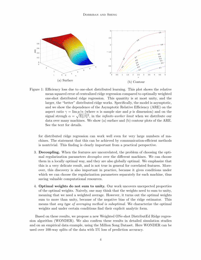
We find the limiting mean squared error of the one-shot distributed ridge estimator. Thisenables us to characterize the optimal weights and tuning parameters, as well as the relativeefficiency compared to centralized ridge regression, meaning the ratio of the risk of usualridge to the distributed estimator. This can precisely pinpoint the computation-accuracytradeoff achieved via one-shot distributed estimation. See Figure 1 for an illustration.

As a consequence of our detailed and precise risk analysis, we make several qualitativediscoveries that we find quite striking:

1. Efficiency depends strongly on signal strength. The statistical efficiency ofthe one-shot distributed ridge estimator depends strongly on signal strength. Theefficiency is generally high (meaning distributed ridge regression works well) when thesignal strength is low.

2. Infinite-worker limit. The one-shot distributed estimator does not lose all efficiencycompared to the ridge estimator even in the limit of infinitely many machines. Some-what surprisingly, this suggests that simple one-shot weighted combination methods

3

Dobriban and Sheng

03

0.2

0.4

5

AR

E

2

0.6

4

0.8

31 2

10 0

(a) Surface

0.1

0.2

0.2

0.3

0.3

0.4

0.4

0.5

0.5

0.6

0.6

0.7

0.7

0.8

0.8

0.8

0.9

0.9

0.9

0 0.5 1 1.5 2 2.5 3 3.5 4 4.5 50

0.5

1

1.5

2

2.5

3

(b) Contour

Figure 1: Efficiency loss due to one-shot distributed learning. This plot shows the relativemean squared error of centralized ridge regression compared to optimally weightedone-shot distributed ridge regression. This quantity is at most unity, and thelarger, the “better” distributed ridge works. Specifically, the model is asymptotic,and we show the dependence of the Asymptotic Relative Efficiency (ARE) on theaspect ratio γ = lim p/n (where n is sample size and p is dimension) and on thesignal strengh α =

√E‖β‖2, in the infinite-worker limit when we distribute our

data over many machines. We show (a) surface and (b) contour plots of the ARE.See the text for details.

for distributed ridge regression can work well even for very large numbers of ma-chines. The statement that this can be achieved by communication-efficient methodsis nontrivial. This finding is clearly important from a practical perspective.

3. Decoupling. When the features are uncorrelated, the problem of choosing the opti-mal regularization parameters decouples over the different machines. We can choosethem in a locally optimal way, and they are also globally optimal. We emphasize thatthis is a very delicate result, and is not true in general for correlated features. More-over, this discovery is also important in practice, because it gives conditions underwhich we can choose the regularization parameters separately for each machine, thussaving valuable computational resources.

4. Optimal weights do not sum to unity. Our work uncovers unexpected propertiesof the optimal weights. Naively, one may think that the weights need to sum to unity,meaning that we need a weighted average. However, it turns out the optimal weightssum to more than unity, because of the negative bias of the ridge estimator. Thismeans that any type of averaging method is suboptimal. We characterize the optimalweights and under certain conditions find their explicit analytic form.

Based on these results, we propose a new Weighted ONe-shot DistributEd Ridge regres-sion algorithm (WONDER). We also confirm these results in detailed simulation studiesand on an empirical data example, using the Million Song Dataset. Here WONDER can beused over 100-way splits of the data with 5% loss of prediction accuracy.

4


We also emphasize that some aspects of our work can help practitioners directly (e.g.,our new algorithm), while others are developed for deepening our understanding of thenature of the problem. We discuss the practical implications of our work in Section 4.5.

The paper is structured as follows. We discuss some related work in Section 1.1. Westart with finite sample results in Section 2. We provide asymptotic results for featureswith an arbitrary covariance structure in Section 3. We consider the special case of anidentity covariance in Section 4. In Section 5 we provide an explicit algorithm for optimallyweighted one-shot distributed ridge. We also study in detail the properties of the estimationerror, relative efficiency (including minimax properties in Section 4.6), tuning parameters(and decoupling), as well as optimal weights, including answers to the questions above.We provide numerical simulations throughout the paper, and additional ones in Section 6,along with an example using an empirical data set. The code for our paper is available atgithub.com/dobriban/dist_ridge.

1.1. Related work

Here we discuss some related work. Historically, distributed and parallel computation hasfirst been studied in computer science and optimization (see e.g., Bertsekas and Tsitsiklis,1989; Lynch, 1996; Blelloch and Maggs, 2010; Boyd et al., 2011; Rauber and Runger, 2013;Koutris et al., 2018). However, the problems studied there are quite different from the onesthat we are interested in. Those works often focus on problems where correct answers arerequired within numerical precision, e.g., 16 bits of accuracy. However, when we have noisydata sets, such as in statistics and machine learning, numerical precision is neither needednor usually possible. We may only hope for 3-4 bits of accuracy, and thus the problems aredifferent.

The area of distributed statistics and machine learning has attracted increasing attentiononly relatively recently, see for instance Mcdonald et al. (2009); Zhang et al. (2012, 2013c);Li et al. (2013); Zhang et al. (2013b,a); Chen and Xie (2014); Mackey et al. (2011); Zhanget al. (2015); Braverman et al. (2016); Jordan et al. (2019); Rosenblatt and Nadler (2016);Smith et al. (2018); Banerjee et al. (2019); Zhao et al. (2016); Xu et al. (2018); Fan et al.(2019); Lin et al. (2017); Lee et al. (2017); Volgushev et al. (2019); Shang and Cheng (2017);Battey et al. (2018); Zhu and Lafferty (2018); Chen et al. (2019, 2018); Wang et al. (2019);Shi et al. (2018); Duan et al. (2018); Liu et al. (2018); Cai and Wei (2020), and the referencestherein. See Huo and Cao (2018) for a review. We can only discuss the most closely relatedpapers due to space limitations.

Zhang et al. (2013c) study the MSE of averaged estimation in empirical risk minimiza-tion. Later Zhang et al. (2015) study divide and conquer kernel ridge regression, showingthat the partition-based estimator achieves the statistical minimax rate over all estimators,when the number of machines is not too large. These results are very general, howeverthey are not as explicit or precise as our results. In addition they consider fixed dimen-sions, whereas we study increasing dimensions under random effects models. Lin et al.(2017) improve the above results, removing certain eigenvalue assumptions on the kernel,and sharpening the rate.

Guo et al. (2017) study regularization kernel networks, and propose a debiasing schemethat can improve the behavior of distributed estimators. This work is also in the same

5

github.com/dobriban/dist_ridge

Dobriban and Sheng

framework as those above (general kernel, fixed dimension). Xu et al. (2018) propose adistributed General Cross-Validation method to choose the regularization parameter.

Rosenblatt and Nadler (2016) consider averaging in distributed learning in fixed andhigh-dimensional M-estimation, without studying regularization. Lee et al. (2017) studysparse linear regression, showing that averaging debiased lasso estimators can achieve theoptimal estimation rate if the number of machines is not too large. A related work is Batteyet al. (2018), which also includes hypothesis testing under more general sparse models.These last two works are on a different problem (sparse regression), whereas we study ridgeregression in random-effects models.

2. Finite Sample Results

We start our study of distributed ridge regression by a finite sample analysis of estimationerror in linear models. Consider the standard linear model

Y = Xβ + ε. (1)

Here Y ∈ Rn is the n-dimensional continuous outcome vector of n independent samples(e.g., the blood pressure level of n patients, or the amount of time spent on an activityby n internet users), X is the n × p design matrix containing the values of p featuresfor each sample (e.g., demographical and genetic variables of each patient). Moreover,β = (β1, . . . , βp)

> ∈ Rp is the p-dimensional vector of unknown regression coefficients.

Our goals are to predict the outcome variable for future samples, and also to esti-mate the regression coefficients. The outcome vector is affected by the random noiseε = (ε1, . . . , εn)> ∈ Rn. We assume that the coordinates of ε are independent randomvariables with mean zero and variance σ2.

The ridge regression (or Tikhonov regularization) estimator is one of the most popularmethods for estimation and prediction in linear models. Recall that the ridge estimator ofβ is

β(λ) = (X>X + nλIp)−1X>Y,

where λ is a tuning parameter. This estimator has many justifications. It shrinks the coeffi-cients of the usual ordinary least squares estimator, which can lead to improved estimationand prediction. When the entries of β and ε are i.i.d. Gaussian, and for suitable λ, it is theposterior mean of β given the outcomes, and hence is a Bayes optimal estimator for anyquadratic loss function, including estimation and prediction error.

Suppose now that we are in a distributed computation setting. The samples are dis-tributed across k different sites or machines. For instance, the data of users from a partic-ular country may be stored in a separate datacenter. This may happen due to memory orstorage limitations of individual data storage facilities, or may be required by data usageagreements. As mentioned, for simplicity we call the sites “machines”.

We can write the partitioned data as

X =

X1...Xk

, Y =

Y1...Yk

.6


Thus the i-th machine contains ni samples whose features are stored in the ni × p matrixXi and also the corresponding ni × 1 outcome vector Yi.

Since the ridge regression estimator is a widely used gold standard method, we wouldlike to understand how we can approximate it in a distributed setting. Specifically, we willfocus on one-shot weighting methods, where we perform ridge regression locally on eachsubset of the data, and then aggregate the regression coefficients by a weighted sum. Thereare several reasons to consider weighting methods:

1. This is a practical method with minimal communication cost. When communicationis expensive, it is imperative to develop methods that minimize communication cost.In this case, one-shot weighting methods are attractive, and so it is important tounderstand how they work. In a well-known course on scalable machine learning,Alex Smola calls such methods “idiot-proof” (Smola, 2012), meaning that they arestraightforward to implement (unlike some of the more sophisticated methods).

2. Averaging (which is a special case of one-shot weighting) has already been studiedin several works on distributed ridge regression (e.g., Zhang et al. (2015); Lin et al.(2017)), and much more broadly in distributed learning, see the related work sectionfor details. Such methods are known to be rate-optimal under certain conditions.

3. However, in our setting, we are able to discover several new phenomena about one-shotweighting. For instance, we can quantify in a much more nuanced way the accuracyloss compared to centralized ridge regression.

4. Weighting may serve as a useful initialization to iterative methods. In practical dis-tributed learning problems, iterative optimization algorithms such as distributed gra-dient descent or ADMM (Boyd et al., 2011) may be used. However, there are exampleswhere the first step of the iterative method has worse performance than a simple av-eraging (Pourshafeie et al., 2018). Therefore, we can imagine hybrid or warm startmethods that use weighting as an initialization. This also suggests that studyingone-shot weighting is important.

Therefore, we define local ridge estimators for each data set Xi, Yi, with regularizationparameter λi as

βi(λi) = (X>i Xi + niλiIp)−1X>i Yi.

We consider combining the local ridge estimators at a central server via a one-step weightedsummation. We will find the optimally weighted one-shot distributed estimator

βdist(w) =

k∑i=1

wiβi.

Note that, unlike ordinary least squares (OLS), the local ridge estimators are always well-defined, i.e. ni can be smaller than p. Also, for the distributed OLS estimator averaginglocal OLS solutions, it is natural to require

∑iwi = 1, because this ensures unbiasedness

(Dobriban and Sheng, 2018). However, the ridge estimators are biased, so it is not clear ifwe should put any constraints on the weights. In fact we will find that the optimal weights

7

Dobriban and Sheng

typically do not sum to unity. These features distinguish our work from prior art, and leadto some surprising consequences.

Throughout the paper, we will frequently use the notations Σ = n−1X>X and Σi =n−1i X>i Xi. A stepping stone to our analysis is the following key result.

Theorem 1 (Finite sample risk and optimal weights) Consider the distributed ridgeregression problem described above. Suppose we have a data set with n datapoints (samples),each with an outcome and p features. The data set is distributed across k sites. Each sitehas a subset Xi, Yi of the data, with the ni × p matrix Xi of features of ni samples, andthe corresponding outcomes Yi. We compute the local ridge regression estimator βi(λi) =(X>i Xi + niλiIp)

−1X>i Yi with fixed regularization parameters λi > 0 on each data set. Wesend the local estimates to a central location, and combine them via a weighted sum, i.e.,βdist(w) =

∑ki=1wiβi.

Under the linear regression model (1), the optimal weights that minimize the meansquared error of the distributed estimator are

w∗ = (A+R)−1v,

where the quantities v,A,R are defined below.

1. v is a k-dimensional vector with i-th coordinate β>Qiβ, where Qi = (Σi + λiIp)−1Σi

are p× p matrices.

2. A is a k × k matrix with (i, j)-th entry β>QiQjβ.

3. R is a k × k diagonal matrix with i-th diagonal entry n−1i σ2 tr[(Σi + λiIp)

−2Σi].

The mean squared error of the optimally weighted distributed ridge regression estimatorβdist with k sites equals

MSE∗dist(k) = E‖βdist(w∗)− β‖2 = ‖β‖2 − v>(A+R)−1v,

See Appendix F.1 for the proof. The argument proceeds via a direct calculation, recog-nizing that finding the optimal weights for combining the local estimators βi can be viewedas a k-parameter regression problem of β on βi, for i = 1, . . . , k.

This result quantifies the mean squared error of the optimally weighted distributed ridgeestimator for fixed regularization parameters λi. Later we will study how to choose theregularization parameters optimally. The result also gives an exact formula for the optimalweights. However, the optimal weights depend on the unknown regression coefficients β,and are thus not directly usable in practice. Instead, our approach is to make strongerassumptions on β under which we can develop estimators for the weights.

Computational efficiency. We take a short detour here to discuss computational effi-ciency. Here by computational efficiency we mean the total time consumption. Computingone ridge regression estimator (X>X + λIp)

−1X>Y for a fixed regularization parameter λand n×p design matrix X can be done in time O(npmin(n, p)) by first computing the SVDof X. This automatically gives the ridge estimator for all values of λ.

How much time can we save by distributing the data? Suppose first that n ≥ p, inwhich case the total time consumption is O(np2). Computing ridge locally on the i-th

8


machine takes O(nipmin(ni, p)) time. Suppose next that we distribute equally to k ofmachines, and we also have ni = n/k ≥ p. Then the time consumption is reduced toO((n/k)p2) = O(np2/k). In this case we can say that the total time consumption decreasesproportionally to the number of machines. This shows the benefit of parallel data processing.

On the other extreme, if n ≤ p, then ni = n/k ≤ p, the total time consumption is reducedfrom O(n2p) to O((n/k)2p) = O(n2p/k2). This shows that the total time consumptiondecreases quadratically in the number of machines (albeit of course the constant is muchworse). If we are in an intermediate case where n ≥ p and ni = n/k ≤ p, then the timedecreases at a rate between linear and quadratic.

2.1. Addressing reader concerns

At this stage, our readers may have several concerns about our approach. We address someconcerns in turn below.

1. Does it make sense to average ridge estimators, which can be biased?

A possible concern is that we are working with biased estimators. Would it make senseto debias them first, before weighting? A similar approach has been used for sparseregression, with the debiased Lasso estimators (Lee et al., 2017; Battey et al., 2018).However, our results allow the regularization parameters to be arbitrarily close to zero,which leads to least squares estimators, with an inverse or pseudoinverse (X>i Xi)

†.These are the “natural” debiasing estimators for ridge regression. For OLS, theseare exactly unbiased, while for pseudoinverse, they are approximately so. Hence ourapproach allows nearly unbiased estimators, and we automatically discover when thisis the optimal method.

2. Is it possible to improve the weighted sum of local ridge estimators βi in trivial ways?

One-shot weighting is merely a heuristic. If it were possible to improve it in a simpleway, then it would make sense to study those methods instead of weighting. However,we are not aware of such methods. For instance, one possibility is to try and addthe constant vector into the regression on the global parameter server, because thismay help reduce the bias. In simulation studies, we have observed that this approachdoes not usually lead to a perceptible decrease in MSE. Specifically we have foundthat under the simulation setting common throughout the paper, the MSEs with andwithout a constant term are close (see Appendix A for details).

3. Asymptotics under Linear Random-effects Models

The finite sample results obtained so far can be hard to interpret, and do not allow us to di-rectly understand the performance of the optimal one-shot distributed estimator. Therefore,we will consider an asymptotic setting that leads to more insightful results.

Recall that our basic linear model is Y = Xβ+ε, where the error ε is random. Next, wealso assume that a random-effects model holds. We assume β is random—independently ofε—with coordinates that are themselves independent random variables with mean zero andvariance p−1σ2α2. Thus, each feature contributes a small random amount to the outcome.Ridge regression is designed to work well in such a setting, and has several optimality

9

Dobriban and Sheng

properties in variants of this model. The parameters are now θ = (σ2, α2): the noiselevel σ2 and the signal-to-noise ratio α2 respectively. This parametrization is standard andwidely used (e.g. Searle et al. (2009); Dicker and Erdogdu (2017); Dobriban and Wager(2018)).

To get more insight into the performance of ridge regression in a distributed environment,we will take an asymptotic approach. Notice from Theorem 1 that the mean squared errordepends on the data only through simple functionals of the sample covariance matrices Σand Σi, such as

β>(Σi + λiIp)−1Σiβ, β>(Σi + λiIp)

−1Σi(Σj + λjIp)−1Σjβ, tr[(Σi + λiIp)

−2Σi].

When the coordinates of β are i.i.d., the means of the quadratic functionals become pro-portional to the traces of functions of the sample covariance matrices. This motivates usto adopt models from asymptotic random matrix theory, where the asymptotics of suchquantities are a central topic.

We begin by introducing some key concepts from random matrix theory (RMT) whichwill be used in our analysis. We will focus on ”Marchenko-Pastur” (MP) type samplecovariance matrices, which are fundamental and popular in statistics (see e.g., Bai andSilverstein (2010); Anderson (2003); Paul and Aue (2014); Yao et al. (2015)). A key conceptis the spectral distribution, which for a p×p symmetric matrix A is the distribution FA thatplaces equal mass on all eigenvalues λi(A) of Σ. This has cumulative distribution function(CDF) FA(x) = p−1

∑pi=1 1(λi(A) ≤ x). A central result in the area is the Marchenko-

Pastur theorem, which states that eigenvalue distributions of sample covariance matricesconverge (Marchenko and Pastur, 1967; Bai and Silverstein, 2010). We state the requiredassumptions below:

Assumption 1 Consider the following conditions:

1. The n×p design matrix X is generated as X = ZΣ1/2 for an n×p matrix Z with i.i.d.entries (viewed as coming from an infinite array), satisfying E[Zij ] = 0 and E[Z2

ij ] = 1,and a deterministic p× p positive semidefinite population covariance matrix Σ.

2. The sample size n grows to infinity proportionally with the dimension p, i.e. n, p→∞and p/n→ γ ∈ (0,∞).

3. The sequence of spectral distributions FΣ := FΣ,n,p of Σ := Σn,p converges weakly to alimiting distribution H supported on [0,∞), called the population spectral distribution.

Then, the Marchenko-Pastur theorem states that with probability 1, the spectral distri-bution F

Σof the sample covariance matrix Σ also converges weakly (in distribution) to a

limiting distribution Fγ := Fγ(H) supported on [0,∞) (Marchenko and Pastur, 1967; Baiand Silverstein, 2010). The limiting distribution is determined uniquely by a fixed-pointequation for its Stieltjes transform, which is defined for any distribution G supported on[0,∞) as

mG(z) :=

∫ ∞0

1

t− zdG(t), z ∈ C \ R+.

10


With this notation, the Stieltjes transform of the spectral measure of Σ satisfies

mΣ

(z) = p−1 tr[(Σ− zIp)−1]→a.s. mFγ (z), z ∈ C \ R+,

where mFγ (z) is the Stieltjes transform of F . In addition, we denote by m′(z) the derivativeof the Stieltjes transform. Then, it is also known that

p−1 tr[(Σ− zIp)−2]→a.s. m′Fγ (z).

The results stated above can be expressed in a different, and perhaps slightly moremodern language, using deterministic equivalents (Serdobolskii, 2007; Hachem et al., 2007;Couillet et al., 2011; Dobriban and Sheng, 2018). For instance, the Marchenko-Pasturlaw is a consequence of the following result. For any z where it is well-defined, considerthe resolvent (Σ − zIp)

−1. This random matrix is equivalent to a deterministic matrix(xpΣ− zIp)−1 for a certain scalar xp = x(Σ, n, p, z), and we write

(Σ− zIp)−1 � (xpΣ− zIp)−1.

Here two sequences of n×n matrices An, Bn (not necessarily symmetric) of growing dimen-sions are equivalent, and we write

An � Bnif

limn→∞

tr [Cn(An −Bn)] = 0

almost surely, for any sequence Cn of n × n deterministic matrices (not necessarily sym-metric) with bounded trace norm, i.e., such that lim sup ‖Cn‖tr <∞ (Dobriban and Sheng,2018). Informally, any linear combination of the entries of An can be approximated by theentries of Bn. This also can be viewed as a kind of weak convergence in the matrix spaceequipped with an inner product (trace). From this, it also follows that the traces of the twomatrices are equivalent, from which we can recover the MP law.

In Dobriban and Sheng (2018), we collected some useful properties of the calculus ofdeterministic equivalents. In this work, we use those properties extensively. We also developand use a new differentiation rule for the calculus of deterministic equivalents (see AppendixB).

We are now ready to study the asymptotics of the risk. We express the limits of in-terest in two equivalent forms, one in terms of population quantities (such as the limitingspectral distribution H of Σ), and one in terms of sample quantities (such as the limitingspectral distribution Fγ of Σ). Moreover, we will denote by T a random variable distributedaccording to H, so that EH [g(T )] denotes the mean of g(T ) when T is a random variabledistributed according to the limit spectral distribution H.

The key to obtaining the results based on population quantities is that the quadraticforms involving β have asymptotic equivalents that only depend on α2, σ2, based on theconcentration of quadratic forms. Specifically, we have

β>Aβ ≈ 1

pσ2α2 · tr(A)

for suitable matrices A (see the proof of Theorem 2 for details). The key to the resultsbased on sample quantities is the MP law and the calculus of deterministic equivalents.

11

Dobriban and Sheng

Theorem 2 (Asymptotics for distributed ridge, arbitrary subsample size) In thelinear random-effects model under Assumption 1, suppose in addition that the eigenvaluesof Σ are uniformly bounded away from zero and infinity, and that the entries of Z have afinite (8 + ε)-th moment for some ε > 0. Suppose moreover that the local sample sizes nigrow proportionally to p, so that p/ni → γi > 0.

Then the optimal weights for distributed ridge regression, and its mean square error,converge to definite limits. Recall from Theorem 1 that we have the formulas w∗ = (A +R)−1v and MSE∗dist = ‖β‖2 − v>(A+R)−1v for the optimal finite sample weights and risk,and thus it is enough to find the limit of v,A and R. These have the following limits:

1. With probability one, we have the convergence v → V ∈ Rk. The i-th coordinate ofthe limit V has the following two equivalent forms, in terms of population and samplequantities, respectively:

Vi = σ2α2EHxiT

xiT + λi= σ2α2

[1− λimFγi

(−λi)].

Recall that H is the limiting population spectral distribution of Σ, and T is a randomvariable distributed according to H. Among the empirical quantities, Fγi is the limiting

empirical spectral distribution of Σi and xi := xi(H,λi, γi) > 0 is the unique solutionof the fixed point equation

1− xi = γi

[1− λi

∫ ∞0

dH(t)

xit+ λi

]= γi

[1− EH

λixiT + λi

].

It is part of the theorem’s claim that there is such an xi.

2. With probability one, A → A ∈ Rk×k. For i 6= j, the (i, j)-th entry of A is, in termsof the population spectral distribution H,

Aij = σ2α2EHxixjT

2

(xiT + λi)(xjT + λj).

The i-th diagonal entry of A is, in terms of population and sample quantities, respec-tively,

Aii = σ2α2

1− EH2λixiT + λ2

i

(xiT + λi)2+λ2i γixi

(EH T

(xiT+λi)2

)2

1 + γiλiEH T(xiT+λi)2

= σ2α2

[1− 2λimFγi

(−λi) + λ2im′Fγi

(−λi)].

3. With probability one, the diagonal matrix R converges, R → R ∈ Rk×k, where ofcourse R is also diagonal. The i-th diagonal entry of R is, in terms of population andsample quantities, respectively,

Rii = σ2

[xiEH T

(xiT+λi)2

1 + λiγiEH T(xiT+λi)2

]= σ2

[γimFγi

(−λi)− γiλim′Fγi (−λi)].

12


The limiting weights and mean square error are then

W∗k = (A+R)−1V

and

Mk = σ2α2 − V >(A+R)−1V.

See Appendix F.2 for the proof. The statement may look complicated, but the formulassimplify considerably in the uncorrelated case Σ = Ip, on which we will focus later. More-over, these limiting formulas are also fundamental for developing consistent estimators forthe optimal weights. To develop an algorithm for the practically common general covariancecase, the following theorem is crucial.

Theorem 3 (Asymptotics for distributed ridge, equal subsample size) Consider theassumptions and the notations of Theorem 2. We further assume the samples are equallydistributed across the local machines, i.e. n1 = n2 = · · · = nk = n/k and γ1 = γ2 = · · · =γk = kγ. We use the same tuning parameter λ for each local estimator. Then the limitingoptimal weights W∗k and the limiting MSE Mk have the following forms:

W∗k = (1, 1, . . . , 1)> · σ2α2(1− λm)

F + kGand Mk = σ2α2 − σ4α4(1− λm)2k

F + kG.

Here F and G are defined as follows:

F = σ2α2kγλ2(m− λm′)2

1− kγ + kγλm′+ σ2kγ(m− λm′)

and

G = σ2α2

(1− 2λm+ λ2m′ − kγλ2(m− λm′)2

1− kγ + kγλm′

)where m := mFkγ (−λ) and m′ := −dm

dλ .

See Appendix F.3 for the proof and an explanation of why we need to assume the samplesare uniformly distributed. Based on this theorem, we are able to develop an algorithm whichworks for arbitrary covariance structures. See Section 5 for the details.

Now we discuss the problem of estimating the optimal weights, which is crucial fordeveloping practical methods. The results in Theorem 3 show that to estimate the weightsconsistently, if the tuning parameter λ is known, we only need to estimate α2, σ2 consistently.The reason is that we can use tr[(Σi+λI)−1]/p to approximate m, and use tr[(Σi+λI)−2]/pto approximate m′.

Estimating these two parameters is a well-known problem, and several approaches havebeen proposed, for instance restricted maximum likelihood (REML) estimators (Jiang, 1996;Searle et al., 2009; Dicker, 2014; Dicker and Erdogdu, 2016; Jiang et al., 2016), etc. We canuse—for instance—results from Dicker and Erdogdu (2017), who showed that the GaussianMLE is consistent and asymptotically efficient for θ = (σ2, α2) even in the non-Gaussiansetting of this paper (see Appendix C for a summary).

13

Dobriban and Sheng

4. Special Case: Identity Covariance

When the population covariance matrix is the identity, that is Σ = I, the results simplifyconsiderably. In this case the features are nearly uncorrelated. It is known that the limitingStieltjes transform mFγ := mγ of Σ has the explicit form (Marchenko and Pastur, 1967):

mγ(z) =(z + γ − 1) +

√(z + γ − 1)2 − 4zγ

−2zγ. (2)

As usual in the area, we use the principal branch of the square root of complex numbers.

4.1. Properties of the estimation error and asymptotic relative efficiency

We can use the closed form expression for the Stieltjes transform to get explicit formulasfor the optimal weights. From Theorem 2, we conclude the following simplified result:

Theorem 4 (Asymptotics for isotropic population covariance) In addition to theassumptions of Theorem 2, suppose that the population covariance matrix Σ = I. Thenthe limits of v,A and R have simple explicit forms:

1. The i-th coordinate of V is:

Vi = σ2α2 [1− λimγi(−λi)] ,

where mγi(−λi) is the Stieltjes transform given above in equation (2).

2. The entries of A are

Aij =

{σ2α2 [1− λimγi(−λi)] ·

[1− λjmγj (−λj)

], for i 6= j

σ2α2[1− 2λimγi(−λi) + λ2

im′γi(−λi)

], for i = j.

3. The i-th diagonal entry of R is

Rii = σ2γi[mγi(−λi)− λim′γi(−λi)

].

The limiting optimal weights for combining the local ridge estimators areW∗k = (A+R)−1V ,and MSE of the optimally weighted distributed estimator is

Mk =σ2α2

1 +∑k

i=1V 2i

σ2α2(Rii+Aii)−V 2i

.

See Appendix F.4 for the proof. This theorem shows the surprising fact that the limitingrisk decouples over the different machines. By this we mean that the limiting risk can bewritten in a simple form, involving a sum of terms depending on each machine, without anyinteraction. This seems like a major surprise.

To explain in more detail the decoupling phenomenon, let us study how the local risksare related to the distributed risks. Define V = V (γ, λ) to be the limiting scalar V ∈ Rdefined above, in the special case k = 1. Explicitly, this is the limit of the quantity β>Qβ,

14


where Q = (Σ + λIp)−1Σ, as given in Theorem 1 applied for k = 1. Let D be the scalar

expression D(γ, λ) = σ2α2(R+A)− V when k = 1. With these notations, the risk M1 ofridge regression when computed on the entire data set equals

M1(γ, λ) =σ2α2

1 + V (γ,λ)D(γ,λ)

.

Moreover, the risk of optimally weighted one-shot distributed ridge over k subsets, witharbitrary regularization parameters λi, equals

Mk(γ1, . . . , γk, λ1, . . . , λk) =σ2α2

1 +∑k

i=1V 2i (γi,λi)Di(γi,λi)

.

Then one can check that we have the following equations connecting the risk computed onthe entire data set and the distributed risk:

σ2α2

Mk(γ1, . . . , γk, λ1, . . . , λk)− 1 =

k∑i=1

σ2α2

M1(γi, λi)− k,

Mk(γ1, . . . , γk, λ1, . . . , λk) =1∑k

i=11

M1(γi,λi)+ 1−k

σ2α2

.

These equations are precisely what we mean by decoupling. The distributed risk can bewritten as a function of the type 1/(

∑i 1/xi + b) of the distributed risks. Therefore, there

are no “interactions” between the different risk functions. Similar expressions have beenobtained for linear regression (Dobriban and Sheng, 2018).

Next, we discuss in more depth why the limiting risk decouples. Mathematically, the keyreason is that when Σ = I, the limit of Aij for i 6= j decouples into a product of two terms.Therefore, the distributed risk function involves a quadratic form with zero off-diagonalterms. This is not the case for general population covariance Σ. We provide an explanationvia free probability theory in Appendix D.

An important consequence of the decoupling is that we can optimize the individual risksover the tuning parameters λi separately.

Proposition 5 (Optimal regularization (tuning) parameters) Under the assumptionsof Theorem 4, the optimal regularization (tuning) parameters λi that minimize the localMSEs also minimize the distributed risk Mk. They have the form

λi =γiα2, i = 1, 2, . . . , k.

Moreover, the risk Mk of distributed ridge regression with optimally tuned regularizationparameters is

Mk =σ2α2

1 +∑k

i=1

[α2

γimγi (−γi/α2)− 1] ,

15

Dobriban and Sheng

Figure 2: Plots of the optimal risk function φ as a function of the aspect ratio γ (denotedby x in the plots), for different signal strength parameters α.

See Appendix F.5 for the proof.The main goal of our paper is to study the behavior of the one-shot distributed ridge

estimator and compare it with the centralized estimator. It is helpful to first understandthe properties of the optimal risk function φ(γ) := γmγ(−γ/α2). The optimal risk functionequals the optimally tuned global risk M1 up to a factor σ2. It has the explicit form

φ(γ) = γmγ(−γ/α2) =−γ/α2 + γ − 1 +

√(−γ/α2 + γ − 1)2 + 4γ2/α2

2γ/α2.

Proposition 6 (Properties of the optimal risk function) The optimal risk functionφ(γ) has the following properties:

1. Monotonicity: φ(γ) is an increasing function of γ ∈ [0,∞) with limγ→0+ φ(γ) = 0and limγ→+∞ φ(γ) = α2.

2. Concavity: When α ≤ 1, φ(γ) is a concave function of γ ∈ [0,∞). When α > 1,φ(γ) is convex for small γ (close to 0), and concave for large γ.

See Appendix F.6 for the proof. See also Figure 2 for plots of φ for different α, whichshow its monotonicity and convexity properties. The aspect ratio γ characterizes the di-mensionality of the problem. It makes sense that φ(γ) is increasing, since the regressionproblem should become more difficult as the dimension increases. For the second property,the concavity of the function means that it grows very fast to approach its limit. When thesignal-to-noise ratio α2 is small, the risk is concave, so it grows fast with the dimension.But when the signal-to-noise ratio becomes large, the risk will grow much slower at thebeginning. Here the phase transition happens at α2 = 1. This gives insight into the effectof the signal-to-noise ratio on the regression problem.

To compare the distributed and centralized estimators, we will study their (asymptotic)relative efficiency (ARE), which is the (limit of the) ratio of their mean squared errors.Here we assume each estimator is optimally tuned. This quantity, which is at most unity,

16


captures the loss of efficiency due to the distributed setting. An ARE close to 1 is “good”,while an ARE close to 0 is “bad”. From the results above, it follows that the ARE has theform

ARE =M1

Mk=γmγ(−γ/α2)

α2

[1 +

k∑i=1

(α2

γimγi(−γi/α2)− 1

)]≤ 1.

We have the following properties of the ARE.

Theorem 7 (Properties of the asymptotic relative efficiency (ARE)) The asymp-totic relative efficiency (ARE) has the following properties:

1. Worst case is equally distributed data: For fixed k, α2 and γ, the ARE attainsits minimum when the samples are equally distributed across k machines, i.e. γ1 =γ2 = · · · = γk = kγ. We denote the minimal value by ψ(k, γ, α2). That is

minγ1,...,γk

ARE = ψ(k, γ, α2) :=γmγ(−γ/α2)

α2

(1− k +

α2

γmkγ(−kγ/α2)

).

2. Adding more machines leads to efficiency loss: For fixed α2 and γ, ψ(k, γ, α2) isa decreasing function on k ∈ [1,∞) with limk→1+ ψ(k, γ, α2) = 1 and infinite-workerlimit

limk→∞

ψ(k, γ, α2) = h(α2, γ) < 1.

Here we can view ψ as a continuous function of k for convenience, although originallyit is only well-defined for k ∈ N. We emphasize that the infinite-worker limit tells ushow much efficiency we have for a very large number of machines. It is a nontrivialresult that this quantity is strictly positive.

3. Form of the infinite-worker limit: As a function of α2 and γ, h(α2, γ) has theexplicit form

h(α2, γ) =−γ/α2 + γ − 1 +

√(−γ/α2 + γ − 1)2 + 4γ2/α2

2γ

(1 +

α2

γ(1 + α2)

).

4. Edge cases of the infinite-worker limit: For fixed α2, h(α2, γ) is an increasingfunction of γ ∈ [0,∞) with limit

limγ→0

h(α2, γ) =1

1 + α2, lim

γ→∞h(α2, γ) = 1.

On the other hand, for fixed γ, h(α2, γ) is a decreasing function of α2 ∈ [0,∞) withlimit

limα2→0

h(α2, γ) = 1, limα2→∞

h(α2, γ) =

{1− 1

γ2, γ > 1,

0, 0 < γ ≤ 1.

17

Dobriban and Sheng

Figure 3: Plots of the asymptotic relative efficiency ψ when the data set are evenly dis-tributed, for different α and γ. See Theorem 7 for the properties of the ARE.

See Appendix F.7 for the proof. See Figure 3 for some plots of the evenly distributedARE ψ for various α and γ and Figure 1 for the surface and contour plots of h(α2, γ). Theefficiency loss tends to be larger (ARE is smaller) when the signal-to-noise ratio α2 is larger.The plots confirm the theoretical result that the efficiency always decreases with the numberof machines. Relatively speaking, the distributed problem becomes easier and easier as thedimension increases, compared to the aggregated problem (i.e., the ARE increases in γ forfixed parameters). This can be viewed as a blessing of dimensionality.

We also observe a nontrivial infinite-worker limit. Even in the limit of many machines,distributed ridge does not lose all efficiency. This is in contrast to doing linear regressionon each machine, where all efficiency is lost when the local sample sizes are less than thedimension (Dobriban and Sheng, 2018). This is one of the few results in the distributedlearning literature where one-step weighting gives nontrivial results for arbitrary large k,i.e., we can take k →∞ and we still obtain nontrivial results. We find this quite remarkable.

Overall, the ARE is generally large, except when γ is small and α is large. This is asetting with strong signal and relatively low dimension, which is also the “easiest” settingfrom a statistical point of view. In this case, perhaps we should use other techniques fordistributed estimation, such as iterative methods.

4.2. Properties of the optimal weights

Next, we study properties of the optimal weights. This is important, because choosing themis a crucial practical question. The literature on distributed regression typically considerssimple averages of local estimators, for which βdist = k−1

∑ki=1 βi (see, e.g. Zhang et al.

(2015); Lee et al. (2017); Battey et al. (2018)). In contrast, we will find that the optimalweights do not sum up to unity.

Formally, we have the following properties of the optimal weights.

Theorem 8 (Properties of the optimal weights) The asymptotically optimal weightsW∗k = (A+R)−1V have the following properties:

18


Figure 4: Plots of optimal weights for different α.

1. Form of the optimal weights: The i-th coordinate of Wk is:

Wk,i =

(α2

γimγi(−γi/α2)

)·

1

1 +∑k

i=1

[α2

γimγi (−γi/α2)− 1] ,

and the sum of the limiting weights is always greater than or equal to one:

k∑i=1

Wk,i ≥ 1.

When k ≥ 2, the sum is strictly greater than one.

2. Evenly distributed optimal weights: When the samples are evenly distributed, sothat all limiting aspect ratios γi are equal, γi = kγ, then all Wk,i equal the optimalweight function W(k, γ, α2), which has the form

W(k, γ, α2) =α2

α2k + (1− k)kγ ·mkγ(−kγ/α2).

This can also be written in terms of the optimal risk function φ(γ, α2) defined aboveas

W(k, γ, α2) =α2

α2k − (k − 1)φ(kγ, α2).

3. Limiting cases: For fixed k and α2, the optimal weight function W(k, γ, α2) is anincreasing function of γ ∈ [0,∞) with limγ→0+W(γ) = 1/k and limγ→∞W(γ) = 1.

See Appendix F.8 for the proof. See Figures 4 and 5 for some plots of the optimal weightfunction with k = 2. We can see that the optimal weights are usually large, and alwaysgreater than 1/k. When the signal-to-noise ratio α2 is small, the weight function is concaveand increases fast to approach one. In the low dimensional setting where γ → 0, the weightstend to the uniform average 1/k. Hence in this setting we recover the classical uniform

19

Dobriban and Sheng

(a) Surface (b) Contour

Figure 5: Surface and contour plots of the optimal weights.

averaging methods, which makes sense, because ridge regression with optimal regularizationparameter tends to linear regression in this regime.

How much does optimal weighting help? It is both interesting and important to knowthis, especially compared to naive uniform weighting, because it allows us to compare ourproposed weighting method to the “baseline”. See Figure 6. We have plotted the risk ofdistributed ridge regression for both the optimally weighted version and the simple average,as a function of the regularization parameter. We observe that optimal weighting can leadto a 30-40% decrease in the risk. Therefore, our proposed weighting scheme can lead to asubstantial benefit.

Why are the weights large, and why do they sum to a quantity greater than one? Theshort intuitive answer is that ridge regression is negatively (or downward) biased, and sowe must counter the effect of bias by upweighting. This also can be viewed as a way ofdebiasing. In different contexts, it is already well known that debiasing can play a kew rolein distributed learning (Lee et al. (2017); Battey et al. (2018)). We provide a slightly moredetailed intuitive explanation in Appendix E.

4.3. Out-of-sample prediction

So far, we have discussed the estimation problem. In real applications, out-of-sample pre-diction is also of interest. We consider a test datapoint (xt, yt), generated from the samemodel yt = x>t β + εt, where xt, εt are independent of X, ε. We want to use x>t β to predictyt, and the out-of-sample prediction error is defined as E(yt − x>t β)2. Then we have thefollowing proposition.

Proposition 9 (Out-of-sample prediction error and relative efficiency) Under theconditions of Theorem 4, the limiting out-of-sample prediction error of the optimal dis-tributed estimator βdist is

Ok = σ2 +Mk.

20


Figure 6: Distributed risk as a function of the regularization parameter. We plot both therisk with optimal weights (MSE opt) and the risk obtained from sub-optimalaveraging (MSE avg). We set α = 1, γ = 0.17 and k = 5, 10.

Thus, the asymptotic out-of-sample relative efficiency, meaning the ratio of prediction er-rors, is

OE =O1

Ok=M1 + σ2

Mk + σ2,

and the efficiency for prediction is higher than for estimation OE ≥ ARE. Furthermore,when the samples are equally distributed, the relative efficiency has the form

Ψ(k, γ, α2) =1 + γmγ(−γ/α2)

1 +α2γmkγ(−kγ/α2)

α2+(1−k)γmkγ(−kγ/α2)

,

and the corresponding infinite-worker limit (taking k →∞) is

H(α2, γ) =1 + γmγ(−γ/α2)

1 + γα2(1+α2)α2+γ(1+α2)

.

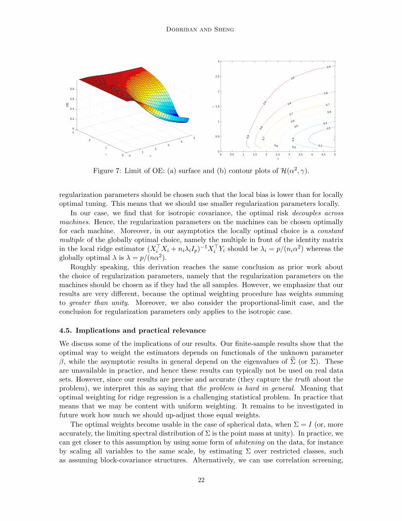
See Appendix F.9 for the proof and Figure 7 for some plots. This proposition impliesthat, for the identity covariance case, the efficiency loss of the distributed estimator in termsof the test error is always less than the loss in terms of the estimation error. When thesignal-to-noise ratio α2 is small, the relative efficiency is always very large and close to 1.This observation can be an encouragement to use our distributed methods for out-of-sampleprediction.

4.4. Choosing the regularization parameter

Previous work found that, under certain conditions, the regularization parameters on theindividual machines should be chosen as if they had the all samples (Zhang et al., 2015).Our findings are consistent with these results. However, the reasons behind our findingsare very different from prior work. The intuition for the previous results is that the vari-ance of distributed estimators averages out, while the bias does not do so. Therefore, the

21

Dobriban and Sheng

03

0.2

0.4

5

OE

2

0.6

4

0.8

31 2

10 0

0.3

0.3

0.4

0.4

0.5

0.5

0.6

0.6

0.6

0.7

0.7

0.7

0.8

0.8

0.8

0.9

0.9

0.9

0.9

0 0.5 1 1.5 2 2.5 3 3.5 4 4.5 50

0.5

1

1.5

2

2.5

3

Figure 7: Limit of OE: (a) surface and (b) contour plots of H(α2, γ).

regularization parameters should be chosen such that the local bias is lower than for locallyoptimal tuning. This means that we should use smaller regularization parameters locally.

In our case, we find that for isotropic covariance, the optimal risk decouples acrossmachines. Hence, the regularization parameters on the machines can be chosen optimallyfor each machine. Moreover, in our asymptotics the locally optimal choice is a constantmultiple of the globally optimal choice, namely the multiple in front of the identity matrixin the local ridge estimator (X>i Xi + niλiIp)

−1X>i Yi should be λi = p/(niα2) whereas the

globally optimal λ is λ = p/(nα2).

Roughly speaking, this derivation reaches the same conclusion as prior work aboutthe choice of regularization parameters, namely that the regularization parameters on themachines should be chosen as if they had the all samples. However, we emphasize that ourresults are very different, because the optimal weighting procedure has weights summingto greater than unity. Moreover, we also consider the proportional-limit case, and theconclusion for regularization parameters only applies to the isotropic case.

4.5. Implications and practical relevance

We discuss some of the implications of our results. Our finite-sample results show that theoptimal way to weight the estimators depends on functionals of the unknown parameterβ, while the asymptotic results in general depend on the eigenvalues of Σ (or Σ). Theseare unavailable in practice, and hence these results can typically not be used on real datasets. However, since our results are precise and accurate (they capture the truth about theproblem), we interpret this as saying that the problem is hard in general. Meaning thatoptimal weighting for ridge regression is a challenging statistical problem. In practice thatmeans that we may be content with uniform weighting. It remains to be investigated infuture work how much we should up-adjust those equal weights.

The optimal weights become usable in the case of spherical data, when Σ = I (or, moreaccurately, the limiting spectral distribution of Σ is the point mass at unity). In practice, wecan get closer to this assumption by using some form of whitening on the data, for instanceby scaling all variables to the same scale, by estimating Σ over restricted classes, suchas assuming block-covariance structures. Alternatively, we can use correlation screening,

22


where we remove features with high correlation. At this stage, all these approaches areheuristic, but we include them to explain how our results can be relevant in practice. It isa topic of future research to make these ideas more concrete. In the algorithm we proposedin Section 5, we use grid search to find a good tuning parameter under general covariancestructures.

On the theoretical side, our results can also be interpreted as a form of reduction betweenstatistical problems. If we can estimate the quadratic functionals of the unknown regressionparameter involved in our weights, then we can do optimally weighted ridge regression.In this sense, we reduce distributed ridge regression to the estimation of those quadraticfunctionals. We think that in the challenging and novel setting of distributed learning, suchreductions can be both interesting and potentially useful.

An important question is “Should we use distributed linear or ridge regression?”. If wehave ni ≥ p and linear regression is defined on each local machine, then we can use eitherdistributed linear (Dobriban and Sheng, 2018) or ridge regression. Linear regression hasthe advantage that the optimal weights are easy to find. Therefore, if we cannot reasonablyreduce to the case Σ = I, it seems we should use linear regression.

4.6. Minimax optimality of the optimal distributed estimator

To deepen our understanding of the distributed problem, we next show that the optimaldistributed ridge estimator is asymptotically rate-minimax. Suppose without loss of gener-ality that the noise level σ2 = 1, and let Sp−1(α) = {β ∈ Rp; ||β|| = α} denote the sphereof radius α ≥ 0 in Rp centered at the origin. Then the minimax risk for estimating β overthe sphere Sp−1(α) is

r(α) = infβ

supβ∈Sp−1(α)

R(β, β) = infβ

supβ∈Sp−1(α)

Eβ||β − β||2,

where the expectation is over both X and ε. This problem has been well studied by Dicker(2016), who reduced it to the following Bayes problem. Let π be the uniform measure onSp−1(α). Then the Bayes risk with respect to π is

rB(α) = infβ

∫Sp−1(α)

R(β, β)dπ(β) = infβ

Eπ||β − β||2.

The Bayes estimator is the posterior mean βSp−1(α) = Eπ(β|y,X). So the corresponding

Bayes risk is rB(α) = Eπ||βSp−1(α) − β||2. Then, the Bayes estimator also minimizes theoriginal minimax risk and r(α) = rB(α) (Dicker, 2016).

Recall that the ridge estimator with optimally tuned regularization parameter is

βr(α) = (X>X +p

α2Ip)−1X>Y,

which can be interpreted as the posterior mean of β under the normal prior assumptionβ ∼ N (0, α2/pIp). When p is very large, the normal distribution N (0, α2/pIp) is very close

to the uniform distribution on Sp−1(α), so we would expect that βSp−1(α) ≈ βr(α). Withthis intuition, Dicker (2016) further showed that, as p, n → ∞, p/n → γ ∈ (0,∞), for anyβ ∈ Sp−1(α)

limn,p→∞

[R(βSp−1(α), β)−R(βr(α), β)

]= 0.

23

Dobriban and Sheng

So the global ridge estimator is asymptotically exact minimax.We call an estimator is asymptotically rate-minimax if asymptotically its risk is at most

a constant times the minimax risk. For our distributed problem, we have the followingresult:

Theorem 10 (Minimax optimality) For fixed signal strength α2, the optimally weighteddistributed ridge estimator is asymptotically rate minimax. Specifically, its risk Mk is lessthan the risk M1 of the global ridge estimator multiplied by a constant C = 1 + α2 whichonly depends on the signal strength α2, and not on the aspect ratio γ = lim p/n and numberof machines k. Specifically

Mk ≤ (1 + α2)M1.

Moreover, for fixed aspect ratio γ > 1, the distributed risk Mk is less than the global riskM1 times a constant C ′ = γ2/(γ2 − 1) which is independent of α2 and k, i.e.

Mk ≤γ2

γ2 − 1M1.

Therefore, in either case, the optimally weighted distributed ridge estimator is asymptoticallyrate minimax.

See Section F.10 for the proof. The minimax optimality result is nontrivial, and doesnot hold for some simpler estimators. For instance, for the null estimator βnull = 0, thecorresponding ARE can be written in terms of the optimal risk function φ(γ) as

limn,p→∞

R(βr(α), β)

R(βnull, β)=φ(γ)

α2=γmγ(−γ/α2)

α2.

When γ → ∞, we know that γ/α2mγ(−γ/α2) → 1, so that even the null estimator isasymptotically exact minimax. In this regime, exact minimaxity is a weak result. Whenγ → 0 however, we have γ/α2mγ(−γ/α2)→ 0 for any α, and so the null estimator does notperform well (has zero efficiency). However, the distributed estimator is still asymptoticallyrate-minimax.

5. WONDER: Algorithms for Weighted One-shot Distributed RidgeRegression

So far, most of our results on distributed ridge regression are purely theoretical. In practice,it would be very helpful to have an implementable algorithm. In fact, our theory fordistributed ridge regression allows us to develop an efficient algorithm which works fordesigns X with arbitrary covariance structures Σ.

Recall that we have n samples distributed across k machines. For simplicity, let usassume the samples are equally distributed. On the i-th machine, we compute a local ridgeestimator βi, local estimators σ2

i , α2i of the signal-to-noise ratio and the noise level. From

Theorem 3, we know that the other quantities needed to find the optimal weights are m,m′

and λ. For m and m′, by the definition of the Stieltjes transform, they can be approximatedby

tr[(Σi + λI)−1]

p≈ m(−λ) and

tr[(Σi + λI)−2]

p≈ m′(−λ).

24


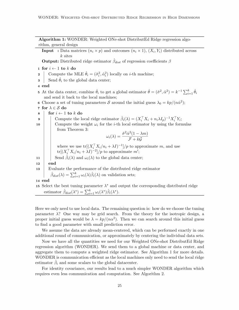
Algorithm 1: WONDER: Weighted ONe-shot DistributEd Ridge regression algo-rithm, general design

Input : Data matrices (ni × p) and outcomes (ni × 1), (Xi, Yi) distributed acrossk sites

Output: Distributed ridge estimator βdist of regression coefficients β

1 for i← 1 to k do

2 Compute the MLE θi = (σ2i , α

2i ) locally on i-th machine;

3 Send θi to the global data center;

4 end

5 At the data center, combine θi to get a global estimator θ = (σ2, α2) = k−1∑k

i=1 θiand send it back to the local machines;

6 Choose a set of tuning parameters S around the initial guess λ0 = kp/(nα2);7 for λ ∈ S do8 for i← 1 to k do

9 Compute the local ridge estimator βi(λ) = (X>i Xi + niλIp)−1X>i Yi;

10 Compute the weight ωi for the i-th local estimator by using the formulasfrom Theorem 3:

ωi(λ) =σ2α2(1− λm)

F + kGwhere we use tr[(X>i Xi/ni + λI)−1]/p to approximate m, and usetr[(X>i Xi/ni + λI)−2]/p to approximate m′;

11 Send βi(λ) and ωi(λ) to the global data center;

12 end13 Evaluate the performance of the distributed ridge estimator

βdist(λ) =∑k

i=1 ωi(λ)βi(λ) on validation sets;

14 end15 Select the best tuning parameter λ∗ and output the corresponding distributed ridge

estimator βdist(λ∗) =

∑ki=1 ωi(λ

∗)βi(λ∗).

Here we only need to use local data. The remaining question is: how do we choose the tuningparameter λ? One way may be grid search. From the theory for the isotropic design, aproper initial guess would be λ = kp/(nα2). Then we can search around this initial guessto find a good parameter with small prediction error.

We assume the data are already mean-centered, which can be performed exactly in oneadditional round of communication, or approximately by centering the individual data sets.

Now we have all the quantities we need for our Weighted ONe-shot DistributEd Ridgeregression algorithm (WONDER). We send them to a global machine or data center, andaggregate them to compute a weighted ridge estimator. See Algorithm 1 for more details.WONDER is communication efficient as the local machines only need to send the local ridgeestimator βi and some scalars to the global datacenter.

For identity covariance, our results lead to a much simpler WONDER algorithm whichrequires even less communication and computation. See Algorithm 2.

25

Dobriban and Sheng

Algorithm 2: WONDER: Weighted ONe-shot DistributEd Ridge regression algo-rithm, isotropic design

Input : Data matrices (ni × p) and outcomes (ni × 1), (Xi, Yi) distributed acrossk sites

Output: Distributed ridge estimator βdist of regression coefficients β

1 for i← 1 to k do

2 Compute the MLE θi = (σ2i , α

2i ) locally on i-th machine;

3 Set local aspect ratio γi = p/ni;4 Set regularization parameter λi = γi/α

2i ;

5 Compute the local ridge estimator βi(λi) = (X>i Xi + niλiIp)−1X>i Yi;

6 Send θi, γi and βi to the global data center.

7 end

8 At the data center, combine θi to get a global estimator θ = (σ2, α2), by

θ = k−1∑k

i=1 θi;9 Evaluate the optimal risk functions for i = 1, 2, . . . , k

φ(γi) = γimγi(−γi/α2) =−γi/α2 + γi − 1 +

√(−γi/α2 + γi − 1)2 + 4γ2

i /α2

2γi/α2;

10 Compute the optimal weights ω, where the i-th coordinate of ω is

ωi =

(α2

φ(γi)

)·

1

1 +∑k

i=1

[α2

φ(γi)− 1] ;

11 Output the distributed ridge estimator βdist =∑k

i=1 ωiβi.

In the above WONDER algorithms, we combine the local estimators of the noise leveland signal strength θi to find a global estimator θ. A simple method is to take the aver-age: θ = k−1

∑ki=1 θi. Another option is to use inverse-variance weighting, based on the

asymptotic variance of the MLE (which then of course has to be estimated).

Based on the results so far, it follows that our WONDER algorithm can consistentlyestimate the limiting optimal weights, and moreover it has asymptotically optimal meansquared error among all weighted distributed ridge estimators, at least for the identitycovariance case. We omit the details.

6. Experimental Results

We present some numerical results in addition to the ones already shown in the paper.

26


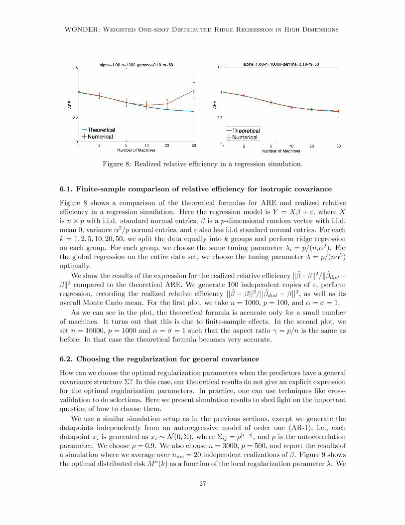
Figure 8: Realized relative efficiency in a regression simulation.

6.1. Finite-sample comparison of relative efficiency for isotropic covariance

Figure 8 shows a comparison of the theoretical formulas for ARE and realized relativeefficiency in a regression simulation. Here the regression model is Y = Xβ + ε, where Xis n× p with i.i.d. standard normal entries, β is a p-dimensional random vector with i.i.d.mean 0, variance α2/p normal entries, and ε also has i.i.d standard normal entries. For eachk = 1, 2, 5, 10, 20, 50, we split the data equally into k groups and perform ridge regressionon each group. For each group, we choose the same tuning parameter λi = p/(niα

2). Forthe global regression on the entire data set, we choose the tuning parameter λ = p/(nα2)optimally.

We show the results of the expression for the realized relative efficiency ‖β−β‖2/‖βdist−β‖2 compared to the theoretical ARE. We generate 100 independent copies of ε, performregression, recording the realized relative efficiency ||β − β||2/||βdist − β||2, as well as itsoverall Monte Carlo mean. For the first plot, we take n = 1000, p = 100, and α = σ = 1.

As we can see in the plot, the theoretical formula is accurate only for a small numberof machines. It turns out that this is due to finite-sample effects. In the second plot, weset n = 10000, p = 1000 and α = σ = 1 such that the aspect ratio γ = p/n is the same asbefore. In that case the theoretical formula becomes very accurate.

6.2. Choosing the regularization for general covariance

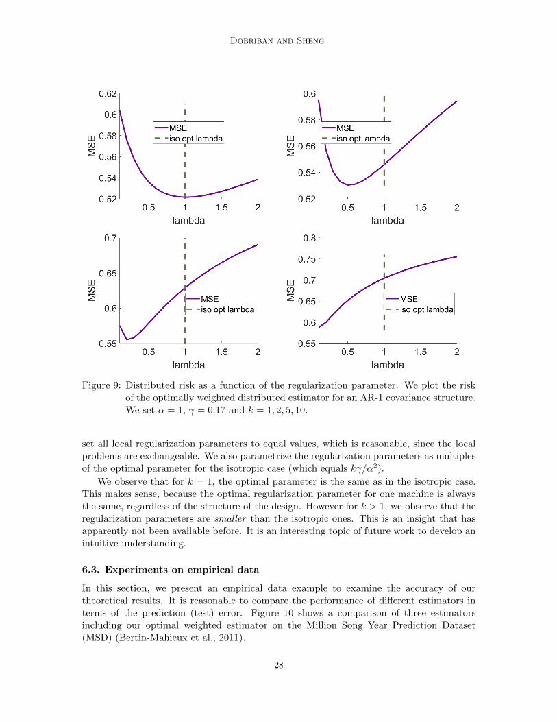
How can we choose the optimal regularization parameters when the predictors have a generalcovariance structure Σ? In this case, our theoretical results do not give an explicit expressionfor the optimal regularization parameters. In practice, one can use techniques like cross-validation to do selections. Here we present simulation results to shed light on the importantquestion of how to choose them.

We use a similar simulation setup as in the previous sections, except we generate thedatapoints independently from an autoregressive model of order one (AR-1), i.e., eachdatapoint xi is generated as xi ∼ N (0,Σ), where Σij = ρ|i−j|, and ρ is the autocorrelationparameter. We choose ρ = 0.9. We also choose n = 3000, p = 500, and report the results ofa simulation where we average over nmc = 20 independent realizations of β. Figure 9 showsthe optimal distributed risk M∗(k) as a function of the local regularization parameter λ. We

27

Dobriban and Sheng

Figure 9: Distributed risk as a function of the regularization parameter. We plot the riskof the optimally weighted distributed estimator for an AR-1 covariance structure.We set α = 1, γ = 0.17 and k = 1, 2, 5, 10.

set all local regularization parameters to equal values, which is reasonable, since the localproblems are exchangeable. We also parametrize the regularization parameters as multiplesof the optimal parameter for the isotropic case (which equals kγ/α2).

We observe that for k = 1, the optimal parameter is the same as in the isotropic case.This makes sense, because the optimal regularization parameter for one machine is alwaysthe same, regardless of the structure of the design. However for k > 1, we observe that theregularization parameters are smaller than the isotropic ones. This is an insight that hasapparently not been available before. It is an interesting topic of future work to develop anintuitive understanding.

6.3. Experiments on empirical data

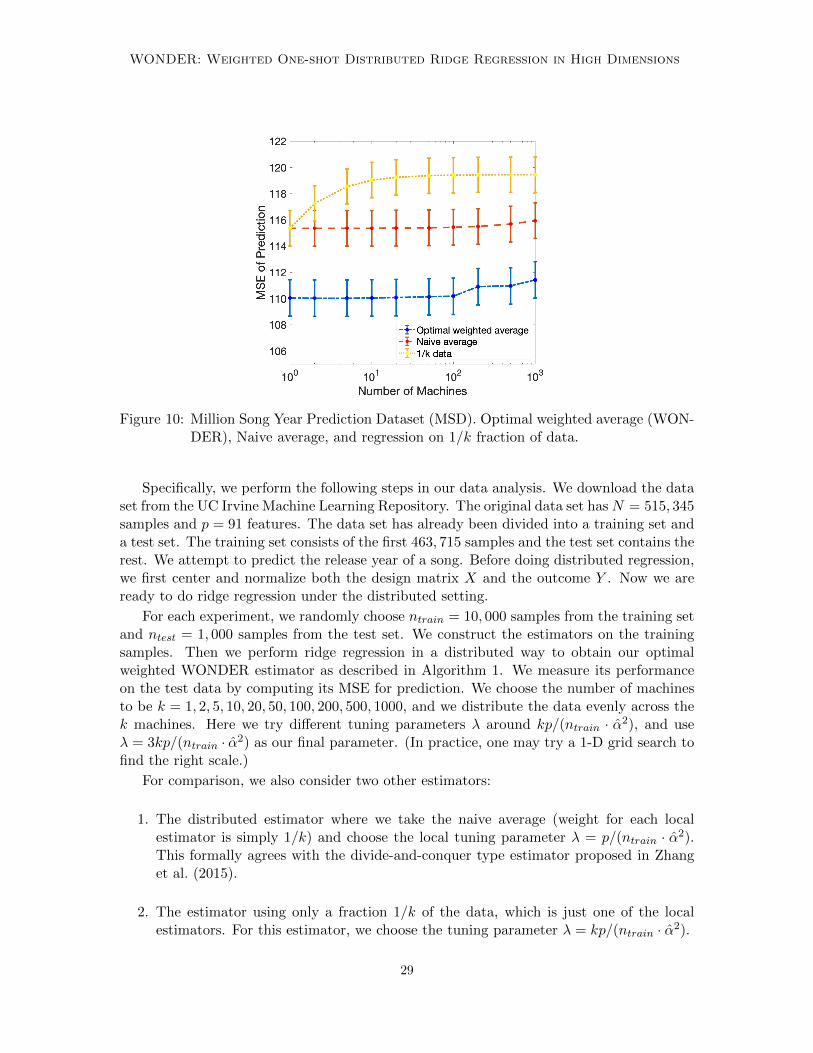
In this section, we present an empirical data example to examine the accuracy of ourtheoretical results. It is reasonable to compare the performance of different estimators interms of the prediction (test) error. Figure 10 shows a comparison of three estimatorsincluding our optimal weighted estimator on the Million Song Year Prediction Dataset(MSD) (Bertin-Mahieux et al., 2011).

28


Figure 10: Million Song Year Prediction Dataset (MSD). Optimal weighted average (WON-DER), Naive average, and regression on 1/k fraction of data.

Specifically, we perform the following steps in our data analysis. We download the dataset from the UC Irvine Machine Learning Repository. The original data set hasN = 515, 345samples and p = 91 features. The data set has already been divided into a training set anda test set. The training set consists of the first 463, 715 samples and the test set contains therest. We attempt to predict the release year of a song. Before doing distributed regression,we first center and normalize both the design matrix X and the outcome Y . Now we areready to do ridge regression under the distributed setting.

For each experiment, we randomly choose ntrain = 10, 000 samples from the training setand ntest = 1, 000 samples from the test set. We construct the estimators on the trainingsamples. Then we perform ridge regression in a distributed way to obtain our optimalweighted WONDER estimator as described in Algorithm 1. We measure its performanceon the test data by computing its MSE for prediction. We choose the number of machinesto be k = 1, 2, 5, 10, 20, 50, 100, 200, 500, 1000, and we distribute the data evenly across thek machines. Here we try different tuning parameters λ around kp/(ntrain · α2), and useλ = 3kp/(ntrain · α2) as our final parameter. (In practice, one may try a 1-D grid search tofind the right scale.)

For comparison, we also consider two other estimators:

1. The distributed estimator where we take the naive average (weight for each localestimator is simply 1/k) and choose the local tuning parameter λ = p/(ntrain · α2).This formally agrees with the divide-and-conquer type estimator proposed in Zhanget al. (2015).

2. The estimator using only a fraction 1/k of the data, which is just one of the localestimators. For this estimator, we choose the tuning parameter λ = kp/(ntrain · α2).

29

Dobriban and Sheng

We repeat the experiment for T = 100 times, and report the average and 1/4 standarddeviation over all experiments on Figure 10. Each time we randomly collect new trainingand test sets.

From Figure 10, we observe the following:

1. The WONDER estimator has smaller MSE than both the local estimator and thenaive averaged estimator, which means optimal weighting can indeed help.

2. It seems that data splitting does not have huge impact on the performance of theWONDER estimator. This phenomenon is compatible with our theory. Since thesignal-to-noise ratio α2 is about 1.2 for this data set, we are in a low SNR scenario.From Proposition 9 and Figure 7, we see that the performance of the distributedestimator is close to the global estimator in terms of the prediction error.

To conclude, in terms of computation-statistics tradeoff, this example suggests a verypositive outlook on using distributed ridge regression via WONDER: The accuracy is af-fected very little even though the data is split up into 100 parts. Thus we save at least 100xin computation time, while we have nearly no loss in performance.

Finally, we mention that in Figure 4 of Zhang et al. (2015), the authors also compare theperformance of the distributed estimator to the local estimator on the same Million Songdata set. We notice that the MSE of prediction in their experiments is usually between80 and 90, and variance is typically very small. In our experiments, both the MSE andvariance are larger. The reason for this seems to be that they consider more general kernelridge regression.

Acknowledgments

The authors are very grateful to the Action Editor and the referees for their work in editingand reviewing the paper. The authors thank Yuekai Sun for discussions motivating ourstudy, as well as John Duchi, Jason D. Lee, Xinran Li, Jonathan Rosenblatt, Feng Ruan,and Linjun Zhang for helpful discussions. They are grateful to Sifan Liu for thoroughcomments on an earlier version of the manuscript. They are also grateful to the associateeditor and referees for valuable suggestions. ED was partially supported by NSF BIGDATAgrant IIS 1837992.

Appendix A. Adding a Constant to the Regression

We show below the details of the derivation of optimal weights for ridge regression whenwe also add a constant to the (biased) local estimators. In our calculation from Theorem1, we need to change some details as follows:

We need to define a new matrix B = [β1, . . . , βk, p−1/21p] and new weights w = [w;wk+1].

Clearly, we still have that

B = [Eβ1, . . . ,Eβk, p−1/21p] = [Q1β; . . . ;Qkβ, p−1/21p].

The new matrix R is now diagonal with all entries as before, and the lower right cornerentry is Rk+1 = 0.

30


We consider the same regression problem as before, except we add an intercept into thematrix B as above. The same algebraic form of the optimal weights and risk holds, withthe new definitions above. The optimal risk is now

M∗(k) = ‖β‖2 − v>(A+R)−1v

where

v = B>β = [vec[β>Qiβ]; p−1/21>p β]

A =

[mx[β>QiQjβ] vec[p−1/21>p Qiβ]

vec[p−1/21>p Qiβ] 1

]R = diag

[n−1i tr[(Σi + λiIp)

−2Σi]; 0]

Qi = (Σi + λiIp)−1Σi

In simulation studies, we have observed that this approach typically does not lead to asignificant decrease in MSE.

Appendix B. Differentiation Rule for Calculus of DeterministicEquivalents

Theorem 11 (Differentiation rule) Suppose T = Tn and S = Sn are two (deterministicor random) matrix sequences of growing dimensions such that f(z, Tn) � g(z, Sn), wherethe entries of f and g are analytic functions in z ∈ D and D is an open connected subsetof C. Suppose that for any sequence Cn of deterministic matrices with bounded trace normwe have

| tr [Cn(f(z, Tn)− g(z, Sn))] | ≤M

for every n and z ∈ D. Then we have f ′(z, Tn) � g′(z, Sn) for z ∈ D, where the derivativesare entry-wise with respect to z.

To prove this theorem, we need to introduce a lemma from complex analysis which is aconsequence of the dominated convergence theorem and Cauchy’s integral formula.

Lemma 12 (see Lemma 2.14 in Bai and Silverstein (2010)) Let f1, f2, . . . be ana-lytic on the domain D, satisfying |fn(z)| ≤ M for every n and z ∈ D. Suppose that thereis an analytic function on D such that fn(z)→ f(z) for all z ∈ D. Then it also holds thatf ′n(z)→ f ′(z) for all z ∈ D.

The proof of theorem 11 is clear. Since tr [Cn(f(z, Tn)− g(z, Sn))] is a sequence ofanalytic functions on D with uniform bound, then from the definition of the deterministicequivalence, we have tr [Cn(f(z, Tn)− g(z, Sn))] → 0. By lemma 12, the derivative alsoconverges to 0 for all z ∈ D, which finishes the proof.

31

Dobriban and Sheng

Appendix C. Gaussian MLE for Signal and Noise Components

Recall that our model is Y = Xβ + ε where β and ε are independent. Let θ = (σ2, α2) anddefine the Gaussian log-likelihood,

`(θ) = −1

2log(σ2)− 1

2nlog det

(α2

pXX> + I

)− 1

2σ2nY >

(α2

pXX> + I

)−1

Y.

Note that `(θ) is the log-likelihood for θ under the Gaussian assumption of β ∼ N (0, (σ2α2/p)I)and ε ∼ N (0, σ2I). For the MLE

θ = (σ2, α2) = argmaxσ2,α2≥0

`(θ),

we have the following result from Dicker and Erdogdu (2017).

Theorem 13 (Consistency and asymptotic normality, Dicker and Erdogdu (2017))Suppose θ = (σ2, α2) are the true parameters, then θ → θ in probability as p/n → γ. Fur-thermore, define the Fisher information matrix for θ under the Gaussian assumption model

In(θ) =

[I2(θ) I3(θ)I3(θ) I4(θ)

],

where

Ik(θ) =1

2nσ8−2ktr

[(1

pXX>

)k−2(α2

pXX> + I

)2−k], k = 2, 3, 4.

Then n1/2In(θ)1/2(θ − θ)→ N (0, I2) in distribution as p/n→ γ.

In addition, if we put some assumptions on X as we did in Theorem 1 and denote thelimiting spectral distribution of p−1XX> by Fγ , then the entries of the Fisher informationmatrix In(θ) have limits

Ik(θ)→a.s. Jk(θ) =1

2σ8−2k

∫ (s

α2s+ 1

)k−2

dFγ(s), k = 2, 3, 4.

Thus In(θ) converges almost surely to a limiting information matrix I(θ) which character-izes the asymptotic variance of the MLE θ.

Appendix D. Explaining Decoupling via Free Probability Theory

In this section, we provide an explanation via free probability theory for why the limitingdistributed risk decouples. Specifically, we explain why the limit of the quantities β>Qiβ ·β>Qjβ for i 6= j becomes a product of terms depending on i, j.

We will use some basic notions from free probability theory (Voiculescu et al., 1992;Hiai and Petz, 2006; Nica and Speicher, 2006; Anderson et al., 2009; Couillet and Debbah,2011). Let us define our non-commutative probability space as(

A = (L∞− ⊗Mp(R)), τ =1

ptr

),

32


where L∞− denotes the collection of random variables with all moments finite and Mp(R) isthe space of p×p real matrices. Recall that, a sequence of random variables {a1,p, a2,p, . . . , ak,p} ⊂A is said to be asymptotically free almost surely if

τ [m∏j=1

Pj(aij ,p − τ(Pj(aij ,p)))]→a.s. 0,

for any positive integer m, any polynomials P1, . . . , Pm and any indices i1, . . . , im ∈ [k] withno two adjacent ij equal. Suppose Ap, Bp are two sequences of independent random matricesand at least one of them is orthogonally invariant, then it is well-known that {Ap, Bp} ⊂ Ais asymptotically free almost surely.

Now, let us assume that X>X is orthogonally invariant, which is the case when X>Xfollows the white Wishart distribution. Then clearly X>i Xi and X>j Xj are asymptoticallyfree almost surely. It follows that Qi and Qj are also asymptotically free almost surely. Byusing the definition of asymptotic freeness, we have for i 6= j

τ [(Qi −1

ptr(Qi)I)(Qj −

1

ptr(Qj)I)]→a.s. 0,

which is equivalent to

1

ptr(QiQj)−

1

ptr(Qi)

1

ptr(Qj)→a.s. 0.

Hence, under the random-effects assumption for β, the limit of β>β · β>QiQjβ (i 6= j) willdecouple and is the same as the limit of β>Qiβ · β>Qjβ.

Appendix E. Intuitive Explanation for the Need to Use WeightsSumming to Greater than Unity

Consider a much more simplified problem, where we are estimating a scalar parameter θ.We have an estimator θ, which is generally biased, and we would like to find the scalemultiple c · θ that minimizes the mean squared error. A calculation reveals that

M(c) = E(c · θ − θ)2 = c2E(θ2)− 2c · Eθ · θ + θ2

Hence the optimal scale factor is c = Eθ · θ/E(θ2).

We can achieve a better understanding of this optimal scale if we consider the bias-variance decomposition of θ. Let us define the bias and the variance as

B = Eθ − θV = E(θ − Eθ)2

We then see that the optimal scale factor is

c =B + θ

V + (B + θ)2θ = 1− V +B(B + θ)

V + (B + θ)2.

33

Dobriban and Sheng

This quantity is an “inflation factor”, i.e., greater than or equal to unity, if V +B(B+θ) ≤ 0.This can be written as

V +B2 ≤ −Bθ

Hence, this condition can only hold if the bias B has opposite sign with θ. This would bethe case for a shrinkage estimator θ. In that case, the condition could hold if the parameterθ has a large magnitude.

Returning to our main problem, ridge regression is a shrinkage estimator, and averagesof ridge regression estimators are still shrinkage estimators. Therefore, it makes sense thattheir weighted average should be inflated to minimize mean squared error. This providesan intuitive explanation for why the weights sum to greater than one.

Appendix F. Proofs

F.1. Proof of Theorem 1

We can calculate the MSE of the weighted sum as

M(w) = E∥∥∥∑wiβi − β

∥∥∥2= E(

∑wiβi − β)>(

∑wj βj − β)

=∑ij

wiwj · Eβ>i βj − 2∑i

wiEβ>i β + ‖β‖2.

Let B be the p× k matrix defined as B = [β1, . . . , βk]. Then we can write the above MSEas

M(w) = w>EB>Bw − 2Eβ>Bw + ‖β‖2.

Let alsoB = EB = [Eβ1, . . . ,Eβk].

Since the local estimators are independent, we can write

M(w) = w>(B>B +R)w − 2β>Bw + ‖β‖2,

where R is a diagonal matrix with entries

Ri = E‖βi‖2 − ‖Eβi‖2 = E‖βi − Eβi‖2.

The objective function M(w) can be viewed as corresponding to a k-parameter linear re-gression problem, with unknown parameters wi, design matrix B and outcome vector β.Specifically, we regress β on EB = E[β1, . . . , βk]. Therefore, the optimal weights are

w∗ = (B>B +R)−1B>β,

and the optimal risk equals

M∗ = M(w∗) = β>[Ip −B(B>B +R)−1B>

]β.

34


Now, to find B = EB, we need Eβi. The expectation of the ridge regression estimator forthe full data set is

Eβ(λ) = E(X>X + nλIp)−1X>Y = (X>X + nλIp)

−1X>Xβ.

Letting Σ = n−1X>X, this equals Eβ(λ) = (Σ + λIp)−1Σβ. Similarly,

Eβi(λi) = (X>i Xi + niλiIp)−1X>i Xiβ.

Let Qi = Qi(λi) = (X>i Xi + niλiIp)−1X>i Xi be those matrices and let Σi = n−1X>i Xi.

Then the above equals Qi = (Σi + λiIp)−1Σi, and

B = [Q1β; . . . ;Qkβ].

Therefore, B>B has entries β>QiQjβ, while B>β has entries β>Qiβ. Moreover,

Ri = E‖βi − Eβi‖2 = E‖(X>i Xi + niλiIp)−1X>i εi‖2 = σ2 tr[(X>i Xi + niλiIp)

−2X>i Xi].

We can also write this as Ri = n−1i σ2 tr[(Σi + λiIp)

−2Σi]. To conclude the optimal risk, wehave

M∗(k) = ‖β‖2 − v>(A+R)−1v,

where

v = B>β = vec[β>Qiβ],

A = mat[β>QiQjβ],

R = diag[n−1i σ2 tr[(Σi + λiIp)

−2Σi]],

Qi = (Σi + λiIp)−1Σi.

Here we used the vectorization and to-matrix operators vec,mat. For the global MSE, weonly need to consider the special case where k = 1, which gives us

E||β − β||2 = M∗(1) = ‖β‖2 − (β>Qβ)2

β>Q2β + σ2 tr[(X>X + nλIp)−2X>X],

where Q = (Σ + λIp)−1Σ. This finishes the argument.


The first step is to use the well-known concentration of quadratic forms to reduce to tracefunctionals (See e.g. Lemma C.3 of Dobriban and Wager (2018) which is based on LemmaB.26 of Bai and Silverstein (2010)). Since β is independent of the data X with mean zeroand finite variance, under the moment assumptions imposed in the theorem, we have

β>Qiβ − σ2α2/p · trQi →a.s. 0,

β>QiQjβ − σ2α2/p · trQiQj →a.s. 0,

β>Q2iβ − σ2α2/p · trQ2

i →a.s. 0.

Let us compute the limits of v,A and R respectively.

35

Dobriban and Sheng

1. Limit of v: First of all, we have already known that

β>Qiβ − σ2α2/p · trQi →a.s. 0,

so it is sufficient to consider the limit of trQi/p. Since

trQi/p = 1− λi tr[(Σi + λiIp)−1]/p.

assuming that the spectral distribution of Σi converges almost surely to Fγi , we thushave

trQi/p→a.s. 1− λiEFγi (T + λi)−1 = 1− λimFγi

(−λi).

Above we have introduced the Stieltjes transform mFγias a limiting object. So,

β>Qiβ →a.s. σ2α2[1− λimFγi

(−λi)].

For the form in terms of the population spectral distribution H, if p/n → γ and thespectral distribution of Σ converges to H, we have by the general Marchenko-Pastur(MP) theorem of Rubio and Mestre (Rubio and Mestre, 2011), that

(Σ + λI)−1 � (xpΣ + λI)−1,

where xp is the unique positive solution of the fixed point equation

1− xp =xpn

tr[Σ(xpΣ + λI)−1

].

When n, p→∞, xp → x and x satisfies the equation

1− x = γ

[1− λ

∫ ∞0

dH(t)

xt+ λ

].

We remark that the assumptions made in the theorem suffice for using the Rubio-Mestre result. Moreover, we only use a special case of their result, similar to Dobribanand Sheng (2018). Hence from the calculus of deterministic equivalents (Dobriban andSheng, 2018), we can take the traces of the matrices in question to obtain

trQi/p = 1− λi tr[(Σi + λiIp)−1]/p � 1− λi tr[(xiΣ + λiI)−1]/p→a.s. EH

xiT

xiT + λi,

where xi = x(H, γi,−λi) is the unique solution of

1− xi = γi

[1− λi

∫ ∞0

dH(t)

xit+ λi

].

2. Limit of A: Let us consider the cases i 6= j and i = j separately.

36


(a) i 6= j: We begin by

β>QiQjβ − σ2α2/p · trQiQj →a.s. 0.

Based on the above expression for Qi, we have

QiQj = Ip−λi(Σi+λiIp)−1−λj(Σj +λjIp)

−1 +λiλj(Σi+λiIp)−1(Σj +λjIp)

−1.

So the key will be to find the limit of

Eij = p−1 tr{(Σi + λiIp)−1(Σj + λjIp)

−1}.

From the general MP theorem, since p/ni → γi, we have for all i,

(Σi + λiIp)−1 � (xipΣ + λiIp)

−1.

Here xip is the unique positive solution of the fixed point equation

1− xip =xipni

tr[Σ(xipΣ + λiI)−1

],

and xip → xi as ni, p→∞. By the product rule of the calculus of deterministicequivalents, we have for i 6= j

(Σi + λiIp)−1(Σj + λjIp)

−1 � (xipΣ + λiIp)−1(xjpΣ + λjIp)

−1.

Hence by the trace rule of deterministic equivalents,

Eij � p−1 tr[(xipΣ + λiIp)−1(xjpΣ + λjIp)

−1]

Moreover, since the spectral distribution of Σ converges to H, we find for i 6= j

Eij → EH1


Putting it together,

QiQj � Ip−λi(xipΣ+λiIp)−1−λj(xjpΣ+λjIp)

−1+λiλj(xipΣ+λiIp)−1(xjpΣ+λjIp)

−1.

So, again by the trace rule of deterministic equivalents, we have

p−1 tr{QiQj} →a.s. 1− EHλi

xiT + λi− EH

λjxjT + λj

+ EHλiλj

(xiT + λi)(xjT + λj)

= xixjEHT 2


Therefore, for i 6= j

Aij → σ2α2

[xixjEH

T 2


].

37

Dobriban and Sheng

(b) i = j: In this case,β>Q2

iβ − σ2α2/p · trQ2i → 0,

where Q2i = Ip − 2λi(Σi + λiIp)

−1 + λ2i (Σi + λiIp)

−2. We can easily find thelimit of trQ2

i /p in terms of empirical quantities, based on our knowledge of theconvergence of Stieltjes transforms and its derivatives:

trQ2i /p→ 1− 2λimFγi

(−λi) + λ2im′Fγi

(−λi).

Therefore, for i = j

Aii → σ2α2[1− 2λimFγi(−λi) + λ2

im′Fγi

(−λi)].

We can also express the limit of Aii in terms of the population spectral distribu-tion H by using Theorem 11. For our purpose, let T = Σ, S = Σ, while

f(z, T ) = (xpT − zI)−1,

g(z, S) = (S − zIp)−1.

From Rubio and Mestre (2011), we know that for each z ∈ D := C\R+, f(z,Σ) �g(z, Σ). xp is defined as

xp =1

ntr[(I +

p

nepI)−1] =

1

1 + (p/n)ep=

1

1 + γpep,

and ep = ep(z) is the Stieltjes transform of a certain positive measure on R+,obtained as the unique solution of the equation

ep =1

ptr[Σ(xpΣ− zIp)−1].

It is well-known that xp(z), ep(z) are both analytic functions on D. Then we cancheck that the conditions of theorem 11 hold in this case. First of all, for aninvertible matrix A, A−1 = (detA)−1A∗, where A∗ is the adjugate matrix of A.Since xp is analytic, it is easy to verify that det(xpΣ− zIp),det(Σ− zIp) and all

entries of (xpΣ − zIp)∗, (Σ − zIp)∗ are analytic functions of z. So the entries of

f(z,Σ) and g(z, Σ) are analytic in D.

Next, we want to bound

tr[Cn((xpΣ− zIp)−1 − (Σ− zIp)−1)] ≤ ||Cn||tr · ||(xpΣ− zIp)−1 − (Σ− zIp)−1||2.

For a fixed δ > 0, let us define a domain Dδ := {z ∈ D : Rez < −δ} ∪ {z ∈ D :|Imz| > δ}. Then, it is sufficient to find a uniform bound for ||(xpΣ − zIp)−1 −(Σ−zIp)−1||2 on Dδ. In fact, we can bound ||(xpΣ−zIp)−1||2 and ||(Σ−zIp)−1||2separately.

i. Bounding ||(Σ− zIp)−1||2:

||(Σ− zIp)−1||2 = σmax((Σ− zIp)−1) = maxi

1

|li − z|,

38


where li is the i-th eigenvalue of Σ. Since li is always non-negative, we have

1

|li − z|=

1

|li − Rez − iImz|=

1√(li − Rez)2 + (Imz)2

≤ 1

δ.

ii. Bounding ||(xpΣ− zIp)−1||2:In this case, we need to use the properties of ep and xp. Recall that ep is theStieltjes transform of a certain measure on R+, i.e.

ep(z) =

∫ ∞0

1

t− zdµ(t) =

∫ ∞0

1

t− Rez − iImzdµ(t)

=

∫ ∞0

t− Rez

(t− Rez)2 + (Imz)2dµ(t) + i

∫ ∞0

Imz

(t− Rez)2 + (Imz)2dµ(t).

So

xp =1

1 + γpep=

1

1 + γpRe(ep) + iγpIm(ep)

=1 + γpRe(ep)

(1 + γpRe(ep))2 + (γpIm(ep))2− i γpIm(ep)

(1 + γpRe(ep))2 + (γpIm(ep))2.

When z ∈ Dδ, we can check that Re(xp) > 0. Meanwhile, Im(xp) and Im(z)have opposite signs.Now, let us consider

||(xpΣ− zIp)−1||2 = σmax((xpΣ− zIp)−1) = maxk

1

|xplk − z|,

where lk is the k-th eigenvalue of Σ. Since lk is non-negative, we have

1

|xplk − z|=

1

|lkRe(xp) + ilkIm(xp)− Rez − iImz|

=1√

(lkRe(xp)− Rez)2 + (lkIm(xp)− Imz)2

≤ 1

δ.

Finally, since δ is arbitrary, we can conclude that f ′(z,Σ) � g′(z, Σ) for all z ∈ D.

Then let us compute the derivatives. For invertible A = A(z), we have

d(A−1)

dz= −A−1dA

dzA−1,

where the derivative is entry-wise. Thus

f ′(z, T ) = −(xpT − zI)−1(x′pT − I)(xpT − zIp)−1 = −(xpT − zIp)−2(x′pT − I),

g′(z, S) = (S − zIp)−2.

39

Dobriban and Sheng

Next, we need to calculate x′ = dx/dz, where x(z) is the limit of xp(z). In fact,by looking at the expression of xp(z), it is not hard to find that xp(z) is uniformlybounded on D. By using a similar argument, we have x′p → x′ on D. To find x′,let us start from the following fixed-point equation

1− x = γ

[1 + zEH

1

xT − z

].

Take derivatives on both sides to get

−x′ = γ

[zEH

1

xT − z

]′−x′ = γ

[EH

1

xT − z+ EH

z − zTx′

(xT − z)2

]x′[−1 + γzEH

T

(xT − z)2

]= γEH

xT

(xT − z)2

x′ =γEH xT

(xT−z)2

−1 + γzEH T(xT−z)2

.

Therefore we obtain

(Σ− zI)−2 � (xpΣ− zIp)−2(I − x′pΣ)

p−1 tr(Σ− zI)−2 � −x′pp−1 tr[Σ(xpΣ− zI)−2] + p−1 tr[(xpΣ− zIp)−2]

→γEH xT

(xT−z)2

1− γzEH T(xT−z)2

EHT

(xT − z)2+ EH

1

(xT − z)2

=γx(EH T

(xT−z)2

)2

1− γzEH T(xT−z)2

+ EH1

(xT − z)2.

Now, let z = −λ and then we will have

(Σ + λI)−2 � (xpΣ + λI)−2(I − x′pΣ)

p−1 tr(Σ + λI)−2 →γx(EH T

(xT+λ)2

)2

1 + γλEH T(xT+λ)2

+ EH1

(xT + λ)2.

Finally, we can simply replace Σ, λ, γ, x by Σi, λi, γi, xi to get the desired results.

3. Limit of R: Recall that Ri = n−1i σ2 tr[(Σi + λiIp)

−2Σi]. We note p−1 tr(Σ + λI)−2 →m′Fγ (−λ) and Σ(Σ + λI)−2 = (Σ + λI)−1 − λ(Σ + λI)−2, so

tr[Σ(Σ + λI)−2]

n→ γ[mFγ (−λ)− λm′Fγ (−λ)].

HenceRii → σ2

[γi[mFγi

(−λi)− λm′Fγi (−λi)]].

40


Next, we find a limit in terms of population parameters

Σ(Σ + λI)−2 = (Σ + λI)−1 − λ(Σ + λI)−2

� (xpΣ + λI)−1 − λ(xpΣ + λI)−2(I − x′pΣ)

p−1 tr Σ(Σ + λI)−2 � p−1 tr(xpΣ + λI)−1 − λp−1 tr[(I − x′pΣ)(xpΣ + λI)−2

]→ EH

1

xT + λ− λ

γx(EH T

(xT+λ)2

)2


− EHλ

(xT + λ)2

= EHxT

(xT + λ)2− λ

γx(EH T

(xT+λ)2

)2


=xEH T

(xT+λ)2

1 + λγEH T(xT+λ)2

,

where we used the differentiation rule of the calculus of deterministic equivalents.Hence we finally find the limit

Rii → σ2

[xiEH T

(xiT+λi)2

1 + λiγiEH T(xiT+λi)2

].


Notice that, when the samples are equally distributed and we use the same tuning parameterλ for all the local estimators, a direct consequence is that xi = xj = x for all i, j, where xis the unique solution of the following fixed point equation

1−x = kγ

[1− λ

∫ ∞0

dH(t)

xt+ λ

]= kγ

[1− EH

λ

xT + λ

]= kγ(1−λmFkγ (−λ)) = kγ(1−λm).

In this case, we can express Aij as

Aij = σ2α2EH(xT )2

(xT + λ)2= σ2α2

∫(xt)2

(xt+ λ)2dH(t).

In order to express Aij in terms of the sample quantities, we can start from the followingequality ∫

1

xt+ λdH(t) = m.

Take derivatives with respect to λ, we have∫x′t+ 1

(xt+ λ)2dH(t) = m′.

Rearrange terms, we have∫x′t+ 1

(xt+ λ)2dH(t) =

∫(xt+ λ− λ) · x′x + 1

(xt+ λ)2dH(t) =

x′

xm+

(1− λx′

x

)∫1

(xt+ λ)2dH(t) = m′.

41

Dobriban and Sheng

On the other hand, take derivatives with respect to λ on the fixed point equation for x givesus

x′ = kγ(m− λm′).

So ∫1

(xt+ λ)2dH(t) =

xm′ − x′mx− λx′

=(1− kγ)m′ + 2kγλmm′ − kγm2

1− kγ + kγλ2m′.

Then we have ∫(xt)2

(xt+ λ)2dH(t) =

∫(xt+ λ− λ)2

(xt+ λ)2dH(t)

= 1− 2λm+ λ2

∫1

(xt+ λ)2dH(t)

= 1− 2λm+ λ2m′ − kγλ2(m− λm′)2

1− kγ + kγλm′.

Now we the expressions for V,A,R, we also know W∗k = (A +R)−1V and Mk = σ2α2 −V >(A+R)−1V . By using the auxiliary functions F ,G defined in the theorem, we have

Mk = σ2α2− 1

GV >(1 · 1>+diag(F/G))−1V = σ2α2−(σ2α2(1− λm))2

G1>(1 · 1>+diag(F/G))−11,

where 1 = (1, 1, · · · , 1)> is the all-one vector. Then similar to the proof of Theorem 2, wecan use the Sherman-Morrison formula to simply the expression, this leads to

Mk = σ2α2 − (σ2α2(1− λm))2

G1>(

diag(F/G)−1 − diag(F/G)−11 · 1> diag(F/G)−1

1 + 1> diag(F/G)−11

)1

= σ2α2 − (σ2α2(1− λm))2

G

(kGF− k2G2/F2

1 + kG/F

)= σ2α2

(1− σ2α2(1− λm)2k

F + kG

).

Similarly, we can express the optimal weights W∗k as

W∗k =1

G(1 · 1> + diag(F/G))−1V

=σ2α2(1− λm)

G(1 · 1> + diag(F/G))−11

=σ2α2(1− λm)

G

(diag(F/G)−1 − G2/F2

1 + kG/F1 · 1>

)1

=σ2α2(1− λm)

F + kG1.

Why do we need to assume the samples are uniformly distributed across machines? Thisis a technical assumption. The key difficulty in analyzing MSE and optimal weights comesfrom the off-diagonal entries of A:

Aij = σ2α2EHxixjT

2


42


Here, xi is uniquely determined by the aspect ratio γi = p/ni, the tuning parameter λi, andthe population distribution H. The terms we can handle are of form

EH(xiT )k

(xiT + λi)l, k, l ∈ N∗.

We can calculate these by taking derivatives of the Stieltjes transform EH 1xiT+λi

and doingfurther calculations.

We may decompose Aij into

Aij = σ2α2

(1− λiEH

1

xiT + λi− λjEH

1

xjT + λj+ λiλjEH

1


).

In general, it is hard to further simplify the last term of the above decomposition. But ifwe assume the subsample sizes are all equal, then the optimal tuning parameters λi shouldalso be equal by symmetry. Thus, all xi are the same and we can rewrite the last term into

λ2iEH

1

(xiT + λi)2,

which is something we can deal with as mentioned above. Besides, from a practical perspec-tive, if the samples are not uniformly distributed, we may need to do much more roundsof communication (compare to Algorithm 1) to find the optimal tuning parameters λi andthe optimal weights ωi.


The proof for v and R is clear by Theorem 2. For the limit of A, the diagonal case is alsodirect. When i 6= j, recall that

Eij = p−1 tr{(Σi + λiIp)−1(Σj + λjIp)

−1} → EH1


For H = δ1, the expectation decouples, we find

Eij →1

xi + λi· 1

xi + λj= mγi(−λi)mγj (−λj).

Therefore,Aij → σ2α2[1− λimγi(−λi)] · [1− λjmγj (−λj)].

Now let us put everything together. Recall that the optimal risk has the form MSE∗dist =‖β‖2 − v>(A+R)−1v. Based on the above discussion, we have

σ2α2(A+R)→ σ2α2(A+R) = V V > +D,

where D is a diagonal matrix with i-th diagonal entry σ2α2(Rii+Aii)−V 2i . Then, by using

the Sherman−Morrison formula, we have

V >(V V > +D)−1V =V >D−1V

1 + V >D−1V.

43

Dobriban and Sheng

So the limiting distributed risk is

Mk = σ2α2 − σ2α2 V >D−1V

1 + V >D−1V=

σ2α2

1 + V >D−1V=

σ2α2

1 +∑k

i=1V 2iDi

,

which finishes the proof.

F.5. Proof of Proposition 5

Recall that

V 2i

Di=

σ4α4(1− λimγi(−λi))2

σ4α4λ2i [m

′γi(−λi)−m2

γi(−λi)] + σ4α2γi[mγi(−λi)− λim′γi(−λi)]

=α2(1− λimγi(−λi))2

α2λ2i [m

′γi(−λi)−m2

γi(−λi)] + γi[mγi(−λi)− λim′γi(−λi)],

and our goal is to find λi that maximizes V 2i /Di. Luckily, from Dobriban and Wager (2018)

it follows that for k = 1, i.e. when there is only one machine, the optimal choice of thetuning parameter λ is γ/α2. This means that the maximizer of V 2/D is λ = γ/α2. Now,due to the decoupled structure of Mk, the optimal tuning parameters are λi = γi/α

2.Plugging in the parameters, we have

V 2i

Di=

α2

γimγi(−γi/α2)− 1.

Then the optimal risk can be simplified to

Mk =σ2α2

1 +∑k

i=1

[α2

γimγi (−γi/α2)− 1] .

When k = 1, this equals to σ2γmγ(−γ/α2) which matches the known result from Dobribanand Wager (2018).


The explicit form is easy to derive by plugging z = −γ/α2 into the formula of mγ(z). Next,we can check monotonicity by computing φ′(γ):

φ′(γ) =α2

2γ2

(1 +

(1− 1/α2)γ − 1√[(1− 1/α2)γ − 1]2 + 4γ2/α2

)> 0.

Finally, for the convexity, let us consider the two cases separately.

1. α ≤ 1: With some effort, we find the second derivative of φ

φ′′(γ) =

α2

(2γ2

α2 −(

((1− 1α2 )γ − 1)2 + 4γ2

α2

) ((1− 1

α2 )γ − 1))−(

((1− 1α2 )γ − 1)2 + 4γ2

α2

)3/2)

γ3[((1− 1/α2)γ − 1)2 + 4γ2/α2]3/2.

44


To analyze the second derivative, it is helpful to denote 1− (1− 1α2 )γ by ∆. Clearly,

in this case, ∆ ≥ 1. Then we can rewrite φ′′ as

φ′′(γ) =α2

γ3[∆2 + 4γ2/α2]3/2

(2γ2

α2+ (∆2 +

4γ2

α2)∆− (∆2 +

4γ2

α2)3/2

)=

α2

γ3[∆2 + 4γ2/α2]3/2

(2γ2

α2+ (∆2 +

4γ2

α2)

(∆−

√∆2 +

4γ2

α2

))

=α2

γ3[∆2 + 4γ2/α2]3/2

2γ2

α2− 4γ2

α2· ∆2 + 4γ2/α2

∆ +√

∆2 + 4γ2

α2

=

α2

γ3[∆2 + 4γ2/α2]3/2

2γ2

α2− 4γ2

α2·√

∆2 + 4γ2/α2

∆ +√

∆2 + 4γ2

α2

≤ α2

γ3[∆2 + 4γ2/α2]3/2

(2γ2

α2− 4γ2

α2· 1

2

)= 0.

Thus, φ(γ) is always concave in this case.

2. α > 1: Here we can consider the Taylor expansion of φ′′ near the origin. We can checkthat φ′′(γ) = 2(1 − 1/α2)γ3 + o(γ3) as γ → 0, which means φ′′(γ) > 0 for small γ.When γ is very large, we can immediately see that φ′′(γ) < 0, since the leading orderin the numerator of φ′′(γ) is −γ3. Then the desired result follows.


For the first property, minimizing the ARE is equivalent to maximizing the following quan-tity

k∑i=1

γimγi(−γi/α2)

α2=

k∑i=1

φ(γi)

α2.

It is helpful to introduce r(t) = φ(γ), where t = 1/γ. We can easily compute that

r′(t) =α2

2

(−1 +

t− (1− 1/α2)√(t− (1− 1/α2))2 + 4/α2

)< 0 , r′′(t) =

2

[(t− (1− 1/α2))2 + 4/α2]3/2> 0.

Thus, r(t) is a decreasing and convex function. We can show the ARE achieves minimumwhen the samples are equally distributed by considering the following optimization problem

maxti

k∑i=1

r(ti)

α2

subject to

k∑i=1

ti =1

γ,

ti ≥ 0, i = 1, 2, . . . , k.

45

Dobriban and Sheng

We denote the objective by R(t1, . . . , tk), and the corresponding Lagrangian by Rξ = R −ξ(∑

i ti − 1/γ). Then it is easy to check that the condition∂Rξ∂ti

= 0 reduces to

r′(ti)

α2− ξ = 0, i = 1, 2, . . . , k.

Since r′(t) is also monotone, the unique solution to the stationary condition is t1 = t2 =· · · = tk = 1/(kγ). If some ti equals to 0, then it reduces to a problem with k− 1 machines.So it remains to check the boundary case where only one ti is non-zero and equals to 1/γ.Obviously, this is the trivial case where the ARE is 1. Therefore, we have shown that theARE attains its minimum when the samples are equally distributed across k machines.

Next, for fixed α2 and γ, we can check

∂ψ

∂k=γmγ(−γ/α2)

α2

α2

2γ·

(γ/α2 + γ

)2k + γ/α2 − γ√

(γ/α2 + γ)2 k2 + 2 (γ/α2 − γ) k + 1− 1 + α2

2

≤ 0.

Moreover, the limit of ψ is

h(α2, γ) = limk→∞

ψ(k, γ, α2) =γmγ(−γ/α2)

α2

(1 +

α2

γ(1 + α2)

)=−γ/α2 + γ − 1 +

√(−γ/α2 + γ − 1)2 + 4γ2/α2

2γ

(1 +

α2

γ(1 + α2)

).

Then for fixed α2, we can differentiate h(α2, γ) with respect to γ:

∂h

∂γ= − α2

γ2(1 + α2)·−γ/α2 + γ − 1 +

√(−γ/α2 + γ − 1)2 + 4γ2/α2

2γ

+

(1 +

α2

γ(1 + α2)

)·

1− 1/α2 + (−γ/α2+γ−1)(1−1/α2)+4γ/α2√(−γ/α2+γ−1)2+4γ2/α2

2γ

−(

1 +α2

γ(1 + α2)

)·−γ/α2 + γ − 1 +

√(−γ/α2 + γ − 1)2 + 4γ2/α2

2γ2.

After tedious calculation, we find ∂h∂γ ≥ 0. Finally, we can evaluate the limit of h as γ → 0

and γ →∞limγ→0

h(α2, γ) =1

1 + α2, lim

γ→∞h(α2, γ) = 1.

On the other hand, for fixed γ, we can check that h is a decreasing function of α2 and

limα2→0

h(α2, γ) = 1, limα2→∞

h(α2, γ) =

{1− 1

γ2, γ > 1,

0, 0 < γ ≤ 1.


Recall that the optimal weights are w∗ = (A+R)−1v and σ2α2(A+R)→ V V >+D. Denotethe limit of the optimal weights by W , so that we have

W = σ2α2(V V > +D)−1V =σ2α2D−1V

1 + V >D−1V.

46


When we choose λi = γi/α2 for each i, we can write the limiting optimal weights as

W =Mk ·D−1V.

So, it follows from the formulas of Mk, D and V that

Wi =

(α2

γimγi(−γi/α2)

)·

1

1 +∑k

i=1

[α2

γimγi (−γi/α2)− 1] .

For the sum of the coordinates, we have

1>W =

∑ki=1

(α2

γimγi (−γi/α2)

)1 +

∑ki=1

[α2

γimγi (−γi/α2)− 1] =

∑ki=1

(α2


)1− k +

∑ki=1

(α2


) ≥ 1.

In the special case where all γi are equal, i.e., γi = kγ, we have all Wi equal to

Wi =

α2

kγ·mkγ(−kγ/α2)

1− k + α2

γ·mkγ(−kγ/α2)

=1

k + (1− k) · kγ/α2 ·mkγ(−kγ/α2).

In terms of the optimal risk function φ(γ) = φ(γ, α) = γmγ(−γ/α2) defined before, thiscan also be written as the following optimal weight function

W(k, γ, α) =1

k − (k − 1) · φ(kγ)/α2.

The monotonicity and the limits of W can be checked directly.


Recall the definition of the out-of-sample prediction error is E‖yt − x>t β‖2. So for anyestimator β, under the assumption Σ = I, we have

E‖yt − x>t β‖2 = E‖x>t (β − β) + εt‖2 = E‖x>t (β − β)‖2 + σ2

= E[(β − β)>xt · x>t (β − β)] + σ2

= E[(β − β)>Σ(β − β)] + σ2

= E‖β − β‖2 + σ2.

When we consider the distributed estimator and take the limit, we obtain

Ok = σ2 +Mk,

and the formula for OE. For the inequality between OE and ARE, it is sufficient to noticethat ARE ≤ 1. Finally, the explicit formulas follow easily from previous results.

47

Dobriban and Sheng


It is equivalent to show that the ARE is always greater than or equal to 1/(1 + α2). To dothis, we need to use Theorem 7. From the first property, we have ARE≥ ψ(k, γ, α2). Then,since ψ is a decreasing function of k, it is lower bounded by its limit at infinity, which ish(α2, γ). Finally, h(α2, γ) is an increasing function of γ, so it is lower bounded by the limitat 0, which is 1/(1 +α2). When γ > 1, h(α2, γ) is a decreasing function of α2, so it is lowerbounded by the limit at infinity, which is 1− 1/γ2. The desired result follows.

References

Greg W. Anderson, Alice Guionnet, and Ofer Zeitouni. An Introduction to Random Matri-ces. Cambridge Studies in Advanced Mathematics. Cambridge University Press, 2009.

Theodore W Anderson. An Introduction to Multivariate Statistical Analysis. Wiley Seriesin Probability and Statistics. Wiley New York, 2003.

Zhidong Bai and Jack W Silverstein. Spectral analysis of large dimensional random matrices.Springer Series in Statistics. Springer, 2010.

Moulinath Banerjee, Cecile Durot, and Bodhisattva Sen. Divide and conquer in non-standard problems and the super-efficiency phenomenon. The Annals of Statistics, 47(2):720–757, 2019.

Heather Battey, Jianqing Fan, Han Liu, Junwei Lu, and Ziwei Zhu. Distributed testingand estimation under sparse high dimensional models. The Annals of Statistics, 46(3):1352–1382, 2018.

Thierry Bertin-Mahieux, Daniel P.W. Ellis, Brian Whitman, and Paul Lamere. The millionsong dataset. In Proceedings of the 12th International Conference on Music InformationRetrieval (ISMIR 2011), 2011.

Dimitri P. Bertsekas and John N. Tsitsiklis. Parallel and Distributed Computation: Numer-ical Methods. Prentice-Hall, Inc., 1989.

Guy E Blelloch and Bruce M Maggs. Parallel algorithms. In Algorithms and theory ofcomputation handbook. Chapman & Hall/CRC, 2010.

Stephen Boyd, Neal Parikh, Eric Chu, Borja Peleato, Jonathan Eckstein, et al. Distributedoptimization and statistical learning via the alternating direction method of multipliers.Foundations and Trends R© in Machine learning, 3(1):1–122, 2011.

Mark Braverman, Ankit Garg, Tengyu Ma, Huy L Nguyen, and David P Woodruff. Com-munication lower bounds for statistical estimation problems via a distributed data pro-cessing inequality. In Proceedings of the forty-eighth annual ACM symposium on Theoryof Computing, pages 1011–1020. ACM, 2016.

T Tony Cai and Hongji Wei. Distributed gaussian mean estimation under communica-tion constraints: Optimal rates and communication-efficient algorithms. arXiv preprintarXiv:2001.08877, 2020.

48


Xi Chen, Weidong Liu, and Yichen Zhang. First-order newton-type estimator for distributedestimation and inference. arXiv preprint arxiv:1811.11368, 2018.

Xi Chen, Weidong Liu, and Yichen Zhang. Quantile regression under memory constraint.The Annals of Statistics, 47(6):3244–3273, 2019.

Xueying Chen and Min-ge Xie. A split-and-conquer approach for analysis of extraordinarilylarge data. Statistica Sinica, pages 1655–1684, 2014.

Romain Couillet and Merouane Debbah. Random Matrix Methods for Wireless Communi-cations. Cambridge University Press, 2011.

Romain Couillet, Merouane Debbah, and Jack W Silverstein. A deterministic equivalent forthe analysis of correlated mimo multiple access channels. IEEE Trans. Inform. Theory,57(6):3493–3514, 2011.

Lee Dicker and Murat Erdogdu. Flexible results for quadratic forms with applications tovariance components estimation. The Annals of Statistics, 45(1):386–414, 2017.

Lee H Dicker. Variance estimation in high-dimensional linear models. Biometrika, 101(2):269–284, 2014.

Lee H Dicker. Ridge regression and asymptotic minimax estimation over spheres of growingdimension. Bernoulli, 22(1):1–37, 2016.

Lee H. Dicker and Murat A. Erdogdu. Maximum likelihood for variance estimation inhigh-dimensional linear models. In Proceedings of the 19th International Conference onArtificial Intelligence and Statistics, volume 51 of Proceedings of Machine Learning Re-search, pages 159–167. PMLR, 2016.

Edgar Dobriban and Yue Sheng. Distributed linear regression by averaging. arXiv preprintarxiv:1810.00412, 2018.

Edgar Dobriban and Stefan Wager. High-dimensional asymptotics of prediction: Ridgeregression and classification. The Annals of Statistics, 46(1):247–279, 2018.

Jiexin Duan, Xingye Qiao, and Guang Cheng. Distributed nearest neighbor classification.arXiv preprint arXiv:1812.05005, 2018.

Jianqing Fan, Dong Wang, Kaizheng Wang, and Ziwei Zhu. Distributed estimation ofprincipal eigenspaces. The Annals of Statistics, 47(6):3009–3031, 2019.

Zheng-Chu Guo, Lei Shi, and Qiang Wu. Learning theory of distributed regression withbias corrected regularization kernel network. The Journal of Machine Learning Research,18(1):4237–4261, 2017.

Walid Hachem, Philippe Loubaton, and Jamal Najim. Deterministic equivalents for certainfunctionals of large random matrices. The Annals of Applied Probability, 17(3):875–930,2007.

49

Dobriban and Sheng

Fumio Hiai and Denes Petz. The semicircle law, free random variables and entropy, vol-ume 77 of Mathematical Surveys and Monographs. American Mathematical Soc., 2006.

Xiaoming Huo and Shanshan Cao. Aggregated inference. Wiley Interdisciplinary Reviews:Computational Statistics, page e1451, 2018.

Jiming Jiang. Reml estimation: asymptotic behavior and related topics. The Annals ofStatistics, 24(1):255–286, 1996.

Jiming Jiang, Cong Li, Debashis Paul, Can Yang, and Hongyu Zhao. On high-dimensionalmisspecified mixed model analysis in genome-wide association study. The Annals ofStatistics, 44(5):2127–2160, 2016.

Michael I. Jordan, Jason D. Lee, and Yun Yang. Communication-efficient distributed statis-tical inference. Journal of the American Statistical Association, 114(526):668–681, 2019.

Paraschos Koutris, Semih Salihoglu, Dan Suciu, et al. Algorithmic aspects of parallel dataprocessing. Foundations and Trends R© in Databases, 8(4):239–370, 2018.

Jason D Lee, Qiang Liu, Yuekai Sun, and Jonathan E Taylor. Communication-efficientsparse regression. Journal of Machine Learning Research, 18(5):1–30, 2017.

Runze Li, Dennis KJ Lin, and Bing Li. Statistical inference in massive data sets. AppliedStochastic Models in Business and Industry, 29(5):399–409, 2013.

Shao-Bo Lin, Xin Guo, and Ding-Xuan Zhou. Distributed learning with regularized leastsquares. The Journal of Machine Learning Research, 18(1):3202–3232, 2017.

Meimei Liu, Zuofeng Shang, and Guang Cheng. How many machines can we use in parallelcomputing for kernel ridge regression? arXiv preprint arXiv:1805.09948, 2018.

Nancy A Lynch. Distributed algorithms. Elsevier, 1996.

Lester W Mackey, Michael I Jordan, and Ameet Talwalkar. Divide-and-conquer matrixfactorization. In Advances in neural information processing systems, pages 1134–1142,2011.

Vladimir A Marchenko and Leonid A Pastur. Distribution of eigenvalues for some sets ofrandom matrices. Mat. Sb., 114(4):507–536, 1967.

Ryan Mcdonald, Mehryar Mohri, Nathan Silberman, Dan Walker, and Gideon S Mann.Efficient large-scale distributed training of conditional maximum entropy models. InAdvances in Neural Information Processing Systems, pages 1231–1239, 2009.

Alexandru Nica and Roland Speicher. Lectures on the combinatorics of free probability,volume 13. Cambridge University Press, 2006.

Debashis Paul and Alexander Aue. Random matrix theory in statistics: A review. Journalof Statistical Planning and Inference, 150:1–29, 2014.

50


Armin Pourshafeie, Carlos D Bustamante, and Snehit Prabhu. Caring without sharing:Meta-analysis 2.0 for massive genome-wide association studies. bioRxiv, page 436766,2018.

Thomas Rauber and Gudula Runger. Parallel programming: For multicore and clustersystems. Springer Science & Business Media, 2013.

Jonathan D Rosenblatt and Boaz Nadler. On the optimality of averaging in distributedstatistical learning. Information and Inference: A Journal of the IMA, 5(4):379–404,2016.

Francisco Rubio and Xavier Mestre. Spectral convergence for a general class of randommatrices. Statistics & Probability Letters, 81(5):592–602, 2011.

Shayle R Searle, George Casella, and Charles E McCulloch. Variance components, volume391. John Wiley & Sons, 2009.

Vadim Ivanovich Serdobolskii. Multiparametric Statistics. Elsevier, 2007.

Zuofeng Shang and Guang Cheng. Computational limits of a distributed algorithm forsmoothing spline. The Journal of Machine Learning Research, 18(1):3809–3845, 2017.

Chengchun Shi, Wenbin Lu, and Rui Song. A massive data framework for m-estimatorswith cubic-rate. Journal of the American Statistical Association, pages 1–12, 2018.

Virginia Smith, Simone Forte, Chenxin Ma, Martin Takac, Michael I Jordan, and MartinJaggi. Cocoa: A general framework for communication-efficient distributed optimization.Journal of Machine Learning Research, 18(230):1–49, 2018.

Alexander Smola. Course notes on scalable machine learning, 2012.

Dan V Voiculescu, Ken J Dykema, and Alexandru Nica. Free random variables, volume 1of CRM Monograph Series. American Mathematical Soc., 1992.

Stanislav Volgushev, Shih-Kang Chao, and Guang Cheng. Distributed inference for quantileregression processes. The Annals of Statistics, 47(3):1634–1662, 2019.

Xiaozhou Wang, Zhuoyi Yang, Xi Chen, and Weidong Liu. Distributed inference for linearsupport vector machine. Journal of Machine Learning Research, 20(113):1–41, 2019.

Ganggang Xu, Zuofeng Shang, and Guang Cheng. Optimal tuning for divide-and-conquerkernel ridge regression with massive data. In Proceedings of the 35th International Con-ference on Machine Learning, pages 5483–5491, 2018.

Jianfeng Yao, Zhidong Bai, and Shurong Zheng. Large Sample Covariance Matrices andHigh-Dimensional Data Analysis. Cambridge University Press, 2015.

Yuchen Zhang, Martin J Wainwright, and John C Duchi. Communication-efficient algo-rithms for statistical optimization. In Advances in Neural Information Processing Sys-tems, pages 1502–1510, 2012.

51

Dobriban and Sheng

Yuchen Zhang, John Duchi, Michael I Jordan, and Martin J Wainwright. Information-theoretic lower bounds for distributed statistical estimation with communication con-straints. In Advances in Neural Information Processing Systems 26, pages 2328–2336.Curran Associates, Inc., 2013a.

Yuchen Zhang, John Duchi, and Martin Wainwright. Divide and conquer kernel ridgeregression. In Conference on Learning Theory, pages 592–617, 2013b.

Yuchen Zhang, John C Duchi, and Martin J Wainwright. Communication-efficient algo-rithms for statistical optimization. Journal of Machine Learning Research, 14:3321–3363,2013c.

Yuchen Zhang, John Duchi, and Martin Wainwright. Divide and conquer kernel ridgeregression: A distributed algorithm with minimax optimal rates. The Journal of MachineLearning Research, 16(1):3299–3340, 2015.

Tianqi Zhao, Guang Cheng, and Han Liu. A partially linear framework for massive hetero-geneous data. Annals of statistics, 44(4):1400, 2016.

Yuancheng Zhu and John Lafferty. Distributed nonparametric regression under communi-cation constraints. arXiv preprint arXiv:1803.01302, 2018.

52

Documents

WONDER: Weighted One-shot Distributed Ridge Regression in