Embed Size (px)
Citation preview
WHOI-2006-15
Woods Hole Oceanographic Institution
Western Arctic Shelf-Basin Interactions Experiment:
Processing and calibration of moored profiler data from the Beaufort Shelf Edge mooring array
by
Paula S. Fratantoni1, Sarah Zimmermann2,
Robert S. Pickart1, and Marshall Swartz1
Woods Hole Oceanographic Institution
Woods Hole, MA 02543
December 2006
Technical Report
Funding was provided by the Office of Naval Research under grant No. N00014-02-1-0317.
Approved for public release; distribution unlimited.

by
December 2006
Technical Report
Funding was provided by the Office of Naval Research under Grant No. N00014-02-1-0317.
Reproduction in whole or in part is permitted for any purpose of the United StatesGovernment. This report should be cited as Woods Hole Oceanog. Inst. Tech. Rept.,
WHOI-2006-15.
Approved for public release; distribution unlimited.
Approved for Distribution:
Robert A. Weller, Chair
Department of Physical Oceanography
Western Arctic Shelf-Basin Interactions Experiment: Processing and calibration of mooredprofiler data from the Beaufort Shelf Edge mooring array.
WHOI-2006-15
Paula S. Fratantoni, Sarah Zimmermann, Robert S. Pickart, and Marshall Swartz
i
Abstract
A high-resolution mooring array was deployed at the edge of the continental shelf in the Beaufort Sea as a part of the western Arctic Shelf-Basin Interactions Program, a multidisciplinary experiment that was designed to study the communication between the continental shelf and interior basin. Eight moorings were positioned along a section crossing the shelfbreak and upper slope in two consecutive year-long deployments, spanning the period August 2002 through September 2004. Seven of the eight moorings housed conductivity/temperature/depth moored profilers that sampled 2-4 times per day, amassing close to 3000 profiles during the two-year study period. This report documents the collection, calibration, and quality control of this moored profiler data.

ii
TABLE OF CONTENTS
Abstract i
Table of Contents ii
List of Tables and Figures iii
1. Introduction 1
2. Moored Profiler Packages 2
3. Data Acquisition and Preliminary Processing 2
3.1 In situ Calibration of EM-CTDs 3
3.2 Creation of Gridded Data Product 6
4. Post Cruise Calibration of Conductivity 7
4.1 Microcat Comparisons 7
4.2 Calibration Results 9
5. Data Quality Control 11
6. Final Products 14
Acknowledgements 14
References 14

iii
LIST OF TABLES
1. Summary of deployment configuration.
2. Summary of moored profiler data return.
3. In situ comparison cast results.
4. Microcat/EM-CTD comparisons.
5. Uncertainty in final calibrated EM-CTD salinity.
6. Census of flagged data from quality control.
LIST OF FIGURES
1. Map of study region and configuration of mooring array.
2. (a) Comparison of Microcat and EM-CTD conductivity time series for bs2 (2002-03).
(b) Comparison of calibrated EM-CTD conductivity time series for bs2 (2002-03)
with shipboard CTD.
3. Comparison of Microcat and EM-CTD conductivity time series for bs4 (2002-03).
4. Comparison of Microcat and EM-CTD conductivity time series for bs5 (2002-03).
5. (a) Histograms showing monthly distribution of bad data (2002-03).
5. (b) Histograms showing monthly distribution of bad data (2003-04).
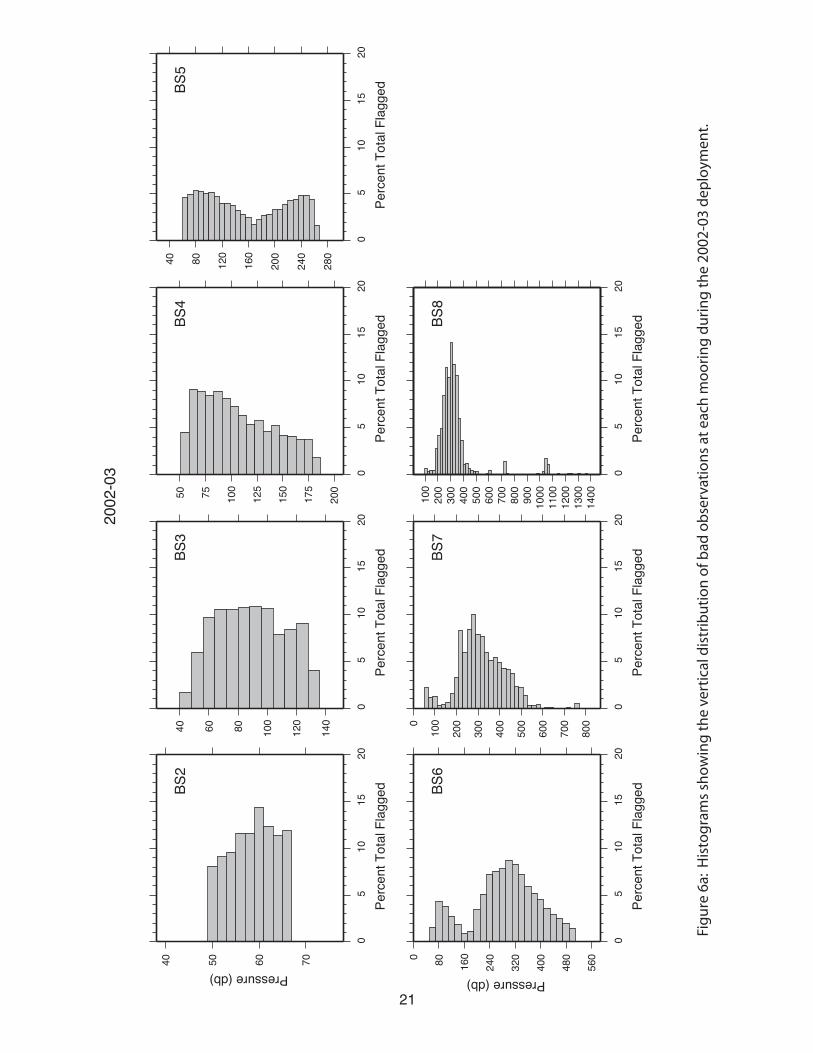
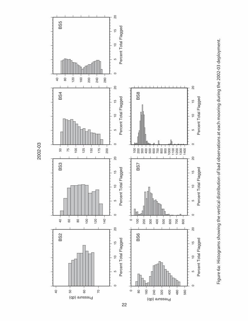
6. (a) Histograms showing the vertical distribution of bad observations (2002-03).
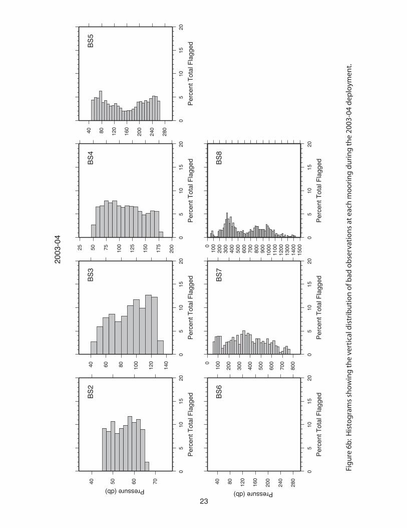
6. (b) Histograms showing the vertical distribution of bad observations (2003-04).
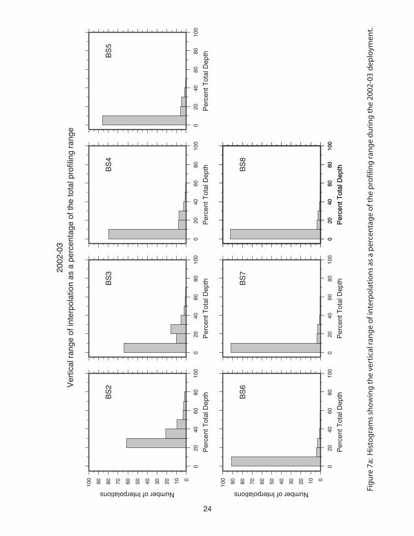
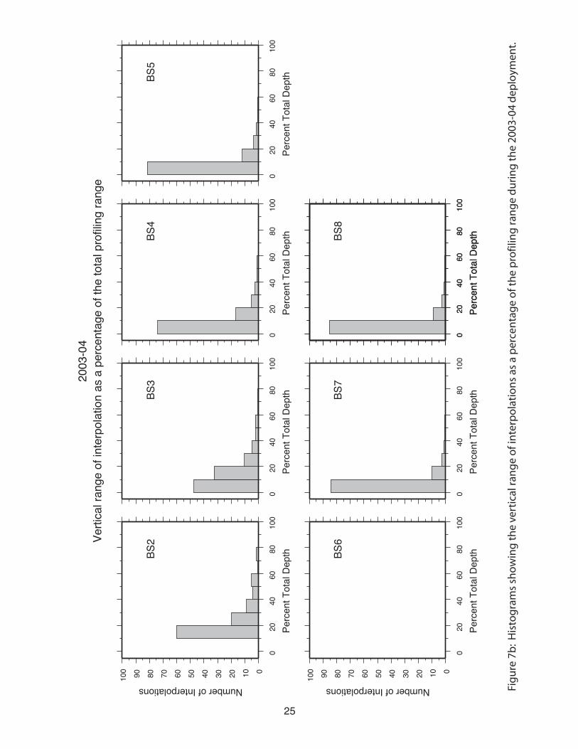
7. (a) Histograms showing the vertical range of interpolated data (2002-03).
7. (b) Histograms showing the vertical range of interpolated data (2003-04).
8. (a) Vertical profiles of raw and interpolated salinity, potential temperature, and
potential density from Aug. 4, 2002 at bs5.
8. (b) Vertical profiles of raw and interpolated salinity, potential temperature, and
potential density from Sep. 30, 2002 at bs4.
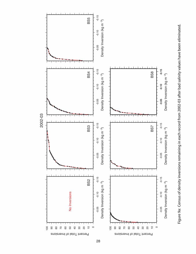
9. (a) Census of density inversions remaining after salinity has been corrected (2002-
03)
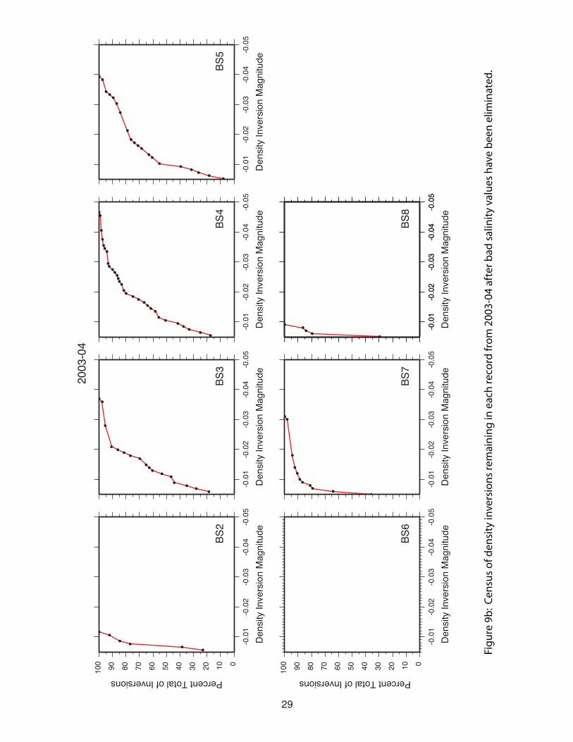
9. (b) Census of density inversions remaining after salinity has been corrected (2003-
04)
1
1. Introduction
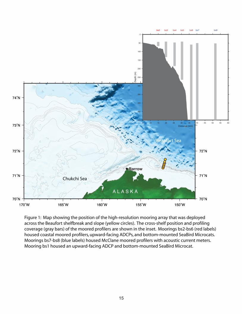
This report describes the collection, calibration, and quality control of moored profiler data from the Beaufort shelf-edge mooring array, a component of the western Arctic Shelf-Basin Interactions (SBI Phase II) experiment. SBI was a multi-year field program, jointly sponsored by the National Science Foundation and Office of Naval Research, designed to investigate the manner in which the continental shelves communicate with the interior Arctic basin. It was motivated by the idea that the effects of global warming will be particularly prominent in the Arctic, resulting in observable changes in the physical and biochemical processes in transition regions like the shelfbreak. An important part of the physical oceanographic component of SBI was a high-resolution moored array deployed across the shelfbreak and upper slope in the Beaufort Sea. The array consisted of eight moorings (bs1-bs8, increasing offshore; Fig. 1). The inner seven moorings (bs1-bs7) were spaced approximately 5 km apart, while the seaward-most mooring (bs8) was located 10 km away. The outer seven moorings (bs2-bs8) each housed a conductivity/temperature/depth (CTD) moored profiler, with coastal moored profilers (CMPs) located at bs2-bs6 and McClane moored profilers (MMPs) at bs7 and bs8. In addition, a fixed Sea-Bird Microcat CTD sensor and upward-facing acoustic Doppler current profiler (ADCP) were included at the bottom of all but the two deepest moorings (bs1-bs6). The moored profilers on the outer two moorings (bs7-bs8) included profiling acoustic current meters (ACMs). The Beaufort mooring array was deployed in August 2002, serviced September 2003, and recovered September 2004. The redundancy of instrumentation on most of the moorings (e.g. profiling and fixed CTDs), and additional ship-based CTD operations, allowed us to perform several levels of quality tests on the moored profiler data. During the servicing operation in 2003 and the recoveries in 2004, the profiling CTDs and the fixed Microcat sensors were calibrated at-sea using intercomparison casts with the ship’s CTD. In addition, by comparing coincident records of temperature and salinity collected by the Microcat and profiling CTDs we have been able to assess the time-dependent behavior of the profiling sensors. The procedures for both are detailed in the sections that follow.
2
2. Moored Profiler Packages
Moored profilers travel up and down a wire-jacketed mooring cable using a battery powered traction drive, carrying sensors that measure temperature, salinity, and velocity on some packages (Doherty et al., 1999; Toole et al., 1999). The result is a time series of repeated high-resolution profiles, having comparable quality to a traditional ship-based CTD station. Each moored profiler in the Beaufort array profiled from a depth of roughly 45 m to approximately 20 m off the bottom (Table 1). The moorings in the Beaufort shelf-edge array contained two varieties of moored profiler (MP): THE MCCLANE MOORED PROFILER (MMP) The two deepest moorings (bs7 - bs8) each housed a McClane Instruments moored profiler (MMP), with a Falmouth Scientific Inc. Excel MCTD (EM-CTD) that measured conductivity, temperature and pressure. The MMP also carries a three-axis acoustic travel-time current meter (ACM) for measuring profiles of velocity (Moorison, et al., 2000). THE COASTAL MOORED PROFILER (CMP) BS2-BS6 each housed a Coastal Moored Profiler (CMP) designed and constructed at the Woods Hole Oceanographic Institution (WHOI). The CMP is a simplified version of the MMP. The chief difference in instrumentation design is that the main electronics and battery are housed inside glass spheres in the CMP instead of a titanium pressure case. Like the MMP, the CMP is equipped with a Falmouth Scientific Inc. EM-CTD. However, unlike the MMP, the CMP does not carry an acoustic current meter.
3. Data Acquisition and Preliminary Processing
The MPs collected profiles of conductivity, temperature, and pressure every six hours at bs2-bs6 (0, 6, 12, 18Z) and twice per day at bs7 and bs8 (0, 6Z), during two consecutive year-long deployments spanning the period August 2002 through September 2004 (Table 1). Overall, the data return was excellent (Table 2). In the first deployment the data return was better than 94% from all of the instruments. During the second deployment, 6 of the 7 moored profilers returned nearly-complete records (better than 90% over most of the instruments). The moored profiler at bs6 flooded during the second deployment, returning no data. After recovering the MP instruments, the binary engineering, EM-CTD and ACM data (MMP only) were extracted from a PC flashcard on the MP controller and converted to ASCII file format. The MP reports engineering data for each profile, including the time (month, year, day, hour, minute, second), motor current (mA), battery voltage (V), pressure (db), and profile speed (dp/dt). The EM-CTD data files include conductivity (mmho), temperature (C), and pressure (db) for each profile. The ACM data files (MMP only) include fields of tilt (deg), normalized compass (x,y,z), and raw path velocities (cm/s).
3
3.1 In-situ Calibration of EM-CTDs Immediately after the MP instruments were recovered, the EM-CTDs and Microcats were mounted to the rosette frame and deployed with the ship’s CTD (Sea-Bird SBE 911+) for an in situ comparison (in deep water). After each cast, the internally recorded data from the mooring’s CTD were downloaded and compared to the ship’s CTD data to determine the amount of drift over the year-long deployment. The key benefit to this at-sea comparison procedure is the ability to assess sensor drift in real-time and avoid the possibility of changing calibrations in transit back to the lab due to time, handling, and/or cleaning.
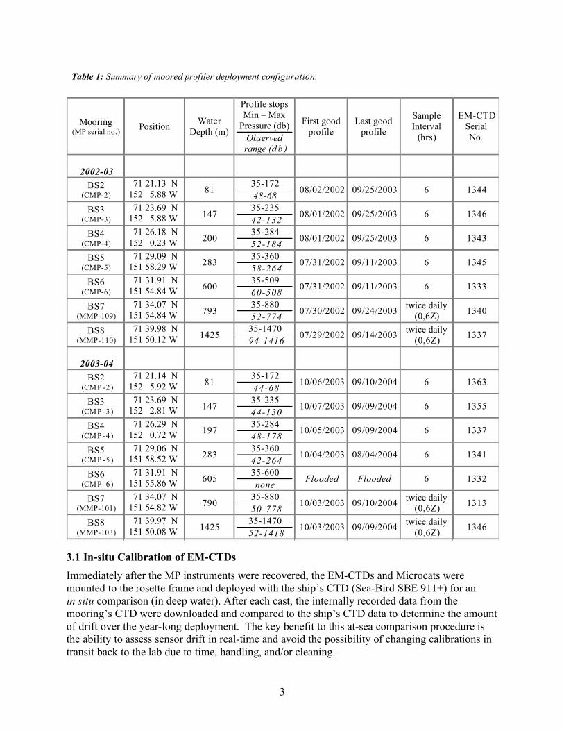
Table 1: Summary of moored profiler deployment configuration.
Mooring (MP serial no.)
Position Water
Depth (m)
Profile stops
Min – Max
Pressure (db)
Observed
range (d b )
First good
profile
Last good
profile
Sample
Interval
(hrs)
EM-CTD
Serial
No.
2002-03
BS2 (CMP-2)
71 21.13 N
152 5.88 W 81
35-172
48-68 08/02/2002 09/25/2003 6 1344
BS3 (CMP-3)
71 23.69 N
152 5.88 W 147
35-235
42-132 08/01/2002 09/25/2003 6 1346
BS4 (CMP-4)
71 26.18 N
152 0.23 W 200
35-284
52-184 08/01/2002 09/25/2003 6 1343
BS5 (CMP-5)
71 29.09 N
151 58.29 W 283
35-360
58-264 07/31/2002 09/11/2003 6 1345
BS6 (CMP-6)
71 31.91 N
151 54.84 W 600
35-509
60-508 07/31/2002 09/11/2003 6 1333
BS7 (MMP-109)
71 34.07 N
151 54.84 W 793
35-880
52-774 07/30/2002 09/24/2003
twice daily
(0,6Z) 1340
BS8 (MMP-110)
71 39.98 N
151 50.12 W 1425
35-1470
94-1416 07/29/2002 09/14/2003
twice daily
(0,6Z) 1337
2003-04
BS2 (CMP-2)
71 21.14 N
152 5.92 W 81
35-172
44-68 10/06/2003 09/10/2004 6 1363
BS3 (CMP-3)
71 23.69 N
152 2.81 W 147
35-235
44-130 10/07/2003 09/09/2004 6 1355
BS4 (CMP-4)
71 26.29 N
152 0.72 W 197
35-284
48-178 10/05/2003 09/09/2004 6 1337
BS5 (CMP-5)
71 29.06 N
151 58.52 W 283
35-360
42-264 10/04/2003 08/04/2004 6 1341
BS6 (CMP-6)
71 31.91 N
151 55.86 W 605
35-600
none Flooded Flooded 6 1332
BS7 (MMP-101)
71 34.07 N
151 54.82 W 790
35-880
50-778 10/03/2003 09/10/2004
twice daily
(0,6Z) 1313
BS8 (MMP-103)
71 39.97 N
151 50.08 W 1425
35-1470
52-1418 10/03/2003 09/09/2004
twice daily
(0,6Z) 1346
4
Table 2: Data return for the moored profilers sorted by deployment. The number of profiles
reflects the total number of profiles with good data over at least one-third of the water column.
The numbers in parentheses represent the percent observed out of the total expected profiles, based on a 6 hourly sampling rate at bs2-bs6 and a twice daily sampling (0, 6 GMT) at bs7 and
bs8 .
Instrument Total Profiles
(Percent of scheduled)
Total Profiles
(Percent of scheduled)
2002-03 2003-04
BS2 1486 (89) 1244 (91)
BS3 1646 (98 ) 839 (62)
BS4 1634 (97 ) 1307 (96)
BS5 1639 (97 ) 1116 (92)
BS6 1621 (100) 0
BS7 811 (96) 682 (100)
BS8 772 (94) 673 (98)
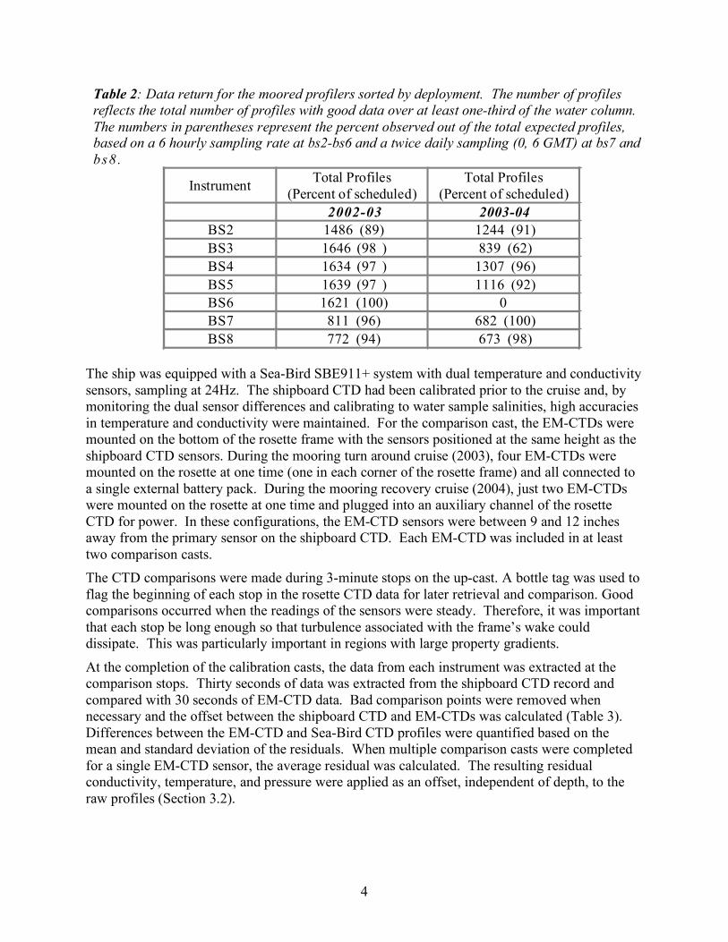
The ship was equipped with a Sea-Bird SBE911+ system with dual temperature and conductivity sensors, sampling at 24Hz. The shipboard CTD had been calibrated prior to the cruise and, by monitoring the dual sensor differences and calibrating to water sample salinities, high accuracies in temperature and conductivity were maintained. For the comparison cast, the EM-CTDs were mounted on the bottom of the rosette frame with the sensors positioned at the same height as the shipboard CTD sensors. During the mooring turn around cruise (2003), four EM-CTDs were mounted on the rosette at one time (one in each corner of the rosette frame) and all connected to a single external battery pack. During the mooring recovery cruise (2004), just two EM-CTDs were mounted on the rosette at one time and plugged into an auxiliary channel of the rosette CTD for power. In these configurations, the EM-CTD sensors were between 9 and 12 inches away from the primary sensor on the shipboard CTD. Each EM-CTD was included in at least two comparison casts. The CTD comparisons were made during 3-minute stops on the up-cast. A bottle tag was used to flag the beginning of each stop in the rosette CTD data for later retrieval and comparison. Good comparisons occurred when the readings of the sensors were steady. Therefore, it was important that each stop be long enough so that turbulence associated with the frame’s wake could dissipate. This was particularly important in regions with large property gradients.
At the completion of the calibration casts, the data from each instrument was extracted at the comparison stops. Thirty seconds of data was extracted from the shipboard CTD record and compared with 30 seconds of EM-CTD data. Bad comparison points were removed when necessary and the offset between the shipboard CTD and EM-CTDs was calculated (Table 3). Differences between the EM-CTD and Sea-Bird CTD profiles were quantified based on the mean and standard deviation of the residuals. When multiple comparison casts were completed for a single EM-CTD sensor, the average residual was calculated. The resulting residual conductivity, temperature, and pressure were applied as an offset, independent of depth, to the raw profiles (Section 3.2).
5
Table 3: Sensor differences from comparison casts between the shipboard (SBE911+) and the EMCTDs recovered
from the moored profilers. Where multiple comparison casts were completed, the value represents an average from
all of the casts. Differences reflect SBE-EMCTD. The final offset that was applied to the EMCTD conductivity
records included an additional 0.002 mS/cm (2002-03) and a 0.001 mS/cm (2003-04) conductivity correction to the
SBE911+ sensor (which itself was calibrated using water sample data collected during the cruise). The post-
recovery casts at bs5 (2003-04) could not be used due to bad pressure values and no calibration cast was done for
bs6 (2003-04) because the EMCTD flooded during the deployment. (* This comparison was done after the EMCTD
sensor was cleaned. The pre-cleaned comparison cast was not successful).
Mooring (EMCTD serial no.)
Pressure (db) Temperature (C) Conductivity
(mS/cm)
Conductivity
Offset
Applied
2002-03 +0.002 mS/cm
BS2 (1344)
0.34 0.006 0.047 0.049
BS3 (1346)
-0.66 0.005 0.011 0.013
BS4 (1343)
-0.28 0.002 -0.008 -0.006
BS5 (1345)
-2.21 0.005 -0.002 0
BS6 (1333)
-0.63* 0.006* -0.011* -0.009
BS7 (1340)
flood flood flood 0
BS8 (1337)
-1.37 0.003 -0.008 -0.006
Average
(absolute difference) 0.915 0.005 0.015 0.014
2003-04 +0.001 mS/cm
BS2 (1363)
-0.98 -0.0006 -0.013 -0.012
BS3 (1355)
0.25 -0.0029 0.016 0.017
BS4 (1337)
-0.32 0.0029 -0.008 -0.007
BS5 (1341)
--- --- --- ---
BS6 (1332)
--- --- --- ---
BS7 (1313)
-0.4 0.009 -0.105 -0.104
BS8 (1346)
-0.37 0.004 -0.005 -0.004
Average
(absolute difference) 0.464 0.004 0.030 0.029

6
On average, the EM-CTD temperature differed by 0.004-0.005 °C compared with the shipboard CTD and the conductivity differed by 0.015-0.03 mS/cm (Table 3). Multiple comparison casts showed that the EM-CTD temperature sensors had reproducible results within 0.0015 °C (individual casts not shown in Table 3). By comparison, depending on the particular CTD, conductivity shifted between 0.002 - 0.008 mS/cm (0.003-0.009 psu) between casts. Therefore, we estimate that the salinity data from the moored profilers have an accuracy of better than 0.009 while the temperature data have an accuracy of 0.002 ºC, close to the factory specified accuracy of the sensor. 3.2 Creation of Gridded Data Product Once the data was downloaded from the flashcards of the MP instruments and unpacked, we used the processing system developed by John Toole at the Woods Hole Oceanographic Institution to process the raw sensor data and output pressure gridded profiles of the data from the CTD (and ACM where applicable). This was completed using a suite of Matlab scripts that perform three tasks: (1) Merge the raw data files and store all variables in one Matlab-formatted file for each profile, (2) create and examine a summary of the data, and (3) average the CTD (and ACM) data into user specified pressure bins. Before each CTD (ACM) profile was bin-averaged onto a standard pressure grid, the data was checked to insure that all variables fall within sensible ranges. Data falling outside sensible ranges were interpolated (nominally -3-10 ºC for temperature, 10-60 mS/cm for conductivity, and outside the pressure stops specified for each mooring). Next, we applied the sensor calibration data for pressure, temperature and conductivity determined from the comparison casts described above. Finally, the edited and calibrated data was bin-averaged with respect to specified pressure levels (2db bin widths) and derived quantities were calculated (salinity, potential temperature, and potential density). NaN values are used as place-holders in cells with no data. A gridded file was output for each profile with the following variables (filename, grd####.mat, where #### is the profile number):
startdaytime start day and time of the profile (encoded with DATENUM, see below) stopdaytime stop day and time of the profile (encoded with DATENUM, see below) pgrid center values of the pressure grid used in the bin-average (db) ctimave day and time of values averaged in each pgrid bin (see below) pave average of the pressure values in each pgrid bin (db) tave bin-averaged temperature (°C) s_ave bin-averaged salinity computed from pave, tave, and cave thetave potential temperature computed from pave, tave, and s_ave (°C) sigthave potential density computed rom pave, tave, and s_ave (kg m-3) cave bin-averaged conductivity (mmho) dpdtave average time rate of change of pressure (db/sec) cscan1(2) indices of the CTD data averaged in each pgrid bin For the MMPs, the following variables are also included: uave average east velocity in each pgrid bin (cm/s) vave average north velocity in each pgrid bin (cm/s)
7
wave average relative vertical velocity in each pgrid bin (cm/s) ascan1(2) indices of the ACM data averaged in each pgrid bin
4. Post Cruise Calibration of Conductivity
The in situ comparison casts between the shipboard Sea-Bird CTD and the EM-CTDs were valuable and provided a single calibration point that was applied as an offset to the temperature, salinity, and pressure records from each MP. However, even though extreme care was taken to avoid touching or otherwise “cleaning” the conductivity cells on the EM-CTDs prior to the comparison casts, it is likely that the physical recovery of the moorings probably resulted in some flushing of the sensors, perhaps artificially improving the sensor comparison. Fortunately, BS2-BS6 also housed a Sea-Bird Microcat CTD that was mounted near the bottom of the mooring (out of the euphotic zone) and collected hourly observations of temperature and conductivity during the two consecutive deployments. These data provide a means to assess the true in situ, time-dependent behavior of the profiling CTDs at these sites.
While the temperature and pressure sensors on the Falmouth Scientific, Inc. EM-CTD are relatively stable, the conductivity sensor is vulnerable to a number of external influences that can adversely affect the accuracy of the sensor. Both the measured resistance and the geometry of the sampled water are equally important in the determination of conductivity. For this reason, in order to obtain stable sensor readings throughout its deployment, the cell must hold its dimensions despite the effect of corrosion, mineral depositions, and marine growth.
The Falmouth Scientific EM-CTD is an inductive sensor, meaning that a transformer is used to couple a known voltage to the water and the resulting current flow is detected using a second transformer core. A defining feature of all inductive sensors is that they have fields external to the sensor’s cell volume. In other words, the electrical current flows in closed paths through the space between the transformer cores so that some of the resistance occurs outside the relatively well-defined geometry of the hole itself. The calibration of an inductive sensor may be shifted if nearby objects such as guards, struts, sensor housings, or marine growth distort this external field, thereby affecting the geometry of the cell. Because the EM-CTD is sensitive enough to resolve a change in resistivity of the volume of water within a 3 inch radius around the cell, it is difficult to protect from the effect of biological fouling, shedding of insulating paint or coatings, or corroding of conductive surfaces on the stem, guard cage, base plate and mounting housing of the conductivity cell. Of these, biofouling on the conductivity cell is one of the predominant causes of sensor drift, resulting in higher measured resistance by the sensor and hence lower conductivity readings. The effect is reflected in a relatively slow drift toward lower conductivity (salinity) over the course of a deployment. By contrast, sudden jumps in conductivity and high-frequency sensor noise may result from contact with biological matter such as seaweed (e.g. Doherty et al., 1999). 4.1 Microcat Comparisons Due to the sensor design and its physical location near the bottom of the mooring, we assume that the conductivity measured by the Sea-Bird Microcat CTD will be more stable over time than that measured by the profiling EM-CTD (which spent part of each day sampling the upper part of the water column.) The Microcat contains an electrode conductivity cell with a fully internal field, unlike the inductive sensor on the EM-CTD. Because its field is internal, small amounts of

8
antifoul material can be placed at the ends of the cell, effectively preventing fouling and reducing sensor drift. In the Beaufort array, the Microcat sensors were mounted on the mooring near the bottom away from regions with higher biological activity, further reducing the chances for bio-fouling and sensor drift. Hence, we use the conductivity recorded by the Microcat at each mooring to compute a time-dependent calibration coefficient that can be used to adjust the EM-CTD conductivity record.
Like the EM-CTDs, the Microcats were calibrated at-sea using intercomparison casts with the ship’s CTD. The calibrated Microcat time series of conductivity was then compared with the deepest observations of conductivity recorded by the MP on the same mooring. The procedure involved the following steps:
1. Interpolate the hourly Microcat data to align with the 6-hourly MP time series. 2. Extract data from the deepest bin in the MP profiles.
3. Calculate the time-dependent conductivity ratio, defined as:
!
r(t) =cMicrocat
(t)
cEMCTD
(t),
where
!
cMicrocat
is the conductivity measured by the Microcat near the bottom, and
!
cEMCTD
is the conductivity measured by the MP at its deepest bin.
4. Spikes in the conductivity ratio can result from differences in sensor response times. It is necessary to smooth over the spikes so that they do not contaminate the final calibration of the EM-CTD data. We smoothed the spikes by performing an iterative polynomial fit to
!
r(t). The iterative process involves fitting a 2nd order polynomial to
!
r(t), computing the residual between the fit and the actual ratio, excluding values of
!
r(t) that are greater than twice the standard deviation of the residuals, and calculating a new polynomial fit to the edited time series of
!
r(t).
5. The Microcat and the deepest bin of the EM-CTD were not collocated, but were separated between 4 and 15 m (Table 4). If the water column is stratified over these vertical scales, the conductivity ratio,
!
r(t), will reflect these differences rather than just sensor error. In order to ensure that
!
r(t) was dominated by sensor differences, we estimated the vertical gradients in conductivity over the deepest portion of the EM-CTD profiling range, choosing a vertical distance comparable to the separation between the EM-CTD and Microcat. An iterative fit was used to smooth the resulting time series of vertical differences, similar to the one applied to
!
r(t). Finally, the time series of vertical differences,
!
"cz, was compared to a smoothed version of the differences between the
instruments,
!
cEMCTD
(t)" (r(t) #1) . If the curves were similar, then some of the difference between the conductivity measured by the Microcat and the EM-CTD was deemed to be from physical processes, not necessarily sensor drift. If this is the case,
!
cEMCTD
would need to be adjusted by
!
"cz, before comparing to
!
cMicrocat
and calculating
!
r(t).
6. In at least one case, a piecewise linear fit was applied to r(t) instead of a polynomial fit. In this case, gradual changes in
!
r(t) were interrupted by periods of abrupt change making a polynomial fit inappropriate. Each linear fit was iterative in nature, requiring that the

9
difference between the fit to r(t) and r(t) be less than twice the standard deviation of the residual time series (as in step 5).
7. Once the sensor comparison was complete and the calibration ratio was determined using one of the methods in steps 4-6, the final calibrated conductivity was determined by
!
ccalibrated
(z,t) = cemctd
(z,t) " r(t). In the calibration, the ratio was applied to each profile of conductivity, independent of depth. Finally, new salinity values were calculated from the time series of calibrated conductivity.
8. Shipboard CTD stations were occupied near each of the moorings upon deployment and recovery. As a final (independent) check, the profiles from these CTD stations were compared with the closest MP profile (in time) to ensure that there were no significant differences introduced by our calibration.
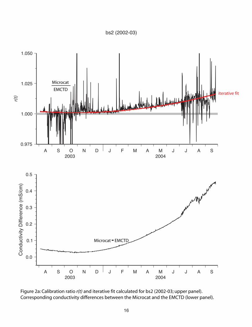
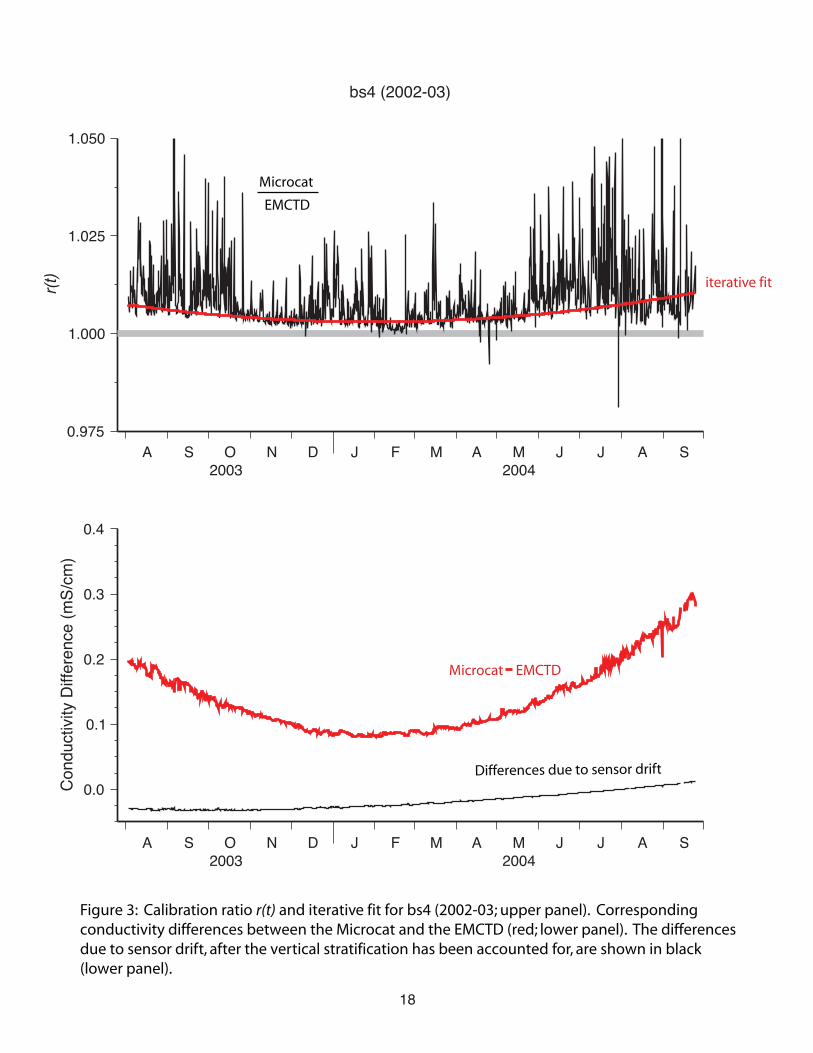
4.2 Calibration results The results from the Microcat/EM-CTD comparisons are summarized in Table 4. We determined that vertical property gradients were insignificant at a majority of the moorings so that a simple polynomial fit (step 4) could be used to describe the shape of r(t). As an example, the sensor comparison from bs2 (2002-03) exhibits the expected drift toward lower salinities as a result of bio-fouling (Figure 2a). Vertical gradients did however dominate the sensor comparison in three instances – at bs4 during both deployments and at bs5 during the 2003-04 deployment (Table 4). Figure 3 shows an example from bs4 (2002-03). In this case, the difference in conductivity measured by the sensors has a parabolic shape in time. However, after the vertical gradients have been estimated and removed as outlined in step 5 the differences are monotonic as we would expect if one sensor were drifting relative to the other.
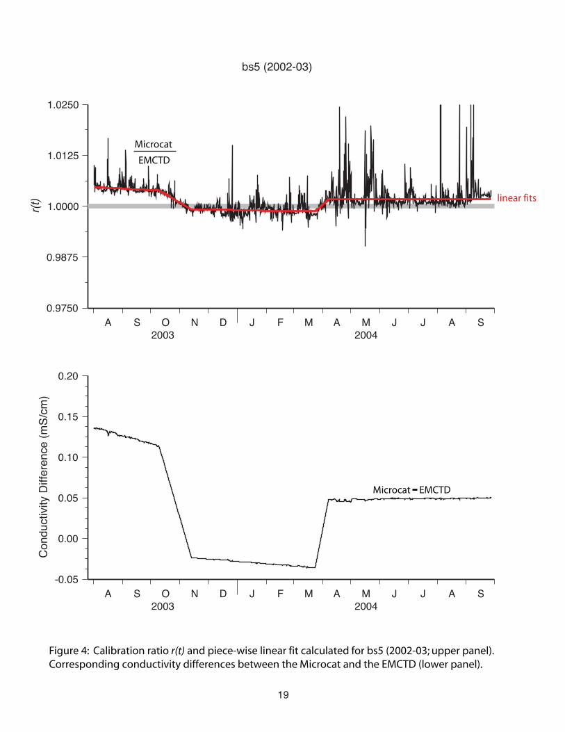
As mentioned previously, there was one case where the shape of r(t) did not lend itself to a simple polynomial fit and a piece-wise linear fit was applied instead (bs5, 2002-03). In this case, the calibration ratio exhibited periods of gradual change that were interrupted by abrupt shifts to larger or smaller values (Figure 4). It is not clear what caused this sensor behavior, however it is possible that accumulated growth was suddenly flushed or knocked from the sensor, causing the conductivity to rebound partway through the deployment. Then again, this does not appear to be the entire story, particularly since the jumps in r(t) are not monotonic. We found a problem with just one calibration when we compared the calibrated time series with pre- and post- deployment shipboard hydrography (bs6, 2002-03). It was determined that the Microcat at bs6 had a bad pressure sensor that probably contributed to the problem. In the end, a linear drift was derived from comparison of the EMCTD to the shipboard CTD stations only and applied to the EM-CTD data at this site. The offsets at the beginning and end of the deployment were calculated as the average conductivity difference between the EM-CTD and the nearest shipboard cast over a depth range of 400-500m. This depth range corresponds to the part of the water column where record-long conductivity variations were minimized.
At BS7-BS8, where there were no Microcats to use for comparison, the hydrographic station data collected near the moorings during the deployment and recovery cruises were used to check for sensor drift. The residuals at these sites were small with no indication of drift. Therefore, no additional offset was applied at these moorings.
10
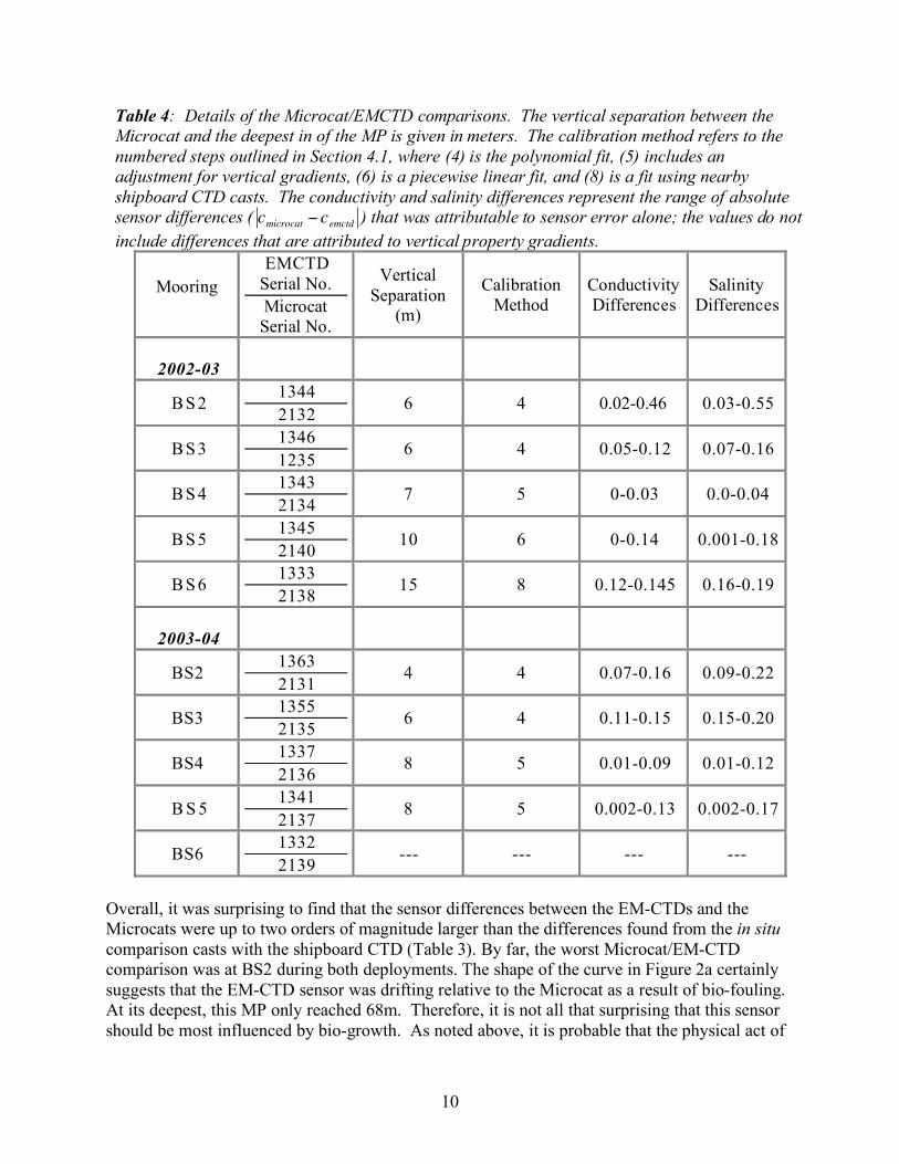
Table 4: Details of the Microcat/EMCTD comparisons. The vertical separation between the
Microcat and the deepest in of the MP is given in meters. The calibration method refers to the
numbered steps outlined in Section 4.1, where (4) is the polynomial fit, (5) includes an
adjustment for vertical gradients, (6) is a piecewise linear fit, and (8) is a fit using nearby
shipboard CTD casts. The conductivity and salinity differences represent the range of absolute
sensor differences (
!
cmicrocat
" cemctd
) that was attributable to sensor error alone; the values do not
include differences that are attributed to vertical property gradients.
Mooring
EMCTD
Serial No.
Microcat
Serial No.
Vertical
Separation (m)
Calibration
Method
Conductivity
Differences
Salinity
Differences
2002-03
B S 2 1344
2132 6 4 0.02-0.46 0.03-0.55
B S 3 1346
1235 6 4 0.05-0.12 0.07-0.16
B S 4 1343
2134 7 5 0-0.03 0.0-0.04
B S 5 1345
2140 10 6 0-0.14 0.001-0.18
B S 6 1333
2138 15 8 0.12-0.145 0.16-0.19
2003-04
BS2 1363
2131 4 4 0.07-0.16 0.09-0.22
BS3 1355
2135 6 4 0.11-0.15 0.15-0.20
BS4 1337
2136 8 5 0.01-0.09 0.01-0.12
B S 5 1341
2137 8 5 0.002-0.13 0.002-0.17
BS6 1332
2139 --- --- --- ---
Overall, it was surprising to find that the sensor differences between the EM-CTDs and the Microcats were up to two orders of magnitude larger than the differences found from the in situ comparison casts with the shipboard CTD (Table 3). By far, the worst Microcat/EM-CTD comparison was at BS2 during both deployments. The shape of the curve in Figure 2a certainly suggests that the EM-CTD sensor was drifting relative to the Microcat as a result of bio-fouling. At its deepest, this MP only reached 68m. Therefore, it is not all that surprising that this sensor should be most influenced by bio-growth. As noted above, it is probable that the physical act of

11
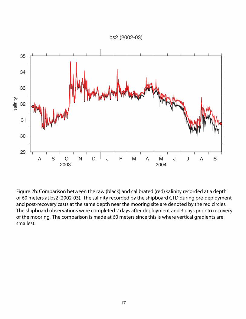
recovering the moorings resulted in some flushing of the sensors – hence the reason this Microcat comparison was undertaken in the first place. In fact, the original comparison cast at BS2 had an offset of 0.05 mS/cm relative to the SBE911+ conductivity (Table 3). However, in a second comparison cast, immediately after it had been cleaned, the sensor difference was reduced by an order of magnitude to 0.005 mS/cm. Hence, it is not unlikely that a large quantity of growth on the sensor (0.46 mS/cm worth; Table 4) was partially washed off during recovery (leaving 0.05 mS/cm; Table 3). After it was finally cleaned, the sensor differences were reduced even further to an acceptable 0.005 mS/cm. Indeed, the final comparison between the calibrated EM-CTD record and nearby shipboard CTD stations indicates that the correction applied for the relatively large offset observed between the Microcat and EM-CTD is accurate (Figure 2b).
In general, using the Microcats to adjust the EM-CTD conductivity records improved the sensor agreement by a factor of 10 or more. A comparison between deployment-long average density sections constructed from the raw and calibrated MP data showed that the calibrated density field is more physically meaningful and agrees better with shipboard hydrography than the raw fields. Comparing the Microcat data with the EM-CTD observations proved to be more valuable than the calibration casts done with the shipboard CTD. However, this calibration procedure would have been greatly simplified if the Microcats had been mounted closer to the bottom stop of the MP on the mooring (e.g. 1-2 meters). We would recommend that this be taken into account in future mooring designs.
5. Data Quality Control
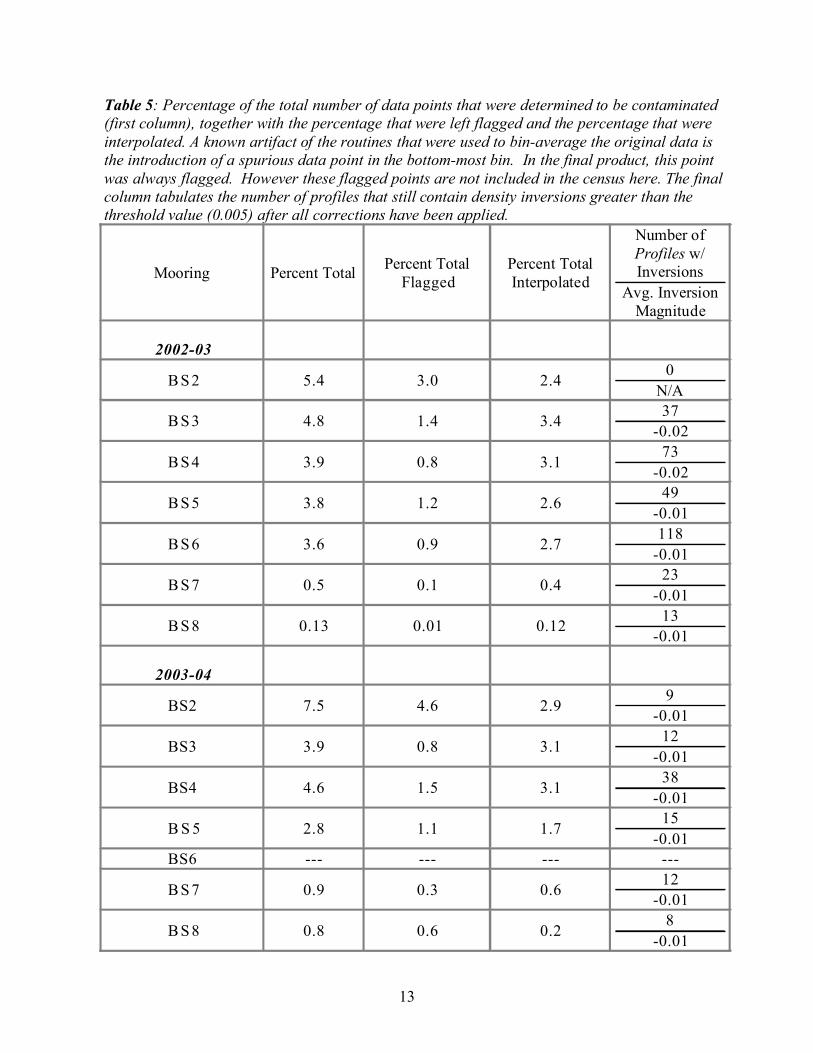
Despite the editing and averaging performed in the initial data processing (Section 3.2), some spurious salinity points still needed to be filtered from the dataset. The conductivity record from the EM-CTD occasionally exhibits short periods of highly anomalous values. Because the cell recovers quickly, it is probable that the anomalous readings are caused when seaweed or some other material covers the cell (this is in contrast to the longer period drifts that are most often caused by something growing on the cell). Fortunately, the problem is less prevalent in the Arctic than at lower latitudes, particularly during periods when the sea surface is ice covered. Spurious salinity values were identified by examining profiles of potential density – the idea being that spurious values will cause significant density inversions. Potential density profiles were computed from the calibrated temperature and salinity data and searched for inversions exceeding -0.005 kg/m3 (our estimate of the sensitivity of the EM-CTD sensors derived from the in situ comparison casts discussed in Section 3.1). Each of the profiles containing inversions was then manually examined and, when possible, the questionable data were replaced by vertical interpolation. The neighboring five profiles in time were also examined to be sure that temporal continuity was maintained in the interpolated data. In the remaining cases the bad data was flagged NaN. A census of the bad data that were identified is presented in Table 5.
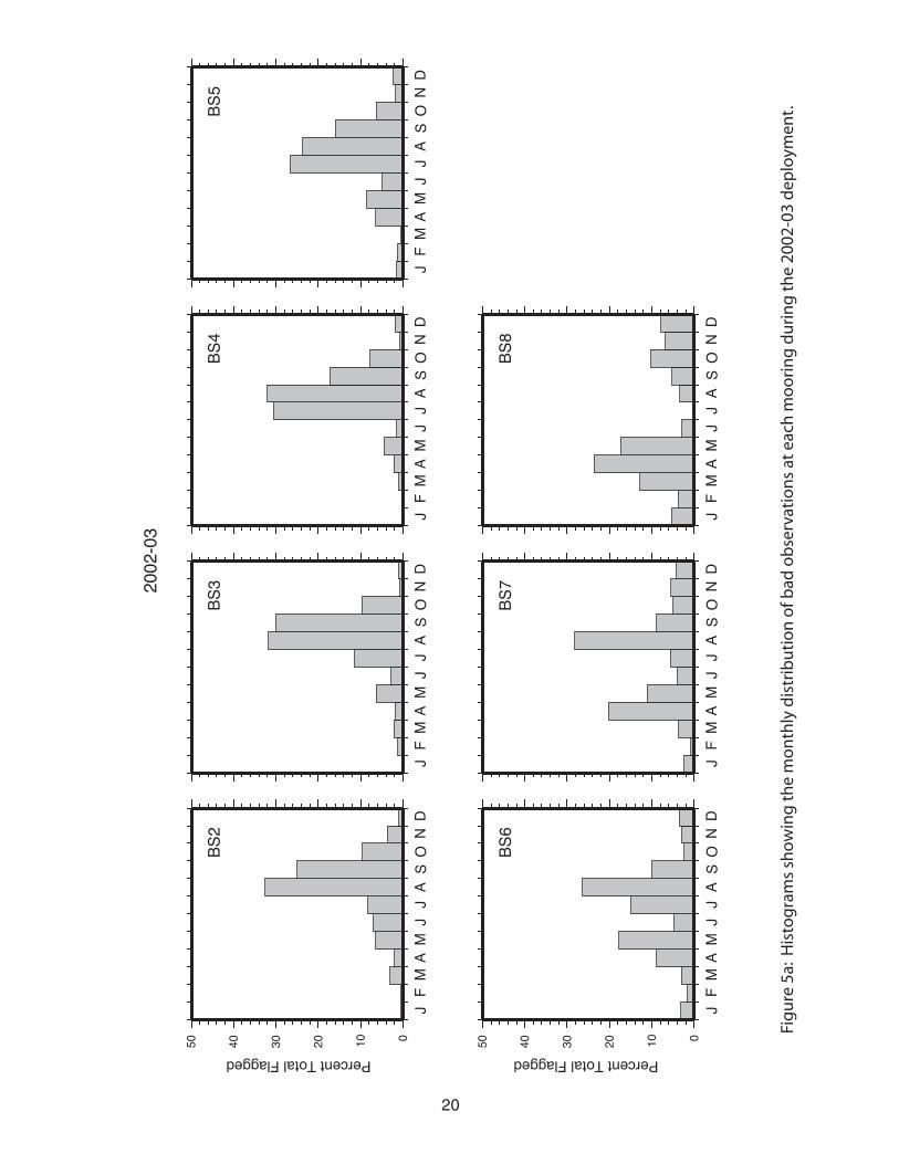
Histograms illustrate the distribution of contaminated data in Figures 5-7. During 2002-03, the majority of the flagged data was clustered in summer (Aug.-Sep.), with a secondary peak during winter (Feb.-Apr.) at the seaward moorings (Figure 5a). By contrast, during 2003-04 the histograms show a dual peak, with bad data clustered in fall (Oct.-Nov.) and early summer (Jun.-Jul.) at all of the moorings (Figure 5b). The vertical distribution of contaminated data is shown in Figure 6 and the patterns are similar during both deployments. The most notable feature is the

12
peak near 300 db at the deeper moorings (bs6-bs8). The peak is particularly pronounced at bs8 during 2002-03 (Figure 6a).
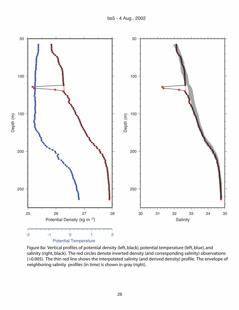
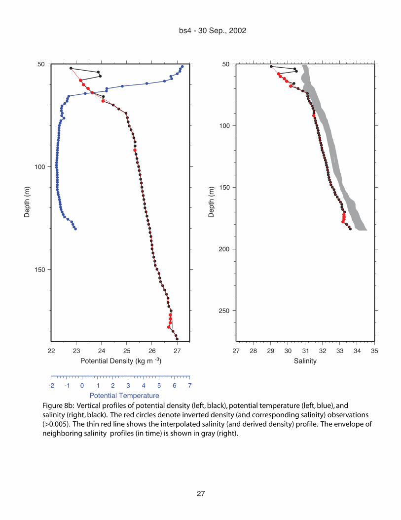
While spurious observations were identified using profiles of potential density, the interpolation was performed on just the salinity profiles since the conductivity sensor tends to be most susceptible to spikes (experience suggests that the temperature and pressure sensors on the EM-CTD are much more stable). An interpolation was not attempted if it was determined that a large portion of the profile was contaminated – in these cases the bad salinity values were flagged. With the exception of bs2, we were able to interpolate the majority of the questionable points (Table 5). BS2 was deployed in such shallow water (80m) that when contamination occurred it occupied a larger fraction of the total profiling range. On average, interpolations typically spanned 8 m (4 MP bins), an average of only 4-6% of the total profiling range of the instruments (Figure 7). An example of a profile before and after interpolation is presented in Figures 8a & 8b. Overall, less than 1% of the profiles collected during both deployments were entirely flagged (and dropped) due to bad data.
After the profiles were either corrected or flagged, the edited time series was scanned a second time for inversions. Even after “fixing” the problem profiles, inversions occasionally remained (although the magnitude of the remaining inversions was always greatly reduced). Most often, the remaining inversions were associated with warm, salty water underlying cool, fresh water. In all cases, the temperature maximum occupied several depth bins (6-8 m) and did not appear suspicious. As a result these data were unaltered. In the end, we were able to eliminate virtually all density inversions with magnitudes exceeding -0.05 kg/m3, leaving more than 99% of the data free of inversions (Figure 9; Table 5).
13
Table 5: Percentage of the total number of data points that were determined to be contaminated
(first column), together with the percentage that were left flagged and the percentage that were
interpolated. A known artifact of the routines that were used to bin-average the original data is
the introduction of a spurious data point in the bottom-most bin. In the final product, this point
was always flagged. However these flagged points are not included in the census here. The final
column tabulates the number of profiles that still contain density inversions greater than the
threshold value (0.005) after all corrections have been applied.
Mooring Percent Total Percent Total
Flagged
Percent Total
Interpolated
Number of
Profiles w/
Inversions
Avg. Inversion
Magnitude
2002-03
B S 2 5.4 3.0 2.4 0
N/A
B S 3 4.8 1.4 3.4 37
-0.02
B S 4 3.9 0.8 3.1 73
-0.02
B S 5 3.8 1.2 2.6 49
-0.01
B S 6 3.6 0.9 2.7 118
-0.01
B S 7 0.5 0.1 0.4 23
-0.01
B S 8 0.13 0.01 0.12 13
-0.01
2003-04
BS2 7.5 4.6 2.9 9
-0.01
BS3 3.9 0.8 3.1 12
-0.01
BS4 4.6 1.5 3.1 38
-0.01
B S 5 2.8 1.1 1.7 15
-0.01
BS6 --- --- --- ---
B S 7 0.9 0.3 0.6 12
-0.01
B S 8 0.8 0.6 0.2 8
-0.01

14
6. Final Products
The final processed data are stored in matlab-formatted files. Each file (bsXX_YY.mat) contains the full set of moored profiler data for instrument XX during deployment year 20YY. The CTD data have been calibrated, de-spiked, and bad data points have been either corrected or replaced with NaN values as described in this report. The files contain a single structure function with the following variables (each row in an array corresponds with a single profile completed by the moored profiler): MP.time day and time of values averaged in each pgrid bin MP.pgrid center values of the pressure grid used in the bin-average (db) MP.pave average of the pressure values in each pgrid bin (db) MP.tave bin-averaged temperature (°C) MP.cave bin-averaged conductivity (mmho) MP.s_ave bin-averaged salinity (psu) computed from MP.pave, MP.tave, and MP.cave The two moorings deployed farthest offshore (bs7 and bs8) included acoustic current meters. These files contain the following additional variables: MP.uave bin-averaged east velocity in each pgrid bin (cm/s) MP.vave bin-averaged north velocity in each pgrid bin (cm/s) MP.wave bin-averaged relative vertical velocity in each pgrid bin (cm/s) The time vectors represent serial time from January 1, 0000 (encoded date using the matlab function DATNUM). Acknowledgements Funds for the collection and processing of this data were provided by the Office of Naval Research under grant N00014-02-1-0317. We are grateful to J. Toole for his valuable input on the setup and deployment of the moored profilers, and on the processing of their data. References Doherty, K. W., D. E. Frye, S. P. Liberatore, and J. M. Toole, 1999. A moored profiling instrument. Journal of Atmospheric and Oceanic Technology, 16, 1816-1829. Morrison, A. T., J. D. Billings, K. W. Doherty, and J. M. Toole, 2000. The McLane Moored Profiler: A platform for physical, biological, and chemical oceanographic measurements. Proceedings of OCEANS 2000, MTS/IEE/OES, Vol. I, 353-358. Toole, J. M., K. W. Doherty, D. E. Frye, and S. P. Liberatore, 1999. Velocity measurements from a moored profiling instrument. Proceedings of IEEE, Sixth Working Conference on Current Measurement, March 11-13, 1999, San Diego, pp. 144-149.
170˚W 165˚W 160˚W 155˚W 150˚W70˚N 70˚N
71˚N 71˚N
72˚N 72˚N
73˚N
74˚N
170˚W 165˚W 160˚W 155˚W 150˚W70˚N 70˚N
71˚N 71˚N
72˚N 72˚N
73˚N
74˚N
A L A S K A
Barrow
Figure 1: Map showing the position of the high-resolution mooring array that was deployed across the Beaufort shelfbreak and slope (yellow circles). The cross-shelf position and profiling coverage (gray bars) of the moored profilers are shown in the inset. Moorings bs2-bs6 (red labels)housed coastal moored profilers, upward-facing ADCPs, and bottom-mounted SeaBird Microcats. Moorings bs7-bs8 (blue labels) housed McClane moored profilers with acoustic current meters. Mooring bs1 housed an upward-facing ADCP and bottom-mounted SeaBird Microcat.
Beaufort Sea
Chukchi Sea
0
50
100
150
200
250
300
350
400
450
500
Dep
th (m
)
5 10 15 20 25 30 35 40 45 50 55 60
Distance (km)
bs2 bs3 bs4 bs5 bs6 bs7 bs8
15
0.975
1.000
1.025
1.050
r(t)
A S O N D J F M A M J J A S2003 2004
bs2 (2002-03)
0.0
0.1
0.2
0.3
0.4
0.5
Con
duct
ivity
Diff
eren
ce (m
S/cm
)
A S O N D J F M A M J J A S2003 2004
Microcat EMCTD
iterative fit
Microcat
EMCTD
Figure 2a: Calibration ratio r(t) and iterative fit calculated for bs2 (2002-03; upper panel). Corresponding conductivity differences between the Microcat and the EMCTD (lower panel).
16
29
30
31
32
33
34
35
salin
ity
A S O N D J F M A M J J A S2003 2004
bs2 (2002-03)
Figure 2b: Comparison between the raw (black) and calibrated (red) salinity recorded at a depth of 60 meters at bs2 (2002-03). The salinity recorded by the shipboard CTD during pre-deployment and post-recovery casts at the same depth near the mooring site are denoted by the red circles.The shipboard observations were completed 2 days after deployment and 3 days prior to recovery of the mooring. The comparison is made at 60 meters since this is where vertical gradients are smallest.
17
0.975
1.000
1.025
1.050
r(t)
A S O N D J F M A M J J A S2003 2004
bs4 (2002-03)
0.0
0.1
0.2
0.3
0.4
Con
duct
ivity
Diff
eren
ce (m
S/cm
)
A S O N D J F M A M J J A S2003 2004
Microcat EMCTD
Differences due to sensor drift
iterative fit
Microcat
EMCTD
Figure 3: Calibration ratio r(t) and iterative fit for bs4 (2002-03; upper panel). Correspondingconductivity differences between the Microcat and the EMCTD (red; lower panel). The differencesdue to sensor drift, after the vertical stratification has been accounted for, are shown in black (lower panel).
18
0.9750
0.9875
1.0000
1.0125
1.0250
r(t)
A S O N D J F M A M J J A S2003 2004
bs5 (2002-03)
-0.05
0.00
0.05
0.10
0.15
0.20
Con
duct
ivity
Diff
eren
ce (m
S/cm
)
A S O N D J F M A M J J A S2003 2004
Microcat EMCTD
linear fits
Microcat
EMCTD
Figure 4: Calibration ratio r(t) and piece-wise linear fit calculated for bs5 (2002-03; upper panel). Corresponding conductivity differences between the Microcat and the EMCTD (lower panel).
19
2002
-03
BS2
JF
MA
MJ
JA
SO
ND
JF
MA
MJ
JA
SO
ND
BS3
JF
MA
MJ
JA
SO
ND
BS4
JF
MA
MJ
JA
SO
ND
BS5
JF
MA
MJ
JA
SO
ND
BS6
BS7
JF
MA
MJ
JA
SO
ND
BS8
JF
MA
MJ
JA
SO
ND
Percent Total Flagged Percent Total Flagged
01020304050 01020304050
Fig
ure
5a:
His
tog
ram
s sh
ow
ing
th
e m
on
thly
dis
trib
uti
on
of b
ad o
bse
rvat
ion
s at
eac
h m
oo
rin
g d
uri
ng
th
e 20
02-0
3 d
eplo
ymen
t.
20
40 50 60 70
Pressure (db)
05
1015
20
Perc
ent T
otal
Fla
gged
2002
-03
BS2
40 60 80 100
120
140
05
1015
20
Perc
ent T
otal
Fla
ggedBS
350 75 10
0
125
150
175
200
05
1015
20
Perc
ent T
otal
Fla
ggedBS
440 80 12
0
160
200
240
280
05
1015
20
Perc
ent T
otal
Fla
ggedBS
5
0 80 160
240
320
400
480
560
Pressure (db)
05
1015
20
Perc
ent T
otal
Fla
ggedBS
6
0
100
200
300
400
500
600
700
800
05
1015
20
Perc
ent T
otal
Fla
ggedBS
710
020
030
040
050
060
070
080
090
010
0011
0012
0013
0014
00
05
1015
20
Perc
ent T
otal
Fla
ggedBS
8
Fig
ure
6a:
His
tog
ram
s sh
ow
ing
th
e ve
rtic
al d
istr
ibu
tio
n o
f bad
ob
serv
atio
ns
at e
ach
mo
ori
ng
du
rin
g t
he
2002
-03
dep
loym
ent.
21
40 50 60 70
Pressure (db)
05
1015
20
Perc
ent T
otal
Fla
gged
2002
-03
BS2
40 60 80 100
120
140
05
1015
20
Perc
ent T
otal
Fla
ggedBS
350 75 10
0
125
150
175
200
05
1015
20
Perc
ent T
otal
Fla
ggedBS
440 80 12
0
160
200
240
280
05
1015
20
Perc
ent T
otal
Fla
ggedBS
5
0 80 160
240
320
400
480
560
Pressure (db)
05
1015
20
Perc
ent T
otal
Fla
ggedBS
6
0
100
200
300
400
500
600
700
800
05
1015
20
Perc
ent T
otal
Fla
ggedBS
710
020
030
040
050
060
070
080
090
010
0011
0012
0013
0014
00
05
1015
20
Perc
ent T
otal
Fla
ggedBS
8
Fig
ure
6a:
His
tog
ram
s sh
ow
ing
th
e ve
rtic
al d
istr
ibu
tio
n o
f bad
ob
serv
atio
ns
at e
ach
mo
ori
ng
du
rin
g t
he
2002
-03
dep
loym
ent.
22
40 50 60 70
Pressure (db)
05
1015
20
Perc
ent T
otal
Fla
gged
2003
-04
BS2
40 60 80 100
120
140
05
1015
20
Perc
ent T
otal
Fla
ggedBS
325 50 75 10
0
125
150
175
200
05
1015
20
Perc
ent T
otal
Fla
ggedBS
440 80 12
0
160
200
240
280
05
1015
20
Perc
ent T
otal
Fla
ggedBS
5
BS6
40 80 120
160
200
240
280
Pressure (db)
05
1015
20
Perc
ent T
otal
Fla
gged
0
100
200
300
400
500
600
700
800
05
1015
20
Perc
ent T
otal
Fla
ggedBS
7
010
020
030
040
050
060
070
080
090
010
0011
0012
0013
0014
0015
00
05
1015
20
Perc
ent T
otal
Fla
ggedBS
8
Fig
ure
6b
: H
isto
gra
ms
sho
win
g t
he
vert
ical
dis
trib
uti
on
of b
ad o
bse
rvat
ion
s at
eac
h m
oo
rin
g d
uri
ng
th
e 20
03-0
4 d
eplo
ymen
t.
23
0102030405060708090100
Number of Interpolations
020
4060
8010
0
Perc
ent T
otal
Dep
th
2002
-03
Verti
cal r
ange
of i
nter
pola
tion
as a
per
cent
age
of th
e to
tal p
rofil
ing
rang
e
BS2
020
4060
8010
0
Perc
ent T
otal
Dep
thBS3
020
4060
8010
0
Perc
ent T
otal
Dep
thBS4
020
4060
8010
0
Perc
ent T
otal
Dep
thBS5
0102030405060708090100
Number of Interpolations
020
4060
8010
0
Perc
ent T
otal
Dep
thBS6
020
4060
8010
0
Perc
ent T
otal
Dep
thBS7
020
4060
8010
0
Perc
ent T
otal
Dep
thBS8
020
4060
8010
0
Perc
ent T
otal
Dep
th
Fig
ure
7a:
His
tog
ram
s sh
ow
ing
th
e ve
rtic
al ra
ng
e o
f in
terp
ola
tio
ns
as a
per
cen
tag
e o
f th
e p
rofil
ing
ran
ge
du
rin
g t
he
2002
-03
dep
loym
ent.
24
0102030405060708090100
Number of Interpolations
020
4060
8010
0
Perc
ent T
otal
Dep
th
2003
-04
Verti
cal r
ange
of i
nter
pola
tion
as a
per
cent
age
of th
e to
tal p
rofil
ing
rang
e
BS2
020
4060
8010
0
Perc
ent T
otal
Dep
thBS3
020
4060
8010
0
Perc
ent T
otal
Dep
thBS4
020
4060
8010
0
Perc
ent T
otal
Dep
thBS5
BS6
0102030405060708090100
Number of Interpolations
020
4060
8010
0
Perc
ent T
otal
Dep
th0
2040
6080
100
Perc
ent T
otal
Dep
thBS7
020
4060
8010
0
Perc
ent T
otal
Dep
thBS8
020
4060
8010
0
Perc
ent T
otal
Dep
th
Fig
ure
7b
: H
isto
gra
ms
sho
win
g t
he
vert
ical
ran
ge
of i
nte
rpo
lati
on
s as
a p
erce
nta
ge
of t
he
pro
filin
g ra
ng
e d
uri
ng
th
e 20
03-0
4 d
eplo
ymen
t.
25
50
100
150
200
250
Dep
th (m
)
25 26 27 28Potential Density (kg m -3)
bs5 - 4 Aug., 2002
-2 -1 0 1 2Potential Temperature
50
100
150
200
250
Dep
th (m
)
30 31 32 33 34 35Salinity
Figure 8a: Vertical profiles of potential density (left, black), potential temperature (left, blue), and salinity (right, black). The red circles denote inverted density (and corresponding salinity) observations (>0.005). The thin red line shows the interpolated salinity (and derived density) profile. The envelope of neighboring salinity profiles (in time) is shown in gray (right).
26
50
100
150
Dep
th (m
)
22 23 24 25 26 27Potential Density (kg m -3)
bs4 - 30 Sep., 2002
-2 -1 0 1 2 3 4 5 6 7Potential Temperature
50
100
150
200
250
Dep
th (m
)
27 28 29 30 31 32 33 34 35Salinity
Figure 8b: Vertical profiles of potential density (left, black), potential temperature (left, blue), and salinity (right, black). The red circles denote inverted density (and corresponding salinity) observations (>0.005). The thin red line shows the interpolated salinity (and derived density) profile. The envelope of neighboring salinity profiles (in time) is shown in gray (right).
27
0102030405060708090100
Percent Total of Inversions
-0.1
5-0
.10
-0.0
5
Den
sity
Inve
rsio
n (k
g m
-3)
2002
-03
BS2
No
Inve
rsio
ns
-0.1
5-0
.10
-0.0
5
Den
sity
Inve
rsio
n (k
g m
-3)
BS3
-0.1
5-0
.10
-0.0
5
Den
sity
Inve
rsio
n (k
g m
-3)
BS4
-0.1
5-0
.10
-0.0
5
Den
sity
Inve
rsio
n (k
g m
-3)
BS5
0102030405060708090100
Percent Total of Inversions
-0.1
5-0
.10
-0.0
5
Den
sity
Inve
rsio
n (k
g m
-3)
-0.1
5-0
.10
-0.0
5
Den
sity
Inve
rsio
n (k
g m
-3)
BS7
-0.1
5-0
.10
-0.0
5
Den
sity
Inve
rsio
n (k
g m
-3)
BS8 -0.1
5-0
.10
-0.0
5
Fig
ure
9a:
Cen
sus
of d
ensi
ty in
vers
ion
s re
mai
nin
g in
eac
h re
cord
fro
m 2
002-
03 a
fter
bad
sal
init
y va
lues
hav
e b
een
elim
inat
ed.
28
0102030405060708090100
Percent Total of Inversions
-0.0
5-0
.04
-0.0
3-0
.02
-0.0
1
Den
sity
Inve
rsio
n M
agni
tude
2003
-04
BS2
-0.0
5-0
.04
-0.0
3-0
.02
-0.0
1
Den
sity
Inve
rsio
n M
agni
tude
BS3
-0.0
5-0
.04
-0.0
3-0
.02
-0.0
1
Den
sity
Inve
rsio
n M
agni
tude
BS4
-0.0
5-0
.04
-0.0
3-0
.02
-0.0
1
Den
sity
Inve
rsio
n M
agni
tude
BS5
BS6
0102030405060708090100
Percent Total of Inversions
-0.0
5-0
.04
-0.0
3-0
.02
-0.0
1
Den
sity
Inve
rsio
n M
agni
tude
-0.0
5-0
.04
-0.0
3-0
.02
-0.0
1
Den
sity
Inve
rsio
n M
agni
tude
BS7
-0.0
5-0
.04
-0.0
3-0
.02
-0.0
1
Den
sity
Inve
rsio
n M
agni
tude
BS8 -0
.05
-0.0
4-0
.03
-0.0
2-0
.01
Fig
ure
9b
: C
ensu
s o
f den
sity
inve
rsio
ns
rem
ain
ing
in e
ach
reco
rd fr
om
200
3-04
aft
er b
ad s
alin
ity
valu
es h
ave
bee
n e
limin
ated
.
29

1. REPORT NO.
4. Title and Subtitle
7. Author(s)
9. Performing Organization Name and Address
12. Sponsoring Organization Name and Address
15. Supplementary Notes
16. Abstract (Limit: 200 words)
17. Document Analysis a. Descriptors
b. Identifiers/Open-Ended Terms
c. COSATI Field/Group
18. Availability Statement
REPORT DOCUMENTATION
PAGE
2. 3. Recipient's Accession No.
5. Report Date
6.
8. Performing Organization Rept. No.
10. Project/Task/Work Unit No.
11. Contract(C) or Grant(G) No.
(C)
(G)
13. Type of Report & Period Covered
14.
50272-101
19. Security Class (This Report)
20. Security Class (This Page)
21. No. of Pages
22. Price
OPTIONAL FORM 272 (4-77)
(Formerly NTIS-35)
Department of Commerce
(See ANSI-Z39.18) See Instructions on Reverse
UNCLASSIFIED
Western Arctic Shelf-Basin Interactions Experiment: Processing andcalibration of moored profiler data from the Beaufort Shelf Edge mooringarray.
December 2006
Woods Hole Oceanographic InstitutionWoods Hole, Massachusetts 02543 N00014-02-1-0317
Technical ReportOffice of Naval Research
A high-resolution mooring array was deployed at the edge of the continental shelf in the Beaufort Sea as a partof the western Arctic Shelf-Basin Interactions Program, a multidisciplinary experiment that was designed tostudy the communication between the continental shelf and interior basin. Eight moorings were positionedalong a section crossing the shelfbreak and upper slope in two consecutive year-long deployments, spanning theperiod August 2002 through September 2004. Seven of the eight moorings housedconductivity/temperature/depth moored profilers that sampled 2-4 times per day, amassing close to 3000profiles during the two-year period. This report documents the collection, calibration, and quality control ofthis moored profiler data.
moored profiler calibrationarctic shelf-basin interactions program
35Approved for public release; distribution unlimited.
This report should be cited as: Woods Hole Oceanog. Inst. Tech. Rept., WHOI-2006-15.
WHOI-2006-15
Paula S. Fratantoni, Sarah Zimmermann, Robert S. Pickart, and Marshall Swartz