Embed Size (px)
Citation preview

WOODS TIRE MODEL
by
PRIYANK VASANT NANDU
Presented to the Faculty of the Graduate School of
The University of Texas at Arlington in Partial Fulfillment
of the Requirements for the Degree of
MASTER OF SCIENCE IN MECHANICAL ENGINEERING.
THE UNIVERSITY OF TEXAS AT ARLINGTON
August 2018

ii
Copyright © by Priyank Nandu
2018
All Rights Reserved

iii
Acknowledgements
This thesis was made possible by the help of several individuals to whom I owe a great deal. I
would like to acknowledge Professor Dr. Robert L. Woods for supervising my work and giving
me an opportunity to work on a project of these scale. You encouraged me to do my best, while
giving me guidance along the way. At the same time, you gave me the freedom necessary for
this work to truly be my own.
I would like to Acknowledge Milliken Research Associates Inc. for providing all the resources in
terms of numerous papers and insights on TTC forums. I would like to acknowledge all the
volunteers and contributors of the FSAE TTC program, including Calspan Tire Research
Facility. Your work has created many opportunities and helped hundreds of university students
like me in expanding our knowledge and allowing us to grow as vehicle dynamic engineers. I
would like to recognize all the volunteers of the many FSAE and FS competitions around the
world.
Second, I would like to give a special thanks to University of Texas Arlington MAE department
for your continued support of the FSAE program. Thanks also to all the current and past
members of the UTA Racing team. Our current level of success would not have been possible
without all the work you put in. Finally, I would like to thank my family for putting up with 5 years
of my involvement in the FSAE program. My parents, you have always encouraged me to follow
my dreams and have given me never ending support throughout my many years of school. You
pushed me to do my best while giving me the space I needed.
August 8, 2018.

iv
Abstract
SEMI-EMPERICAL (WOODS) TIRE MODEL
Priyank Vasant Nandu, MS
The University of Texas at Arlington, 2018
Supervising Professor: Robert L. Woods
The performance of a racecar in a maneuver is almost totally determined by the characteristics of
the tires and the suspension setup. If the suspension is properly tuned for the maneuver, then
the limiting factor is the tire. Therefore, any racecar design and performance analysis must start
with a full description of the performance of the tire [1].
Mathematical models for tire performance such as the Pacejka model have been in use for a long
time and have become the standard for expressing how a tire will perform dynamically. It
comprises of curve fit to experimental data and requires about 17 coefficients to describe the
sensitivity of tire adhesion as a function of several variables. These coefficients are not easy to
interpret or to estimate. Presented in this paper is the Woods model for tire performance that will
provide a physical interpretation to each coefficient and allows an estimate of the coefficient of a

v
new tire based on knowledge of tested tires. Using Woods tire model, based on Pacejka model
with different mathematic curve fits we were able represent the data with same accuracy.
The main objective of this project is to verify the assumptions and mathematical curve fits used in
Woods tire model for tires with different compound, sizes and manufacturers and also to express
degradation in the coefficient of friction and the value of slip that results in peak force as a
function of normal load and camber.

vi
Contents
Acknowledgements .......................................................................................................................... iii
Abstract ........................................................................................................................................... iv
Contents ......................................................................................................................................... vi
List of Illustrations .......................................................................................................................... viii
Abbreviations ................................................................................................................................. viii
Chapter 1: Introduction .................................................................................................................... 1
Motivation ..................................................................................................................................... 1
Chapter 2: Tire forces and moments ............................................................................................... 2
2.1 Definition ................................................................................................................................. 3
2.2 Fundamental Tire force and moment characteristics. ............................................................ 5
Chapter 3: Tire modeling ................................................................................................................. 8
3.1 The Pacejka Tire Model .......................................................................................................... 8
Chapter 4: Tire test data ................................................................................................................ 11
4.1 Tire testing ............................................................................................................................ 11
Chapter 5: Woods Tire Model ........................................................................................................ 13
5.1 Pajecka Tire models ............................................................................................................. 13
5.1.1 Pacejka Lateral Model ....................................................................................................... 14
5.1.2 Pacejka Longitudinal Model ............................................................................................... 15
5.2 Woods Tire Models ............................................................................................................... 17
5.2.1 Woods tire Model ........................................................................................................... 18
5.2.2 Normalized Longitudinal Pacejka Model ........................................................................ 23
Performance Interpretation of Woods tire model ........................................................................ 26
Chapter 6: Verification ................................................................................................................... 28
6.1 Data Parsing ......................................................................................................................... 28
6.2 Curve fitting to TTC raw data. ............................................................................................... 30
6.3 Curve fitting of scaling factors. ............................................................................................. 32
6.4 Woods model vs TTC raw data. ........................................................................................... 34

vii
Chapter 7: Results and conclusion ................................................................................................ 36
Appendix ........................................................................................................................................ 38
Appendix A-1 .............................................................................................................................. 38
Appendix A-2- graphs ................................................................................................................. 42
Hoosier R10 LCO ....................................................................................................................... 42
Avon R10*16 ............................................................................................................................... 61
Goodyear 20x7-13 D2509 .......................................................................................................... 72
Hoosier R13 20.5*7 R25B .......................................................................................................... 90
References .................................................................................................................................. 112

viii
List of Illustrations
Figure 1: SAE Standard tire axis system. ........................................................................................ 2
Figure 2: Fundamental lateral force versus slip angle curve[1]. ...................................................... 6
Figure 3: Typical lateral force behavior across three different normal loads. [1] ............................. 7
Figure 4: Comparison of Magic Formula computed results with measured data [3]. .................... 10
Figure 5: Main testing machine Calspan, TIRF. ............................................................................. 12
Figure 6:Force and slip angle characteristics of a typical race tire. ............................................... 13
Figure 7: Data channels at TTC. .................................................................................................... 29
Figure 8: Normalized Lateral Load vs Slip angle from TTC raw data. ........................................... 30
Figure 9: Curve Fit Template. ........................................................................................................ 31
Figure 10: Curve fitting over TTC raw data. ................................................................................... 32
Figure 11: Curve fit for obtaining scaling factors. ........................................................................... 33
Figure 12: Woods model vs TTC raw data..................................................................................... 35
Figure 13: Maximizing slip for various loads vs camber. ............................................................... 36
Figure 14: µ for various loads vs Camber. ..................................................................................... 37

ix
Abbreviations
SAE: Society of Automotive Engineers
FSAE: Formula SAE
TTC: Tire test consortium
Fz = normal load on tire
Fy = lateral force generated by the tire in a turn
Fx = longitudinal force generated by the tire in acceleration or braking
= slip angle in a turn
= slip ratio in acceleration or braking
= camber angle of tire
Dy , Dx = peak factor
Cy , Cx = shape factor
By , Bx = stiffness factor
Ey , Ex = curvature factor
Syh , Sxh = horizontal shift
Syv , Sxv = vertical shift
ai , bi = curve fit coefficients


1
Chapter 1: Introduction
The objective in motor racing is to win races, whether one views racing as a sport, promotional
entertainment, or corporate R& D activity. It is the dynamic behavior of the combination of high
tech machines and infinitely complex human beings that makes the sport so intriguing for
participants and spectators alike.
Vehicle performance is the function of how well the vehicle interacts with the road surface. Tires
are the primary source of forces and torques which provide control and stability (handling) to the
vehicle. The forces and torques developed by the pneumatic tire affect the vehicle in a variety of
ways. Obviously, the tires support the vehicle weight and any other vertical loads but also take
lateral forces and torques. The interactions between the tire and road surfaces generates tractive,
braking and cornering forces for maneuvering the vehicle [1].
Motivation
As mentioned previously, it is critical to understand the interactions between the tire and road
surfaces, the forces and moments generated by the tire and how to take advantage of these
effects on vehicle stability, control and performance. This creates two specific needs. First, there
is a need for data on the force and moment characteristics of tire. Second, a direct expression on
the maximum adhesion and maximizing slip which allows an engineer to determine car setup
parameters and quantify adjustments[2].

2
Chapter 2: Tire forces and moments
The tire is the principal means for creating tire forces and moments to produce vehicle motion. In
this section, definitions of the various forces and moments, along with associated operating
variables, are introduced. The fundamental tire force and moment axis system is shown in Figure
1. This appears in two Society of Automotive (SAE) standards documents, Surface Vehicle
Recommended Practice [SAE J670E, 1976] and Tire Performance Technology [SAE J2047,
1998]. The definitions that follow are also based on these two sources.
Figure 1: SAE Standard tire axis system.

3
2.1 Definition
There are four tire forces and moments of interest. They are described in a tire-relative axis
system with origin located in the wheel plane below the wheel center on the ground. The x-axis
points in the direction of the wheel plane in the ground plane. The y-axis points perpendicular to
the wheel plane in the ground plane. The z-axis is normal to the ground plane and is positive
downward [1]. The forces and moment produced by the tire are:
• Longitudinal force, Fx: Tire force produced in the X-axis direction principally as a function
of slip ratio. Informally, this is the tractive/braking force.
• Lateral force, Fy: Tire force produced in the Y-axis direction principally as a function of
slip angle, but also a weak but notable function of inclination angle. Informally, this is the
cornering force.
• Aligning Torque, Mz: Tire moment about the Z-axis which usually acts as a restoring
torque. Tires generally resist the introduction of slip angle through this mechanism. This is one
source of the self-centering exhibited by automobile steering wheels.
• Overturning Moment, Mx: Tire moment about the X-axis resulting from the fact that the
resultant normal load vector can experience a lateral offset from the origin of the SAE tire axis
system. It is important for load transfer and suspension compliance calculations.
These four forces and moments are considered tire outputs. There is a fifth component, the
rolling resistance moment, but this is often treated separately by vehicle dynamicists. There are
five principal operating variables the tire experiences:
• Normal Load, Fz: Tire force in the Z-axis direction indicating the amount of weight being
carried by a tire at a given instant in time. In the SAE system, tire loads are described as being

4
applied by the road to the vehicle. This is an upward direction so, strictly speaking, tire loads have
a negative sign. It is commonplace however, to omit the negative sign whenever it doesn’t affect
the mathematics, such as during discussions or in written material.
• Slip angle, α: The difference between the tire’s velocity and heading vectors as projected
onto the ground plane. This angle is produced not only by steering the front wheels, but also by
vehicle motions including yaw rate, sideslip and suspension kinematics/compliances. Positive slip
angles produce negative lateral forces for turning left.
• Inclination angle, γ: The angle at which the top of the tire is tilted left or right from the
vertical. Inclination angle results from suspension design and body roll during cornering. It has
important, but not primary, effects on all four force and moment outputs. Inclination angle is
sometimes incorrectly referred to as “camber angle”. Both describe the tilt of the tire, but camber
angle is relative to the vehicle such that when the top of the tire tilts toward the vehicle centerline
it is referred to as “negative camber”. Inclination angle is negative when the top of the tire tilts to
the left of its velocity vector.
• Slip ratio, σ: While not shown in Figure, slip ratio is a measure of how fast the tire is
rotating relative to how fast the roadway is passing by. There are a variety of expressions in use
as summarized by [Milliken, 1995]. For the SAE definition used a slip ratio of zero means the tire
is “free rolling” and not trying to develop any drive or brake forces. Positive slip ratios represent a
faster rotation than needed for the free rolling condition, leading to tractive forces. Negative ratios
indicate a slower rotation than needed for free rolling, which produces braking forces.
• Roadway Friction Coefficient, µ: Also, not shown the roadway friction coefficient is a
metric to indicate the interaction between the roadway and the tire. Common asphalt or concrete
has a value near 1.0, while packed snow is around 0.3-0.4 and wet ice can be as low as 0.1 or
less [Wallingford, 1990].

5
It should be noted that the system presented above is the SAE standard and is in use across
North America and, to a lesser extent, across the rest of the world.
2.2 Fundamental Tire force and moment characteristics.
One of the earliest publications on tire behavior was by Broulhiet [Broulheit, 1925] in which he
established the concept of the slip angle. Until that time, the tire was largely seen as a
suspension component (vertical response was studied) and as a source of power loss (rolling
resistance). These were the major benefit and concern associated with the introduction of the
pneumatic tire to bicycles in the 1880s. While tires had become more reliable, more complex and
more effective in the decades since then, the overriding perception of the tire’s role had changed
little. The tire force & moment characteristics of significant interest to modern vehicle dynamicists
were only beginning to be explored in the 1920s [3].
In 1931 Becker, Fromm and Maruhn [Becker, 1931] produced lateral force data on a rotating
drum, a side-effect of their investigation into the problem of tire shimmy. Drum testing of tire
forces and moments grew throughout the 1930s, with significant contributions being made by
Olley and Evans [Evans, 1935]. By the end of the decade Bull was able to envision a full six
component drum-type test machine [Bull, 1939]. The information obtained from these early
testing machines, while crude by today’s standards, was sufficient to establish fundamental
relationships between operating variables and tire outputs. Figure 2.3 [Milliken, 1995] shows the
generic shape of a lateral force versus slip angle curve. The same shape is also representative of
longitudinal force vs. slip ratio curves. For small slip angle values the tire behaves linearly,
producing a lateral force proportional slip angle in an amount defined as the “cornering stiffness”.
Nearly all normal passenger car driving occurs in this “linear range” of the tire performance curve
[4].

6
Figure 2: Fundamental lateral force versus slip angle curve[1].
There exists a certain slip angle value at which the lateral force is maximized. This is referred to
as the peak of the curve. It is the area near the peak of the curve that race cars attempt to
operate. Both the initial slope and the peak of the curve play a critical role throughout this
dissertation. The curve in Figure 2.3 is drawn for a single normal load. As normal load is
increased the height of the peak, location of the peak and initial slope of the curve all change, as
shown in Figure 2.4 [Milliken, 1995]. Awareness of these trends is also essential to the work
presented in later chapters [1].

7
Figure 3: Typical lateral force behavior across three different normal loads. [1]

8
Chapter 3: Tire modeling
A tire model is a way to describe real world phenomena as a series of mathematical equations.
Engineers use numerous models to describe the world in a minimalist form, draw insights into
how various properties interact and predict the outcome of future events. To make a model
simple and easy to understand, we have to make certain assumptions. The key is to develop a
model that supplies the desired accuracy and detail for a specific problem, while remaining
solvable given the time and resources available. Hence, there is no surprise that there are
several ways to develop a tire model.
The focus of this thesis is the WOODS tire model based on the normalization of Pajecka model.
This model has been developed to accurately predict and corelate physical(tunable) parameters
as a function of peak slip angle and adhesion.
Tire model can be divided into several categories based upon the purpose the model serves. For
example, Ride model focuses on the tire vertical behavior like spring rate and damping treating
the tire as a suspension component while the handling model focuses on the forces and moments
that produce the vehicle motion. WOODS tire model comes under the handling model.
3.1 The Pacejka Tire Model
Of the many different tire models that are available today, the magic formula tire model proposed
in 1, 2 and 3 is one of the most advanced and has proven to be very accurate when compared to
experimental data. The approach of the model is semi empirical, meaning that the formulas aren’t
derived from a physical background that models the tire structure but rather are Mathematical
approximations of curves that were recorded and experiments. For this purpose, scaling factors
must be obtained from measurements.
The general form of the Magic Formula is [3]:

9
𝑦 = 𝐷 sin [𝐶 arctan {𝐵𝑥 − (𝐵𝑥 − arctan (𝑏𝑥) )} ]
Where y represents a tire force or torque and x is the slip quantity this force or torque depends on
(i.e. longitudinal or lateral slip). B, C, D, E are factors to define the curve’s shape in order to get
an appearance similar to the recorded. Specifically,
B is a stiffness factor
C is a shape factor
D is the peak value
E is a curvature factor
BCD is the slope of curve at origin.
Each of these factors must be approximated from measured data from experiments for the
respective tire and environment. It is also possible to apply an offset in x and y direction with
respect to origin to this general formula. An offset can arise due to ply sheer and conicity effects
as well as wheel camber [3]. The shift in x and y can be performed by using the modified
coordinates
𝑌(𝑋) = 𝑦(𝑥) + 𝑆𝑉 with 𝑆𝑉 being the vertical shift and
𝑥 = 𝑋 + 𝑆𝐻 with 𝑆𝐻 being the horizontal shift.
As input variable X we can use tan α (lateral slip angle) or σ (Longitudinal slip) – which depend
on vertical load 𝐹𝑍 and camber angle γ. The output variable Y described by the formula might be
𝐹𝑋 (longitudinal force), 𝐹𝑌 (lateral force) or 𝑀𝑍 (self-aligning torque), depending on the problem.
As an example, the lateral force 𝐹𝑌0 can be described as [3]:

10
𝐹𝑌0 = 𝐷𝑌 sin[𝐶𝑌 arctan{𝐵𝑌𝛼𝑌 − 𝐸𝑦(𝐵𝑦𝛼𝑦 − arctan(𝐵𝑦𝛼𝑦))}] + 𝑆𝑉𝑦
Where α𝑦 is the slip angle.
To display the agreement of the Magic Formula approach and experimental data figure 7 shows
curves obtained from measurements compared to magic formula computed results.
Figure 4: Comparison of Magic Formula computed results with measured data [3].

11
Chapter 4: Tire test data
4.1 Tire testing
Formula SAE (FSAE) is a highly competitive series organized annually at 5 different continents.
University teams from around the world contest in this unique competition where students
virtually have complete freedom to design, develop and manufacture a racecar. UTA racing has a
great legacy starting back in 1982, where the team has won various championships and
accolades. UTA racing has been one of the top most competitive teams in the world.
The need for greater access to tire data and engineers familiar with tire data is addressed through
the establishment of the Formula SAE Tire Test Consortium. This organization collects a modest
fee from registered members, all of whom are colleges and universities participating in the
international Formula SAE competitions. The consortium organizes tire force and moment tests
and then distributes the raw data to all registered members. It is the first time that low-cost, high
quality tire force and moment data has been available to academia. Cornering tests begin with a
“cold to hot” series of twelve slip angle sweeps at one load [5].

12
Figure 5: Main testing machine Calspan, TIRF.
The cornering test is run with a free-rolling (no slip ratio) tire, while the drive/brake tests hold
constant slip angle while varying slip ratio. Five loads, five inclination angles and four inflation
pressures are tested. The first slip angle sweep block is longer than the rest because it contains a
few “conditioning sweeps”. A lot of care is taken to exercise the tire and stabilize its performance
before taking the main block of force and moment data.

13
Chapter 5: Woods Tire Model
5.1 Pajecka Tire models
The Pacejka model has evolved slightly over the years and uses different signs for the
coefficients in different coordinate systems used by various organizations, but the basic form is
the sine of an inverse tangent function of the slip with various degradations and offsets as
presented below [2].
.
Figure 6:Force and slip angle characteristics of a typical race tire.
-12
-7
-2
3
8
-15 -10 -5 0 5 10 15
Fy (
kN
)
Slip Angle (deg)
Pacejka Model
-1.0
-2.0
-3.0
-4.0
-5.0
Fz (kN)

14
Figure 9 illustrates the force versus slip angle of a typical race tire as a function of normal load.
In this graph, we are interested in two parameters, the slip angle that results in the maximum
lateral force, and that lateral force relative to the normal load [2].
5.1.1 Pacejka Lateral Model
In lateral model ‘slip’ is the slip angle. The Pacejka formulation is given by the following
equations. See the nomenclature in appendix A-1 for explanations of the variables and
coefficients.
( )yvyyyy SCDF += sin (1)
( ) ( ) ( )( ) yhyyhyyyhyy SBSBESB +−+−+= −− 11 tantan
( )( )( )
( )
+
+−−+=
−
−
yhy
yhy
yyhySB
SBESB
1
1tan
11tan (2)
The coefficients Dy , Cy , By , Ey , Syh , and Syv are curve fit parameters and are stated in terms of
18 constants, ai, that are determined for each tire.
0aC y = (3)
( ) ( ) zzy FaaFaD 2
1521 1 −+= (4)

15
( )
yy
z
yDC
aa
Fa
B
5
4
1
3 1tan2sin −
=
−
(5)
( ) ( ) ( ) yhzy SaaaFaE ++−+= sign1 171676 (6)
1098 aaFaS zyh ++= (7)
( ) zzzyv FaFaaFaS 14131211 +++= (8)
The a coefficients and the constants are expained at the end in appendix A-1.
5.1.2 Pacejka Longitudinal Model
In the longitudinal model, the “slip” is the slip ratio. The slip ratio is related to the normalized
difference in the tangential speed of the tire, Rt and the longitudinal speed of the vehicle, v,
(measured at the wheel axle). Various authors use differing conventions, but in this paper, the
radius of the tire, Rt, is the loaded radius (considering speed) and is the rotational speed of the
tire [2].
For acceleration, the slip ratio is the speed difference relative to the rotational speed.
tt
t
R
v
R
vR−=
−= 1 (9a)
In acceleration, the tangential speed is greater than the vehicle speed, so the slip ratio is positive.

16
For deceleration, the slip ratio is the speed difference relative to the vehicle speed.
1−=−
=v
R
v
vR tt (9b)
In deceleration, the vehicle speed is greater than the tangential speed, so the slip ratio is
negative.
The longitudinal model is very similar to the lateral model, except camber effects are not
considered.
( ) xvxxxx SCDF += sin (10)
( ) ( ) ( )( ) xhxshxxxhxx SBSBESB +−+−+= −− 11 tantan
( )( )( )
( )
+
+−−+=
−
−
xhx
xhx
xxhxSB
SBESB
1
1 tan11tan (11)
For calculation of the longitudinal force, the Bx, Cx, Dx, Ex, Sxh, and Sxv coefficients are given in
terms of 14 constants, bi, derived from the measured data.
0bC x = (12)
( ) zzx FbFbD 21 += (13)
( )
xx
Fb
zzx
DC
eFbFbB
z5
43
−+
= (14)

17
( ) ( ) yhzzx SbbFbFbE +−++= sign1 1387
2
6 (15)
109 bFbS zxh += (16)
1211 bFbS zxv += (17)
The b coefficients and the constants are expained at the end in appendix.
5.2 Woods Tire Models
The Pacejka models do an acceptable job of representing tire data, they fall short on three
aspects that are of interest to analysis and simulation. First, the equations are not presented in a
normalized form so it is not clear at what value of slip the tire force reaches a peak. For racing
applications, one would want to know the slip angle at peak adhesion, so a peak slip angle should
be presented explicitly. Second, one should be able to isolate this peak slip function as an
independent equation so it can be shown how the slip varies with normal load and camber. Third,
the a and b coefficients do not have any physical interpretation to which one can relate. In most
cases, the coefficients are even presented without any units. When units are presented,
measurements of force are often not consistent (vertical load measured in kN and adhesion
forces measured in N).[2]
The normalization is both in the adhesion force relative to the normal load, and the slip relative to
the peak slip (slip at which the adhesion force reaches a peak). In this normalized form, the
equation for the peak slip function is clear and can be written independently.[2]

18
First the Pacejka model is normalized with respect to the normal load, Fz, and second, the slip
terms are normalized and scaled so that the maximizing slip can be observed directly. This
normalizing approach makes use of some recognizble physical parameters such as the
coefficient of friction. When the parameters are not obvious, they are expressed as the value that
would cause a 10% change in performance. This will give a physical feel for the coefficients and
for their units.[2]
5.2.1 Woods tire Model
My normalization of the Pacejka model for lateral acceleration can be stated in the
following form (similar to equation 1).
( )z
yoff
yyy
z
y
F
FC
F
F+= sin (18)
where Cy = droop factor that adjusts the slope after peak adhesion.
The lateral coefficient of friction is y and can be expressed as follows (similar to equation 4).
−
−==
2
0 1.011.01
yy
zy
z
y
yF
F
F
D (19)

19
where y0 = the coefficient of friction that would occur with zero load and zero camber
Fy = the load that will result in a 10% degradation in
y = the camber that will result in a 10% degradation in
The vertical offset of the forces is expressed as a function of normal load and camber (similar to
equation 8).
z
yoffyoffz
zyoffyoffyoff F
F
FSFF
+++=
1.01.0110 (20)
where 0yoffF = the offset (or force intercept) that would occur with zero load
Fyoffz = the load that will result in a 10% change in offset related to camber
Syoff = the sensitivity of lateral force to normal force
yoff = a 10% normalizing factor for
The variable y is a modified slip variable that is limited by an inverse tangent function (similar to
equation 2).

20
( )
( )
( )
+
+
−−+
=
−
−
peak
offy
peak
offy
y
peak
offy
y G
G
EG
1
1
tan
11tan (21)
The term Gy is introduced to make the sine function reach its maximum value when the slip is at
its approximate peak value.
=
y
yC
G2
tan
(22)
Notice that if is at its peak value, then ( )yy G1tan − , and therefore 2 =yyC .
Using the above equation, we can clearly observe the slip angle at which maximum lateral force
occurs as an independent function [2] .
The horizontal offset is an offset in slip angle, off (similar to equation 7).
+−==
offoff
zoffyhoff
F
FS
1.01.010 (23)
where off0 = the offset that would occur with zero load and zero camber
Foff = the load that will result in a 10% decrease in offset
off = the camber that will result in a 10% increase in offset
The Ey is a variable that modifies the slip function (similar to equation 6).

21
( )
+
+−
+= off
ye
y
ye
zyy E
F
FEE
sign1.0111.010 (24)
whereEy0 = the slip modifier that would occur with zero load and zero camber
Fye = the load that will result in a 10% change in E
Ey = another slip modifier constant
ye = the camber that will result in a 10% change of the modifier constant.
The original By coefficient in the Pacejka model can be used (with some algebra) to find the slip
angle at which the maximum adhesion occurs, peak (derived from equation 5 and others).[1]
−
==−
4
1
40
0
tan2sin
2
1.01
z
z
peak
y
y
peak
y
y
peak
F
F
B
G (25)
where peak0 = the slip angle that would occur with zero load and zero camber
4 = Pacejka coefficient
peak = the camber that will result in a 10% change in peak
peak
zyyy
peakS
FGC
2
0
0 = (26)
where Speak = a load sensitivity = a3

22
In the form expressed above, it is clear that the peaking slip angle is directly proportional to the
coefficient of friction. In other words, as the increases, the slip angle will increase. [2]
The last term in the peak equation is mathematically equal to a parabolic function (which is much
more simple than the trig functions). The Pacejka models do not make this simplification, but it
will be used in all of the following equations even though it is not strictly a Pacejka model, it
produces identical results and is easier to visualize than the original.[2]
+=
−
2
4
4
1
4 1
tan2sin
2
z
z
z
F
F
F
(27)
Therefore, the peak equation can be simplified as follows.
−
+
=
peak
y
y
z
zpeak
peak
F
F
1.01
1.010
2
0
(28)
or
−
−
−
+
=
peak
yy
z
z
zpeak
peak
F
F
F
F
1.01
1.011.011.01
22
0
(29)
where
Fz = the load that will result in a 10% increase in peak

23
For the conversions between the normalizing factors and the original Pacejka coefficients refer to
appendix.
5.2.2 Normalized Longitudinal Pacejka Model
Normalization of the Pacejka model for acceleration and deceleration can be stated in the
following form.
( )z
xoff
xxx
z
x
F
FC
F
F+= sin (30)
( )
( )
( )
+
+
−−+
=
−
−
peak
offx
peak
offx
x
peak
offx
x G
G
EG
1
1
tan
11tan (31)
Again, the parameter Gx is introduced to make the longitudinal force curve saturate at peak.
=
x
xC
G2
tan
(32)
The longitudinal coefficient of friction is x and can be expressed as follows.
−==
x
zx
z
x
xF
F
F
D1.010 (33)
where x0 = the coefficient of friction that would occur with zero load
Fx = the value of load that will result in a 10% degradation in

24
The vertical offset is xoffF .
+=
xoffz
zxoffxoff
F
FFF 1.010
(34)
where 0xoffF = the offset that would occur with zero load
Fxoffz = the load that will result in a 10% change in offset
The horizontal shift is given as follows.
−==
off
zoffxhoff
F
FS
1.010 (35)
where off0 = the offset that would occur with zero load
Foff = the value of load that will result in a 10% decrease in offset
The Ex is a variable that modifies the slip function.
( ) offx
xe
z
xe
zxx E
F
F
F
FEE +−
++= sign11.01.01
2
21
0 (36)
where Ex0 = the slip modifier that would occur with zero load and zero camber
Fxe1 = the value of load that will result in a 10% change in Ex
Fxe2 = the value of load that will result in a 10% change in Ex
Ex = another slip modifier constant

25
By noting that Bx = Gx / peak , we can solve for the slip ratio at which the maximum adhesion
occurs, peak.
e
z
F
F
z
z
x
xpeak
x
xpeak
eF
FB
G
−
−
==
1.01
0
0
(37)
where peak0 = the slip ratio that would occur with zero load
Fz = the value of load that will result in about a 10% change in peak
Fe = a normalizing load factor
0
0
0
peak
xxx
peak
GC
= (38)
where peak0 = a normalizing friction factor
we can also solve for µpeak at which maximum adhesion occurs
𝜇𝑝𝑒𝑎𝑘 = 𝜇0𝑝𝑒𝑎𝑘 ∗ [1 − 0.1𝐹𝑧
𝐹𝜇𝑝𝑒𝑎𝑘] ∗ [1 − 0.1
𝛾
𝛾𝜇𝑝𝑒𝑎𝑘]
2
(39)
Where, µ0peak = the µ that would occur with zero load
Fµpeak = the value of load that will result in about a 10% change in µ0peak
γµpeak = normalising factor.
For the conversions between the normalizing factors and the original Pacejka coefficients refer to
appendix.

26
5.3 Performance Interpretation of Woods tire model
Analytic tire models have several useful applications. One is the interpretation of the tire
performance as the normal load and camber change. In driving applications of a vehicle of fixed
weight, the normal load on a tire can change due to weight transfer in a driving maneuver. In
particular, we are interested in how the coefficient of friction changes, and how the slip angle that
results in peak adhesion changes with load and camber.[2]
This can be observed from the expressions for y and peak derived in a previous section and
presented below.[2]
−
−=
2
0
1.011.01
yy
z
y
y
F
F (40)
0
2
01.01
1.01
y
y
peak
z
z
peak
peakF
F
−
+
= (41)

27
or by substitution of y:
+
−
−
−
=
2
2
0
1.01
1.01
1.011.01
z
z
peak
yy
z
peak
peak
F
FF
F
(42)
By using the above equations we can determine how µ and maximizing slip vary with load and
camber.

28
Chapter 6: Verification
Using the equations in chapter 5, we can determine how µ and maximizing slip vary with load and
camber. To verify our theory 4 different tire compounds from different manufacturers were
selected:
• Hoosier R13 R25B.
• Hoosier R10 LCO.
• Goodyear R13 D2509.
• Avon R10 7*16.
These compounds were chosen because of the availability of testing data through Tire test
consortium (TTC). Every tire is different in construction, material and geometry; hence a wide
variety of manufacturers and compounds were selected to validate our tire model.
6.1 Data Parsing
The TTC records data over 16 channels at the frequency of 10-100Hz. All this raw data is
dumped into a data file and is distributed to all the registered members. Due to the large number
of input variables it’s very important to understand the test procedure. The test accounts for tire
break in and warm up to bring the tires up to temperature before every run. Hence it is important
to parse the data and use the data that best simulates your purpose [5].

29
Figure 7: Data channels at TTC.

30
Figure 8: Normalized Lateral Load vs Slip angle from TTC raw data.
Once all the Data for a Tire has been parsed. We import the data into an excel spreadsheet
where we procced to start with manually curve fitting our mathematical model over the TTC raw
data for each variable. The nomenclature followed here was:
X IA XXX FZ XX PSI
Where numbers preceding IA denote inclination angle,
FZ denote Normal Load,
And PSI denote inflation pressure.
6.2 Curve fitting to TTC raw data.
Figure 9 shows a curve fit template. On the left side of the template we paste the TTC raw data.
The numbers in blue on the right-hand side of the template are scaling factors for our
mathematical model. Changing various parameters modifies the cure fit seen in the figure 9. The
following equations are used to generate the curve fit model.
yy
z
y
F
F sin=
−
−
=
−
−
y
offpeak
y
off
y
gtan
gtan
1
1
2

31
Figure 9: Curve Fit Template.

32
The above listed coefficients were varied by hand to get a good curve fit to match raw data.
Below is an example of a good curve fit over TTC raw data.
Figure 10: Curve fitting over TTC raw data.
6.3 Curve fitting of scaling factors.
Trial and error method were used to achieve the best possible curve fit. For every inflation
pressure 25 such curve fits were done per tire. Once you have achieved a satisfactory curve fit
for all the parameters. The next step is to generate scaling coefficients for our mathematical
model. Paying attention to every detail in the first step is key to getting accurate and quick
results. Figure 11 shows a template to curve fit the scaling factors. After fine tuning every curve
individually you can generate the scaling factors for our mathematical model.

33
Figure 11: Curve fit for obtaining scaling factors.

34
Hoosier R10*18 LCO
Avon R10*16
Hoosier R13*20 R25B
Goodyear R13*20 D2509
μy0 = 3.3 2.7 3.25 3.25
Fμy = 160 160 170 160
γμy = 40.0 40.0 60 40.0
Tpeak = 205 190 195 190
ΔTμy = 55 80 55 80
αpeak0 = 8.5 9.5 7.8 8.7
Fαpeak = 65 150 100 75
γαpeak = 12 12 9 12
gy0 = 2.5 2.1 1.7 0.27
Fgy = 9 11 15.0 0.6
γgy = 2 2 0.6 1.5
αoff0 = 0.15 -0.2 -0.020 -0.2
Sbias = -0.05 -0.05 0.180 -0.05
Sγ = 0.15 0.18 0.155 0.18
Fαoff = 60 55 45 55
Fαmax = 300 350 330 350
Tmax = 135 148 118 132
Fzoff = 300 210 260 320
Ft = 250 145 260 300
µpeak0= 2.8 2.6 3 3.1
Fµpeak= 160 160 160 160
γµpeak= 4.5 3.6 5 6 Figure 12: Woods coefficients for tested tires.

35
6.4 Woods model vs TTC raw data.
Once the scaling factors are obtained, we can verify our mathematical model by superimposing it
over TTC raw data. The mathematical model accurately represents tire behavior as seen in figure
15.
Figure 13: Woods model vs TTC raw data.
As seen in figure 13 all our assumptions and mathematical fits for obtaining scaling factors were
accurate.

36
Chapter 7: Results and conclusion
The WOODS tire model for tire performance was verified in such a way that the value of slip that
results in a maximum force can be clearly identified. Having these equations for maximizing slip,
we could also determine how and the maximizing slip vary with load and camber. These
characteristics help the racecar engineer to set optimum toe settings and handling properties.
−
−
−
+
=
peak
yy
z
z
zpeak
peak
F
F
F
F
1.01
1.011.011.01
22
0
Figure 14: Maximizing slip for various loads vs camber.
-5 -4 -3 -2 -1 0 1 2 3 4 5
0.00
2.00
4.00
6.00
8.00
10.00
12.00
14.00
0
2
4
6
8
10
12
14
-5 -4 -3 -2 -1 0 1 2 3 4 5
A p
eak
Camber (deg)
Run 3 Hoosier 18*7*10 R25B
apeak fit
αpeak 50
αpeak 100
αpeak 150
αpeak 200
αpeak 250

37
Figure 14 shows us that we could successfully express maximizing slip as a function of normal
loads and camber. As expected maximizing slip degrades with increase in normal load and
inclination angle.
𝜇𝑝𝑒𝑎𝑘 = 𝜇0𝑝𝑒𝑎𝑘 ∗ [1 − 0.1𝐹𝑧
𝐹𝜇𝑝𝑒𝑎𝑘] ∗ [1 − 0.1
𝛾
𝛾𝜇𝑝𝑒𝑎𝑘]
2
Figure 15: µ for various loads vs Camber.
Figure 15 shows us that we could successfully express µ as a function of normal loads and
camber. As expected maximum adhesion degrades with increase in normal load.
For data on more tires please refer to appendix A-2.
0.0
0.5
1.0
1.5
2.0
2.5
3.0
-6 -4 -2 0 2 4 6
Mu p
eak
Camber (deg)
Run 3 Hoosier 18*7*10
μpeak 50
μpeak 100
μpeak 150
μpeak 200
μpeak 250
upeak fit

38
Appendix
Appendix A-1
Conversions: The conversions between the original Pacejka coefficients and the physically
relateable coefficients are given below. Note that in the SAE convention, some of the coefficients
need to be divided by 1000 (to account for the conversion from kN to N) when they are used in the
following conversion to normalized variables.
Cy = a0 a0 = Cy
Gy =
0
2tan
a
a1 =
y
y
F
1000*1.0 0−
y0 = a2 / 1000 a2 = y0 *1000
Fy =
1
21.0
a
a− a3 = Speak
y =
15
1.0
a a4 = 10zF
0yoffF = a12 a5 =
peak
1.0
Fyoffz =
13
141.0
a
a a6 =
1
01.0
ey
y
F
E
Syoff = 1000
11a a7 = Ey0

39
yoff =
14
111.0
a
a a8 =
off
off
F
01.0−
off0 = a9 a9 = off0
Foff =
8
91.0
a
a− a10 =
off
off
01.0
off =
10
91.0
a
a a11 = yoffS * 1000
Ey0 = a7 a12 = Fyoff0
Ey = a17 a13 = ( )
yoffzyoff
yoff
F
S
1000*1.02
Fye =
6
71.0
a
a a14 =
yoff
yoffS
1000*1.0
ye =
16
171.0
a
a a15 =
2
1.0
y
Speak = a3 a16 =
ey
yE
1.0
Fz = 10
4a a17 = Ey
peak =
5
1.0
a

40
and
3
42
0
0
02
1000
2tan
a
aa
aa
peak
=
Notice that I have defined two new coefficients, Gy and peak0, that are dependent on the original
coefficients and does not increase the required information.
The normalizing factors can be related to the original Pacejka coefficients, b, as follows.
Cx = b0 b0 = Cx
Gx =
0
2tan
b
b1=
x
x
F
01000*1.0−
x0 = b2 / 1000 b2 = 1000 x0
Fx =
1
21.0
b
b− b3 =
z
peak
F
01.0
0xoffF = b12 b4 = peak0
Fxoffz =
11
121.0b
b*1000 b5 =
eF
1
off0 = b10 b6 = 2
2
01.0
xe
x
F
E

41
Foff =
9
101.0
b
b− b7 =
1
01.0
xe
x
F
E
Ex0 = b8 b8 = Ex0
Fxe1 =
7
81.0
b
b b9 =
off
off
F
01.0−
Fxe2 =
6
81.0
b
b b10 = off0
Ex = b13 b11 =
xoffz
xoff
F
F 01.0 *1000
Fz =
3
41.0
b
b− b12 = 0xoffF
Fe =
5
1
b b13 = Ex
peak0 = b4
peak0 =
4
2
0
01000
2tan
b
b
bb
two more dependent variables are introduved Gx and peak0.

42
Appendix A-2- graphs
Hoosier R10 LCO
0
50
100
150
200
250
300
-3
-2
-1
0
1
2
3
-15 -10 -5 0 5 10 15
No
rma
l L
oa
d (
lbf)
Fy /
Fz
right Slip Angle (deg) left
Hoosier R10 LCO IA = 1 Fz avg = 49
raw data
Woods model
-Fz
Tavg
0
50
100
150
200
250
300
-3
-2
-1
0
1
2
3
-15 -10 -5 0 5 10 15
Norm
al Load (
lbf)
Fy /
Fz
right Slip Angle (deg) left
Hoosier R10 LCO IA = 0 Fz avg = 147
Raw Data
Woods model
-Fz
Tavg

43
0
100
200
300
400
500
600
-3
-2
-1
0
1
2
3
-15 -10 -5 0 5 10 15
Norm
al Load (
lbf)
Fy /
Fz
right Slip Angle (deg) left
Hoosier R10 LCO IA = 2 Fz avg = 50
Raw data
Woods model
-Fz
Tavg
0
100
200
300
400
500
600
-3
-2
-1
0
1
2
3
-15 -10 -5 0 5 10 15
Norm
al Load (
lbf)
Fy /
Fz
right Slip Angle (deg) left
Hoosier R10 LCO IA = 3 Fz avg = 50
Raw data
Woods model
-Fz
Tavg

44
0
100
200
300
400
500
600
-3
-2
-1
0
1
2
3
-15 -10 -5 0 5 10 15
Norm
al Load (
lbf)
Fy /
Fz
right Slip Angle (deg) left
Hoosier R10 LCO IA = 4 Fz avg = 50
Raw data
Woods model
-Fz
Tavg
0
100
200
300
400
500
600
-3
-2
-1
0
1
2
3
-15 -10 -5 0 5 10 15
Norm
al Load (
lbf)
Fy /
Fz
right Slip Angle (deg) left
Hoosier R10 LCO IA = 0 Fz avg = 100Raw Data
Woods model
-Fz
Tavg

45
0
100
200
300
400
500
600
-3
-2
-1
0
1
2
3
-15 -10 -5 0 5 10 15
No
rma
l L
oa
d (
lbf)
Fy /
Fz
right Slip Angle (deg) left
Hoosier R10 LCO IA = 1 Fz avg = 99
Raw DAta
Woods model
-Fz
Tavg
0
100
200
300
400
500
600
-3
-2
-1
0
1
2
3
-15 -10 -5 0 5 10 15
Norm
al Load (
lbf)
Fy /
Fz
right Slip Angle (deg) left
Hoosier R10 LCO IA = 2 Fz avg = 100
Raw data
Woods model
-Fz
Tavg

46
0
100
200
300
400
500
600
-3
-2
-1
0
1
2
3
-15 -10 -5 0 5 10 15
Norm
al Load (
lbf)
Fy /
Fz
right Slip Angle (deg) left
Hoosier R10 LCO IA = 3 Fz avg = 101
Raw data
Woods model
-Fz
Tavg
0
100
200
300
400
500
600
-3
-2
-1
0
1
2
3
-15 -10 -5 0 5 10 15
Norm
al Load (
lbf)
Fy /
Fz
right Slip Angle (deg) left
Hoosier R10 LCO IA = 4 Fz avg = 101
Raw data
Woods model
-Fz
Tavg

47
0
100
200
300
400
500
600
-3
-2
-1
0
1
2
3
-15 -10 -5 0 5 10 15
Norm
al Load (
lbf)
Fy /
Fz
right Slip Angle (deg) left
Hoosier R10 LCO IA = 0 Fz avg = 150
Raw data
Woods model
-Fz
Tavg
0
100
200
300
400
500
600
-3
-2
-1
0
1
2
3
-15 -10 -5 0 5 10 15
No
rma
l L
oa
d (
lbf)
Fy /
Fz
right Slip Angle (deg) left
Hoosier R10 LCO IA = 1 Fz avg = 151
Raw data
Woods model
-Fz
Tavg

48
0
100
200
300
400
500
600
-3
-2
-1
0
1
2
3
-15 -10 -5 0 5 10 15
Norm
al Load (
lbf)
Fy /
Fz
right Slip Angle (deg) left
Hoosier R10 LCO IA = 2 Fz avg = 151Raw data
Woods model
-Fz
Tavg
0
100
200
300
400
500
600
-3
-2
-1
0
1
2
3
-15 -10 -5 0 5 10 15
Norm
al Load (
lbf)
Fy /
Fz
right Slip Angle (deg) left
Hoosier R10 LCO IA = 3 Fz avg = 152
Raw data
Woods model
-Fz
Tavg

49
0
100
200
300
400
500
600
-3
-2
-1
0
1
2
3
-15 -10 -5 0 5 10 15
Norm
al Load (
lbf)
Fy /
Fz
right Slip Angle (deg) left
Hoosier R10 LCO IA = 4 Fz avg = 151
Raw data
Woods model
-Fz
Tavg
0
100
200
300
400
500
600
-3
-2
-1
0
1
2
3
-15 -10 -5 0 5 10 15
Norm
al Load (
lbf)
Fy /
Fz
right Slip Angle (deg) left
Hoosier R10 LCO IA = 0 Fz avg = 201
Raw data
Woods model
-Fz
Tavg

50
0
100
200
300
400
500
600
-3
-2
-1
0
1
2
3
-15 -10 -5 0 5 10 15
No
rma
l L
oa
d (
lbf)
Fy /
Fz
right Slip Angle (deg) left
Hoosier R10 LCO IA = 1 Fz avg = 200
Raw data
Woods model
-Fz
Tavg
0
100
200
300
400
500
600
-3
-2
-1
0
1
2
3
-15 -10 -5 0 5 10 15
Norm
al Load (
lbf)
Fy /
Fz
right Slip Angle (deg) left
Hoosier R10 LCO IA = 2 Fz avg = 200
Raw data
Woods model
-Fz
Tavg

51
0
100
200
300
400
500
600
-3
-2
-1
0
1
2
3
-15 -10 -5 0 5 10 15
Norm
al Load (
lbf)
Fy /
Fz
right Slip Angle (deg) left
Hoosier R10 LCO IA = 2 Fz avg = 200
Raw data
Woods model
-Fz
Tavg
0
100
200
300
400
500
600
-3
-2
-1
0
1
2
3
-15 -10 -5 0 5 10 15
Norm
al Load (
lbf)
Fy /
Fz
right Slip Angle (deg) left
Hoosier R10 LCO IA = 3 Fz avg = 200
Raw data
Woods model
-Fz
Tavg

52
0
100
200
300
400
500
600
-3
-2
-1
0
1
2
3
-15 -10 -5 0 5 10 15
Norm
al Load (
lbf)
Fy /
Fz
right Slip Angle (deg) left
Hoosier R10 LCO IA = 4 Fz avg = 200
Raw data
Woods model
-Fz
Tavg
0
100
200
300
400
500
600
-3
-2
-1
0
1
2
3
-15 -10 -5 0 5 10 15
Norm
al Load (
lbf)
Fy /
Fz
right Slip Angle (deg) left
Hoosier R10 LCO IA = 0 Fz avg = 251
Raw data
Woods model
-Fz
Tavg

53
0
100
200
300
400
500
600
-3
-2
-1
0
1
2
3
-15 -10 -5 0 5 10 15
Norm
al Load (
lbf)
Fy /
Fz
right Slip Angle (deg) left
Hoosier R10 LCO IA = 1 Fz avg = 251
Raw data
Woods model
-Fz
Tavg
0
100
200
300
400
500
600
-3
-2
-1
0
1
2
3
-15 -10 -5 0 5 10 15
Norm
al Load (
lbf)
Fy /
Fz
right Slip Angle (deg) left
Hoosier R10 LCO IA = 2 Fz avg = 251
Raw data
Woods model
-Fz
Tavg

54
0
100
200
300
400
500
600
-3
-2
-1
0
1
2
3
-15 -10 -5 0 5 10 15
Norm
al Load (
lbf)
Fy /
Fz
right Slip Angle (deg) left
Hoosier R10 LCO IA = 3 Fz avg = 252Raw data
Woods model
-Fz
Tavg
0
100
200
300
400
500
600
-3
-2
-1
0
1
2
3
-15 -10 -5 0 5 10 15
Norm
al Load (
lbf)
Fy /
Fz
right Slip Angle (deg) left
Hoosier R10 LCO IA = 4 Fz avg = 253
Raw data
Woods model
-Fz
Tavg

55
120
125
130
135
140
145
150
0.0
0.5
1.0
1.5
2.0
2.5
3.0
0 50 100 150 200 250 300
Te
mpera
ture
(deg F
)
Mu
y
Normal Load (lbf)
Run 3 Hoosier 18*7*10
μ+
-μ-
mu fit+mu fit-
T+
IA = 0 deg
0
2
4
6
8
10
12
14
16
18
20
22
24
26
28
2
4
6
8
10
12
14
16
0 50 100 150 200 250 300
g
A p
eak
Normal Load (lbf)
Run 3 Hoosier 18*7*10 α +
-α -
a+fita-fit
IA = 0 deg

56
120
125
130
135
140
145
150
0.0
0.5
1.0
1.5
2.0
2.5
3.0
0 50 100 150 200 250 300
Te
mpera
ture
(deg F
)
Mu
y
Normal Load (lbf)
Run 3 Hoosier 18*7*10
μ+
-μ-
mu fit+mu fit-T+
IA = 1 deg
120
125
130
135
140
145
150
0.0
0.5
1.0
1.5
2.0
2.5
3.0
0 50 100 150 200 250 300
Te
mp
era
ture
(d
eg
F)
Muy
Normal Load (lbf)
Run 3 Hoosier 18*7*10
μ+
-μ-
mu fit+mu fit-T+
IA = 2 deg

57
0
2
4
6
8
10
12
14
16
18
20
22
24
26
28
2
4
6
8
10
12
14
16
0 50 100 150 200 250 300
g
A p
eak
Normal Load (lbf)
Run 3 Hoosier 18*7*10 α +
-α -
a+fita- fit
IA = 1 deg
0
2
4
6
8
10
12
14
16
18
20
22
24
26
28
2
4
6
8
10
12
14
16
0 50 100 150 200 250 300
g
A p
eak
Normal Load (lbf)
Run 3 Hoosier 18*7*10
α +
-α -
a+fita-fit
IA = 2 deg

58
0
2
4
6
8
10
12
14
16
18
20
22
24
26
28
2
4
6
8
10
12
14
16
0 50 100 150 200 250 300
g
A p
eak
Normal Load (lbf)
Run 3 Hoosier 18*7*10
α +
-α -
a+fita-fit
IA = 3 deg
120
125
130
135
140
145
150
0.0
0.5
1.0
1.5
2.0
2.5
3.0
0 50 100 150 200 250 300
Te
mpera
ture
(deg F
)
Mu
y
Normal Load (lbf)
Run 3 Hoosier 18*7*10
μ+
-μ-
mu fit+mu fit-T+
IA = 3

59
120
125
130
135
140
145
150
0.0
0.5
1.0
1.5
2.0
2.5
3.0
0 50 100 150 200 250 300
Te
mpera
ture
(deg F
)
Mu
y
Normal Load (lbf)
Run 3 Hoosier 18*7*10
μ+
-μ-
mu fi+mu fit-T+
IA = 4 deg
0
2
4
6
8
10
12
14
16
18
20
22
24
26
28
2
4
6
8
10
12
14
16
0 50 100 150 200 250 300
g
A p
eak
Normal Load (lbf)
Run 3 Hoosier 18*7*10
α +
-α -
a+fita-fit
IA = 4 deg

60
Parametric Graphs
0.0
0.1
0.2
0.3
0.4
0.5
0.6
0.7
0 50 100 150 200 250 300
A o
ff (
deg)
Normal Load (lbf)
Run 3 Hoosier 18*7*10 R25B
0 1
2 3
4 fit
6
7
8
9
10
11
12
13
-6 -4 -2 0 2 4 6
A p
eak
Camber (deg)
Run 3 Hoosier 18*7*10 R25B
αpeak 50αpeak 100αpeak 150αpeak 200αpeak 250apeak fit

61
Avon R10*16
0.0
0.5
1.0
1.5
2.0
2.5
3.0
-6 -4 -2 0 2 4 6
Mu p
eak
Camber (deg)
Hoosier R10 LCO 18*7
μpeak 50
μpeak 100
μpeak 150
μpeak 200
μpeak 250
upeak fit
0
100
200
300
400
500
600
-3
-2
-1
0
1
2
3
-15 -10 -5 0 5 10 15
Norm
al Load (
lbf)
Fy /
Fz
right Slip Angle (deg) left
Avon R10*16 IA = 0 Fz avg = 248
Raw data
Woods model
-Fz
Tavg
62
0
100
200
300
400
500
600
-3
-2
-1
0
1
2
3
-15 -10 -5 0 5 10 15
Norm
al Load (
lbf)
Fy /
Fz
right Slip Angle (deg) left
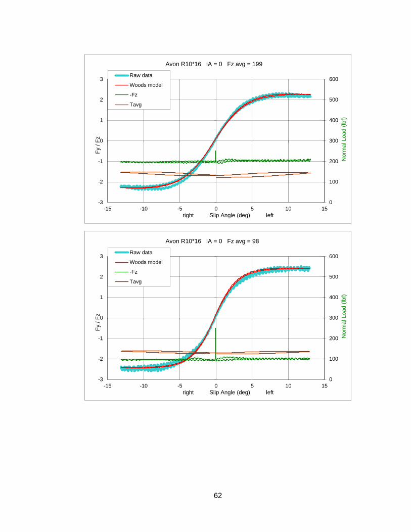
Avon R10*16 IA = 0 Fz avg = 199
Raw data
Woods model
-Fz
Tavg
0
100
200
300
400
500
600
-3
-2
-1
0
1
2
3
-15 -10 -5 0 5 10 15
Norm
al Load (
lbf)
Fy /
Fz
right Slip Angle (deg) left
Avon R10*16 IA = 0 Fz avg = 98
Raw data
Woods model
-Fz
Tavg

63
0
100
200
300
400
500
600
-3
-2
-1
0
1
2
3
-15 -10 -5 0 5 10 15
Norm
al Load (
lbf)
Fy /
Fz
right Slip Angle (deg) left
Avon R10*16 IA = 0 Fz avg = 47
Raw data
Woods model
-Fz
Tavg
0
100
200
300
400
500
600
-3
-2
-1
0
1
2
3
-15 -10 -5 0 5 10 15
Norm
al Load (
lbf)
Fy /
Fz
right Slip Angle (deg) left
Avon R10*16 IA = 2 Fz avg = 249
Raw data
Woods model
-Fz
Tavg

64
0
100
200
300
400
500
600
-3
-2
-1
0
1
2
3
-15 -10 -5 0 5 10 15
Norm
al Load (
lbf)
Fy /
Fz
right Slip Angle (deg) left
Avon R10*16 IA = 2 Fz avg = 197
Raw data
Woods model
-Fz
Tavg
0
100
200
300
400
500
600
-3
-2
-1
0
1
2
3
-15 -10 -5 0 5 10 15
Norm
al Load (
lbf)
Fy /
Fz
right Slip Angle (deg) left
Avon R10*16 IA = 2 Fz avg = 99
Raw data
Woods model
-Fz
Tavg
65
0
100
200
300
400
500
600
-3
-2
-1
0
1
2
3
-15 -10 -5 0 5 10 15
Norm
al Load (
lbf)
Fy /
Fz
right Slip Angle (deg) left
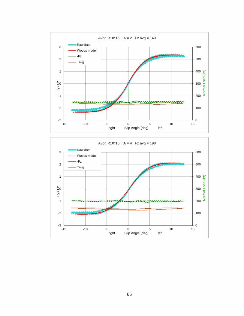
Avon R10*16 IA = 2 Fz avg = 149
Raw data
Woods model
-Fz
Tavg
0
100
200
300
400
500
600
-3
-2
-1
0
1
2
3
-15 -10 -5 0 5 10 15
Norm
al Load (
lbf)
Fy /
Fz
right Slip Angle (deg) left
Avon R10*16 IA = 4 Fz avg = 198
Raw data
Woods model
-Fz
Tavg

66
0
100
200
300
400
500
600
-3
-2
-1
0
1
2
3
-15 -10 -5 0 5 10 15
Norm
al Load (
lbf)
Fy /
Fz
right Slip Angle (deg) left
Avon R10*16 IA = 4 Fz avg = 48
Raw data
Woods model
-Fz
Tavg
0
100
200
300
400
500
600
-3
-2
-1
0
1
2
3
-15 -10 -5 0 5 10 15
Norm
al Load (
lbf)
Fy /
Fz
right Slip Angle (deg) left
Avon R10*16 IA = 4 Fz avg = 250
Raw data
Woods model
-Fz
Tavg

67
0
100
200
300
400
500
600
-3
-2
-1
0
1
2
3
-15 -10 -5 0 5 10 15
Norm
al Load (
lbf)
Fy /
Fz
right Slip Angle (deg) left
Avon R10*16 IA = 4 Fz avg = 99
Raw data
Woods model
-Fz
Tavg
120
130
140
150
160
170
180
0.0
0.5
1.0
1.5
2.0
2.5
3.0
0 50 100 150 200 250 300
Te
mpera
ture
(deg F
)
Mu
y
Normal Load (lbf)
Avon R10*16
μ+
-μ-
mu fit +
mu fit-
T+
T-
T fit
IA = 0 deg

68
0
2
4
6
8
10
12
14
16
18
20
22
24
26
28
2
4
6
8
10
12
14
16
0 50 100 150 200 250 300
g
A p
eak
Normal Load (lbf)
Avon R10*16α +
-α -
a+ fit
a- fit
g
g fit
IA = 0 deg
120
130
140
150
160
170
180
0.0
0.5
1.0
1.5
2.0
2.5
3.0
0 50 100 150 200 250 300
Te
mpera
ture
(deg F
)
Mu
y
Normal Load (lbf)
Avon R10*16
μ+
-μ-
mu fit +
mu fit -
T+
T-
T fit
IA = 1 deg

69
120
130
140
150
160
170
180
0.0
0.5
1.0
1.5
2.0
2.5
3.0
0 50 100 150 200 250 300
Te
mp
era
ture
(d
eg
F)
Muy
Normal Load (lbf)
Avon R10*16
μ+
-μ-
mu fit +
mu fit -
T+
T-
T fit
IA = 2 deg
0
2
4
6
8
10
12
14
16
18
20
22
24
26
28
2
4
6
8
10
12
14
16
0 50 100 150 200 250 300
g
A p
eak
Normal Load (lbf)
Avon R10*16α +
-α -
a+ fit
a- fit
g
g fit
IA = 1 deg

70
0
2
4
6
8
10
12
14
16
18
20
22
24
26
28
2
4
6
8
10
12
14
16
0 50 100 150 200 250 300
g
A p
eak
Normal Load (lbf)
Avon R10*16
α +
-α -
a+ fit
a- fit
g
g fit
IA = 2 deg
6
7
8
9
10
11
12
-6 -4 -2 0 2 4 6
A p
eak
Camber (deg)
Avon R10*16
αpeak 50
αpeak 150
αpeak 250
αpeak 350
αpeak 450
apeak fit

71
0.0
0.5
1.0
1.5
2.0
2.5
3.0
-5 -3 -1 1 3 5
Mu p
eak
Camber (deg)
Avon R10*16
μpeak 50
μpeak 150
μpeak 250
μpeak 350
μpeak 450
Upeak fit
-0.3
-0.2
-0.1
0.0
0.1
0.2
0.3
0.4
0 50 100 150 200 250 300
A o
ff (
deg)
Normal Load (lbf)
Avon R10*16
0
2
4
fit

72
Goodyear 20x7-13 D2509
0
100
200
300
400
500
600
-3
-2
-1
0
1
2
3
-15 -10 -5 0 5 10 15
Norm
al Load (
lbf)
Fy /
Fz
right Slip Angle (deg) left
Run 3 Goodyear 20x7-13 D2509 IA = 0 Fz avg = 47Raw data
Woods model
-Fz
Tavg
0
100
200
300
400
500
600
-3
-2
-1
0
1
2
3
-15 -10 -5 0 5 10 15
No
rma
l L
oa
d (
lbf)
Fy /
Fz
right Slip Angle (deg) left
Run 3 Goodyear 20x7-13 D2509 IA = 1 Fz avg = 47Raw data
Woods model
-Fz
Tavg

73
0
100
200
300
400
500
600
-3
-2
-1
0
1
2
3
-15 -10 -5 0 5 10 15
Norm
al Load (
lbf)
Fy /
Fz
right Slip Angle (deg) left
Run 3 Goodyear 20x7-13 D2509 IA = 2 Fz avg = 47
Raw data
Woods model
-Fz
Tavg
0
100
200
300
400
500
600
-3
-2
-1
0
1
2
3
-15 -10 -5 0 5 10 15
Norm
al Load (
lbf)
Fy /
Fz
right Slip Angle (deg) left
Run 3 Goodyear 20x7-13 D2509 IA = 3 Fz avg = 49Raw data
Woods model
-Fz
Tavg

74
0
100
200
300
400
500
600
-3
-2
-1
0
1
2
3
-15 -10 -5 0 5 10 15
Norm
al Load (
lbf)
Fy /
Fz
right Slip Angle (deg) left
Run 3 Goodyear 20x7-13 D2509 IA = 4 Fz avg = 49
Fy/Fz model
-Fz
Tavg
0
100
200
300
400
500
600
-3
-2
-1
0
1
2
3
-15 -10 -5 0 5 10 15
Norm
al Load (
lbf)
Fy /
Fz
right Slip Angle (deg) left
Run 3 Goodyear 20x7-13 D2509 IA = 0 Fz avg = 147
Raw data
Woods model
-Fz
Tavg

75
0
100
200
300
400
500
600
-3
-2
-1
0
1
2
3
-15 -10 -5 0 5 10 15
No
rma
l L
oa
d (
lbf)
Fy /
Fz
right Slip Angle (deg) left
Run 3 Goodyear 20x7-13 D2509 IA = 1 Fz avg = 147Raw data
Woods model
-Fz
Tavg
0
100
200
300
400
500
600
-3
-2
-1
0
1
2
3
-15 -10 -5 0 5 10 15
Norm
al Load (
lbf)
Fy /
Fz
right Slip Angle (deg) left
Run 3 Goodyear 20x7-13 D2509 IA = 2 Fz avg = 147Raw data
Woods model
-Fz
Tavg

76
0
100
200
300
400
500
600
-3
-2
-1
0
1
2
3
-15 -10 -5 0 5 10 15
Norm
al Load (
lbf)
Fy /
Fz
right Slip Angle (deg) left
Run 3 Goodyear 20x7-13 D2509 IA = 3 Fz avg = 149Raw data
Woods model
-Fz
Tavg
0
100
200
300
400
500
600
-3
-2
-1
0
1
2
3
-15 -10 -5 0 5 10 15
Norm
al Load (
lbf)
Fy /
Fz
right Slip Angle (deg) left
Run 3 Goodyear 20x7-13 D2509 IA = 4 Fz avg = 150Raw data
Woods model
-Fz
Tavg
77
0
100
200
300
400
500
600
-3
-2
-1
0
1
2
3
-15 -10 -5 0 5 10 15
Norm
al Load (
lbf)
Fy /
Fz
right Slip Angle (deg) left
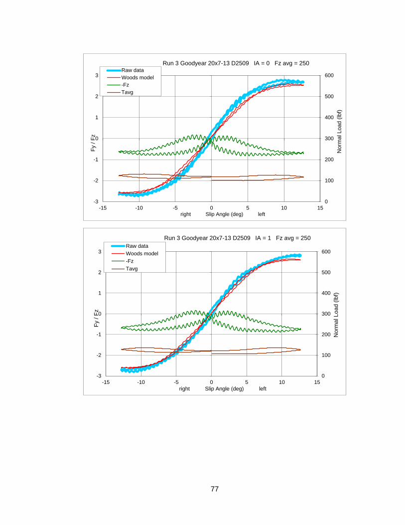
Run 3 Goodyear 20x7-13 D2509 IA = 0 Fz avg = 250Raw data
Woods model
-Fz
Tavg
0
100
200
300
400
500
600
-3
-2
-1
0
1
2
3
-15 -10 -5 0 5 10 15
No
rma
l L
oa
d (
lbf)
Fy /
Fz
right Slip Angle (deg) left
Run 3 Goodyear 20x7-13 D2509 IA = 1 Fz avg = 250
Raw data
Woods model
-Fz
Tavg

78
0
100
200
300
400
500
600
-3
-2
-1
0
1
2
3
-15 -10 -5 0 5 10 15
Norm
al Load (
lbf)
Fy /
Fz
right Slip Angle (deg) left
Run 3 Goodyear 20x7-13 D2509 IA = 2 Fz avg = 251Raw data
Woods model
-Fz
Tavg
0
100
200
300
400
500
600
-3
-2
-1
0
1
2
3
-15 -10 -5 0 5 10 15
Norm
al Load (
lbf)
Fy /
Fz
right Slip Angle (deg) left
Run 3 Goodyear 20x7-13 D2509 IA = 3 Fz avg = 251Raw data
Woods model
-Fz
Tavg

79
0
100
200
300
400
500
600
-3
-2
-1
0
1
2
3
-15 -10 -5 0 5 10 15
Norm
al Load (
lbf)
Fy /
Fz
right Slip Angle (deg) left
Run 3 Goodyear 20x7-13 D2509 IA = 4 Fz avg = 251
Raw data
Woods model
-Fz
Tavg
0
100
200
300
400
500
600
-3
-2
-1
0
1
2
3
-15 -10 -5 0 5 10 15
Norm
al Load (
lbf)
Fy /
Fz
right Slip Angle (deg) left
Run 3 Goodyear 20x7-13 D2509 IA = 0 Fz avg = 355
Raw data
Woods model
-Fz
Tavg

80
0
100
200
300
400
500
600
-3
-2
-1
0
1
2
3
-15 -10 -5 0 5 10 15
No
rma
l L
oa
d (
lbf)
Fy /
Fz
right Slip Angle (deg) left
Run 3 Goodyear 20x7-13 D2509 IA = 1 Fz avg = 352
Raw data
Woods model
-Fz
Tavg
0
100
200
300
400
500
600
-3
-2
-1
0
1
2
3
-15 -10 -5 0 5 10 15
Norm
al Load (
lbf)
Fy /
Fz
right Slip Angle (deg) left
Run 3 Goodyear 20x7-13 D2509 IA = 2 Fz avg = 355
Raw data
Woods model
-Fz
Tavg

81
0
100
200
300
400
500
600
-3
-2
-1
0
1
2
3
-15 -10 -5 0 5 10 15
Norm
al Load (
lbf)
Fy /
Fz
right Slip Angle (deg) left
Run 3 Goodyear 20x7-13 D2509 IA = 4 Fz avg = 356
Raw data
Woods model
-Fz
Tavg
0
100
200
300
400
500
600
-3
-2
-1
0
1
2
3
-15 -10 -5 0 5 10 15
Norm
al Load (
lbf)
Fy /
Fz
right Slip Angle (deg) left
Run 3 Goodyear 20x7-13 D2509 IA = 0 Fz avg = 459Raw data
Woods model
-Fz
Tavg

82
0
100
200
300
400
500
600
-3
-2
-1
0
1
2
3
-15 -10 -5 0 5 10 15
Norm
al Load (
lbf)
Fy /
Fz
right Slip Angle (deg) left
Run 3 Goodyear 20x7-13 D2509 IA = 1 Fz avg = 460Raw data
Woods model
-Fz
Tavg
0
100
200
300
400
500
600
-3
-2
-1
0
1
2
3
-15 -10 -5 0 5 10 15
Norm
al Load (
lbf)
Fy /
Fz
right Slip Angle (deg) left
Run 3 Goodyear 20x7-13 D2509 IA = 2 Fz avg = 461Raw data
Woods model
-Fz
Tavg

83
0
100
200
300
400
500
600
-3
-2
-1
0
1
2
3
-15 -10 -5 0 5 10 15
Norm
al Load (
lbf)
Fy /
Fz
right Slip Angle (deg) left
Run 3 Goodyear 20x7-13 D2509 IA = 3 Fz avg = 462Raw data
Woods model
-Fz
Tavg
0
100
200
300
400
500
600
-3
-2
-1
0
1
2
3
-15 -10 -5 0 5 10 15
Norm
al Load (
lbf)
Fy /
Fz
right Slip Angle (deg) left
Run 3 Goodyear 20x7-13 D2509 IA = 4 Fz avg = 463Raw data
Woods model
-Fz
Tavg
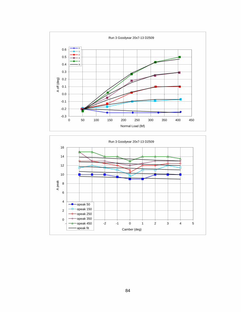
84
-0.3
-0.2
-0.1
0.0
0.1
0.2
0.3
0.4
0.5
0.6
0 50 100 150 200 250 300 350 400 450
A o
ff (
deg)
Normal Load (lbf)
Run 3 Goodyear 20x7-13 D2509
0
1
2
3
4
fit
0
2
4
6
8
10
12
14
16
-5 -4 -3 -2 -1 0 1 2 3 4 5
A p
eak
Camber (deg)
Run 3 Goodyear 20x7-13 D2509
αpeak 50
αpeak 150
αpeak 250
αpeak 350
αpeak 450
apeak fit

85
0.0
0.5
1.0
1.5
2.0
2.5
3.0
3.5
-6 -4 -2 0 2 4 6
Mu p
eak
Camber (deg)
Run 3 Goodyear 20x7-13 D2509
μpeak 50
μpeak 150
μpeak 250
μpeak 350
μpeak 450
upeak fit
90
100
110
120
130
140
150
0.0
0.5
1.0
1.5
2.0
2.5
3.0
0 100 200 300 400 500
Te
mpera
ture
(deg F
)
Mu
y
Normal Load (lbf)
Run 3 Goodyear 20x7-13 D2509
μ+
-μ-
mu fit+
mufit-
IA = 0 deg

86
90
100
110
120
130
140
150
0.0
0.5
1.0
1.5
2.0
2.5
3.0
0 100 200 300 400 500
Te
mpera
ture
(deg F
)
Mu
y
Normal Load (lbf)
Run 3 Goodyear 20x7-13 D2509
μ+
-μ-
mu fit+
mu fit-
IA = 1 deg
90
100
110
120
130
140
150
0.0
0.5
1.0
1.5
2.0
2.5
3.0
0 100 200 300 400 500
Te
mp
era
ture
(d
eg
F)
Muy
Normal Load (lbf)
Run 3 Goodyear 20x7-13 D2509
μ+
-μ-
mu fit+
mu fit-
IA = 2 deg

87
90
100
110
120
130
140
150
0.0
0.5
1.0
1.5
2.0
2.5
3.0
0 100 200 300 400 500
Te
mpera
ture
(deg F
)
Mu
y
Normal Load (lbf)
Run 3 Goodyear 20x7-13 D2509
μ+
-μ-
mu fit+mu fit-
IA = 3 deg
90
100
110
120
130
140
150
0.0
0.5
1.0
1.5
2.0
2.5
3.0
0 100 200 300 400 500
Te
mpera
ture
(deg F
)
Mu
y
Normal Load (lbf)
Run 3 Goodyear 20x7-13 D2509
μ+
-μ-
mu fi+mufit -
IA = 4 deg

88
0
2
4
6
8
10
12
14
16
18
20
22
24
26
28
2
4
6
8
10
12
14
16
0 100 200 300 400 500
g
A p
eak
Normal Load (lbf)
Run 3 Goodyear 20x7-13 D2509α +
-α -
a+fita-fit
IA = 0 deg
0
2
4
6
8
10
12
14
16
18
20
22
24
26
28
2
4
6
8
10
12
14
16
0 100 200 300 400 500
g
A p
eak
Normal Load (lbf)
Run 3 Goodyear 20x7-13 D2509α +
-α -
a+fita-fit
IA = 1 deg

89
0
2
4
6
8
10
12
14
16
18
20
22
24
26
28
2
4
6
8
10
12
14
16
0 100 200 300 400 500
g
A p
eak
Normal Load (lbf)
Run 3 Goodyear 20x7-13 D2509
α +
-α -
a+fita-fit
IA = 2 deg
0
2
4
6
8
10
12
14
16
18
20
22
24
26
28
2
4
6
8
10
12
14
16
0 100 200 300 400 500
g
A p
eak
Normal Load (lbf)
Run 3 Goodyear 20x7-13 D2509
α +
-α -
a+fita-fit
IA = 3 deg

90
Hoosier R13 20.5*7 R25B
0
2
4
6
8
10
12
14
16
18
20
22
24
26
28
2
4
6
8
10
12
14
16
0 100 200 300 400 500
g
A p
eak
Normal Load (lbf)
Run 3 Goodyear 20x7-13 D2509
α +
-α -
a+fita-fit
IA = 4 deg
0
100
200
300
400
500
600
-3
-2
-1
0
1
2
3
-15 -10 -5 0 5 10 15
Norm
al Load (
lbf)
Fy /
Fz
right Slip Angle (deg) left
Hoosier R13 20.5*7 R25B IA = 0 Fz avg = 250Raw data
Woods model
-Fz
Tavg

91
0
100
200
300
400
500
600
-3
-2
-1
0
1
2
3
-15 -10 -5 0 5 10 15
No
rma
l L
oa
d (
lbf)
Fy /
Fz
right Slip Angle (deg) left
Hoosier R13 20.5*7 R25B IA = 1 Fz avg = 251Raw data
Woods model
-Fz
Tavg
0
100
200
300
400
500
600
-3
-2
-1
0
1
2
3
-15 -10 -5 0 5 10 15
Norm
al Load (
lbf)
Fy /
Fz
right Slip Angle (deg) left
Hoosier R13 20.5*7 R25B IA = 2 Fz avg = 252Raw data
Woods model
-Fz
Tavg

92
0
100
200
300
400
500
600
-3
-2
-1
0
1
2
3
-15 -10 -5 0 5 10 15
Norm
al Load (
lbf)
Fy /
Fz
right Slip Angle (deg) left
Hoosier R13 20.5*7 R25B IA = 3 Fz avg = 253
Raw data
Woods model
-Fz
Tavg
0
100
200
300
400
500
600
-3
-2
-1
0
1
2
3
-15 -10 -5 0 5 10 15
Norm
al Load (
lbf)
Fy /
Fz
right Slip Angle (deg) left
Hoosier R13 20.5*7 R25B IA = 4 Fz avg = 253Raw data
Woods model
-Fz
Tavg

93
0
100
200
300
400
500
600
-3
-2
-1
0
1
2
3
-15 -10 -5 0 5 10 15
Norm
al Load (
lbf)
Fy /
Fz
right Slip Angle (deg) left
Hoosier R13 20.5*7 R25B IA = 0 Fz avg = 150
Raw data
Woods model
-Fz
Tavg
0
100
200
300
400
500
600
-3
-2
-1
0
1
2
3
-15 -10 -5 0 5 10 15
No
rma
l L
oa
d (
lbf)
Fy /
Fz
right Slip Angle (deg) left
Hoosier R13 20.5*7 R25B IA = 1 Fz avg = 151
Raw data
Woods model
-Fz
Tavg

94
0
100
200
300
400
500
600
-3
-2
-1
0
1
2
3
-15 -10 -5 0 5 10 15
Norm
al Load (
lbf)
Fy /
Fz
right Slip Angle (deg) left
Hoosier R13 20.5*7 R25B IA = 2 Fz avg = 151
Raw data
Woods model
-Fz
Tavg
0
100
200
300
400
500
600
-3
-2
-1
0
1
2
3
-15 -10 -5 0 5 10 15
Norm
al Load (
lbf)
Fy /
Fz
right Slip Angle (deg) left
Hoosier R13 20.5*7 R25B IA = 3 Fz avg = 152Raw data
Woods model
-Fz
Tavg

95
0
100
200
300
400
500
600
-3
-2
-1
0
1
2
3
-15 -10 -5 0 5 10 15
Norm
al Load (
lbf)
Fy /
Fz
right Slip Angle (deg) left
Hoosier R13 20.5*7 R25B IA = 4 Fz avg = 152Raw data
Woods model
-Fz
Tavg
0
100
200
300
400
500
600
-3
-2
-1
0
1
2
3
-15 -10 -5 0 5 10 15
Norm
al Load (
lbf)
Fy /
Fz
right Slip Angle (deg) left
Hoosier R13 20.5*7 R25B IA = 0 Fz avg = 99Raw data
Woods model
-Fz
Tavg

96
0
100
200
300
400
500
600
-3
-2
-1
0
1
2
3
-15 -10 -5 0 5 10 15
No
rma
l L
oa
d (
lbf)
Fy /
Fz
right Slip Angle (deg) left
Hoosier R13 20.5*7 R25B IA = 1 Fz avg = 99
Raw data
Woods model
-Fz
Tavg
0
100
200
300
400
500
600
-3
-2
-1
0
1
2
3
-15 -10 -5 0 5 10 15
Norm
al Load (
lbf)
Fy /
Fz
right Slip Angle (deg) left
Hoosier R13 20.5*7 R25B IA = 2 Fz avg = 100Raw data
Woods model
-Fz
Tavg

97
0
100
200
300
400
500
600
-3
-2
-1
0
1
2
3
-15 -10 -5 0 5 10 15
Norm
al Load (
lbf)
Fy /
Fz
right Slip Angle (deg) left
Hoosier R13 20.5*7 R25B IA = 3 Fz avg = 102
Raw data
Woods model
-Fz
Tavg
0
100
200
300
400
500
600
-3
-2
-1
0
1
2
3
-15 -10 -5 0 5 10 15
Norm
al Load (
lbf)
Fy /
Fz
right Slip Angle (deg) left
Hoosier R13 20.5*7 R25B IA = 4 Fz avg = 101Raw data
Woods model
-Fz
Tavg

98
0
100
200
300
400
500
600
-3
-2
-1
0
1
2
3
-15 -10 -5 0 5 10 15
Norm
al Load (
lbf)
Fy /
Fz
right Slip Angle (deg) left
Hoosier R13 20.5*7 R25B IA = 0 Fz avg = 48
Raw data
Woods model
-Fz
Tavg
0
100
200
300
400
500
600
-3
-2
-1
0
1
2
3
-15 -10 -5 0 5 10 15
Norm
al Load (
lbf)
Fy /
Fz
right Slip Angle (deg) left
Hoosier R13 20.5*7 R25B IA = 1 Fz avg = 49Raw data
Woods model
-Fz
Tavg

99
0
100
200
300
400
500
600
-3
-2
-1
0
1
2
3
-15 -10 -5 0 5 10 15
No
rma
l L
oa
d (
lbf)
Fy /
Fz
right Slip Angle (deg) left
Hoosier R13 20.5*7 R25B IA = 2 Fz avg = 49Raw data
Woods model
-Fz
Tavg
0
100
200
300
400
500
600
-3
-2
-1
0
1
2
3
-15 -10 -5 0 5 10 15
Norm
al Load (
lbf)
Fy /
Fz
right Slip Angle (deg) left
Hoosier R13 20.5*7 R25B IA = 3 Fz avg = 51Raw data
Woods model
-Fz
Tavg

100
0
100
200
300
400
500
600
-3
-2
-1
0
1
2
3
-15 -10 -5 0 5 10 15
Norm
al Load (
lbf)
Fy /
Fz
right Slip Angle (deg) left
Hoosier R13 20.5*7 R25B IA = 4 Fz avg = 50Raw data
Woods model
-Fz
Tavg
120
130
140
150
160
170
180
0.0
0.5
1.0
1.5
2.0
2.5
3.0
0 50 100 150 200 250 300
Te
mpera
ture
(deg F
)
Mu
y
Normal Load (lbf)
Run 3 Hoosier 20.5*7*13 R25B
μ+
-μ-
mu fit+mu fit -
T+
IA = 1 deg

101
120
130
140
150
160
170
180
0.0
0.5
1.0
1.5
2.0
2.5
3.0
0 50 100 150 200 250 300
Te
mp
era
ture
(d
eg
F)
Muy
Normal Load (lbf)
Run 3 Hoosier 20.5*7*13 R25B
μ+
-μ-
mu fit+mu fit-T+
IA = 2 deg
120
130
140
150
160
170
180
0.0
0.5
1.0
1.5
2.0
2.5
3.0
0 50 100 150 200 250 300
Te
mpera
ture
(deg F
)
Mu
y
Normal Load (lbf)
Run 3 Hoosier 20.5*7*13 R25B
μ+
-μ-
mu fit+mu fit-T+
IA = 3 deg

102
120
130
140
150
160
170
180
0.0
0.5
1.0
1.5
2.0
2.5
3.0
0 50 100 150 200 250 300
Te
mpera
ture
(deg F
)
Mu
y
Normal Load (lbf)
Run 3 Hoosier 20.5*7*13 R25B
μ+
-μ-
mu fi+mufit -
IA = 4 deg
0
2
4
6
8
10
12
14
16
18
20
22
24
26
28
2
4
6
8
10
12
14
16
0 50 100 150 200 250 300
g
A p
eak
Normal Load (lbf)
Run 3 Hoosier 20.5*7*13 R25B α +
-α -
a+ fit
a- fit
g
g fit
IA = 0 deg

103
0
2
4
6
8
10
12
14
16
18
20
22
24
26
28
2
4
6
8
10
12
14
16
0 50 100 150 200 250 300
g
A p
eak
Normal Load (lbf)
Run 3 Hoosier 20.5*7*13 R25B
α +
-α -
a+ fit
a- fit
g
g fit
IA = 1 deg
0
2
4
6
8
10
12
14
16
18
20
22
24
26
28
2
4
6
8
10
12
14
16
0 50 100 150 200 250 300
g
A p
eak
Normal Load (lbf)
Run 3 Hoosier 20.5*7*13 R25B
α +
-α -
a+ fit
a- fit
g
g fit
IA = 2 deg

104
0
2
4
6
8
10
12
14
16
18
20
22
24
26
28
2
4
6
8
10
12
14
16
0 50 100 150 200 250 300
g
A p
eak
Normal Load (lbf)
Run 3 Hoosier 20.5*7*13 R25B
α +
-α -
a+ fit
a- fit
g
g fit
IA = 3 deg
0
2
4
6
8
10
12
14
16
18
20
22
24
26
28
2
4
6
8
10
12
14
16
0 50 100 150 200 250 300
g
A p
eak
Normal Load (lbf)
Run 3 Hoosier 20.5*7*13 R25B
α +
-α -
a+ fit
a- fit
g
g fit
IA = 4 deg

105
120
130
140
150
160
170
180
0.0
0.5
1.0
1.5
2.0
2.5
3.0
0 50 100 150 200 250 300
Te
mpera
ture
(deg F
)
Muy
Normal Load (lbf)
Run 3 Hoosier 20.5*7*13 R25B
μ+
-μ-
mu fit+mu fit-
T+
IA = 0 deg
0
2
4
6
8
10
12
14
16
18
20
22
24
26
28
2
4
6
8
10
12
14
16
0 50 100 150 200 250 300
g
A p
eak
Normal Load (lbf)
Run 3 Hoosier 20.5*7*13 R25B α +
-α -
a+ fit
a- fit
g
g fit
IA = 0 deg

106
120
130
140
150
160
170
180
0.0
0.5
1.0
1.5
2.0
2.5
3.0
0 50 100 150 200 250 300
Te
mpera
ture
(deg F
)
Mu
y
Normal Load (lbf)
Run 3 Hoosier 20.5*7*13 R25B
μ+
-μ-
mu fit+mu fit -
T+
IA = 1 deg
120
130
140
150
160
170
180
0.0
0.5
1.0
1.5
2.0
2.5
3.0
0 50 100 150 200 250 300
Te
mp
era
ture
(d
eg
F)
Mu
y
Normal Load (lbf)
Run 3 Hoosier 20.5*7*13 R25B
μ+
-μ-
mu fit+mu fit-T+
IA = 2 deg

107
0
2
4
6
8
10
12
14
16
18
20
22
24
26
28
2
4
6
8
10
12
14
16
0 50 100 150 200 250 300
g
A p
eak
Normal Load (lbf)
Run 3 Hoosier 20.5*7*13 R25B
α +
-α -
a+ fit
a- fit
g
g fit
IA = 1 deg
0
2
4
6
8
10
12
14
16
18
20
22
24
26
28
2
4
6
8
10
12
14
16
0 50 100 150 200 250 300
g
A p
eak
Normal Load (lbf)
Run 3 Hoosier 20.5*7*13 R25B
α +
-α -
a+ fit
a- fit
g
g fit
IA = 2 deg

108
0
2
4
6
8
10
12
14
16
18
20
22
24
26
28
2
4
6
8
10
12
14
16
0 50 100 150 200 250 300
g
A p
eak
Normal Load (lbf)
Run 3 Hoosier 20.5*7*13 R25B
α +
-α -
a+ fit
a- fit
g
g fit
IA = 3 deg
120
130
140
150
160
170
180
0.0
0.5
1.0
1.5
2.0
2.5
3.0
0 50 100 150 200 250 300
Te
mpera
ture
(deg F
)
Mu
y
Normal Load (lbf)
Run 3 Hoosier 20.5*7*13 R25B
μ+
-μ-
mu fit+mu fit-T+
IA = 3 deg

109
120
130
140
150
160
170
180
0.0
0.5
1.0
1.5
2.0
2.5
3.0
0 50 100 150 200 250 300
Te
mpera
ture
(deg F
)
Mu
y
Normal Load (lbf)
Run 3 Hoosier 20.5*7*13 R25B
μ+
-μ-
mu fi+mufit -
IA = 4 deg
0
2
4
6
8
10
12
14
16
18
20
22
24
26
28
2
4
6
8
10
12
14
16
0 50 100 150 200 250 300
g
A p
eak
Normal Load (lbf)
Run 3 Hoosier 20.5*7*13 R25B
α +
-α -
a+ fit
a- fit
g
g fit
IA = 4 deg

110
5
6
7
8
9
10
11
12
-6 -4 -2 0 2 4 6
A p
eak
Camber (deg)
Run 3 Hoosier 20.5*7*13 R25B
αpeak 50
αpeak 100
αpeak 150
-0.1
0.0
0.1
0.2
0.3
0.4
0.5
0.6
0.7
0 50 100 150 200 250 300
A o
ff (
deg)
Normal Load (lbf)
Run 3 Hoosier 20.5*7*13 R25B
0
1
2
3
4
fit

111
0.0
0.5
1.0
1.5
2.0
2.5
3.0
3.5
-6 -4 -2 0 2 4 6
Mu p
eak
Camber (deg)
Run 3 Hoosier 20.5*7*13 R25B
μpeak 50
μpeak 100
μpeak 150
μpeak 250
upeak fit

112
References
[1] W. F. Milliken and D. L. Milliken, “Race Car Vehicle Dynamics,” Race, vol. 1. p. 1000, 1995.
[2] R. Woods, “Normalization of the Pacejka Tire Model,” SAE Technical Paper, no. 724. 2004.
[3] M. Schmid, “Tire Modeling for Multibody Dynamics Applications,” p. 62, 2011.
[4] N. York and A. Engineering, “Extension of the Nondimensional Tire Theory To,” no.
December, 2006.
[5] E. M. (University A. B. Kasprzak and D. (Calspan C. . Gentz, “The Formula SAE Tire Test
Consortium — Tire Testing and Data Handling,” Soc. Automot. Eng., no. 724, p. 12, 2006.
[6] N. J. Trevorrow, “Development of a Dynamic Force Model for Racing Slick Tyres,”
Measurement, no. Figure 1, pp. 1–17, 1995.