CRANFIELD UNIVERSITY

INYIAMA, FIDELIS CHIDOZIE

ACTIVE CONTROL OF HYDRODYNAMIC SLUG FLOW

Department of Offshore, Process Systems and Energy

Engineering

MSc by Research

Academic Year: 2012 - 2013

Supervisor: Dr. Yi Cao

April, 2013

CRANFIELD UNIVERSITY

SCHOOL OF ENGINEERING

Department of Offshore, Process Systems and Energy Engineering

MSc by Research

Academic Year 2012- 2013

INYIAMA, FIDELIS CHIDOZIE

ACTIVE CONTROL OF HYDRODYNAMIC SLUG FLOW

Supervisor: Dr. Yi Cao

April, 2013

© Cranfield University 2013. All rights reserved. No part of this

publication may be reproduced without the written permission of the

copyright owner.

i

ABSTRACT

Multiphase flow is associated with concurrent flow of more than one phase

(gas-liquid, liquid-solid, or gas-liquid-solid) in a conduit. The simultaneous flow

of these phases in a flow line, may initiate a slug flow in the pipeline.

Hydrodynamic slug flow is an alternate or irregular flow with surges of liquid

slug and gas pocket. This occurs when the velocity difference between the gas

flow rate and liquid flow rate is high enough resulting in an unstable

hydrodynamic behaviour usually caused by the Kelvin-Helmholtz instability.

Active feedback control technology, though found effective for the control of

severe slugs, has not been studied for hydrodynamic slug mitigation in the

literature. This work extends active feedback control application for mitigating

hydrodynamic slug problem to enhance oil production and recovery.

Active feedback Proportional-Integral (PI) control strategy based on

measurement of pressure at the riser base as controlled variable with topside

choking as manipulated variable was investigated through Olga simulation in

this project. A control system that uses the topside choke valve to keep the

pressure at the riser base at or below the average pressure in the riser slug

cycle has been implemented. This has been found to prevent liquid

accumulation or blockage of the flow line.

OLGA (olga is a commercial software widely tested and used in oil and gas

industries) has been used to assess the capability of active feedback control

strategy for hydrodynamic slug control and has been found to give useful results

and most interestingly the increase in oil production and recovery. The riser

slugging was suppressed and the choke valve opening was improved from 5%

to 12.65% using riser base pressure as controlled variable and topside choke

valve as the manipulated variable for the manual choking when compared to the

automatic choking in a stabilised operation, representing an improvement of

7.65% in the valve opening. Secondly, implementing active control at open-loop

condition reduced the riser base pressure from 15.3881bara to 13.4016bara.

ii

Keywords:

Choking, multiphase, flow regime, feedback control, close-loop, open-loop,

bifurcation map, OLGA

iii

ACKNOWLEDGEMENTS

As I write the thesis for this work, I found myself looking back on the learning

experience, both personally and professionally because of the challenges it

presented and the opportunity of learning from knowledgeable people.

My sincere appreciation goes to my supervisor Dr Yi Cao for introducing me to

this area of study. His support, encouragement and patience in guiding me

through this period are greatly valued. I have gained from his wealth of

experience. I also wish to thank the Head of Process Systems Engineering

Group Prof Hoi Yeung for his fatherly advice when I needed them most. The

entire Staff of Process Systems Engineering Group deserves commendation,

particularly Sam Skears (Research programme & Short Course Manager,

School of Engineering) for her organisation and timely communication.

My special thanks go to my sponsors, Tertiary Education Trust Fund (TETF)

and Enugu State University of Science and Technology (ESUT), Nigeria for

giving me the opportunity to embark on the training.

I wish to also appreciate my friends and colleagues Dr Crips Alison, Solomon

Alagbe, Adegboyega Ehinmowo, Archibong Eso Archibong, David Okuonrobo,

Xin of SPT, Sunday Kanshio and Ndubuisi Okereke for their support and

encouragement. My family in diaspora, Holding Forth the Word Ministry

(HFWM) and Cranfield Pentecostal Assembly (CPA) is highly appreciated for

the love we share.

My sincere gratitude goes to my love Abigail and children Chimdindu and

Chiedozie and the entire members of the family for their sacrifice. I missed your

warmth during this period of my absence. Engr Emeka Ojiogu deserves special

thanks for being to me a worthy friend. I appreciate you all and I pray God

Almighty to bless your endeavours according to His riches in glory.

Accept my appreciation.

v

TABLE OF CONTENTS

ABSTRACT ......................................................................................................... i

ACKNOWLEDGEMENTS................................................................................... iii

LIST OF FIGURES ........................................................................................... viii

LIST OF TABLES ............................................................................................... x

LIST OF ABBREVIATIONS ................................................................................ xi

1 INTRODUCTION ............................................................................................. 1

1.1 Background ............................................................................................... 1

1.2 Hydrodynamic Slugging ............................................................................ 3

1.3 Why is Slugging a Problem? ..................................................................... 5

1.4 Compare mechanisms of Hydrodynamic and Severe Slugs. .................... 6

1.5 Operation Induced Slugging ..................................................................... 9

1.6 Slug Mitigation and Prevention Methods ................................................... 9

1.7 Aim. ......................................................................................................... 10

1.8 Objectives. .............................................................................................. 10

1.9 Conclusion .............................................................................................. 10

2 LITERATURE REVIEW ................................................................................. 13

2.1 Multiphase Flow ...................................................................................... 13

2.2 Flow Regime Determination .................................................................... 14

2.2.1 Flow Regime Map in Horizontal Pipe ............................................... 14

2.3 Prediction of Flow Regime Transition in Horizontal Pipes ....................... 15

2.3.1 Transition from Stratified Flow .......................................................... 15

2.3.2 Transition to Annular Flow ................................................................ 16

2.3.3 Transition to Dispersed Bubble Flow ................................................ 17

2.4 Flow Regime in Vertical Pipes ................................................................ 17

2.5 Vertical Pipe Flow Regime Map .............................................................. 19

2.5.1 Transition from Bubble to Slug Flow ................................................ 19

2.5.2 Transition to Dispersed Bubble Flow ................................................ 20

2.5.3 Transition from Slug to Churn Flow .................................................. 20

2.5.4 Transition from Churn to Annular Flow ............................................. 20

2.6 Terminology Used in Multiphase Flow Literature .................................... 21

2.6.1 Volume Fraction and Holdup ............................................................ 21

2.6.2 Superficial Velocity ........................................................................... 21

2.6.3 Water-Cut ......................................................................................... 22

2.6.4 Gas Oil Ratio (GOR) ........................................................................ 22

2.6.5 Gas Liquid Ratio (GLR) .................................................................... 23

2.7 Standard Condition ................................................................................. 23

2.8 Review of slug control techniques........................................................... 23

2.9 Control and Controllability Analysis......................................................... 27

2.10 Measurement and Actuation ................................................................. 27

vi

2.11 Structure of PID Controller. ................................................................... 28

2.12 PID Controller Equations. ..................................................................... 29

2.12.1 Proportional Control. ...................................................................... 29

2.12.2 Proportional-Integral (PI) Controller ............................................... 30

2.12.3 Proportional-Integral–Derivative (PID) Controller ........................... 31

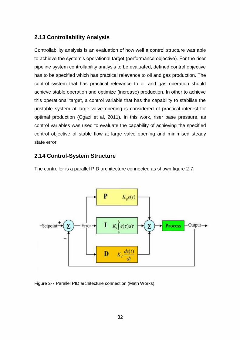
2.13 Controllability Analysis .......................................................................... 32

2.14 Control-System Structure ...................................................................... 32

2.15 Conclusion ............................................................................................ 33

3 MODELLING THE CASE PROBLEM ............................................................ 35

3.1 Building Olga Model for the Numerical Simulation. ................................. 35

3.2 Introduction. ............................................................................................ 35

3.3 Simulation Start Point. ............................................................................ 36

3.4 Pipeline Inlet Flow Rate: ......................................................................... 36

3.5 Pipeline Inlet Condition. .......................................................................... 38

3.6 Pipeline Outlet Condition. ....................................................................... 38

3.7 Burke and Kashou (1996) Pipeline Profile. ............................................. 38

3.8 Basic Olga Model “Texaco”. .................................................................... 41

3.9 Geometry of the Pipeline. ....................................................................... 45

3.10 Fluid Composition. ................................................................................ 45

3.11 Feed Source ......................................................................................... 47

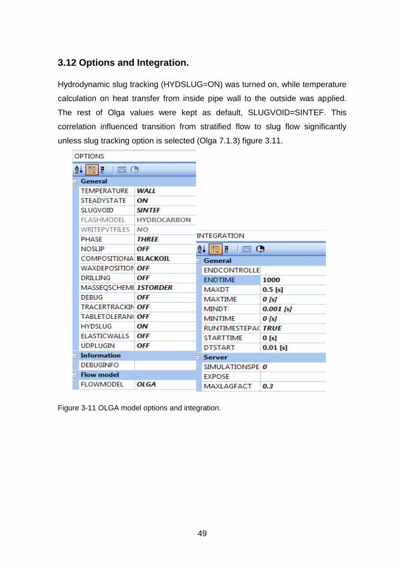
3.12 Options and Integration. ........................................................................ 49

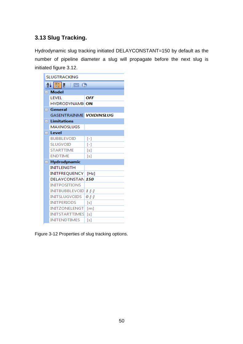
3.13 Slug Tracking. ....................................................................................... 50

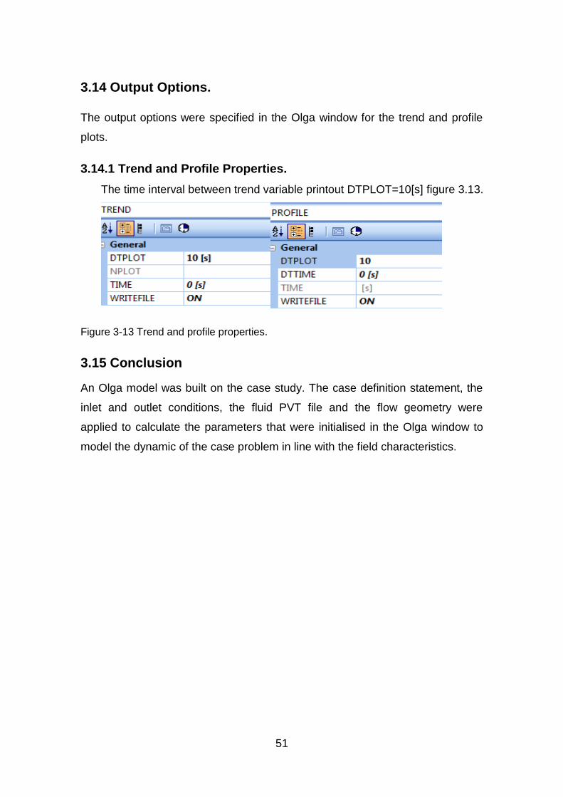
3.14 Output Options. ..................................................................................... 51

3.14.1 Trend and Profile Properties. ......................................................... 51

3.15 Conclusion ............................................................................................ 51

4 SLUG CONTROL DESIGN/TUNING. ............................................................ 53

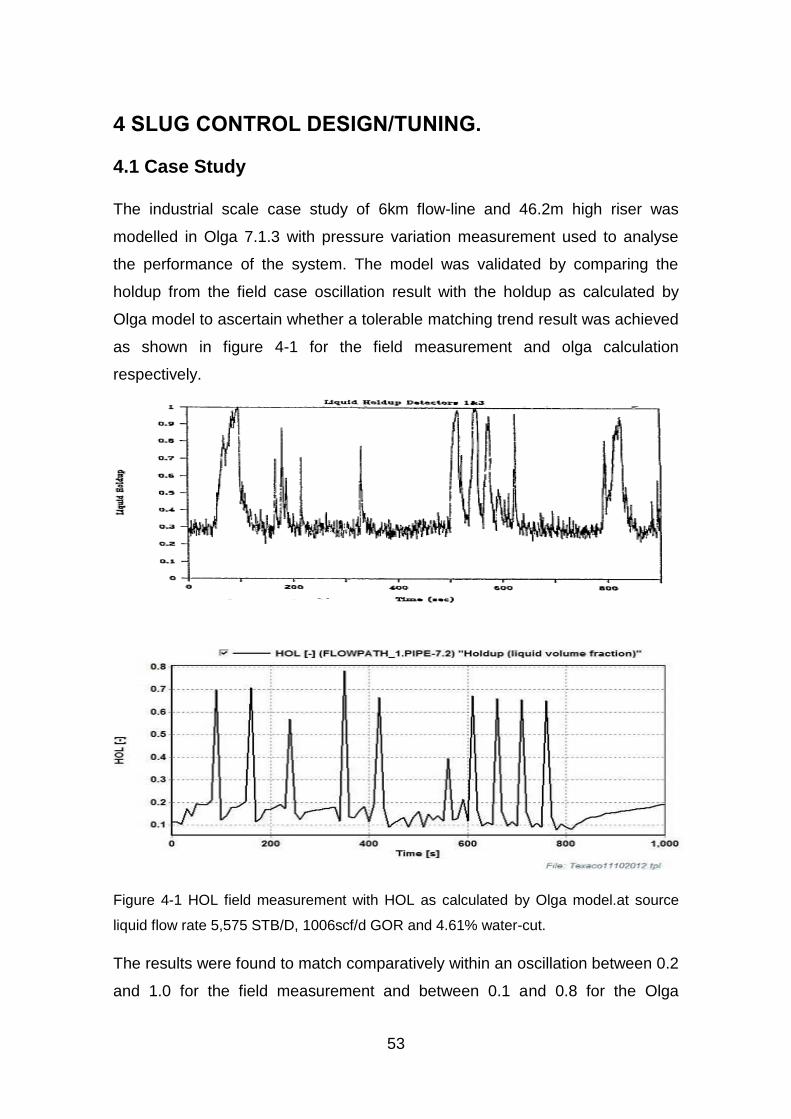
4.1 Case Study ............................................................................................. 53

4.2 Hopf Bifurcation Map .............................................................................. 56

4.3 Controller Design and Tuning ................................................................. 58

4.3.1 Methods for Quantifying the Process Gain ....................................... 58

4.4 Implementing Riser Base Pressure Control ................................... 61

4.5 PID Tuning .............................................................................................. 62

4.5.1 Open-Loop Tuning ........................................................................... 63

4.5.2 PID Tuning Algorithm and GUI ......................................................... 64

4.6 PI Implementation ................................................................................... 64

4.7 Verify if the Design Works ....................................................................... 65

4.8 Results: ................................................................................................... 65

4.9 Achievable Valve Opening to Set-Point Reduction. ................................ 68

4.10 Loss of Stability and Continuous Oscillation. ........................................ 70

4.11 Effect of Automatic Control of Topside Choke Valve Opening .............. 70

5 CONCLUSION / FUTURE WORK ................................................................. 73

5.1 Conclusion .............................................................................................. 73

vii

REFERENCES ................................................................................................. 75

Appendix A Matrices of manual and automatic control ................................. 79

viii

LIST OF FIGURES

Figure 1-1 Hydrodynamic slug propagation (Statoil, 2013) ................................ 3

Figure 1-2 Hydrodynamic slug flow (stratified, wave instability and plugged

hydrodynamic slugging, (Oram, 2013)) ....................................................... 4

Figure 1-3 Hydrodynamic slug flow regimes (Statoil, 2013) ............................... 5

Figure 2-1 Schematic slug fronts in horizontal water-oil-gas flow line (Bratland,

2010) ......................................................................................................... 13

Figure 2-2 Schematics of flow regimes in horizontal pipe (Bratland, 2010). ..... 14

Figure 2-3 Flow regime map for horizontal pipe with gas - liquid two phase flow

(Bratland, 2010). ....................................................................................... 15

Figure 2-4 Schematic of vertical flow regime (Crowe,2009) ............................. 18

Figure 2-5 Flow regime map for vertical pipe with gas–liquid two phase flow

(Bratland, 2010) ........................................................................................ 19

Figure 2-6 Multiphase test facility at Cranfield University (Ogazi et al, 2010) ... 25

Figure 2-7 Parallel PID architecture connection (Math Works). ........................ 32

Figure 3-1 Schematic diagram of pipeline adapted from (Hazem, 2012) with

choke valve at the topside used to analyse the performance of the system

using topside choke valve at liquid source flow rate of 5,575stb/d, GOR

1006 and water-cut 4.61%. ....................................................................... 39

Figure 3-2 Down-comer, flow line and riser profile (Burke and Kashou 1996). 40

Figure 3-3 Properties of carbon steel and poly propylene. ............................... 42

Figure 3-4 Pipeline wall properties. .................................................................. 43

Figure 3-5 Schematic diagram of OLGA model with the nodes and source inlet.

.................................................................................................................. 44

Figure 3-6 Node properties. ............................................................................. 44

Figure 3-7 Geometry of the pipeline model Burke and Kashou 1996. .............. 45

Figure 3-8 Properties of black oil components. ................................................ 46

Figure 3-9 Properties of the black oil feed. ....................................................... 47

Figure 3-10 Source properties. ......................................................................... 48

Figure 3-11 OLGA model options and integration. ........................................... 49

Figure 3-12 Properties of slug tracking options. ............................................... 50

ix

Figure 3-13 Trend and profile properties. ......................................................... 51

Figure 4-1 HOL field measurement with HOL as calculated by OLGA model.at

source liquid flow rate 5,575 STB/D, 1006scf/d GOR and 4.61% water-cut.

.................................................................................................................. 53

x

LIST OF TABLES

Table 3-1 Burke and Kashou (1996) fluid PVT composition. .... Error! Bookmark

not defined.

Table 3-2 Burke and Kashou (1996) Pipeline Details. ..................................... 41

Table 3-3 Detail of pipeline geometry. .............................................................. 45

Table 4-1 Ziegler-Nichols open-loop tuning rule. .............................................. 60

Table 4-2 PI tuning parameters. ....................................................................... 63

Table 4-3 Process and controller parameters .................................................. 71

xi

LIST OF NOMENCLATURES

Area occupied by gas (m2)

Area occupied by liquid (m2)

Cross sectional area of the pipe (m2)

Drag coefficient

Pipe inner diameter (m)

ƒ Darcy-Weisbach friction factor

𝑔 Acceleration due to gravity (m/s2)

Liquid height in the pipe(m)

Length of vertical pipe (m)

Volumetric gas flow rate (m3/s)

Volumetric liquid flow rate (m3/s)

Volumetric oil flow rate (m3/s)

Volumetric water flow rate (m3/s)

Length of surface contact between gas and liquid in pipe

cross-section (m)

Gas velocity (m/s)

Gas velocity transition from stratified wavy flow to annular

flow(m/s)

Gas velocity transition from stratified flow to stratified wavy

flow(m/s)

Liquid velocity (m/s)

Liquid velocity transition from slug flow to dispersed bubble

flow(m/s)

Velocity of the mixture (m/s)

Superficial gas velocity (m/s)

xii

Superficial liquid velocity (m/s)

Critical droplet Weber number, between 20 or 30

Liquid volume fraction or liquid fraction

Gas volume fraction or gas fraction

Energy dissipated per unit mass (m2/s3)

Dynamic viscosity of liquid (kg/m.s)

Angle of inclination of the pipe ( for horizontal pipe

Liquid density (kg/m3)

Gas density (kg/m3)

Surface tension between liquid and gas (N/m)

Production rate

Production index

Pressure of the reservoir (bara)

Flow line pressure (bara)

Riser base pressure (bara)

Average riser base pressure over time T (bara)

Total production over time T (STB/D)

Maximum pressure (bara)

Minimum pressure (bara)

Production period (s)

Slug period (s)

Number of segments

Starting time (s)

OLGA OiLGAs

1

1 INTRODUCTION

1.1 Background

The ever increasing population and urbanization with its attendant high demand

for energy, coupled with increase in oil prices since 1970s, has necessitated

extensive research on finding new technology that can increase oil production

and recovery from different fields. Today many oil wells are produced at satellite

fields/hostile offshore environment where the productions from several wells are

transported via manifolds in tie-in long distant pipeline from seabed to the

receiving process facility. In this regard, a mixture of gas, oil, water and

sometimes sand, hydrates, asphaltenes and wax are transported through

distant pipelines to the platform for processing. The flow assurance challenges

covers an entire spectrum of design tools, methods, equipment, knowledge and

professional skills needed to ensure the safe, uninterrupted and simultaneous

transport of gas, oil and water from reservoirs to the processing facility

(Storkaas,2005). The cost of processing offshore is enormous in terms of

Capital Expenditure (CAPEX) and Operation Expenditure (OPEX) due to

technical difficulties of producing offshore, and considering the limited space

available and other consideration such as harsh weather.

Slug flow that arises in multiphase (gas, oil, water) transport is a major

challenge in oil exploration, production, recovery and transport. Slugging is the

intermittent flow regime in which large bubbles of gas flow alternately with liquid

slugs at randomly fluctuating frequency (Issa and Kempf, 2003) in pipeline. Slug

causes a lot of problems due to rapid changes in gas and liquid rate entering

the separators and the large variations in system pressure. Slug flow is a

regular phenomenon in many engineering applications such as the transport of

hydrocarbon fluids in pipelines, liquid-vapour flow in power plants and

buoyancy-driven equipment (Fabre and Line’, 1992). The slug can be formed in

low-points in the topography of the pipeline. It can be hydrodynamic induced

slugging, terrain induced slugging or operation induced slugging.

2

Hydrodynamic slugging, which is the main subject of this project occur in a

horizontal or near horizontal pipes and can be generated by two main

mechanisms (i) natural growth of hydrocarbon instability and (ii) liquid

accumulation due to instantaneous imbalance between pressure and

gravitational forces caused by pipe undulations (Issa and Kempf, 2003) .

For the natural growth phenomenon, small random perturbation of short

wavelengths arising naturally may grow into larger and longer waves on the

surface of the liquid due to the Kelvin-Helmholtz instability (Ansari, 1998).

These waves may continue to grow as it transverses the length of the pipe line,

picking up liquid flowing ahead of them, until they bridge the pipe cross-section,

thereby forming slug. In real flow, all these events take place at different times,

hence some slugs grow, while others collapse and they may travel at different

speeds leading to the merging of some slugs with others (Taitel and Barnea,

1990).

In the case of liquid accumulation, slug flow may form at pipe dips due to the

retardation and subsequent accumulation of liquid in the dips leading to the

filling up of the cross-section with liquid. This is an extreme example of terrain

induced slug flow also called “severe slugging” and occurs when a slightly

inclined pipeline meets a vertical riser (Schmidt et at, 1985; Jansen et al, 1996).

Slug may arise by the combination of the mentioned mechanisms

simultaneously in long hydrocarbon transport pipelines. In such cases, the slugs

generated from one mechanism interact with those arising from the second

leading to a complex pattern of slugs, which may overtake and combine (Issa

and Kempf, 2003).

The intermittency of slug flow causes severe unsteady loading on the pipelines

carrying fluid as well as on the receiving facility such as the separators. This

gives rise to problems in design and therefore it is important to be able to

predict the onset and subsequent development of slug flow and its control.

The purpose of this work was to investigate the capability of active feedback

control strategy based on measurement of pressure or holdup transmitter at the

3

riser base as controlled variable with topside choking as manipulated variable

with PI controller in Olga simulation to mitigate hydrodynamic slug flow.

1.2 Hydrodynamic Slugging

Hydrodynamic slug is initiated by the instability of waves on the gas /liquid

interface in stratified flow. The gas /liquid interface is lifted to the top of the pipe

when the velocity difference between gas phase and liquid phase is high

enough. This wave growth is triggered by the Kelvin-Helmholtz instability and

when the wave reaches the top of the pipe, it forms slug blocking the gas

passage in the flow line see figures 1-1, 1-2, 1-3 and 1-4 respectively. At this

point the liquid volume fraction (holdup) is one as the gas volume fraction tends

to zero. When the slug front travels faster than the slug tail, the slug grows.

Conversely, if the slug tail travels faster than the slug front, the slug decays. If

the slug front and the slug tail travel at the same speed, a stable slug is

obtained. When the gas velocity is high enough, gas will be entrained in the

liquid as gas entrainment figure 1-1.

Figure 1-1 Hydrodynamic slug propagation (Varne, V. 2010)

4

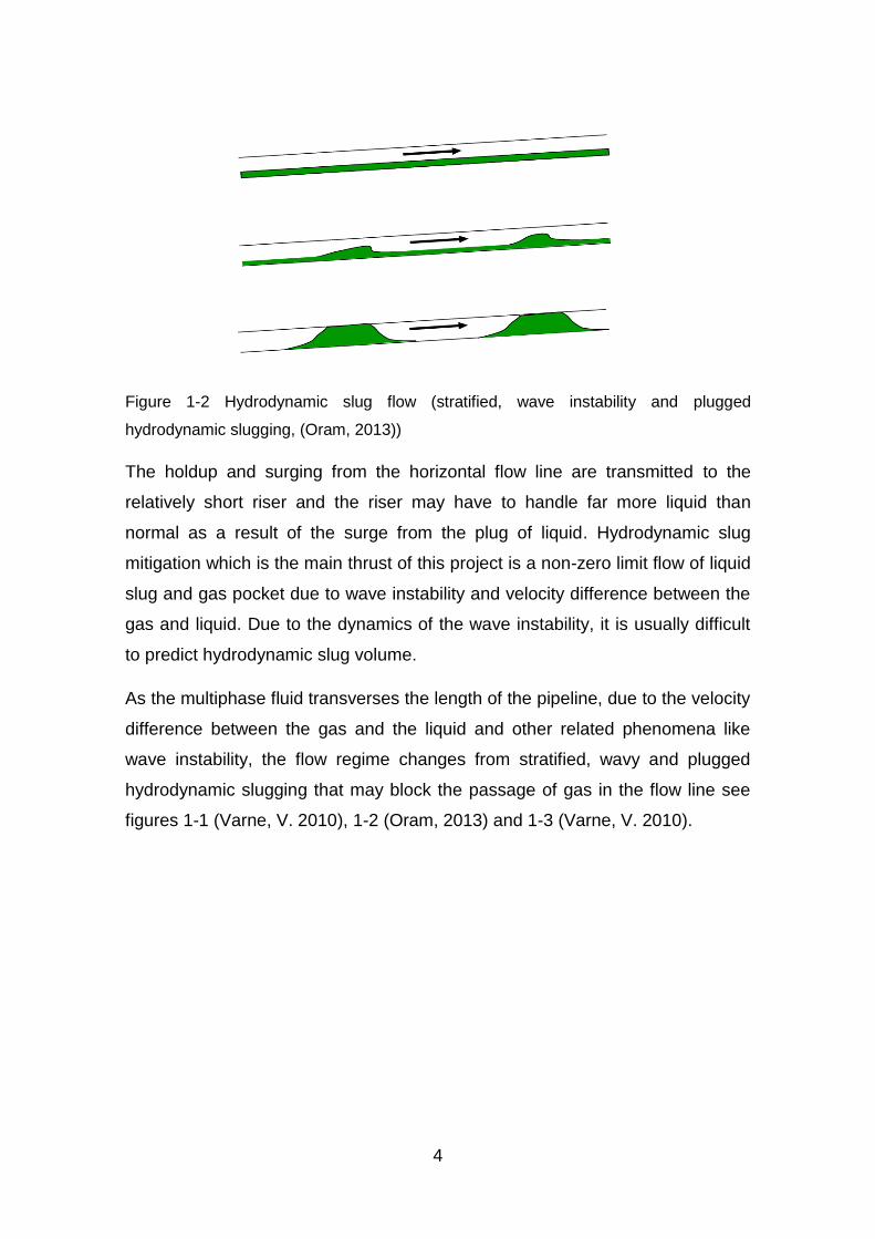
Figure 1-2 Hydrodynamic slug flow (stratified, wave instability and plugged

hydrodynamic slugging, (Oram, 2013))

The holdup and surging from the horizontal flow line are transmitted to the

relatively short riser and the riser may have to handle far more liquid than

normal as a result of the surge from the plug of liquid. Hydrodynamic slug

mitigation which is the main thrust of this project is a non-zero limit flow of liquid

slug and gas pocket due to wave instability and velocity difference between the

gas and liquid. Due to the dynamics of the wave instability, it is usually difficult

to predict hydrodynamic slug volume.

As the multiphase fluid transverses the length of the pipeline, due to the velocity

difference between the gas and the liquid and other related phenomena like

wave instability, the flow regime changes from stratified, wavy and plugged

hydrodynamic slugging that may block the passage of gas in the flow line see

figures 1-1 (Varne, V. 2010), 1-2 (Oram, 2013) and 1-3 (Varne, V. 2010).

5

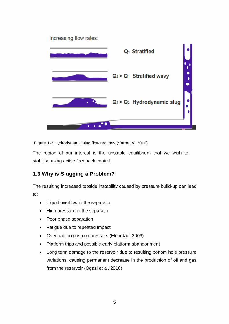
Figure 1-3 Hydrodynamic slug flow regimes (Varne, V. 2010)

The region of our interest is the unstable equilibrium that we wish to

stabilise using active feedback control.

1.3 Why is Slugging a Problem?

The resulting increased topside instability caused by pressure build-up can lead

to:

Liquid overflow in the separator

High pressure in the separator

Poor phase separation

Fatigue due to repeated impact

Overload on gas compressors (Mehrdad, 2006)

Platform trips and possible early platform abandonment

Long term damage to the reservoir due to resulting bottom hole pressure

variations, causing permanent decrease in the production of oil and gas

from the reservoir (Ogazi et al, 2010)

6

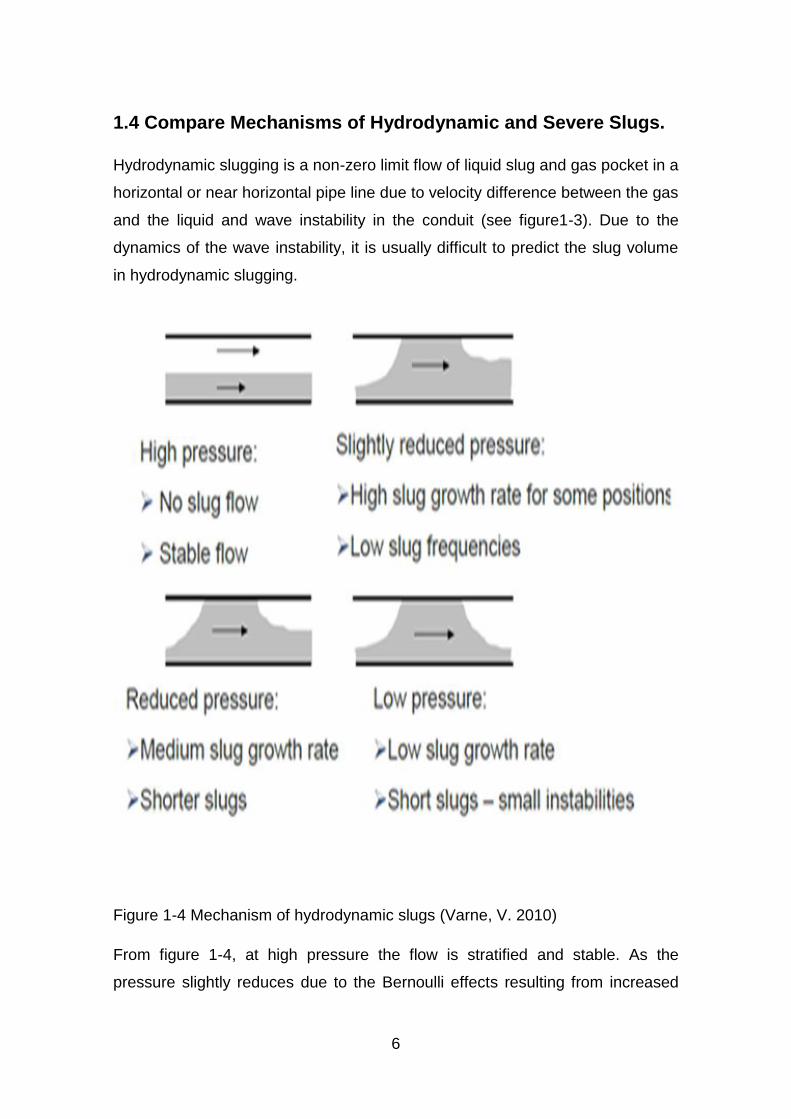
1.4 Compare Mechanisms of Hydrodynamic and Severe Slugs.

Hydrodynamic slugging is a non-zero limit flow of liquid slug and gas pocket in a

horizontal or near horizontal pipe line due to velocity difference between the gas

and the liquid and wave instability in the conduit (see figure1-3). Due to the

dynamics of the wave instability, it is usually difficult to predict the slug volume

in hydrodynamic slugging.

Figure 1-4 Mechanism of hydrodynamic slugs (Varne, V. 2010)

From figure 1-4, at high pressure the flow is stratified and stable. As the

pressure slightly reduces due to the Bernoulli effects resulting from increased

7

gas velocity, a wave build-up is initiated in the flow line that can grow to fill the

pipe diameter and hence block the gas flow in the pipeline.

Severe slugging or terrain induced slugging in the other hand may occur at low

flow rates, when a downwards incline or horizontal pipeline is connected to a

vertical riser. It is characterized by a cyclic behaviour alternating between no

liquid flows at the outlet, to a high liquid delivery (surge) at the outlet. These

occur when the rate of liquid flow to the riser is higher than the rate of flow up

the riser and thus can cause an accumulation. The maximum slug volume in

severe slugging is usually the height of the riser. This slug type is cyclic and

characterized by blockage of flow at the dip or low points resulting in pressure

build-up upstream the blockage until the compressed gas upstream is able to

overcome the gravitational head, causing a blowout of liquid.

8

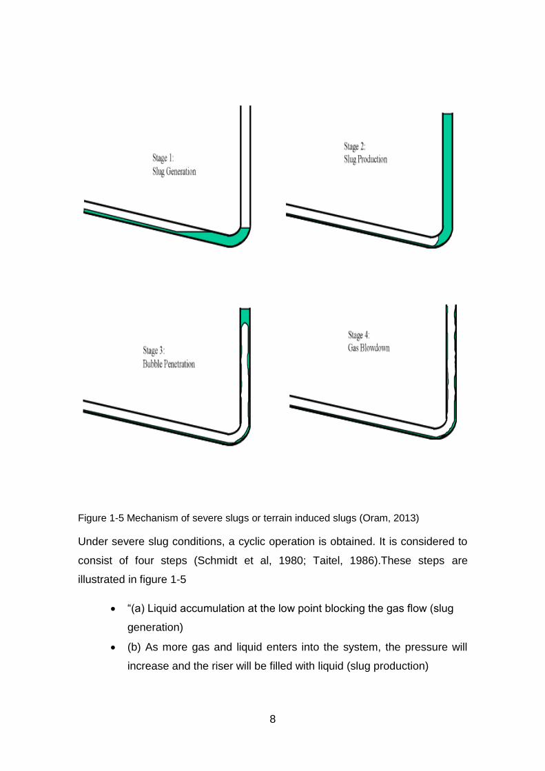
Figure 1-5 Mechanism of severe slugs or terrain induced slugs (Oram, 2013)

Under severe slug conditions, a cyclic operation is obtained. It is considered to

consist of four steps (Schmidt et al, 1980; Taitel, 1986).These steps are

illustrated in figure 1-5

“(a) Liquid accumulation at the low point blocking the gas flow (slug

generation)

(b) As more gas and liquid enters into the system, the pressure will

increase and the riser will be filled with liquid (slug production)

9

(c) After a while the amount of gas that is blocked will be large

enough to blow the liquid out as gas penetrates into the riser (bubble

penetration)

(e) After the blowout, the pressure drops and fluid falls back for a new

slug cycle to start to form (slug blowout).”

1.5 Operation Induced Slugging

This type of slug could be induced by operational changes in the system, such

as start-up, ramp-up, or pigging etc. During start-up, slug may be formed owing

to liquid which settled at the low points in the line after shutdown. Also when

there is a change in the steady condition of flow (flow rate change) in the

multiphase flow line. For example, when there is a production rate drop or

increase for a line operating in stratified flow, slug could be formed. Transient

simulator Olga can be used to simulate such a condition.

Most of the earlier works on slug mitigation (Yocum, 1973, Schmidt et al, 1980),

concentrated on the mitigation of the flow instability with little emphasis on the

effect of the mitigation strategy on oil production and recovery. These limitations

propelled a continued research on slug control strategies to investigate further

into methods that will enhance optimal production and recovery. Recently,

(Ogazi, et at, 2009), reported the effectiveness of feedback control as severe

slug mitigation strategy with a robust controller, while the current work seek to

extend investigation on the effectiveness of feedback control strategy to

mitigate hydrodynamic slugging.

1.6 Slug Mitigation and Prevention Methods

There are a number of slug mitigation and prevention methods, which includes:

“Increasing the flow rate

Riser base gas injection

Gas lift in the well

Fixed topside choking

Combination of gas injection and topside choking

10

Slug catcher

Active feedback control

Modified flow line layout/riser base geometry to avoid a dip”(Yocum,

1973)

This research project utilized topside choking to control hydrodynamic slug

flow problem with active feedback.

1.7 Aim.

The aim of this research is to develop a method for hydrodynamic

slug control using topside choking with active feedback control.

To achieve this aim, the following objectives were pursued.

1.8 Objectives.

Investigate the suitability of active feedback control using topside

choke for hydrodynamic slug control.

Perform controllability analysis on the possible control variables.

Investigate the effectiveness of this control strategy to improve oil

production and recovery

1.9 Conclusion

Hydrodynamic slugs have been found to occur in a horizontal or near horizontal

pipeline by two main mechanisms (i) natural growth of hydrocarbon instability

due to Kelvin-Helmholtz instability (ii) liquid accumulation due to instantaneous

imbalance between pressure and gravitational forces caused by pipe

undulations. Slug may also arise by the combination of the two mechanisms

presented simultaneously in long hydrocarbon transport pipeline. In such case,

the slug generated from one mechanism interacts with those arising from the

second mechanism leading to a complex pattern of slugs which may overtake

and combine. The slug may grow when the slug front travels faster than the

slug tail or travelling an upward inclination. It may decay when the slug tail

travels faster than the slug front or travelling a downward inclination. If both the

11

slug front and the slug tail travel at the same speed, a stable slug may be

formed.

Active feedback control technology has not been extended for the investigation

of hydrodynamic slug control in the literature. This extension of the capability of

active feedback control technology with topside choke valve to mitigate

hydrodynamic slug flow is the main contribution of the present work.

13

2 LITERATURE REVIEW

2.1 Multiphase Flow

Multiphase flow is a very complex flow behavior and its description depends

heavily on the flow regime detection. To be able to calculate important factors

such as pressure drop and flow rates, it is critical to know the flow regime in all

parts of the system.

The parameters that determine which flow regime will occur is also changing

with time as the wells are getting more and more depleted at the end of their

life-time. This means that the engineers must plan for different scenarios when

designing the production and process system.

Slugging is a flow regime that causes a lot of problems due to rapid changes in

gas and liquid rates entering the separators and large variations in system

pressure. It can be hydrodynamic slugging, terrain induced slugging or

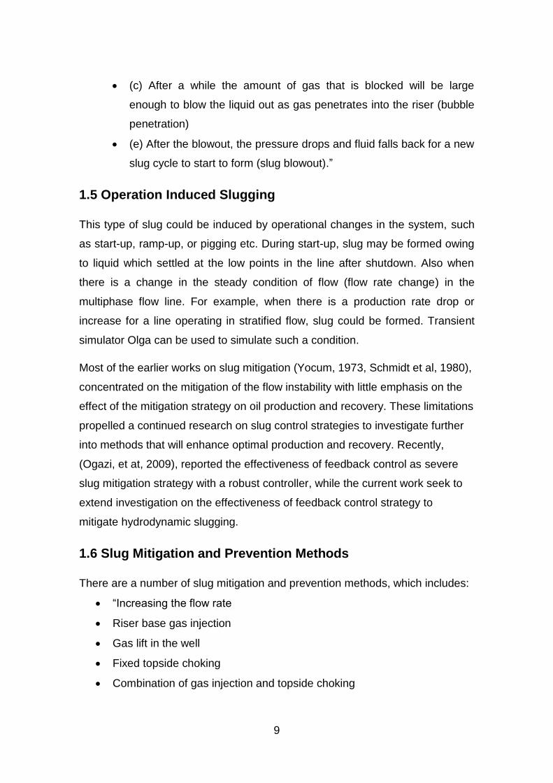
operation induced slugging. Figure 2-1 show three phases water, oil and gas as

they transverse a horizontal pipe cross-section.

Figure 2-1 Schematic slug fronts in horizontal water-oil-gas flow line (Bratland, 2010)

The understanding of how water, oil and gas in a conduit respond to pressure

changes, flow rate changes, composition, density changes, viscosity changes,

and temperature changes etc, will help the operator to predict accurately the

development of transient flows usually caused by slug propagation. Traditional

flow pattern has been produced as a tool to predict the flow regime that will

develop in the pipeline (Taitel and Dukler, 1976; Barnea, 1977).

Water

Oil

Gas

14

2.2 Flow Regime Determination

Determining flow regime is critical in the analysis of multiphase flow. In cases

where the flow happens to be near the border between two or even three

different flow regimes, the uncertainties are generally most significant. We may

also experience situations where minor changes in flow properties or inclination

angle is likely to change the flow regime, and simulation may require more

accurate pipe elevation profile or fluid composition data than are available.

These uncertainties are investigated by simulating several times with slightly

different input-data to see how the results compare. The main mechanism at

work in the switching from one flow regime to another is thought to be the

Bernoulli effects, which reduces the pressure if the gas velocity is increased

(Bratland, 2010).

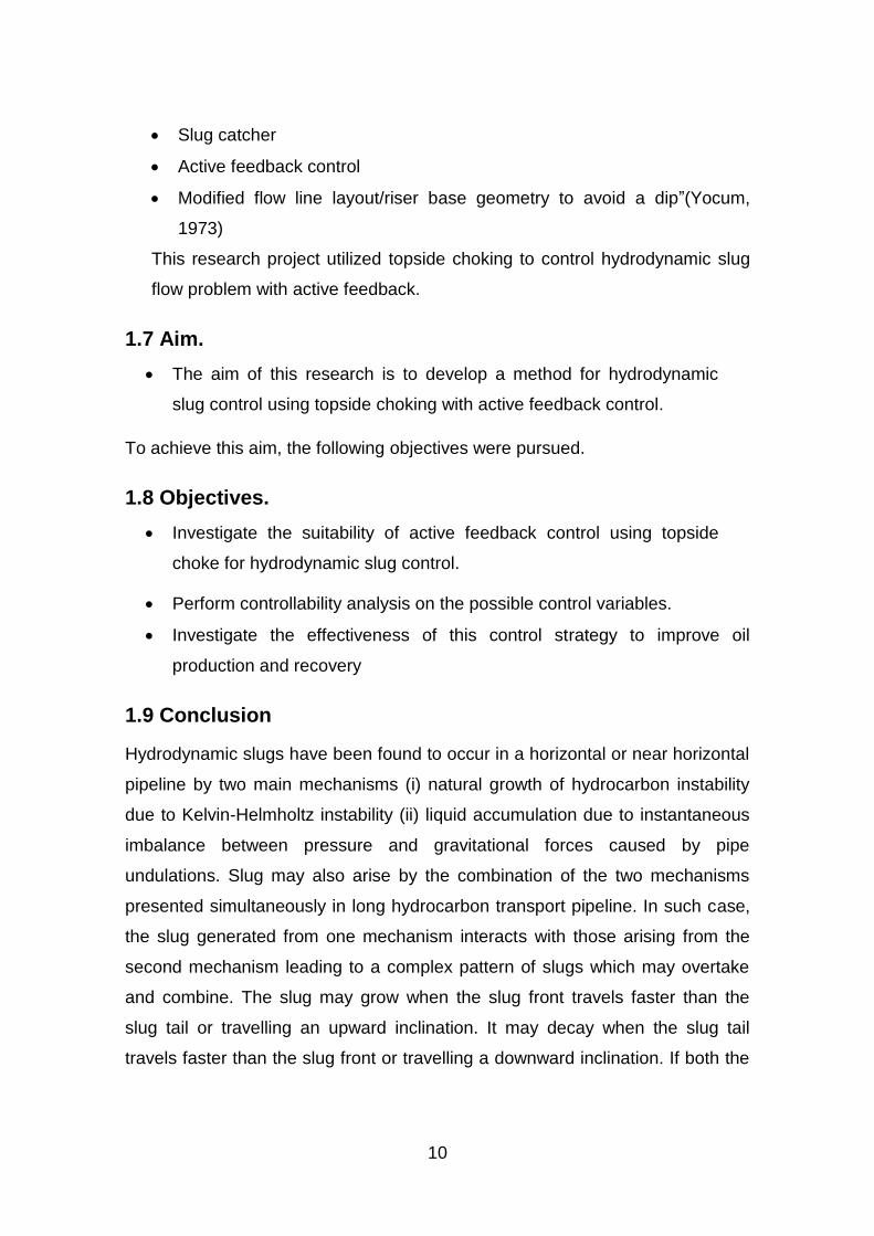
2.2.1 Flow Regime Map in Horizontal Pipe

Figure 2-2 shows the flow regimes that may develop as the multiphase fluid

flows across the pipeline at varying conditions.

Figure 2-2 Schematics of flow regimes in horizontal pipe (Bratland, 2010).

15

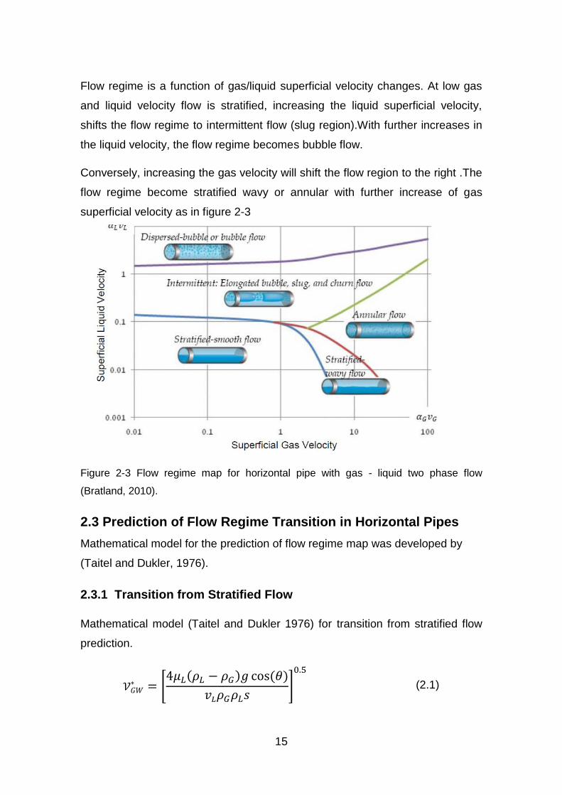
Flow regime is a function of gas/liquid superficial velocity changes. At low gas

and liquid velocity flow is stratified, increasing the liquid superficial velocity,

shifts the flow regime to intermittent flow (slug region).With further increases in

the liquid velocity, the flow regime becomes bubble flow.

Conversely, increasing the gas velocity will shift the flow region to the right .The

flow regime become stratified wavy or annular with further increase of gas

superficial velocity as in figure 2-3

Figure 2-3 Flow regime map for horizontal pipe with gas - liquid two phase flow

(Bratland, 2010).

2.3 Prediction of Flow Regime Transition in Horizontal Pipes

Mathematical model for the prediction of flow regime map was developed by

(Taitel and Dukler, 1976).

2.3.1 Transition from Stratified Flow

Mathematical model (Taitel and Dukler 1976) for transition from stratified flow

prediction.

[

( 𝑔 (

]

(2.1)

16

Dynamic viscosity of liquid [kg/m.s]

Liquid density [kg/m3]

Gas density [kg/m3]

𝑔 Acceleration due to gravity [m/s2]

Angle of inclination of the pipe [ , for horizontal pipe

S Sheltering coefficient 0.01

Liquid velocity [m/s]

Gas velocity [m/s]

When the gas velocity is greater than the flow regime will change from

stratified flow to stratified wavy flow (blue line of figure 2-3). These flow regimes

are assumed accurate within the limit of angle of inclination (Bratland,

2010)

2.3.2 Transition to Annular Flow

Bratland, (2010) reported that Bernoulli principle was applied by Taitel and

Duckler to predict transition to annular flow.

(

) [

( (

]

(2.2)

Liquid height in the pipe [m]

𝑑 Pipe inner diameter [m]

Gas velocity transition from stratified wavy to annular flow (m/s)

Length of surface contact between gas and liquid in pipe cross-

section[m]

AG Cross–sectional area of the gas [m2]

𝑔 Acceleration due to gravity [m/s2]

17

Flow becomes annular when the gas velocity exceeds

(red line of figure 2-

3)

Taitel et al, (1980) found that liquid height in the pipe has to be less than

0.35 of internal diameter for the flow to be in annular flow, otherwise the flow

would be slug flow. This is summarized in the following conditions (Bratland,

2010)

Annular flow if and 𝑑 (2.3)

Slug flow if and 𝑑 (2.4)

2.3.3 Transition to Dispersed Bubble Flow

When the liquid velocity is further increased, the flow become turbulent which

leads to crushing the Taylor bubbles to small dispersed bubble (Bratland,

2010).The flow transits from slug flow to dispersed bubble flow (grey line of

figure 2-3) represented by the equation 2.5 (Bratland, 2010)

[

(

( –

)]

(2.5)

ƒ Darcy-Weisbach friction factor

Transition velocity from slug flow to Dispersed bubble flow. When the

liquid velocity exceed the flow becomes dispersed bubble flow.

2.4 Flow Regime in Vertical Pipes

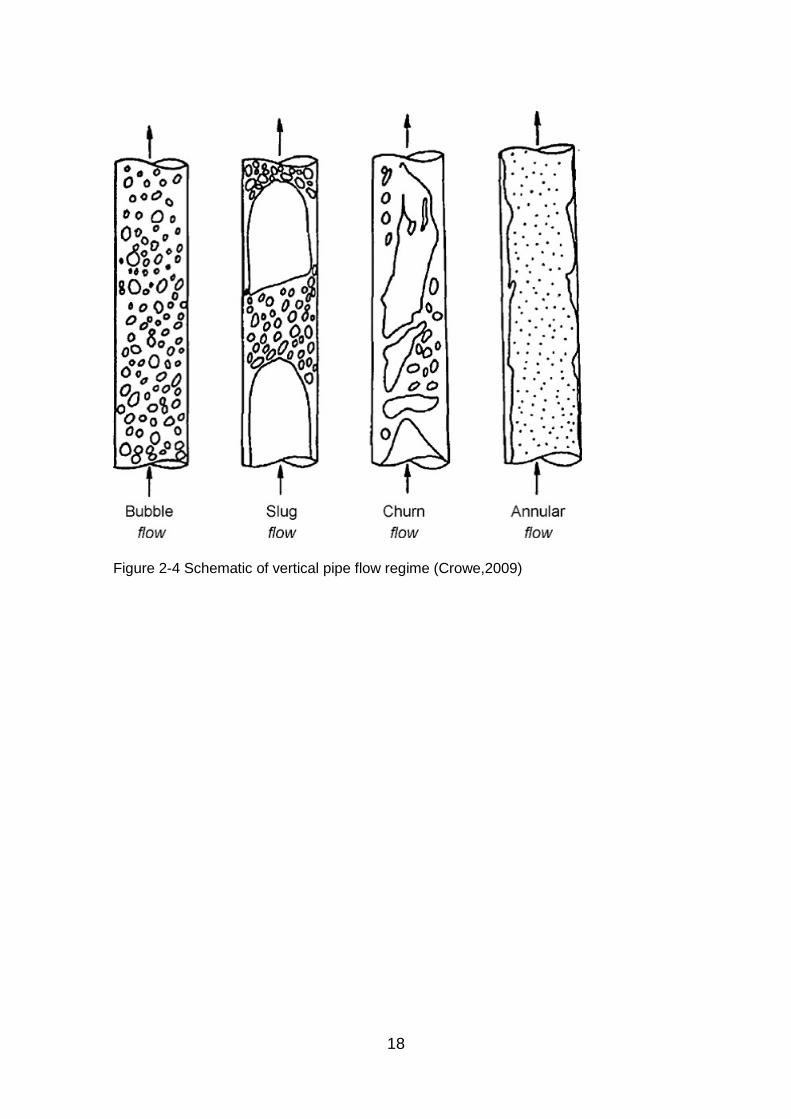
It is highly dependent on the in-coming gas flow rate, as the amount of gas is

gradually increased, the flow regime transit from bubble flow, slug (intermittent)

flow, churn flow, and annular flow respectively in vertical pipes. For annular flow

the liquid film at the wall no longer have a uniform thickness. Figure 2-4 shows

the flow regime transition that may occur in vertical pipes.

18

Figure 2-4 Schematic of vertical pipe flow regime (Crowe,2009)

19

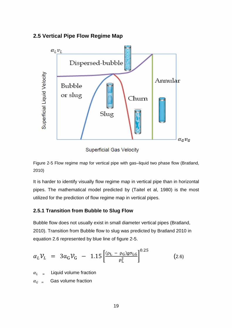
2.5 Vertical Pipe Flow Regime Map

Figure 2-5 Flow regime map for vertical pipe with gas–liquid two phase flow (Bratland,

2010)

It is harder to identify visually flow regime map in vertical pipe than in horizontal

pipes. The mathematical model predicted by (Taitel et al, 1980) is the most

utilized for the prediction of flow regime map in vertical pipes.

2.5.1 Transition from Bubble to Slug Flow

Bubble flow does not usually exist in small diameter vertical pipes (Bratland,

2010). Transition from Bubble flow to slug was predicted by Bratland 2010 in

equation 2.6 represented by blue line of figure 2-5.

[(

]

(2.6)

iquid volume fraction

Gas volume fraction

20

Liquid velocity [m/s]

Gas velocity [m/s]

Surface tension between gas and liquid [N/m]

𝑔 Acceleration due to gravity [m/s2]

2.5.2 Transition to Dispersed Bubble Flow

When the liquid velocity is high enough, bubble flow transition occurs, and the

turbulent flow mixes the bubbles with the liquid (grey line) of figure 2-5

(Bratland, 2010)

( √

) [

( ]

(2.7)

2.5.3 Transition from Slug to Churn Flow

Churn flow occurs when the gas flow rate increase until the slug length decays

to zero. Choham, (2006) reported that flow regime at inlet of a vertical pipe is

always churn flow and the flow regime changes to slug as distance into the pipe

increase. Bratland, (2010) described the transition by the equation 2.8

represented by the (red line) of figure 2-5.

(

√ (2.8)

Length of the vertical pipe [m]

2.5.4 Transition from Churn to Annular Flow

When the gas flow rate is further increased, the flow regime changes from

churn flow to annular flow as presented by the (green line) in figure 2-5

(Bratland, 2010) in equation 2.9.

[

(

]

(2.9)

21

Critical droplet Weber number, between 20 or 30

Drag coefficient CD is obtained by iteration.

2.6 Terminology Used in Multiphase Flow Literature

This section defines some of the terminology used in the thesis as obtained

from multiphase flow literature (Handbook of Multiphase Flow Metering, 2005).

2.6.1 Volume Fraction and Holdup

This is the area occupied by one phase in the cross sectional area of the

pipeline (Bratland, 2010). If the area fraction is occupied by the liquid, it is

termed liquid area fraction or holdup. Since volume corresponds to area if the

length of that volume is infinitely small (infinitely small pipe length), this area can

be termed volume fraction for the liquid or gas respectively.

⁄ and

⁄ (2.10)

Liquid volume fraction or liquid fraction

Gas volume fraction or gas fraction.

Area occupied by gas [m2]

Area occupied by liquid [m2]

A Area of pipe cross-section [m2]

2.6.2 Superficial Velocity

The average fluid velocity in one phase is calculated by dividing the volume flow

rate by the pipe cross-sectional area, as average fluid speed is difficult to

calculate in multiphase flow. The assumption of single phase is made as

running solely in the pipe to calculate the superficial velocity thus:

⁄ and

⁄ (2.11)

22

Superficial liquid velocity [m/s]

Superficial gas velocity [m/s]

Volumetric liquid flow rate [m3/s]

Volumetric gas flow rate [m3/s]

⁄ and

⁄ (2.12)

Where

Gas velocity [m/s]

Liquid velocity [m/s]

2.6.3 Water-Cut

The ratio between the volumetric flow rates of water to the total volumetric flow

rate of liquid (used in oil extraction when water is produced as part of well

production).

Water-cut

⁄ (2.13)

= volumetric water flow rate [m3/s]

2.6.4 Gas Oil Ratio (GOR)

Gas-Oil ratio is the ratio between produced volumetric flow rate of gas to the

volumetric flow rate of oil when oil and gas are produced as part of well

production.

GOR

⁄ (2.14)

Volumetric oil flow rate [m3/s]

23

2.6.5 Gas Liquid Ratio (GLR)

Ratio between produced volumetric gas flow rate to the volumetric flow rate of

total liquid viz (oil plus water)

GLR = QG/QL (2.15)

2.7 Standard Condition

Standard conditions are internationally accepted reference measurement

applied in the oil industry. The standard conditions as defined per British

Standard (British Standard, 2005) at temperature 288.15k (15◦C or 59F).

However, imperial units referred to as field units are commonly applied by the

oil industries. This imperial/field unit is applied by Olga calculation with in-built

metric units. Examples of such field units are Million Standard Cubic Feet per

Day (MMscf/d) for gas volumetric flow rate and Standard Barrel per Day

(STB/d) for oil.

2.8 Review of slug control techniques

In other to effectively deal with the hydrodynamic slug problems, a number of

publications review on the earlier works were investigated to gain insight into

the progress made in this area.

The earlier work on slug control reported in literature was (Yocum, 1973), which

concentrated on flow stability with little emphases on effect on production.

The publication identified several slug elimination techniques that are still

referenced till today. These techniques include reduction in the pipeline

diameter; splitting of the flow into multiple streams; gas injection into the riser or

a combination of gas injection and choking. Yocum reported that increased

back-pressure could eliminate slugging but would severely reduce the flow

capacity up to 60%. Contrary to Yocum’s report, Schmidt et al,(1985) noted that

slugging in a pipeline riser system could be eliminated or minimized by choking

at the riser top with little or no change in the flow rates and pipeline pressure.

24

Schmidt also indicated that elimination of slugging could be achieved by gas

injection, but dismissed it as not being economically viable due to the cost of a

compressor to pressurize the gas for injection and piping required to transport

the gas to the base of the riser.

Hills, (1990) described riser base gas injection test performed on the S.E.

Forties field to eliminate slugging. The gas injection was shown to reduce the

extent of slugging. The condition for eliminating slugging using gas injection

was to bring the flow regime in the riser to annular flow thus preventing liquid

accumulation at the riser base.

Jansen (1990) investigated different elimination techniques such a back-

pressure increase, choking, gas injection, choking and gas injection

combination. He made the following observations:

“Very high back-pressures were required to eliminate severe slugging. Careful

choking was needed to stabilize the flow with minimal back-pressure increase.

Large amounts of gas were needed to stabilize the flow with gas injection

method only” (Jansen 1990).

Choking and gas injection combination are being considered as a viable method

for slug control, reducing the degree of choking and the amount of gas injection

needed to stabilize the flow and yield an optimal production.

Jansen and Shoham (1994), worked together on mitigation of terrain induced

slug using combination of advantages of choking and gas injection. The idea

was to combine the advantages of both methods; increased choke valve

opening, plus reduced gas injection rate as a viable approach to stabilized

controlled start-up of a smooth flow system.

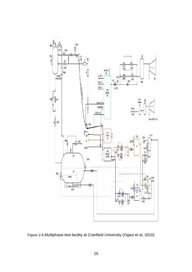
Ogazi et al, (2010) studied severe slug control with maximal choke valve

opening with a robust PID controller using the Cranfield University multiphase

test facility to maximize oil production.

25

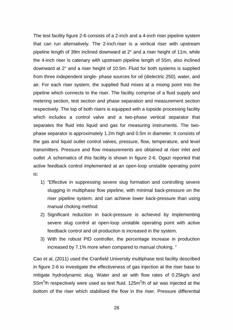
Figure 2-6 Multiphase test facility at Cranfield University (Ogazi et al, 2010)

26

The test facility figure 2-6 consists of a 2-inch and a 4-inch riser pipeline system

that can run alternatively. The 2-inch.riser is a vertical riser with upstream

pipeline length of 39m inclined downward at 2 and a riser height of 11m, while

the 4-inch riser is catenary with upstream pipeline length of 55m, also inclined

downward at 2 and a riser height of 10.5m. Fluid for both systems is supplied

from three independent single- phase sources for oil (dielectric 250), water, and

air. For each riser system, the supplied fluid mixes at a mixing point into the

pipeline which connects to the riser. The facility comprise of a fluid supply and

metering section, test section and phase separation and measurement section

respectively. The top of both risers is equipped with a topside processing facility

which includes a control valve and a two-phase vertical separator that

separates the fluid into liquid and gas for measuring instruments. The two-

phase separator is approximately 1.2m high and 0.5m in diameter. It consists of

the gas and liquid outlet control valves, pressure, flow, temperature, and level

transmitters. Pressure and flow measurements are obtained at riser inlet and

outlet .A schematics of this facility is shown in figure 2-6. Ogazi reported that

active feedback control implemented at an open-loop unstable operating point

is:

1) “Effective in suppressing severe slug formation and controlling severe

slugging in multiphase flow pipeline, with minimal back-pressure on the

riser pipeline system, and can achieve lower back-pressure than using

manual choking method.

2) Significant reduction in back-pressure is achieved by implementing

severe slug control at open-loop unstable operating point with active

feedback control and oil production is increased in the system.

3) With the robust PID controller, the percentage increase in production

increased by 7.1% more when compared to manual choking. “

Cao et al, (2011) used the Cranfield University multiphase test facility described

in figure 2-6 to investigate the effectiveness of gas injection at the riser base to

mitigate hydrodynamic slug. Water and air with flow rates of 0.25kg/s and

5Sm3/h respectively were used as test fluid. 125m3/h of air was injected at the

bottom of the riser which stabilised the flow in the riser. Pressure differential

27

across the riser was used as controlled variable to control the opening of the

gas injection valve and 4.19% reduction in gas injection rate was reported as

achieved with active control. The present work seeks to investigate the

effectiveness of active feedback control using the topside choke valve to

mitigate hydrodynamic slug flow.

2.9 Control and Controllability Analysis

The primary objective of process control is to maintain a process at a desired

operating conditions, safely and efficiently, while satisfying environmental and

product quality requirements (Seborg et al, 2004). In feedback control system,

the controller looks at the actual measured output and compares it with the

desired value (set-point), and returns a corrective action when there is deviation

(error) between the set-point and the measured output as may be appropriate.

The three important process variables are:

“Controlled variable (CV): These are process variables that are

controlled, and the desired values of a controlled variable is referred to

as its set-point

Manipulated variable (MV): The process variables that can be adjusted in

order to keep the controlled variables at or near the set-point.

Disturbance variable (DV): These are process variables that affect the

controlled variable but cannot be manipulated”.

Disturbances generally are related to changes in the operating environment of

the process. The specification of CVs, MVs and DVs is a critical step in

developing a control system and their selection is based on process knowledge,

experience and control objective. (Seborg et al 2004)

2.10 Measurement and Actuation

Measurement devices (sensors, transmitters and actuation equipment (control

valves)) are used to measure process variables and implement the calculated

control action. These devices are interfaced in the control system, digital control

equipment as digital computers. It is important that the controller action be

28

specified correctly because incorrect choice results in loss of control. The

controller compares the measured value to the set-point and takes the

appropriate corrective action by sending an output signal to the current -to -

pressure transducer, which in turn sends a corresponding pneumatic or electric

signal to the control valve (actuator).

A process control system can be categorised based on the number of input or

output variables into four main types (Skogestad and Postlethwaite, 2005;

Seborg et al, 2004; Ogunnaike and Ray, 1994).

Single Input, Single Output (SISO) control system.

Single Input, Multi Output (SIMO) control system.

Multi Input, Single Output (MISO) control system.

Multi Input, Multi Output (MIMO) control system.

2.11 Structure of PID Controller.

Every controller has the objective to reduce the error signal to zero (the

difference between the measured value and the set-point) as represented in

equation 2.16.

e (t) (t) ( (2.16)

Where e(t) error signal.

( Set-point.

Measured value of the controlled variable.

Other performance objective will include:

The selection of a controller to make the close-loop system stable.

Achieve a reference-tracking objective and making the output follow the

reference or set-point signal.

If a process disturbance is present, the controller may have disturbance

rejection objectives to attain.

29

Some noise filtering properties may be required in the controller to

attenuate any measurement noise associated with the measurement

process.

A degree of robustness in the controller design to model uncertainty may

be required.

(Astron and Hagglund, 1995; Seborg et al, 2004; Ogunnaike and Ray, 1994)

Feedback controllers have been grouped into three categories in accordance

with three terms PID.as represented thus;

Proportional controller (P).

Integral controller (I).

Derivative controller (D).

These controllers can be paired in a manner that produces better performance

in relation to the process being controlled. The most effective combinations are

Seborg et al, 2004).

1. Proportional controller (P).

2. Proportional-Integral controller (PI).

3. Proportional-Derivative controller (PD).

4. Proportional-Integral-Derivative controller (PID).

5. On-Off controller.

2.12 PID Controller Equations.

2.12.1 Proportional Control.

Proportional control is denoted by the P-term in the PID controller. It is used

when the control action is to be proportional to the size of the process error

signal.

Time domain (t) e(t) (2.17)

The gain of the Controller can be adjusted so that the change in the output of

the controller can be sensitive to deviations between the set point and the

controlled variable as desired (Seborg et al, 2004). The steady state value

30

(bias) can be adjusted using manual reset so that the output of the controller

equals the steady state value when the error is zero. The transfer function of the

proportional controller is given in equation 2.18.

Laplace domain (

( (2.18)

Where Proportional gain.

The problem encountered in using the proportional controller is the steady state

error after a sustained disturbance. The steady state error is remedied only by

manual resetting. The increase in the proportional gain results in the reduction

in the steady state error but this makes the system prone to oscillation.

The sign of the proportional gain can either be positive or negative to make the

output of the controller to either decrease with an increase in the error (Seborg

et al, 2004). When the proportional gain is negative, the process variable (riser

base pressure for example) decreases when the manipulated variable (valve

opening) increases. When the proportional gain is positive, the process variable

(example riser base pressure) increases, when the manipulated variable (valve

opening) decreases. The limitation of the proportional controller is the inability to

return to the set-point after an offset (steady state error) without manual

resetting. This may cause the system to oscillate (Astron and Hagglund, 1995).

This limitation is what the Proportional-Integral PI controller is designed to

correct by taking the integral of the error from zero to time (t) and returns to zero

after an offset (steady state error).

2.12.2 Proportional-Integral (PI) Controller

Proportional-Integral controller is a modification of the proportional controller

with an integral mode added, it is used when it is required that the controller

corrects for any steady state offset from a constant reference signal value thus

(Astron and Hagglund, 1995; Seborg et al, 2004; Ogunnaike and Ray,1994),

combining the Proportional – Integral action gives the PI controller given as:

(t) [ (

∫ ( 𝑑

] (2.19)

31

The transfer function of the Proportional-Integral controller is given as :(Astron

and Hagglund, 1995; Seborg et al, 2004; Ogunnaike and Ray, 1994)

(

( (

) (

) (2.20)

The integral term helps to bring the system back to the set-point by eliminating

the steady state error caused by the proportional gain. When the integral time is

small, “the integral action will be large this means faster elimination of the

steady state error, but more oscillation. Conversely, large integral time means

small integral action and slower elimination of the steady state error with less

oscillation” (Seborg et al, 2004; Ogunnaike and Ray, 1994). The integral mode

cannot be used as a stand-alone controller because it performs little control

action until the error signal has lasted for some time.

2.12.3 Proportional-Integral–Derivative (PID) Controller

The family of PID controller is constructed from various combinations of the

proportional, integral and derivative terms as required to meet specific

performance requirement. The three terms are combined together as PID to

give combined total action thus:

Time domain ( { (

∫ ( 𝑑

(

} (2.21)

Laplace transforms (

( (

) (2.22)

The transfer function of the PID controller is given in its series form and parallel

form as: (Astron and Hagglund, 1995)

(

( (

) (

) (2.23)

(

( (

) (2.24)

32

2.13 Controllability Analysis

Controllability analysis is an evaluation of how well a control structure was able

to achieve the system’s operational target (performance objective). For the riser

pipeline system controllability analysis to be evaluated, defined control objective

has to be specified which has practical relevance to oil and gas production. The

control system that has practical relevance to oil and gas operation should

achieve stable operation and optimize (increase) production. In other to achieve

this operational target, a control variable that has the capability to stabilise the

unstable system at large valve opening is considered of practical interest for

optimal production (Ogazi et al, 2011). In this work, riser base pressure, as

control variables was used to evaluate the capability of achieving the specified

control objective of stable flow at large valve opening and minimised steady

state error.

2.14 Control-System Structure

The controller is a parallel PID architecture connected as shown figure 2-7.

Figure 2-7 Parallel PID architecture connection (Math Works).

33

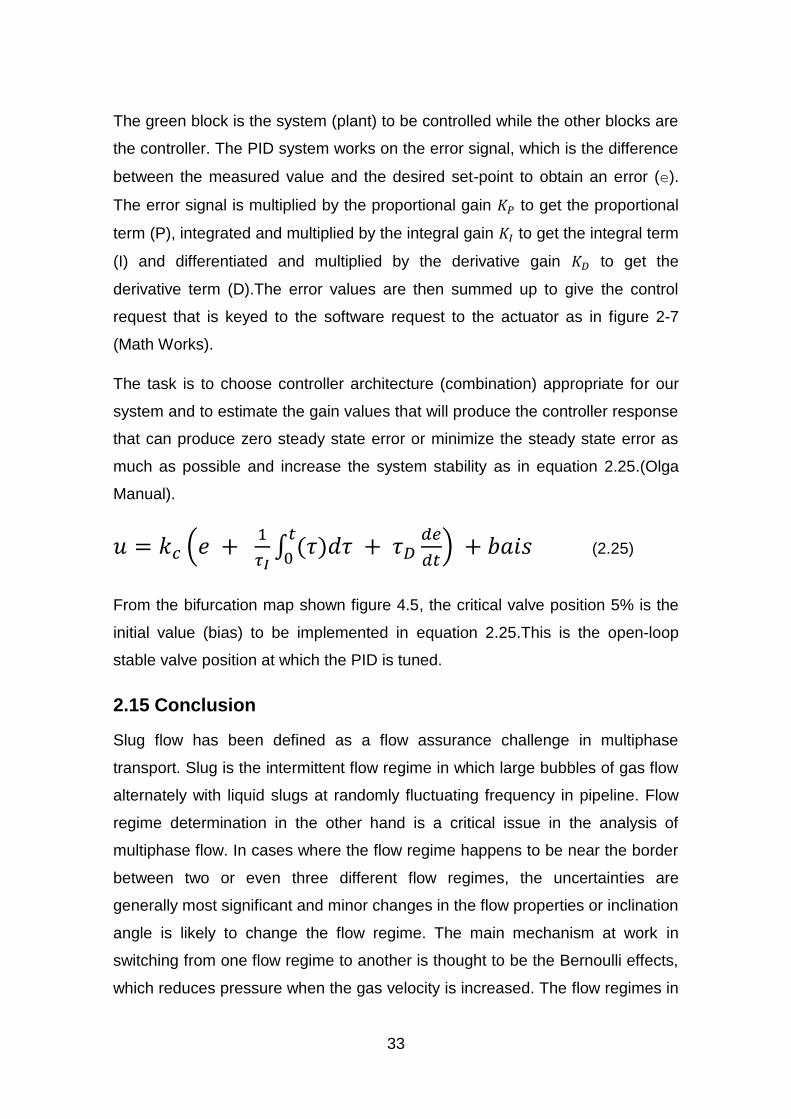
The green block is the system (plant) to be controlled while the other blocks are

the controller. The PID system works on the error signal, which is the difference

between the measured value and the desired set-point to obtain an error (e).

The error signal is multiplied by the proportional gain to get the proportional

term (P), integrated and multiplied by the integral gain to get the integral term

(I) and differentiated and multiplied by the derivative gain to get the

derivative term (D).The error values are then summed up to give the control

request that is keyed to the software request to the actuator as in figure 2-7

(Math Works).

The task is to choose controller architecture (combination) appropriate for our

system and to estimate the gain values that will produce the controller response

that can produce zero steady state error or minimize the steady state error as

much as possible and increase the system stability as in equation 2.25.(Olga

Manual).

(

∫ ( 𝑑

) (2.25)

From the bifurcation map shown figure 4.5, the critical valve position 5% is the

initial value (bias) to be implemented in equation 2.25.This is the open-loop

stable valve position at which the PID is tuned.

2.15 Conclusion

Slug flow has been defined as a flow assurance challenge in multiphase

transport. Slug is the intermittent flow regime in which large bubbles of gas flow

alternately with liquid slugs at randomly fluctuating frequency in pipeline. Flow

regime determination in the other hand is a critical issue in the analysis of

multiphase flow. In cases where the flow regime happens to be near the border

between two or even three different flow regimes, the uncertainties are

generally most significant and minor changes in the flow properties or inclination

angle is likely to change the flow regime. The main mechanism at work in

switching from one flow regime to another is thought to be the Bernoulli effects,

which reduces pressure when the gas velocity is increased. The flow regimes in

34

horizontal pipes differ from the flow regimes in vertical pipes as bubble flow

does not usually exist in small diameter vertical pipes. The traditional model by

Taitel and Dukler are the most applied in flow regime prediction.

The terminologies used in multiphase literatures were also presented in this

chapter. Publication review of slug control techniques were discussed, showing

the evolution of the different techniques that can be used to control slug flow

problems and these include reduction in pipeline diameter, slug catcher,

splitting of the flow into multiple streams, choke valve technology, gas injection

technology, combination of gas injection and topside choke valve, active

feedback control, flow line modification and layout or geometry of the flow line to

avoid a dip and multivariable control. Each method has its own limitation and

capabilities. In other to be able to control the riser base pressure, a control

objective most relevant to oil and gas operation was defined. The controller that

can achieve the systems operational target to stabilise the system at a valve

opening larger than manual choking with zero steady state error or minimized

steady state error was needed.

35

3 MODELLING THE CASE PROBLEM

An industrial scale case study of 6km flow-line and 46.2m high riser originally

developed by Burke and Kashou 1996 was modelled in Olga 7.1.3 by (Hazem,

2012) and adapted for the current work for the investigation of the effectiveness

of feedback control for hydrodynamic slug mitigation with pressure variation

measurement used to analyse the performance of the system using pressure

transmitter PT at the riser base as controlled variable. Whereas (Hazem, 2012)

model investigated the use of gas injection to control hydrodynamic slugging,

the current work applied topside choking with pressure transmitter PT at the

riser base to investigate the effectiveness of active feedback control to mitigate

hydrodynamic slugging.

The research integrates active feedback control for hydrodynamic slug control

using topside choke valve to assure smooth flow and improve oil production and

recovery.

3.1 Building Olga Model for the Numerical Simulation.

Olga model for the numerical simulation was built using the Burke and Kashou

(1996) model as a starting point.

3.2 Introduction.

Numerical simulation is a machine thinking approach in predicting transient

multiphase flow behaviour in pipeline. A number of software is available in the

market to deal with numerical analysis of multiphase problems. OLGA is one of

the most used and tested software in the market. Olga 7.1.3 is used in this

thesis to study the effectiveness of feedback control and choking at the topside

to mitigate hydrodynamic slugging.

A case study of West African platform suffering hydrodynamic slug flow

was described by (Burke and Kashou,1996).The paper was used as

starting point to build an Olga model. The aim was to obtain result similar

to that of (Burke and Kashou 1996), observing how well matched is the

holdup at the bottom of the riser as a validation of the model.

36

Manual choking of the valve opening was investigated till stability was

attained. The maximum percentage valve opening to attain stability was

recorded. Stabilisation is attained when the holdup and pressure

oscillation at the riser top and riser base are reduced or eliminated.

A Hopf bifurcation map of the manual choke was generated from simulation and

a PI controller was designed at the critical valve position.

3.3 Simulation Start Point.

A real case problem was extensively described by Burke and Kashou of an

offshore platform suffering hydrodynamic slug located at West Africa. This case

problem was used as starting point to model the Olga case. The detail of the

case is explained hereunder.

3.4 Pipeline Inlet Flow Rate:

Oil production 5,318 stb/d.

Gas production 5.351MMscf/d.

Water production 257stb/d.

Liquid production 5,575stb/d (oil plus water = 5,318 257).

Gas Oil Ratio (GOR) 1,006scf/stbo.

Gas Liquid Ratio (GLR) 960 scf/stbl.

Water-cut 4.61%.

Oil gravity 31.9 API.

Liquid production, GOR, percentage water-cut and oil gravity is used in the Olga

model, while the rest parameters are obtained from these parameters and PVT

table.

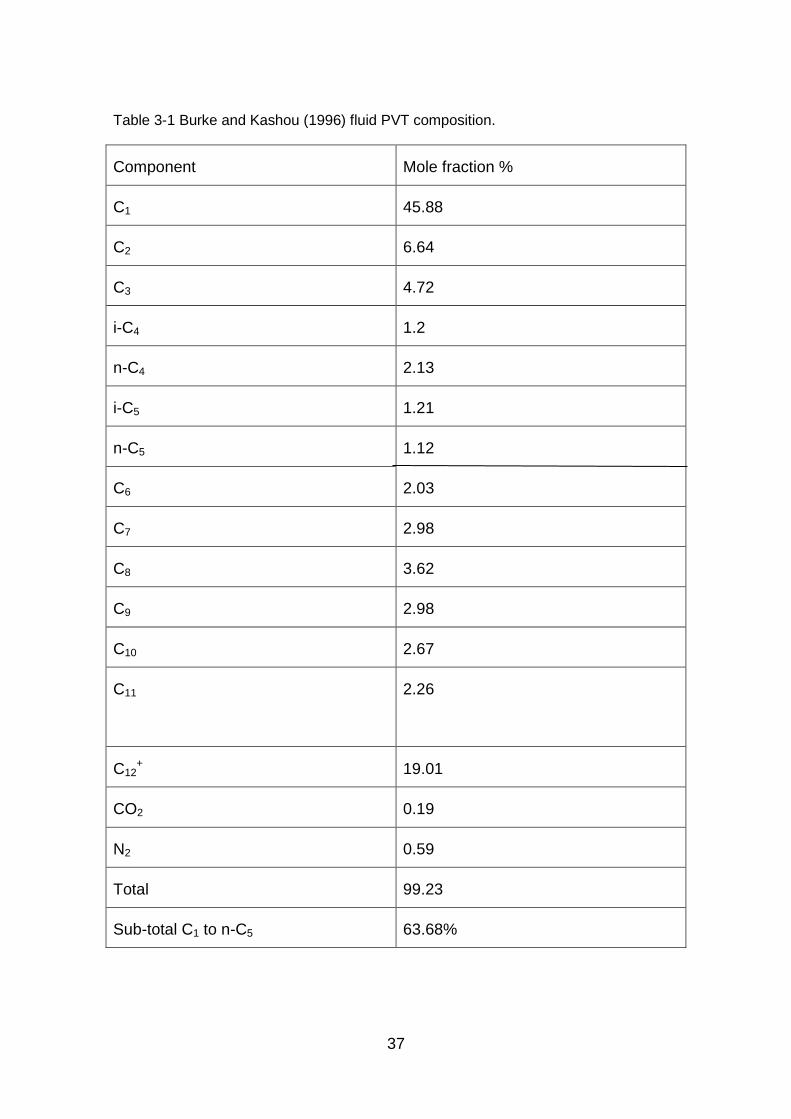
Table 3-1 shows the fluid composition as applied in the fluid PVT calculations.

37

Table 3-1 Burke and Kashou (1996) fluid PVT composition.

Component Mole fraction %

C1 45.88

C2 6.64

C3 4.72

i-C4 1.2

n-C4 2.13

i-C5 1.21

n-C5 1.12

C6 2.03

C7 2.98

C8 3.62

C9 2.98

C10 2.67

C11

2.26

C12+ 19.01

CO2 0.19

N2 0.59

Total 99.23

Sub-total C1 to n-C5 63.68%

38

Gas mole fraction in the fluid composition is the sum of mole fraction of C1 till n-C5 in

Table 3-1 63.68%.

CO2 mole fraction in gas 0.19/63.68x100=0.3%.

N2 mole fraction in gas =0.59/63.68x100=0.93%.

3.5 Pipeline Inlet Condition.

The pipeline inlet condition stated below adapted for the investigation was

initialised in the Olga model window for the numerical simulation.

Pressure in the range 20.3-21.0 bar.

Temperature 83.3 C.

3.6 Pipeline Outlet Condition.

In a similar vein the outlet condition contained below adapted for the

investigation was initialised in the Olga window to specify the outlet condition for

the numerical simulation.

Pressure in the range 11.3-14.8 bar.

Temperature 23.9 C.

3.7 Burke and Kashou (1996) Pipeline Profile.

Detail of (Burke and Kashou, 1996) case study platform profile inlet condition is

explained in figure 3-1 as adapted for the analysis. The case problem definition,

inlet and outlet condition parameters are calculated and initialised in the Olga

window.

.

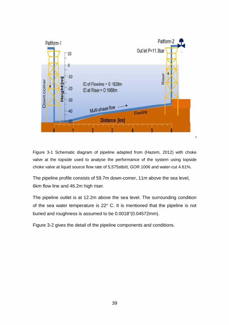
39

Figure 3-1 Schematic diagram of pipeline adapted from (Hazem, 2012) with choke

valve at the topside used to analyse the performance of the system using topside

choke valve at liquid source flow rate of 5,575stb/d, GOR 1006 and water-cut 4.61%.

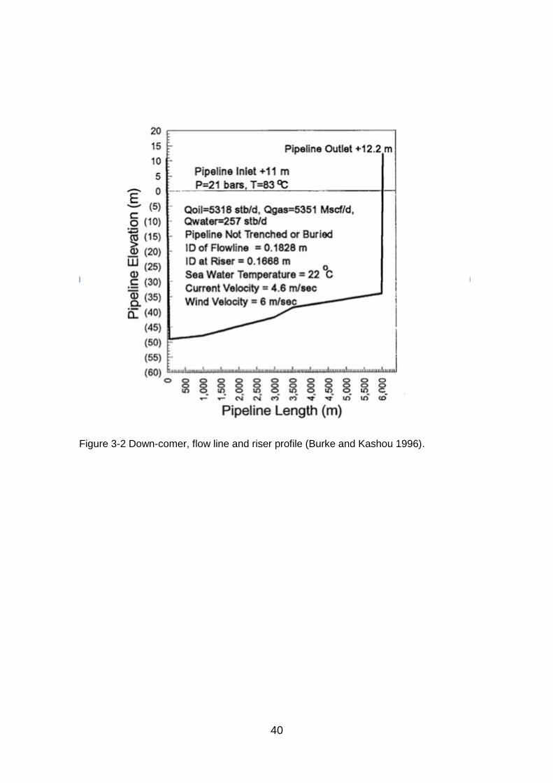
The pipeline profile consists of 59.7m down-comer, 11m above the sea level,

6km flow line and 46.2m high riser.

The pipeline outlet is at 12.2m above the sea level. The surrounding condition

of the sea water temperature is 22 C. It is mentioned that the pipeline is not

buried and roughness is assumed to be 0.0018"(0.04572mm).

Figure 3-2 gives the detail of the pipeline components and conditions.

40

Figure 3-2 Down-comer, flow line and riser profile (Burke and Kashou 1996).

41

Table 3-2 gives more detail of the pipeline component ID, sections, length and

elevations.

Table 3-2 Burke and Kashou (1996) Pipeline Details.

Pipe Description Pipe ID (m) Number of sections Pipeline Length(m) Pipe Elevation(m)

Down comer 0.1668 2 2x29.85 -59.7

Flowline-1 0.1828 10 50,90,8x100 1.2

Flowline-2 0.1828 20 20x100 6.0

Flowline-3 0.1828 5 5x500 3.2

Flowline-4 0.1828 26 24x100,2x50 4.6

Riser 0.1668 2 2x23,1 46.2

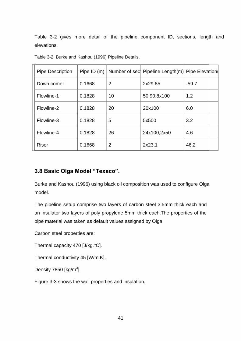
3.8 Basic Olga Model “Texaco”.

Burke and Kashou (1996) using black oil composition was used to configure Olga

model.

The pipeline setup comprise two layers of carbon steel 3.5mm thick each and

an insulator two layers of poly propylene 5mm thick each.The properties of the

pipe material was taken as default values assigned by Olga.

Carbon steel properties are:

Thermal capacity 470 [J/kg. C].

Thermal conductivity 45 [W/m.K].

Density 7850 [kg/m3].

Figure 3-3 shows the wall properties and insulation.

42

Figure 3-3 Properties of carbon steel and poly propylene.

Poly propylene properties are:

Thermal capacity 2000 [J/kg. ].

Thermal conductivity 0.17[W/m.K].

Density 750 [kg/m3].

43

Pipeline was named Wall-1 with the properties shown in figure 3-4.

Figure 3-4 Pipeline wall properties.

An inlet source named oil at the first section of the pipeline was configured as

closed node, implying that analysis was from the wellhead only while the

pipeline outlet was configured as pressure node with pressure set at 11.3bar

and temperature set at 23.9 Figure 3-5 shows the pipeline configuration with

the nodes and the source inlet.

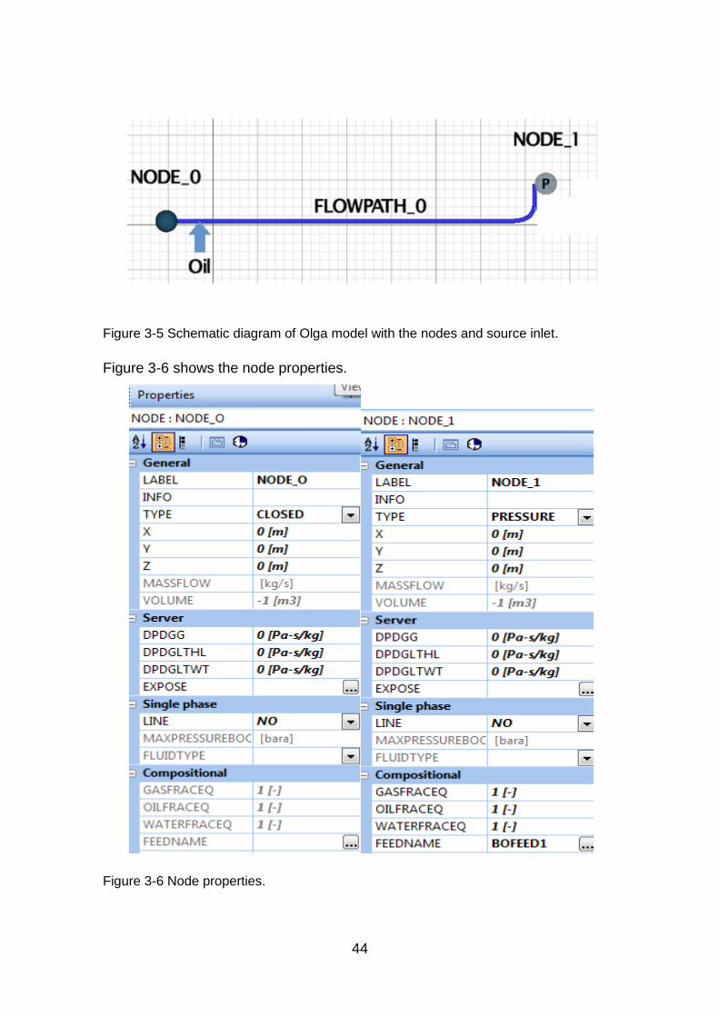
44

Figure 3-5 Schematic diagram of Olga model with the nodes and source inlet.

Figure 3-6 shows the node properties.

Figure 3-6 Node properties.

45

3.9 Geometry of the Pipeline.

The geometry of the pipeline is shown in figure 3-7 with the components.

Figure 3-7 Geometry of the pipeline model Burke and Kashou 1996.

Table 3-3 Detail of pipeline geometry.

Pipe X[m] Y[m] Length[m] Elevation[m] #Sections Length of of

sections(list[m])

Diameter[m] Roughness[m] Wall

Start Point 0 11

Pipe-1 10 11 10 0 4 4:2,5 0.1668 4.5672e-005 Wall-1

Pipe-2 10 -48.7 59.7 -59.7 12 12:4,975 0.1668 4.5672e-005 Wall-1

Pipe-3 949.999 -47.5 940 1.2 20 20:47 0.1828 4.5672e-005 Wall-1

Pipe-4 2949.99 -41.5 2000 6 20 20:100 0.1828 4.5672e-005 Wall-1

Pipe-5 5449.99 -38.3 2500 3.2 20 20:125 0.1828 4.5672e-005 Wall-1

Pipe-6 7949.99 -33.7 2500 4.6 40 40:62,5001 0.1828 4.5672e-005 Wall-1

Pipe-7 7949.99 12.5 46.2 46.2 24 24:1,925 0.1668 4.5672e-005 Wall-1

Pipe-8 7959.99 12.5 10 0 4 4:2,5 0.1668 4.5672e-005 Wall-1

From table 3.3 the pipe diameter in the flow line, riser and down-comer are 0.1828m,

0.1668m and 0.1668m respectively.

3.10 Fluid Composition.

Black oil compositions of three components (gas component, oil component and

water component) were created as contained in the PVT fluid file. Black oil

46

composition was adopted when a detailed fluid property is not available from

the laboratory. The following components were specified from the fluid property:

gas component: specific gravity 1.732, CO2 mole fraction 0.3%, H2S mole

fraction 0% and N2 mole fraction 0.93%

Figure 3-8 Properties of black oil components.

Oil component API 31.9 gravity and water component with specific gravity 1

were initialised in the model. Black oil option was initialised STANDING so that

the correlation used to calculate gas/oil ratio shall be taken as default from Olga

model. Black oil feed (BOFEED-1) the well production feed which consists of

47

three components Oil/Gas/Water with a water- cut of 4.61% and gas oil ratio

GOR of 1006scf/stb were created. The feed properties are shown figure 3-9.

Figure 3-9 Properties of the black oil feed.

3.11 Feed Source

Feed source are assigned to the pipeline with oil installed at the first section of

pipe-1.The well feed BOFEED-1 was assigned to this source with liquid

production of 5,575stb/d at a temperature of 83.3 Gas fraction, oil fraction

and water fraction were kept as default value to take value from the fluid

composition fraction figure 3.10.

Figure 3.10 shows the source properties.

48

Figure 3-10 Source properties.

49

3.12 Options and Integration.

Hydrodynamic slug tracking (HYDSLUG=ON) was turned on, while temperature

calculation on heat transfer from inside pipe wall to the outside was applied.

The rest of Olga values were kept as default, SLUGVOID=SINTEF. This

correlation influenced transition from stratified flow to slug flow significantly

unless slug tracking option is selected (Olga 7.1.3) figure 3.11.

Figure 3-11 OLGA model options and integration.

50

3.13 Slug Tracking.

Hydrodynamic slug tracking initiated DELAYCONSTANT=150 by default as the

number of pipeline diameter a slug will propagate before the next slug is

initiated figure 3.12.

Figure 3-12 Properties of slug tracking options.

51

3.14 Output Options.

The output options were specified in the Olga window for the trend and profile

plots.

3.14.1 Trend and Profile Properties.

The time interval between trend variable printout DTPLOT=10[s] figure 3.13.

Figure 3-13 Trend and profile properties.

3.15 Conclusion

An Olga model was built on the case study. The case definition statement, the

inlet and outlet conditions, the fluid PVT file and the flow geometry were

applied to calculate the parameters that were initialised in the Olga window to

model the dynamic of the case problem in line with the field characteristics.

53

4 SLUG CONTROL DESIGN/TUNING.

4.1 Case Study

The industrial scale case study of 6km flow-line and 46.2m high riser was

modelled in Olga 7.1.3 with pressure variation measurement used to analyse

the performance of the system. The model was validated by comparing the

holdup from the field case oscillation result with the holdup as calculated by

Olga model to ascertain whether a tolerable matching trend result was achieved

as shown in figure 4-1 for the field measurement and olga calculation

respectively.

Figure 4-1 HOL field measurement with HOL as calculated by Olga model.at source

liquid flow rate 5,575 STB/D, 1006scf/d GOR and 4.61% water-cut.

The results were found to match comparatively within an oscillation between 0.2

and 1.0 for the field measurement and between 0.1 and 0.8 for the Olga

54

calculation (both are in the range of 0.8) oscillation trend result and the model

can be assumed valid and favourably matched. However, the field HOL

measurement was 10% under predicted by the Olga calculation. The model is

further validated by a profile plot of the flow regimes as calculated by Olga

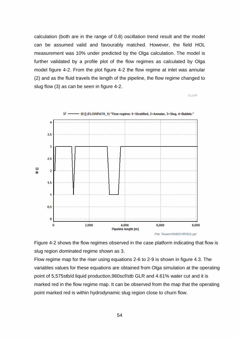
model figure 4-2. From the plot figure 4-2 the flow regime at inlet was annular

(2) and as the fluid travels the length of the pipeline, the flow regime changed to

slug flow (3) as can be seen in figure 4-2.

Figure 4-2 shows the flow regimes observed in the case platform indicating that flow is

slug region dominated regime shown as 3.

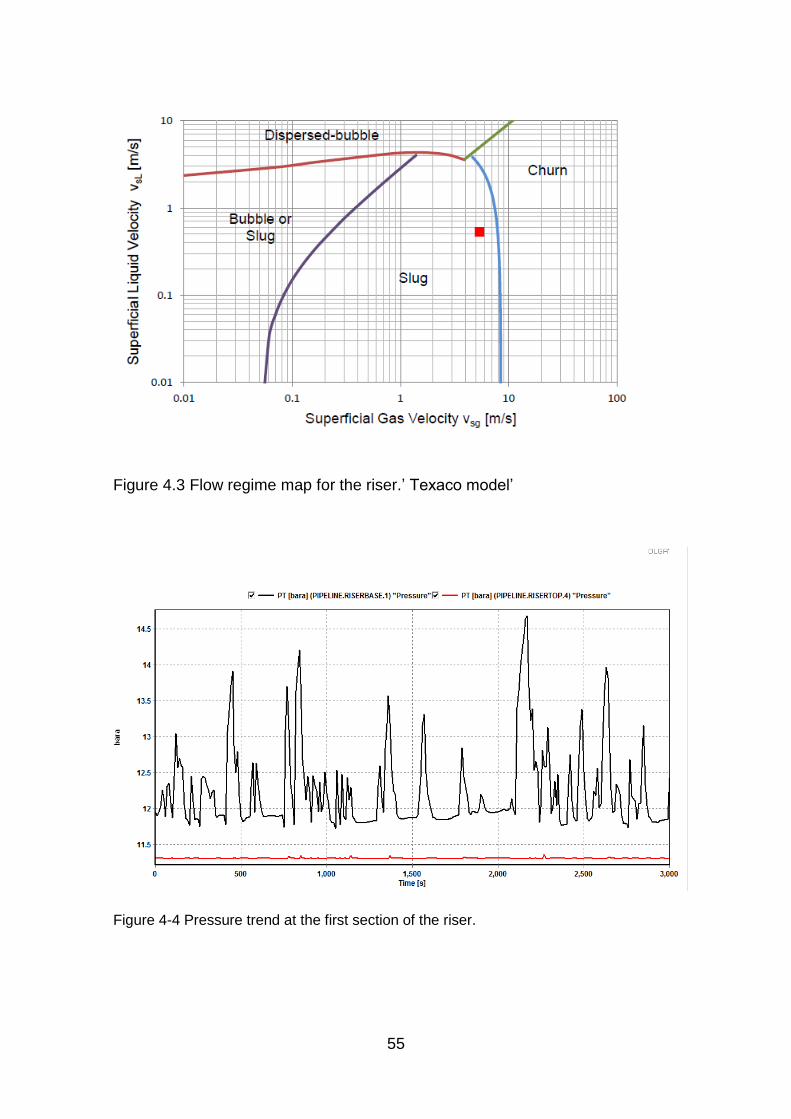
Flow regime map for the riser using equations 2-6 to 2-9 is shown in figure 4.3. The

variables values for these equations are obtained from Olga simulation at the operating

point of 5,575stb/d liquid production,960scf/stb GLR and 4.61% water cut and it is

marked red in the flow regime map. It can be observed from the map that the operating

point marked red is within hydrodynamic slug region close to churn flow.

55

Figure 4.3 Flow regime map for the riser.’ Texaco model’

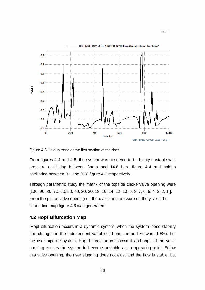
Figure 4-4 Pressure trend at the first section of the riser.

56

Figure 4-5 Holdup trend at the first section of the riser.

From figures 4-4 and 4-5, the system was observed to be highly unstable with

pressure oscillating between 3bara and 14.8 bara figure 4-4 and holdup

oscillating between 0.1 and 0.98 figure 4-5 respectively.

Through parametric study the matrix of the topside choke valve opening were

[100, 90, 80, 70, 60, 50, 40, 30, 20, 18, 16, 14, 12, 10, 9, 8, 7, 6, 5, 4, 3, 2, 1 ].

From the plot of valve opening on the x-axis and pressure on the y- axis the

bifurcation map figure 4.6 was generated.

4.2 Hopf Bifurcation Map

Hopf bifurcation occurs in a dynamic system, when the system loose stability

due changes in the independent variable (Thompson and Stewart, 1986). For

the riser pipeline system, Hopf bifurcation can occur if a change of the valve

opening causes the system to become unstable at an operating point. Below

this valve opening, the riser slugging does not exist and the flow is stable, but

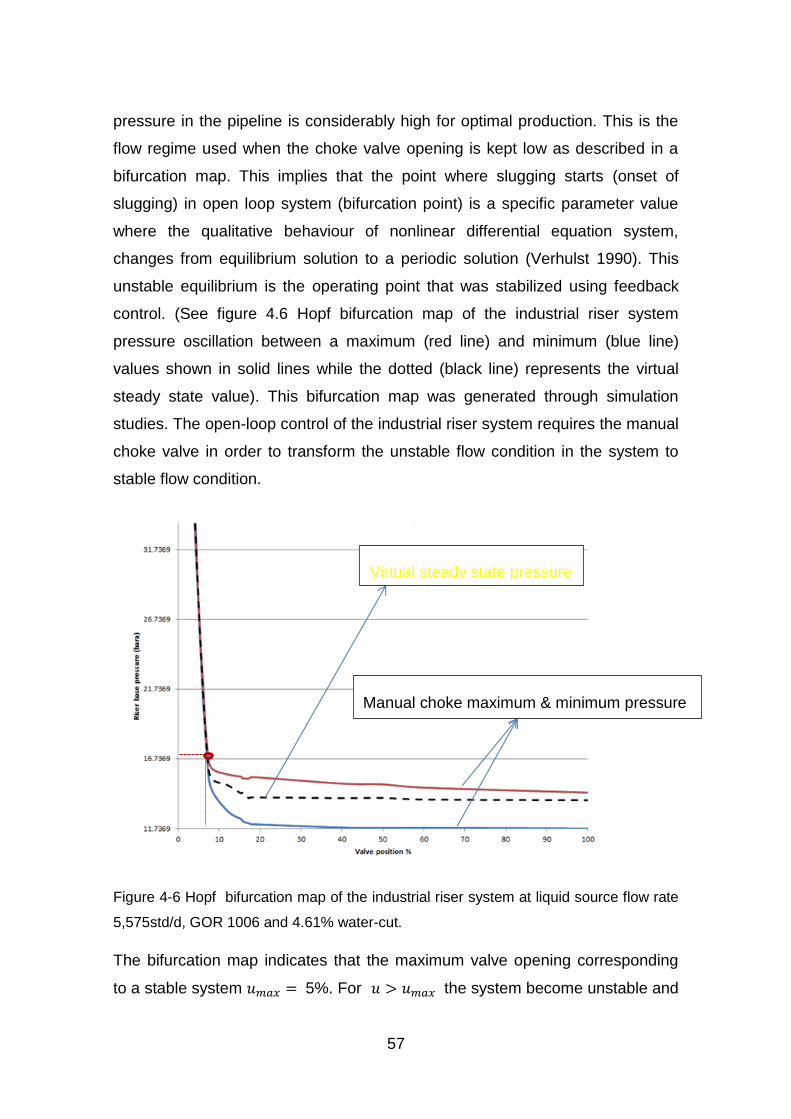
57

pressure in the pipeline is considerably high for optimal production. This is the

flow regime used when the choke valve opening is kept low as described in a

bifurcation map. This implies that the point where slugging starts (onset of

slugging) in open loop system (bifurcation point) is a specific parameter value

where the qualitative behaviour of nonlinear differential equation system,

changes from equilibrium solution to a periodic solution (Verhulst 1990). This

unstable equilibrium is the operating point that was stabilized using feedback

control. (See figure 4.6 Hopf bifurcation map of the industrial riser system

pressure oscillation between a maximum (red line) and minimum (blue line)

values shown in solid lines while the dotted (black line) represents the virtual

steady state value). This bifurcation map was generated through simulation

studies. The open-loop control of the industrial riser system requires the manual

choke valve in order to transform the unstable flow condition in the system to

stable flow condition.

Figure 4-6 Hopf bifurcation map of the industrial riser system at liquid source flow rate

5,575std/d, GOR 1006 and 4.61% water-cut.

The bifurcation map indicates that the maximum valve opening corresponding

to a stable system 5%. For the system become unstable and

Manual choke maximum & minimum pressure

Virtual steady state pressure

58

oscillates between a maximum and minimum pressure values. Thus is

known as the bifurcation point marked red in figure 4-6. The riser base

pressure was calculated from the system for 5% 100%. The critical

value indicated by the bifurcation map gives a minimum pressure 15.3881 bara

and maximum of the system to be stabilized by manual choking. The

interest is to stabilise the system at unstable operating points, where the values

of are larger than this critical value such that the total pressure drop across

the riser and the valve is reduced and thus the overall production is increased.

The Hopf bifurcation map shows the maximum valve opening that can stabilise

the system (open -loop), a maximum manual valve opening of 5% was

achieved. This valve opening is also known as the critical valve opening beyond

which the system will be unstable as in figure 4.6.

At and below this valve position, slugging does not exist and the system can be

operated open-loop stable without oscillation and without control. Above 5%

valve opening, the system becomes unstable, with a pressure oscillation

between a minimum and maximum pressure value as shown by the solid lines

in figure 4.6.while the dotted line represent the virtual steady state pressure

value.

4.3 Controller Design and Tuning

The controller was designed based on the critical values of the bifurcation map

and subsequently tuned when the gain values have been determined.

4.3.1 Methods for Quantifying the Process Gain

The controller that has the capacity to stabilise the system at the predicted

close-loop operating point to achieve the predicted optimal production is

required. The Proportional, Integral and Derivative controller parameters were

calculated with the control objective of a stabilised operation as well as

optimized production. The method for quantifying the process gain is outlined

thus:

59

4.3.1.1 Finding the Process Gain for Open-Loop Stable System.

The process gain values were determined from open-loop system using the

process reaction curve.

4.3.1.1.1 Open Loop Tuning Rules (Process Reaction Curve).

The process reaction curve is an approximation model of the process, assuming

the process behaves as a first order plus time delay system. The process

reaction curve is identified by doing an open loop step test of the system and

then identifying the process model parameters. The following steps were

applied:

Put the controller in manual mode

Allow the process value (Y) to stabilise and not oscillating

Step the output of the PI controller

Collect data and plot the process reaction curve

Repeat making the step in opposite direction

K = process gain; K =

K =

(4.1)

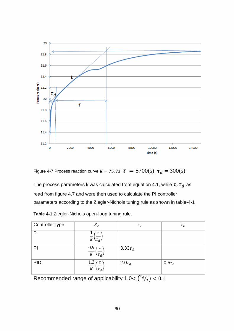
60

Figure 4-7 Process reaction curve 5700(s), 300(s)

The process parameters k was calculated from equation 4.1, while as

read from figure 4.7 and were then used to calculate the PI controller

parameters according to the Ziegler-Nichols tuning rule as shown in table-4-1

Table 4-1 Ziegler-Nichols open-loop tuning rule.

Controller type

P

(

)

PI

(

)

3.33

PID

(

)

2.0 0.5

Recommended range of applicability 1.0 ( 𝑑

⁄ )

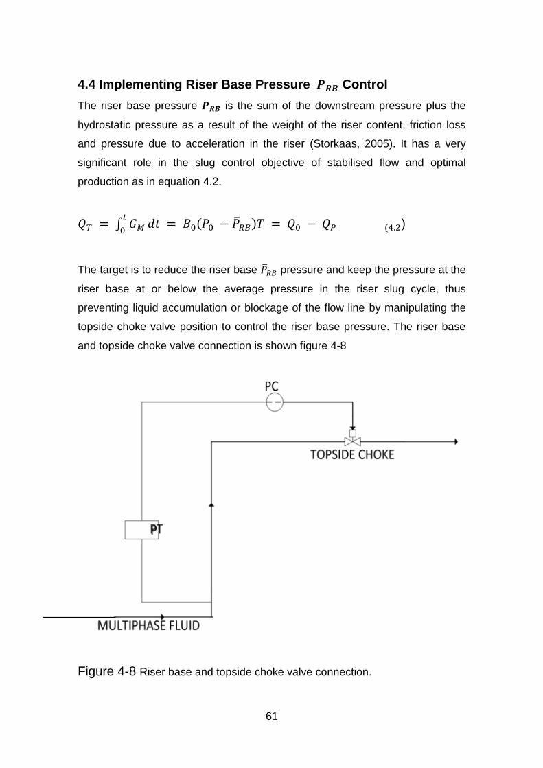
61

4.4 Implementing Riser Base Pressure Control

The riser base pressure is the sum of the downstream pressure plus the

hydrostatic pressure as a result of the weight of the riser content, friction loss

and pressure due to acceleration in the riser (Storkaas, 2005). It has a very

significant role in the slug control objective of stabilised flow and optimal

production as in equation 4.2.

∫

𝑑 ( ( )

The target is to reduce the riser base pressure and keep the pressure at the

riser base at or below the average pressure in the riser slug cycle, thus

preventing liquid accumulation or blockage of the flow line by manipulating the

topside choke valve position to control the riser base pressure. The riser base

and topside choke valve connection is shown figure 4-8

Figure 4-8 Riser base and topside choke valve connection.

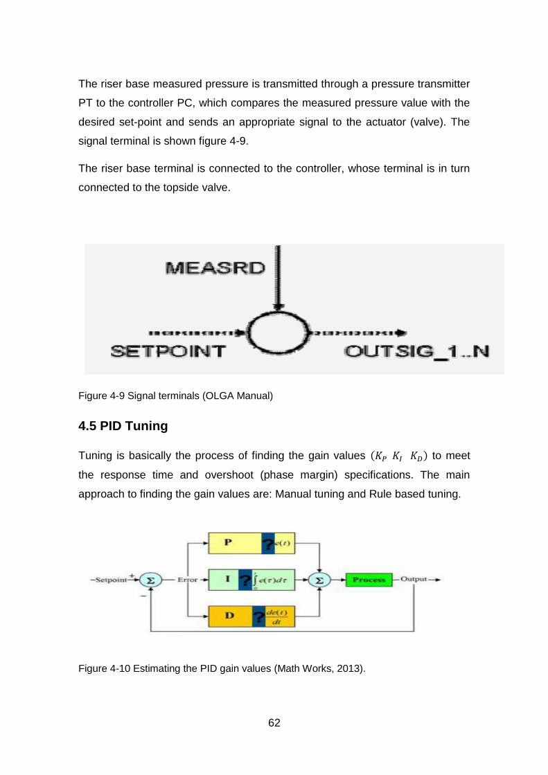
62

The riser base measured pressure is transmitted through a pressure transmitter

PT to the controller PC, which compares the measured pressure value with the

desired set-point and sends an appropriate signal to the actuator (valve). The

signal terminal is shown figure 4-9.

The riser base terminal is connected to the controller, whose terminal is in turn

connected to the topside valve.

Figure 4-9 Signal terminals (OLGA Manual)

4.5 PID Tuning

Tuning is basically the process of finding the gain values ( to meet

the response time and overshoot (phase margin) specifications. The main

approach to finding the gain values are: Manual tuning and Rule based tuning.

Figure 4-10 Estimating the PID gain values (Math Works, 2013).

63

Manual tuning is purely based on trial and error process, time

consuming, non-systematic and requires experience. It may not

produce optimal design and may leads to dangerous conditions for the

plant.

Table 4.2 shows the PI control parameters

Table 4-2 PI tuning parameters.

4.5.1 Open-Loop Tuning

The bifurcation valve position is set as the initial value at which the PI is tuned.

The equivalent value of the controlled variable riser base pressure at the

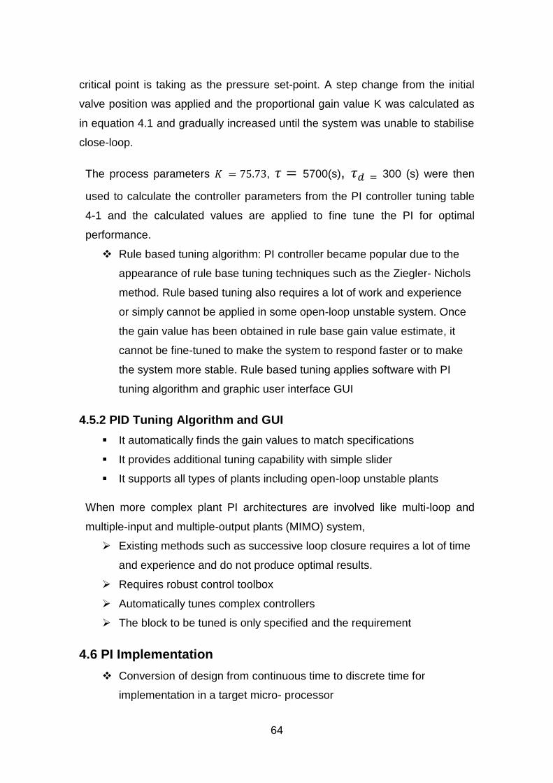
64

critical point is taking as the pressure set-point. A step change from the initial

valve position was applied and the proportional gain value K was calculated as

in equation 4.1 and gradually increased until the system was unable to stabilise

close-loop.

The process parameters , 5700(s), 300 (s) were then

used to calculate the controller parameters from the PI controller tuning table

4-1 and the calculated values are applied to fine tune the PI for optimal

performance.

Rule based tuning algorithm: PI controller became popular due to the

appearance of rule base tuning techniques such as the Ziegler- Nichols

method. Rule based tuning also requires a lot of work and experience

or simply cannot be applied in some open-loop unstable system. Once

the gain value has been obtained in rule base gain value estimate, it

cannot be fine-tuned to make the system to respond faster or to make

the system more stable. Rule based tuning applies software with PI

tuning algorithm and graphic user interface GUI

4.5.2 PID Tuning Algorithm and GUI

It automatically finds the gain values to match specifications

It provides additional tuning capability with simple slider

It supports all types of plants including open-loop unstable plants

When more complex plant PI architectures are involved like multi-loop and

multiple-input and multiple-output plants (MIMO) system,

Existing methods such as successive loop closure requires a lot of time

and experience and do not produce optimal results.

Requires robust control toolbox

Automatically tunes complex controllers

The block to be tuned is only specified and the requirement

4.6 PI Implementation

Conversion of design from continuous time to discrete time for

implementation in a target micro- processor

65

Scaling for fixed-point implementation. If the fixed-point data type is not

scaled, the design that works well in floating point could be completely

wrong on fixed-point implementation.

Generates efficient C-code for the target micro-processor

4.7 Verify if the Design Works

o Testing before hardware prototypes are available.

o Testing corner cases

o Non-linear desktop simulation

1. Testing different operating conditions.

2 Testing different stages of design elaboration.

o Software-in-the loop testing

-Use generated S-function as a way to run the generated controller

code against plant model in Simulink.

4.8 Results:

The reference trajectory (controller) is the red line with time-delay necessary to

approximate the model to first order system figure 4.11 plotted against the

close-loop system response in black line. The gain values are adjusted until the

steady state error was minimized to increase the system stability.

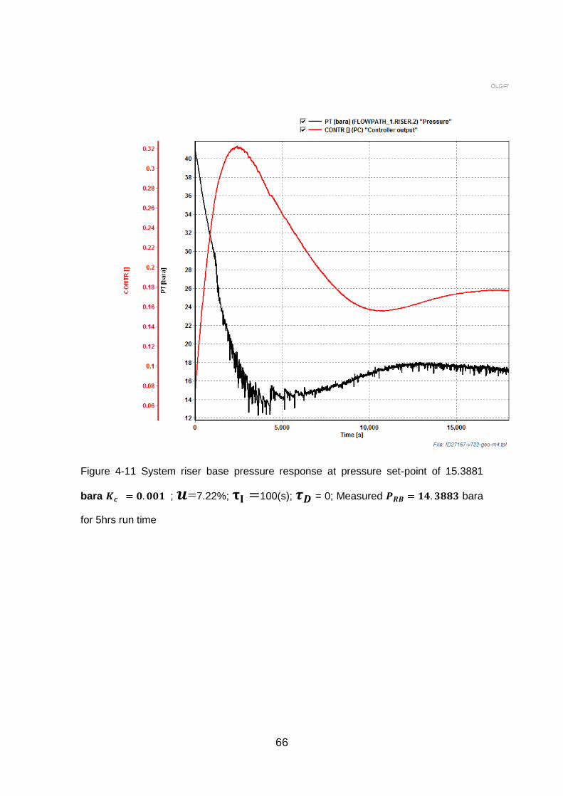
66

Figure 4-11 System riser base pressure response at pressure set-point of 15.3881

bara ; =7.22%; 100(s); = 0; Measured bara

for 5hrs run time

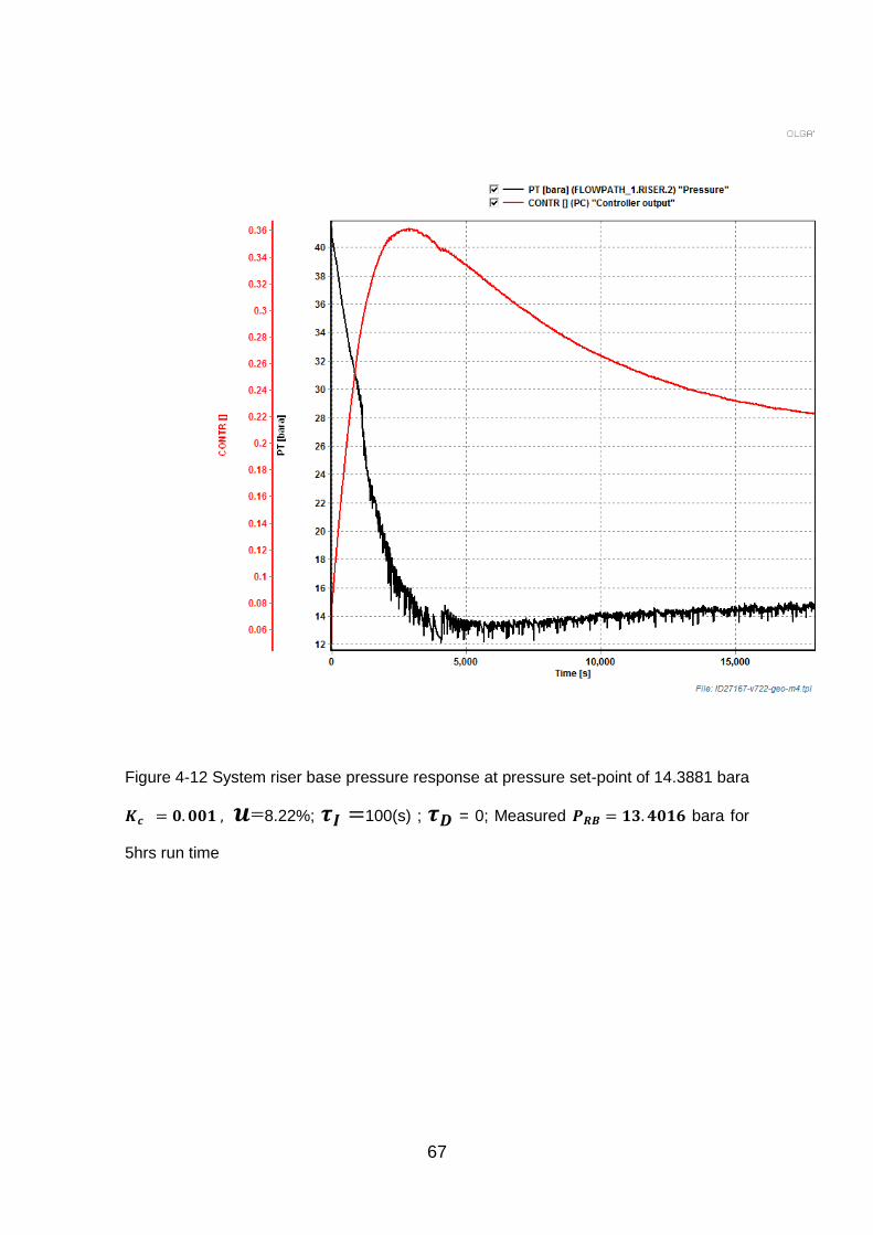
67

Figure 4-12 System riser base pressure response at pressure set-point of 14.3881 bara

=8.22%; 100(s) ; = 0; Measured bara for

5hrs run time

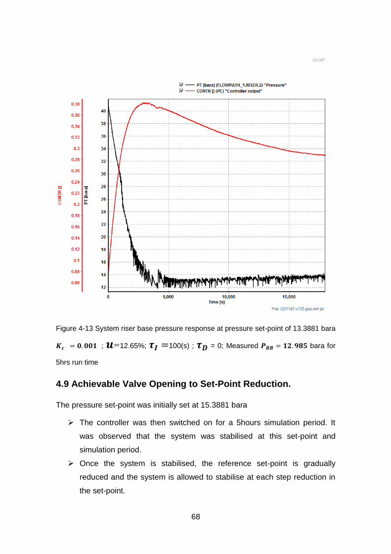
68

Figure 4-13 System riser base pressure response at pressure set-point of 13.3881 bara

; =12.65%; 100(s) ; = 0; Measured bara for

5hrs run time

4.9 Achievable Valve Opening to Set-Point Reduction.

The pressure set-point was initially set at 15.3881 bara

The controller was then switched on for a 5hours simulation period. It

was observed that the system was stabilised at this set-point and

simulation period.

Once the system is stabilised, the reference set-point is gradually

reduced and the system is allowed to stabilise at each step reduction in

the set-point.

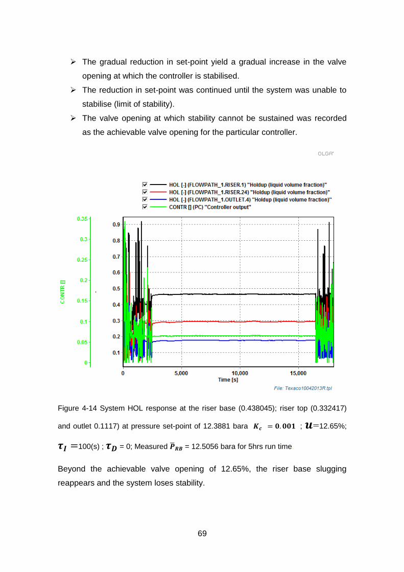
69

The gradual reduction in set-point yield a gradual increase in the valve

opening at which the controller is stabilised.

The reduction in set-point was continued until the system was unable to

stabilise (limit of stability).

The valve opening at which stability cannot be sustained was recorded

as the achievable valve opening for the particular controller.

Figure 4-14 System HOL response at the riser base (0.438045); riser top (0.332417)

and outlet 0.1117) at pressure set-point of 12.3881 bara ; =12.65%;

100(s) ; = 0; Measured = 12.5056 bara for 5hrs run time.

Beyond the achievable valve opening of 12.65%, the riser base slugging

reappears and the system loses stability.

70

4.10 Loss of Stability and Continuous Oscillation.

When the stability limit of the system is exceeded the system oscillates

continuously.

As the proportional gain value is increased the system stability

is lost. The reduction in steady state error happens at the expense

of the system stability, and the integral term was introduced to

eliminate the steady state error, while the derivative term helps to

increase the system stability.

The task of estimating the gain values from the system

hardware is usually base on experience by trial and error and may

not give an optimal gain values.

Integrator windup is another challenge in tuning the PID controller.

Integrator windup happens when the actuator winds fully open or

fully closed and cannot get the desired set-point.

Another issue is due to large integral value that needs to unwind

which takes long time to unwind and this make the system

unstable.

Approximating derivative term (differentiating the error)

introduces noise into the system, since system noise at high

frequency is amplified when it is differentiated.

Another issue encountered in PID usage is to be able to switch

to the different forms P, PI and PID in ideal or parallel form,

output saturation, and integrator anti-windup and bump-less

transfer from one loop to the other in a multi-loop system.

4.11 Effect of Automatic Control of Topside Choke Valve

Opening

The application of automatic PI feedback control on the topside choke valve,

transformed the system to close-loop system and the system operate in the

open-loop unstable region with increased valve opening and reduced riser base

pressure represented by the green and yellow curves (figure 4-16). The

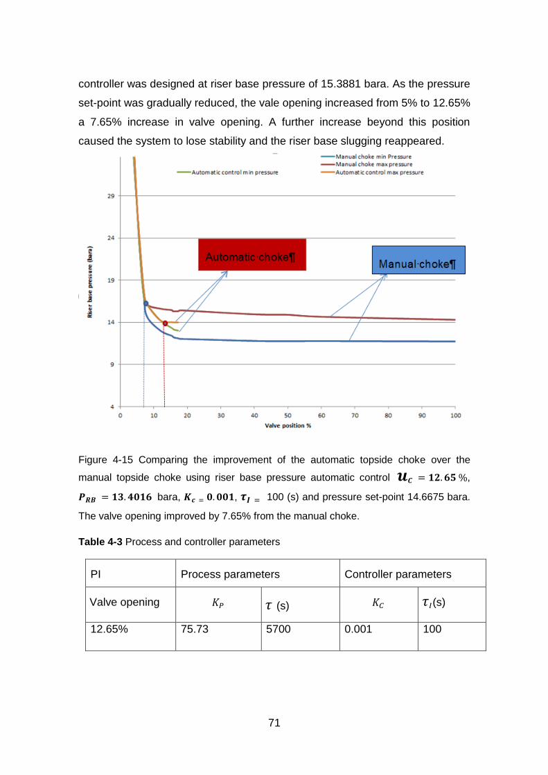
71

controller was designed at riser base pressure of 15.3881 bara. As the pressure

set-point was gradually reduced, the vale opening increased from 5% to 12.65%

a 7.65% increase in valve opening. A further increase beyond this position

caused the system to lose stability and the riser base slugging reappeared.

Figure 4-15 Comparing the improvement of the automatic topside choke over the

manual topside choke using riser base pressure automatic control ,

bara, , 100 (s) and pressure set-point 14.6675 bara.

The valve opening improved by 7.65% from the manual choke.

Table 4-3 Process and controller parameters

PI Process parameters Controller parameters

Valve opening (s) (s)

12.65% 75.73 5700 0.001 100

72

The blue and red solid curves represents the manual choke minimum and

maximum pressures while the green and yellow curves represents the

automatic controller minimum and maximum pressures as compared with the

result of the manual control.

73

5 CONCLUSION / FUTURE WORK

5.1 Conclusion

A review of hydrodynamic slug control techniques, including their applications,

limitations and challenges were discussed in the work. These techniques

include manual choke valve technique, slug catcher, gas-injection, combination

of gas-injection and choking, active feedback control of the topside choke, flow

line modification/layout to avoid dips and splitting of flow into multiple streams.

From the result of the investigation obtained from Olga simulation it was found

thus:

The use of manual topside choke valve alone as control strategy results in

low valve opening 5%.

The application of automatic feedback control on the topside choke valve

resulted in operating the system in the open-loop unstable region.

The application of feedback control improved the choke valve opening from

5% to 12.65%, a confirmation of Ogazi’s finding that operating control at

open-loop condition improves the valve opening more than manual choke.

From the improvement on the valve opening to larger valve, feedback

control is capable of improving the performance of the system at a reduced

riser base pressure.

Feedback control was able to stabilise the system and at limited valve

opening of 12.65% achievable.

There was significant reduction in back-pressure by implementing control at

open-loop condition from 15.3881bara to 13.4016bara.

Active feedback control showed interesting result in suppressing

hydrodynamic slug with reduced back-pressure than manual choke

The interesting results were the capability to operate the system in the open-

loop unstable region.

Lower back-pressure than using manual choke method thus supressing the

riser base slugging.

74

The valve opening was increased from 5% to 12.65% with active control

representing more than 100% increase in the valve opening, when

compared with manual choke.

This translates to an improvement in production.

FUTURE WORK:

Extensive work is still required in order to gain sufficient knowledge and

understanding of hydrodynamic slugs and its control.

It is recommended that the model be investigated on reservoir source.

The model is recommended for validation with experimental data.

Economic analysis to determine if the control strategy can be

implemented on the reference case suffering hydrodynamic slugging is

recommended.

Another control variable should be investigated to determine which

control variable can yield largest valve opening.

75

REFERENCES

Ansari, M.R, (1998). Dynamical behavior of slug initiation generated by short

waves in two-phase air-water stratified flow. ASME HTD 361. 289-295

Åström, K. J., & Hägglund, T. (1995). Automatic tuning of simple regulators with

specifications on phase and amplitude margins. Automatic a, 20(5), 645-651.

Barnea, D. (1977), A unified model for predicting flow-pattern transitions for the

whole range of pipeline inclinations. International Journal of Multiphase

Flow, vol.13, no. 1

Burke, N. E. and Kashou, S. F. (1996), Slug-sizing/slug-volume prediction:

State of the art review and simulation", SPE Production and Facilities, vol.

11, no. 3, pp. 166-172.

Bratland, O. (2010), Pipe flow 2 Multiphase flow assurance,

drbratland.com,Norway

British Standard (2005), Natural gas. Standard reference conditions, BS EN ISO

13443:2005, British standard, London, UK

Cao, Y., Omotayo, M., Lao, L. and Yeung, H. (2011), A study on active gas lift

control for hydrodynamic slug mitigation, 11/YC/56, Cranfield University,

Bedfordshire, UK.

Crowe,C.T.(2009), Multiphase Flow Handbook.

http://www.ftp2share.com/file/26667/Multiphase%20Flow%20Handbook.rar.

html

Fabre, J. Line, A. Peresson, L. (1992). Two fluid/two flow pattern model for

transient gas liquid flow in pipes. In 4th International conference on

Multiphase Flow, Nice, pp 269-284

Handbook of Multiphase Flow Metering, (MPFM Handbook) (2005), Revision 2,

Norwegian Society for Oil and Gas Measurement (NFOGM), Oslo, Norway

Hazem, K; Yi Cao and Liyun Lao (2012), Gas Injection for hydrodynamic slug

control. Proceedings of the 2012 IFAC Workshop on Automatic Control in

Offshore Oil and Gas Production, Norwegian University of Science and

Technology, Trondheim, Norway,

May 31- June 1, 2012

76

Hill, T.(1990), Gas injection at riser base solves slugging flow problems. Oil and

Gas Journal, (USA),vol.88, no.9

Issa, R.I and Kempf, M.H.W, 2003. Simulation of slug flow in horizontal and

near horizontal pipes with two-fluid model. International Journal of

Multiphase Flow. Pergamon

Jansen, F.E. (1990), Elimination of severe slugging in a pipeline-riser system. A

Master of Science thesis submitted at the Graduate School, University of

Tulsa.

Jansen, F. E. and Shoham, O. (1994), "Methods for eliminating pipeline -risers

flow instabilities", Society of Petroleum Engineers Journal,

Jansen, F. E., Shoham, O. and Taitel, Y. (1996), "The elimination of severe

slugging—experiments and modelling", International Journal of Multiphase

Flow, vol. 22, no. 6, pp. 1055-1072.

Math Works, PID tuning <webinar@em.mathworks.com.

Mehrdad,P.Fard, John-Morten Godhavn and Svein, Ivar Sagatun. (2006)

Modelling of severe slug and slug control with OLGA. SPE International

symposium and exhibition on formation damage control. Lafayette,

Louisiana

OLGA user manual version 7.1.2

Ogazi, A I, Ogunkolade, S, Cao, Y, Lao, L and Yeung, H. (2009) Severe

slugging control through open loop unstable pid tuning to increase oil

production. 14th International Conference on Multiphase Production

Technology, Cannes, France

Ogazi, A.I, Cao, Y, Lao, L and Yeung, H. (2011),Production potential of severe

slugging control system.18th International Federation of Automatic Control

(IFAC) World Congress. August, 28-September,2 2011 Milano Italy.

Ogazi, A. I, Cao, Y, Yeung, H and Lao, L. (2010), Slug control in large valve

openings to maximize oil production, Journal of Society of Petroleum

Engineers. SPE

77

Ogunnaike, B A. and Ray, W H. (1994). Process dynamics, modelling and

control, Oxford University Press, New York.

Oram, P (2013) Control application in industries, delivering breakthrough

solution.www.bp.com

Schmidt, Z., Brill, P. J. and Beggs, D. H. (1980), Experimental study of severe

slugging in a Two-phase-flow pipeline-riser pipe system, vol. 20, no. 5

Schmidt, Z., Doty, D. R. and Dutta-Roy, K. (1985), Severe slugging in offshore

pipeline riser-pipe systems, vol. 25, no. 1.

Seborg, D E, Edgar, T F, Mellichamp, D A, Doyle III, F J (2004), Process

dynamics and control, Wiley

Shoham, O. (2006), Mechanistic Modelling of gas-liquid two-phase flow in

pipes, Society of Petroleum Engineers, New York

Skogestad, S and Postlethwiate, I (2005), Multivariable feedback control. John

Wiley & Sons Ltd

Storkaas, E (2005), Anti-slug control in pipeline riser systems. PHD Thesis,

Norwegian University of Science and Technology

Taitel, Y. (1986), Stability of severe slugging, International Journal of Multiphase

Flow, vol. 12, no. 2, pp. 203--217.

Taitel, Y. and Dukler, A. E. (1976), Model for predicting flow regime transitions

in horizontal and near horizontal gas-liquid low, AIChE Journal, vol. 22, no.

1, pp. 47-55.

Taitel, Y., Barnea, D. and Duckler, A. (1980), Modeling flow pattern transitions

for steady upward gas-liquid flow in vertical tubes, AICHE, , no. 26, pp. 345.

Taitel, Y., Barnea, D, (1990).Two-phase slug flow. Advanced Heat Transfer 20,

83-132

Thompson, J.M.T. and Stewart, H.B. (1986). Nonlinear dynamics and chaos.

John Wiley and Sons Ltd Chichester Great Britain, 1st edition

Yocum, B. T. (1973), Offshore riser slug flow avoidance: Mathematical models

for design and optimization", SPE European Meeting, 01/01/1973, London

Varne Valle, (2010) Field experience and analysis of hydrodynamic slugging.

Dynamic simulation seminar, Oct. 20 2010. www.statoil.com

78

Verhulst, F.A. (1990), Nonlinear differential equations and dynamical systems.

New York: Springer-Verlag

79

Appendix A Matrices of manual and automatic control

A.1 Comparing manual choke and automatic control (maximum

and minimum pressures)

Manual choke Automatic control

Valve

opening

(%)

Minimum

pressure

(bara)

Maximum

pressure(bara)

Minimum

pressure(bara)

Maximum

pressure(bara)

4 33.611 35.3721 33.611 35.3721

5 27.5164 27.8193 27.5164 27.8193

6 21.358 22.4285 21.358 22.4285

7 17.0904 17.8133 17.0904 17.8133

8 14.6532 16.1231 16.1231 16.1231

12 14.6532 16.1231 16.1231 16.1231

15.35 12.4081 15.4532 14.2156 14.2756

15.69 12.3081 15.3201 13.2387 14.0125

16.02 12.2031 15.321 13.1387 14.0035

17.27 12.1081 15.321 13.0287 14.002

18 12.042 15.427

40 11.7999 14.9564

50 11.7682 14.9015

60 11.7815 14.665

100 11.7369 14.3081

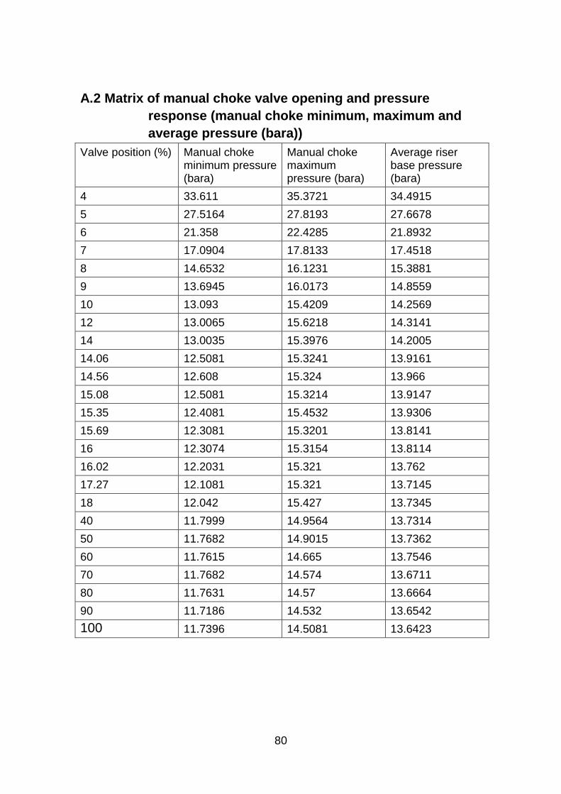
80

A.2 Matrix of manual choke valve opening and pressure

response (manual choke minimum, maximum and

average pressure (bara))

Valve position (%) Manual choke minimum pressure (bara)

Manual choke maximum pressure (bara)

Average riser base pressure (bara)

4 33.611 35.3721 34.4915

5 27.5164 27.8193 27.6678

6 21.358 22.4285 21.8932

7 17.0904 17.8133 17.4518

8 14.6532 16.1231 15.3881

9 13.6945 16.0173 14.8559

10 13.093 15.4209 14.2569

12 13.0065 15.6218 14.3141

14 13.0035 15.3976 14.2005

14.06 12.5081 15.3241 13.9161

14.56 12.608 15.324 13.966

15.08 12.5081 15.3214 13.9147

15.35 12.4081 15.4532 13.9306

15.69 12.3081 15.3201 13.8141

16 12.3074 15.3154 13.8114

16.02 12.2031 15.321 13.762

17.27 12.1081 15.321 13.7145

18 12.042 15.427 13.7345

40 11.7999 14.9564 13.7314

50 11.7682 14.9015 13.7362

60 11.7615 14.665 13.7546

70 11.7682 14.574 13.6711

80 11.7631 14.57 13.6664

90 11.7186 14.532 13.6542

100 11.7396 14.5081 13.6423