Embed Size (px)
Citation preview
Worked examples and exercises are in the textSTROUD
PROGRAMME 28
PROBABILITY
Worked examples and exercises are in the textSTROUD
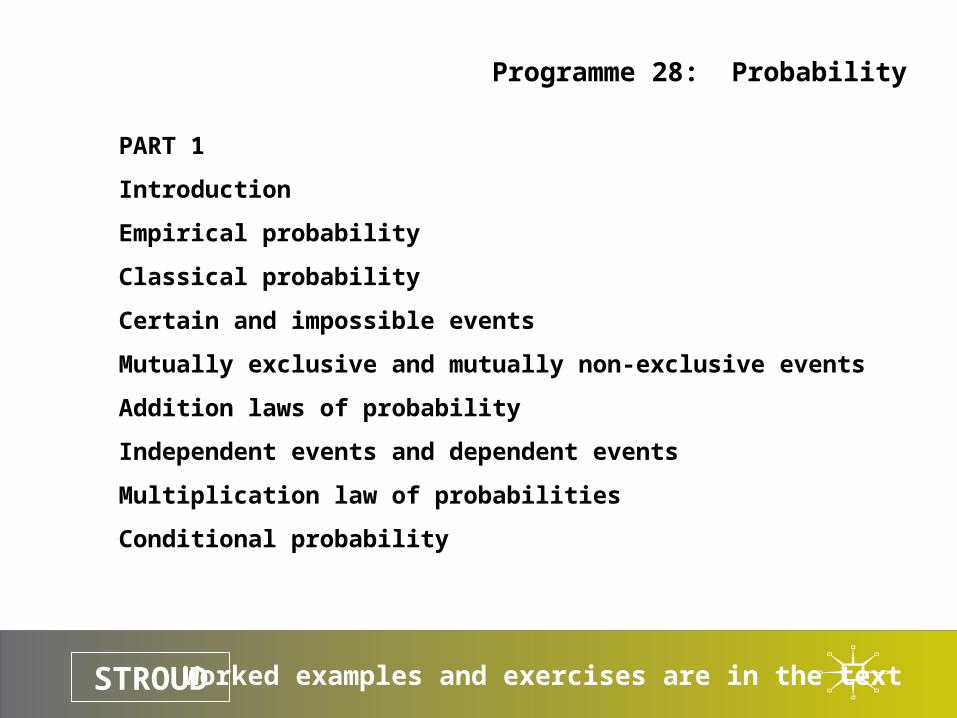
Programme 28: Probability
PART 1
Introduction
Empirical probability
Classical probability
Certain and impossible events
Mutually exclusive and mutually non-exclusive events
Addition laws of probability
Independent events and dependent events
Multiplication law of probabilities
Conditional probability
Worked examples and exercises are in the textSTROUD
Programme 28: Probability
Introduction
Notation
Types of probability
Worked examples and exercises are in the textSTROUD
Programme 28: Probability
Introduction
Notation
Every trial or experiment has one or more possible outcomes. For example, rolling a six-sided die is a trial with six possible outcomes. An event, denoted by A, is a collection of one or more of those outcomes. For example, throwing an even number in the roll of a six-sided die is an event which consists of three outcomes.
The probability, denoted by P(A) of an event A is a measure of the likelihood of the event occurring in any one trial or experiment.
The probabilities of the various events associated with a trial can be defined in one of two ways.
Worked examples and exercises are in the textSTROUD
Programme 28: Probability
Introduction
Types of probability
The probabilities of the various events associated with a trial can be defined either:
(a) Empirically: by repeating the experiment a number of times and noting the relative frequencies of the events.
(b) Classically: by defining the probabilities beforehand based on a knowledge of the experiment and its possible outcomes.
Worked examples and exercises are in the textSTROUD
Programme 28: Probability
PART 1
Introduction
Empirical probability
Classical probability
Certain and impossible events
Mutually exclusive and mutually non-exclusive events
Addition laws of probability
Independent events and dependent events
Multiplication law of probabilities
Conditional probability
Worked examples and exercises are in the textSTROUD
Programme 28: Probability
Empirical probability
Expectation
Success or failure
Multiple samples
Experiment
Worked examples and exercises are in the textSTROUD
Programme 28: Probability
Empirical probability
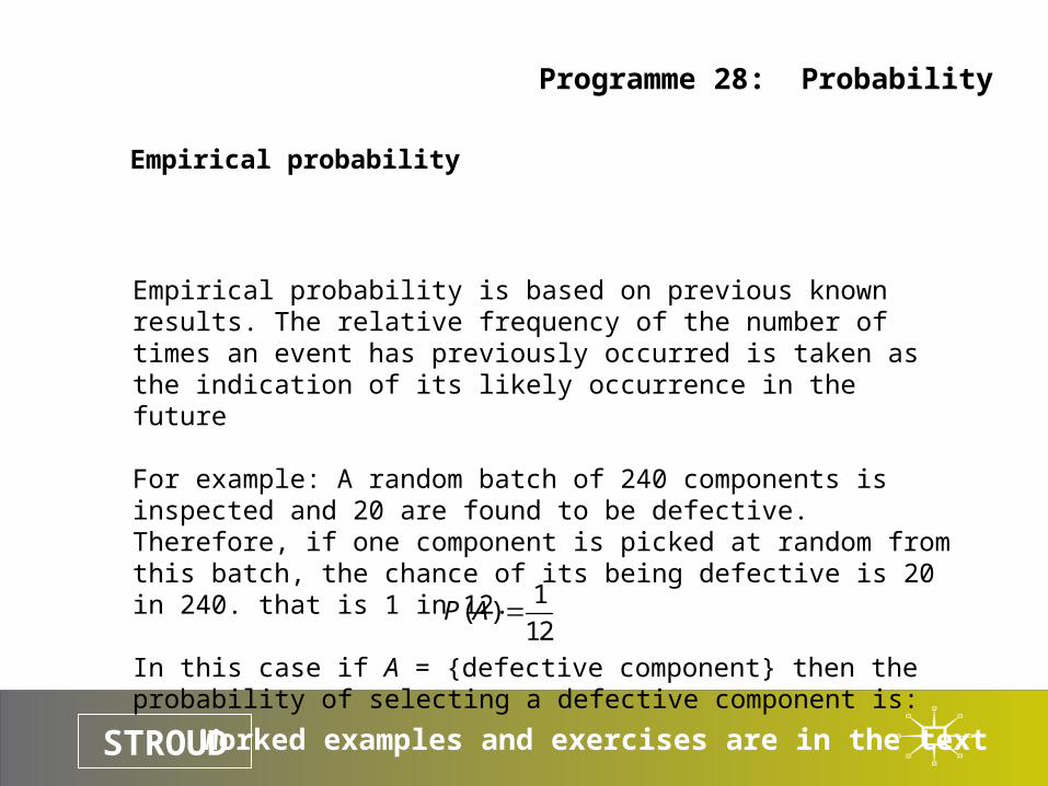
Empirical probability is based on previous known results. The relative frequency of the number of times an event has previously occurred is taken as the indication of its likely occurrence in the future
For example: A random batch of 240 components is inspected and 20 are found to be defective. Therefore, if one component is picked at random from this batch, the chance of its being defective is 20 in 240. that is 1 in 12.
In this case if A = {defective component} then the probability of selecting a defective component is:
1( )
12P A
Worked examples and exercises are in the textSTROUD
Programme 28: Probability
Empirical probability
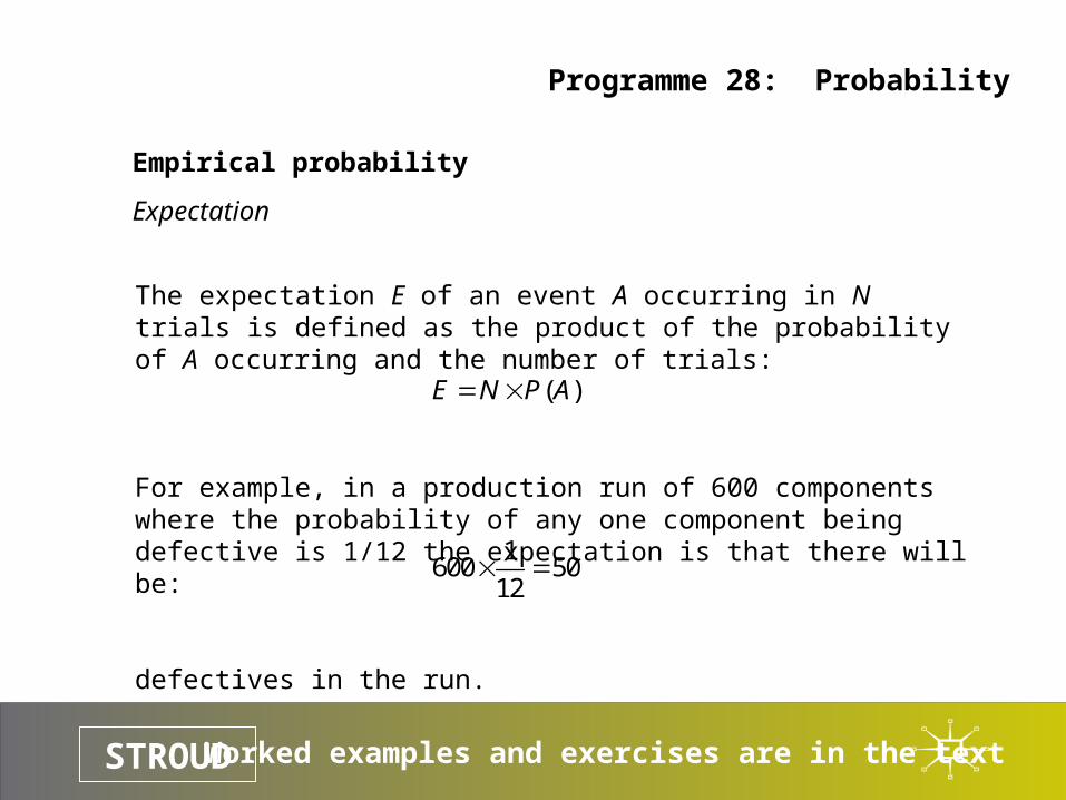
Expectation
The expectation E of an event A occurring in N trials is defined as the product of the probability of A occurring and the number of trials:
For example, in a production run of 600 components where the probability of any one component being defective is 1/12 the expectation is that there will be:
defectives in the run.
( )E N P A
1600 50
12
Worked examples and exercises are in the textSTROUD
Programme 28: Probability
Empirical probability
Success or failure
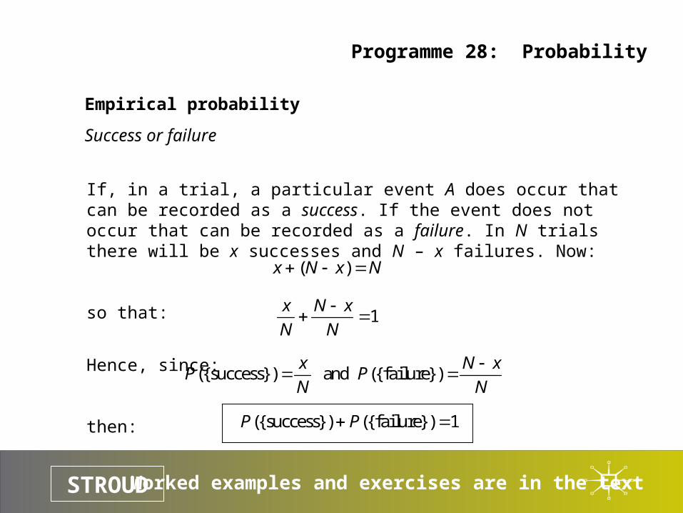
If, in a trial, a particular event A does occur that can be recorded as a success. If the event does not occur that can be recorded as a failure. In N trials there will be x successes and N – x failures. Now:
so that:
Hence, since:
then:
( )x N x N
1x N x
N N
({success}) and ({failure})x N x
P PN N
({success}) ({failure}) 1P P
Worked examples and exercises are in the textSTROUD
Programme 28: Probability
Empirical probability
Success or failure
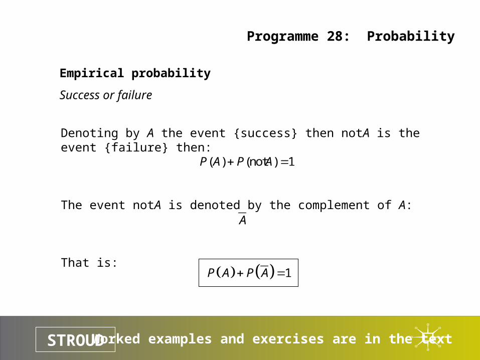
Denoting by A the event {success} then notA is the event {failure} then:
The event notA is denoted by the complement of A:
That is:
( ) (not ) 1P A P A
A
1P A P A
Worked examples and exercises are in the textSTROUD
Programme 28: Probability
Empirical probability
Multiple samples
A single sample of size n taken from a total population of size N is not necessarily representative of the population.
Another sample of size n could well display different properties.
However, continued sampling will provide a cumulative effect that does demonstrate consistency.
Worked examples and exercises are in the textSTROUD
Programme 28: Probability
Empirical probability
Experiment
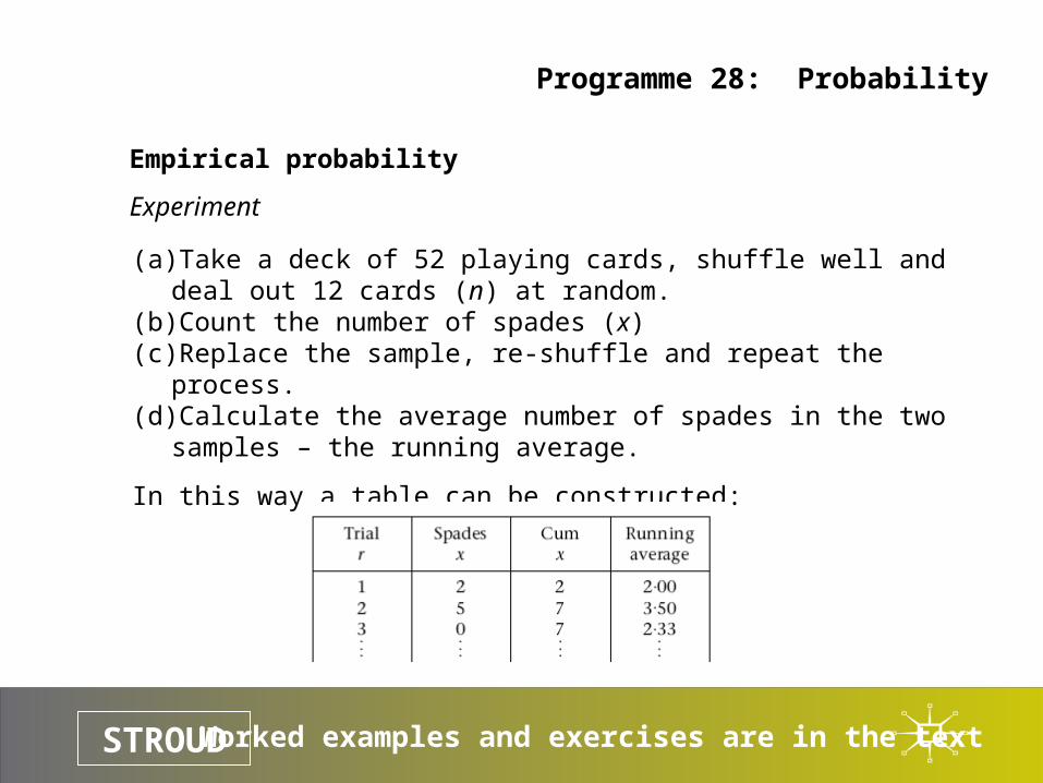
(a) Take a deck of 52 playing cards, shuffle well and deal out 12 cards (n) at random.
(b) Count the number of spades (x)(c) Replace the sample, re-shuffle and repeat the process.(d) Calculate the average number of spades in the two samples – the running
average.
In this way a table can be constructed:
Worked examples and exercises are in the textSTROUD
Programme 28: Probability
Empirical probability
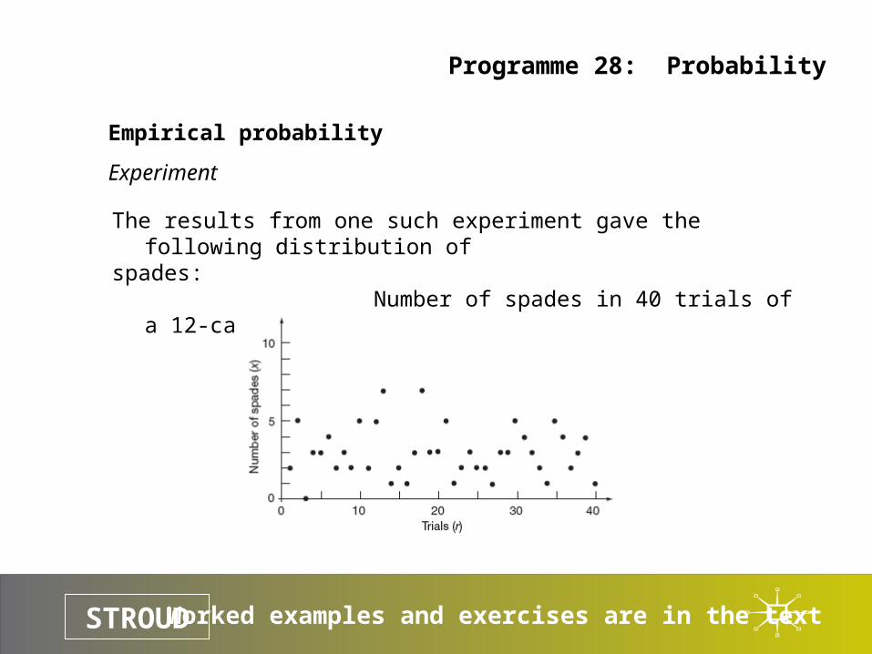
Experiment
The results from one such experiment gave the following distribution of spades: Number of spades in 40 trials of a 12-card sample
Worked examples and exercises are in the textSTROUD
Programme 28: Probability
Empirical probability
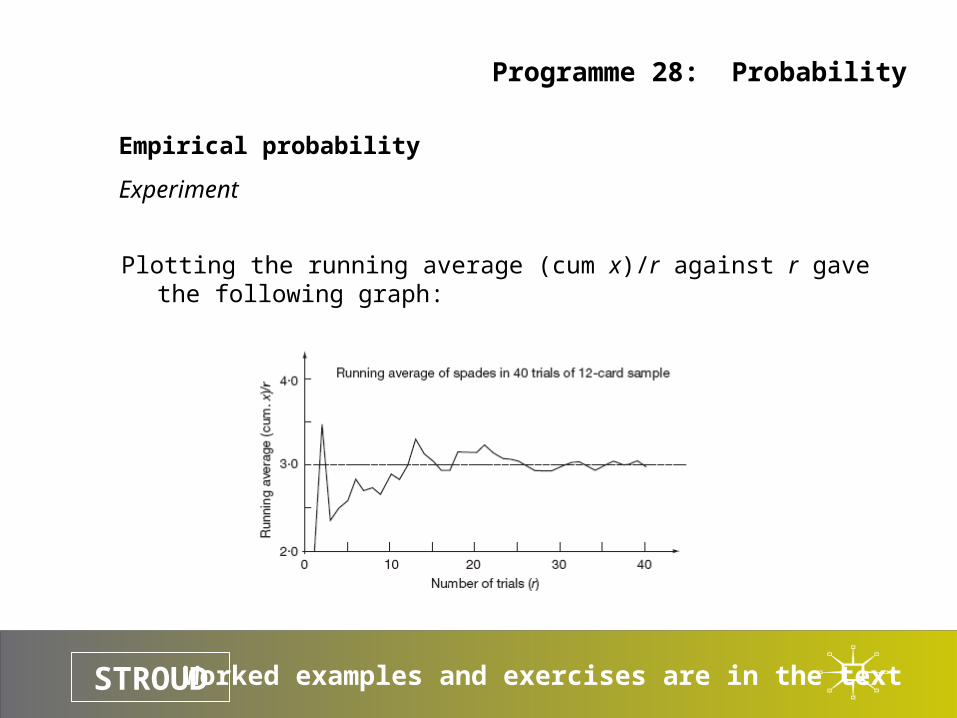
Experiment
Plotting the running average (cum x)/r against r gave the following graph:

Worked examples and exercises are in the textSTROUD
Programme 28: Probability
Empirical probability
Experiment
From the graph it is seen that the running average is settling down to a value of 3 spades in a sample of 12 cards.
Since there are 13 spades in a deck of 52 playing cards there is an expectation that there will be:
Spades in a sample of 12 – but this is taking us towards the second way of defining probabilities.
1312 3
52
Worked examples and exercises are in the textSTROUD
Programme 28: Probability
PART 1
Introduction
Empirical probability
Classical probability
Certain and impossible events
Mutually exclusive and mutually non-exclusive events
Addition laws of probability
Independent events and dependent events
Multiplication law of probabilities
Conditional probability
Worked examples and exercises are in the textSTROUD
Programme 28: Probability
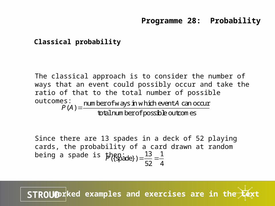
Classical probability
The classical approach is to consider the number of ways that an event could possibly occur and take the ratio of that to the total number of possible outcomes:
Since there are 13 spades in a deck of 52 playing cards, the probability of a card drawn at random being a spade is then:
number of ways in which event can occur( )
total number of possible outcomes
AP A
13 1({spade})
52 4P
Worked examples and exercises are in the textSTROUD
Programme 28: Probability
PART 1
Introduction
Empirical probability
Classical probability
Certain and impossible events
Mutually exclusive and mutually non-exclusive events
Addition laws of probability
Independent events and dependent events
Multiplication law of probabilities
Conditional probability
Worked examples and exercises are in the textSTROUD
Programme 28: Probability
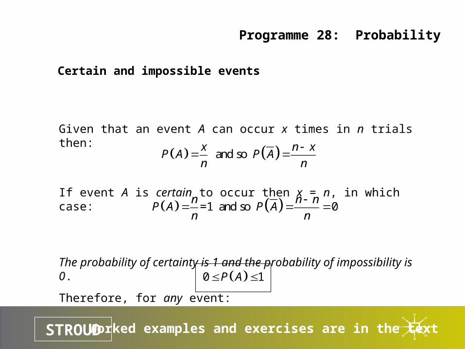
Certain and impossible events
Given that an event A can occur x times in n trials then:
If event A is certain to occur then x = n, in which case:
The probability of certainty is 1 and the probability of impossibility is 0.
Therefore, for any event:
and so x n x
P A P An n
=1 and so 0n n n
P A P An n
0 1P A
Worked examples and exercises are in the textSTROUD
Programme 28: Probability
PART 1
Introduction
Empirical probability
Classical probability
Certain and impossible events
Mutually exclusive and mutually non-exclusive events
Addition laws of probability
Independent events and dependent events
Multiplication law of probabilities
Conditional probability

Worked examples and exercises are in the textSTROUD
Programme 28: Probability
Mutually exclusive and mutually non-exclusive events
Mutually exclusive events are events that cannot occur together. For example, in rolling a six-sided die a 5 and a 6 cannot be rolled at the same time in any one trial.
Mutually non-exclusive events are events that can occur simultaneously. For example, in rolling a six-sided die a 6 and an even number can be rolled at the same time in any one trial
Worked examples and exercises are in the textSTROUD
Programme 28: Probability
PART 1
Introduction
Empirical probability
Classical probability
Certain and impossible events
Mutually exclusive and mutually non-exclusive events
Addition laws of probability
Independent events and dependent events
Multiplication law of probabilities
Conditional probability
Worked examples and exercises are in the textSTROUD
Programme 28: Probability
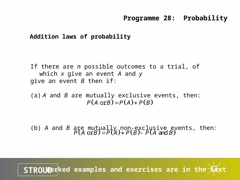
Addition laws of probability
If there are n possible outcomes to a trial, of which x give an event A and y give an event B then if:
(a) A and B are mutually exclusive events, then:
(b) A and B are mutually non-exclusive events, then:
or P A B P A P B
or and P A B P A P B P A B
Worked examples and exercises are in the textSTROUD
Programme 28: Probability
PART 1
Introduction
Empirical probability
Classical probability
Certain and impossible events
Mutually exclusive and mutually non-exclusive events
Addition laws of probability
Independent events and dependent events
Multiplication law of probabilities
Conditional probability
Worked examples and exercises are in the textSTROUD
Programme 28: Probability
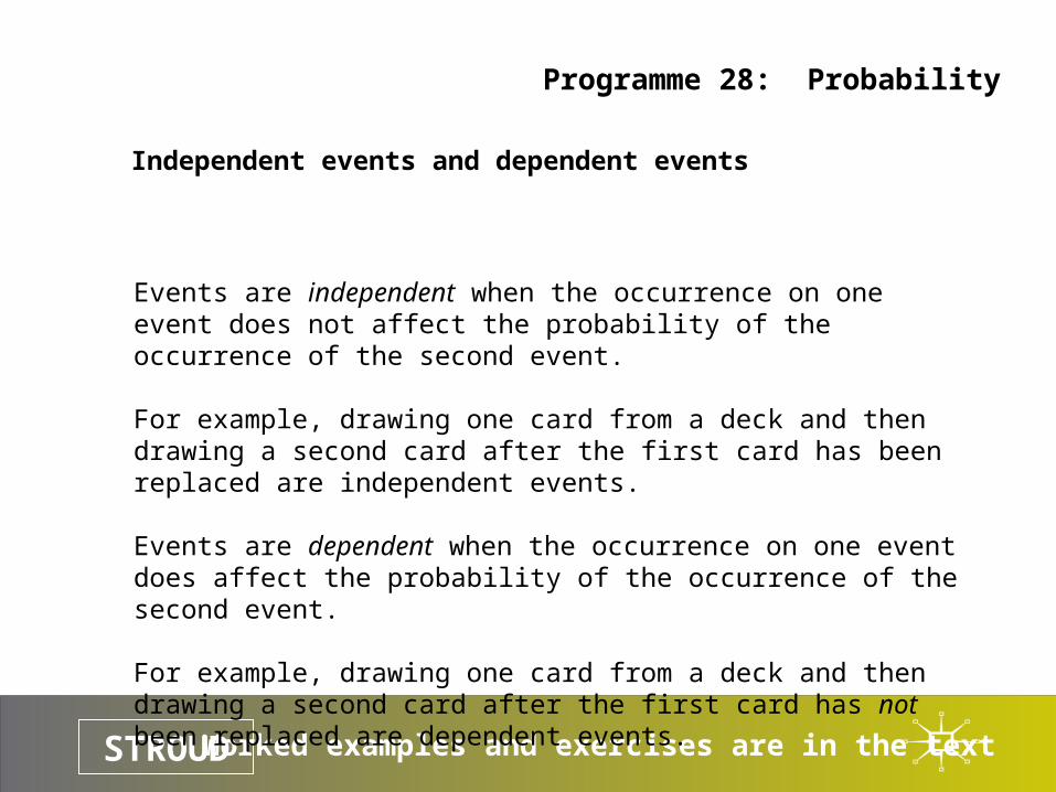
Independent events and dependent events
Events are independent when the occurrence on one event does not affect the probability of the occurrence of the second event.
For example, drawing one card from a deck and then drawing a second card after the first card has been replaced are independent events.
Events are dependent when the occurrence on one event does affect the probability of the occurrence of the second event.
For example, drawing one card from a deck and then drawing a second card after the first card has not been replaced are dependent events.
Worked examples and exercises are in the textSTROUD
Programme 28: Probability
PART 1
Introduction
Empirical probability
Classical probability
Certain and impossible events
Mutually exclusive and mutually non-exclusive events
Addition laws of probability
Independent events and dependent events
Multiplication law of probabilities
Conditional probability
Worked examples and exercises are in the textSTROUD
Programme 28: Probability
Multiplication law of probabilities
If events A and B are independent events then:
and P A B P A P B
Worked examples and exercises are in the textSTROUD
Programme 28: Probability
PART 1
Introduction
Empirical probability
Classical probability
Certain and impossible events
Mutually exclusive and mutually non-exclusive events
Addition laws of probability
Independent events and dependent events
Multiplication law of probabilities
Conditional probability
Worked examples and exercises are in the textSTROUD
Programme 28: Probability
Conditional probability
The probability of event B occurring given that event A has already occurred is denoted by:
If A and B are independent events the prior occurrence of event A will have no effect on the probability of the occurrence of B and so:
If A and B are dependent events the prior occurrence of event A will have an effect on the probability of the occurrence of B and in this case:
P B A
P B A P B
and P A B P A P B A
Worked examples and exercises are in the textSTROUD
Programme 28: Probability
PART 2
Discrete probability distribution
Permutations and combinations
General binomial distribution
Mean and standard deviation of a probability distribution
The Poisson probability distribution
Continuous probability distributions
Standard normal curve
Worked examples and exercises are in the textSTROUD
Programme 28: Probability
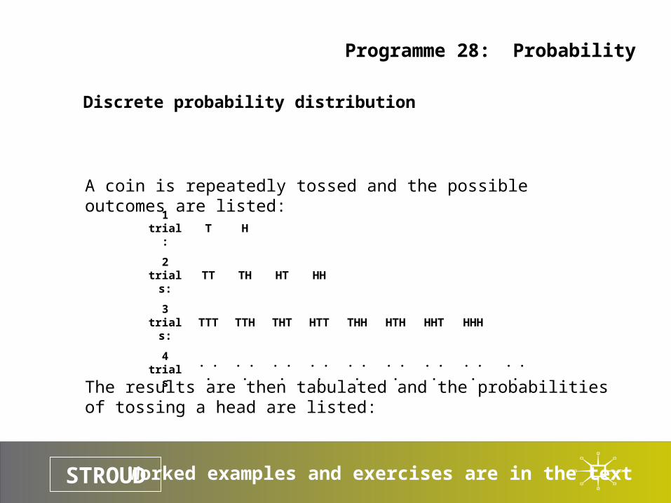
Discrete probability distribution
A coin is repeatedly tossed and the possible outcomes are listed:
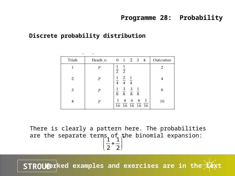
The results are then tabulated and the probabilities of tossing a head are listed:
1 trial: T H
2 trials: TT TH HT HH
3 trials: TTT TTH THT HTT THH HTH HHT HHH
4 trials . . . . . . . . . . . . . . . . . . . . . . . . . . .
Worked examples and exercises are in the textSTROUD
Programme 28: Probability
Discrete probability distribution
There is clearly a pattern here. The probabilities are the separate terms of the binomial expansion:
1 1
2 2
n
Worked examples and exercises are in the textSTROUD
Programme 28: Probability
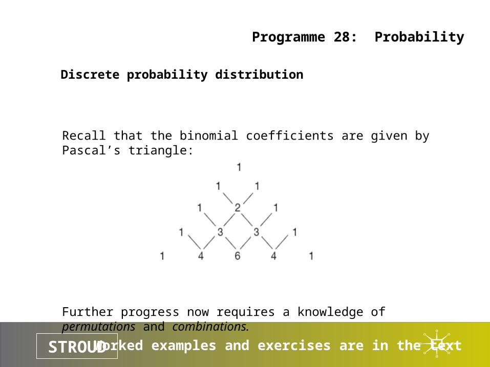
Discrete probability distribution
Recall that the binomial coefficients are given by Pascal’s triangle:
Further progress now requires a knowledge of permutations and combinations.
Worked examples and exercises are in the textSTROUD
Programme 28: Probability
PART 2
Discrete probability distribution
Permutations and combinations
General binomial distribution
Mean and standard deviation of a probability distribution
The Poisson probability distribution
Continuous probability distributions
Standard normal curve
Worked examples and exercises are in the textSTROUD
Programme 28: Probability
Permutations and combinations
Permutations
Combinations
Worked examples and exercises are in the textSTROUD
Programme 28: Probability
Permutations and combinations
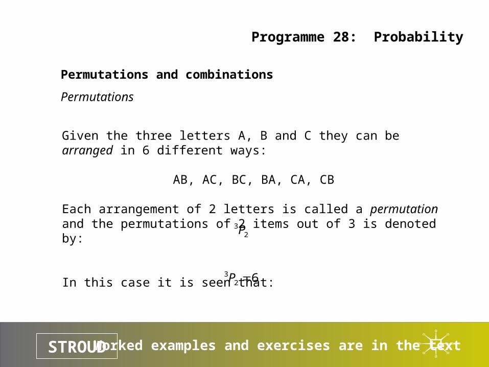
Permutations
Given the three letters A, B and C they can be arranged in 6 different ways:
AB, AC, BC, BA, CA, CB
Each arrangement of 2 letters is called a permutation and the permutations of 2 items out of 3 is denoted by:
In this case it is seen that:
32P
32 6P
Worked examples and exercises are in the textSTROUD
Programme 28: Probability
Permutations and combinations
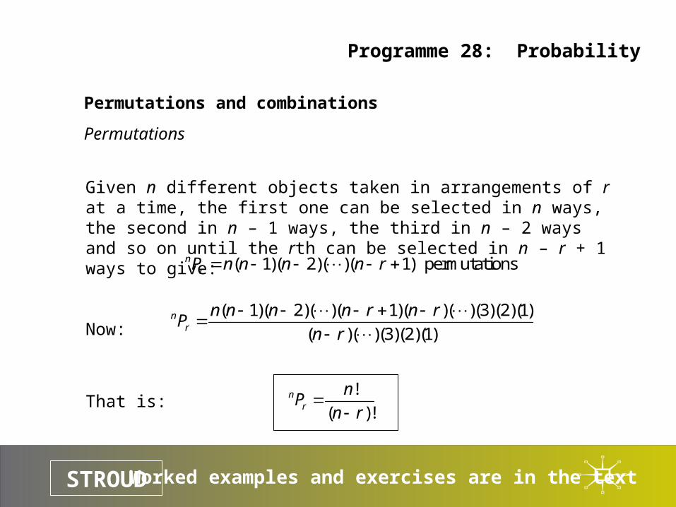
Permutations
Given n different objects taken in arrangements of r at a time, the first one can be selected in n ways, the second in n – 1 ways, the third in n – 2 ways and so on until the rth can be selected in n – r + 1 ways to give:
Now:
That is:
( 1)( 2)( )( 1) permutationsnrP n n n n r
( 1)( 2)( )( 1)( )( )(3)(2)(1)
( )( )(3)(2)(1)n
r
n n n n r n rP
n r
!
( )!n
r
nP
n r
Worked examples and exercises are in the textSTROUD
Programme 28: Probability
Permutations and combinations
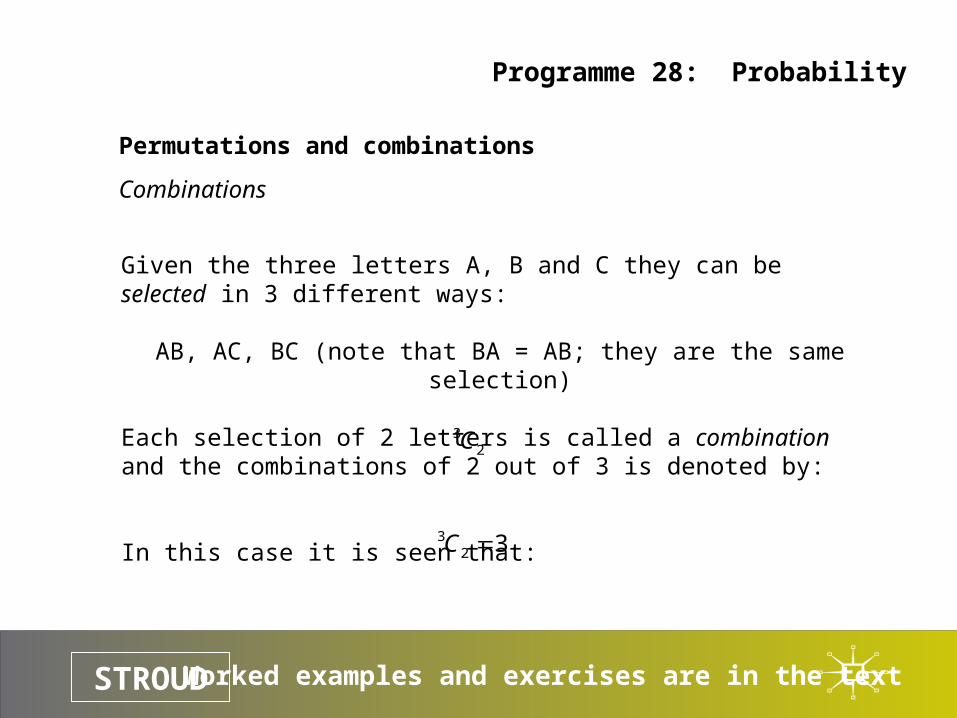
Combinations
Given the three letters A, B and C they can be selected in 3 different ways:
AB, AC, BC (note that BA = AB; they are the same selection)
Each selection of 2 letters is called a combination and the combinations of 2 out of 3 is denoted by:
In this case it is seen that:
32C
32 3C
Worked examples and exercises are in the textSTROUD
Programme 28: Probability
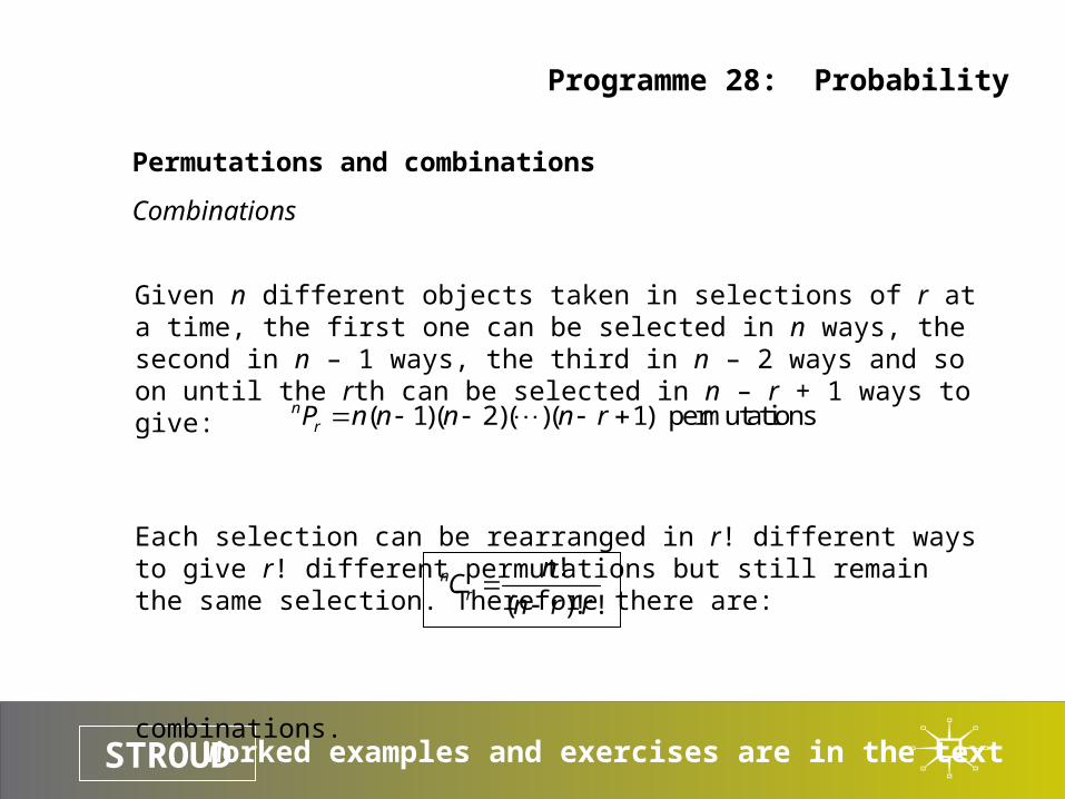
Permutations and combinations
Combinations
Given n different objects taken in selections of r at a time, the first one can be selected in n ways, the second in n – 1 ways, the third in n – 2 ways and so on until the rth can be selected in n – r + 1 ways to give:
Each selection can be rearranged in r! different ways to give r! different permutations but still remain the same selection. Therefore there are:
combinations.
( 1)( 2)( )( 1) permutationsnrP n n n n r
!
( )! !n
r
nC
n r r
Worked examples and exercises are in the textSTROUD
Programme 28: Probability
PART 2
Discrete probability distribution
Permutations and combinations
General binomial distribution
Mean and standard deviation of a probability distribution
The Poisson probability distribution
Continuous probability distributions
Standard normal curve
Worked examples and exercises are in the textSTROUD
Programme 28: Probability
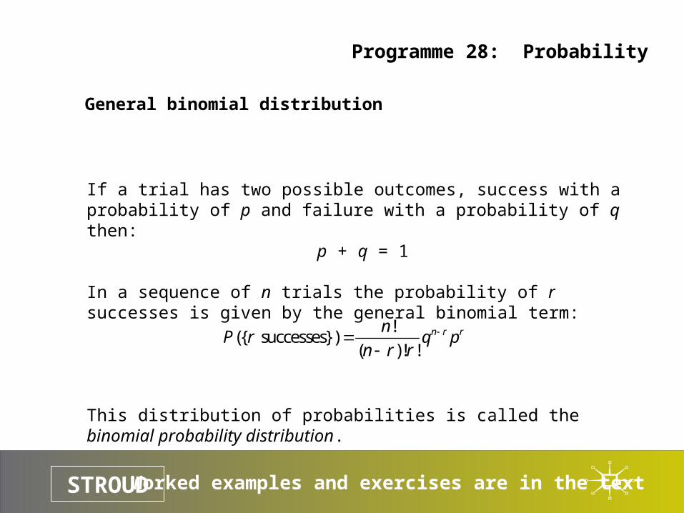
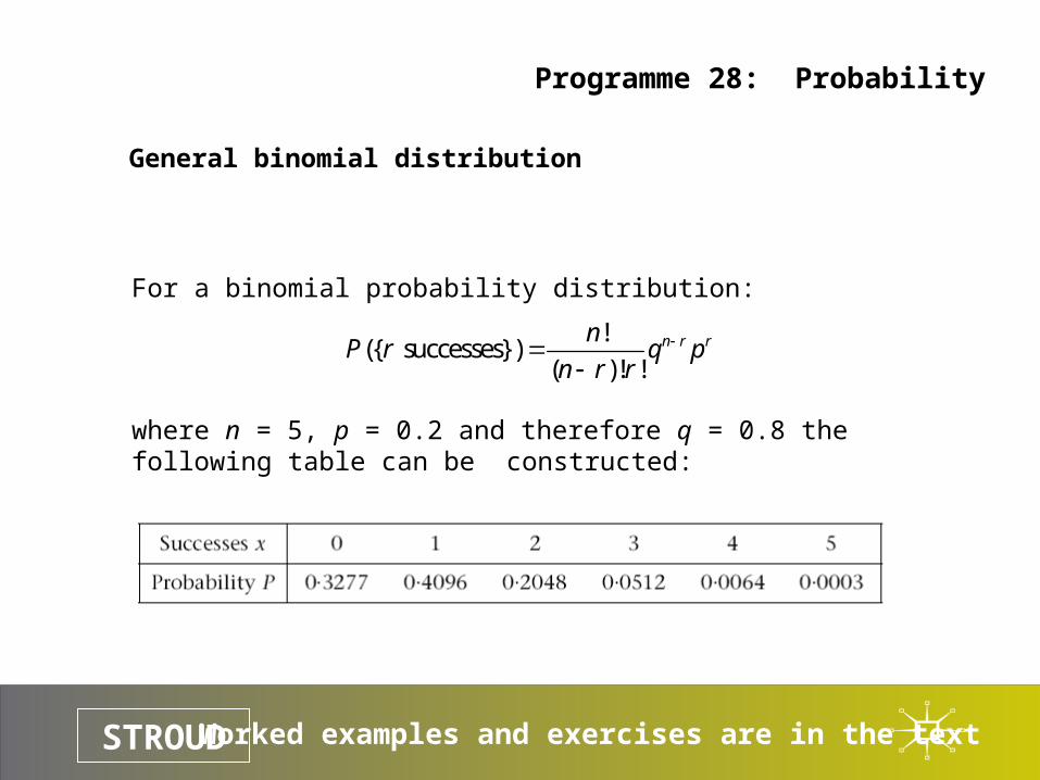
General binomial distribution
If a trial has two possible outcomes, success with a probability of p and failure with a probability of q then:
p + q = 1
In a sequence of n trials the probability of r successes is given by the general binomial term:
This distribution of probabilities is called the binomial probability distribution.
!({ successes})
( )! !n r rn
P r q pn r r
Worked examples and exercises are in the textSTROUD
Programme 28: Probability
General binomial distribution
For a binomial probability distribution:
where n = 5, p = 0.2 and therefore q = 0.8 the following table can be constructed:
!({ successes})
( )! !n r rn
P r q pn r r
Worked examples and exercises are in the textSTROUD
Programme 28: Probability
General binomial distribution
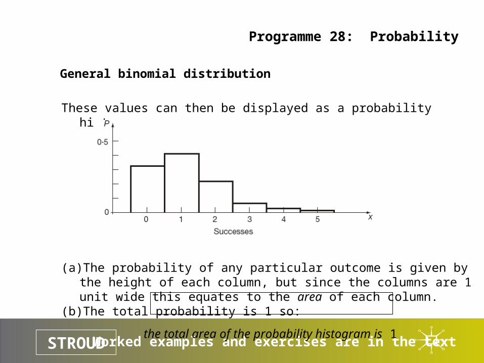
These values can then be displayed as a probability histogram:
(a) The probability of any particular outcome is given by the height of each column, but since the columns are 1 unit wide this equates to the area of each column.
(b) The total probability is 1 so:
the total area of the probability histogram is 1
Worked examples and exercises are in the textSTROUD
Programme 28: Probability
PART 2
Discrete probability distribution
Permutations and combinations
General binomial distribution
Mean and standard deviation of a probability distribution
The Poisson probability distribution
Continuous probability distributions
Standard normal curve
Worked examples and exercises are in the textSTROUD
Programme 28: Probability
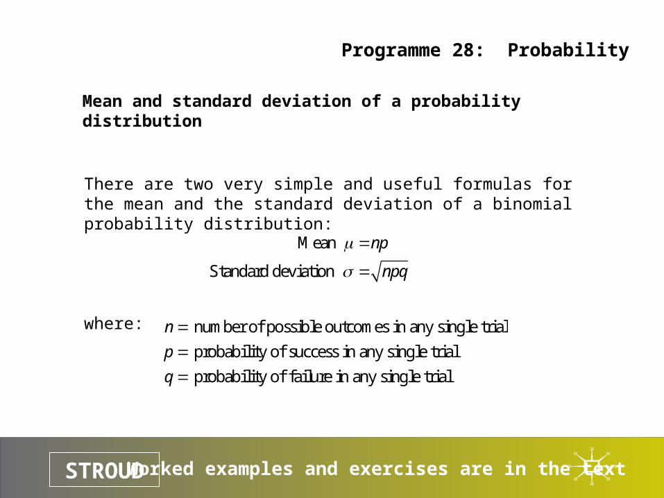
Mean and standard deviation of a probability distribution
There are two very simple and useful formulas for the mean and the standard deviation of a binomial probability distribution:
where:
Mean
Standard deviation
np
npq
number of possible outcomes in any single trial
probability of success in any single trial
probability of failure in any single trial
n
p
q
Worked examples and exercises are in the textSTROUD
Programme 28: Probability
PART 2
Discrete probability distribution
Permutations and combinations
General binomial distribution
Mean and standard deviation of a probability distribution
The Poisson probability distribution
Continuous probability distributions
Standard normal curve
Worked examples and exercises are in the textSTROUD
Programme 28: Probability
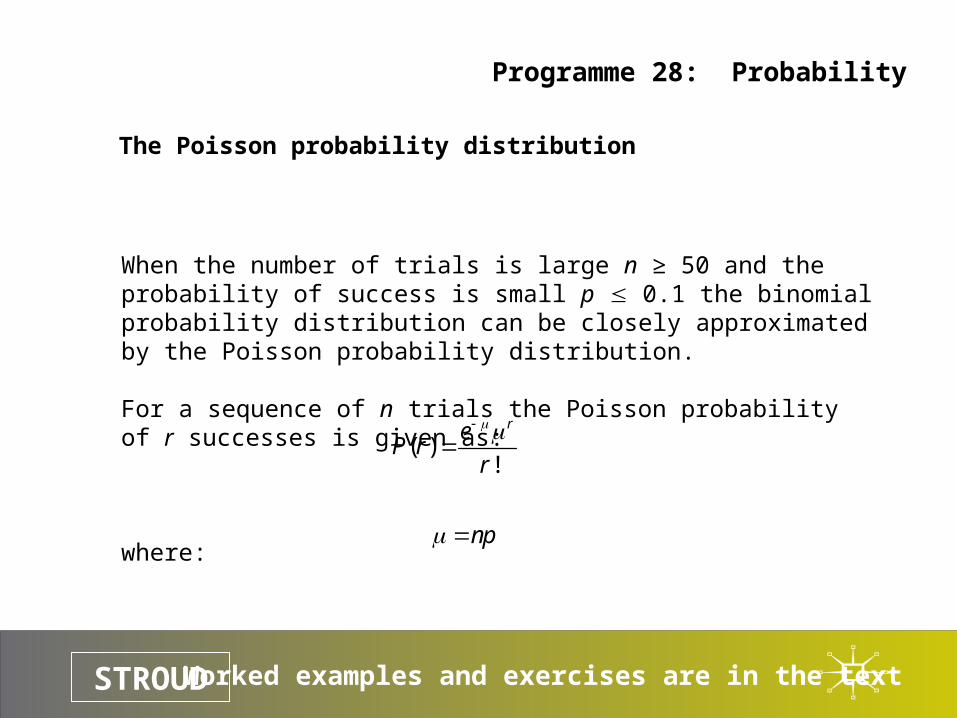
The Poisson probability distribution
When the number of trials is large n ≥ 50 and the probability of success is small p 0.1 the binomial probability distribution can be closely approximated by the Poisson probability distribution.
For a sequence of n trials the Poisson probability of r successes is given as:
where:
( )!
reP r
r
np
Worked examples and exercises are in the textSTROUD
Programme 28: Probability
PART 2
Discrete probability distribution
Permutations and combinations
General binomial distribution
Mean and standard deviation of a probability distribution
The Poisson probability distribution
Continuous probability distributions
Standard normal curve
Worked examples and exercises are in the textSTROUD
Programme 28: Probability
Continuous probability distributions
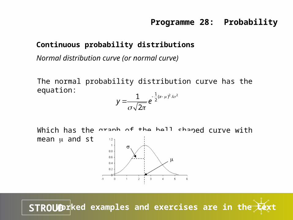
Normal distribution curve (or normal curve)
The binomial and Poisson probability distributions refer to discrete events.
Where continuous variables are involved the concern is one of finding the probability that a particular variable lies between certain limiting values.
For this reference is made to a continuous probability distribution – the normal probability distribution.
Worked examples and exercises are in the textSTROUD
Programme 28: Probability
Continuous probability distributions
Normal distribution curve (or normal curve)
The normal probability distribution curve has the equation:
Which has the graph of the bell shaped curve with mean and standard deviation
2 21( ) /
21
2
xy e
Worked examples and exercises are in the textSTROUD
Programme 28: Probability
PART 2
Discrete probability distribution
Permutations and combinations
General binomial distribution
Mean and standard deviation of a probability distribution
The Poisson probability distribution
Continuous probability distributions
Standard normal curve
Worked examples and exercises are in the textSTROUD
Programme 28: Probability
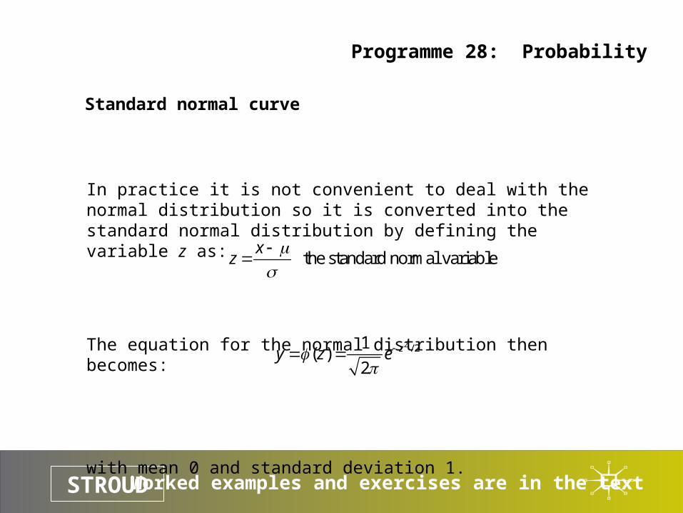
Standard normal curve
In practice it is not convenient to deal with the normal distribution so it is converted into the standard normal distribution by defining the variable z as:
The equation for the normal distribution then becomes:
with mean 0 and standard deviation 1.
the standard normal variablex
z
2 / 21( )
2zy z e
Worked examples and exercises are in the textSTROUD
Programme 28: Probability
Standard normal curve
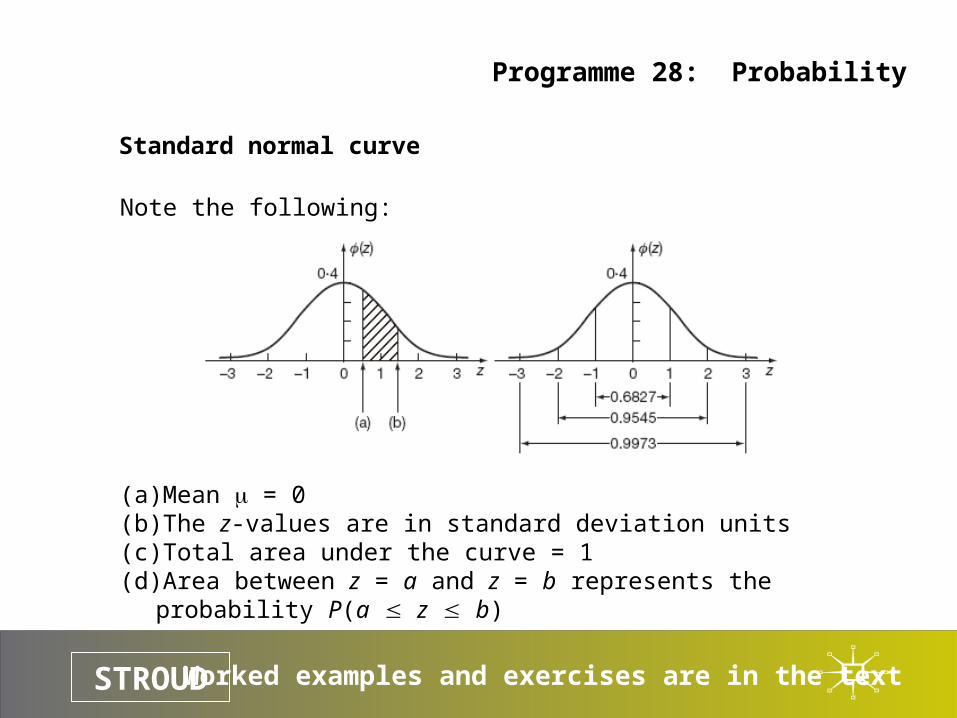
Note the following:
(a) Mean = 0(b) The z-values are in standard deviation units(c) Total area under the curve = 1(d) Area between z = a and z = b represents the probability P(a z b)
Worked examples and exercises are in the textSTROUD
Programme 28: Probability
Standard normal curve
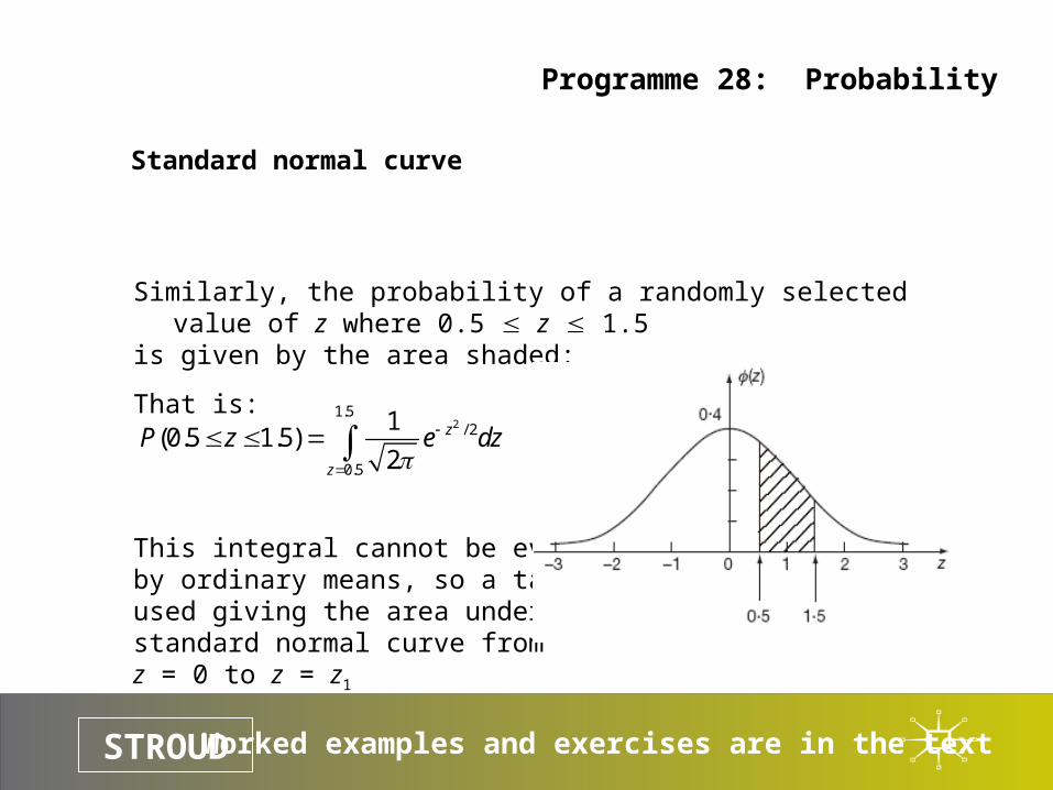
Similarly, the probability of a randomly selected value of z where 0.5 z 1.5is given by the area shaded:
That is:
This integral cannot be evaluated by ordinary means, so a table is used giving the area under the standard normal curve fromz = 0 to z = z1
21.5
/ 2
0.5
1(0.5 1.5)
2z
z
P z e dz
Worked examples and exercises are in the textSTROUD
Programme 28: Probability
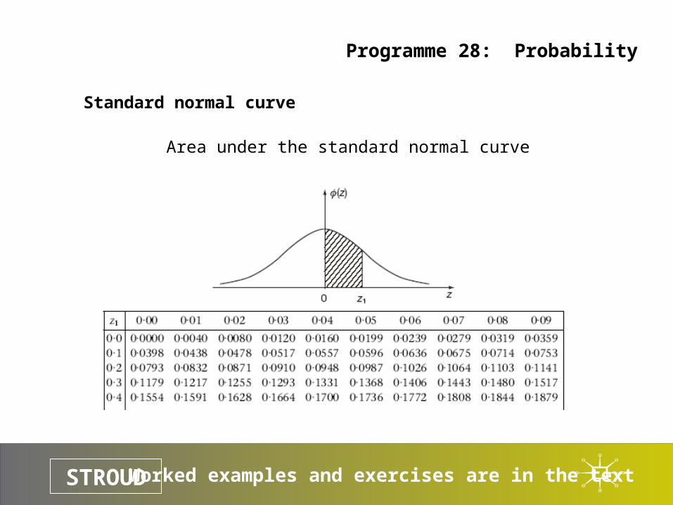
Standard normal curve
Area under the standard normal curve
Worked examples and exercises are in the textSTROUD
Learning outcomes
Understand the nature of probability as a measure of chance
Compute expectations of events from an experiment with a number of outcomes
Assign classical measures to the probability and be able to define the probabilities of both certainty and impossibility
Distinguish between mutually exclusive and mutually non-exclusive events and compute their probabilities
Compute conditional probabilities
Evaluate permutations and combinations
Use the binomial and Poisson probability distributions to calculate probabilities
Use the standard normal probability distribution to calculate probabilities
Programme 28: Probability