Worker Flows and Job Flows:A Quantitative Investigation∗

Shigeru Fujita† and Makoto Nakajima‡

This Version: May 2016

Abstract

This paper studies quantitative properties of a multiple-worker firm search/match-ing model and investigates how worker transition rates and job flow rates are inter-related. We show that allowing for job-to-job transitions in the model is essential tosimultaneously account for the cyclical features of worker transition rates and job flowrates. Important to this result are the distinctions between the job creation rate andthe hiring rate and between the job destruction rate and the layoff rate. In the modelwithout job-to-job transitions, these distinctions essentially disappear, thus making itimpossible to simultaneously replicate the cyclical features of both labor market flows.

Keywords: job flows, worker flows, multiple-worker firm, and search and matchingJEL Classification: E24, E32, J63, J64

∗We thank the anonymous referees, the editor (Gianluca Violante), and participants at many semi-nars and conferences for their comments and suggestions. The views expressed in this paper are those ofthe authors and do not necessarily reflect the views of the Federal Reserve Bank of Philadelphia or theFederal Reserve System. This paper is available free of charge at www.philadelphiafed.org/research-and-data/publications/working-papers.†Research Department, Federal Reserve Bank of Philadelphia. Ten Independence Mall, Philadelphia, PA

19106. E-mail: shigeru.fujita@phil.frb.org.‡Research Department, Federal Reserve Bank of Philadelphia. Ten Independence Mall, Philadelphia, PA

19106. E-mail: makoto.nakajima@phil.frb.org.

1

1 Introduction

The flow analysis is now a standard tool to analyze the labor market dynamics. Measuresof job creation and destruction rates, proposed by Davis et al. (1996), are constructed fromestablishment-level employment observations and are supposed to capture rates at whichnew jobs are created and existing jobs are destroyed. Cyclical features of these variableshave been extensively studied and are well known. For example, the job creation rate is pro-cyclical, while the job destruction rate is countercyclical. Worker transition rates, measuredfrom a survey of households, capture similar but distinct labor market information. Again,researchers have studied their cyclical features and find that the job finding rate for unem-ployed workers is procyclical and the separation rate into unemployment is countercyclical.

The macro-labor literature has used either job flow rates or worker transition rates asa yardstick to evaluate quantitative performance of labor search/matching models. Forexample, Mortensen and Pissarides (1994) and den Haan et al. (2000) focus on job flow ratesin evaluating their models’ quantitative performance. Since an influential paper by Shimer(2005), however, the literature has focused mostly on the model’s performance in replicatingthe cyclical features of worker transition rates.

In this paper, we consider both job flow rates and worker transition rates simultaneouslywithin one framework. As mentioned above, the overall empirical regularities of these dataare well established and tell us intuitive stories about what is happening in the labor market.For example, a higher job destruction rate is likely to imply the deterioration of the labormarket. A similar story can be told when the transition rate from employment to unem-ployment spikes up. As we will show in this paper, however, the relationships between theseflow variables are more complex and richer than these casual observations suggest. There-fore, there is much to learn from considering both flow measures simultaneously, and thesimultaneous analysis allows us to disentangle different underlying forces at work in drivingeach of these variables, thereby giving us a richer and better understanding of the U.S. labormarket dynamics.

For the purpose of this paper, we consider a search/matching model in which each firmoperates a decreasing returns-to-scale production technology and is subject to aggregate aswell as idiosyncratic productivity shocks. Each firm hires multiple workers, in contrast tothe canonical matching model of Mortensen and Pissarides (1994), in which a worker-firmmatch is taken to be the unit of analysis. Cooper et al. (2007) and Elsby and Michaels (2013)also study the multiple-worker firm environment. Our paper is different from these existingpapers because we explicitly incorporate job-to-job transitions into the model. Both themultiple-worker firm environment and job-to-job transitions are essential for analyzing bothworker transition rates and job flow rates. To see this point, note that job flows are defined byestablishment-level net employment changes over a quarterly period: Job creation aggregatesnet employment changes at the establishments that are expanding on net over the period,and, similarly, job destruction is the sum of net employment losses. To be consistent withthe measurement, we need a model with a meaningful notion of the establishment that hiresmany workers. Furthermore, in the environment in which job-to-job transitions are assumedaway, the difference between net employment changes and gross worker flows is largely futile

2

except for the difference that arises to due to the different data collection frequency.1 As asimple example, consider a firm that plans to expand its employment in the current period.In the absence of worker turnover due to quits, the number of hires is identical to net jobscreated in this period. However, job-to-job transitions introduce endogenous worker turnoverand thus work as a wedge between gross hires and net employment gains. The firm maylose some of its workers to other firms and thus net employment gains would differ fromgross hires. Importantly, the pace of job-to-job transitions in the model is time varying andthus the wedge is also time varying. In the paper, we analyze various cases in which netemployment changes and gross flows are different.

We calibrate the model by matching the steady-state levels of worker transition ratesand cross-sectional moments such as the dispersion of the employment growth distributionreported by Davis et al. (2010). We show that the calibrated model captures essential fea-tures of the cross-sectional “hockey stick” relationships between gross worker flows and netemployment growth studied by Davis et al. (2012). We show that the model successfullyreplicates overall cyclical features of worker transition rates and the job creation and de-struction rates. As noted above, incorporating job-to-job transitions into the model playsa crucial role for this result. Suppose that the firm aims to reduce its workforce size. Howmany workers the firm aims to lay off depends on how many workers quit the firm. Thosewho are laid off flow into unemployment, while those who quit make job-to-job transitions,implying that the transition rate from employment to unemployment (EU transition rate)is different from the job destruction rate. It is also possible that this firm actually hiressome workers when the number of quits exceeds the total number of desired reduction ofemployment. The relationship between the job creation rate (sum of net employment gainsnormalized by aggregate employment) and the overall hiring rate (all hires normalized byaggregate employment) is even more complex. As discussed previously, the presence of job-to-job transitions makes net employment change and gross hires different from each other.There is an important aggregate implication of this fact. Suppose (for the sake of an illus-tration) that one expanding firm hires all new workers from another expanding firm. In thiscase, the latter expanding firm must be hiring more workers than it lost to “create new jobs.”If, on the other hand, those two firms hire all of their new workers from the unemploymentpool or shrinking firms, net job gains are equal to total hires. These examples imply thatthe relationship between net job gains and total hires depends on the pace of job-to-jobtransitions and the share of job-to-job transitions that occur within expanding firms, bothof which are endogenously changing over time along with the aggregate shock.

Moreover, the example in the previous paragraph shows how a chain of hiring occurswhen workers make job-to-job transitions from one expanding firm to other expanding firms.That is, as the pace of job-to-job transitions increases, the number of new hires necessary toachieve the target employment size increases. We show that the chain of hiring is reflectedin the behavior of vacancies in our model in which vacancies are more procyclical, volatile,

1Job flows are measured by net employment changes over a quarterly period, whereas worker transitionrates are measured from the monthly survey. We address this issue by solving the model at monthly frequencyand analyzing job flows constructed in the same way as in the actual data.

3

and persistent compared with the behavior in the model without job-to-job transitions. Theresult in our model captures the notion of “vacancy chain” introduced by Akerlof et al.(1988).

Let us now discuss where our paper stands in relation to the literature. As mentionedabove, this paper is closely related to the studies by Cooper et al. (2007) and Elsby andMichaels (2013), who also quantitatively analyze a multiple-worker firm matching model.The key difference from these papers is the presence of job-to-job transitions in our model.There are several other papers that study the directed search environment with decreasingreturns to scale (e.g., Kaas and Kircher (2013) and Schaal (2012)). Kaas and Kircher analyzethe environment without job-to-job transitions, and Schaal adds on-the-job search to themodel. However, Schaal focuses more on the recent Great Recession episode in the presence ofthe uncertainty shock. On the other hand, our paper follows the random matching traditionmore closely and looks more generally at the model’s cyclical features.2

In terms of economic interest, our paper is related to the work by Mortensen (1994), whoalso attempts to explain the cyclicality of worker transition rates and job flow rates. However,he explores this topic in a single-worker firm matching model with on-the-job search, andthus faces the limitations we discussed above. Veracierto (2009) provides a synthesis ofthe different strands of literature (in particular, the Mortensen-Pissarides random-matchingframework and the Lucas and Prescott (1974) island framework) and discusses the cyclicalproperties of worker transition rates and job flow rates in the model. However, his modeldoes not allow for job-to-job transitions. Our analysis of the relationships between workertransition rates and job flow rates is a key part of our paper that is distinct from his paper.3

This paper proceeds as follows. In the next section, we summarize the business cyclefeatures of worker transition rates and job flow rates. Section 3 presents our model. Section 4summarizes the solution algorithms to numerically solve the model. The details are presentedin the Appendix. Section 5 discusses the calibration. Section 6 discusses the paper’s mainresults. To demonstrate the importance of job-to-job transitions in our model, we comparethe performance of our model with that of the model without job-to-job transitions. Thefinal section concludes by discussing some limitations of our paper.

2 Empirical Facts

This section reviews the cyclical properties of worker transition rates and job flow rates.While one can find the cyclical properties of these series in the literature, the two sets ofdata are usually discussed in isolation. Let us first review the definitions of the series.

2A recent work by Moscarini and Postel-Vinay (2013) analyzes and solves the random-matching, wage-posting model under the presence of the aggregate shock. But worker transitions into unemployment areexogenous, and their research interest is different from ours.

3Note, however, that his model is a full-fledged real business cycle model with physical capital and riskaversion. He can therefore assess the broader macroeconomic implications of this model. See also Veracierto(2007), who studies normative aspects of a similar environment without aggregate uncertainty.

4

2.1 Measurement

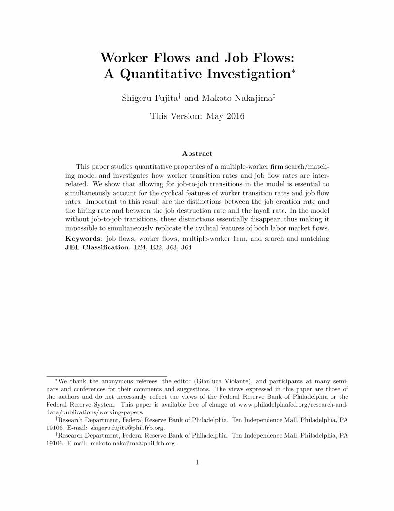
Job flow rates. The job flow series are measured from the Business Employment Dynamics(BED) data, which are based on the administrative records of the Quarterly Census ofEmployment and Wages (QCEW).4 These measures were originally developed by Davis et al.(1996): Job creation (destruction) is defined as the sum of net employment gains (losses)over all establishments that expand (contract) or start up (shut down) between the twosampling dates. Because we are interested in business cycle fluctuations of the series, weuse the series that trace net employment changes over a quarterly period. Normalizingcreation and destruction by aggregate employment yields job creation and destruction rates,respectively.5 In this paper, we sometimes use the term “job flows” as a generic term, butthe specific empirical measures we aim to explain are always job flow rates. The sampleperiod of the series starts at 1992Q3 and ends at 2011Q4.

Worker transition rates. We use the Current Population Survey (CPS) to measureworker transition rates. The CPS asks whether the worker is employed and, if nonemployed,whether he or she is engaged in active job search activities (i.e., unemployed) during thepreceding month. While the CPS is designed to provide a snapshot of the U.S. labor marketfor each month, one can use its longitudinal component to obtain measures of worker flows.We use the series constructed by the BLS.6 Worker transition rates between employmentand unemployment are, respectively, measured by:

EUtEt−1

andUEtUt−1

, (1)

where EUt (UEt) refers to the number of workers who switch their labor market statusfrom “employed” (“unemployed”) to “unemployed” (“employed”) between month t− 1 andt. EUt and UEt represent separations into unemployment and hires from unemployment,respectively. The definitions in Equation (1) give the EU transition rate and UE transitionrate, respectively. The sample period for the BLS data is from January 1990 to December2011.7

We also consider the job-to-job transition rate. Measuring job-to-job transitions in theCPS became feasible after the CPS redesign in 1994. Specifically, the dependent coding,which asks the individual if he or she is currently employed by the same employer as in theprevious month, made it possible to measure the number of job-to-job movers. Fallick andFleischman (2004) are the first to exploit this data structure for measuring the job-to-job

4The BED series are available at www.bls.gov/bdm.5More precisely, average employment between the beginning and the end of the quarter is used for

normalization.6The data are available at www.bls.gov/cps/cps flows.htm. Fujita and Ramey (2006) also construct flow

series that are comparable to the BLS series. The cyclicality of the two data sets is very similar. See Fujitaand Ramey (2006) for the data construction details and measurement issues in the CPS.

7In the BLS data, the flow that occurs from t − 1 and t is dated at t. Using that convention, the BLSflow data start at February 1990.

5

0.01

0.02

0.03

0.04

0.05

0.06

0.07

0.08

0.09

1993 1994 1995 1996 1997 1998 1999 2000 2001 2002 2003 2004 2005 2006 2007 2008 2009 2010 2011

Total creation rateExpansion rate

Entry rateTotal destruction rate

Contraction rateExit rate

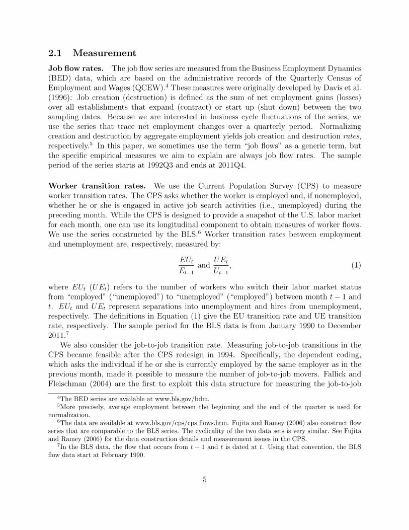
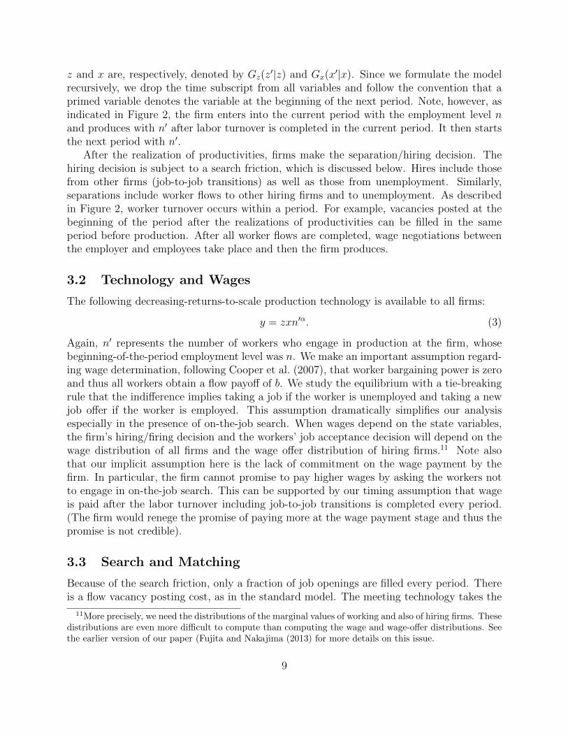
Figure 1: Job Creation and Destruction RatesNotes: The data are taken from the BLS Business Employment Dynamics and coverthe private business sector.

transition rate in the CPS.8 Denoting the number of workers who are employed at differentemployers between t− 1 and t by EEt, we can write the job-to-job transition rate as

EEtEt−1

. (2)

The Fallick-Fleischman data are updated regularly and the sample period for our analysisis from January 1994 to December 2011. All monthly transition rates are converted intoquarterly series by time averaging.

2.2 Business Cycle Statistics

Unimportance of entry and exit. First, consider Figure 1, where we plot the time seriesof job flow rates. The figure shows not only the total rates of job creation and destructionbut also their breakdowns into expansion, entry, contraction, and exit. The intention is toshow the unimportance of the extensive margins for the business cycle fluctuations of jobflow rates. According to the data, roughly 75% of total job flows come from expansion orcontraction of the existing establishments at a quarterly frequency. More important, cyclicalfluctuations of job flow rates are mostly accounted for by expansion or contraction: Thecorrelation between the total job creation (destruction) rate and the expansion (contraction)rate is higher than 0.95. It is important to recognize that these two facts do not imply the

8Moscarini and Thompson (2007) explore several measurement issues of the CPS-based job-to-job tran-sition rate and correct some measurement issues that existed in Fallick and Fleischman (2004). While theiradjustments alter the overall level of the job-to-job transition rate somewhat, the time-series behavior is notsignificantly affected. We thus use the readily available series by Fallick and Fleischman (2004).

6

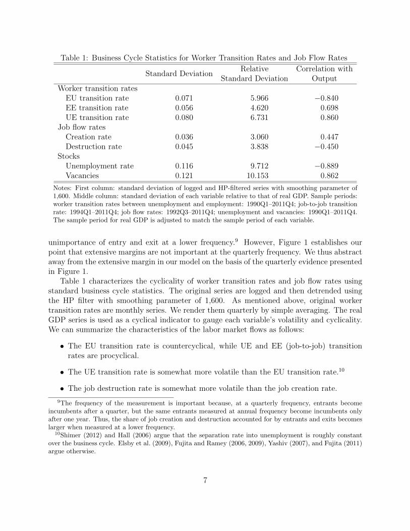
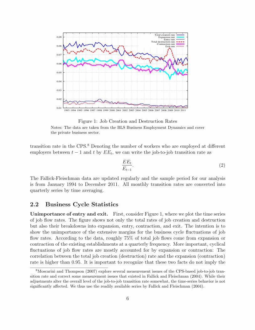
Table 1: Business Cycle Statistics for Worker Transition Rates and Job Flow Rates

Standard DeviationRelative Correlation with

Standard Deviation OutputWorker transition rates

EU transition rate 0.071 5.966 −0.840EE transition rate 0.056 4.620 0.698UE transition rate 0.080 6.731 0.860

Job flow ratesCreation rate 0.036 3.060 0.447Destruction rate 0.045 3.838 −0.450

StocksUnemployment rate 0.116 9.712 −0.889Vacancies 0.121 10.153 0.862

Notes: First column: standard deviation of logged and HP-filtered series with smoothing parameter of1,600. Middle column: standard deviation of each variable relative to that of real GDP. Sample periods:worker transition rates between unemployment and employment: 1990Q1–2011Q4; job-to-job transitionrate: 1994Q1–2011Q4; job flow rates: 1992Q3–2011Q4; unemployment and vacancies: 1990Q1–2011Q4.The sample period for real GDP is adjusted to match the sample period of each variable.

unimportance of entry and exit at a lower frequency.9 However, Figure 1 establishes ourpoint that extensive margins are not important at the quarterly frequency. We thus abstractaway from the extensive margin in our model on the basis of the quarterly evidence presentedin Figure 1.

Table 1 characterizes the cyclicality of worker transition rates and job flow rates usingstandard business cycle statistics. The original series are logged and then detrended usingthe HP filter with smoothing parameter of 1,600. As mentioned above, original workertransition rates are monthly series. We render them quarterly by simple averaging. The realGDP series is used as a cyclical indicator to gauge each variable’s volatility and cyclicality.We can summarize the characteristics of the labor market flows as follows:

• The EU transition rate is countercyclical, while UE and EE (job-to-job) transitionrates are procyclical.

• The UE transition rate is somewhat more volatile than the EU transition rate.10

• The job destruction rate is somewhat more volatile than the job creation rate.

9The frequency of the measurement is important because, at a quarterly frequency, entrants becomeincumbents after a quarter, but the same entrants measured at annual frequency become incumbents onlyafter one year. Thus, the share of job creation and destruction accounted for by entrants and exits becomeslarger when measured at a lower frequency.

10Shimer (2012) and Hall (2006) argue that the separation rate into unemployment is roughly constantover the business cycle. Elsby et al. (2009), Fujita and Ramey (2006, 2009), Yashiv (2007), and Fujita (2011)argue otherwise.

7

(x, n, z,m) (x′, n′, z′,m′)

Beginning ofthe current period

Beginning ofthe next period

ProductionBargaining

New (x′, z′) drawnFirmschoose n′

Firms loseworkers throughjob-to-job transition

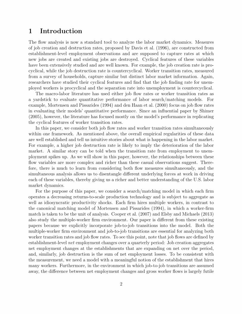
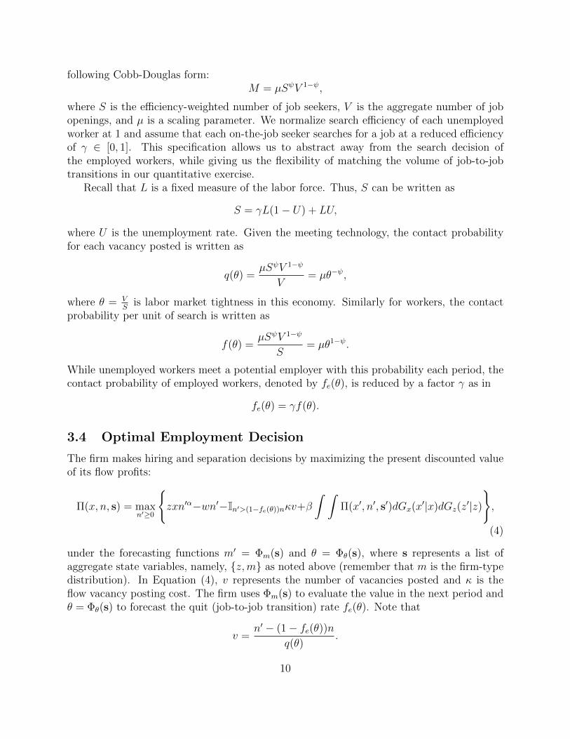
Figure 2: Timing of Events

• The job destruction rate is countercyclical and the job creation rate is procyclical.But the correlations with output are weaker in general than those of worker transitionrates.

The fact that the correlations of job flow rates are weaker than those of worker transitionrates is an important observation because it implies that those measures are not as robustas worker transition rates as business cycle indicators. We show that the same pattern holdsin our model as well and we explore the underlying reasons for this observation.

Table 1 also shows volatilities of the unemployment rate and vacancies. As is well knownin the literature, these two variables are quite volatile when compared with the volatility oflabor productivity. The same is true with respect to output volatility. Lastly, a well-knownfact about the cyclicality of unemployment and vacancies, i.e., the Beveridge curve, can alsobe observed from each variable’s correlation with output.

3 Model

Our model is similar to the ones developed by Cooper et al. (2007) and Elsby and Michaels(2013). Time is discrete. There are two types of agents: firms and workers. Both areinfinitely lived and risk neutral. The total measure of firms is normalized to one. The totalmeasure of workers is denoted by L.

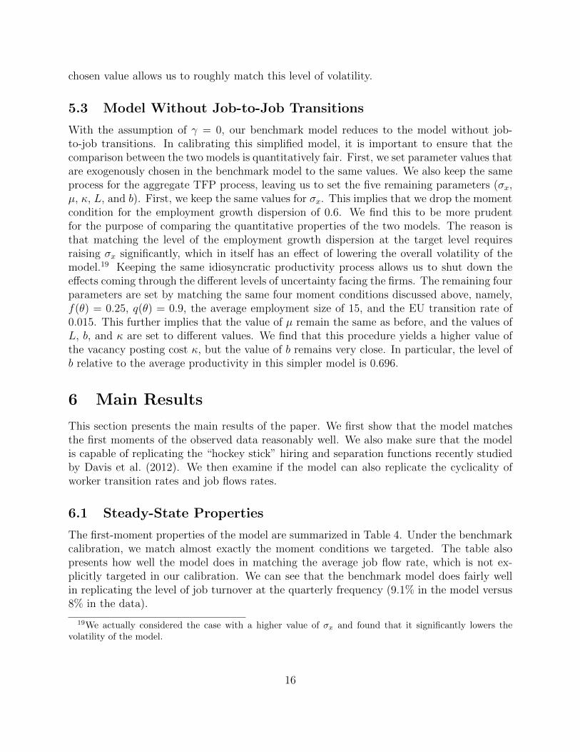
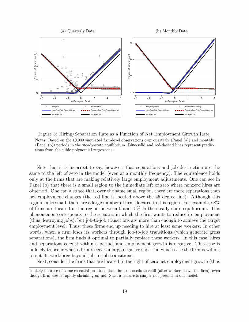
3.1 Timing

The timing of events is summarized in Figure 2. At the beginning of each period, a firm’sidiosyncratic states are characterized by (x, n), where x represents idiosyncratic productivityand n represents the number of its workers. In addition, there is aggregate uncertainty in theeconomy in the form of a shock to aggregate productivity z. As will be clear later, each firm’sdecision is also influenced by the economy wide joint distribution of x and n and is writtenas m(x, n). We summarize the aggregate states by s = {z,m}. The stochastic processes for

8

z and x are, respectively, denoted by Gz(z′|z) and Gx(x

′|x). Since we formulate the modelrecursively, we drop the time subscript from all variables and follow the convention that aprimed variable denotes the variable at the beginning of the next period. Note, however, asindicated in Figure 2, the firm enters into the current period with the employment level nand produces with n′ after labor turnover is completed in the current period. It then startsthe next period with n′.

After the realization of productivities, firms make the separation/hiring decision. Thehiring decision is subject to a search friction, which is discussed below. Hires include thosefrom other firms (job-to-job transitions) as well as those from unemployment. Similarly,separations include worker flows to other hiring firms and to unemployment. As describedin Figure 2, worker turnover occurs within a period. For example, vacancies posted at thebeginning of the period after the realizations of productivities can be filled in the sameperiod before production. After all worker flows are completed, wage negotiations betweenthe employer and employees take place and then the firm produces.

3.2 Technology and Wages

The following decreasing-returns-to-scale production technology is available to all firms:

y = zxn′α. (3)

Again, n′ represents the number of workers who engage in production at the firm, whosebeginning-of-the-period employment level was n. We make an important assumption regard-ing wage determination, following Cooper et al. (2007), that worker bargaining power is zeroand thus all workers obtain a flow payoff of b. We study the equilibrium with a tie-breakingrule that the indifference implies taking a job if the worker is unemployed and taking a newjob offer if the worker is employed. This assumption dramatically simplifies our analysisespecially in the presence of on-the-job search. When wages depend on the state variables,the firm’s hiring/firing decision and the workers’ job acceptance decision will depend on thewage distribution of all firms and the wage offer distribution of hiring firms.11 Note alsothat our implicit assumption here is the lack of commitment on the wage payment by thefirm. In particular, the firm cannot promise to pay higher wages by asking the workers notto engage in on-the-job search. This can be supported by our timing assumption that wageis paid after the labor turnover including job-to-job transitions is completed every period.(The firm would renege the promise of paying more at the wage payment stage and thus thepromise is not credible).

3.3 Search and Matching

Because of the search friction, only a fraction of job openings are filled every period. Thereis a flow vacancy posting cost, as in the standard model. The meeting technology takes the

11More precisely, we need the distributions of the marginal values of working and also of hiring firms. Thesedistributions are even more difficult to compute than computing the wage and wage-offer distributions. Seethe earlier version of our paper (Fujita and Nakajima (2013) for more details on this issue.

9

following Cobb-Douglas form:M = µSψV 1−ψ,

where S is the efficiency-weighted number of job seekers, V is the aggregate number of jobopenings, and µ is a scaling parameter. We normalize search efficiency of each unemployedworker at 1 and assume that each on-the-job seeker searches for a job at a reduced efficiencyof γ ∈ [0, 1]. This specification allows us to abstract away from the search decision ofthe employed workers, while giving us the flexibility of matching the volume of job-to-jobtransitions in our quantitative exercise.

Recall that L is a fixed measure of the labor force. Thus, S can be written as

S = γL(1− U) + LU,

where U is the unemployment rate. Given the meeting technology, the contact probabilityfor each vacancy posted is written as

q(θ) =µSψV 1−ψ

V= µθ−ψ,

where θ = VS

is labor market tightness in this economy. Similarly for workers, the contactprobability per unit of search is written as

f(θ) =µSψV 1−ψ

S= µθ1−ψ.

While unemployed workers meet a potential employer with this probability each period, thecontact probability of employed workers, denoted by fe(θ), is reduced by a factor γ as in

fe(θ) = γf(θ).

3.4 Optimal Employment Decision

The firm makes hiring and separation decisions by maximizing the present discounted valueof its flow profits:

Π(x, n, s) = maxn′≥0

{zxn′α−wn′−In′>(1−fe(θ))nκv+β

∫ ∫Π(x′, n′, s′)dGx(x

′|x)dGz(z′|z)

},

(4)

under the forecasting functions m′ = Φm(s) and θ = Φθ(s), where s represents a list ofaggregate state variables, namely, {z,m} as noted above (remember that m is the firm-typedistribution). In Equation (4), v represents the number of vacancies posted and κ is theflow vacancy posting cost. The firm uses Φm(s) to evaluate the value in the next period andθ = Φθ(s) to forecast the quit (job-to-job transition) rate fe(θ). Note that

v =n′ − (1− fe(θ))n

q(θ).

10

Observe that the firm loses fe(θ)n workers through job-to-job transitions. As in Elsby andMichaels (2013), the optimal employment decision of the firm is characterized by an (s, S)rule, with the inaction region (n∗, n∗) characterized by the following first-order conditions:

αzxn∗α−1 − w − κ

q(θ)+ β

∫ ∫Πn(x′, n∗, s′)dGx(x

′|x)dGz(z′|z) = 0, (5)

αzxn∗α−1 − w + β

∫ ∫Πn(x′, n∗, s′)dGx(x

′|x)dGz(z′|z) = 0. (6)

The envelope conditions are written as

Πn(x, n, s) =

κ1−fe(θ))

q(θ)if n < n∗,

(1− fe(θ))[αzxn′α−1 − w + β

∫ ∫Πn(x′, n, s′)dGxdGz

]if n ∈ [n∗, n∗],

0 if n > n∗,(7)

where n = (1−fe(θ))n. Relative to Cooper et al. (2007) and Elsby and Michaels (2013), thekey difference is that the pace of the job-to-job transitions at the firm depends on endogenousaggregate state variable θ. When fe(θ) is high, the firm knows that more workers will leavethe firm. Thus, for example, if the firm would like to expand its employment size, it needsto hire more workers to expand its size on net.

3.5 Equilibrium

The equilibrium of the model economy with the aggregate shock consists of the value functionΠ(x, n, s), the employment decision rule g(x, n, s), the wage function w = b, and the fore-casting functions for the type distribution m′ = Φm(s) and labor market tightness θ = Φθ(s),such that (i) g(x, n, s) maximizes the value of the firm and Π(x, n, s) is the associated op-timal value function; and (ii) the forecasting functions Φm(s) and Φθ(s) are consistent withthe optimal employment decision of the individual firms. Note that Φm and Φθ are unknownfunctions of the aggregate state variables including the type distribution m. We capture theinformation in the distribution by the mean as discussed below.

4 Computation

The details of the computational algorithms are presented in the Appendix. To ease thenotation, let us define the expected marginal profit function after the employment decisionis completed in the current period as

D(x, n′, z,m′) =

∫ ∫Πn(x′, n′, z′,m′)dGx(x

′|x)dGz(z′|z). (8)

To approximate this function, we replace the type distribution m by the aggregate unemploy-ment rate U .12 The idea is the same as the solution technique used to solve heterogeneous

12Note that we approximate the expected value function D(.) instead of Πn(.) since the former is smootherthan the latter.

11

agent models with the uninsurable income risk, where the information in the wealth dis-tribution is captured well with its mean. The D function is approximated by a piecewiselinear function of the continuous state variables n′, z, and U for each discretized value ofidiosyncratic productivity x.

4.1 Steady-State Equilibrium

In the steady-state equilibrium, the aggregate state variable s is time-invariant and thus canbe dropped. The first stage to solve for this equilibrium is to iterate on n∗(x, n), n∗(x, n),and D(x, n′) for a given guess of market tightness θ, using the first-order conditions (5) and(6).13

Once we obtain the convergence on the optimal employment adjustment function n′ =g(x, n) and the D(x, n′) function, the second stage of the algorithm simulates the economyto obtain the invariant distribution of m(x, n). Using this invariant type distribution, weobtain the aggregate labor market variables, such as vacancies posted, the number of jobseekers, and thus market tightness. The entire process repeats until the convergence onthe employment policy function, the expected marginal profit function D(x, n′), and markettightness is completed.

4.2 Dynamic Stochastic Equilibrium

In the presence of aggregate uncertainty, current-period market tightness θ depends not onlyon realized aggregate productivity z but also on the type distribution m(x, n). In making theemployment adjustment decision, each firm therefore needs to know the relationship betweenθ and m(x, n) as well as z. As mentioned above, it is assumed that the firms use only themean of the distribution (aggregate employment and thus equivalently unemployment U) tosummarize the information in m(x, n), following the methodology often used in models ofuninsurable income risk (e.g., Krusell and Smith (1998)). Further, calculating and updatingthe D(x, n′, z,m′) function requires the firms to form the forecast for the next-period typedistribution. Given our assumption about the approximate equilibrium, this entails fore-casting next-period aggregate unemployment, U ′, using current-period unemployment andrealized aggregate productivity.

The algorithm starts with guessing a set of coefficients of the forecasting rules. Giventhese rules, we can solve for each individual firm’s problem, following the procedure usedto solve for the steady-state equilibrium (except that those functions now depend on theaggregate state variables). Once we achieve the convergence on the D(x, n′, z, U ′) functionand the employment policy function g(x, n, z, U), we simulate a large panel data set fromwhich we can obtain a long time series of {z, U, θ}. By using these objects, we can updatethe forecasting rules by running OLS regressions. The algorithm stops when the convergenceon the coefficients of the forecasting rules is achieved.

13Strictly speaking, n∗(x, n) actually does not depend on n, but we are using more general notation here.

12

Table 2: Model Parameters

Symbol Descriptionψ Elasticity of matching function with respect to job seekersα Curvature of the production functionβ Time discount factorµ Scale parameter of the matching functionκ Vacancy posting costγ Search intensity of on-the-job seekersb Flow outside benefitρx Persistence of the idiosyncratic productivity processσx Standard deviation of the idiosyncratic shockρz Persistence of the aggregate productivity processσz Standard deviation of the aggregate shockL Labor force (population) size

5 Calibration

One period in the model is assumed to be one month. The exogenous productivity processesfollow the standard AR(1) processes:

ln z′ = ρz ln z + ε′z,

lnx′ = ρx lnx+ ε′x,

where εx ∼ N(0, σ2x) and εz ∼ N(0, σ2

z). These processes are then approximated by a finite-state, first-order Markov chain.14

Note that some of the statistics used to calibrate the model are available only at quarterlyfrequency or annual frequency. In particular, job flow rates are measured by taking netemployment changes over a quarterly period and it is important for us to construct themodel-based statistics in the same way as in the observed data. The details are discussedbelow.

We partition the model parameters into two groups: the one determined exogenously tothe model without solving the model and the other determined by matching the empiricalmoments. Table 2 provides the summary of the model parameters.

5.1 Parameters Set Exogenously

First, the time discount factor β is set to 0.996, which implies the quarterly discount factor of0.99, a standard value used in the business cycle literature. The curvature of the production

14While we use the finite-state approximation in calculating the conditional expectation with respect toaggregate uncertainty (when we solve the firm’s problem), we maintain the original AR(1) process in thesimulation stage so that the process has a continuous state space. This enables us to generate the smoothimpulse response functions presented below.

13

function α is set to 0.72. This appears to be a value commonly used in the literature, forexample, by Cooper et al. (2007). We also considered a lower value (0.67) and found that thequantitative results were hardly affected. The elasticity of the matching function with respectto unemployment 1− ψ are set to 0.5. The persistence parameter of aggregate productivityis set to 0.983, which implies a quarterly autocorrelation of 0.95, following the convention ofthe business cycle literature. The persistence parameter of idiosyncratic productivity is setto 0.95. It is chosen to be fairly persistent following the literature. We also experimentedwith different values (such as 0.99 and 0.90) and found that the results were insensitive withrespect to these alternative values.

5.2 Parameters Set Endogenously

The remaining seven parameters are set by matching the seven moment conditions. For thepurpose of clarity, we describes the procedure by associating one particular parameter withone moment condition that is most useful for the identification. In truth, however, eachparameter cannot be set separately and thus our procedure should be considered as jointlyminimizing the distance between the model-based moments and corresponding empiricalmoments.

First, we use the scale parameter of the matching function µ and the vacancy postingcost κ to achieve the average levels of the monthly UE transition rate f(θ) and job fillingrate q(θ) at 0.25 and 0.9, respectively. The former number is based on the time-series dataon the UE transition rate computed from the CPS labor flow data for the period January1990 through December 2011.15 The latter is based on the evidence by Davis et al. (2013),who show that the daily job filling rate fluctuates at around 7%, which translates into themonthly filling rate of 0.9.16 We set µ at 0.474 and κ at 0.269 to hit these targets as closelyas possible.

The search intensity parameter of employed workers γ is selected to match the averagejob-to-job transition rate in the Fallick and Fleischman (2004) data that cover the periodbetween January 1994 and December 2011. The average job-to-job transition rate over thisperiod is around 2.5% in the data. Remember that we target the monthly UE transitionrate f(θ) at 0.25. Thus, γ = 0.1 allows us to match the job-to-job transition rate of 2.5%.

Next, we calibrate the standard deviation of the shock to firm-level productivity σx by re-ferring to the dispersion of the employment growth distribution. Davis et al. (2007) calculateemployment-weighted cross-sectional dispersion (standard deviation) of annual employmentgrowth rates using the Longitudinal Business Database (LBD) for the period 1978 through2001. Their figure shows that the standard deviation fluctuates roughly around 0.60. Ourmodel generates a value close to this target with σx = 0.078. Note that the empirical mea-sure is based on net employment changes over an annual interval. We therefore constructthe corresponding statistic in our model, taking net employment changes over 12 periods.

15Given that all employed workers accept outside offers (conditional on searching on the job, which isexogenously set by γ), the job finding rate of on-the-job seekers is identical to the one for unemployedworkers.

16Fujita and Ramey (2012) also use the same target value, based on the evidence by Barron et al. (1997).

14

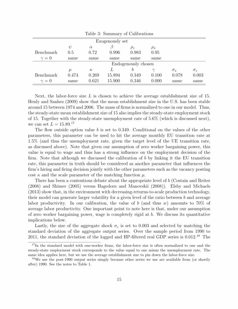
Table 3: Summary of Calibrations

Exogenously setψ α β ρz ρx

Benchmark 0.5 0.72 0.996 0.983 0.95γ = 0 same same same same same

Endogenously chosenµ κ L b γ σx σz

Benchmark 0.474 0.269 15.894 0.349 0.100 0.078 0.003γ = 0 same 0.621 15.900 0.346 0.000 same same

Next, the labor-force size L is chosen to achieve the average establishment size of 15.Henly and Sanhez (2009) show that the mean establishment size in the U.S. has been stablearound 15 between 1974 and 2006. The mass of firms is normalized to one in our model. Thus,the steady-state mean establishment size of 15 also implies the steady-state employment stockof 15. Together with the steady-state unemployment rate of 5.6% (which is discussed next),we can set L = 15.89.17

The flow outside option value b is set to 0.349. Conditional on the values of the otherparameters, this parameter can be used to hit the average monthly EU transition rate at1.5% (and thus the unemployment rate, given the target level of the UE transition rate,as discussed above). Note that given our assumption of zero worker bargaining power, thisvalue is equal to wage and thus has a strong influence on the employment decision of thefirm. Note that although we discussed the calibration of b by linking it the EU transitionrate, this parameter in truth should be considered as another parameter that influences thefirm’s hiring and firing decision jointly with the other parameters such as the vacancy postingcost κ and the scale parameter of the matching function µ.

There has been a contentious debate about the appropriate level of b (Costain and Reiter(2008) and Shimer (2005) versus Hagedorn and Manovskii (2008)). Elsby and Michaels(2013) show that, in the environment with decreasing-returns-to-scale production technology,their model can generate larger volatility for a given level of the ratio between b and averagelabor productivity. In our calibration, the value of b (and thus w) amounts to 70% ofaverage labor productivity. One important point to note here is that, under our assumptionof zero worker bargaining power, wage is completely rigid at b. We discuss its quantitativeimplications below.

Lastly, the size of the aggregate shock σz is set to 0.003 and selected by matching thestandard deviation of the aggregate output series. Over the sample period from 1990 to2011, the standard deviation of the logged and HP-filtered real GDP series is 0.012.18 The

17In the standard model with one-worker firms, the labor-force size is often normalized to one and thesteady-state employment stock corresponds to the value equal to one minus the unemployment rate. Thesame idea applies here, but we use the average establishment size to pin down the labor-force size.

18We use the post-1990 output series simply because other series we use are available from (or shortlyafter) 1990. See the notes to Table 1.

15

chosen value allows us to roughly match this level of volatility.

5.3 Model Without Job-to-Job Transitions

With the assumption of γ = 0, our benchmark model reduces to the model without job-to-job transitions. In calibrating this simplified model, it is important to ensure that thecomparison between the two models is quantitatively fair. First, we set parameter values thatare exogenously chosen in the benchmark model to the same values. We also keep the sameprocess for the aggregate TFP process, leaving us to set the five remaining parameters (σx,µ, κ, L, and b). First, we keep the same values for σx. This implies that we drop the momentcondition for the employment growth dispersion of 0.6. We find this to be more prudentfor the purpose of comparing the quantitative properties of the two models. The reason isthat matching the level of the employment growth dispersion at the target level requiresraising σx significantly, which in itself has an effect of lowering the overall volatility of themodel.19 Keeping the same idiosyncratic productivity process allows us to shut down theeffects coming through the different levels of uncertainty facing the firms. The remaining fourparameters are set by matching the same four moment conditions discussed above, namely,f(θ) = 0.25, q(θ) = 0.9, the average employment size of 15, and the EU transition rate of0.015. This further implies that the value of µ remain the same as before, and the values ofL, b, and κ are set to different values. We find that this procedure yields a higher value ofthe vacancy posting cost κ, but the value of b remains very close. In particular, the level ofb relative to the average productivity in this simpler model is 0.696.

6 Main Results

This section presents the main results of the paper. We first show that the model matchesthe first moments of the observed data reasonably well. We also make sure that the modelis capable of replicating the “hockey stick” hiring and separation functions recently studiedby Davis et al. (2012). We then examine if the model can also replicate the cyclicality ofworker transition rates and job flows rates.

6.1 Steady-State Properties

The first-moment properties of the model are summarized in Table 4. Under the benchmarkcalibration, we match almost exactly the moment conditions we targeted. The table alsopresents how well the model does in matching the average job flow rate, which is not ex-plicitly targeted in our calibration. We can see that the benchmark model does fairly wellin replicating the level of job turnover at the quarterly frequency (9.1% in the model versus8% in the data).

19We actually considered the case with a higher value of σx and found that it significantly lowers thevolatility of the model.

16

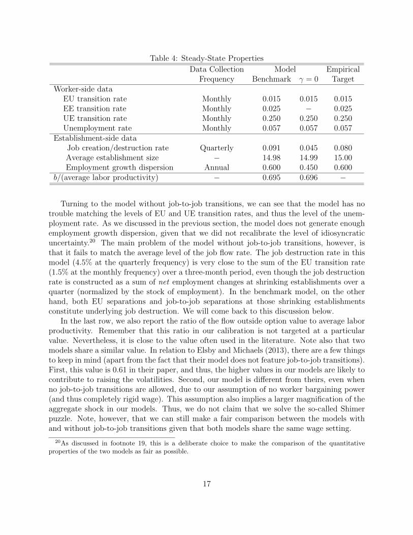
Table 4: Steady-State Properties

Data Collection Model EmpiricalFrequency Benchmark γ = 0 Target

Worker-side dataEU transition rate Monthly 0.015 0.015 0.015EE transition rate Monthly 0.025 − 0.025UE transition rate Monthly 0.250 0.250 0.250Unemployment rate Monthly 0.057 0.057 0.057

Establishment-side dataJob creation/destruction rate Quarterly 0.091 0.045 0.080Average establishment size − 14.98 14.99 15.00Employment growth dispersion Annual 0.600 0.450 0.600

b/(average labor productivity) − 0.695 0.696 −

Turning to the model without job-to-job transitions, we can see that the model has notrouble matching the levels of EU and UE transition rates, and thus the level of the unem-ployment rate. As we discussed in the previous section, the model does not generate enoughemployment growth dispersion, given that we did not recalibrate the level of idiosyncraticuncertainty.20 The main problem of the model without job-to-job transitions, however, isthat it fails to match the average level of the job flow rate. The job destruction rate in thismodel (4.5% at the quarterly frequency) is very close to the sum of the EU transition rate(1.5% at the monthly frequency) over a three-month period, even though the job destructionrate is constructed as a sum of net employment changes at shrinking establishments over aquarter (normalized by the stock of employment). In the benchmark model, on the otherhand, both EU separations and job-to-job separations at those shrinking establishmentsconstitute underlying job destruction. We will come back to this discussion below.

In the last row, we also report the ratio of the flow outside option value to average laborproductivity. Remember that this ratio in our calibration is not targeted at a particularvalue. Nevertheless, it is close to the value often used in the literature. Note also that twomodels share a similar value. In relation to Elsby and Michaels (2013), there are a few thingsto keep in mind (apart from the fact that their model does not feature job-to-job transitions).First, this value is 0.61 in their paper, and thus, the higher values in our models are likely tocontribute to raising the volatilities. Second, our model is different from theirs, even whenno job-to-job transitions are allowed, due to our assumption of no worker bargaining power(and thus completely rigid wage). This assumption also implies a larger magnification of theaggregate shock in our models. Thus, we do not claim that we solve the so-called Shimerpuzzle. Note, however, that we can still make a fair comparison between the models withand without job-to-job transitions given that both models share the same wage setting.

20As discussed in footnote 19, this is a deliberate choice to make the comparison of the quantitativeproperties of the two models as fair as possible.

17

6.2 Hockey Stick Functions

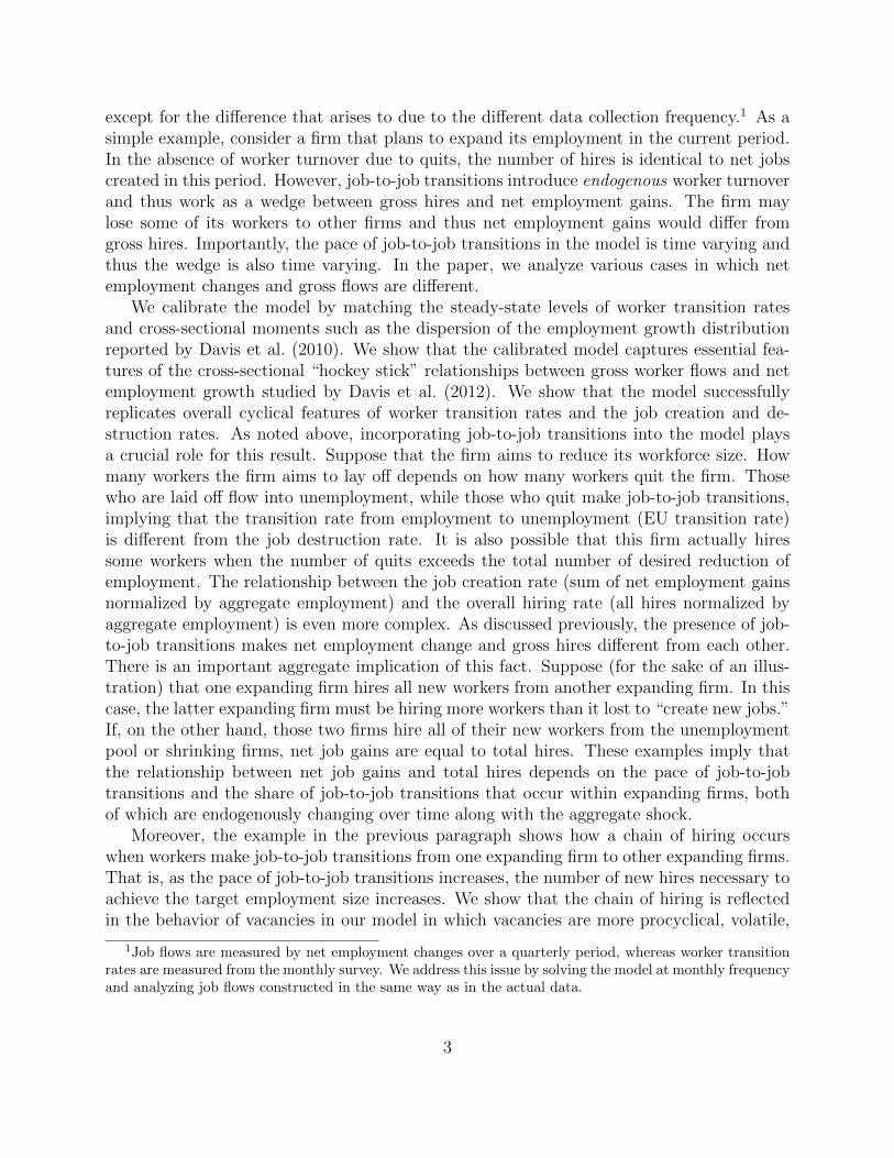
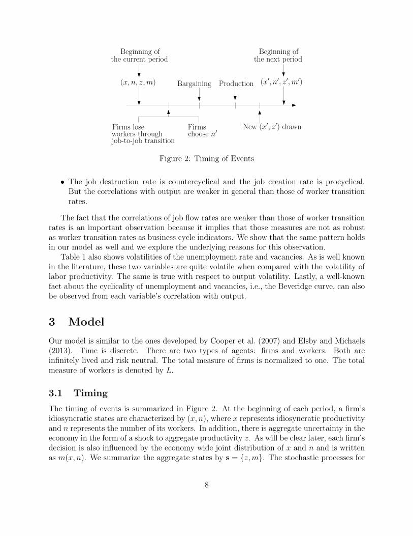
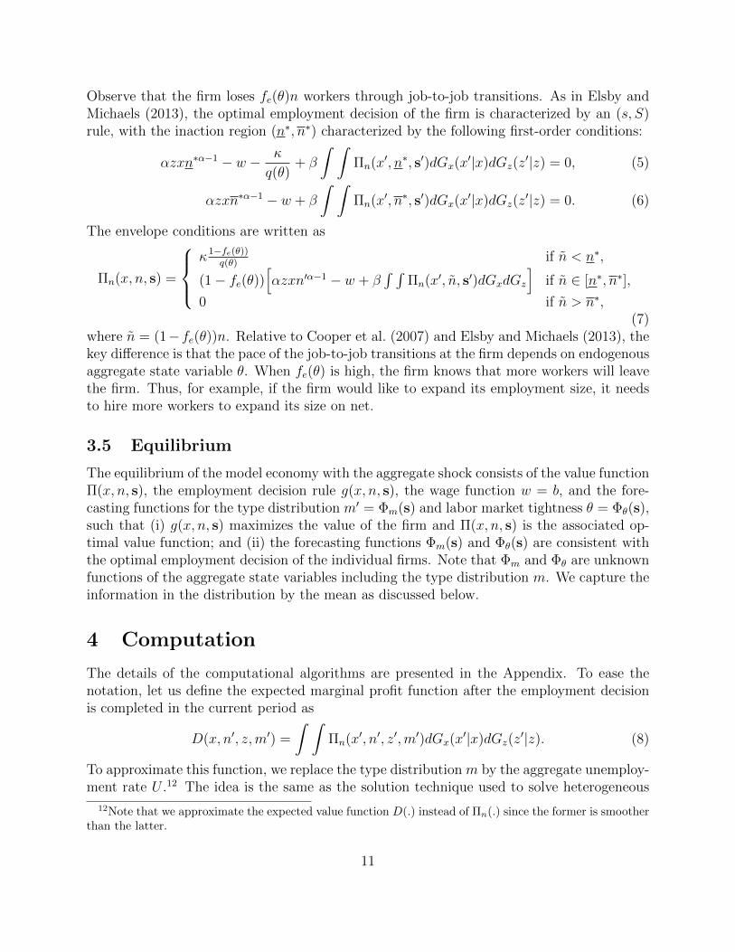
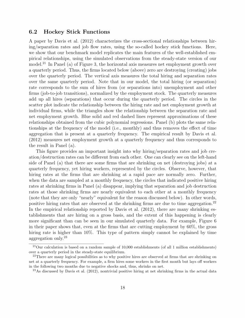
A paper by Davis et al. (2012) characterizes the cross-sectional relationships between hir-ing/separation rates and job flow rates, using the so-called hockey stick functions. Here,we show that our benchmark model replicates the main features of the well-established em-pirical relationships, using the simulated observations from the steady-state version of ourmodel.21 In Panel (a) of Figure 3, the horizontal axis measures net employment growth overa quarterly period. Thus, the firms located below (above) zero are destroying (creating) jobsover the quarterly period. The vertical axis measures the total hiring and separation ratesover the same quarterly period. Note that in our model, the total hiring (or separation)rate corresponds to the sum of hires from (or separations into) unemployment and otherfirms (job-to-job transitions), normalized by the employment stock. The quarterly measuresadd up all hires (separations) that occur during the quarterly period. The circles in thescatter plot indicate the relationship between the hiring rate and net employment growth atindividual firms, while the triangles show the relationship between the separation rate andnet employment growth. Blue solid and red dashed lines represent approximations of theserelationships obtained from the cubic polynomial regressions. Panel (b) plots the same rela-tionships at the frequency of the model (i.e., monthly) and thus removes the effect of timeaggregation that is present at a quarterly frequency. The empirical result by Davis et al.(2012) measures net employment growth at a quarterly frequency and thus corresponds tothe result in Panel (a).

This figure provides an important insight into why hiring/separation rates and job cre-ation/destruction rates can be different from each other. One can clearly see on the left-handside of Panel (a) that there are some firms that are shrinking on net (destroying jobs) at aquarterly frequency, yet hiring workers, represented by the circles. Observe, however, thathiring rates at the firms that are shrinking at a rapid pace are normally zero. Further,when the data are sampled at a monthly frequency, the circles that indicated positive hiringrates at shrinking firms in Panel (a) disappear, implying that separation and job destructionrates at those shrinking firms are nearly equivalent to each other at a monthly frequency(note that they are only “nearly” equivalent for the reason discussed below). In other words,positive hiring rates that are observed at the shrinking firms are due to time aggregation.22

In the empirical relationship reported by Davis et al. (2012), there are many shrinking es-tablishments that are hiring on a gross basis, and the extent of this happening is clearlymore significant than can be seen in our simulated quarterly data. For example, Figure 6in their paper shows that, even at the firms that are cutting employment by 60%, the grosshiring rate is higher than 10%. This type of pattern simply cannot be explained by timeaggregation only.23

21Our calculation is based on a random sample of 10,000 establishments (of all 1 million establishments)over a quarterly period in the steady-state equilibrium.

22There are many logical possibilities as to why positive hires are observed at firms that are shrinking onnet at a quarterly frequency. For example, a firm hires some workers in the first month but lays off workersin the following two months due to negative shocks and, thus, shrinks on net.

23As discussed by Davis et al. (2012), nontrivial positive hiring at net shrinking firms in the actual data

18

(a) Quarterly Data

0.2

.4.6

Per

cent

of E

mpl

oym

ent

−.6 −.4 −.2 0 .2 .4 .6Net Employment Growth

Hiring Rate Separation Rate

Hiring Rate (Cubic Polynomial Approx.) Separation Rate (Cubic Polynomial Approx.)

45 Degree Line 45 Degree Line

(b) Monthly Data

0.1

.2.3

Per

cent

of E

mpl

oym

ent

−.3 −.2 −.1 0 .1 .2 .3Net Employment Growth

Hiring Rate (Monthly) Separation Rate (Monthly)

Hiring Rate (Cubic Polynomial Approx.) Separation Rate (Cubic Polynomial Approx.)

45 Degree Line 45 Degree Line

Figure 3: Hiring/Separation Rate as a Function of Net Employment Growth RateNotes: Based on the 10,000 simulated firm-level observations over quarterly (Panel (a)) and monthly(Panel (b)) periods in the steady-state equilibrium. Blue-solid and red-dashed lines represent predic-tions from the cubic polynomial regressions.

Note that it is incorrect to say, however, that separations and job destruction are thesame to the left of zero in the model (even at a monthly frequency). The equivalence holdsonly at the firms that are making relatively large employment adjustments. One can see inPanel (b) that there is a small region to the immediate left of zero where nonzero hires areobserved. One can also see that, over the same small region, there are more separations thannet employment changes (the red line is located above the 45 degree line). Although thisregion looks small, there are a large number of firms located in this region. For example, 68%of firms are located in the region between 0 and -5% in the steady-state equilibrium. Thisphenomenon corresponds to the scenario in which the firm wants to reduce its employment(thus destroying jobs), but job-to-job transitions are more than enough to achieve the targetemployment level. Thus, these firms end up needing to hire at least some workers. In otherwords, when a firm loses its workers through job-to-job transitions (which generate grossseparations), the firm finds it optimal to partially replace these workers. In this case, hiresand separations coexist within a period, and employment growth is negative. This case isunlikely to occur when a firm receives a large negative shock, in which case the firm is willingto cut its workforce beyond job-to-job transitions.

Next, consider the firms that are located to the right of zero net employment growth (thus

is likely because of some essential positions that the firm needs to refill (after workers leave the firm), eventhough firm size is rapidly shrinking on net. Such a feature is simply not present in our model.

19

creating jobs). One can see in Panel (a) that these firms experience a nontrivial number ofseparations even when they are expanding their employment at a rapid pace. The sameis true even at the monthly frequency displayed in Panel (b), and thus time aggregation isnot the reason for the observed nontrivial separations. In the model, even at the firms thatare growing rapidly, there are always workers leaving for other hiring firms. The pattern ofseparations spreading over the entire range of positive employment growth is consistent withthe empirical fact presented by Davis et al. (2012).24

In summary, the conceptual differences between hiring/separation rates and job cre-ation/destruction rates arise because (i) the firms that are destroying jobs on net may hireworkers and (ii) separations occur at the firms that are creating jobs. The first difference ex-ists only at the firms with small negative employment growth, whereas the second differencearises over entire positive employment growth rates.

Remember that this discussion applies to our benchmark model with job-to-job transi-tions. In the model without job-to-job transitions, neither (i) nor (ii) are true in the modelfrequency. Although time aggregation can generate those features, its effects are very small.Note also that introducing exogenous separations into unemployment easily makes it possibleto produce these two patterns. However, the crucial point is that the pace of separationsat hiring firms varies with business cycles in our model (because of the procyclicality of thejob-to-job transition rate), whereas in the model with exogenous separations, it is invariantwith respect to business cycles.

6.3 Cyclicality of Worker Transition Rates

Table 5 presents the same second-moment statistics discussed earlier in Table 1. As in theprevious analysis, we compare properties of the two models with and without job-to-jobtransitions. Let us first discuss the model without job-to-job transitions (the case withγ = 0). In terms of relative volatilities of UE and EU transition rates, the model does adecent job compared with those of the observed series presented in Table 1, except for severalproblems. The EU transition rate is too volatile relative to the data; and the volatility ofthe EU transition (separation) rate is higher than that of the UE transition (job finding)rate, although the opposite is true in the data.

Overall volatility of this model is large despite the relatively low level of the ratio betweenflow outside option b and average labor productivity (0.70). Here, the fixed wage specificationplays an important role for the large response of both the separation rate and the job findingrate. When a positive aggregate shock hits the economy, hiring firms expand employmentmore under the fixed wage environment than in the flexible wage environment (because wagesdo not rise in this environment). Similarly in a recession, contracting firms respond more inshedding workers because wages do not fall in the fixed wage environment. The correlationpatterns of these two transition rates are largely in line with the data.

24Note, however, that in our model, the separation function is flat on the right-hand side of zero. It ismore plausible that the separation function is downward sloping in that region, because workers are lesslikely to leave more rapidly growing firms. Our model does not generate such a pattern because workersreceive the same wage regardless of the pace of employment growth.

20

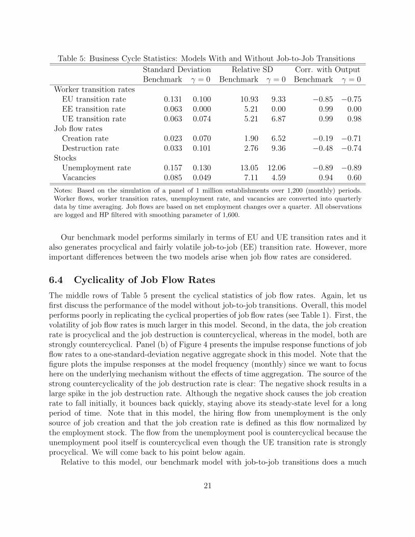
Table 5: Business Cycle Statistics: Models With and Without Job-to-Job Transitions

Standard Deviation Relative SD Corr. with OutputBenchmark γ = 0 Benchmark γ = 0 Benchmark γ = 0

Worker transition ratesEU transition rate 0.131 0.100 10.93 9.33 −0.85 −0.75EE transition rate 0.063 0.000 5.21 0.00 0.99 0.00UE transition rate 0.063 0.074 5.21 6.87 0.99 0.98

Job flow ratesCreation rate 0.023 0.070 1.90 6.52 −0.19 −0.71Destruction rate 0.033 0.101 2.76 9.36 −0.48 −0.74

StocksUnemployment rate 0.157 0.130 13.05 12.06 −0.89 −0.89Vacancies 0.085 0.049 7.11 4.59 0.94 0.60

Notes: Based on the simulation of a panel of 1 million establishments over 1,200 (monthly) periods.Worker flows, worker transition rates, unemployment rate, and vacancies are converted into quarterlydata by time averaging. Job flows are based on net employment changes over a quarter. All observationsare logged and HP filtered with smoothing parameter of 1,600.

Our benchmark model performs similarly in terms of EU and UE transition rates and italso generates procyclical and fairly volatile job-to-job (EE) transition rate. However, moreimportant differences between the two models arise when job flow rates are considered.

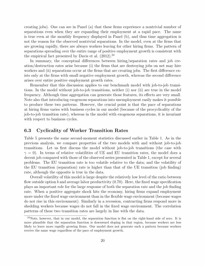
6.4 Cyclicality of Job Flow Rates

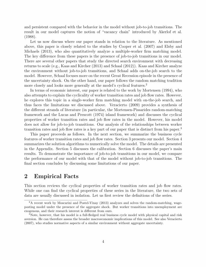
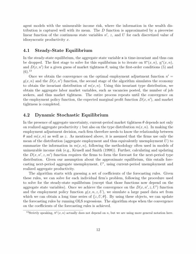
The middle rows of Table 5 present the cyclical statistics of job flow rates. Again, let usfirst discuss the performance of the model without job-to-job transitions. Overall, this modelperforms poorly in replicating the cyclical properties of job flow rates (see Table 1). First, thevolatility of job flow rates is much larger in this model. Second, in the data, the job creationrate is procyclical and the job destruction is countercyclical, whereas in the model, both arestrongly countercyclical. Panel (b) of Figure 4 presents the impulse response functions of jobflow rates to a one-standard-deviation negative aggregate shock in this model. Note that thefigure plots the impulse responses at the model frequency (monthly) since we want to focushere on the underlying mechanism without the effects of time aggregation. The source of thestrong countercyclicality of the job destruction rate is clear: The negative shock results in alarge spike in the job destruction rate. Although the negative shock causes the job creationrate to fall initially, it bounces back quickly, staying above its steady-state level for a longperiod of time. Note that in this model, the hiring flow from unemployment is the onlysource of job creation and that the job creation rate is defined as this flow normalized bythe employment stock. The flow from the unemployment pool is countercyclical because theunemployment pool itself is countercyclical even though the UE transition rate is stronglyprocyclical. We will come back to his point below again.

Relative to this model, our benchmark model with job-to-job transitions does a much

21

(a) Benchmark Model

-0.04

-0.02

0

0.02

0.04

0 3 6 9 12 15 18 21 24

Month

Job creation rate

Job destruction rate

(b) Model with No Job-to-Job Transitions

-0.04

-0.02

0

0.02

0.04

0.06

0.08

0.1

0 3 6 9 12 15 18 21 24

Month

Job creation rate

Job destruction rate

Figure 4: Impulse Response Functions of Job Flow RatesNotes: Plotted are responses to a one-standard-deviation negative aggregate shock expressed as logdeviations from the steady-state levels.

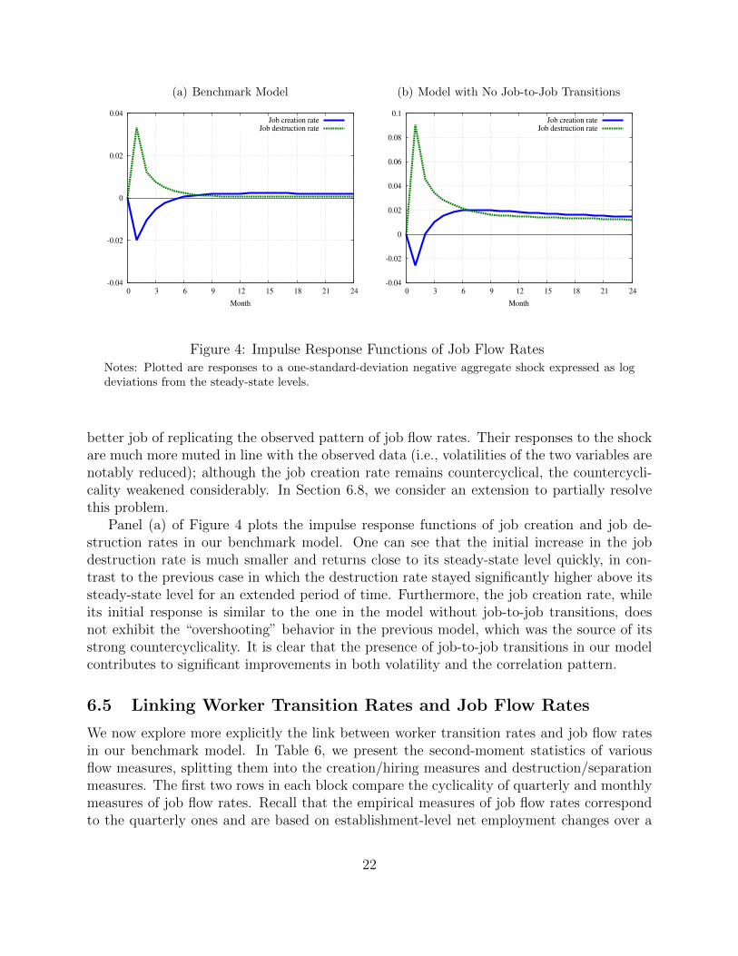
better job of replicating the observed pattern of job flow rates. Their responses to the shockare much more muted in line with the observed data (i.e., volatilities of the two variables arenotably reduced); although the job creation rate remains countercyclical, the countercycli-cality weakened considerably. In Section 6.8, we consider an extension to partially resolvethis problem.

Panel (a) of Figure 4 plots the impulse response functions of job creation and job de-struction rates in our benchmark model. One can see that the initial increase in the jobdestruction rate is much smaller and returns close to its steady-state level quickly, in con-trast to the previous case in which the destruction rate stayed significantly higher above itssteady-state level for an extended period of time. Furthermore, the job creation rate, whileits initial response is similar to the one in the model without job-to-job transitions, doesnot exhibit the “overshooting” behavior in the previous model, which was the source of itsstrong countercyclicality. It is clear that the presence of job-to-job transitions in our modelcontributes to significant improvements in both volatility and the correlation pattern.

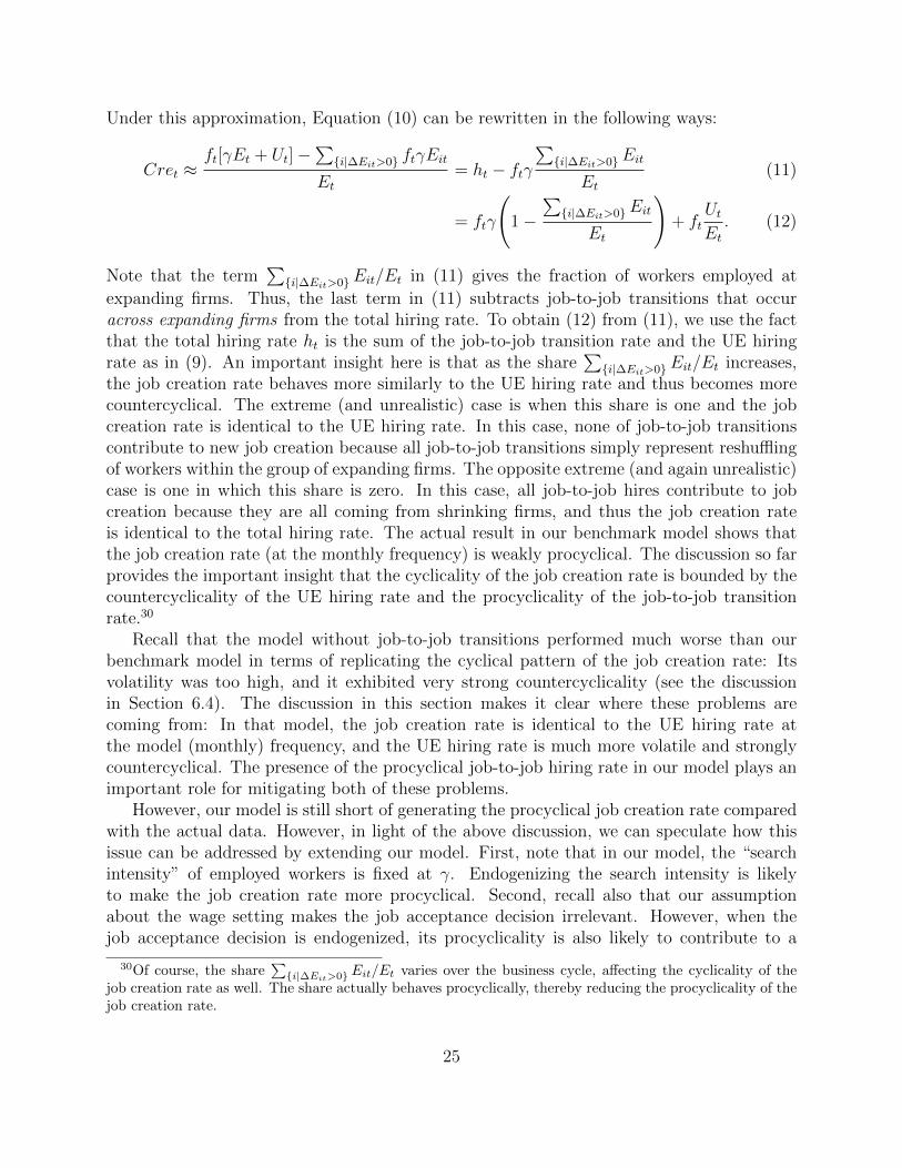
6.5 Linking Worker Transition Rates and Job Flow Rates

We now explore more explicitly the link between worker transition rates and job flow ratesin our benchmark model. In Table 6, we present the second-moment statistics of variousflow measures, splitting them into the creation/hiring measures and destruction/separationmeasures. The first two rows in each block compare the cyclicality of quarterly and monthlymeasures of job flow rates. Recall that the empirical measures of job flow rates correspondto the quarterly ones and are based on establishment-level net employment changes over a

22

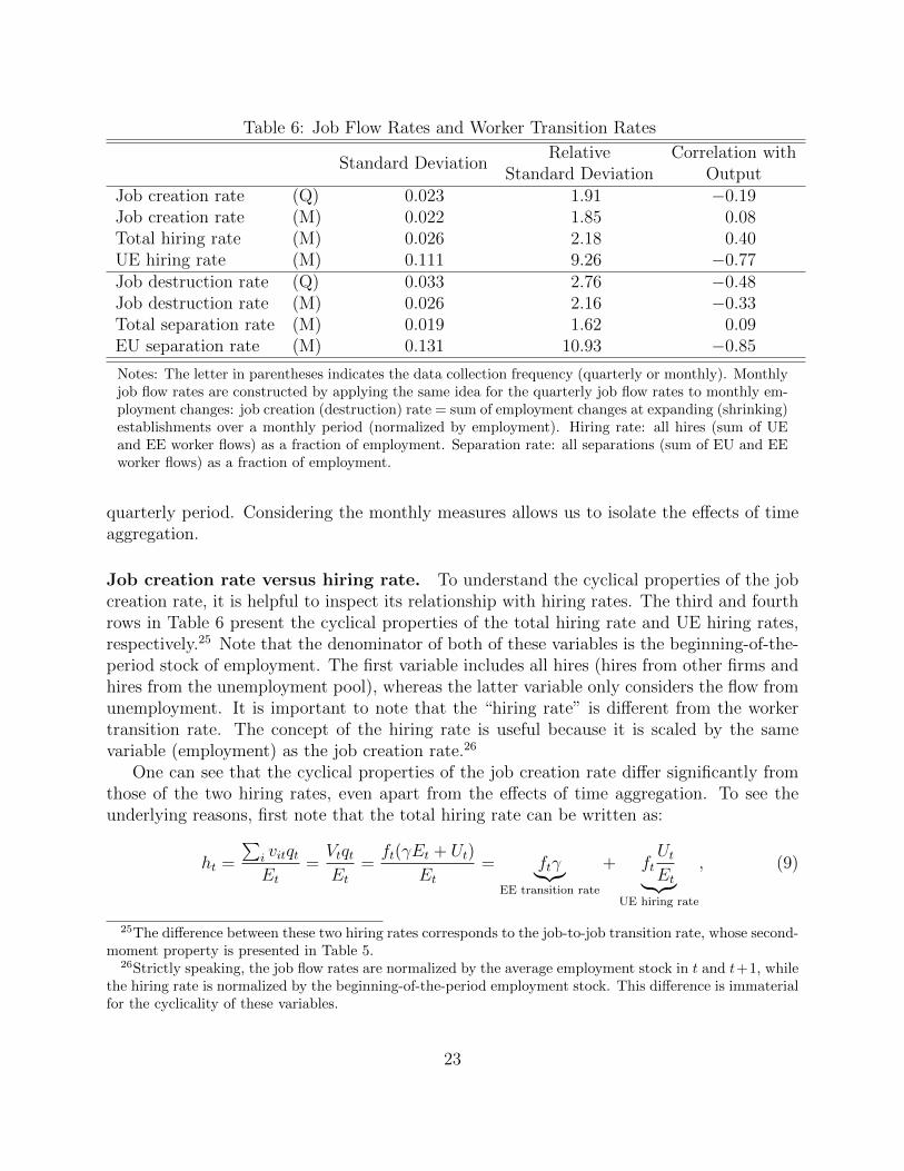
Table 6: Job Flow Rates and Worker Transition Rates

Standard DeviationRelative Correlation with

Standard Deviation OutputJob creation rate (Q) 0.023 1.91 −0.19Job creation rate (M) 0.022 1.85 0.08Total hiring rate (M) 0.026 2.18 0.40UE hiring rate (M) 0.111 9.26 −0.77Job destruction rate (Q) 0.033 2.76 −0.48Job destruction rate (M) 0.026 2.16 −0.33Total separation rate (M) 0.019 1.62 0.09EU separation rate (M) 0.131 10.93 −0.85

Notes: The letter in parentheses indicates the data collection frequency (quarterly or monthly). Monthlyjob flow rates are constructed by applying the same idea for the quarterly job flow rates to monthly em-ployment changes: job creation (destruction) rate = sum of employment changes at expanding (shrinking)establishments over a monthly period (normalized by employment). Hiring rate: all hires (sum of UEand EE worker flows) as a fraction of employment. Separation rate: all separations (sum of EU and EEworker flows) as a fraction of employment.

quarterly period. Considering the monthly measures allows us to isolate the effects of timeaggregation.

Job creation rate versus hiring rate. To understand the cyclical properties of the jobcreation rate, it is helpful to inspect its relationship with hiring rates. The third and fourthrows in Table 6 present the cyclical properties of the total hiring rate and UE hiring rates,respectively.25 Note that the denominator of both of these variables is the beginning-of-the-period stock of employment. The first variable includes all hires (hires from other firms andhires from the unemployment pool), whereas the latter variable only considers the flow fromunemployment. It is important to note that the “hiring rate” is different from the workertransition rate. The concept of the hiring rate is useful because it is scaled by the samevariable (employment) as the job creation rate.26

One can see that the cyclical properties of the job creation rate differ significantly fromthose of the two hiring rates, even apart from the effects of time aggregation. To see theunderlying reasons, first note that the total hiring rate can be written as:

ht =

∑i vitqtEt

=VtqtEt

=ft(γEt + Ut)

Et= ftγ︸︷︷︸

EE transition rate

+ ftUtEt︸︷︷︸

UE hiring rate

, (9)

25The difference between these two hiring rates corresponds to the job-to-job transition rate, whose second-moment property is presented in Table 5.

26Strictly speaking, the job flow rates are normalized by the average employment stock in t and t+1, whilethe hiring rate is normalized by the beginning-of-the-period employment stock. This difference is immaterialfor the cyclicality of these variables.

23

where Vit is the number of vacancies posted at establishment i in t; Vt is the aggregatenumber of vacancies in t; Et is the employment stock at the beginning of t; qt and ft arethe job filling rate and the job finding rate, respectively, in t and should be understood as afunction of market tightness θt. The two terms after the last equality are, respectively, thejob-to-job (EE) transition rate and the hiring rate from the unemployment rate. Clearly, thejob-to-job (EE) transition rate is procyclical as a direct effect of ft. On the other hand, thehiring rate from unemployment is strongly countercyclical, as indicated by the fourth rowof Table 6. This is because the strong countercyclicality of Ut/Et dominates the procyclicaleffect of ft. Note also that even though the volatility of the UE hiring rate is large, thetotal hiring rate is much less volatile. The reason is the negative correlation between theprocyclical job-to-job transition rate and the countercyclical UE hiring rate. The total hiringrate turns to be procyclical because the volume of job-to-job hires is larger than that of UEhires and thus the procyclicality of the former variable is dominant.27

Table 6 also indicates interestingly that the total hiring rate is quite a different objectfrom the job creation rate. In particular, although the procyclicality of the total hiringrate is relatively strong, this procyclicality nearly disappears when the job creation rate isconsidered. To see the source of this difference, let us write the job creation rate (at monthlyfrequency) Cret as follows:28

Cret =

∑{i|∆Eit>0}(qtvit − ftγEit)

Et. (10)

This definition aggregates net employment changes at expanding firms. The first term onthe right-hand side aggregates vacancies posted at those expanding firms only. In the model,there exist vacancies posted at firms that are shrinking on net. As discussed before, thesevacancies are posted in order to replace some of the workers that are lost through job-to-job transitions (and thus these firms are shrinking on net). However, the vast majority ofvacancies are posted at expanding firms. In the steady state, more than 98% of vacanciescome from expanding firms.29 This observation allows us to adopt the following usefulapproximation: ∑

{i|∆Eit>0}

vit ≈ Vt.

27Note that in our calibration, γ = 0.1 and U/E = 0.06 in the steady state. Thus, the cyclicality of thejob-to-job transition rate carries more weight.

28Note that the following definition uses, for simplicity, the beginning-of-the-period stock of employmentas a normalizing factor (instead of the average of the two periods as suggested by the original definition).However, this simplification bears no material implications for our quantitative analysis.

29This share obviously depends on calibration. However, given that the level of the job-to-job transitionrate in the model is calibrated to the observed data, there is little room for this share to be different.

24

Under this approximation, Equation (10) can be rewritten in the following ways:

Cret ≈ft[γEt + Ut]−

∑{i|∆Eit>0} ftγEit

Et= ht − ftγ

∑{i|∆Eit>0}Eit

Et(11)

= ftγ

(1−

∑{i|∆Eit>0}Eit

Et

)+ ft

UtEt. (12)

Note that the term∑{i|∆Eit>0}Eit/Et in (11) gives the fraction of workers employed at

expanding firms. Thus, the last term in (11) subtracts job-to-job transitions that occuracross expanding firms from the total hiring rate. To obtain (12) from (11), we use the factthat the total hiring rate ht is the sum of the job-to-job transition rate and the UE hiringrate as in (9). An important insight here is that as the share

∑{i|∆Eit>0}Eit/Et increases,

the job creation rate behaves more similarly to the UE hiring rate and thus becomes morecountercyclical. The extreme (and unrealistic) case is when this share is one and the jobcreation rate is identical to the UE hiring rate. In this case, none of job-to-job transitionscontribute to new job creation because all job-to-job transitions simply represent reshufflingof workers within the group of expanding firms. The opposite extreme (and again unrealistic)case is one in which this share is zero. In this case, all job-to-job hires contribute to jobcreation because they are all coming from shrinking firms, and thus the job creation rateis identical to the total hiring rate. The actual result in our benchmark model shows thatthe job creation rate (at the monthly frequency) is weakly procyclical. The discussion so farprovides the important insight that the cyclicality of the job creation rate is bounded by thecountercyclicality of the UE hiring rate and the procyclicality of the job-to-job transitionrate.30

Recall that the model without job-to-job transitions performed much worse than ourbenchmark model in terms of replicating the cyclical pattern of the job creation rate: Itsvolatility was too high, and it exhibited very strong countercyclicality (see the discussionin Section 6.4). The discussion in this section makes it clear where these problems arecoming from: In that model, the job creation rate is identical to the UE hiring rate atthe model (monthly) frequency, and the UE hiring rate is much more volatile and stronglycountercyclical. The presence of the procyclical job-to-job hiring rate in our model plays animportant role for mitigating both of these problems.

However, our model is still short of generating the procyclical job creation rate comparedwith the actual data. However, in light of the above discussion, we can speculate how thisissue can be addressed by extending our model. First, note that in our model, the “searchintensity” of employed workers is fixed at γ. Endogenizing the search intensity is likelyto make the job creation rate more procyclical. Second, recall also that our assumptionabout the wage setting makes the job acceptance decision irrelevant. However, when thejob acceptance decision is endogenized, its procyclicality is also likely to contribute to a

30Of course, the share∑{i|∆Eit>0}Eit/Et varies over the business cycle, affecting the cyclicality of the

job creation rate as well. The share actually behaves procyclically, thereby reducing the procyclicality of thejob creation rate.

25

higher procyclicality of the total hiring rate and thus the job creation rate. Lastly, the moreprocyclical job finding rate ft itself will be an effective remedy for this problem as well.

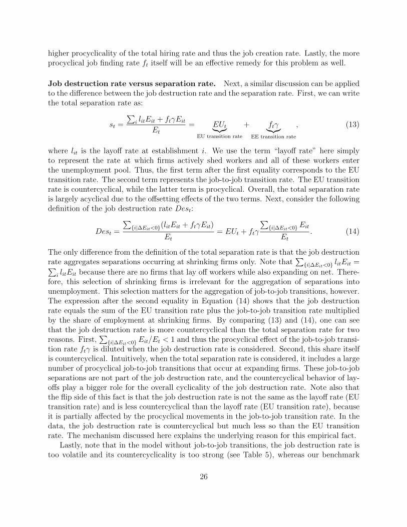
Job destruction rate versus separation rate. Next, a similar discussion can be appliedto the difference between the job destruction rate and the separation rate. First, we can writethe total separation rate as:

st =

∑i litEit + ftγEit

Et= EUt︸︷︷︸

EU transition rate

+ ftγ︸︷︷︸EE transition rate

, (13)

where lit is the layoff rate at establishment i. We use the term “layoff rate” here simplyto represent the rate at which firms actively shed workers and all of these workers enterthe unemployment pool. Thus, the first term after the first equality corresponds to the EUtransition rate. The second term represents the job-to-job transition rate. The EU transitionrate is countercyclical, while the latter term is procyclical. Overall, the total separation rateis largely acyclical due to the offsetting effects of the two terms. Next, consider the followingdefinition of the job destruction rate Dest:

Dest =

∑{i|∆Eit<0}(litEit + ftγEit)

Et= EUt + ftγ

∑{i|∆Eit<0}Eit

Et. (14)

The only difference from the definition of the total separation rate is that the job destructionrate aggregates separations occurring at shrinking firms only. Note that

∑{i|∆Eit<0} litEit =∑

i litEit because there are no firms that lay off workers while also expanding on net. There-fore, this selection of shrinking firms is irrelevant for the aggregation of separations intounemployment. This selection matters for the aggregation of job-to-job transitions, however.The expression after the second equality in Equation (14) shows that the job destructionrate equals the sum of the EU transition rate plus the job-to-job transition rate multipliedby the share of employment at shrinking firms. By comparing (13) and (14), one can seethat the job destruction rate is more countercyclical than the total separation rate for tworeasons. First,

∑{i|∆Eit<0}Eit/Et < 1 and thus the procyclical effect of the job-to-job transi-

tion rate ftγ is diluted when the job destruction rate is considered. Second, this share itselfis countercyclical. Intuitively, when the total separation rate is considered, it includes a largenumber of procyclical job-to-job transitions that occur at expanding firms. These job-to-jobseparations are not part of the job destruction rate, and the countercyclical behavior of lay-offs play a bigger role for the overall cyclicality of the job destruction rate. Note also thatthe flip side of this fact is that the job destruction rate is not the same as the layoff rate (EUtransition rate) and is less countercyclical than the layoff rate (EU transition rate), becauseit is partially affected by the procyclical movements in the job-to-job transition rate. In thedata, the job destruction rate is countercyclical but much less so than the EU transitionrate. The mechanism discussed here explains the underlying reason for this empirical fact.

Lastly, note that in the model without job-to-job transitions, the job destruction rate istoo volatile and its countercyclicality is too strong (see Table 5), whereas our benchmark

26

(a) Unemployment and Vacancies

-0.06

-0.03

0

0.03

0.06

0.09

0.12

0 3 6 9 12 15 18 21 24

Month

Unemployment (benchmark)Vacancies (benchmark)

Unemployment (no job-to-job transitions)Vacancies (no job-to-job transitions)

(b) Job-to-Job Transition Rate

-0.04

-0.02

0

0.02

0 3 6 9 12 15 18 21 24

Month

Job-to-job transition rate (benchmark)

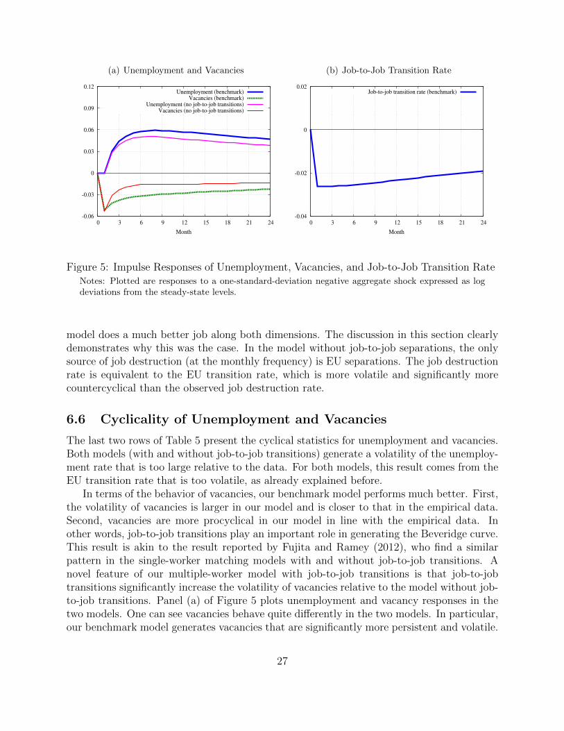
Figure 5: Impulse Responses of Unemployment, Vacancies, and Job-to-Job Transition RateNotes: Plotted are responses to a one-standard-deviation negative aggregate shock expressed as logdeviations from the steady-state levels.

model does a much better job along both dimensions. The discussion in this section clearlydemonstrates why this was the case. In the model without job-to-job separations, the onlysource of job destruction (at the monthly frequency) is EU separations. The job destructionrate is equivalent to the EU transition rate, which is more volatile and significantly morecountercyclical than the observed job destruction rate.

6.6 Cyclicality of Unemployment and Vacancies

The last two rows of Table 5 present the cyclical statistics for unemployment and vacancies.Both models (with and without job-to-job transitions) generate a volatility of the unemploy-ment rate that is too large relative to the data. For both models, this result comes from theEU transition rate that is too volatile, as already explained before.

In terms of the behavior of vacancies, our benchmark model performs much better. First,the volatility of vacancies is larger in our model and is closer to that in the empirical data.Second, vacancies are more procyclical in our model in line with the empirical data. Inother words, job-to-job transitions play an important role in generating the Beveridge curve.This result is akin to the result reported by Fujita and Ramey (2012), who find a similarpattern in the single-worker matching models with and without job-to-job transitions. Anovel feature of our multiple-worker model with job-to-job transitions is that job-to-jobtransitions significantly increase the volatility of vacancies relative to the model without job-to-job transitions. Panel (a) of Figure 5 plots unemployment and vacancy responses in thetwo models. One can see vacancies behave quite differently in the two models. In particular,our benchmark model generates vacancies that are significantly more persistent and volatile.

27

0.1

.2.3

Shar

e of

Em

ploy

men

t

-.3 -.2 -.1 0 .1 .2 .3(Monthly) Net Employment Growth

Hiring Rate (Boom) Separation Rate (Boom)

Hiring Rate (Recession) Separation Rate (Recession)

45 Degree 45 Degree

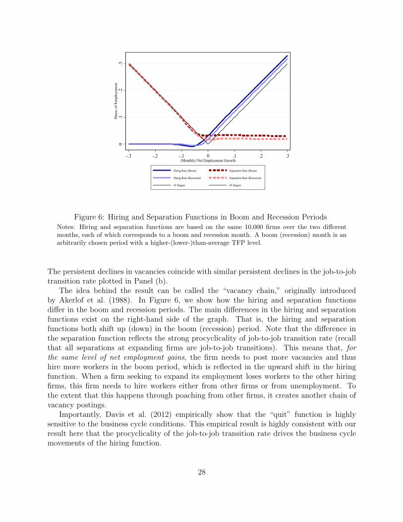
Figure 6: Hiring and Separation Functions in Boom and Recession PeriodsNotes: Hiring and separation functions are based on the same 10,000 firms over the two differentmonths, each of which corresponds to a boom and recession month. A boom (recession) month is anarbitrarily chosen period with a higher-(lower-)than-average TFP level.

The persistent declines in vacancies coincide with similar persistent declines in the job-to-jobtransition rate plotted in Panel (b).

The idea behind the result can be called the “vacancy chain,” originally introducedby Akerlof et al. (1988). In Figure 6, we show how the hiring and separation functionsdiffer in the boom and recession periods. The main differences in the hiring and separationfunctions exist on the right-hand side of the graph. That is, the hiring and separationfunctions both shift up (down) in the boom (recession) period. Note that the difference inthe separation function reflects the strong procyclicality of job-to-job transition rate (recallthat all separations at expanding firms are job-to-job transitions). This means that, forthe same level of net employment gains, the firm needs to post more vacancies and thushire more workers in the boom period, which is reflected in the upward shift in the hiringfunction. When a firm seeking to expand its employment loses workers to the other hiringfirms, this firm needs to hire workers either from other firms or from unemployment. Tothe extent that this happens through poaching from other firms, it creates another chain ofvacancy postings.

Importantly, Davis et al. (2012) empirically show that the “quit” function is highlysensitive to the business cycle conditions. This empirical result is highly consistent with ourresult here that the procyclicality of the job-to-job transition rate drives the business cyclemovements of the hiring function.

28

6.7 Robustness

While our model is fairly tightly calibrated, it is worth checking whether the quantitativeresults are robust with respect to the variations of some of the exogenously chosen parame-ters. In particular, we considered the cases in which we set the curvature parameter of theproduction function α at 0.67, the persistence parameter of the idiosyncratic shock ρz at 0.9and 0.99, and the elasticity parameter of the matching function at 0.6 instead of the valuesin the benchmark calibration. For each alternative value, we recalibrate the model followingexactly the same procedure as in the benchmark calibration. We find that all the resultsunder the benchmark calibration go through in those three cases. The results are availableupon request.

6.8 Introducing a Firing Cost

In this section, we discuss the results from a simple extension of the model, namely, intro-duction of the firing cost. We adopt the simplest possible specification in which the costper layoff is constant at τ .31 Recall that, in our benchmark model, the job creation rate isweakly countercyclical, while in the data it is procyclical. Our earlier discussion in Section6.5 suggests that one of the factors affecting the cyclicality of the job creation rate is therelative strength of the countercyclicality of the EU transition rate and the procyclicalityof the job-to-job transition rate. Thus, introducing the firing cost can potentially shift thisbalance in the procyclical direction. In calibrating the model with the firing cost, we keepall the existing parameters at the same values as before and set the value of τ at 25% ofmonthly wage, which is fairly low and thus is in line with the fact that the firing cost inthe U.S. is, on average, very small.32 We also consider the case in which the firing cost isintroduced into the model without job-to-job transitions. Again, we simply set the value ofτ at 25% of the monthly wage without changing other parameter values.

Table 7 compares relative standard deviations and correlations with output in the fourcases (models with and without job-to-job transitions and the firing cost). First, observethat in the model without job-to-job transitions, the introduction of the small firing costslightly reduces the volatility of the EU transition rate and the unemployment rate (thevolatility of the UE transition rate, on the other hand, increases slightly). Job creationand destruction rates become less volatile but remain too volatile relative to the empiricalmoments. Moreover, both of them remain strongly countercyclical. Overall, the cyclicalproperties of this model are largely insensitive to the introduction of the small firing cost.

More interesting interactions exist in the model with job-to-job transitions. In particular,the relative standard deviations of all transition rates increase with the introduction of the

31The optimality conditions presented in Section 3.4 needs to be modified in a straightforward mannerwith the introduction τ .

32We do not recalibrate the model for this exercise since recalibrating requires us to change the valuesof other parameters, making it difficult to isolate the effects of the introduction of τ . Because we do notrecalibrate the model, introducing the firing cost has an effect of lowering the steady-state worker transitionrates. However, its quantitative impacts are fairly small. The steady-state EU transition and UE transitionrates fall to 1.3% and 23% from 1.5% and 25%, respectively.

29

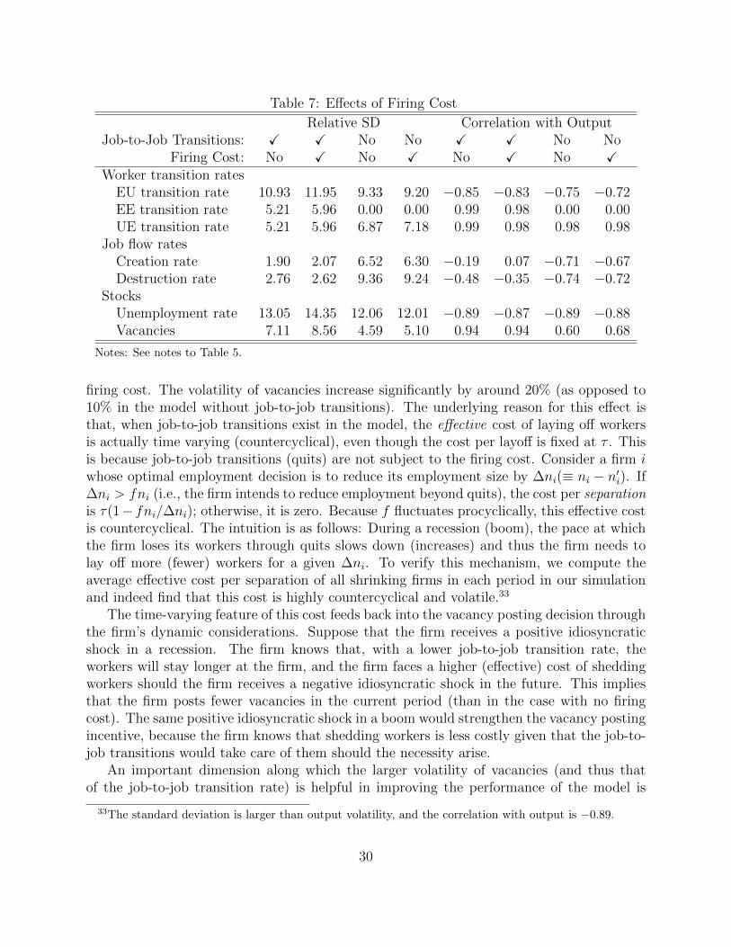
Table 7: Effects of Firing Cost

Relative SD Correlation with OutputJob-to-Job Transitions: X X No No X X No No

Firing Cost: No X No X No X No XWorker transition rates

EU transition rate 10.93 11.95 9.33 9.20 −0.85 −0.83 −0.75 −0.72EE transition rate 5.21 5.96 0.00 0.00 0.99 0.98 0.00 0.00UE transition rate 5.21 5.96 6.87 7.18 0.99 0.98 0.98 0.98

Job flow ratesCreation rate 1.90 2.07 6.52 6.30 −0.19 0.07 −0.71 −0.67Destruction rate 2.76 2.62 9.36 9.24 −0.48 −0.35 −0.74 −0.72

StocksUnemployment rate 13.05 14.35 12.06 12.01 −0.89 −0.87 −0.89 −0.88Vacancies 7.11 8.56 4.59 5.10 0.94 0.94 0.60 0.68

Notes: See notes to Table 5.

firing cost. The volatility of vacancies increase significantly by around 20% (as opposed to10% in the model without job-to-job transitions). The underlying reason for this effect isthat, when job-to-job transitions exist in the model, the effective cost of laying off workersis actually time varying (countercyclical), even though the cost per layoff is fixed at τ . Thisis because job-to-job transitions (quits) are not subject to the firing cost. Consider a firm iwhose optimal employment decision is to reduce its employment size by ∆ni(≡ ni − n′i). If∆ni > fni (i.e., the firm intends to reduce employment beyond quits), the cost per separationis τ(1− fni/∆ni); otherwise, it is zero. Because f fluctuates procyclically, this effective costis countercyclical. The intuition is as follows: During a recession (boom), the pace at whichthe firm loses its workers through quits slows down (increases) and thus the firm needs tolay off more (fewer) workers for a given ∆ni. To verify this mechanism, we compute theaverage effective cost per separation of all shrinking firms in each period in our simulationand indeed find that this cost is highly countercyclical and volatile.33

The time-varying feature of this cost feeds back into the vacancy posting decision throughthe firm’s dynamic considerations. Suppose that the firm receives a positive idiosyncraticshock in a recession. The firm knows that, with a lower job-to-job transition rate, theworkers will stay longer at the firm, and the firm faces a higher (effective) cost of sheddingworkers should the firm receives a negative idiosyncratic shock in the future. This impliesthat the firm posts fewer vacancies in the current period (than in the case with no firingcost). The same positive idiosyncratic shock in a boom would strengthen the vacancy postingincentive, because the firm knows that shedding workers is less costly given that the job-to-job transitions would take care of them should the necessity arise.

An important dimension along which the larger volatility of vacancies (and thus thatof the job-to-job transition rate) is helpful in improving the performance of the model is

33The standard deviation is larger than output volatility, and the correlation with output is −0.89.

30

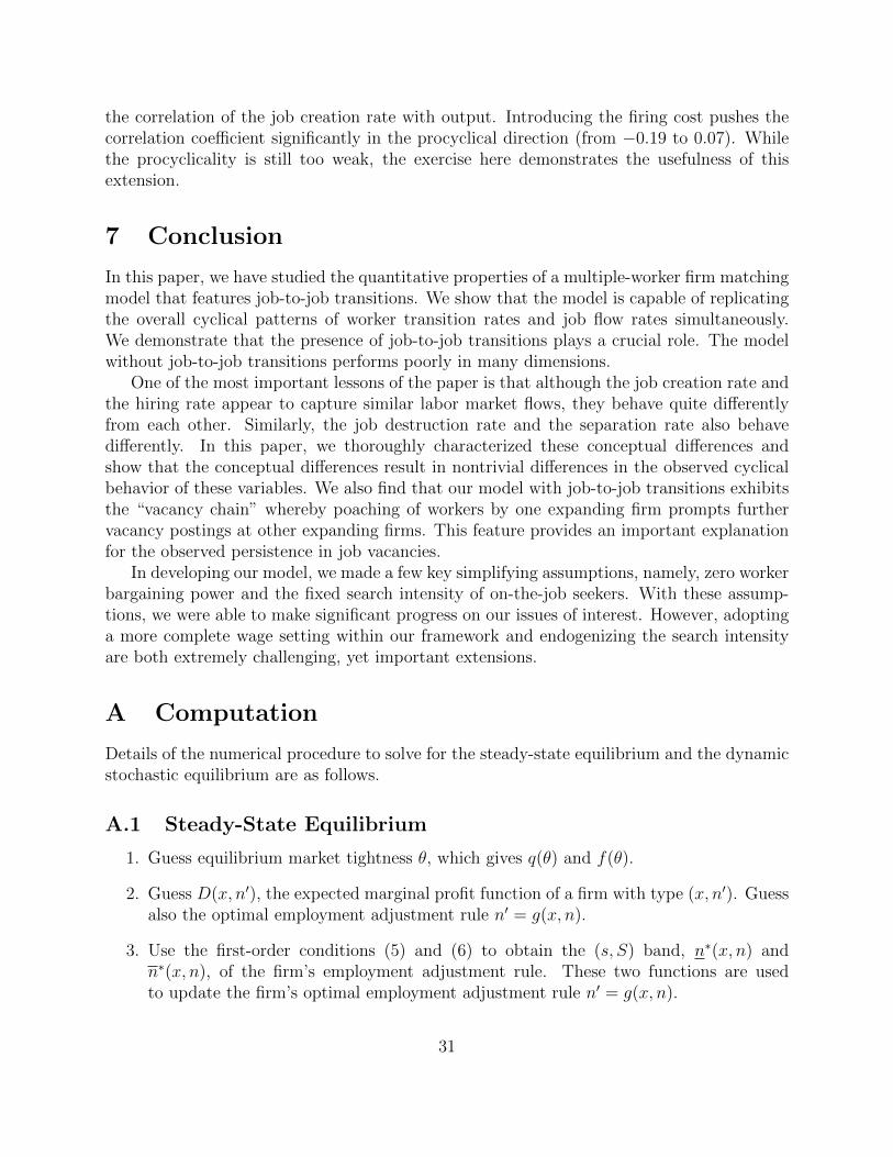
the correlation of the job creation rate with output. Introducing the firing cost pushes thecorrelation coefficient significantly in the procyclical direction (from −0.19 to 0.07). Whilethe procyclicality is still too weak, the exercise here demonstrates the usefulness of thisextension.

7 Conclusion

In this paper, we have studied the quantitative properties of a multiple-worker firm matchingmodel that features job-to-job transitions. We show that the model is capable of replicatingthe overall cyclical patterns of worker transition rates and job flow rates simultaneously.We demonstrate that the presence of job-to-job transitions plays a crucial role. The modelwithout job-to-job transitions performs poorly in many dimensions.

One of the most important lessons of the paper is that although the job creation rate andthe hiring rate appear to capture similar labor market flows, they behave quite differentlyfrom each other. Similarly, the job destruction rate and the separation rate also behavedifferently. In this paper, we thoroughly characterized these conceptual differences andshow that the conceptual differences result in nontrivial differences in the observed cyclicalbehavior of these variables. We also find that our model with job-to-job transitions exhibitsthe “vacancy chain” whereby poaching of workers by one expanding firm prompts furthervacancy postings at other expanding firms. This feature provides an important explanationfor the observed persistence in job vacancies.

In developing our model, we made a few key simplifying assumptions, namely, zero workerbargaining power and the fixed search intensity of on-the-job seekers. With these assump-tions, we were able to make significant progress on our issues of interest. However, adoptinga more complete wage setting within our framework and endogenizing the search intensityare both extremely challenging, yet important extensions.

A Computation

Details of the numerical procedure to solve for the steady-state equilibrium and the dynamicstochastic equilibrium are as follows.

A.1 Steady-State Equilibrium

1. Guess equilibrium market tightness θ, which gives q(θ) and f(θ).

2. Guess D(x, n′), the expected marginal profit function of a firm with type (x, n′). Guessalso the optimal employment adjustment rule n′ = g(x, n).

3. Use the first-order conditions (5) and (6) to obtain the (s, S) band, n∗(x, n) andn∗(x, n), of the firm’s employment adjustment rule. These two functions are usedto update the firm’s optimal employment adjustment rule n′ = g(x, n).

31

4. Using the updated optimal employment adjustment rule n′ = g(x, n), (7), and (8),update the firm’s marginal profit function D(x, n′).

5. Check convergence of D(x, n′) and n′ = g(x, n), based on the distance between the oldand updated functions. If convergence is obtained, go to the next step. Otherwise,update D(x, n′) and n′ = g(x, n) and go back to Step 3.

6. Using the optimal employment adjustment rule n′ = g(x, n) and the stochastic processfor x, simulate the economy until the invariant type distribution m(x, n) is obtained.

7. Compute the total labor force (population) consistent with the stationary distributionm and the unemployment rate U as

L =

∫g(x, n)dm

1− U .

Note that U is fixed at a targeted level. In other words, we don’t need to find anequilibrium U because we impose it to be exactly our target value. The efficiency-weighted number of searchers S, the total number of vacancies (normalized by thelabor force) V , and the labor market tightness θ are calculated by

S = γ(1− U) + U, (15)

V =1

L

∫max[g(x, n)− (1− γf(θ))n, 0]

q(θ)dm, (16)

θ =V

S. (17)

8. Check convergence of θ. If the distance between the guess and the updated numbersis smaller than the predetermined value, then stop. Otherwise, update θ and go backto Step 2.

A.2 Dynamic Stochastic Equilibrium

1. Set up the equilibrium forecasting functions. Note that the type distribution m isreplaced by U . {U ′, θ} is the list of variables to be forecast through the followingforecasting rules:

logU ′ = φ10 + φ1

1 log z + φ12 logU (18)

log θ = φ20 + φ2

1 log z + φ22 logU (19)

Let Φ be the vector of the parameters {φi0, φi1, φi2}i=1,2.

2. With a guess for Φ, and current z and U , we can predict q(θ), f(θ), and U ′.

3. Guess the expected marginal profit of the firm with a type (x, n′) under the aggregatestate (z, U ′), D(x, n′, z, U ′).

32

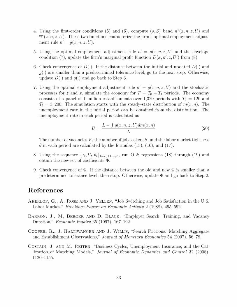
4. Using the first-order conditions (5) and (6), compute (s, S) band n∗(x, n, z, U) andn∗(x, n, z, U). These two functions characterize the firm’s optimal employment adjust-ment rule n′ = g(x, n, z, U).

5. Using the optimal employment adjustment rule n′ = g(x, n, z, U) and the envelopecondition (7), update the firm’s marginal profit function D(x, n′, z, U ′) from (8).

6. Check convergence of D(.). If the distance between the initial and updated D(.) andg(.) are smaller than a predetermined tolerance level, go to the next step. Otherwise,update D(.) and g(.) and go back to Step 3.

7. Using the optimal employment adjustment rule n′ = g(x, n, z, U) and the stochasticprocesses for z and x, simulate the economy for T = T0 + T1 periods. The economyconsists of a panel of 1 million establishments over 1,320 periods with T0 = 120 andT1 = 3, 200. The simulation starts with the steady-state distribution of m(x, n). Theunemployment rate in the initial period can be obtained from the distribution. Theunemployment rate in each period is calculated as

U =L−

∫g(x, n, z, U)dm(x, n)

L. (20)

The number of vacancies V , the number of job seekers S, and the labor market tightnessθ in each period are calculated by the formulas (15), (16), and (17).

8. Using the sequence {zt, Ut, θt}t=T0+1,...,T , run OLS regressions (18) through (19) andobtain the new set of coefficients Φ.

9. Check convergence of Φ. If the distance between the old and new Φ is smaller than apredetermined tolerance level, then stop. Otherwise, update Φ and go back to Step 2.

References

Akerlof, G., A. Rose and J. Yellen, “Job Switching and Job Satisfaction in the U.S.Labor Market,” Brookings Papers on Economic Activity 2 (1988), 495–592.

Barron, J., M. Berger and D. Black, “Employer Search, Training, and VacancyDuration,” Economic Inquiry 35 (1997), 167–192.

Cooper, R., J. Haltiwanger and J. Willis, “Search Frictions: Matching Aggregateand Establishment Observations,” Journal of Monetary Economics 54 (2007), 56–78.

Costain, J. and M. Reiter, “Business Cycles, Unemployment Insurance, and the Cal-ibration of Matching Models,” Journal of Economic Dynamics and Control 32 (2008),1120–1155.

33

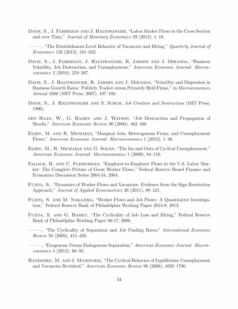
Davis, S., J. Faberman and J. Haltiwanger, “Labor Market Flows in the Cross Sectionand over Time,” Journal of Monetary Economics 59 (2012), 1–18.

———, “The Establishment-Level Behavior of Vacancies and Hiring,” Quarterly Journal ofEconomics 128 (2013), 581–622.

Davis, S., J. Faberman, J. Haltiwanger, R. Jarmin and J. Miranda, “BusinessVolatility, Job Destruction, and Unemployment,” American Economic Journal: Macroe-conomics 2 (2010), 259–287.

Davis, S., J. Haltiwanger, R. Jarmin and J. Miranda, “Volatility and Dispersion inBusiness Growth Rates: Publicly Traded versus Privately Held Firms,” in MacroeconomicsAnnual 2006 (MIT Press, 2007), 107–180.

Davis, S., J. Haltiwanger and S. Schuh, Job Creation and Destruction (MIT Press,1996).

den Haan, W., G. Ramey and J. Watson, “Job Destruction and Propagation ofShocks,” American Economic Review 90 (2000), 482–498.

Elsby, M. and R. Michaels, “Marginal Jobs, Heterogenous Firms, and UnemploymentFlows,” American Economic Journal: Macroeconomics 1 (2013), 1–48.

Elsby, M., R. Michaels and G. Solon, “The Ins and Outs of Cyclical Unemployment,”American Economic Journal: Macroeconomics 1 (2009), 84–110.

Fallick, B. and C. Fleischman, “Employer-to-Employer Flows in the U.S. Labor Mar-ket: The Complete Picture of Gross Worker Flows,” Federal Reserve Board Finance andEconomics Discussion Series 2004-34, 2004.

Fujita, S., “Dynamics of Worker Flows and Vacancies: Evidence from the Sign RestrictionApproach,” Journal of Applied Econometrics 26 (2011), 89–121.

Fujita, S. and M. Nakajima, “Worker Flows and Job Flows: A Quantitative Investiga-tion,” Federal Reserve Bank of Philadelphia Working Paper 2013-9, 2013.

Fujita, S. and G. Ramey, “The Cyclicality of Job Loss and Hiring,” Federal ReserveBank of Philadelphia Working Paper 06-17, 2006.

———, “The Cyclicality of Separation and Job Finding Rates,” International EconomicReview 50 (2009), 415–430.

———, “Exogenous Versus Endogenous Separation,” American Economic Journal: Macroe-conomics 4 (2012), 68–93.

Hagedorn, M. and I. Manovskii, “The Cyclical Behavior of Equilibrium Unemploymentand Vacancies Revisited,” American Economic Review 98 (2008), 1692–1706.

34

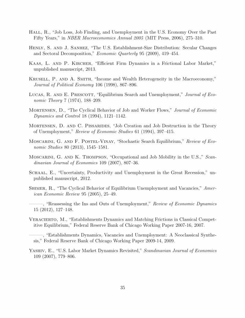
Hall, R., “Job Loss, Job Finding, and Unemployment in the U.S. Economy Over the PastFifty Years,” in NBER Macroeconomics Annual 2005 (MIT Press, 2006), 275–310.

Henly, S. and J. Sanhez, “The U.S. Establishment-Size Distribution: Secular Changesand Sectoral Decomposition,” Economic Quarterly 95 (2009), 419–454.

Kaas, L. and P. Kircher, “Efficient Firm Dynamics in a Frictional Labor Market,”unpublished manuscript, 2013.

Krusell, P. and A. Smith, “Income and Wealth Heterogeneity in the Macroeconomy,”Journal of Political Economy 106 (1998), 867–896.

Lucas, R. and E. Prescott, “Equilibrium Search and Unemployment,” Journal of Eco-nomic Theory 7 (1974), 188–209.

Mortensen, D., “The Cyclical Behavior of Job and Worker Flows,” Journal of EconomicDynamics and Control 18 (1994), 1121–1142.

Mortensen, D. and C. Pissarides, “Job Creation and Job Destruction in the Theoryof Unemployment,” Review of Economic Studies 61 (1994), 397–415.

Moscarini, G. and F. Postel-Vinay, “Stochastic Search Equilibrium,” Review of Eco-nomic Studies 80 (2013), 1545–1581.

Moscarini, G. and K. Thompson, “Occupational and Job Mobility in the U.S.,” Scan-dinavian Journal of Economics 109 (2007), 807–36.

Schaal, E., “Uncertainty, Productivity and Unemployment in the Great Recession,” un-published manuscript, 2012.

Shimer, R., “The Cyclical Behavior of Equilibrium Unemployment and Vacancies,” Amer-ican Economic Review 95 (2005), 25–49.

———, “Reassessing the Ins and Outs of Unemployment,” Review of Economic Dynamics15 (2012), 127–148.

Veracierto, M., “Establishments Dynamics and Matching Frictions in Classical Compet-itive Equilibrium,” Federal Reserve Bank of Chicago Working Paper 2007-16, 2007.

———, “Establishments Dynamics, Vacancies and Unemployment: A Neoclassical Synthe-sis,” Federal Reserve Bank of Chicago Working Paper 2009-14, 2009.

Yashiv, E., “U.S. Labor Market Dynamics Revisited,” Scandinavian Journal of Economics109 (2007), 779–806.

35