Embed Size (px)
Citation preview
1
Workflow for import, SCI inversion, visualization, interpretation and presentation of SPIA TEM inversions in Aarhus Workbench
This guide presents some of the common options from workspace creation to final presentation of data for
SPIA TEM data in Aarhus workbench. Aarhus Workbench contains a wealth of options and possibilities and
not all of them are presented in this manual, but all the basic options and many of the advanced options
related to working with ground based TEM data are presented.
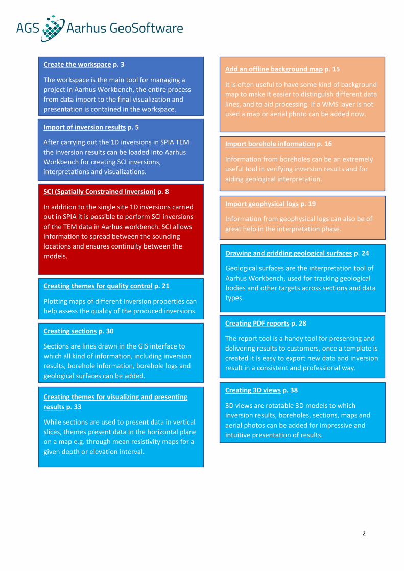
The flowchart is color-coded, the deep blue boxes are the core task that will always be carried out, the
ordering is to start from the top and work downwards. The orange boxes are optional extras that can be
carried out if the relevant data are available. The light blue boxes are quality control and presentation tasks
of which a few are usually carried out. One special option for inversion results imported from SPIA is to
perform a SCI inversion of the data, shown as a red box.
If viewed as a PDF the headers of the different boxes are links that will take you to the relevant guide, if
viewed in print you will have to navigate to the page number next to the title in each box.
Further information Within Workbench, it is always possible to press F1 to get help about the active window. This will open the
relevant help page from our online wiki page.
For advanced features, data examples, etc. go to our main wiki page:
http://www.ags-cloud.dk/Wiki/Workbench
This main page can also be accessed from within Workbench by pressing File –> help.
2
Create the workspace p. 3
The workspace is the main tool for managing a
project in Aarhus Workbench, the entire process
from data import to the final visualization and
presentation is contained in the workspace.
Import of inversion results p. 5
After carrying out the 1D inversions in SPIA TEM
the inversion results can be loaded into Aarhus
Workbench for creating SCI inversions,
interpretations and visualizations.
Add an offline background map p. 15
It is often useful to have some kind of background
map to make it easier to distinguish different data
lines, and to aid processing. If a WMS layer is not
used a map or aerial photo can be added now.
Import borehole information p. 16
Information from boreholes can be an extremely
useful tool in verifying inversion results and for
aiding geological interpretation.
SCI (Spatially Constrained Inversion) p. 8
In addition to the single site 1D inversions carried
out in SPIA it is possible to perform SCI inversions
of the TEM data in Aarhus workbench. SCI allows
information to spread between the sounding
locations and ensures continuity between the
models.
Creating sections p. 30
Sections are lines drawn in the GIS interface to
which all kind of information, including inversion
results, borehole information, borehole logs and
geological surfaces can be added.
Creating 3D views p. 38
3D views are rotatable 3D models to which
inversion results, boreholes, sections, maps and
aerial photos can be added for impressive and
intuitive presentation of results.
Creating PDF reports p. 28
The report tool is a handy tool for presenting and
delivering results to customers, once a template is
created it is easy to export new data and inversion
result in a consistent and professional way.
Import geophysical logs p. 19
Information from geophysical logs can also be of
great help in the interpretation phase.
Creating themes for quality control p. 21
Plotting maps of different inversion properties can
help assess the quality of the produced inversions.
Creating themes for visualizing and presenting
results p. 33
While sections are used to present data in vertical
slices, themes present data in the horizontal plane
on a map e.g. through mean resistivity maps for a
given depth or elevation interval.
Drawing and gridding geological surfaces p. 24
Geological surfaces are the interpretation tool of
Aarhus Workbench, used for tracking geological
bodies and other targets across sections and data
types.
3
Creating a workspace The first thing to do in any workbench project is to create the workspace. The workspace is the main
project wrapper; a single workspace is often enough to handle an entire project. The workspace can
contain geophysical data from different instruments, borehole information, maps, inversions, visualizations
and basic geological interpretations.
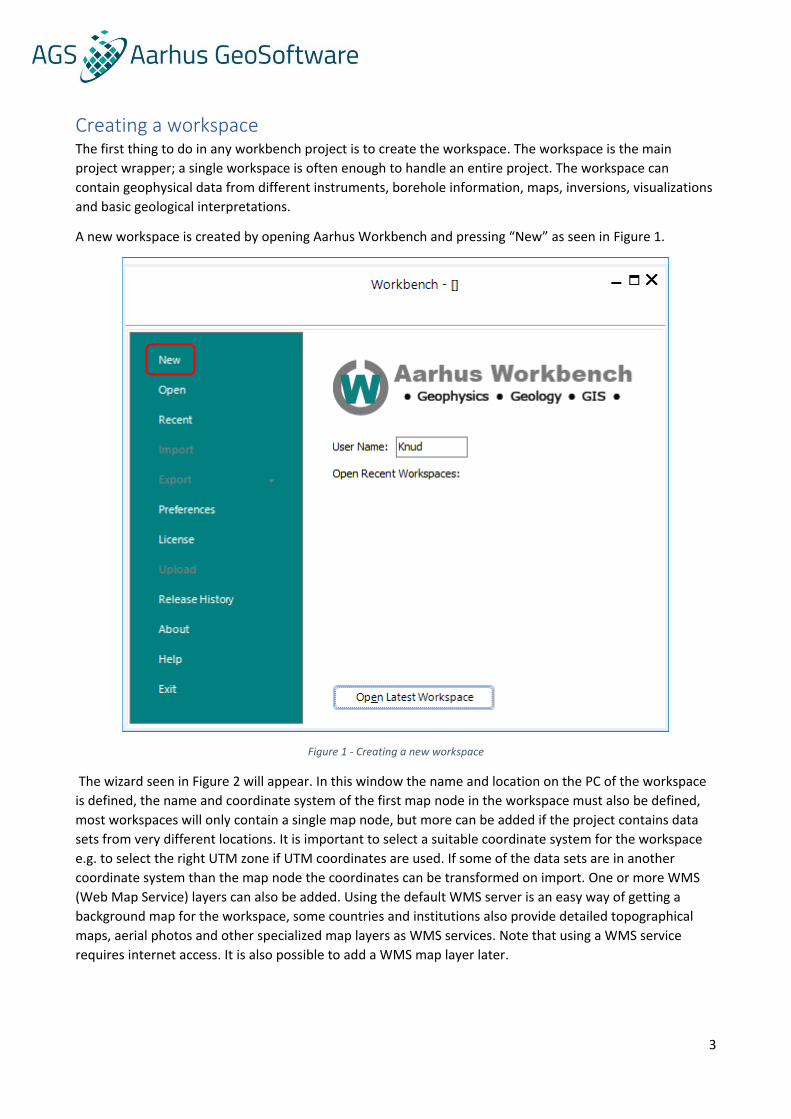
A new workspace is created by opening Aarhus Workbench and pressing “New” as seen in Figure 1.
Figure 1 - Creating a new workspace
The wizard seen in Figure 2 will appear. In this window the name and location on the PC of the workspace
is defined, the name and coordinate system of the first map node in the workspace must also be defined,
most workspaces will only contain a single map node, but more can be added if the project contains data
sets from very different locations. It is important to select a suitable coordinate system for the workspace
e.g. to select the right UTM zone if UTM coordinates are used. If some of the data sets are in another
coordinate system than the map node the coordinates can be transformed on import. One or more WMS
(Web Map Service) layers can also be added. Using the default WMS server is an easy way of getting a
background map for the workspace, some countries and institutions also provide detailed topographical
maps, aerial photos and other specialized map layers as WMS services. Note that using a WMS service
requires internet access. It is also possible to add a WMS map layer later.
4
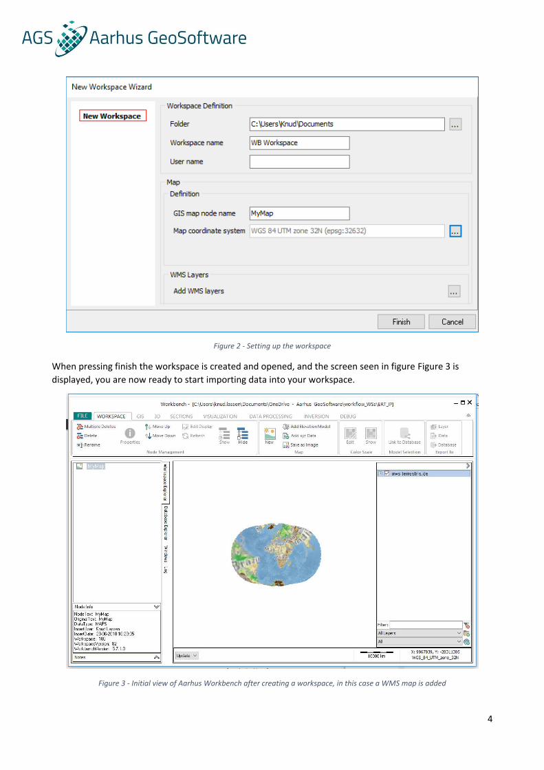
Figure 2 - Setting up the workspace
When pressing finish the workspace is created and opened, and the screen seen in figure Figure 3 is
displayed, you are now ready to start importing data into your workspace.
Figure 3 - Initial view of Aarhus Workbench after creating a workspace, in this case a WMS map is added
5
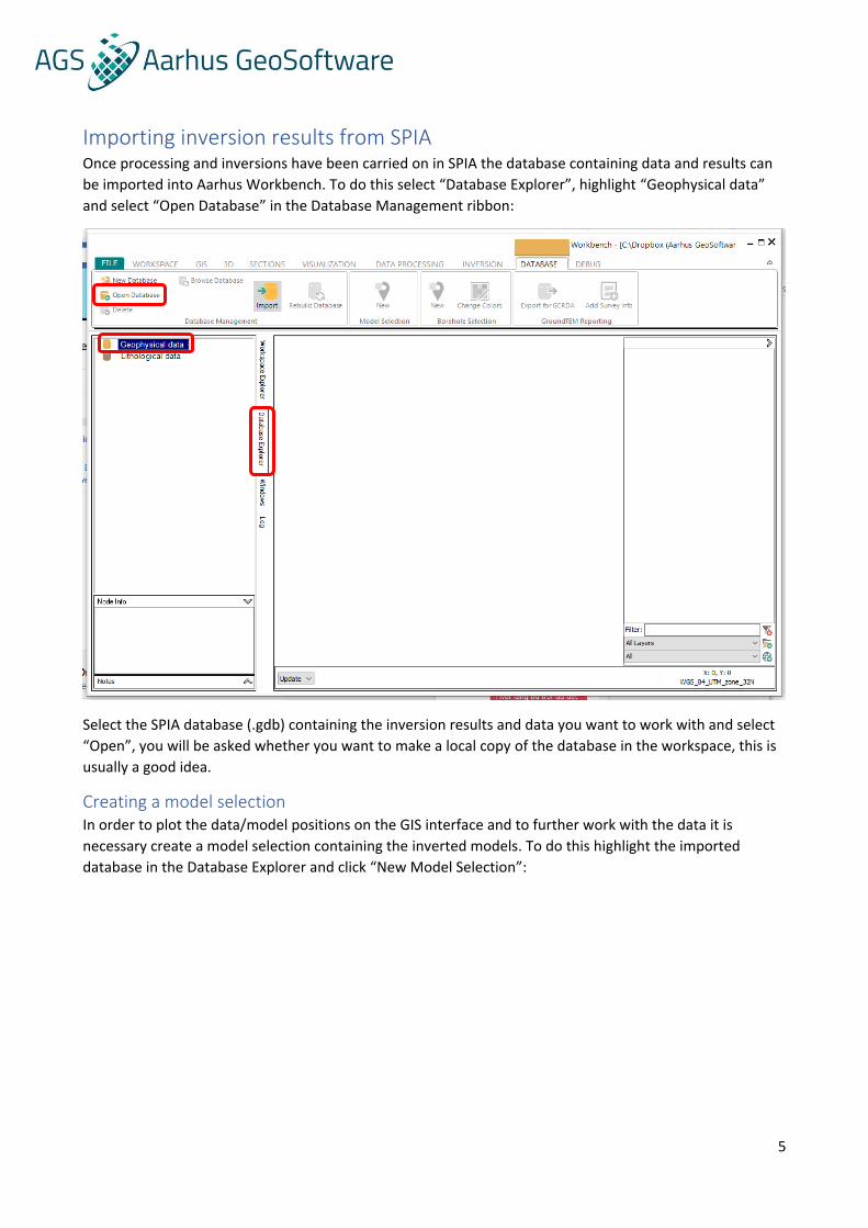
Importing inversion results from SPIA Once processing and inversions have been carried on in SPIA the database containing data and results can
be imported into Aarhus Workbench. To do this select “Database Explorer”, highlight “Geophysical data”
and select “Open Database” in the Database Management ribbon:
Select the SPIA database (.gdb) containing the inversion results and data you want to work with and select
“Open”, you will be asked whether you want to make a local copy of the database in the workspace, this is
usually a good idea.
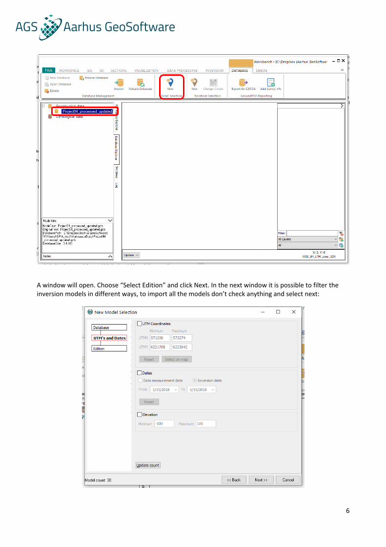
Creating a model selection In order to plot the data/model positions on the GIS interface and to further work with the data it is
necessary create a model selection containing the inverted models. To do this highlight the imported
database in the Database Explorer and click “New Model Selection”:
6
A window will open. Choose “Select Edition” and click Next. In the next window it is possible to filter the inversion models in different ways, to import all the models don’t check anything and select next:
7
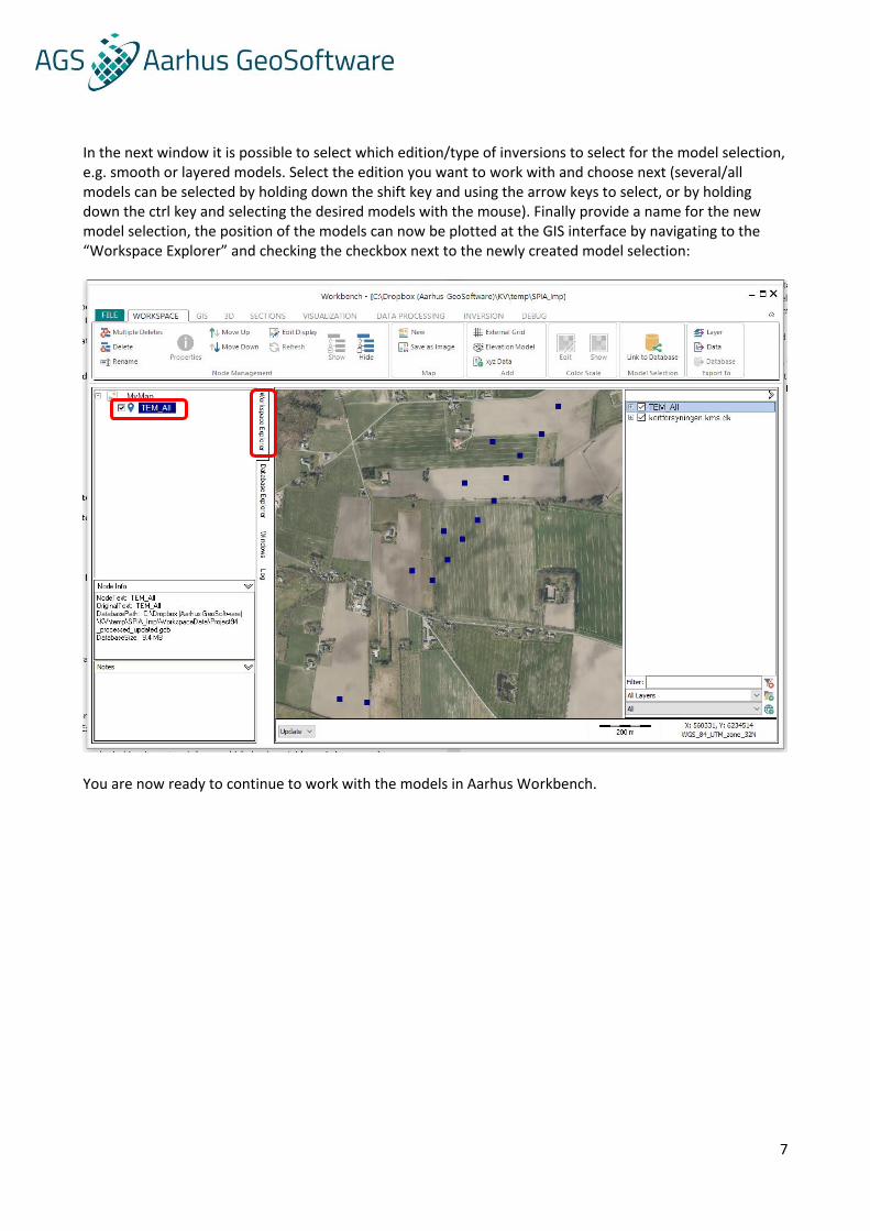
In the next window it is possible to select which edition/type of inversions to select for the model selection, e.g. smooth or layered models. Select the edition you want to work with and choose next (several/all models can be selected by holding down the shift key and using the arrow keys to select, or by holding down the ctrl key and selecting the desired models with the mouse). Finally provide a name for the new model selection, the position of the models can now be plotted at the GIS interface by navigating to the “Workspace Explorer” and checking the checkbox next to the newly created model selection:
You are now ready to continue to work with the models in Aarhus Workbench.
8
Performing an SCI inversion of the imported data
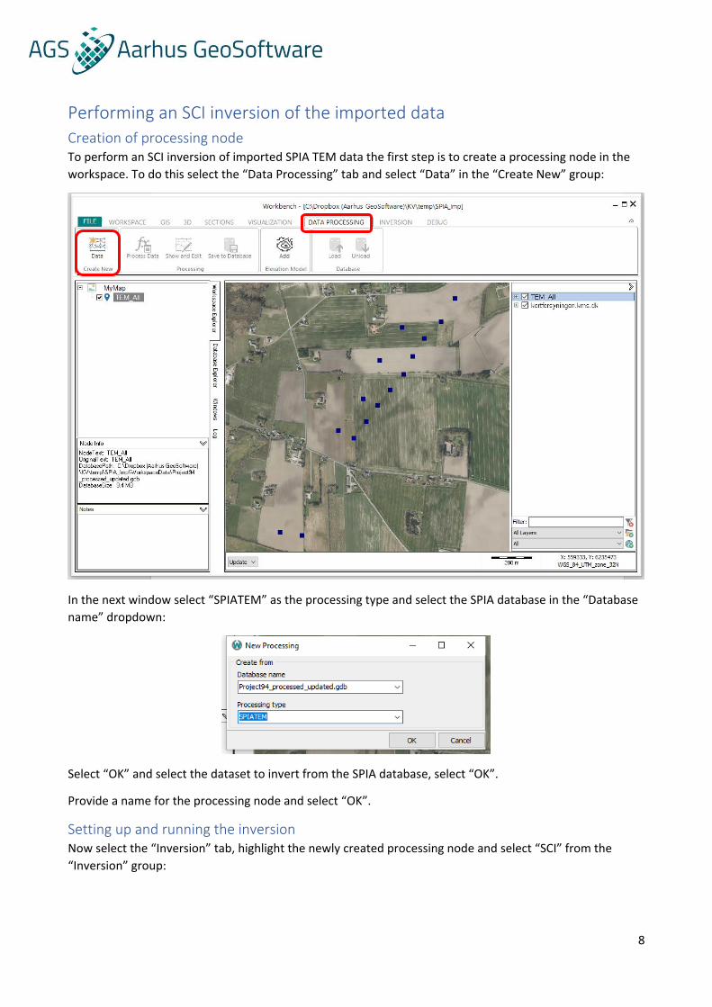
Creation of processing node To perform an SCI inversion of imported SPIA TEM data the first step is to create a processing node in the
workspace. To do this select the “Data Processing” tab and select “Data” in the “Create New” group:
In the next window select “SPIATEM” as the processing type and select the SPIA database in the “Database
name” dropdown:
Select “OK” and select the dataset to invert from the SPIA database, select “OK”.
Provide a name for the processing node and select “OK”.
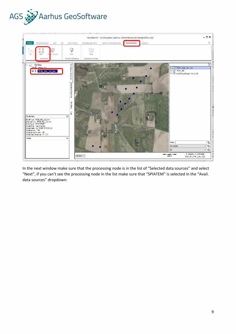
Setting up and running the inversion Now select the “Inversion” tab, highlight the newly created processing node and select “SCI” from the
“Inversion” group:
9
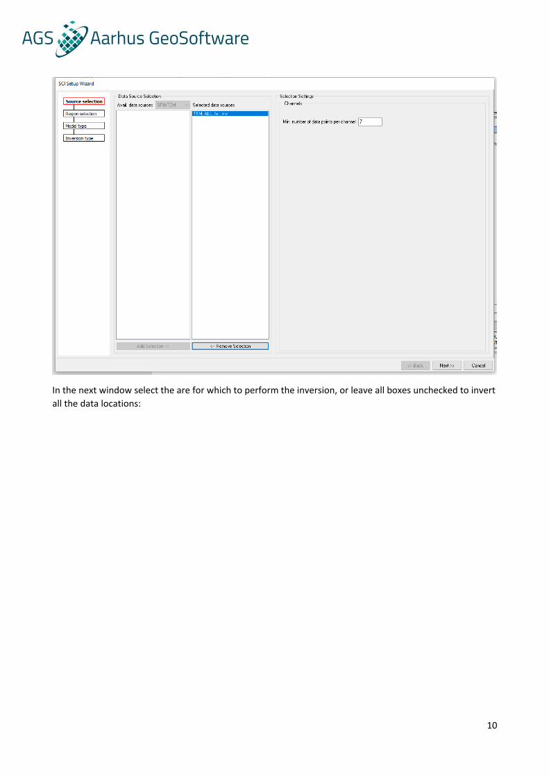
In the next window make sure that the processing node is in the list of “Selected data sources” and select
“Next”, if you can’t see the processing node in the list make sure that “SPIATEM” is selected in the “Avail.
data sources” dropdown:
10
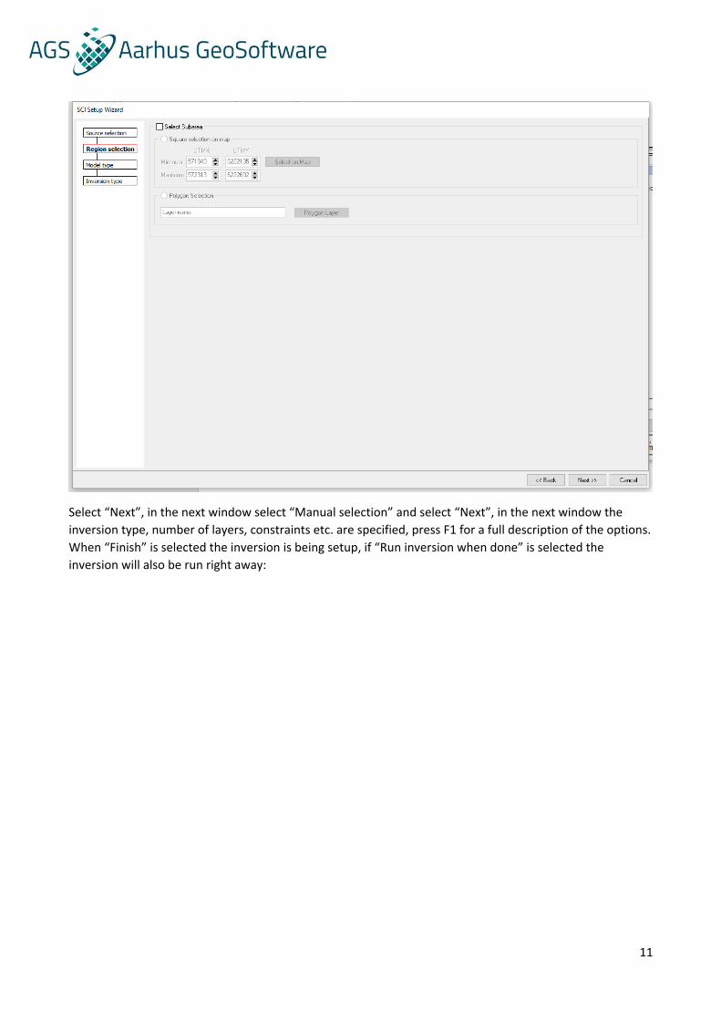
In the next window select the are for which to perform the inversion, or leave all boxes unchecked to invert
all the data locations:
11
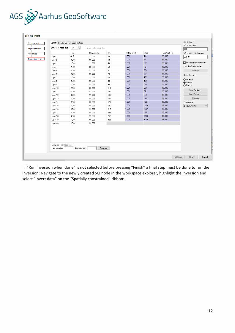
Select “Next”, in the next window select “Manual selection” and select “Next”, in the next window the
inversion type, number of layers, constraints etc. are specified, press F1 for a full description of the options.
When “Finish” is selected the inversion is being setup, if “Run inversion when done” is selected the
inversion will also be run right away:
12
If “Run inversion when done” is not selected before pressing “Finish” a final step must be done to run the
inversion: Navigate to the newly created SCI node in the workspace explorer, highlight the inversion and
select “Invert data” on the “Spatially constrained” ribbon:
13
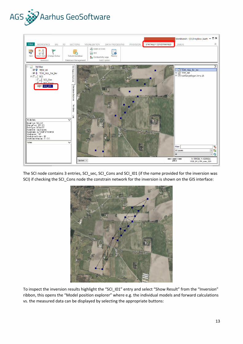
The SCI node contains 3 entries, SCI_sec, SCI_Cons and SCI_I01 (if the name provided for the inversion was
SCI) if checking the SCI_Cons node the constrain network for the inversion is shown on the GIS interface:
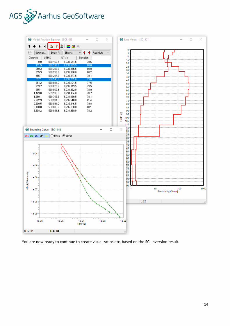
To inspect the inversion results highlight the “SCI_I01” entry and select “Show Result” from the “Inversion”
ribbon, this opens the “Model position explorer” where e.g. the individual models and forward calculations
vs. the measured data can be displayed by selecting the appropriate buttons:
14
You are now ready to continue to create visualizatios etc. based on the SCI inversion result.
15
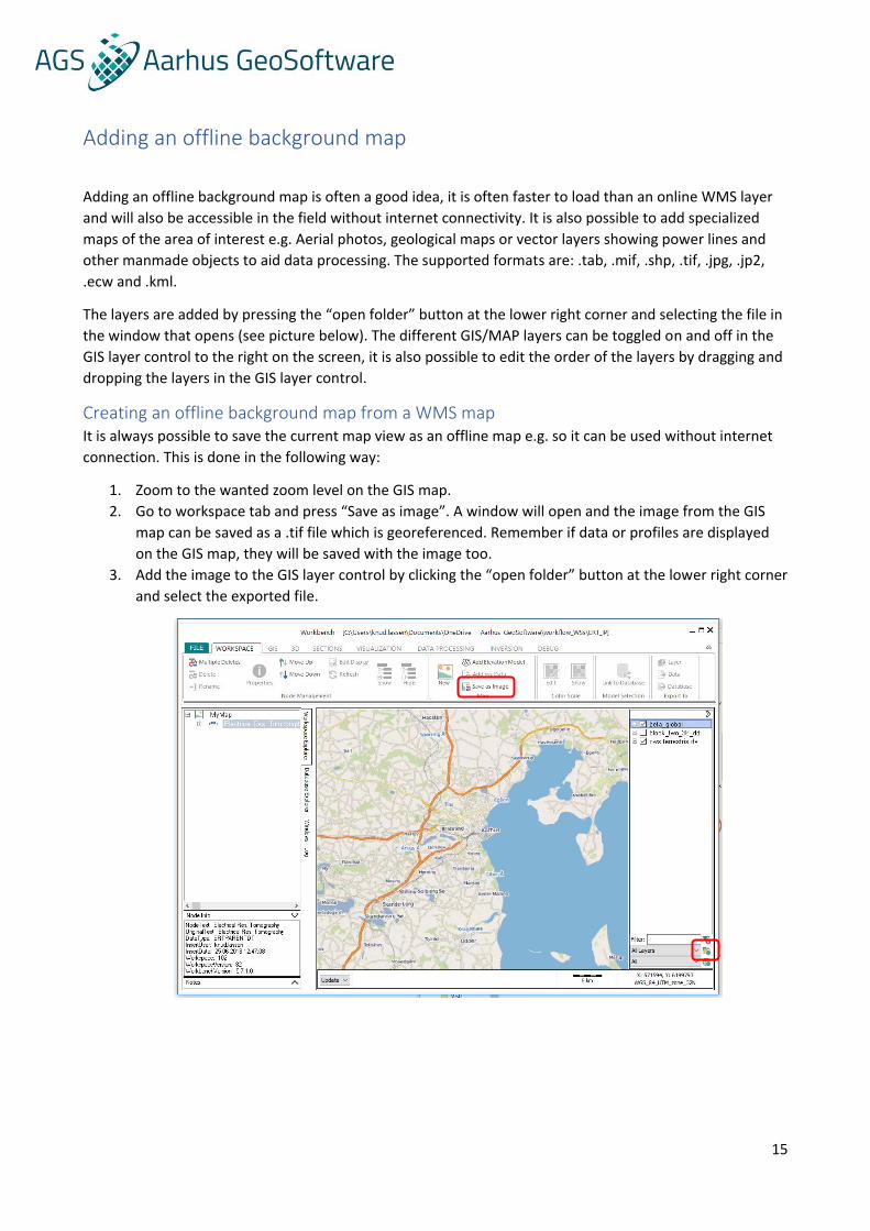
Adding an offline background map
Adding an offline background map is often a good idea, it is often faster to load than an online WMS layer
and will also be accessible in the field without internet connectivity. It is also possible to add specialized
maps of the area of interest e.g. Aerial photos, geological maps or vector layers showing power lines and
other manmade objects to aid data processing. The supported formats are: .tab, .mif, .shp, .tif, .jpg, .jp2,
.ecw and .kml.
The layers are added by pressing the “open folder” button at the lower right corner and selecting the file in
the window that opens (see picture below). The different GIS/MAP layers can be toggled on and off in the
GIS layer control to the right on the screen, it is also possible to edit the order of the layers by dragging and
dropping the layers in the GIS layer control.
Creating an offline background map from a WMS map It is always possible to save the current map view as an offline map e.g. so it can be used without internet
connection. This is done in the following way:
1. Zoom to the wanted zoom level on the GIS map.
2. Go to workspace tab and press “Save as image”. A window will open and the image from the GIS
map can be saved as a .tif file which is georeferenced. Remember if data or profiles are displayed
on the GIS map, they will be saved with the image too.
3. Add the image to the GIS layer control by clicking the “open folder” button at the lower right corner
and select the exported file.
16
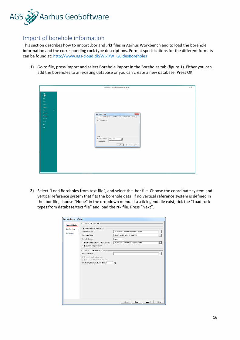
Import of borehole information This section describes how to import .bor and .rkt files in Aarhus Workbench and to load the borehole information and the corresponding rock type descriptions. Format specifications for the different formats can be found at: http://www.ags-cloud.dk/Wiki/W_GuidesBoreholes
1) Go to file, press import and select Borehole import in the Boreholes tab (figure 1). Either you can add the boreholes to an existing database or you can create a new database. Press OK.
2) Select “Load Boreholes from text file”, and select the .bor file. Choose the coordinate system and vertical reference system that fits the borehole data. If no vertical reference system is defined in the .bor file, choose ”None” in the dropdown menu. If a .rtk legend file exist, tick the “Load rock types from database/text file” and load the rtk file. Press “Next”.
17
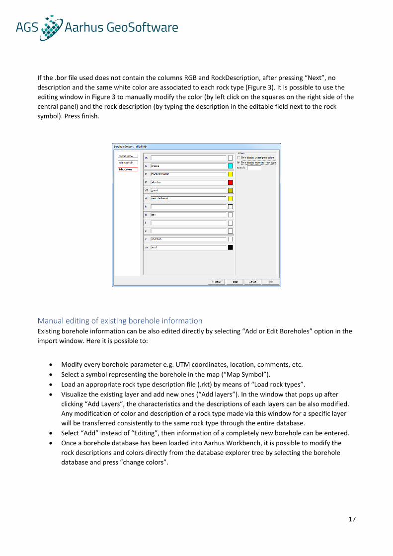
If the .bor file used does not contain the columns RGB and RockDescription, after pressing “Next”, no
description and the same white color are associated to each rock type (Figure 3). It is possible to use the
editing window in Figure 3 to manually modify the color (by left click on the squares on the right side of the
central panel) and the rock description (by typing the description in the editable field next to the rock
symbol). Press finish.
Manual editing of existing borehole information Existing borehole information can be also edited directly by selecting “Add or Edit Boreholes” option in the
import window. Here it is possible to:
• Modify every borehole parameter e.g. UTM coordinates, location, comments, etc.
• Select a symbol representing the borehole in the map (“Map Symbol”).
• Load an appropriate rock type description file (.rkt) by means of “Load rock types”.
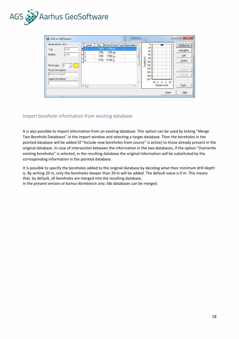
• Visualize the existing layer and add new ones (“Add layers”). In the window that pops up after
clicking “Add Layers”, the characteristics and the descriptions of each layers can be also modified.
Any modification of color and description of a rock type made via this window for a specific layer
will be transferred consistently to the same rock type through the entire database.
• Select “Add” instead of “Editing”, then information of a completely new borehole can be entered.
• Once a borehole database has been loaded into Aarhus Workbench, it is possible to modify the
rock descriptions and colors directly from the database explorer tree by selecting the borehole
database and press “change colors”.
18
Import borehole information from existing database
It is also possible to import information from an existing database. This option can be used by ticking “Merge
Two Borehole Databases” in the import window and selecting a target database. Then the boreholes in the
pointed database will be added (if “Include new boreholes from source” is active) to those already present in the
original database. In case of intersection between the information in the two databases, if the option “Overwrite
existing boreholes” is selected, in the resulting database the original information will be substituted by the
corresponding information in the pointed database.
It is possible to specify the boreholes added to the original database by deciding what their minimum drill depth is. By writing 20 m, only the boreholes deeper than 20 m will be added. The default value is 0 m. This means that, by default, all boreholes are merged into the resulting database. In the present version of Aarhus Workbench only .fdb databases can be merged.
19
Geophysical logs guide
This guide will go through import and display of geophysical logs in the .las 2.0 format. For more
information on the format go to http://www.cwls.org/las/
Data examples can be found at: http://www.ags-cloud.dk/Wiki/W_GuidesGeophysicalLogs
.las file criteria’s
Both wrapped and unwrapped format is supported. the minimum information needed in the .las file are:
~V /~Version header
Vers.
Wrap.
~W /~Well information
NULL.
X .M (F or FT). Coordinate system has to be UTM.
Y .M (F or FT). Coordinate system has to be UTM.
Z (for elevation - optional)
~C /~Curve information
DEPTH or DEPT (units have to be .M / .F /.FT)
Units
Curve description
~P /~Parameter information
Each line needs to contain a value for each unit
Import
1. Open Aarhus Workbench, open or create a workspace.
2. Go to the “Database Explorer”, highlight the “Geophysical data”, go to the “Database” ribbon and
click “Import”.
3. Select Boreholes → Geophysical Log import and choose which database (either existing or new) to
import the data into.
4. Add .las files to the importer, select the UTM zone of the UTM coordinates within the .las file.
5. If the UTM zone is different from the workspace, transform the coordinates into the correct UTM
zone.
6. Click import

20
Display geophysical logs
1. Go the “Database Explorer”, highlight the database that contains the data from the geophysical
logs. Go to the “Database” ribbon and click New Borehole Selection.
2. A Borehole Log Query will open. Press OK to get all logs selected and give the model selection a
name.
3. Go to the Workspace Explorer, expand the MyMap node and tick the box for the model selection.
The location of all the logs will be displayed on the GIS map.
4. Go to the “GIS” ribbon and select either one or more logs on the GIS map. Use the pointer or
Rectangle tool. The selection can be cleared by the clear button.
5. When the wanted logs are selected click the “Use Selection” button and click “Show data”.
6. A new window for each log selected will be opened.
21
Creating and using quality control themes Model quality themes are a tool for assessing the quality of inversions and data processing by plotting
different values on a color scale on the GIS maps.
Common values to plot for the QC is total residual, data residual and dept of investigation (DOI).
The residuals can be used to determine how well the inverted models fit the data in different parts of the
survey, bad data fit can indicate that the data are coupled, too noisy or that the inversion set-up isn’t well
suited for the geological setting, the data can then be reprocessed and/or reinverted in these areas, or it
can be kept in mind that models from the areas can’t be trusted for interpretation.
DOI can be used to determine whether the survey resolve the subsurface to a sufficient depth to serve the
surveys purpose, and to guide the interpretation of data.
For airborne surveys it is also common to plot the instrument altitude and the difference between
measured and inverted altitude. A high altitude e.g. when passing high trees or structure can explain a
higher residual that otherwise can’t be explained. The differences between measured and inverted altitude
can serve as an indicator for either bad altitude processing or other problems in the inversion.
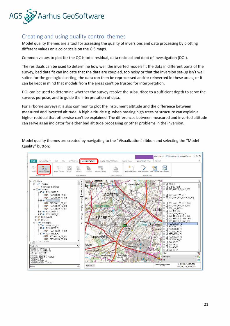
Model quality themes are created by navigating to the “Visualization” ribbon and selecting the “Model
Quality” button:
22
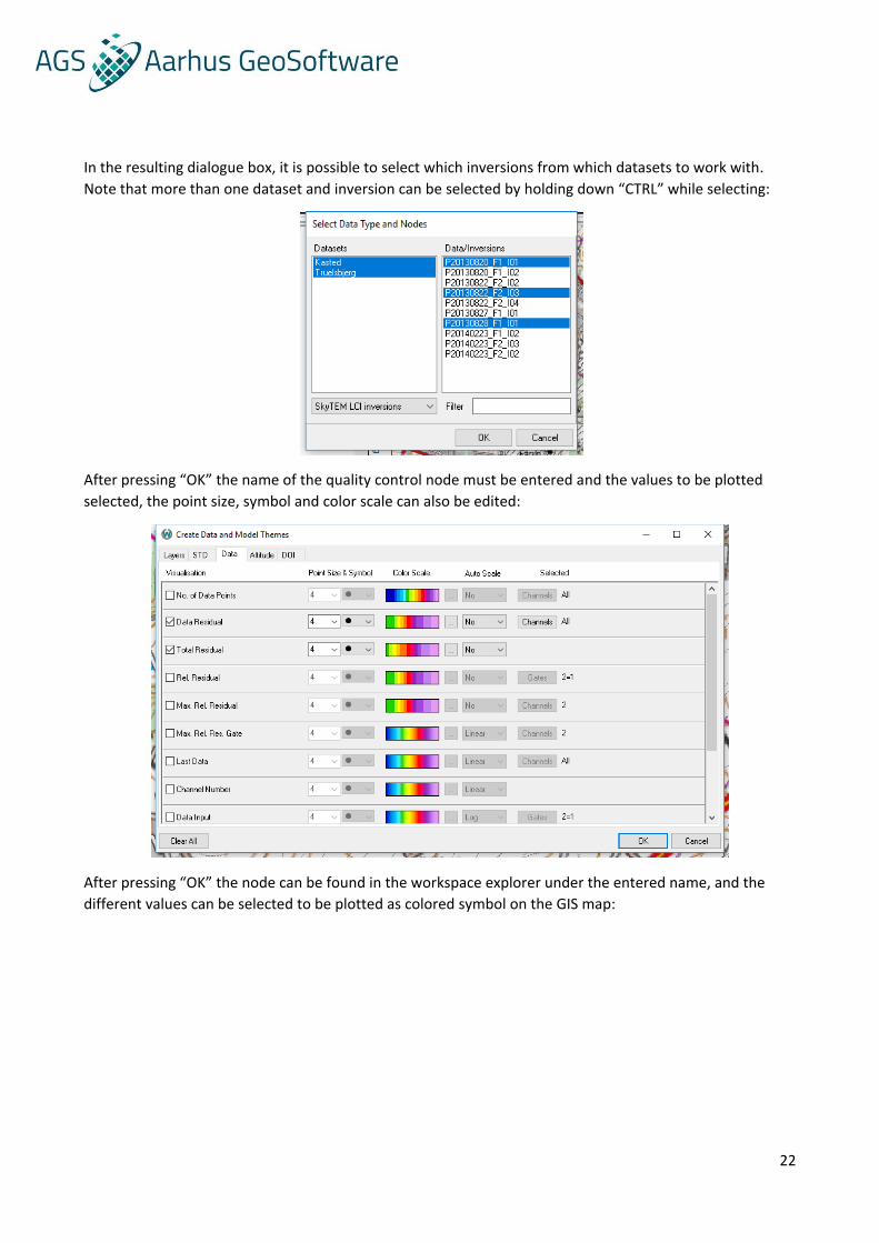
In the resulting dialogue box, it is possible to select which inversions from which datasets to work with.
Note that more than one dataset and inversion can be selected by holding down “CTRL” while selecting:
After pressing “OK” the name of the quality control node must be entered and the values to be plotted
selected, the point size, symbol and color scale can also be edited:
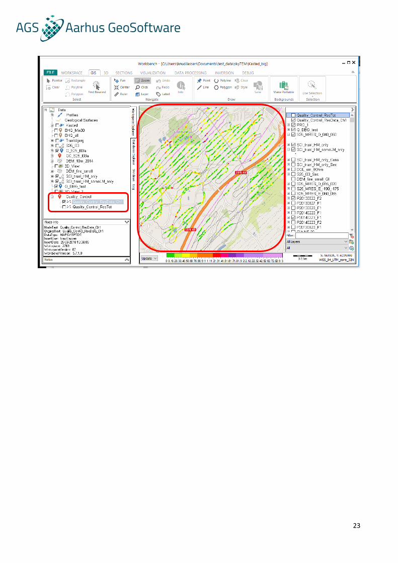
After pressing “OK” the node can be found in the workspace explorer under the entered name, and the
different values can be selected to be plotted as colored symbol on the GIS map:
23
24
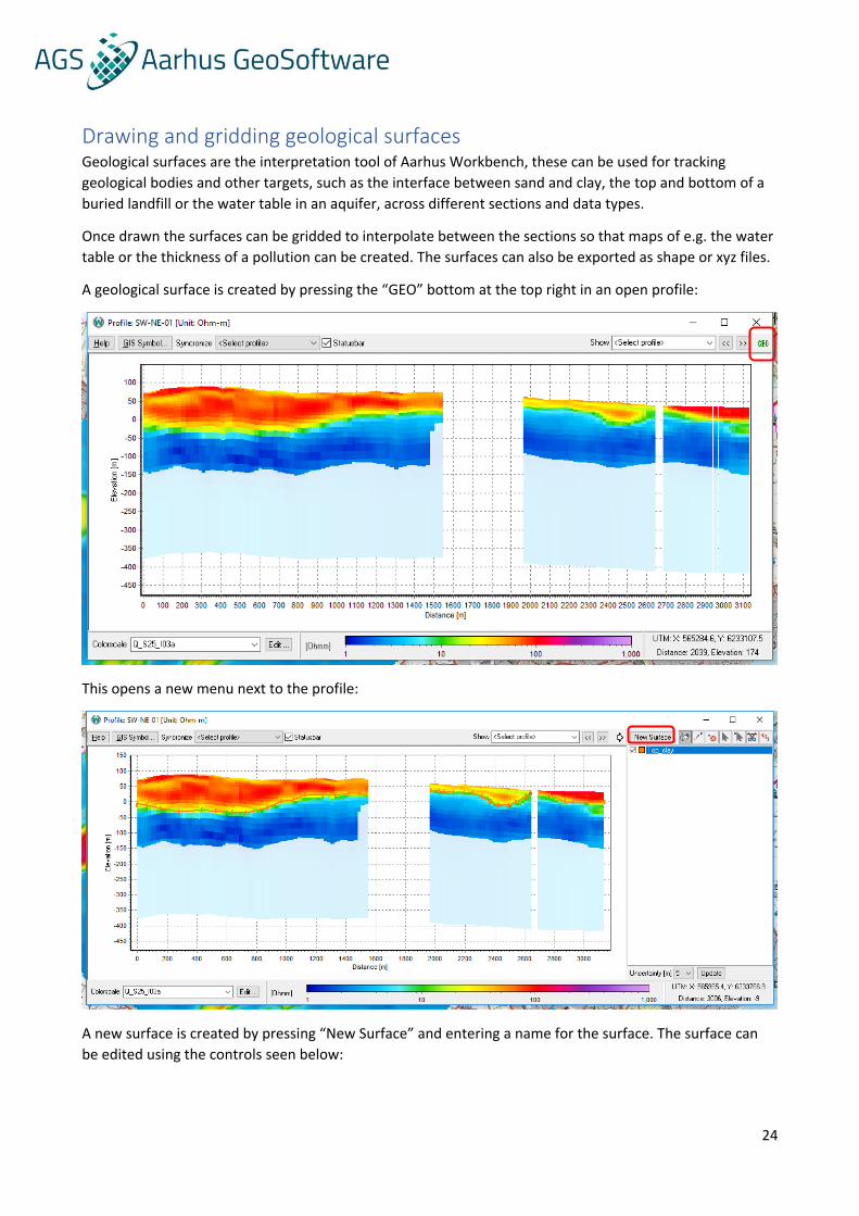
Drawing and gridding geological surfaces Geological surfaces are the interpretation tool of Aarhus Workbench, these can be used for tracking
geological bodies and other targets, such as the interface between sand and clay, the top and bottom of a
buried landfill or the water table in an aquifer, across different sections and data types.
Once drawn the surfaces can be gridded to interpolate between the sections so that maps of e.g. the water
table or the thickness of a pollution can be created. The surfaces can also be exported as shape or xyz files.
A geological surface is created by pressing the “GEO” bottom at the top right in an open profile:
This opens a new menu next to the profile:
A new surface is created by pressing “New Surface” and entering a name for the surface. The surface can
be edited using the controls seen below:
25
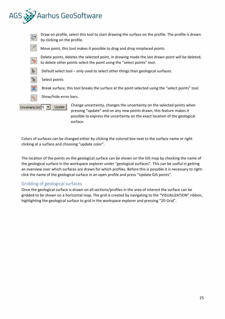
Draw on profile, select this tool to start drawing the surface on the profile. The profile is drawn
by clicking on the profile.
Move point, this tool makes it possible to drag and drop misplaced points
Delete points, deletes the selected point, in drawing mode the last drawn point will be deleted,
to delete other points select the point using the “select points” tool.
Default select tool – only used to select other things than geological surfaces.
Select points
Break surface, this tool breaks the surface at the point selected using the “select points” tool.
Show/hide error bars.
Change uncertainty, changes the uncertainty on the selected points when
pressing “update” and on any new points drawn, this feature makes it
possible to express the uncertainty on the exact location of the geological
surface.
Colors of surfaces can be changed either by clicking the colored box next to the surface name or right
clicking at a surface and choosing “update color”.
The location of the points on the geological surface can be shown on the GIS map by checking the name of
the geological surface in the workspace explorer under “geological surfaces”. This can be useful in getting
an overview over which surfaces are drawn for which profiles. Before this is possible it is necessary to right-
click the name of the geological surface in an open profile and press “Update GIS points”.
Gridding of geological surfaces Once the geological surface is drawn on all sections/profiles in the area of interest the surface can be
gridded to be shown on a horizontal map. The grid is created by navigating to the “VISUALIZATION” ribbon,
highlighting the geological surface to grid in the workspace explorer and pressing “2D Grid”.
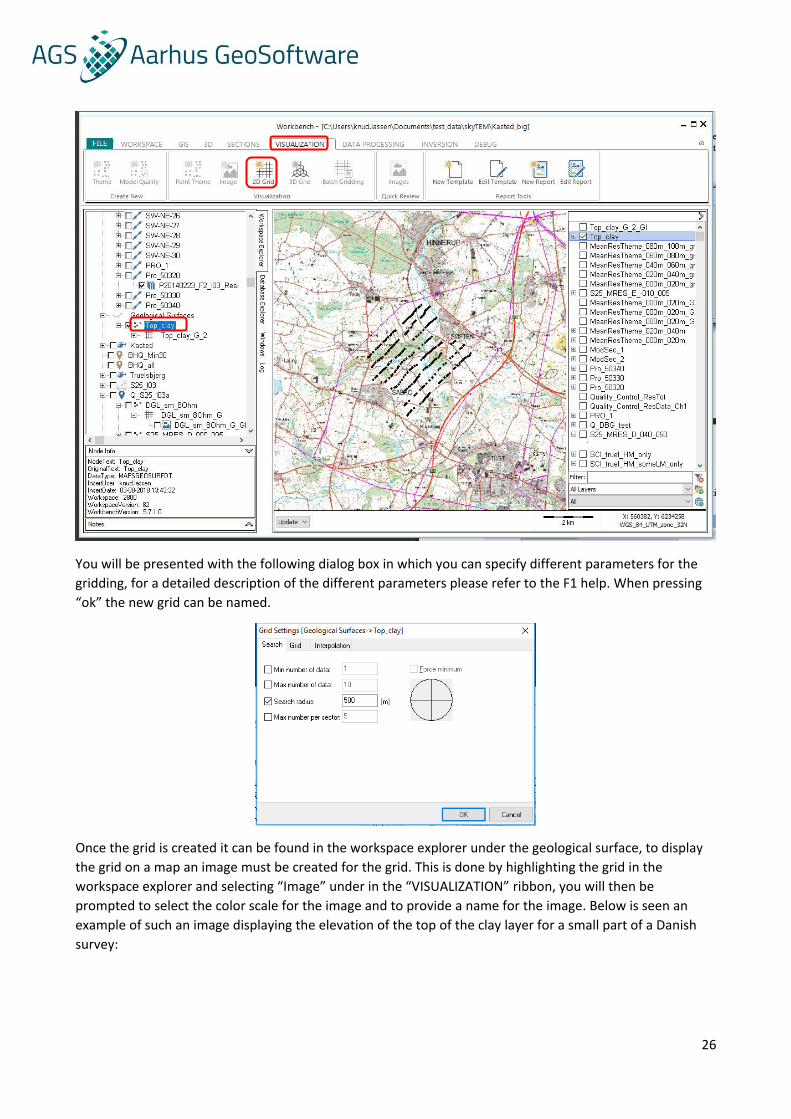
26
You will be presented with the following dialog box in which you can specify different parameters for the
gridding, for a detailed description of the different parameters please refer to the F1 help. When pressing
“ok” the new grid can be named.
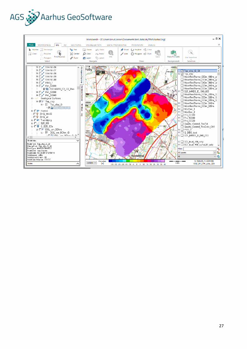
Once the grid is created it can be found in the workspace explorer under the geological surface, to display
the grid on a map an image must be created for the grid. This is done by highlighting the grid in the
workspace explorer and selecting “Image” under in the “VISUALIZATION” ribbon, you will then be
prompted to select the color scale for the image and to provide a name for the image. Below is seen an
example of such an image displaying the elevation of the top of the clay layer for a small part of a Danish
survey:
27
28
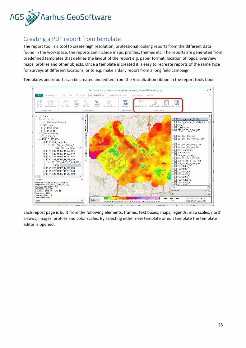
Creating a PDF report from template The report tool is a tool to create high resolution, professional looking reports from the different data
found in the workspace, the reports can include maps, profiles, themes etc. The reports are generated from
predefined templates that defines the layout of the report e.g. paper format, location of logos, overview
maps, profiles and other objects. Once a template is created it is easy to recreate reports of the same type
for surveys at different locations, or to e.g. make a daily report from a long field campaign.
Templates and reports can be created and edited from the Visualization ribbon in the report tools box:
Each report page is built from the following elements: frames, text boxes, maps, legends, map scales, north
arrows, images, profiles and color scales. By selecting either new template or edit template the template
editor is opened:
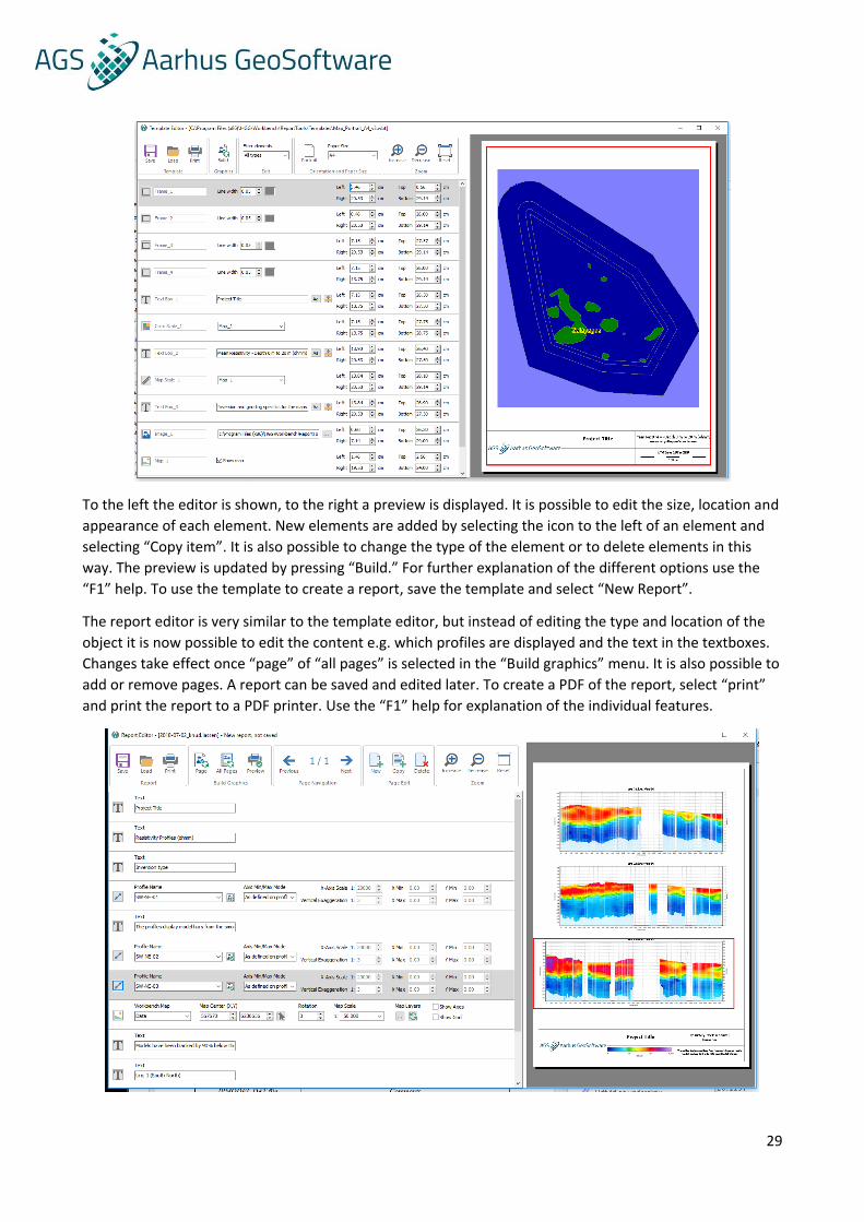
29
To the left the editor is shown, to the right a preview is displayed. It is possible to edit the size, location and
appearance of each element. New elements are added by selecting the icon to the left of an element and
selecting “Copy item”. It is also possible to change the type of the element or to delete elements in this
way. The preview is updated by pressing “Build.” For further explanation of the different options use the
“F1” help. To use the template to create a report, save the template and select “New Report”.
The report editor is very similar to the template editor, but instead of editing the type and location of the
object it is now possible to edit the content e.g. which profiles are displayed and the text in the textboxes.
Changes take effect once “page” of “all pages” is selected in the “Build graphics” menu. It is also possible to
add or remove pages. A report can be saved and edited later. To create a PDF of the report, select “print”
and print the report to a PDF printer. Use the “F1” help for explanation of the individual features.
30
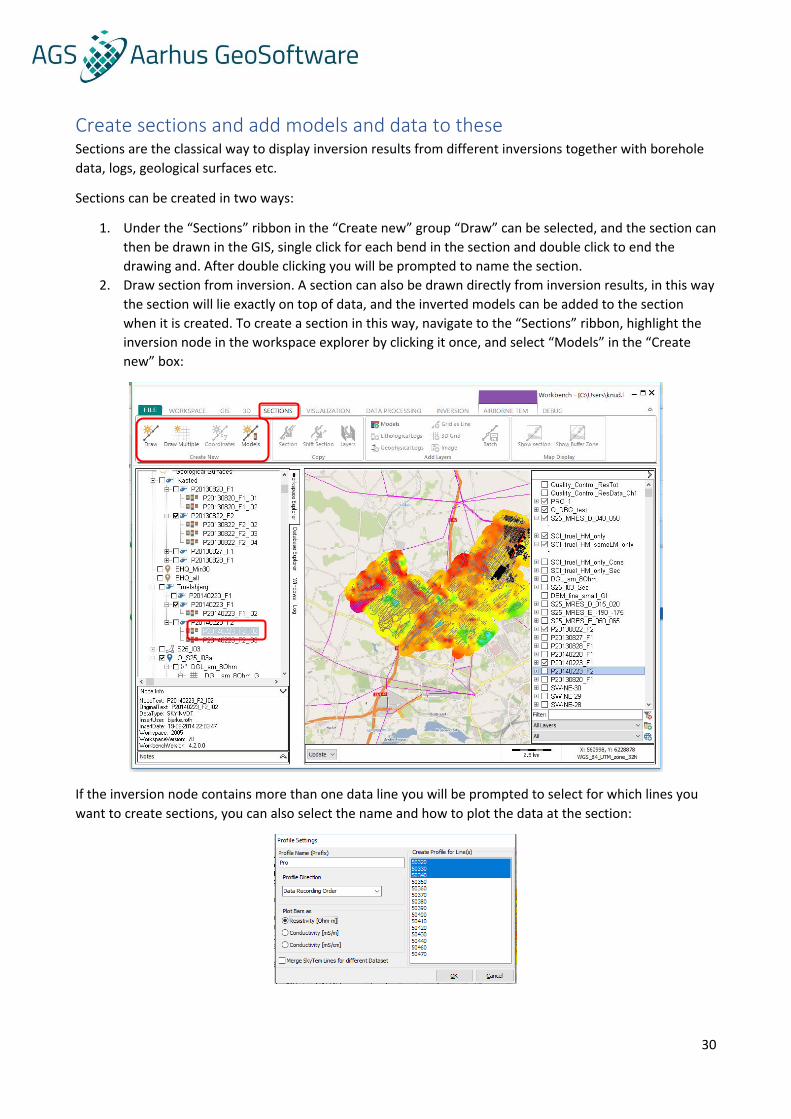
Create sections and add models and data to these Sections are the classical way to display inversion results from different inversions together with borehole
data, logs, geological surfaces etc.
Sections can be created in two ways:
1. Under the “Sections” ribbon in the “Create new” group “Draw” can be selected, and the section can
then be drawn in the GIS, single click for each bend in the section and double click to end the
drawing and. After double clicking you will be prompted to name the section.
2. Draw section from inversion. A section can also be drawn directly from inversion results, in this way
the section will lie exactly on top of data, and the inverted models can be added to the section
when it is created. To create a section in this way, navigate to the “Sections” ribbon, highlight the
inversion node in the workspace explorer by clicking it once, and select “Models” in the “Create
new” box:
If the inversion node contains more than one data line you will be prompted to select for which lines you
want to create sections, you can also select the name and how to plot the data at the section:
31
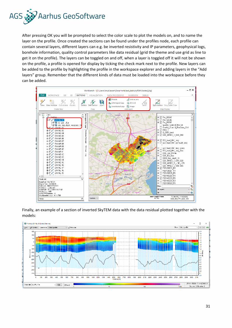
After pressing OK you will be prompted to select the color scale to plot the models on, and to name the
layer on the profile. Once created the sections can be found under the profiles node, each profile can
contain several layers, different layers can e.g. be inverted resistivity and IP parameters, geophysical logs,
borehole information, quality control parameters like data residual (grid the theme and use grid as line to
get it on the profile). The layers can be toggled on and off, when a layer is toggled off it will not be shown
on the profile, a profile is opened for display by ticking the check mark next to the profile. New layers can
be added to the profile by highlighting the profile in the workspace explorer and adding layers in the “Add
layers” group. Remember that the different kinds of data must be loaded into the workspace before they
can be added.
Finally, an example of a section of inverted SkyTEM data with the data residual plotted together with the
models:

32
Note that the range and type (logarithmic or linear) of the axis can be edited by double clicking the axis.
33
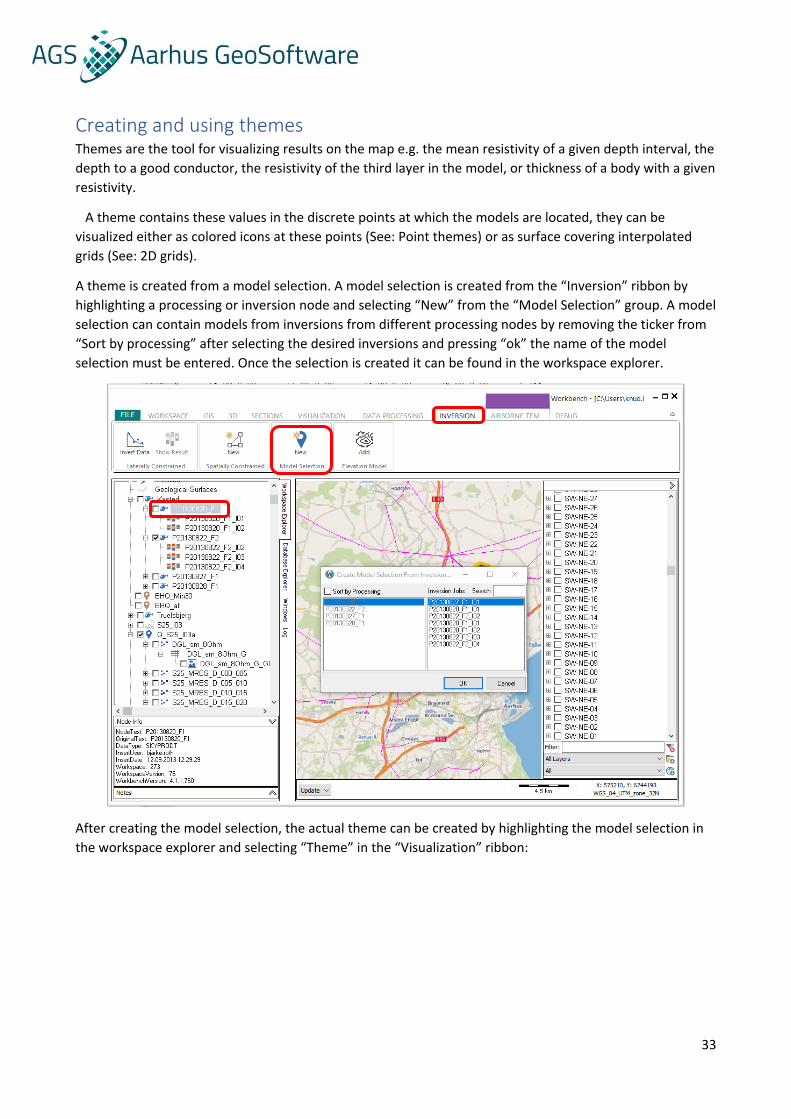
Creating and using themes Themes are the tool for visualizing results on the map e.g. the mean resistivity of a given depth interval, the
depth to a good conductor, the resistivity of the third layer in the model, or thickness of a body with a given
resistivity.
A theme contains these values in the discrete points at which the models are located, they can be
visualized either as colored icons at these points (See: Point themes) or as surface covering interpolated
grids (See: 2D grids).
A theme is created from a model selection. A model selection is created from the “Inversion” ribbon by
highlighting a processing or inversion node and selecting “New” from the “Model Selection” group. A model
selection can contain models from inversions from different processing nodes by removing the ticker from
“Sort by processing” after selecting the desired inversions and pressing “ok” the name of the model
selection must be entered. Once the selection is created it can be found in the workspace explorer.
After creating the model selection, the actual theme can be created by highlighting the model selection in
the workspace explorer and selecting “Theme” in the “Visualization” ribbon:
34
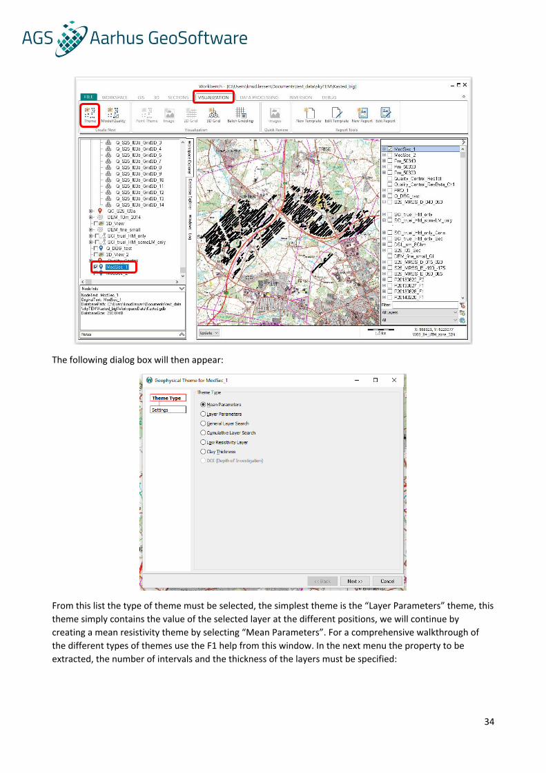
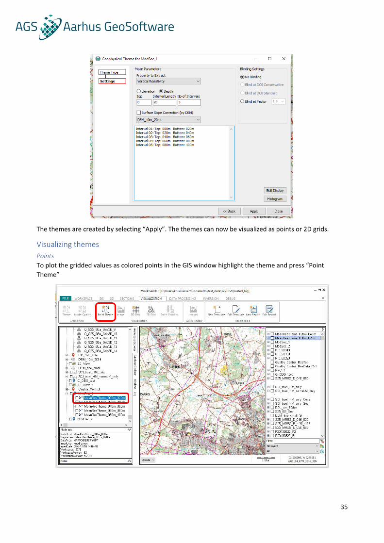
The following dialog box will then appear:
From this list the type of theme must be selected, the simplest theme is the “Layer Parameters” theme, this
theme simply contains the value of the selected layer at the different positions, we will continue by
creating a mean resistivity theme by selecting “Mean Parameters”. For a comprehensive walkthrough of
the different types of themes use the F1 help from this window. In the next menu the property to be
extracted, the number of intervals and the thickness of the layers must be specified:
35
The themes are created by selecting “Apply”. The themes can now be visualized as points or 2D grids.
Visualizing themes
Points
To plot the gridded values as colored points in the GIS window highlight the theme and press “Point
Theme”
36
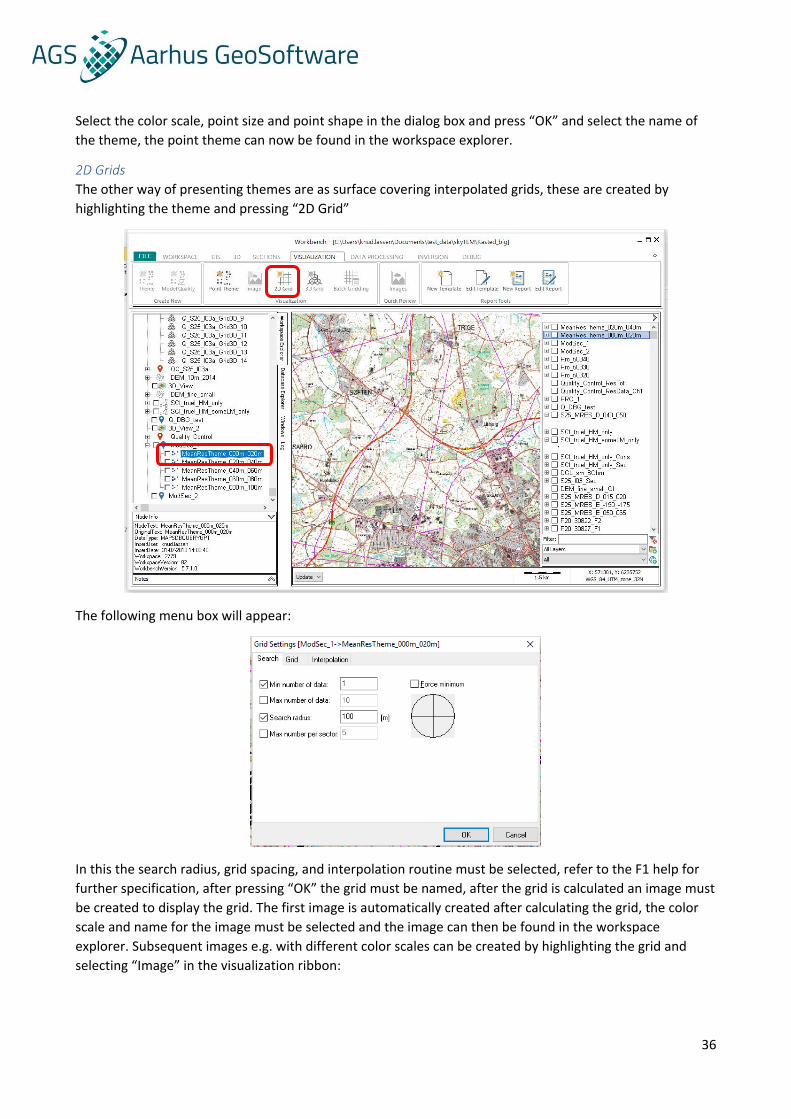
Select the color scale, point size and point shape in the dialog box and press “OK” and select the name of
the theme, the point theme can now be found in the workspace explorer.
2D Grids
The other way of presenting themes are as surface covering interpolated grids, these are created by
highlighting the theme and pressing “2D Grid”
The following menu box will appear:
In this the search radius, grid spacing, and interpolation routine must be selected, refer to the F1 help for
further specification, after pressing “OK” the grid must be named, after the grid is calculated an image must
be created to display the grid. The first image is automatically created after calculating the grid, the color
scale and name for the image must be selected and the image can then be found in the workspace
explorer. Subsequent images e.g. with different color scales can be created by highlighting the grid and
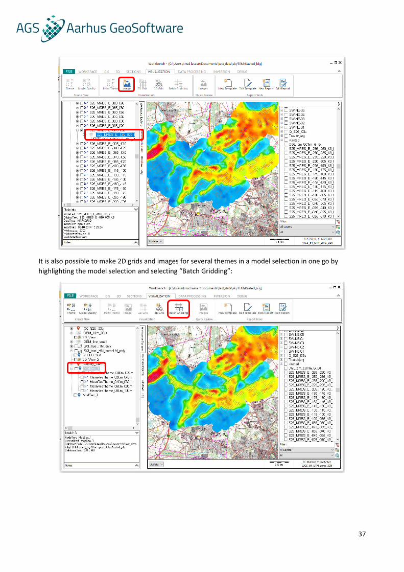
selecting “Image” in the visualization ribbon:
37
It is also possible to make 2D grids and images for several themes in a model selection in one go by
highlighting the model selection and selecting “Batch Gridding”:
38
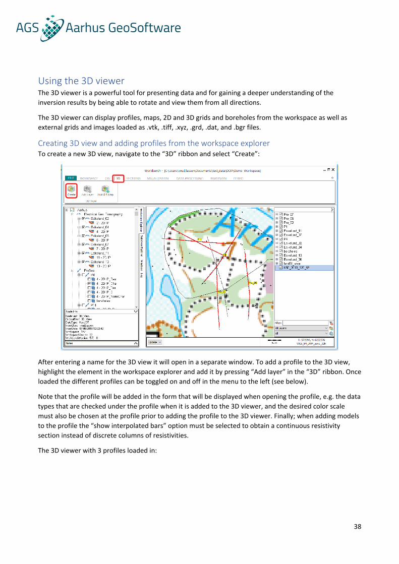
Using the 3D viewer The 3D viewer is a powerful tool for presenting data and for gaining a deeper understanding of the
inversion results by being able to rotate and view them from all directions.
The 3D viewer can display profiles, maps, 2D and 3D grids and boreholes from the workspace as well as
external grids and images loaded as .vtk, .tiff, .xyz, .grd, .dat, and .bgr files.
Creating 3D view and adding profiles from the workspace explorer To create a new 3D view, navigate to the “3D” ribbon and select “Create”:
After entering a name for the 3D view it will open in a separate window. To add a profile to the 3D view,
highlight the element in the workspace explorer and add it by pressing “Add layer” in the “3D” ribbon. Once
loaded the different profiles can be toggled on and off in the menu to the left (see below).
Note that the profile will be added in the form that will be displayed when opening the profile, e.g. the data
types that are checked under the profile when it is added to the 3D viewer, and the desired color scale
must also be chosen at the profile prior to adding the profile to the 3D viewer. Finally; when adding models
to the profile the “show interpolated bars” option must be selected to obtain a continuous resistivity
section instead of discrete columns of resistivities.
The 3D viewer with 3 profiles loaded in:
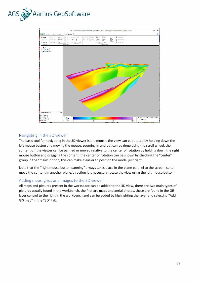
39
Navigating in the 3D viewer The basic tool for navigating in the 3D viewer is the mouse, the view can be rotated by holding down the
left mouse button and moving the mouse, zooming in and out can be done using the scroll wheel, the
content off the viewer can be panned or moved relative to the center of rotation by holding down the right
mouse button and dragging the content, the center of rotation can be shown by checking the “center”
group in the “main” ribbon, this can make it easier to position the model just right.
Note that the “right mouse button panning” always takes place in the plane parallel to the screen, so to
move the content in another plane/direction it is necessary rotate the view using the left mouse button.
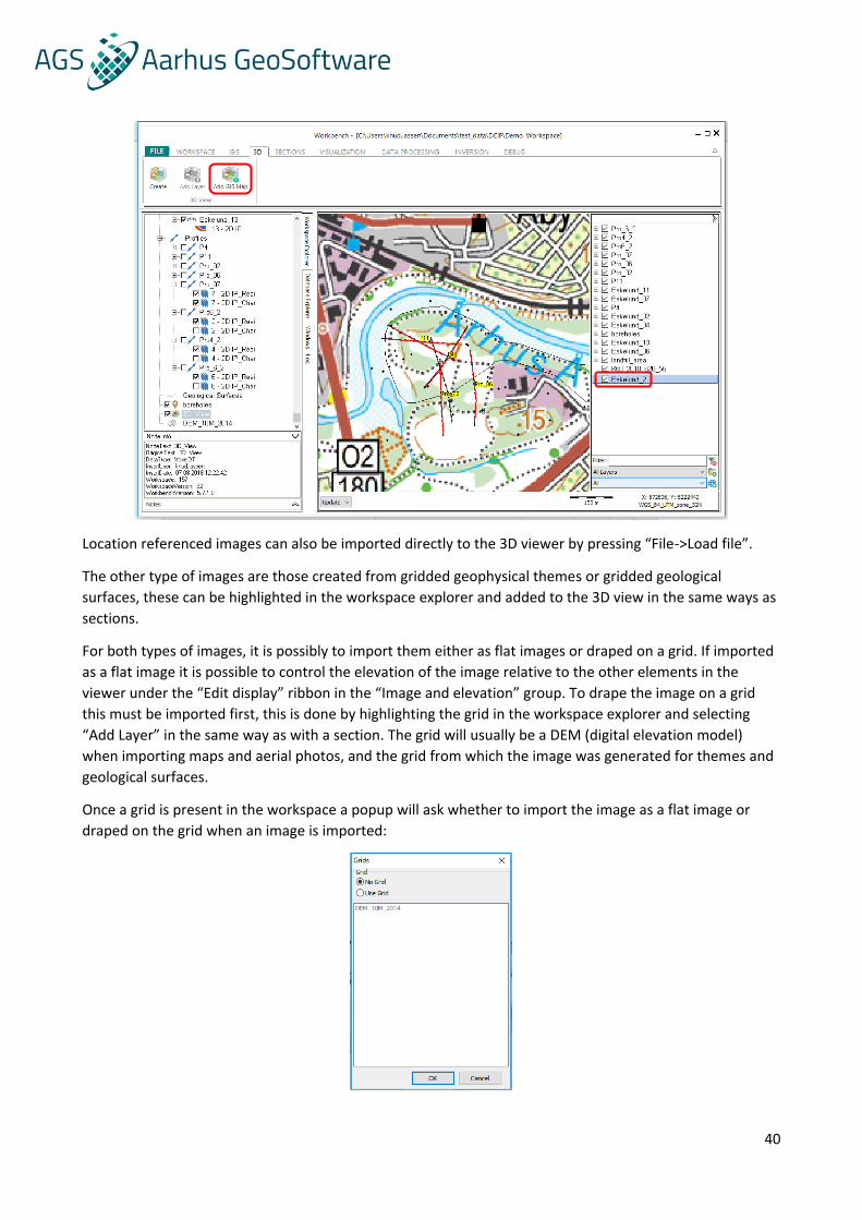
Adding maps, grids and images to the 3D viewer All maps and pictures present in the workspace can be added to the 3D view, there are two main types of
pictures usually found in the workbench, the first are maps and aerial photos, these are found in the GIS
layer control to the right in the workbench and can be added by highlighting the layer and selecting “Add
GIS map” in the “3D” tab:
40
Location referenced images can also be imported directly to the 3D viewer by pressing “File->Load file”.
The other type of images are those created from gridded geophysical themes or gridded geological
surfaces, these can be highlighted in the workspace explorer and added to the 3D view in the same ways as
sections.
For both types of images, it is possibly to import them either as flat images or draped on a grid. If imported
as a flat image it is possible to control the elevation of the image relative to the other elements in the
viewer under the “Edit display” ribbon in the “Image and elevation” group. To drape the image on a grid
this must be imported first, this is done by highlighting the grid in the workspace explorer and selecting
“Add Layer” in the same way as with a section. The grid will usually be a DEM (digital elevation model)
when importing maps and aerial photos, and the grid from which the image was generated for themes and
geological surfaces.
Once a grid is present in the workspace a popup will ask whether to import the image as a flat image or
draped on the grid when an image is imported:
41
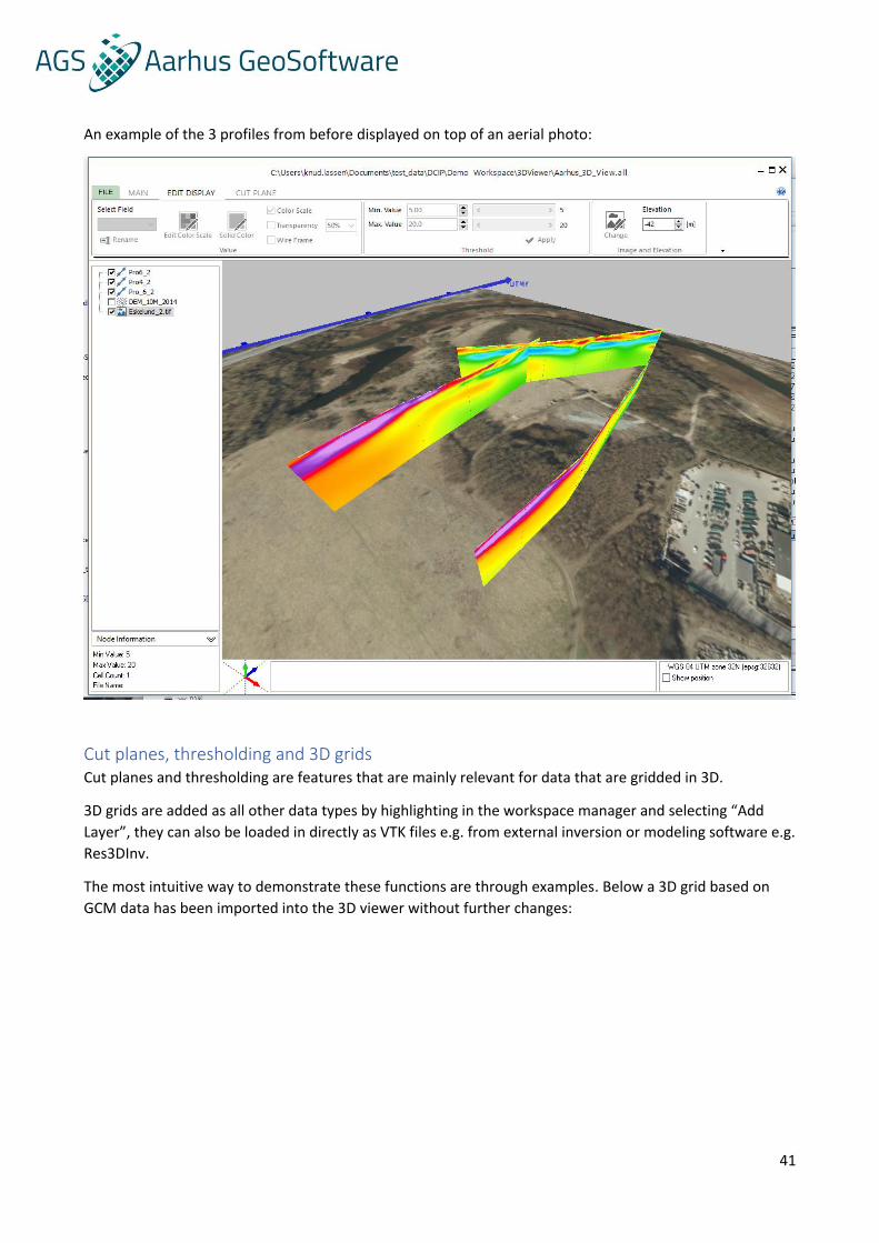
An example of the 3 profiles from before displayed on top of an aerial photo:
Cut planes, thresholding and 3D grids Cut planes and thresholding are features that are mainly relevant for data that are gridded in 3D.
3D grids are added as all other data types by highlighting in the workspace manager and selecting “Add
Layer”, they can also be loaded in directly as VTK files e.g. from external inversion or modeling software e.g.
Res3DInv.
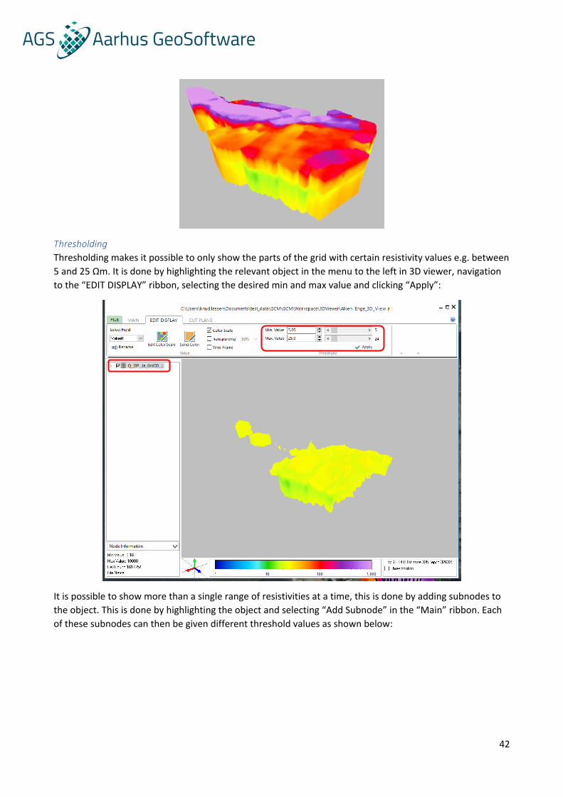
The most intuitive way to demonstrate these functions are through examples. Below a 3D grid based on
GCM data has been imported into the 3D viewer without further changes:
42
Thresholding
Thresholding makes it possible to only show the parts of the grid with certain resistivity values e.g. between
5 and 25 Ωm. It is done by highlighting the relevant object in the menu to the left in 3D viewer, navigation
to the “EDIT DISPLAY” ribbon, selecting the desired min and max value and clicking “Apply”:
It is possible to show more than a single range of resistivities at a time, this is done by adding subnodes to
the object. This is done by highlighting the object and selecting “Add Subnode” in the “Main” ribbon. Each
of these subnodes can then be given different threshold values as shown below:
43
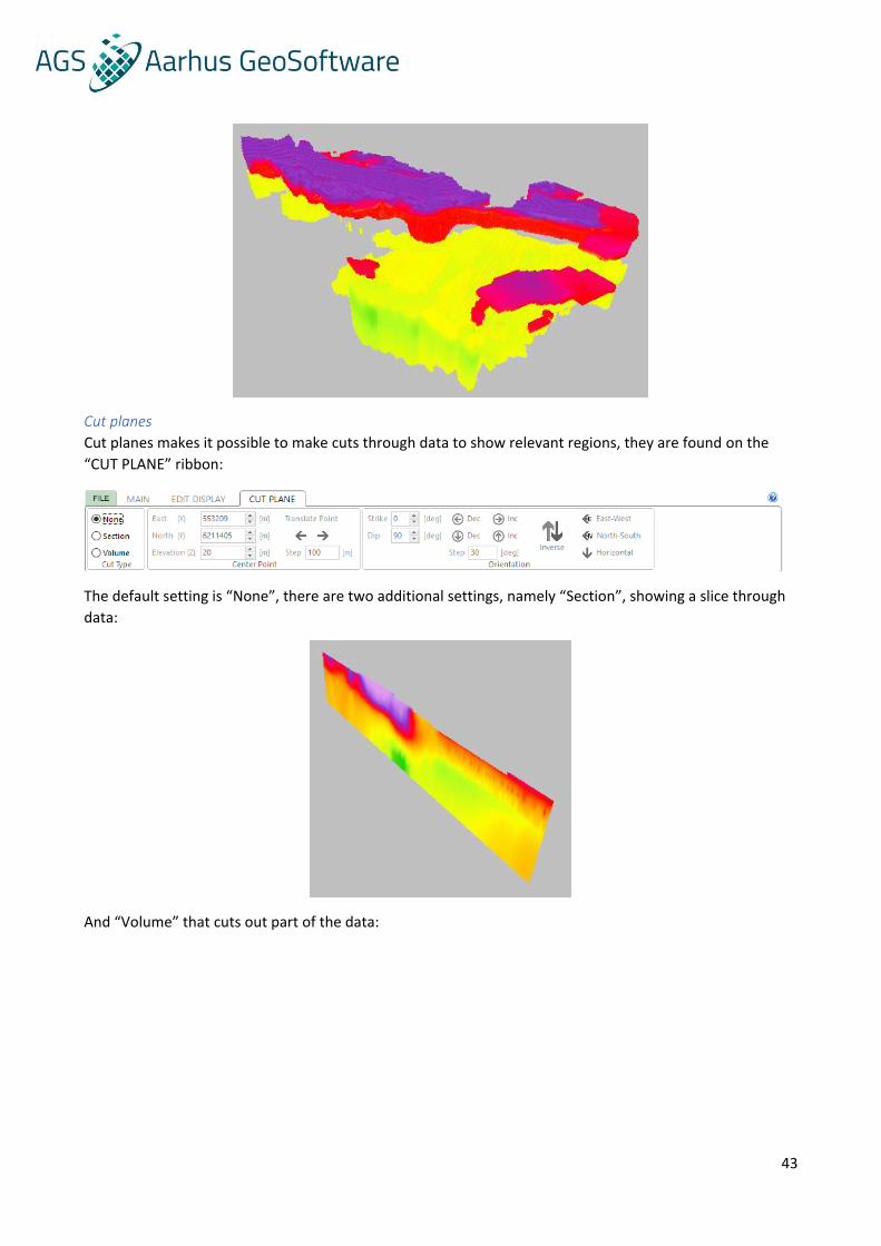
Cut planes
Cut planes makes it possible to make cuts through data to show relevant regions, they are found on the
“CUT PLANE” ribbon:
The default setting is “None”, there are two additional settings, namely “Section”, showing a slice through
data:
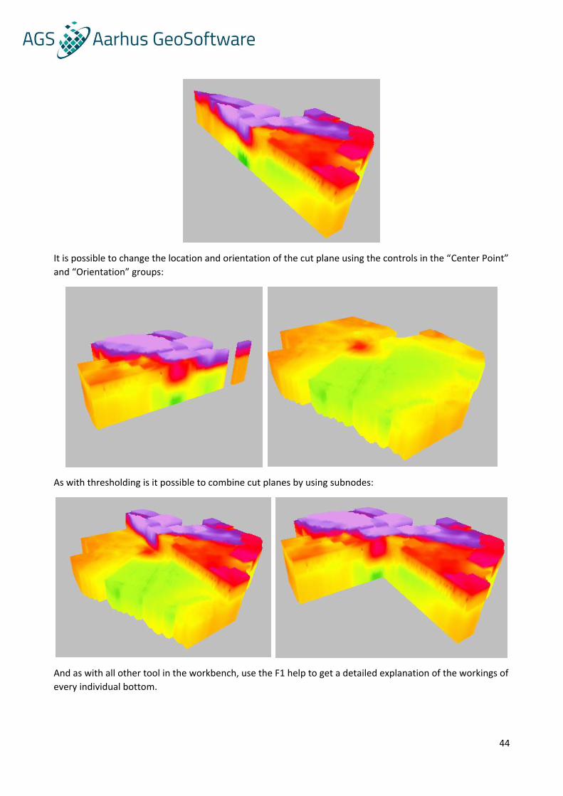
And “Volume” that cuts out part of the data:
44
It is possible to change the location and orientation of the cut plane using the controls in the “Center Point”
and “Orientation” groups:
As with thresholding is it possible to combine cut planes by using subnodes:
And as with all other tool in the workbench, use the F1 help to get a detailed explanation of the workings of
every individual bottom.

45
Export
The pictures created with the 3D viewer can be saved by pressing “save image” in the “main” ribbon or
copied directly to the clipboard by pressing “clipboard”. It is also possible to record the rotation of the 3D
view into a little movie (Only possible from ver. 5.8), this is done by pressing “Rec Start” and naming the
video file when prompted, all movements will be recorded until “Rec stop” is pressed.