Embed Size (px)
Citation preview
HAL Id: tel-01652884https://hal.archives-ouvertes.fr/tel-01652884v2
Submitted on 13 Mar 2018
HAL is a multi-disciplinary open accessarchive for the deposit and dissemination of sci-entific research documents, whether they are pub-lished or not. The documents may come fromteaching and research institutions in France orabroad, or from public or private research centers.
L’archive ouverte pluridisciplinaire HAL, estdestinée au dépôt et à la diffusion de documentsscientifiques de niveau recherche, publiés ou non,émanant des établissements d’enseignement et derecherche français ou étrangers, des laboratoirespublics ou privés.
Workflow variability modeling in microelectronicmanufacturing
Kean Dequeant
To cite this version:Kean Dequeant. Workflow variability modeling in microelectronic manufacturing. Business adminis-tration. Université Grenoble Alpes, 2017. English. �NNT : 2017GREAI042�. �tel-01652884v2�

THÈSE
Pour obtenir le grade de
DOCTEUR DE LA COMMUNAUTE UNIVERSITE GRENOBLE ALPES
Spécialité : Génie Industriel
Arrêté ministériel : 25 mai 2016
Présentée par
Kean DEQUEANT Thèse dirigée par Marie-Laure ESPINOUSE Et codirigée par Pierre LEMAIRE et Philippe VIALLETELLE, Expert en Science du Manufacturing chez STMicroelectronics préparée au sein du laboratoire des Sciences pour la conception, l’Optimisation et la Production (G-SCOP) dans l'École Doctorale Ingénierie - Matériaux, Mécanique, Environnement, Energétique, Procédés, Production (IMEP2)
Modélisation de la variabilité des flux de production en fabrication microélectronique Thèse soutenue publiquement le 9 novembre 2017, devant le jury composé de :
M. Alexandre DOLGUI Professeur à l’IMT Atlantique, président
Mme Alix MUNIER Professeur à l’UPMC, rapporteur
M. Claude YUGMA Professeur à l’EMSE, rapporteur
M. Emmanuel GOMEZ Manager Production chez STMicroelectronics, invité
M. Guillaume LEPELLETIER Expert en Science du Manufacturing chez STMicroelectronics, invité
M. Michel TOLLEANERE Professeur à Grenoble INP, invité Mme Marie-Laure ESPINOUSE Professeur à l’Université Grenoble Alpes, membre
M. Pierre LEMAIRE Maitre de conférences à Grenoble-INP, membre
M. Philippe VIALLETELLE, Expert en Science du Manufacturing chez STMicroelectronics, membre

2

3
If you go back a few hundred years, what we take for granted today would seem like magic: being
able to talk to people over great distances, to transmit images, flying, accessing vast amounts of data
like an oracle. These are all things that would have been considered magic a few hundred years ago.
-Elon Musk


5
Acknowledgements
Completing a PhD may sound to some like walking a lonely road for 3 years. It is, in fact, rather the
opposite. A PhD is an obstacle course, exciting and fulfilling, but also paved with problems, failures,
and uncertainties; and crossing the finish line is only possible thanks to all the people that are here to
give you a leg up along the way. I would like to thank all the people that helped me during the 3 years
of this PhD, who were there to share my excitement during my highs and to help me during my lows.
I would first like to thank my three tutors, Marie-Laure Espinouse, Pierre Lemaire, and Philippe
Vialletelle, for dedicating so much time and efforts to help me in this achievement. Most of all, it is their
constant support and their human qualities that allowed me to overcome the challenges of this PhD, and
for that I am infinitely thankful.
I would also like to thank all my colleagues from G-SCOP: the PhD students, the researchers, the
professors, as well as all the administrative staff who all form a great family with whom I shared some
wonderful moments. I am especially thankful to Michel Tolleanere, for his help in finding this PhD as
well as for his advices and wisdom which has brought me a lot.
I had a great experience at ST, and will keep many good memories from my time with my colleagues
and friends there. The Advanced Manufacturing Methods team was a great example of team working,
leadership, and friendship. To Emmanuel, Philippe, Guillaume, Renault, Soidri, Cédric, Laurence,
Bruno, Jérôme, Amélie, Alexandre, Quentin, Ahmed: thank you for everything.
Most importantly, nothing would have been possible without the support of the people the closest to
me in this world. To my friends, family, and to the love of my life, thank you for always being there for
me, for never letting me down, and for always pushing me forward in life.


7
Content
ACKNOWLEDGEMENTS ......................................................................................................... 5
CONTENT ......................................................................................................................... 7
GENERAL INTRODUCTION...................................................................................................... 9
I What is “variability”? .................................................................................. 11
1. THE IMPACT OF VARIABILITY ON MANUFACTURING ACTIVITIES ................................................ 13 1.A. Different acceptations of variability ................................................................................................ 14 1.B. STMicroelectronics: a case study on semiconductor manufacturing .............................................. 21
2. THE ANATOMY OF VARIABILITY: WHAT, WHERE AND HOW MUCH? .......................................... 25 2.A. Definitions of variability in the context of production flows ........................................................... 26 2.B. About measuring workflow variability ............................................................................................ 27 2.C. How NOT to measure workflow variability in complex systems ...................................................... 28 2.D. Proposed measures of local workflow variability ............................................................................ 31 2.E. Decomposing a manufacturing system into local process-clusters ................................................. 38 2.F. Workflow variability: a starting point for improving production management .............................. 47
3. THE ORIGIN OF WORKFLOW VARIABILITY: A LITERATURE REVIEW ............................................ 49 3.A. Scanning the literature of workflow variability ............................................................................... 50 3.B. Beyond the literature: insights on accounting for variability .......................................................... 56
II Integrating variability (in production management tools) .......................... 59
4. MAESTRO: INTEGRATING BACKGROUND VARIABILITY ........................................................... 61 4.A. Projection tools using cycle time models ......................................................................................... 62 4.B. Measuring the background consequences of variability ................................................................. 64 4.C. Dealing with the shift of background variability ............................................................................. 72 4.D. Integrating background variability: conclusion ............................................................................... 79
5. THE CONCURRENT WIP: A SOLUTION TO ANALYZE COMPLEX SYSTEMS ...................................... 81 5.A. The problem with simple models applied to complex (variable) systems ....................................... 82 5.B. A novel approach: the Concurrent WIP ........................................................................................... 83 5.C. Use case example: capacity analysis of semiconductor toolsets ..................................................... 87 5.D. Perspectives for the use of Concurrent WIP .................................................................................... 91
6. DEPENDENCY EFFECTS: IMPROVING THE KNOWLEDGE ON THE SOURCES OF VARIABILITY ................. 93 6.A. The need to understand the mechanisms of variability .................................................................. 94 6.B. An experiment framework for testing the variability potential of dependencies ............................ 95 6.C. Testing downtimes, arrivals, and process-times for variability induced by dependencies on industrial data ............................................................................................................................................ 101 6.D. Conclusion and perspectives.......................................................................................................... 106
III Towards variability reduction .................................................................. 109
7. A PLAN TO IDENTIFY VARIABILITY REDUCTION LEVERS (USING SIMULATION) .............................. 111 7.A. Master plan: study the past to change the future ......................................................................... 112 7.B. Improving knowledge on individual sources of variability ............................................................ 113 7.C. Modelling of dependencies............................................................................................................ 115 7.D. Improving the modelling of process-clusters with feedback loops ................................................ 117

8
7.E. Root cause analysis through simulation ........................................................................................ 123 7.F. Conclusion, perspectives and further research .............................................................................. 128
8. FURTHER PERSPECTIVES FOR VARIABILITY REDUCTION ......................................................... 131 8.A. Investigating variability on a global scale ..................................................................................... 132 8.B. Implementing variability reduction in a company ......................................................................... 136
GENERAL CONCLUSION...................................................................................................... 141
GLOSSARY ..................................................................................................................... 143
TABLE OF FIGURES ........................................................................................................... 147
TABLE OF TABLES ............................................................................................................. 149
REFERENCES ................................................................................................................... 151
SUMMARY..................................................................................................................... 156

9
General introduction
Moore’s law has been the lifeblood of semiconductor manufacturing strategies for the last 40 years.
The self-fulfilling prophecy made by the co-founder of Intel in 1965, stating that the number of
components per integrated circuit would double every two years, made transistors density the main
driver for competitiveness in the semiconductor industry for almost half a century. However, as
fundamental limits to components miniaturization are getting closer and closer (we are now reaching
gate sizes of 5 nm, around 10 atoms long), many actors are turning to a different competitive strategy,
advancing along the “More than Moore” axis. The More than Moore paradigm [1] consists in switching
from single architectures that can be used to perform any task to manufacturing specialized architectures
with higher performances for specific applications, and is driven by the special needs of smartwatches,
autonomous cars and more globally the rise of the “internet of things”. As this trend is focused on more
diversified products in lower quantities, it changes the rules of the game and sets delivery precision and
short delivery times as a new “sinews of war”.
It is however inherently difficult to reduce delivery times (referred to as cycle times in the industry)
and increase delivery precision in the particular manufacturing environment (of High Mix Low Volume
manufacturing systems) required to manufacture many different products in parallel in (relatively) small
quantities. The main reason to that is referred to as “variability”: “variability” translates the inevitable
fluctuations in the manufacturing flows which create uncontrolled and unpredictable “traffic-jams”.
Even though most companies and academics agree on the negative consequences of variability, little is
known about the essence of variability, the mechanisms involved, and how to effectively cope with it in
order to be more competitive.
This manuscript will address this issue of variability in complex manufacturing environment. The
research that we will present was conducted through a CIFRE PhD (an industrial PhD) between the G-
SCOP laboratory (Grenoble laboratory of Science for Conception, Optimization and Production) and
STMicroelectronics, a High Mix Low Volume semiconductor manufacturer with two key manufacturing
facilities (Crolles 200 and Crolles 300 fabs) located in Crolles, France.
The manuscript is divided in three main parts. The first part aims at explaining in depth what
“variability” really stands for, and is composed of chapters 1, 2, and 3. Chapter 1 gives an overview of
variability and shows that, even though the work is based on semiconductor manufacturing, it covers a
much larger spectrum as managing variability is a key ingredient in the development of Industry 4.0, a
growing standard for industries of the future. Chapter 2 then zeros-in on the main topic by introducing
the central notion of “workflow variability” and covering the more-than-meets-the-eye question of
measuring workflow variability in manufacturing systems. Chapter 3 then focuses on the root causes of
variability through an extended literature review, examples, and our experience in a real world
manufacturing system.
The second part of this manuscript is organized around the integration of variability in production
management tools, or in layman’s term: how to deal with workflow variability. To that extent, we first
show in chapter 4 how the projection/planification process of a company suffering high variability can
be improved by integrating the consequences of workflow variability on cycle time, thus increasing the
control on the system and countering the effects of workflow variability. We then discuss in chapter 5

10
how the current lack of proper measurement of the performances of process-clusters* (or toolsets*) is
holding back the development of tools and models to integrate further variability. To address this issue,
we introduce a new concept: the Concurrent WIP, along with associated tools and measures which allow
a proper measurement of process-clusters performances even in the presence of many complex sources
of variability. Chapter 6, our last chapter dedicated to the integration of variability, addresses underlying
mechanisms that create workflow variability. We show, based on industrial data, how dependencies in
the different events that occur in a manufacturing environment is a key to understanding workflow
variability.
Finally, part Three of this manuscript addresses perspectives of variability reduction. We show in
chapter 7 how we believe simulation tools fueled by real data can be used to identify actual levers to
reduce workflow variability, and we structure around this the several steps to start reducing workflow
variability on the short-term. The last chapter, chapter 8, organizes perspectives of variability reduction
on a much larger time scale. We show the potential of addressing global aspects of workflow variability,
and propose a flagship around which we articulate a framework (for both research and company
structure) to incrementally reduce workflow variability in a manufacturing environment over the next
10 years.
As this manuscript summarizes the work of a CIFRE PhD, it relies on both academic and industrial
work. As such, all the work in this manuscript was either published or oriented towards an industrial
application. The work from chapter 4 was implemented and industrialized to improve the WIP
projections at both STMicroelectronics Crolles fabs. Chapter 3 was presented at the 2016 Winter
Simulation Conference (WSC) [2], chapter 5 shows work presented at the 2016 International Conference
on Modeling, Optimization & Simulation (MOSIM) [3] and submitted to the journal of IEEE
Transactions on Automation, Science and Engineering (TASE), and chapter 6 covers works presented
at the 2017 International Conference on Industrial Engineering and Systems Management (IESM).
11
Part One
I What is “variability”?
“Variability” is a disturbing notion. In the context of manufacturing workflows*, it refers to a
phenomenon that affects the workflow and results in time loss and reduced delivery accuracy, but is far
from being properly understood.
This first part of this manuscript explains in depth what “variability” really is. We first explain
(chapter 1) what phenomenon “variability” translates and how this generates the negative consequences
one should be concerned about when it comes to manufacturing activities. Chapter 1 also explains what
type of manufacturing structure the research applies to and gives the specificities of the semiconductor
industry in which the research was conducted.
Chapter 2 then zeros-in on the main topic by introducing the notion of “workflow variability”: by
understanding that the variability is about the workflow, one can then focus on the proper way to
measure it. We explain in chapter 2 the difficulty of measuring workflow variability, the traps not to fall
into while trying to do so, and a proposed approach to allow this quantification of workflow variability.
We then explain how a local approach on studying workflow variability requires dividing the
manufacturing system into process-clusters and how we can rigorously split the system into what we
call “highly connected process-clusters”.
The last chapter of this part (chapter 3) focuses on the root causes of variability. Through an extended
literature review, examples and our experience in a real world manufacturing system, we give an
extensive list of the sources of variability which we classify into four categories (equipment specific,
product-induced, operational and structural). This work, which was published in the WSC conference
[2] and cited in a worldwide semiconductor Newsletter [4], also allows a better understanding of why
High Mix Low Volume (HMLV*) production is so prone to workflow variability compared to traditional
production lines.

13
Chapter 1
1. The impact of variability on
manufacturing activities
The term “variability” is used in the industry to refer to the phenomenon behind the congestions that
affect the Work-In-Progress (WIP*). More specifically, people put behind this word the notion that they
do not control these congestions as they seem to happen unexpectedly. This unpredictability is agreed
to have major consequences on the production as it makes companies lose time, money and delivery
accuracy. It seems, though, that not every manufacturing facility is affected the same way: High Mix
Low Volume production plants are reportedly much more affected by this “variability” and its negative
consequences.
This first chapter of this manuscript starts by giving an overview of this notion of “variability”, to
provide the reader with a basic understanding of what “variability” means in the context of workflow
management. We show the impact this variability has on flows in general and in the context of
manufacturing activities in particular. We explain the basic mechanism which makes variability create
more congestions and increase the cycle times, and why these cycle times matter when it comes to
manufacturing activities. We then transition to the more specific type of manufacturing [High Mix Low
Volume] where variability plays an even more central role as it is both present to a higher degree and
has a stronger impact on the ability to control the manufacturing system.
As this PhD was conducted in collaboration with STMicroelectronics (a High Mix Low Volume
semiconductor manufacturing company), this manuscript is centered on the semiconductor industry and
uses many examples with industrial data from the Crolles fab* of STMicroelectronics. Therefore, the
second part of this first chapter covers the specificities of High Mix Low Volume semiconductor
manufacturing all the while explaining why the research conducted here is applicable to any type of
manufacturing system and why we believe it is particularly crucial for the future of manufacturing.
Part One - What is “variability”?
14
1.A. Different acceptations of variability
1.A.1. Traffic jams and the problem of non-uniform flows
Traffic jams are (almost) everyone’s nightmare. Except if you are the CEO of a multinational
travelling by helicopter, or if you are lucky enough not to need a car in your life, you certainly
experienced traffic jams and the frustration that comes with the time loss it creates. If not in a car, you
certainly experienced queuing in a supermarket, waiting at a calling-center, or lining for security check
at the airport…
Though the context is different, the underlying phenomenon is the same in all cases, formally known
as “queuing”. The basic reason clients (cars, people, products…) queue is scarcity of resource: for a
given period of time, the resource available (road, cashier, call-center operator, security guard…) is
lower than what is needed to treat immediately all the clients that arrive in this period of time. This
situation is formally known as a “bottleneck” situation (as the same phenomenon explains why it takes
some time for a bottle tipped upside-down to empty) or an over-saturation.
The type of traffic jam (and therefore queuing or bottleneck) that is of interest here respects the
condition that on average (i.e. on the long term) the available resource is greater than the demand for
the resource (think of the previous cases: the road is empty at night, there are no more customers when
the supermarket closes, and security lines are empty at night, therefore on the long term the available
resource is greater than the demand). Necessarily, this implies that something is not constant in time
(otherwise the resource would always be greater than the demand). It is this inconsistency, either in the
clients’ arrivals or in the availability of the resources that generates the queuing. For instance, morning,
evening, or holiday traffic jams occur because at these periods of time, there are more cars fighting for
the same resource (the road). One (hypothetical) solution would be to oversize the resources to always
have more resource than demand. Obviously, in most cases, we choose not to do so as resources cost a
lot.
One could then choose to adjust the capacity to the demand. In supermarkets for instance, we know
that more cashiers are needed when people leave work as well as on Saturdays. However, on top of these
predictable variations comes a part of uncertainty and unpredictability in when and how long these
variations and non-uniformities might occur, and it seems that, as we are not able to predict them, we
are doomed to suffer their consequences, i.e. queue and wait…. This “variability” is the heart of the
problem that we study through this manuscript.
Manufacturing facilities are no exception to the rule: as the “traffic” of unfinished goods (that is, the
WIP) has to travel from and to different process-units*, non-uniformities in the flows of products and
the resources make some products request the same process-unit resource concurrently, which inevitably
results in unwanted waiting time. One consequence of this phenomenon is that it takes longer for each
product to travel through the entire manufacturing line (as each product has to do all its processing steps
and often wait behind others).
As this problematic is a major source of inefficiency, it has drawn attention and has been studied for
more than a century. A major approach to the problem comes from mathematics, as the science of
describing the interactions between servers and clients in a stochastic environment, and known as
queuing theory.
Chapter 1 - The impact of variability on manufacturing activities
15
1.A.2. Queuing theory: early works on understanding variability
Erlang [5] was the first (1909) to mathematically describe the stochasticity in clients/servers systems
in what is now called “queueing theory”. The first model assumed markovian arrivals and markovian
services (or process-times*) and a unique server, and is formally known as an M/M/1 queue (in
Kendall’s notation [6]). In 1930, Pollaczek [7] extended the model to general service laws (including
for instance normal distributions) to address M/G/1 queues. This formula is however restricted to a
unique server. Since then, many new queuing models have been proposed. The work of Whitt ([8]–[11])
being for instance famous for proposing G/G/m models (general arrivals and processes with multiple
servers) and therefore allowing to study more general systems.
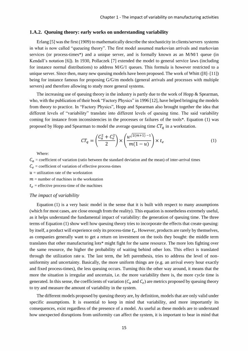
The increasing use of queuing theory in the industry is partly due to the work of Hopp & Spearman,
who, with the publication of their book “Factory Physics” in 1996 [12], have helped bringing the models
from theory to practice. In “Factory Physics”, Hopp and Spearman also brought together the idea that
different levels of “variability” translate into different levels of queuing time. The said variability
coming for instance from inconsistencies in the processes or failures of the tools*. Equation (1) was
proposed by Hopp and Spearman to model the average queuing time 𝐶𝑇𝑞 in a workstation.
𝐶𝑇𝑞 = (𝐶𝑎
2 + 𝐶𝑒2
2) × (
𝑢√2(𝑚+1) −1
𝑚(1 − 𝑢)) × 𝑡𝑒 (1)
Where:
𝐶𝑎 = coefficient of variation (ratio between the standard deviation and the mean) of inter-arrival times
𝐶𝑒 = coefficient of variation of effective process-times
𝑢 = utilization rate of the workstation
𝑚 = number of machines in the workstation
𝑡𝑒 = effective process-time of the machines
The impact of variability
Equation (1) is a very basic model in the sense that it is built with respect to many assumptions
(which for most cases, are close enough from the reality). This equation is nonetheless extremely useful,
as it helps understand the fundamental impact of variability: the generation of queuing time. The three
terms of Equation (1) show well how queuing theory tries to incorporate the effects that create queuing:
by itself, a product will experience only its process-time 𝑡𝑒. However, products are rarely by themselves,
as companies generally want to get a return on investment on the tools they bought: the middle term
translates that other manufacturing lots* might fight for the same resource. The more lots fighting over
the same resource, the higher the probability of waiting behind other lots. This effect is translated
through the utilization rate 𝑢. The last term, the left parenthesis, tries to address the level of non-
uniformity and uncertainty. Basically, the more uniform things are (e.g. an arrival every hour exactly
and fixed process-times), the less queuing occurs. Turning this the other way around, it means that the
more the situation is irregular and uncertain, i.e. the more variability there is, the more cycle time is
generated. In this sense, the coefficients of variation (𝐶𝑎 and 𝐶𝑒
) are metrics proposed by queuing theory
to try and measure the amount of variability in the system.
The different models proposed by queuing theory are, by definition, models that are only valid under
specific assumptions. It is essential to keep in mind that variability, and more importantly its
consequences, exist regardless of the presence of a model. As useful as these models are to understand
how unexpected disruptions from uniformity can affect the system, it is important to bear in mind that

Part One - What is “variability”?
16
they might only partially describe how “variability” is generated, what it actually is, and what
consequences it has on entire systems.
1.A.3. Manufacturing systems: where cycle times matter
In simple, mono-product assembly lines, increased cycle times may not seem to be a huge problem.
Indeed, for this type of production, the essential aspect seems to be the ability to meet the throughput
rate, whether the cycle times are short or long: if we need to deliver 100 products a week to our clients,
do we really care how long each product takes to finish, as long as we deliver 100 products a week?
Yes. Yes we do care. Little’s law [13] tells us that increased cycle times necessarily come with increased
Work-In-Progress (the unfinished goods that require further processes to be delivered). This means that,
for any manufacturing facility, increased cycle times directly and proportionally translate into increased
inventory of unfinished goods, i.e. more immobilization of assets and more cash required to run the
business (each unfinished good required money to produce it, but has not yet brought money back as it
has not been sold yet). Higher cycle times also translate into more latency in the detection of problems
and non-conformities: if quality inspection is performed on finished products, a higher cycle time means
that more products can undergo a defective process before the detection of the first out-of-spec product
and therefore more products are at risk of being scraped (thrown away). The impact and cost of cycle
time is the reason reducing cycle times and keeping low WIP inventory is one of the central objectives
of Lean Manufacturing [14].
As variability is the main driver of queuing time (and therefore cycle time), keeping a low variability
in the system is a fundamental key to successful manufacturing companies.
1.A.4. High Mix Low Volume: the European model
Survival of the fittest
Modern manufacturing is commonly agreed to have started with Ford and the production line of the
first mass-produced car: the Ford Model T. The standardization of the production and the partial
automatization of the assembly line allowed for economies of scale: the inverse relationship between
the number of units produced and the cost of each unit. In layman’s term, the more you make, the less
it costs. For instance, economies of scale is the reason Tesla is building its Giga-Factories: Tesla wishes
to drastically reduce the cost of its batteries and cars by pushing the concept to an unprecedented level;
mutualizing the resources, tools, machinery, and engineering to the limit. What economies of scale
actually translate is that, like everything, manufacturing obeys the simple law of evolution: survival of
the fittest. Survival of the fittest means adapting the best to the environment (a concept more formally
known as “Porter’s diamond” [15] in economics, see Figure 1). Economies of scale is a good strategy
to adapt. However, the equally important word in “adapting to the environment” is “environment”. The
economic environment, as the natural environment, greatly differs from one region to another. Europe,
for instance, does not have the same volumes of domestic demand as the US and Asia. These internal
markets are essential for the initial phase of a company as they allow small shipping costs, good
knowledge of the regulations, quite often local government helps… which all help to a rapid production
ramp-up and a relatively short payback period on massive investments. The volumes of most European
manufacturing companies are therefore bounded by their environment, which also includes more strict
regulations (meaning less flexibility for the companies) and older existing infrastructures which need to
be built upon (instead of starting from scratch).

Chapter 1 - The impact of variability on manufacturing activities
17
Europe’s environment is different than US and Asia environment, and in this setting, Europe cannot
compete in the Low Mix High Volume league (producing few products in very large volumes).
However, Europe’s environment is different in other ways, which can bring competitive advantages
from other axis. One main aspect of Europe is that the population is extremely heterogeneous: there are
many different countries, cultures, traditions, backgrounds, religions, etc. This diversity means that there
is a high demand in Europe for different products: the demand is not in slight modifications such as the
color or an extra option, but in different products from the core. Contrary to customization, these
differences are too big to allow different products to follow the same assembly line: the order and nature
of the processing steps are different. In this environment, the fittest companies, the best suited for
survival, are the ones that are able to achieve economies of scale by simultaneously producing many
different products: this is the realm of High Mix Low Volume production.
Figure 1: Porter’s diamond [15], the environment of a company
Europe’s manufacturing has been at the back of the pack the last couple of decades. The reason is
not that US and Asia manufacturing are better suited, it is that they were better suited to their
environment than Europe’s manufacturing was to its environment. Indeed, producing in High Mix Low
Volume adds a lot of complexity to the manufacturing process. Up to recently, the information
management and technology required to tell each machine and each worker what manufacturing step to
process on what product at what time was too much to handle efficiently, and the product-mix* and
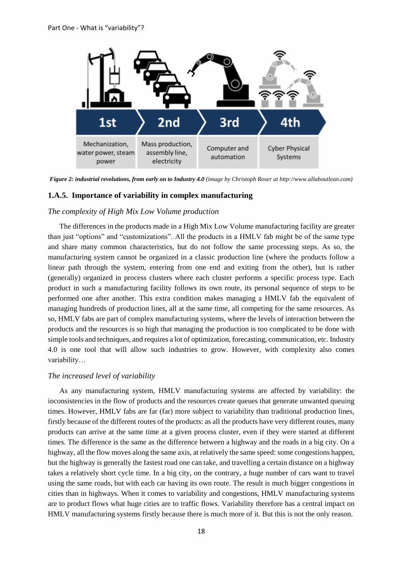
volumes had to stay relatively small to manage such systems. However, today, the rise of “Industry 4.0”
- a growing standard of communication and information management in complex automatized
manufacturing environments, see Figure 2 and [16]- is the mutation required in the European industry
to evolve into the most fitted type to its environment: High Mix Low Volume production. This type of
production allows competing relatively well along the cost side (with economies of scale), all the while
taking leadership in product diversification. The potential of such industries in the coming decades is
huge, as the pace of change in the demand is increasing more rapidly than ever with the democratization
of internet and new trends such as the “internet of things”.
Part One - What is “variability”?
18
Figure 2: industrial revolutions, from early on to Industry 4.0 (image by Christoph Roser at http://www.allaboutlean.com)
1.A.5. Importance of variability in complex manufacturing
The complexity of High Mix Low Volume production
The differences in the products made in a High Mix Low Volume manufacturing facility are greater
than just “options” and “customizations”. All the products in a HMLV fab might be of the same type
and share many common characteristics, but do not follow the same processing steps. As so, the
manufacturing system cannot be organized in a classic production line (where the products follow a
linear path through the system, entering from one end and exiting from the other), but is rather
(generally) organized in process clusters where each cluster performs a specific process type. Each
product in such a manufacturing facility follows its own route, its personal sequence of steps to be
performed one after another. This extra condition makes managing a HMLV fab the equivalent of
managing hundreds of production lines, all at the same time, all competing for the same resources. As
so, HMLV fabs are part of complex manufacturing systems, where the levels of interaction between the
products and the resources is so high that managing the production is too complicated to be done with
simple tools and techniques, and requires a lot of optimization, forecasting, communication, etc. Industry
4.0 is one tool that will allow such industries to grow. However, with complexity also comes
variability…
The increased level of variability
As any manufacturing system, HMLV manufacturing systems are affected by variability: the
inconsistencies in the flow of products and the resources create queues that generate unwanted queuing
times. However, HMLV fabs are far (far) more subject to variability than traditional production lines,
firstly because of the different routes of the products: as all the products have very different routes, many
products can arrive at the same time at a given process cluster, even if they were started at different
times. The difference is the same as the difference between a highway and the roads in a big city. On a
highway, all the flow moves along the same axis, at relatively the same speed: some congestions happen,
but the highway is generally the fastest road one can take, and travelling a certain distance on a highway
takes a relatively short cycle time. In a big city, on the contrary, a huge number of cars want to travel
using the same roads, but with each car having its own route. The result is much bigger congestions in
cities than in highways. When it comes to variability and congestions, HMLV manufacturing systems
are to product flows what huge cities are to traffic flows. Variability therefore has a central impact on
HMLV manufacturing systems firstly because there is much more of it. But this is not the only reason.

Chapter 1 - The impact of variability on manufacturing activities
19
The central impact of variability
The impact variability has on classical production lines remains true on HMLV manufacturing
systems: as variability affects the flow of products through the inconsistencies in the resources, the cycle
times are increased. Another reason why variability is much more important in HMLV systems than in
classical production lines is that cycle time itself is a much more critical aspect. We previously
mentioned the impact of cycle time on increased WIP (i.e. immobilized assets) and yield* (the
proportion of products started that make it to the selling point, the rest being thrown away). On top of
this, cycle time plays a huge role in HMLV production because of competitiveness. Indeed, as the
volumes for each product are low and the markets fast changing, delivery time is a key performance that
allows gaining new markets. The smaller the delivery times are, the more diverse and small the markets
addressed can be.
Cycle time is such a central aspect in many manufacturing areas that practitioners regularly use
special graphs describing the relation between cycle time and utilization: so-called “operating curves”
[17] (or “cycle time throughput curves”). These curves play a central aspect in understanding variability,
as they are used in a large number of papers (e.g., see [18]–[29]) to describe the impact of variability.
These curves, as shown in Figure 3.A, represent the normalized cycle time (also called Xfactor* [30],
i.e. the ratio between the cycle time and the raw-processing-time) versus the utilization rate of the tools
for a given toolset.
Figure 3: operating curves showing different levels of variability (A) and the link to capacity loss (B)
Understandably, the tools cannot be used more than 100% of the time, which bounds the maximum
utilization rate to 100%. Over 100%, lots would “infinitely” accumulate, thus creating “infinite” cycle
times. Therefore, for any toolset (i.e. queuing system), the queuing time starts at 0 (corresponding to an
Xfactor of 1) at a utilization rate of 0, and increases to infinity when approaching 100%. The operating
curves are the description of what happens in the middle, which actually translates the level of variability
at this toolset. In accordance with our previous description of the impact of variability, Figure 3.A shows
different curves for different levels of variability, and shows that an increase in variability generates an
increase in cycle time. The operating curves always show cycle time in relative manners using the
Xfactor ratio. Indeed, in real-world situations, what is important is not how long it takes to manufacture
products but rather if this time translates a good performance. For instance, if it takes two different
products respectively 50 days and 65 days of cycle time to be manufactured, can it be said that one
product translated better performances than the other? This question cannot be answered without
Part One - What is “variability”?
20
knowing the raw-processing-time. If we know, however, that the two previous products require
respectively 10 days and 13 days of raw-processing-time, we can then compute an Xfactor of 5 for both
products, and see that they actually had equal performances in terms of cycle time.
On top of the cycle time, another less obvious impact of variability is the capacity loss it generates.
We usually think of capacity loss as tools inefficiencies. Variability creates another kind of capacity loss
which is actually a strategic capacity loss. The link between capacity loss and variability arises from the
desire of companies to both maximize the utilization of their assets (in order to minimize the costs) and
keep an acceptable cycle time (to have fast delivery times and access more markets). As Figure 3.B
shows, the constraint on cycle time generally translates in a maximum allowed Xfactor. Because of the
link between cycle time and utilization depicted by the operating curves, setting a maximum allowed
Xfactor actually translates in setting a maximum allowed capacity utilization. However, setting a
maximum utilization rate means choosing not to fully use the tools. In practice, this choice translates by
not accepting all orders of clients as to not load the system passed the critical utilization level. Note that,
as Figure 3.A indicates, for a given Xfactor, a lower variability equals a higher utilization rate. Therefore,
lowering variability in a manufacturing system that has a constraint on cycle time (such as HMLV) can
significantly increase the resources effectively available and therefore increase the capacity of the entire
system without adding any resource. In a competitive world where margins are of only a few percent,
managing variability is a lever with a huge potential.
In addition to cycle time and capacity loss, another impact of variability arises when it comes to
HMLV production: tractability. Tractability is the ability to control the system and to be able to make
accurate forecasts about the future of the system (in particular about the flows of products in the system).
Tractability is of upmost importance in HMLV, because, again, of the markets addressed. Indeed, not
all products take the same time to be manufactured (as not all products have the same number of steps
or follow the same routes). Concurrently, different clients have different expectations in terms of cycle
times and delivery dates. In such setting, it is essential to know how long each product will take to finish
in the current manufacturing setting, and to be able to act on the system to speed up some of the products
and slow down some other ones to maximize the utilization of the resources while respecting all the
commitments to the clients. As variability creates unexpected and uncontrolled queuing times at the
different process clusters of the manufacturing systems, variability decreases the tractability of HMLV
manufacturing systems. Managing variability in HMLV manufacturing systems is therefore an
extremely central aspect of managing the system, as it is both much higher than in traditional systems
and much more (negatively) impactful.
1.A.6. The confusing aspects of variability
A manufacturing system is a global system. It comprises of different resources, operators, flows,
etc. Matters of cycle time, capacity loss, and decrease in tractability also take their importance when we
consider the entire manufacturing system. However, we first described variability through queuing
equations, which are models describing process clusters, not manufacturing systems. Therefore, we can
already see that there are different aspects to variability, different scales at which variability appears. To
this first mind-boggling aspect adds the problem of the definition of “variability”. As we mentioned the
term “variability” several times already and it is the central aspect of this manuscript, careful readers
would have noticed that we have not yet given any definition of the word. Through our description, we
mainly used the word variability in accordance to the definition of Oxford dictionaries: the “Lack of
consistency or fixed pattern; liability to vary or change”. However, the word usually describes another
quantity, phenomenon or unit: we can talk about “a great deal of variability in quality”, “seasonal

Chapter 1 - The impact of variability on manufacturing activities
21
variability in water levels”, etc. When it comes to manufacturing systems and workflows, the literature
is generally unclear on what variability qualifies. So far, we have seen that variability is a “lack of
consistency or fixed pattern; a liability to vary or change” that affects the flows of products, and is also
connected to the resources that treat these products. However, up to this part of the manuscript, the
question “variability of what?” does not have a clear answer.
Before clarifying the above points in the next chapter, we will now introduce the case study around
which the work of this PhD was conducted. Indeed, this PhD had the particularity to be a collaboration
between a research laboratory (G-SCOP) and a company (STMicroelectronics) through a type of
contract known as a CIFRE thesis. In this setting, the work was conducted with a general scope, however
using examples, data and vocabulary specific to the semiconductor industry.
1.B. STMicroelectronics: a case study on semiconductor manufacturing
1.B.1. An industrial PhD at STMicroelectronics
STMicroelectronics
STMicroelectronics is a company that develops, produces and commercializes microchips for
electronic systems. The company generated a revenue of 7 billion euros in 2016 and is settled in a dozen
countries in the world with 12 production sites and 39 conception sites. ST (the short name for
STMicroelectronics) was created in 1987 from the fusion of SGS Microeletronica and Thomson
Semiconducteurs and produces microchips for a wide range of applications that address 5 main markets
that are Microcontrollers, Automotive, MEMS & Sensors, Application Processors & Digital Consumer,
and Smart Power (Figure 4).
Figure 4: the main markets of STMicroelectronics
Semiconductor manufacturing is generally separated into two main steps which are referred to as
the front-end and the back-end activities. The front-end takes raw silicon substrate (wafers*) and
manufactures the transistors and the connections to create on the wafers the core elements of the
microchips. The back-end then receives these processed wafers, performs functional tests on the
microchips that are engraved in the wafers, and then cuts the microchips from the wafers and packages
them into single microchips that can be used on a motherboard or as part of an integrated product (Figure
5 shows microchips on wafers and after being packages). The front-end activity is by far the most
complicated and most expensive part of the process and is where most of the added-value is generated.

Part One - What is “variability”?
22
Figure 5: microchips engraved in wafers of different sizes are packages individually to be used in consumer products
Crolles manufacturing site, France
The site of Crolles was built in 1992 not long after the creation of the company. It is now a strategic
site that employs more than 4000 people and contributes to about a quarter of the company’s revenue.
The site of Crolles is composed of two fabs, a 200mm and a 300mm fab (referring to the diameter of the
wafers). The 300mm fab being the most recent one, it supports technologies that can engrave down to
10nm. At such small scales, the presence of dust or particles is extremely problematic, as it would create
(comparatively) huge misalignments it the different layers of materials that are deposited on the wafers.
The entire process therefore takes place in a clean room with cleanliness requirements one thousand
times greater than that of an operating room. This requires the entire architecture of the building to be
thought for this specific purpose. Several floors of filtering and air treatment therefore surround the
clean room and keep the air clean by injecting a laminar flow of air as to continuously expel in the floor
any particle created inside the room (Figure 6).
Figure 6: the laminar flow of a clean room
The transportation of the lots in the 300mm fab is fully automatized and run by the Automated
Material Handling System (AMHS), which is primarily composed of suspended robots travelling 35
km/h. As so, transportation times are generally negligible compared to queueing and process-times
inside the fab.
Objectives
As STMicroelectronics Crolles is a HMLV fab, it is subject to the issues we explained earlier: ST
wants to improve the tractability of its manufacturing system in order to enhance the delivery precision
for both a better clients’ satisfaction and an optimization of the resource utilizations. As the growing
segments of semiconductor markets are along “internet of things” and custom-made microchips, it is
also important for the company to further improve its cycle time as to secure the future markets and
become a leader early on. As this PhD is an “industrial PhD” (with a CIFRE contract), the research will
be targeted in directions that will allow the company to achieve its objectives in the near future. As this
PhD is focused on variability, the objectives of the research are to allow a better tractability of the system

Chapter 1 - The impact of variability on manufacturing activities
23
through better knowledge on variability, a better integration of variability in the production management
tools of the company, as well as building up structured knowledge on variability in a way that will allow
the company to reduce the variability and thus the negative impacts it has on the manufacturing system.
As several attempts to reduce variability have had questionable results, it is important to first take a step
back and ask the important question of what variability really is, with all the ramifications this rather
large question implies. This will help us understand what can be done straight away, what needs
complimentary knowledge and information to advance in the right direction, and what this direction
should be.
1.B.2. Characteristics of a High Mix Low Volume semiconductor manufacturing facility
Traditional production or assembly lines are usually organized to build products starting from raw
materials or components, progressively transforming or assembling them in order to deliver “end
products” or “finished goods”. Such factories manage a linear flow of products going all in one direction
from the beginning of the line to the end of the line. Regardless of whether process steps are performed
by operators or machines, process-times are subject to inconsistencies, machines are subject to
breakdowns, and operators and secondary resources are sometimes unavailable.
Semiconductor fabs are, like other industries, subject to the above mentioned “disturbances”. Their
main characteristic however, justifying the label of “complex environment”, is the reentrancy* of their
process flows. Microchips are produced by stacking tens of different layers of metals, insulators and
semiconductor materials on silicon substrates (called wafers). The similarities of layers, added to the
extreme machine costs, lead the same groups of machines (toolsets) to process different layers. Hence
products are processed several times by the same machines over the course of their hundreds of process
steps. Dedicating machines to steps is only (partially) possible in very large facilities (such as memory
fabs) where thousands of tools are generally producing one or two different products; these factories
operate in what is generally referred to as HVLM: High Volume Low Mix manufacturing.
The second characteristic of semiconductor manufacturing is that it involves different types of
physical processes that require different types of machines (see [31]). Batching machines, such as
deposition or diffusion furnaces for example, will process products in batches of different minimum and
maximum sizes according to the specific recipe* and process step. Other machines, such as cluster tools,
consist of process chambers or modules sharing the same robotics. Depending on the products being
processed at the same time, resource conflicts may appear within the tool, rendering process-times even
more inconsistent. Many other characteristics may also be cited here as semiconductor manufacturing
is above all a matter of technology and then only a matter of efficiency. A very good example is that
most semiconductor vendors still propose “lots of 25 wafers” as manufacturing units, whereas the move
to larger wafer sizes should already have challenged this paradigm.
A third characteristic of semiconductor fabs is the business model they use. While High Volume
Low Mix units usually produce in the range of 3 to 4 different products at the same time over one or
two different technology generations, High Mix fabs propose a wide variety of products to their
customers over several technology nodes. A difficulty in this case is that specific process steps may only
be required by very few products. Therefore, only 1 or 2 tools may be used to process a given group of
steps and toolsets in general need to be highly flexible (In the sense that each tool can have a unique but
changeable set of steps it is qualified on). Moreover, qualifying a “technology level” on a tool requires
time (as functional tests can only be performed on finished products) and money (as “testing wafers”
cannot be sold). Therefore, not all tools of a given toolset will be qualified on all the operations
associated to this toolset, thus adding heterogeneity of tools to the heterogeneity of products. High Mix
Part One - What is “variability”?
24
fabs, as they address a wide range of customers and products, generally follow a make-to-order policy.
Given the range of products, stocks cannot satisfy demands and lots are therefore started on demand
with different requirements in terms of delivery times. Production control techniques and rules are then
introduced to manage different levels of priorities* necessary to achieve the individual required speeds.
1.B.3. A targeted study for a generic application
Microelectronic manufacturing is a $300 billion state-of-the-art industry. The huge amount of
money involved in this industry, alongside the standardization that happened in the early 2000’s with
the development of the 300mm fabs and the continuous growth and pressure for innovations and
improvements created a perfect environment for research. In the few decades of existence, the research
field of semiconductor manufacturing has developed a common language and common standards for the
description of the different elements that compose a semiconductor manufacturing system. Moreover,
as the volumes are so enormous, there has been and will continue to be a continuous flow of research in
this field. Therefore, this PhD mostly restricted the research to semiconductor manufacturing.
Semiconductor manufacturing has one of the most complex environment in the world. Indeed, as
the making of a microchip involves an extreme wide range of physics (electronics, optical, materials,
signal processing, chemistry, dealing with gases and extreme temperatures…), the machines, processes,
and “machine logistics” in a semiconductor fab are extremely heterogeneous. However, other industries,
such as photonics [32] or more “traditional” industries [16] are also subject to high levels of complexity
and variability and face the same challenges as the semiconductor industry. Moreover, as “he who can
do more can do less”, the solutions to managing variability in HMLV semiconductor fabs will be
applicable, if not to all, to most other HMLV industries.
Chapter 2 - The anatomy of variability: what, where and how much?
25
Chapter 2
2. The anatomy of variability:
what, where and how much?
Chapter 1 introduced the notion of variability affecting workflow in manufacturing environments
through general examples and existing work in queuing theory. However, this notion of “variability”
remained fuzzy: if the consequences and importance are rather clear, the question of what variability is
has not been answered yet.
The objective of chapter 2 is therefore to provide the knowledge and the tools to get a deep
understanding of what variability really is and how it can be measured in a manufacturing system. First,
we will focus on the description of variability, providing definitions for the “intrinsic variability of a
manufacturing system” and most importantly for the central notion of “workflow variability”. The
notion of workflow variability will be the central aspect of this chapter as it allows putting all the pieces
of the puzzle together. We will explain in section 2.B how we can separate a manufacturing system into
different process-clusters in order to allow a measure of workflow variability. Most importantly, we will
discuss on how to make the measure: we will cover different possibilities that would seem intuitive and
good options at first sight but would actually fail to provide a correct measure because of the complexity
of the manufacturing environment. We will then propose a method that overpasses these challenges and
that allows measuring where and how much workflow variability there is in any given manufacturing
system.

Part One - What is “variability”?
26
2.A. Definitions of variability in the context of production flows
The link between variability (as described in chapter 1) and cycle time makes no doubt and is
understood by all practitioners in the field. However, the word variability itself makes most authors
uncomfortable as what lies behind remains fuzzy. At the toolset level, several authors have attempted to
attach variability to something: Hopp & Spearman [12] talked about the “variability of effective process-
time” and the “variability of inter-arrival times” and were followed by many other authors ([20], [33]–
[36]). However, these same authors also use the word variability on itself for instance when explaining
that “semiconductor industry should aim at reducing variability to provide low cycle times” [37].
Moreover, many authors make it clear that they do not talk about “arrivals variability” nor “effective
process-time variability” as they affect the word variability to the manufacturing system, such as [25]
who explain that “reducing the inherent variability of a manufacturing system improves the overall
system performance“. Even at the toolset level, Schoemig [25] talks about “the variability introduced
into a queuing system” as something different than “arrivals variability” and “effective process-time
variability”.
In order to structure our research on variability, we need solid bases to build upon. For this purpose,
we will clarify in this section what carries variability. This will have important implications for the
understanding of the problem, the way we can measure it, and throughout this manuscript, how we can
deal will it.
2.A.1. Workflow variability: the proper name for the proper consequences
Something carries variability. Something has a “Lack of consistency or fixed pattern, a liability to
vary or change”, and the fact that this something has variability is directly linked to increased cycle
times, decreased tractability, and capacity loss (as explained in chapter 1). From queuing theory and the
literature, we know that both the arrivals variability and the effective process-time variability participate
(under specific conditions) to the increase in the variability of this something. We also know that
increased variability of this something increases the variability of the manufacturing system.
If we visualize a manufacturing system as a river (or a sea), where the level of the water at each
position represents the amount of WIP at each toolset of the manufacturing system, a manufacturing
system with a low variability will be a calm stream (or a calm sea), with only small fluctuation then and
now. On the other hand, a manufacturing system with a high variability would be a mountain river
during a rainstorm (or a sea in rough weather), creating at all time huge variations in the level of the
water. From this example, we can understand that it is actually on the difference of levels of WIP in
time (the variations in the levels of water) that variability manifests itself. Therefore, in a manufacturing
system, the something is the workflow.
Thus, the variability that practitioners, operators, and academics are referring to, the one we are
concerned about is actually the workflow variability. At the toolset level, the incoming workflow can
already be variable because of the combined actions of all of the upstream toolsets, but the toolset can
modify the workflow variability either increasing it when suffering high capacity variations (which is
usually the case), or decreasing it (locally) if it is able to synchronize with the incoming waves of
workflow variability. In front of the toolset, the workflow variability locally manifests through varying
levels of WIP. Downstream, the toolset sends the workflow to one or many other toolsets, which receive
WIP also from one or many other toolsets. The workflow variability is the result of all these interactions.
In a complex manufacturing system with high reentrancy, WIP waves can leave simultaneously from
Chapter 2 - The anatomy of variability: what, where and how much?
27
different toolsets and concurrently arrive at a given toolset, smashing at once on the capacity of that
toolset and locally creating huge WIP levels.
More formally, we can define workflow variability as the liability of workflow to vary or change
and to lack consistency or fixed pattern. On the smallest possible level, these variations occur when
some lots are waiting, i.e. when there are no resource (e.g. no tool) available to perform the required
task on the lots (i.e. when there is over-saturation). Workflow variability therefore translates the
tendency to generate these over-saturations, and as earlier works have shown, variability in the arriving
flow as well as variability in the capacity of the toolset both participate to workflow variability as they
both participate in a wider range of saturations and therefore in more over-saturations. For ease of use,
we will sometimes refer about workflow variability simply as “variability” such as when mentioning
that there is “low variability” or “high variability”, but we should always keep in mind that from now
on, variability refers to workflow variability.
2.A.2. The intrinsic variability of a manufacturing system
Workflow variability is what happens locally in a system, it is the ripples on a pond, the waves in
the ocean. Many authors however talk about the variability “of a manufacturing system”. By doing so,
they are translating the overall behavior of the system: if the variability of the manufacturing system is
high, it has high overall cycle times and degraded performances. In our previous analogy, this would
translate the state of the river: whether it is calm, rough, or wild.
In accordance with this, we can define the intrinsic variability of a manufacturing system as its
corrupting tendency to generate uncontrolled unevenness both in its flows and in the capacities of its
manufacturing resources, resulting in efficiency losses, i.e. non-productive waiting times. In other
words, the intrinsic variability of a manufacturing system is its tendency to generate workflow
variability.
2.B. About measuring workflow variability
2.B.1. The difficulty of measuring workflow variability
Workflow variability as we defined it is a phenomenon, not a measure. As so, it has the advantage
to stay general and to keep the focus on the implications (increased cycle time, decreased tractability,
and capacity loss). The downside is that the definition remains scientifically and mathematically vague.
Actually, directly measuring workflow variability would be extremely difficult because of the
complexity it would involve. First, the notion of variability does not have a defined mathematical
description. Some measures exist, such as the standard deviation, the inter-quartile range, etc. but these
have definitions of their own and, even though they measure some aspects of variability, they do not
define it. Second, a workflow is a movement of products. As so, there are at least three quantities
describing a workflow: an amount (of products, lots, wafers…), a distance (or notions close to a distance
such as going from step A to step B), and a time (e.g. time required to go from step A to step B). Directly
measuring workflow variability would mean measuring the variability of these three dimensions. In a
complex system, the different possible combinations of distances and time intervals required to give a
full description of workflow variability are enormous and would therefore require extremely complex
mathematics. Therefore, even though workflow variability might be possible to describe
mathematically, we will keep workflow variability as a phenomenon, as the seemingly stochastic nature
of the workflow creating variations in the levels of WIP and increasing both uncertainty and non-

Part One - What is “variability”?
28
productive waiting time in a manufacturing system. By “seemingly”, we mean that the variations we are
referring to are unwanted and uncontrolled, but are not necessarily random and intractable.
2.B.2. The objective of measuring workflow variability
The objective behind measuring workflow variability is to provide a diagnostic on the intrinsic
variability of a manufacturing system. Before taking any action of any kind, it is important to know how
much workflow variability the system has and where it is located. However, in HMLV production
especially, the utilization rate and workflow variability at the different toolsets are not fixed and not
easy to predict. Indeed, the orders are fast changing and variable, and so are the quantities manufactured
by the entire system and by each of its toolsets. Moreover, the complexity of the processes induces an
extreme heterogeneity in the tools, which adds up to the complexity of knowing where and how much
workflow variability there is. For this reason, we rely on direct measures to establish a diagnostic of the
manufacturing system.
2.B.3. Measuring workflow variability at the toolset level
Before answering “how” we can measure workflow variability, we need to know “where” to
measure it. As one of the objective is to identify the areas of the system where the workflow variability
is the highest, we need to look at subdivisions of the manufacturing system. The toolset level seems the
most adequate, as different toolsets can be studied separately, but different tools of the same toolset can
rarely be studied separately when considering workflow variability (as the grouping into toolsets from
queuing theory suggests). Moreover, it is already the aggregation level that most authors already use,
hence the “variability introduced into a queuing system” (i.e. a toolset) mentioned by [25]. We will
therefore use the toolset aggregation to measure workflow variability, even though, as we will see in
section 2.E, we will later refine this aggregation level.
2.C. How NOT to measure workflow variability in complex systems
As previously mentioned, workflow variability is a phenomenon, and not a measure. Moreover, as
workflow variability is a really complex phenomenon, it is almost impossible to provide a method that
directly measures it. We can however provide intelligent measures on some other quantities that translate
the level of workflow variability. That being said, it is fundamental to keep in mind that what we wish
to indirectly measure is the workflow variability, and we need to be careful when providing indirect
measures that these measures do not translate other phenomenon. One main difference between simple
systems and complex systems is that a complex system has many different aspects, characteristics,
behaviors… that usually make it fall outside of the “general simple case”. We will show two measures
that could work in a simple system and explain what the limitations are and why they do not work in a
complex manufacturing environment.
2.C.1. The measurement problem part 1: why not take cycle time variability
One main consequence of workflow variability is to create higher, more uncertain, cycle times. We
could therefore be tempted to measure cycle time variability, for instance by measuring the standard
deviation of cycle times at a toolset. Such a measure would indeed be able to identify the higher and
more variable cycle times created by workflow variability. In a regular system, with no flexibility* (i.e.
where all tools are qualified on all the steps processed by the toolsets) and clearly identified FIFO
queues, cycle time variability could be a good indication of workflow variability. Figure 7 shows for
Chapter 2 - The anatomy of variability: what, where and how much?
29
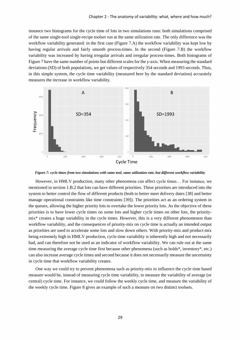
instance two histograms for the cycle time of lots in two simulations runs: both simulations comprised
of the same single-tool single-recipe toolset run at the same utilization rate. The only difference was the
workflow variability generated: in the first case (Figure 7.A) the workflow variability was kept low by
having regular arrivals and fairly smooth process-times. In the second (Figure 7.B) the workflow
variability was increased by having irregular arrivals and irregular process-times. Both histograms of
Figure 7 have the same number of points but different scales for the y-axis. When measuring the standard
deviations (SD) of both populations, we get values of respectively 354 seconds and 1993 seconds. Thus,
in this simple system, the cycle time variability (measured here by the standard deviation) accurately
measures the increase in workflow variability.
Figure 7: cycle times from two simulations with same tool, same utilization rate, but different workflow variability
However, in HMLV production, many other phenomena can affect cycle times… For instance, we
mentioned in section 1.B.2 that lots can have different priorities. These priorities are introduced into the
system to better control the flow of different products (both to better meet delivery dates [38] and better
manage operational constraints like time constraints [39]). The priorities act as an ordering system in
the queues, allowing the higher priority lots to overtake the lower priority lots. As the objective of these
priorities is to have lower cycle times on some lots and higher cycle times on other lots, the priority-
mix* creates a huge variability in the cycle times. However, this is a very different phenomenon than
workflow variability, and the consequences of priority-mix on cycle time is actually an intended output
as priorities are used to accelerate some lots and slow down others. With priority-mix and product-mix
being extremely high in HMLV production, cycle time variability is inherently high and not necessarily
bad, and can therefore not be used as an indicator of workflow variability. We can rule out at the same
time measuring the average cycle time first because other phenomena (such as holds*, inventory*, etc.)
can also increase average cycle times and second because it does not necessarily measure the uncertainty
in cycle time that workflow variability creates.
One way we could try to prevent phenomena such as priority-mix to influence the cycle time based
measure would be, instead of measuring cycle time variability, to measure the variability of average (or
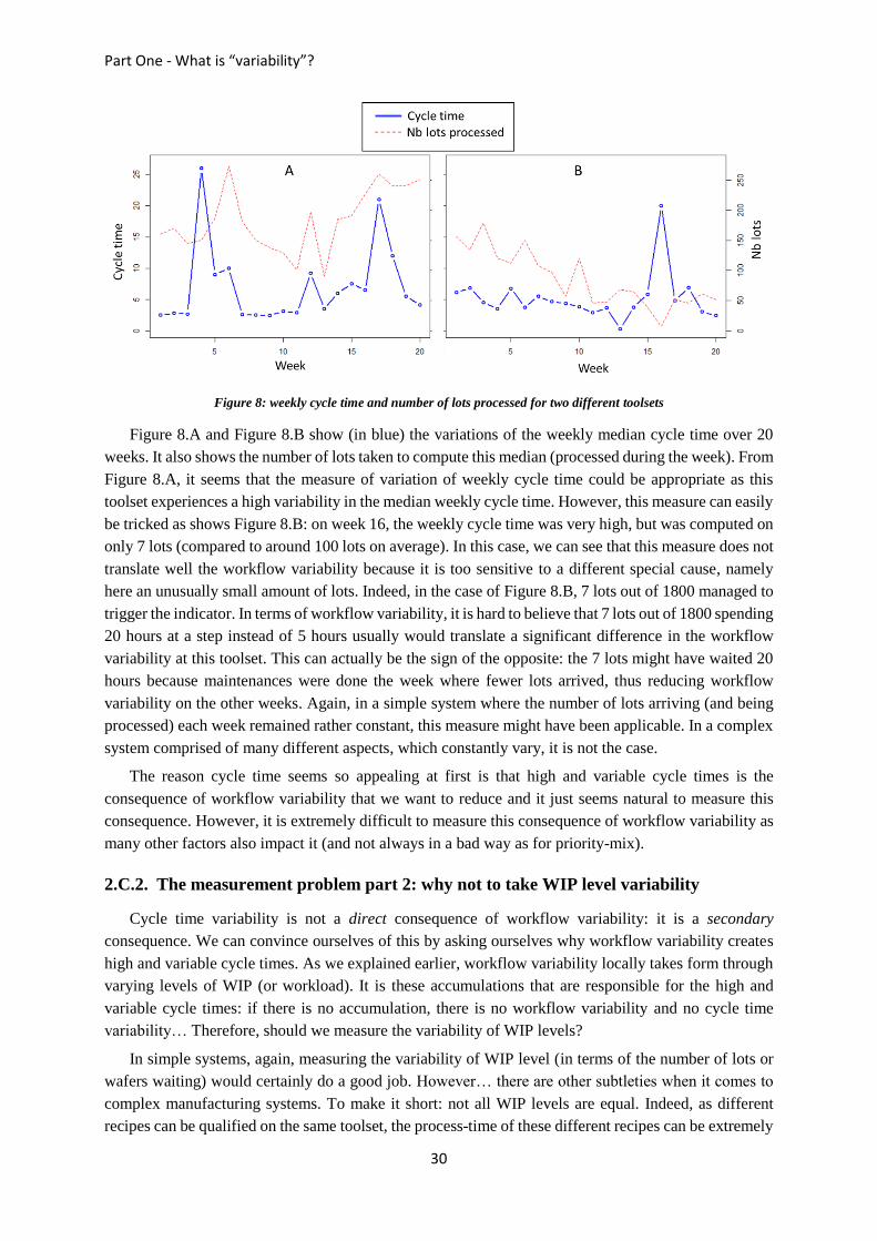
central) cycle time. For instance, we could follow the weekly cycle time, and measure the variability of
the weekly cycle time. Figure 8 gives an example of such a measure on two distinct toolsets.
Part One - What is “variability”?
30
Figure 8: weekly cycle time and number of lots processed for two different toolsets
Figure 8.A and Figure 8.B show (in blue) the variations of the weekly median cycle time over 20
weeks. It also shows the number of lots taken to compute this median (processed during the week). From
Figure 8.A, it seems that the measure of variation of weekly cycle time could be appropriate as this
toolset experiences a high variability in the median weekly cycle time. However, this measure can easily
be tricked as shows Figure 8.B: on week 16, the weekly cycle time was very high, but was computed on
only 7 lots (compared to around 100 lots on average). In this case, we can see that this measure does not
translate well the workflow variability because it is too sensitive to a different special cause, namely
here an unusually small amount of lots. Indeed, in the case of Figure 8.B, 7 lots out of 1800 managed to
trigger the indicator. In terms of workflow variability, it is hard to believe that 7 lots out of 1800 spending
20 hours at a step instead of 5 hours usually would translate a significant difference in the workflow
variability at this toolset. This can actually be the sign of the opposite: the 7 lots might have waited 20
hours because maintenances were done the week where fewer lots arrived, thus reducing workflow
variability on the other weeks. Again, in a simple system where the number of lots arriving (and being
processed) each week remained rather constant, this measure might have been applicable. In a complex
system comprised of many different aspects, which constantly vary, it is not the case.
The reason cycle time seems so appealing at first is that high and variable cycle times is the
consequence of workflow variability that we want to reduce and it just seems natural to measure this
consequence. However, it is extremely difficult to measure this consequence of workflow variability as
many other factors also impact it (and not always in a bad way as for priority-mix).
2.C.2. The measurement problem part 2: why not to take WIP level variability
Cycle time variability is not a direct consequence of workflow variability: it is a secondary
consequence. We can convince ourselves of this by asking ourselves why workflow variability creates
high and variable cycle times. As we explained earlier, workflow variability locally takes form through
varying levels of WIP (or workload). It is these accumulations that are responsible for the high and
variable cycle times: if there is no accumulation, there is no workflow variability and no cycle time
variability… Therefore, should we measure the variability of WIP levels?
In simple systems, again, measuring the variability of WIP level (in terms of the number of lots or
wafers waiting) would certainly do a good job. However… there are other subtleties when it comes to
complex manufacturing systems. To make it short: not all WIP levels are equal. Indeed, as different
recipes can be qualified on the same toolset, the process-time of these different recipes can be extremely
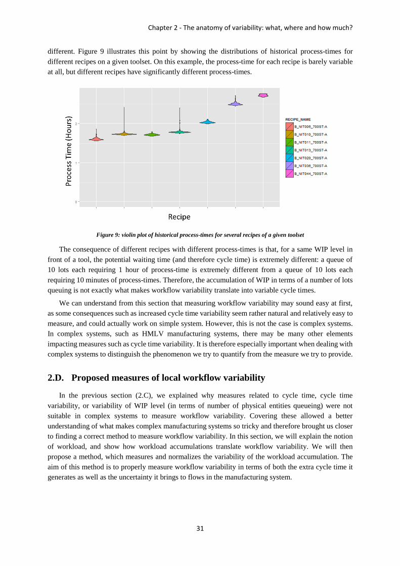
Chapter 2 - The anatomy of variability: what, where and how much?
31
different. Figure 9 illustrates this point by showing the distributions of historical process-times for
different recipes on a given toolset. On this example, the process-time for each recipe is barely variable
at all, but different recipes have significantly different process-times.
Figure 9: violin plot of historical process-times for several recipes of a given toolset
The consequence of different recipes with different process-times is that, for a same WIP level in
front of a tool, the potential waiting time (and therefore cycle time) is extremely different: a queue of
10 lots each requiring 1 hour of process-time is extremely different from a queue of 10 lots each
requiring 10 minutes of process-times. Therefore, the accumulation of WIP in terms of a number of lots
queuing is not exactly what makes workflow variability translate into variable cycle times.
We can understand from this section that measuring workflow variability may sound easy at first,
as some consequences such as increased cycle time variability seem rather natural and relatively easy to
measure, and could actually work on simple system. However, this is not the case is complex systems.
In complex systems, such as HMLV manufacturing systems, there may be many other elements
impacting measures such as cycle time variability. It is therefore especially important when dealing with
complex systems to distinguish the phenomenon we try to quantify from the measure we try to provide.
2.D. Proposed measures of local workflow variability
In the previous section (2.C), we explained why measures related to cycle time, cycle time
variability, or variability of WIP level (in terms of number of physical entities queueing) were not
suitable in complex systems to measure workflow variability. Covering these allowed a better
understanding of what makes complex manufacturing systems so tricky and therefore brought us closer
to finding a correct method to measure workflow variability. In this section, we will explain the notion
of workload, and show how workload accumulations translate workflow variability. We will then
propose a method, which measures and normalizes the variability of the workload accumulation. The
aim of this method is to properly measure workflow variability in terms of both the extra cycle time it
generates as well as the uncertainty it brings to flows in the manufacturing system.
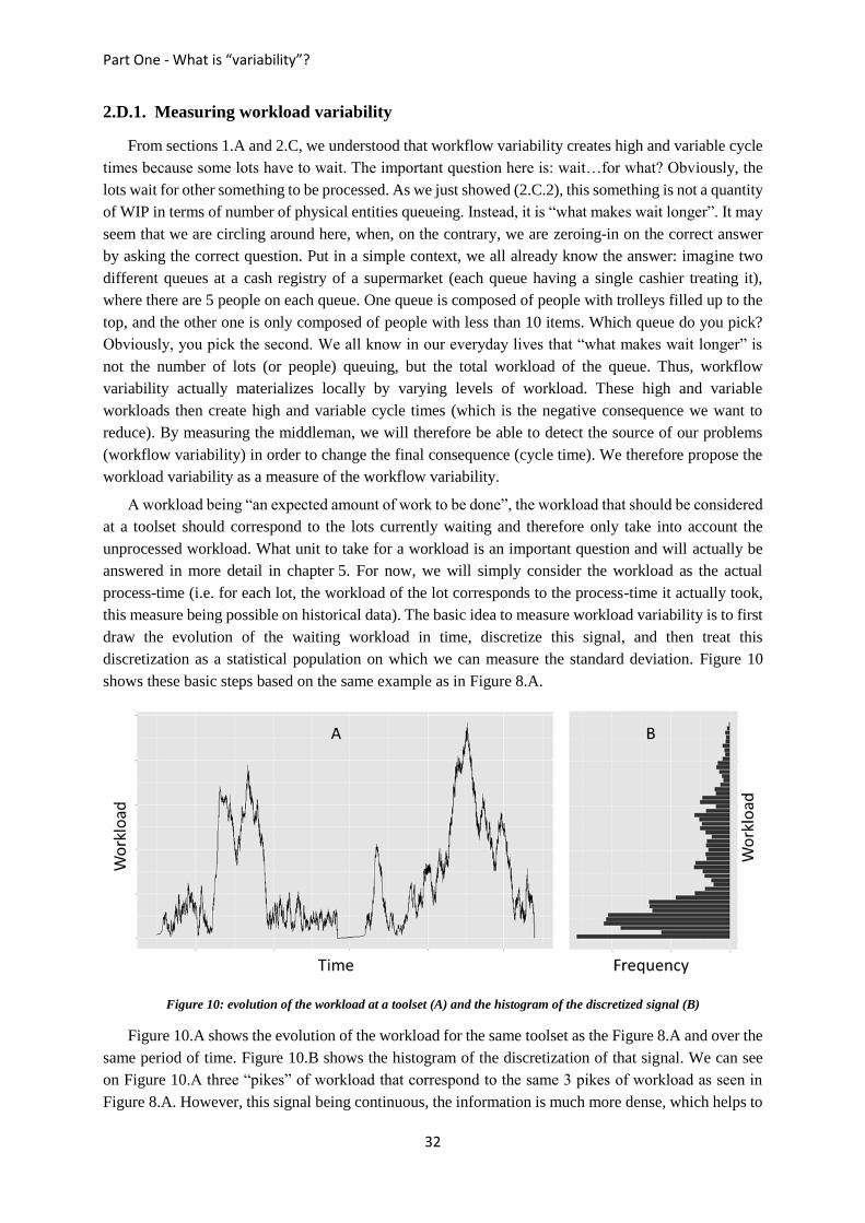
Part One - What is “variability”?
32
2.D.1. Measuring workload variability
From sections 1.A and 2.C, we understood that workflow variability creates high and variable cycle
times because some lots have to wait. The important question here is: wait…for what? Obviously, the
lots wait for other something to be processed. As we just showed (2.C.2), this something is not a quantity
of WIP in terms of number of physical entities queueing. Instead, it is “what makes wait longer”. It may
seem that we are circling around here, when, on the contrary, we are zeroing-in on the correct answer
by asking the correct question. Put in a simple context, we all already know the answer: imagine two
different queues at a cash registry of a supermarket (each queue having a single cashier treating it),
where there are 5 people on each queue. One queue is composed of people with trolleys filled up to the
top, and the other one is only composed of people with less than 10 items. Which queue do you pick?
Obviously, you pick the second. We all know in our everyday lives that “what makes wait longer” is
not the number of lots (or people) queuing, but the total workload of the queue. Thus, workflow
variability actually materializes locally by varying levels of workload. These high and variable
workloads then create high and variable cycle times (which is the negative consequence we want to
reduce). By measuring the middleman, we will therefore be able to detect the source of our problems
(workflow variability) in order to change the final consequence (cycle time). We therefore propose the
workload variability as a measure of the workflow variability.
A workload being “an expected amount of work to be done”, the workload that should be considered
at a toolset should correspond to the lots currently waiting and therefore only take into account the
unprocessed workload. What unit to take for a workload is an important question and will actually be
answered in more detail in chapter 5. For now, we will simply consider the workload as the actual
process-time (i.e. for each lot, the workload of the lot corresponds to the process-time it actually took,
this measure being possible on historical data). The basic idea to measure workload variability is to first
draw the evolution of the waiting workload in time, discretize this signal, and then treat this
discretization as a statistical population on which we can measure the standard deviation. Figure 10
shows these basic steps based on the same example as in Figure 8.A.
Figure 10: evolution of the workload at a toolset (A) and the histogram of the discretized signal (B)
Figure 10.A shows the evolution of the workload for the same toolset as the Figure 8.A and over the
same period of time. Figure 10.B shows the histogram of the discretization of that signal. We can see
on Figure 10.A three “pikes” of workload that correspond to the same 3 pikes of workload as seen in
Figure 8.A. However, this signal being continuous, the information is much more dense, which helps to
Chapter 2 - The anatomy of variability: what, where and how much?
33
the interpretation: on three different occasions, there was an accumulation of workload in front of the
toolset, leading to lots having to wait for this workload to be processed and therefore leading to lots
experiencing higher cycle times. The histogram of Figure 10.B is drawn sideways in order to help the
understanding of what it represents: the “frequency” of each workload interval is the relative amount of
time this amount of workload has been seen waiting at the toolset.
Qualitatively, we can understand through the example of Figure 10 how the population of Figure
10.B is able to translate the workflow variability: workflow variability is only impactful if it creates
higher cycle times, which sit can do through unexpected accumulations of workload. The first important
aspect of this accumulation is “how much”, i.e. the quantity of workload accumulated (a.k.a. the y-axis
of Figure 10.A). The second important aspect however is time: indeed, if a high workload accumulates
just for a few seconds, it is non-impactful, and the longer it accumulates, the more impactful it becomes.
This second dimension is captured in the discretization of the signal: if a given amount of workload
happens longer, there are more time intervals with this amount of workload and the frequency at this
workload in Figure 10.B will be higher. From there, we can understand how the spread of the discretized
workload in Figure 10.B translates the “pikes” of workload in time. This “spreadness” can then be
measured with standard statistics such as the standard deviation.
Note that the workload variability we talk about here is different than the workload variability
addressed by [40]. They addressed differences in total workload processed by different tools within a
toolset, whereas we address the differences in time of the workload waiting to be processed at a toolset.
2.D.2. Normalized measures of workload variability
The need for normalization
The general idea being defined by the previous section (2.D.1), it is now important to choose the
proper units for the value to calculate. Indeed, the raw workload unit (time of process to be done) allows
measuring workflow variability at a given toolset and changes in that variability. It also allows
comparing workflow variability between two different toolsets that are identical in their structure.
However, the comparison is impossible with the raw units when toolsets are different. To understand
this, let us take another example: imagine you are in Disneyland Paris and have to choose between
Pirates of the Caribbean and Peter Pan for the next attraction. As you are physically at neither of them,
you cannot see the instantaneous queues and need to make a decision based on the analysis of historical
data (which you “magically” have). You want to use your knowledge in workflow variability to pick the
ride with the least workflow variability. The measure of section 2.D.1 applied to the historical queues
of both rides tells you that there is a workload standard deviation of 1000 minutes-of-ride at Pirates of
the Caribbean and 200 minutes-of-ride at Peter Pan (the raw units here, minutes-of-ride, are analogous
to minutes-of-process). The question here is: can you decide which attraction to choose only with this
information? As both attractions have different capacities and different riding-times (process-times),
you cannot compare the values between both attractions, as there is not enough information to make a
decision. In order to decide which attraction to choose, you need to normalize these values (i.e. add
information) based on what you actually want. From an industrial standpoint, the problem is similar:
different toolsets have different characteristics and these differences make the raw values of “workload
variability” meaningless when it comes to comparing toolsets. We therefore need to normalize the values
of workload variability in order for it to translate workflow variability. This example is not a direct
analogy to what happens in reality, but serves to illustrate how workload variability can be compared
between two distinct toolsets.

Part One - What is “variability”?
34
In the rest of this section, we will keep the Disneyland example to introduce two normalizations that
allow translating actual workflow variability. These two normalizations, described by Equation (2) and
Equation (3), will then be applied on industrial data from two toolsets from STMicroelectronics in order
to understand their importance in an industrial context.
WaitTime Workload
One main consequence of workflow variability is the uncertainty it generates in the flow and
therefore the decreased tractability of the system. What makes this uncertainty impactful is that some
lots may wait unexpectedly much longer than usual. In this sense, from a tractability point-of-view, what
is important in workflow variability is the variations in absolute cycle time it generates. When
comparing two toolsets between them, this aspect should therefore be compared. For instance, if there
are two operations with uncertain waiting times, one with times ranging from 30min to 1h, the other
ranging from 12h to 24h, the second operation will create much more uncertainty in the flow. If we had
to choose one operation to reduce workflow variability, from the uncertainty point-of-view, we would
choose the second one. In order to measure this consequence of workflow variability, we therefore need
to translate the variations of workload into variations in time. As the “time” consequence of workload
is “queuing time”, the first normalization we propose is to transform workload into “WaitTime
Workload” (WTWL). Equation (2) shows the transformation needed to normalize the Workload unit
into a WaitTime Workload.
𝑊𝑇𝑊𝐿 =
𝑊𝐿
𝑊𝐿̅̅ ̅̅̅× 𝑊𝑇̅̅ ̅̅ ̅ (2)
Fundamentally, the normalization is just dividing the workload (𝑊𝐿) by the average workload 𝑊𝐿̅̅̅̅̅
on the period, and then re-multiplying by the average Waiting-Time on the period (𝑊𝑇̅̅ ̅̅ ̅).
Let us use the context of the Disneyland example to illustrate this. Imagine that you need to order a
taxi for after the ride: you can order the taxi for whatever time, but you do not want to have to wait for
the taxi too long and the taxi will not wait long for you either. So the more certain you are (in absolute
terms) of the total time the ride will take, the better. Obviously, you are not allowed to directly look at
historical cycle time variations as, as explained in section 2.C.1, we cannot do so in complex systems.
You therefore need to normalize the workload variations we previously gave (i.e standard deviation of
1000 minutes-of-ride at Pirates of the Caribbean and 200 minutes-of-ride at Peter Pan) into a waiting-
time dimension. To do so, we need to divide the workload standard deviation values by the average
workload, and then multiply by the average waiting-time (Equation (2)). The average workloads at both
attractions (the average queue-length expressed not in number of people but in riding-time) are 8000
minutes-of-ride for Pirates of the Caribbean and 600 minutes-of-ride for Peter Pan, and the average
waiting-times at both attractions are respectively of 32 and 27 minutes. By applying Equation (2), we
get values of (1000
8000) × 32 = 4 minutes for Pirates of the Caribbean and of (
200
600) × 27 = 9 minutes for
Peter Pan. Therefore, because of workflow variability, workload variability occurs, which gives a
“standard uncertainty” in the queuing time of 4 minutes for Pirates of the Caribbean and 9 minutes for
Peter Pan. In this context, we can conclude that the Peter Pan attraction has more workflow variability
in terms on uncertainty in the flow, and you should therefore choose to ride Pirates of the Caribbean to
have higher chances of catching your taxi.
Chapter 2 - The anatomy of variability: what, where and how much?
35
XFactor Workload
The other main impact of workflow variability is that it creates more time that is non-productive. As
we explained in chapter 1 (1.A.5), we define non-productive time in manufacturing activities in terms
of Xfactor (i.e. the ratio of cycle-time to process-time). Therefore, in order to measure workflow
variability in terms of non-productive time, we need our measure to be expressed as an Xfactor. The
second normalization we propose is therefore to transform workload into “XFactor Workload” (XFWL).
Equation (3) shows the transformation needed to normalize the Workload unit into an Xfactor
Workload.
𝑋𝐹𝑊𝐿 =
𝑊𝐿
𝑊𝐿̅̅ ̅̅̅× (𝑋𝐹̅̅ ̅̅ − 1) + 1 (3)
In order to transform the scale from a workload (WL) to an Xfactor Workload (XFWL), we need to
divide the workload (WL) by the average workload on the period (𝑊𝐿̅̅̅̅̅), multiply it by the average
Xfactor on the period to which we previously removed 1, and finally add 1. The reason we remove 1 to
the Xfactor and then add 1 to the workload is that the workload is only responsible for the waiting-time
part of the Xfactor. Let us illustrate this with an example: imagine that a given toolset has an average
workload of 2 hours-of-process and an average Xfactor of 3. At one point in time, we measure a
queueing workload of 10 hours-of-process: how does this translate in terms of Xfactor? In other words,
if a lot has to wait behind a workload of 10 hours-of-process at this toolset, what is his expected Xfactor?
Even though it experiences 5 times the average workload, it does not have an Xfactor 5 times greater.
The average Xfactor of 3 means that, on average, the sum of waiting-time and process-time equals to 3
times the process-time (𝑊𝑇+𝑃𝑇
𝑃𝑇= 3), which means that the waiting-time equals double the process-time
(𝑊𝑇 = 2𝑃𝑇). When there is 5 times more workload, the waiting-time is 5 times greater, and we
therefore have an Xfactor of 10𝑃𝑇+𝑃𝑇
𝑃𝑇= 11, which we can compute with Equation (3): (
10
2) × (3 − 1) +
1 = 11.
To illustrate the usefulness of this second normalization, let us go back to the Disneyland example.
This time, you want your day to be worth the money. You therefore follow efficiency, which you
measure by how much time of ride you get out of each minute at the attraction: your Xfactor translates
into the cycle-time per minute-of-ride ratio. From this perspective, getting a bad Xfactor ratio on your
next ride would really ruin your day. Therefore, you want to lower this risk and to choose the attraction
with the lowest deviations of Xfactor. Once again, even though in a simple system, we could answer
this question by looking directly at the Xfactor of individuals, we forbid this here as other parameters
affect cycle time in complex systems (see 2.C). We therefore need to rely on the workload variations
and normalize the workload variations relative to the Xfactor by following Equation (3): we will first
divide the workload standard deviation values (that we previously obtained) by the average workload,
and then transform to an Xfactor. The average workload at both attractions are 8000 minutes-of-ride for
Pirates of the Caribbean and 600 minutes-of-ride for Peter Pan, the average ride-time is 8 minutes for
Pirates of the Caribbean and 3 minutes for Peter Pan, and the average cycle times are respectively 40
minutes and 30 minutes. This later information means that Pirates of the Caribbean has an average
Xfactor of 5, and Peter Pan an average Xfactor of 10. Dividing both workload standard deviations by
the average workload and transforming them back into an Xfactor gives us equivalent standard
deviations of (1000
8000) × (5 − 1) = 0.5 for Pirates of the Caribbean and (
200
600) × (10 − 1) = 3 for Peter
Pan (Note that we did not add 1 at the end of the normalization here as we here normalized the standard
deviation and not the scale). Therefore, because of workflow variability, the workload variability that
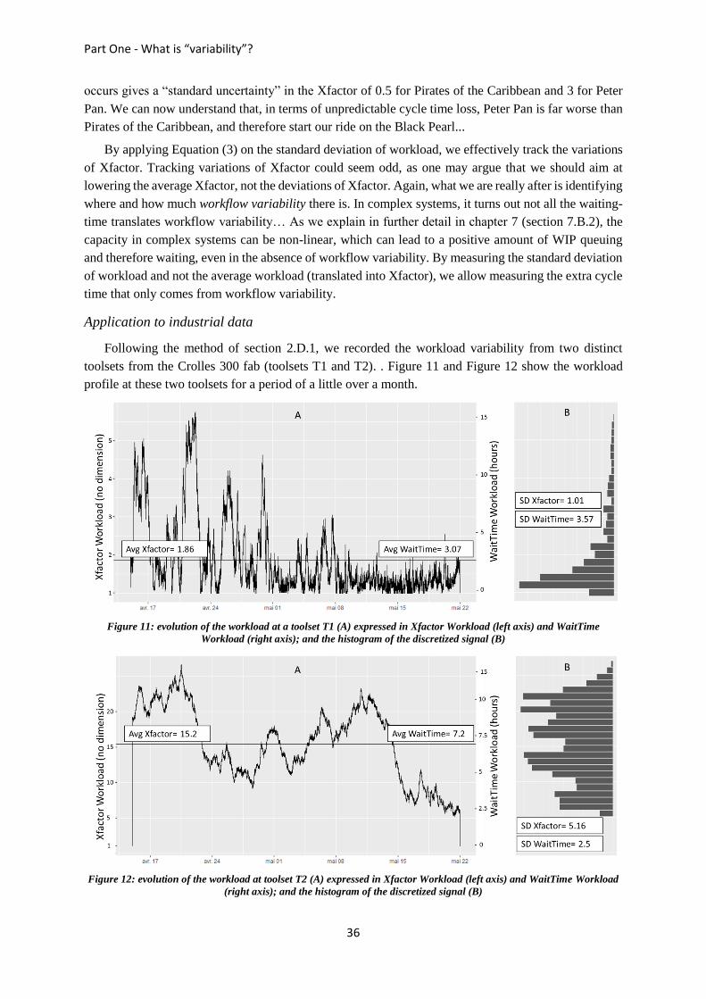
Part One - What is “variability”?
36
occurs gives a “standard uncertainty” in the Xfactor of 0.5 for Pirates of the Caribbean and 3 for Peter
Pan. We can now understand that, in terms of unpredictable cycle time loss, Peter Pan is far worse than
Pirates of the Caribbean, and therefore start our ride on the Black Pearl...
By applying Equation (3) on the standard deviation of workload, we effectively track the variations
of Xfactor. Tracking variations of Xfactor could seem odd, as one may argue that we should aim at
lowering the average Xfactor, not the deviations of Xfactor. Again, what we are really after is identifying
where and how much workflow variability there is. In complex systems, it turns out not all the waiting-
time translates workflow variability… As we explain in further detail in chapter 7 (section 7.B.2), the
capacity in complex systems can be non-linear, which can lead to a positive amount of WIP queuing
and therefore waiting, even in the absence of workflow variability. By measuring the standard deviation
of workload and not the average workload (translated into Xfactor), we allow measuring the extra cycle
time that only comes from workflow variability.
Application to industrial data
Following the method of section 2.D.1, we recorded the workload variability from two distinct
toolsets from the Crolles 300 fab (toolsets T1 and T2). . Figure 11 and Figure 12 show the workload
profile at these two toolsets for a period of a little over a month.
Figure 11: evolution of the workload at a toolset T1 (A) expressed in Xfactor Workload (left axis) and WaitTime
Workload (right axis); and the histogram of the discretized signal (B)
Figure 12: evolution of the workload at toolset T2 (A) expressed in Xfactor Workload (left axis) and WaitTime Workload
(right axis); and the histogram of the discretized signal (B)
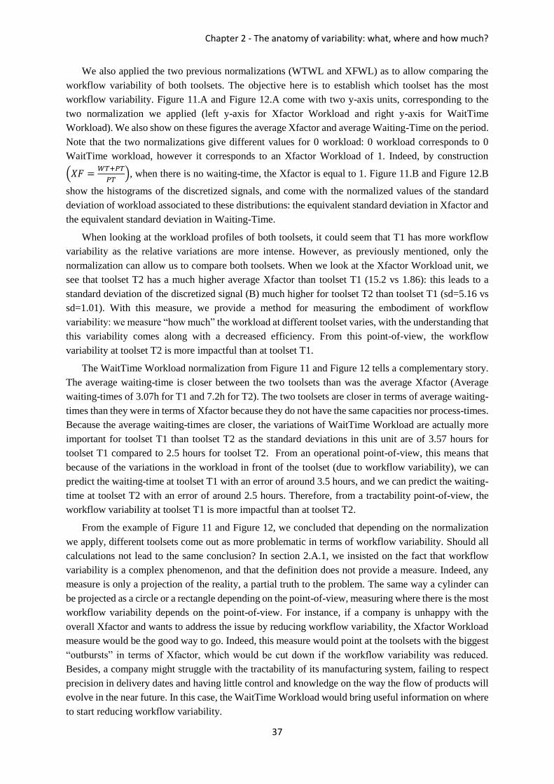
Chapter 2 - The anatomy of variability: what, where and how much?
37
We also applied the two previous normalizations (WTWL and XFWL) as to allow comparing the
workflow variability of both toolsets. The objective here is to establish which toolset has the most
workflow variability. Figure 11.A and Figure 12.A come with two y-axis units, corresponding to the
two normalization we applied (left y-axis for Xfactor Workload and right y-axis for WaitTime
Workload). We also show on these figures the average Xfactor and average Waiting-Time on the period.
Note that the two normalizations give different values for 0 workload: 0 workload corresponds to 0
WaitTime workload, however it corresponds to an Xfactor Workload of 1. Indeed, by construction
(𝑋𝐹 =𝑊𝑇+𝑃𝑇
𝑃𝑇), when there is no waiting-time, the Xfactor is equal to 1. Figure 11.B and Figure 12.B
show the histograms of the discretized signals, and come with the normalized values of the standard
deviation of workload associated to these distributions: the equivalent standard deviation in Xfactor and
the equivalent standard deviation in Waiting-Time.
When looking at the workload profiles of both toolsets, it could seem that T1 has more workflow
variability as the relative variations are more intense. However, as previously mentioned, only the
normalization can allow us to compare both toolsets. When we look at the Xfactor Workload unit, we
see that toolset T2 has a much higher average Xfactor than toolset T1 (15.2 vs 1.86): this leads to a
standard deviation of the discretized signal (B) much higher for toolset T2 than toolset T1 (sd=5.16 vs
sd=1.01). With this measure, we provide a method for measuring the embodiment of workflow
variability: we measure “how much” the workload at different toolset varies, with the understanding that
this variability comes along with a decreased efficiency. From this point-of-view, the workflow
variability at toolset T2 is more impactful than at toolset T1.
The WaitTime Workload normalization from Figure 11 and Figure 12 tells a complementary story.
The average waiting-time is closer between the two toolsets than was the average Xfactor (Average
waiting-times of 3.07h for T1 and 7.2h for T2). The two toolsets are closer in terms of average waiting-
times than they were in terms of Xfactor because they do not have the same capacities nor process-times.
Because the average waiting-times are closer, the variations of WaitTime Workload are actually more
important for toolset T1 than toolset T2 as the standard deviations in this unit are of 3.57 hours for
toolset T1 compared to 2.5 hours for toolset T2. From an operational point-of-view, this means that
because of the variations in the workload in front of the toolset (due to workflow variability), we can
predict the waiting-time at toolset T1 with an error of around 3.5 hours, and we can predict the waiting-
time at toolset T2 with an error of around 2.5 hours. Therefore, from a tractability point-of-view, the
workflow variability at toolset T1 is more impactful than at toolset T2.
From the example of Figure 11 and Figure 12, we concluded that depending on the normalization
we apply, different toolsets come out as more problematic in terms of workflow variability. Should all
calculations not lead to the same conclusion? In section 2.A.1, we insisted on the fact that workflow
variability is a complex phenomenon, and that the definition does not provide a measure. Indeed, any
measure is only a projection of the reality, a partial truth to the problem. The same way a cylinder can
be projected as a circle or a rectangle depending on the point-of-view, measuring where there is the most
workflow variability depends on the point-of-view. For instance, if a company is unhappy with the
overall Xfactor and wants to address the issue by reducing workflow variability, the Xfactor Workload
measure would be the good way to go. Indeed, this measure would point at the toolsets with the biggest
“outbursts” in terms of Xfactor, which would be cut down if the workflow variability was reduced.
Besides, a company might struggle with the tractability of its manufacturing system, failing to respect
precision in delivery dates and having little control and knowledge on the way the flow of products will
evolve in the near future. In this case, the WaitTime Workload would bring useful information on where
to start reducing workflow variability.

Part One - What is “variability”?
38
2.E. Decomposing a manufacturing system into local process-clusters
In the previous sections of chapter 2, we established that we should (and could) measure workflow
variability at the toolset level. However, we did not provide a definition for a toolset. This might seem
like a trivial problem, as toolset are commonly agreed to simply be groups of tools treating the same
products. In complex systems however, this definition has grey areas as flexibility* and tool dedication*
make unclear what “same” really means. We will show in this section that the notion of “toolset” is
problematic and does not allow properly splitting a manufacturing system to study its characteristics.
We will then propose a new notion, called process-clusters, which allows a rigorous grouping of process-
units (whether it is tools, machines, servers…) in any manufacturing system or queuing system, based
on the connections between the process-units through the flow of products. As we will show that not all
connections between process-units are equal, we will go one-step further by defining “highly connected
process-clusters”, i.e. a grouping of process-units based on the flow treated that translates the ability of
tools to rely on each other, a grouping which can be calculated on any manufacturing system.
2.E.1. Defining process-clusters
Transitioning to generic terms
Our objective in this section is to make groups of processing entities in a manufacturing system,
which, as we will show, cannot rely on the simple notion of “tools treating the same queue” in complex
systems. As this grouping problem is very generic and can arise in any system with queue-like structures,
we will define the notions with generic terms. Therefore, we will define process-units as the entities
performing tasks (whether it is tools, chambers, operators, robots, cashiers…), jobs* as the entities on
which the tasks are performed (whether it is lots, products, clients, cars…) and job-families* as jobs
with same characteristics from the process-units point-of-view (that can be defined as a recipe, a
product-type*, a client-type…). The explanations in this section are based on an example of tools
processing lots from different recipes, but is applicable to any groups of process-units treating jobs of
different job-families.
The problem with fixed toolsets
The first step to measure local workload variability of a system is to find the proper local aggregation
of process-units (tools, chambers, operators, robots, cashiers…). This grouping seems fairly obvious at
first, as the notion of toolsets (that arises when regarding questions of capacity, cycle time, and
throughput) seems pretty clear: the process-units that treat the same jobs (whether it is lots, products,
clients, cars…), or from a queuing theory point-of-view, the process-units that treat the same queue of
jobs. In our everyday life examples, this definition seems satisfying: if cashiers treat individual queues,
the “toolsets” are individual cashiers, if several cashiers treat a single queue (as in IKEA), the “toolset”
is all the cashiers that treat the same queue of customers. In complex manufacturing systems however,
this concept of individual queues can faint out rather quickly, because of what is called “flexibility”.
Flexibility, as described by Gurumurthi and Benjaafar [41], is the possibility for different job-families
(jobs with same characteristics from the process-units point-of-view), to be processed by more than one
process-unit and the possibility for process-units to process more than one job-family.
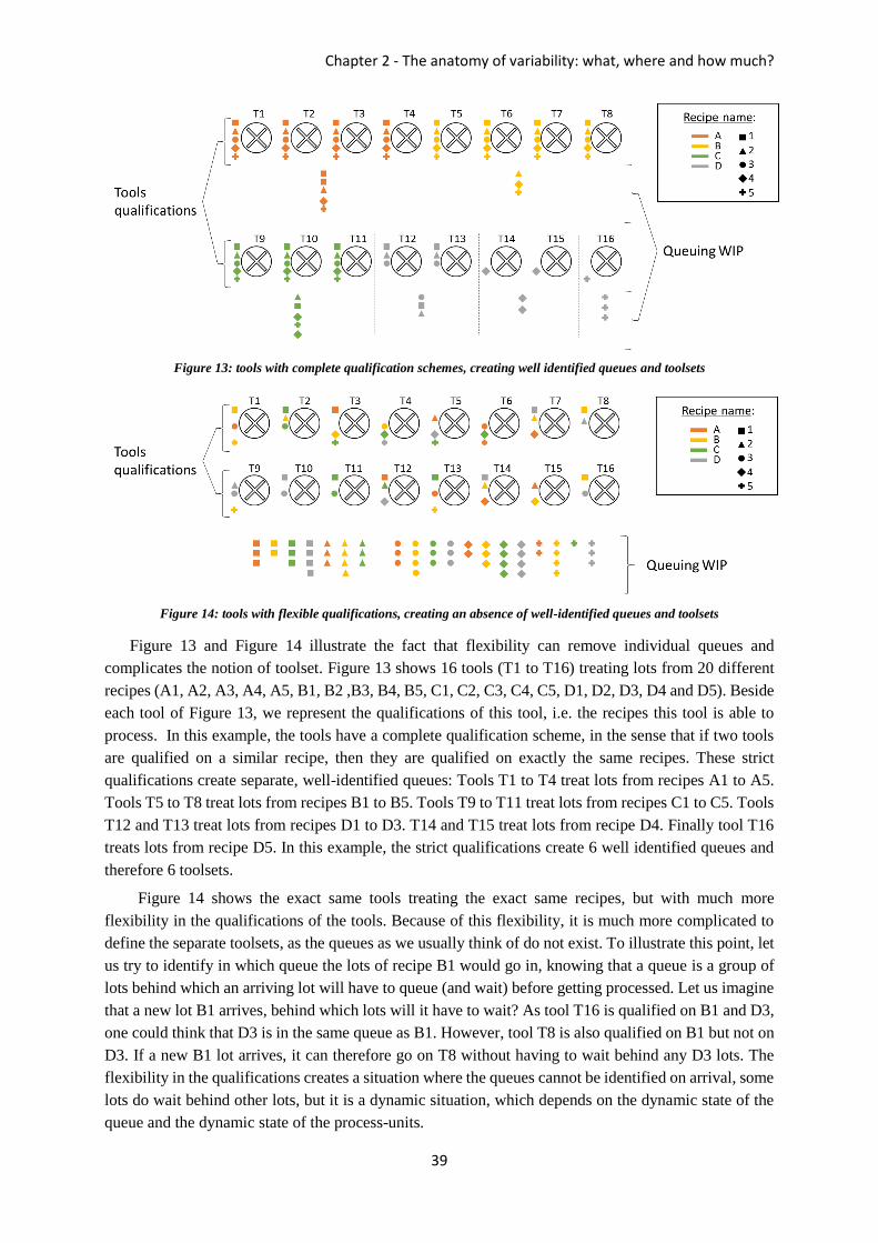
Chapter 2 - The anatomy of variability: what, where and how much?
39
Figure 13: tools with complete qualification schemes, creating well identified queues and toolsets
Figure 14: tools with flexible qualifications, creating an absence of well-identified queues and toolsets
Figure 13 and Figure 14 illustrate the fact that flexibility can remove individual queues and
complicates the notion of toolset. Figure 13 shows 16 tools (T1 to T16) treating lots from 20 different
recipes (A1, A2, A3, A4, A5, B1, B2 ,B3, B4, B5, C1, C2, C3, C4, C5, D1, D2, D3, D4 and D5). Beside
each tool of Figure 13, we represent the qualifications of this tool, i.e. the recipes this tool is able to
process. In this example, the tools have a complete qualification scheme, in the sense that if two tools
are qualified on a similar recipe, then they are qualified on exactly the same recipes. These strict
qualifications create separate, well-identified queues: Tools T1 to T4 treat lots from recipes A1 to A5.
Tools T5 to T8 treat lots from recipes B1 to B5. Tools T9 to T11 treat lots from recipes C1 to C5. Tools
T12 and T13 treat lots from recipes D1 to D3. T14 and T15 treat lots from recipe D4. Finally tool T16
treats lots from recipe D5. In this example, the strict qualifications create 6 well identified queues and
therefore 6 toolsets.
Figure 14 shows the exact same tools treating the exact same recipes, but with much more
flexibility in the qualifications of the tools. Because of this flexibility, it is much more complicated to
define the separate toolsets, as the queues as we usually think of do not exist. To illustrate this point, let
us try to identify in which queue the lots of recipe B1 would go in, knowing that a queue is a group of
lots behind which an arriving lot will have to queue (and wait) before getting processed. Let us imagine
that a new lot B1 arrives, behind which lots will it have to wait? As tool T16 is qualified on B1 and D3,
one could think that D3 is in the same queue as B1. However, tool T8 is also qualified on B1 but not on
D3. If a new B1 lot arrives, it can therefore go on T8 without having to wait behind any D3 lots. The
flexibility in the qualifications creates a situation where the queues cannot be identified on arrival, some
lots do wait behind other lots, but it is a dynamic situation, which depends on the dynamic state of the
queue and the dynamic state of the process-units.
Part One - What is “variability”?
40
As each tool in a semiconductor fab is qualified on dozens (or even hundreds) of recipes, the actual
queue-like structures in real complex environments get really hard to identify or handle. However, in
order to manage the production (and to measure workflow variability), we need to split the
manufacturing system into local groups of tools… This problematic does not only apply to
semiconductor manufacturing tools and lots. Any manufacturing system made of process-units capable
of performing required activities on incoming flows of jobs with some degree of flexibility will face the
same problems.
In the Crolles300 and Crolles200 fabs, the lack of proper tool grouping was problematic for the
production management activities. Local toolsets were already defined in order to perform capacity
analysis and other industrial engineering activities, however these groupings were made manually,
usually based on the experience and the knowledge of the different teams. This manual grouping has
several downsides. First, the toolsets are generally defined once, for a long period, whereas the product-
mix and qualifications may change over time and make the grouping obsolete. Second, the groupings
do not always follow the same rules, which can cause problems when trying to perform analysis on the
toolsets.
Notion of process-clusters
The important aspect of the notion of queue and toolsets treating an identical queue is that the tools
in the same toolset can compensate for each other. For instance, if a tool has a failure, the other tools in
the toolset can compensate by treating the lots that would normally go on that tool. With flexible
qualifications, this compensation mechanism is still possible. Indeed, if two tools are qualified on the
same recipe and one fails, the other can take more of that recipe (and compensate for the first tool’s
failure). With flexible qualifications, the tools can actually “cascade down” the WIP to compensate for
each other. For instance, in our previous example (Figure 14), tools T3 and T12 are qualified on A1, and
if T3 fails, T12 can take more lots from recipe A1 to compensate for T3. Moreover, if because of this
T12 has too much work to do, it can “focus” on lots A1 and “cascade down” to tool T5 some of the lots
D4 that it would normally do (as T12 and T5 are both qualified on D4). We can therefore see that, at
least, T3, T12, and T5 in our example are part of a same group as they can influence each other through
the incoming workload. By following this concept, we can define a first type of group, process-clusters,
as process-units that can influence each other through the flow of incoming jobs. Process-clusters are
analogous to toolsets treating individual queues (as in Figure 13) as, by definition, process-units from
different process-clusters cannot influence each other through the incoming WIP, and can therefore be
studied separately.
By applying a more rigorous definition (as in [41]) to the principle of connectivity that we just
explained, we can define an individual process-cluster as a set of process-units connected between them
by their job-families qualifications. The term “connected” here refers to connections as in graph-theory.
Indeed, we can represent process-units and job-qualifications as nodes, and each process-unit
qualification as an edge going from a process-unit to a job-qualification. Two process-units are therefore
connected (and part of the same process-cluster) if there is a path in this graph that goes from one of
these process-units to the other. By applying this definition to the previous example (Figure 14), we can
connect all the tools to the recipes they are qualified on, and find the process-clusters that exist in this
example. Figure 15 therefore shows all the connections between the tools and the recipes from the same
example as in Figure 14, and the process-clusters that form from this definition.

Chapter 2 - The anatomy of variability: what, where and how much?
41
Figure 15: two process-groups defined by their tools qualifications
Figure 15 shows the exact same tools and tools qualifications as in Figure 14. In the middle, we
represented each of the recipes that have at least one qualification on a tool. If a tool is qualified on a
recipe, a line is drawn connecting the tool to the recipe. The lines are then colored by a connectivity
principle: all lines that connect a same tool have the same color, and all lines that connect a same recipe
have the same color. In this example, connecting all tools to their qualified recipe created two distinct
process-cluster (P1 and P2) whose connections are drawn in blue and orange. This connectivity principle
also means that, through the connections drawn in Figure 15, we can access any tool belonging to
process-cluster P1 from any other tool belonging to process-cluster P1 (and only from tools belonging
to this process-cluster). For instance, if we want to go from tool T1 to tool T13, we can go through recipe
A3. Some connections however are more difficult to find: can we really go from T1 to T10? To go from
T1 to T10, we actually need to take an indirect path: we can go from T1 to T16 through B1, and then
from T16 to T10 through D3.
Mathematical description
Even though we have a definition for process-clusters, the way we built the process-clusters in
Figure 15 feels rather clumsy. Moreover, the connections between the tools are hard to visualize and
interpret, and the direct connections (like T1/T13) are not easily distinguishable from the indirect
connection (like T1/T10). In order to rigorously draw process-clusters and show the direct and indirect
connections, we can actually use a mathematical description of process-clusters, based on what is called
the qualification matrix. A qualification matrix is a description of process-units qualifications with the
process-units describing rows and the job-families describing columns. If a process-unit i is qualified
on a job-family j, than the value of item 𝑥𝑖,𝑗 is 1, otherwise the value is 0. Figure 16 shows the
qualification matrix (𝑀𝑞) from the tools of Figure 14 and Figure 15. This specific matrix shows tools in
rows and recipes in columns. The qualification matrix 𝑀𝑞 directly links to the previous example (Figure
15): as we can see on the matrix 𝑀𝑞, tools T1 and T13 have two identical qualifications (A3 and B5),
which correspond to two different paths that directly link T1 and T13 in Figure 15.
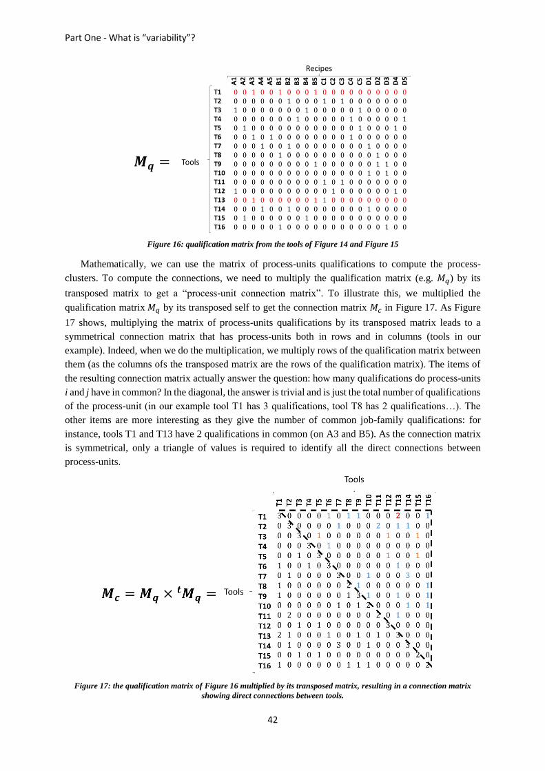
Part One - What is “variability”?
42
Figure 16: qualification matrix from the tools of Figure 14 and Figure 15
Mathematically, we can use the matrix of process-units qualifications to compute the process-
clusters. To compute the connections, we need to multiply the qualification matrix (e.g. 𝑀𝑞) by its
transposed matrix to get a “process-unit connection matrix”. To illustrate this, we multiplied the
qualification matrix 𝑀𝑞 by its transposed self to get the connection matrix 𝑀𝑐 in Figure 17. As Figure
17 shows, multiplying the matrix of process-units qualifications by its transposed matrix leads to a
symmetrical connection matrix that has process-units both in rows and in columns (tools in our
example). Indeed, when we do the multiplication, we multiply rows of the qualification matrix between
them (as the columns ofs the transposed matrix are the rows of the qualification matrix). The items of
the resulting connection matrix actually answer the question: how many qualifications do process-units
i and j have in common? In the diagonal, the answer is trivial and is just the total number of qualifications
of the process-unit (in our example tool T1 has 3 qualifications, tool T8 has 2 qualifications…). The
other items are more interesting as they give the number of common job-family qualifications: for
instance, tools T1 and T13 have 2 qualifications in common (on A3 and B5). As the connection matrix
is symmetrical, only a triangle of values is required to identify all the direct connections between
process-units.
Figure 17: the qualification matrix of Figure 16 multiplied by its transposed matrix, resulting in a connection matrix
showing direct connections between tools.

Chapter 2 - The anatomy of variability: what, where and how much?
43
Now that we have all the direct connections between the tools in the matrix 𝑀𝑐, we can easily draw
them to show the process-clusters without having to draw the recipes. We draw in Figure 18 all the
connections defined by the connection matrix 𝑀𝑐 of Figure 17: if an item i,j from the matrix of Figure
17 has a positive value, then tools Ti and Tj are connected in Figure 18. In this example, there are 26
connections between tools from the 112 possible. By drawing the connections, we brought up to clear
light the two process-clusters (P1 and P2) of our example that we had identified in Figure 15. This time
however, the connections are clear, and the distinction between direct and indirect connections is
obvious. For instance, tools T1 and T13 have a direct connection, whereas tools T1 and T10 only have
indirect connections. In this case, we can actually see that there are many different paths to go from T1
to T10. From the graph of Figure 18, we also understand how the tools of an identical process-cluster
are able to cascade down the workload to compensate for each other.
Figure 18: direct connections between tools, showing two process-clusters
Different qualifications for different types of process-clusters
Process-units qualifications have been defined rather quickly in our previous examples. However,
there is more to qualifications than meets the eye. Indeed, qualifications can mean “the set of job-
families that a process-unit can be able to process”, “the set of job-families that a process-unit can
immediately process”, “the set of job-families that a process-unit effectively processes”… Depending
on what we understand by “qualification”, we will get different types of process-clusters.
As previously mentioned, tool-groups in the Crolles fab were problematic as they did not rely on
rigorous definitions (and computations). Based on the work done with process-clusters, two types of
tool-groups were introduced and are currently in use for the capacity planning activities in the Crolles
fabs. These two tool-groups correspond to the definition of process-clusters, but have different types of
“qualifications”. “Balancing-Groups” is the name given at ST Crolles for process-clusters based on the
possible qualifications of tools, and “Balanced-Groups” is the name given to the process-clusters based
on the qualifications suggested by a balancing algorithm [40]. The main advantage of creating the groups
based on the definition of process-clusters is that the groups define the boundaries for the balancing
algorithm: knowing these boundaries, the problem can be split beforehand to reduce complexity and
allow parallel computation (making the algorithm run faster).
Both tool-groups mentioned above rely on predicted scenarios, predicted flows, and theoretical
qualifications. These groups are therefore made for activities looking at the future. Other activities
however need to look in the past. For instance, in order to make groups to measure workflow variability,
we need the groups to correspond to the past flows of products. To measure workflow variability, we
need to look at the “historical effective qualifications”. That is, we should look all processes done by all
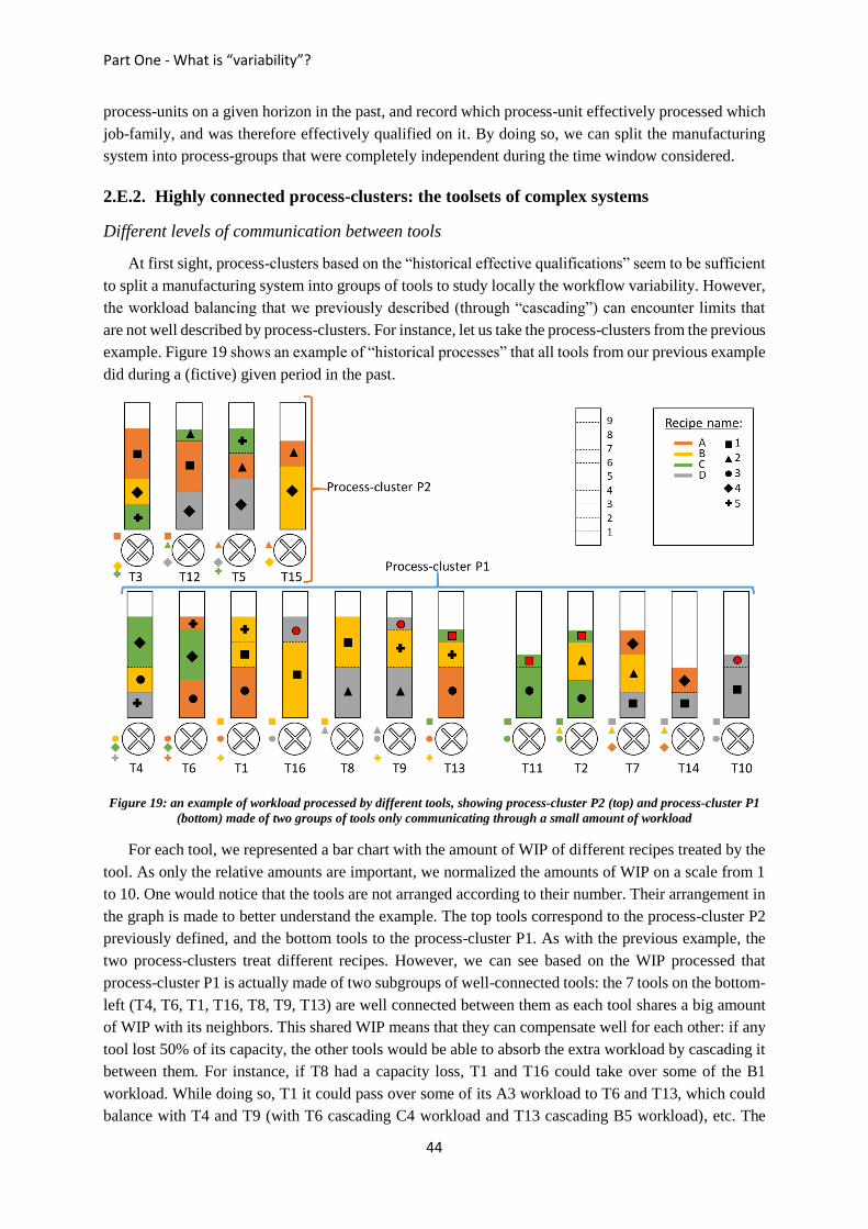
Part One - What is “variability”?
44
process-units on a given horizon in the past, and record which process-unit effectively processed which
job-family, and was therefore effectively qualified on it. By doing so, we can split the manufacturing
system into process-groups that were completely independent during the time window considered.
2.E.2. Highly connected process-clusters: the toolsets of complex systems
Different levels of communication between tools
At first sight, process-clusters based on the “historical effective qualifications” seem to be sufficient
to split a manufacturing system into groups of tools to study locally the workflow variability. However,
the workload balancing that we previously described (through “cascading”) can encounter limits that
are not well described by process-clusters. For instance, let us take the process-clusters from the previous
example. Figure 19 shows an example of “historical processes” that all tools from our previous example
did during a (fictive) given period in the past.
Figure 19: an example of workload processed by different tools, showing process-cluster P2 (top) and process-cluster P1
(bottom) made of two groups of tools only communicating through a small amount of workload
For each tool, we represented a bar chart with the amount of WIP of different recipes treated by the
tool. As only the relative amounts are important, we normalized the amounts of WIP on a scale from 1
to 10. One would notice that the tools are not arranged according to their number. Their arrangement in
the graph is made to better understand the example. The top tools correspond to the process-cluster P2
previously defined, and the bottom tools to the process-cluster P1. As with the previous example, the
two process-clusters treat different recipes. However, we can see based on the WIP processed that
process-cluster P1 is actually made of two subgroups of well-connected tools: the 7 tools on the bottom-
left (T4, T6, T1, T16, T8, T9, T13) are well connected between them as each tool shares a big amount
of WIP with its neighbors. This shared WIP means that they can compensate well for each other: if any
tool lost 50% of its capacity, the other tools would be able to absorb the extra workload by cascading it
between them. For instance, if T8 had a capacity loss, T1 and T16 could take over some of the B1
workload. While doing so, T1 it could pass over some of its A3 workload to T6 and T13, which could
balance with T4 and T9 (with T6 cascading C4 workload and T13 cascading B5 workload), etc. The

Chapter 2 - The anatomy of variability: what, where and how much?
45
same goes for the 5 tools on the bottom-right side (T11, T2, T7, T14, and T10). However, the 7 tools on
the bottom-left and the 5 tools on the bottom-right have very little “communication capability” between
them. Indeed, they are only connected by recipes C1 and D3 (highlighted in red in Figure 19), which
have very small volumes treated. Therefore, only a very small amount of WIP can cascade over from
the tools {T4, T6, T1, T16, T8, T9, T13} to the tools {T11, T2, T7, T14, T10}. Another way of seeing
this is that, by only removing or reallocating a small amount of WIP (recipes C1 and D3), we could have
two separate process-clusters. The definition of process-cluster does not allow to see these differences
and group closer together tools that have bigger “communication channels”. We therefore need a way
to integrate this aspect when grouping tools together.
Building highly connected process-clusters
When creating the process-clusters in Figure 18, we only considered the existence of a connection
between two tools in the connection matrix to draw a link between these tools, but we did not focus at
all on the weight of the edges in the graph (i.e. the value in the connection matrix). When we start with
a classic qualification matrix, the value of the edges tell the number of different recipes connecting two
tools. This is obtained from a qualification matrix with only 1s and 0s in it, for the existence or not of a
qualification. Instead of filling the qualification matrix with 1s and 0s, we can actually give the amounts
of volume treated by each tool on each recipe. By doing so, the values obtained in the result matrix
actually correspond to volumes that can pass from one tool to another through a given recipe. In
layman’s term, we get the size of the pipe that connects the two tools. By applying this to our example,
i.e. starting with a qualification matrix that has values given by the volumes treated as shown in Figure
19, we get values in the connection matrix which allow building a weighted graph as shown in Figure
20. For instance, as T1 and T16 are only connected through B1 with B1 volumes-treated respectively of
2 and 6, their connection’s weight is 2 × 6 = 12. As T7 and T14 both processed products A4 and D1
with volume 2 each time, their connection weight is 2 × 2 + 2 × 2 = 8.
Figure 20: connections between tools taking volumes processed into account
We get in Figure 20 almost the same connections as in Figure 18. The only missing connection is
the connection T2/T14 as, as Figure 19 shows, tool T14 did not process any lot of recipe B2 and therefore
did not have an “effective qualification” on B2. The main difference between Figure 20 and Figure 18
is that we now have weights on the edges of the graph, which represent the level of connection between
the tools. Based on this example, we can get a feeling of what a highly connected process-cluster should
be by doing a simple thought experiment. Let us imagine that the tools are entities attracted to each other
with a force given by the weight of their connections. The thought experiment is to try to break apart

Part One - What is “variability”?
46
the process-cluster by applying a field force (like a magnetic force) on a subgroup of the process-cluster
(We use the notion of “field-force” here to favor grouping tools together: a single tool will be harder to
break apart from its counterparts than a group of tools.). The question becomes: are there strong
structures in the process-cluster, entities that are harder to break apart from each other than others are?
Alternatively, is there a weak-point in the process-cluster? Is there a group of tools that can detach
relatively easily? This thought experiment applied on the process-clusters of Figure 20 would
qualitatively give a weak points to the process-cluster P1: separating the five bottom tools from the top
ones would take the smallest “field-force”, whereas trying to break apart {T16, T9, T13} from the other
tools would take a huge force.
Creating highly connected process-clusters using graph theory
Once again, the highly connected process-clusters that we identified in our previous example do not
have a rigorous definition, as they are so far “visual”. From our though experiment tough, we can
understand what a mathematical description should aim at. We can therefore translate this though
experiment mathematically using graph-theory. Graph clustering is the branch of graph theory that aims
at making clusters of vertices from a single connected graph, with the general idea of clusters being
“dense subgraphs such that a dense subgraph contains more well connected internal edges connecting
the vertices in the subgraph than cutting edges connecting the vertices across subgraphs” [42], which is
qualitatively the real-world problem we face. There are many different measures aimed at evaluating
the quality of a cluster such as intra/inter-cut density, ratio cut, performance, conductance, modularity,
expansion… [42]. These measures are sometimes applied to real-world problems, but are often the
starting point to research aiming at finding the proper algorithms to minimize these measures.
The measure that applies best to our case (finding highly connected process-clusters) would be the
measure of expansion [43]. In graph theory, the expansion of a cut (a cut being a split of a graph into
two groups of vertices) is the sum of the weights of the edges that are cut divided by the cardinality of
the smallest subgroup created. The expansion problem has several formulations, which can for instance
be finding the minimum expansion of a graph, or making clusters that have minimal expansion above a
given value. This last formulation is interesting but arbitrary, as the given value represents something
absolute, not relative. To our knowledge, no graph formulation (and measure) that address fully the
problem that we face exist…
An alternative model that we propose is, instead of putting a condition on the minimum expansion
of a graph, to put a condition on the ratio between the minimum expansion and the maximum expansion
of a graph, which we will call the min-max expansion ratio. In other words, we want to define if a group
of process-units is a highly connected process cluster based on the ratio between the minimum expansion
and the maximum expansion of its graph. Dividing by the maximum expansion of the graph serves as a
normalization for the minimum expansion. This normalization allows comparing the min-max
expansion ratio with a single value, which does not depend on any graph or subgraph, but can be set as
a baseline. We will therefore formulate our clustering problem as follow: from a given graph, keep only
subgraphs with a min-max expansion ratio higher than a given value r. Finding the minimum expansion
of a graph being a NP-hard problem [42], this problem is also at least an NP-hard problem. As there is
a vast literature on minimum expansion, our problem could be solved by adapting classic algorithms
that find separately the minimum expansion and the maximum expansion of a graph.
The highly connected process-clusters would simply be the real world images of the subgraphs that
have min-max expansion ratios higher than a desired r-value. For real-world applications, the value we
put on the ratio r is necessarily somewhat arbitrary. It needs to be set depending on the specific

Chapter 2 - The anatomy of variability: what, where and how much?
47
requirement of the clustering, knowing that the higher the ratio, the higher the connectivity requirement.
From our tests, a ratio of 0.05 gives good results for clustering the tools of the C300 and C200 fab. This
ratio of 0.05 could serve as a baseline for highly connected process-clusters of other applications.
In our previous example (Figure 20), the maximum expansion in process-cluster P1 corresponds to
cutting tool T1, with an expansion value of 58/1 = 58 (the sum of the weights with this cut equals 58,
and the smallest sub-group created by this cut is of cardinality 1) . The minimum expansion corresponds
to cutting off {T2, T7, T10, T11, T14}, with an expansion value of 5/5 = 1 (the sum of the weights with
this cut equals 5, and the smallest sub-group created by this cut is of cardinality 5). The min-max
expansion ratio of this graph is therefore 1/58 = 0.017. Therefore, P1 does not correspond to a highly
connected process-cluster of r ratio 0.05 as the min-max expansion ratio of P1 is lower than 0.05. Given
an r ratio of 0.05, we would get three highly connected process-clusters from our previous example:
{T2, T7, T10, T11, T14}, {T1, T4, T6, T8, T9, T13, T16}, and {T3, T5, T12, T15}.
Perspectives to highly connected process-clusters
With this work on highly connected process-clusters, we provided the baselines to create groups of
process-units based on their ability to work together on a given flow of products. The implementation
of the algorithms required to make highly connected process-clusters as we defined them being beyond
the scope of this PhD, and the size of our instances being rather small (maximum 20 process-units), we
generated highly connected process-clusters from tools of the C300 and C200 fabs using simple
heuristics (which consists in finding a min (or max) bound to the min (or max) expansion, and grouping
together nodes which cannot be in different highly connected process-clusters to reduce the search
space) . However, an interesting aspect for research would be to find algorithm to optimize the search
for the min-max expansion ratio. From an application point-of-view, we also need to validate the
methodology with the shop-floor to make sure it indeed meets the expectations. When using historical
data to make highly connected process-clusters based on the flow processed, we also need to consider
the effect of different horizons. Some highly connected process-clusters might form when considering
a long horizon but stop existing with a shorter one... Moreover, because of shifts in product-mix, the
highly connected process-clusters might change rather rapidly, thus making it more difficult to study
workflow variability over time. Nonetheless, when it comes to studying workflow variability on
historical data, highly connected process-clusters take us a step further than the previously existing
grouping methods, i.e. either the simple notions of toolsets based on queues, or toolsets defined manually
for specific reasons not necessarily concurrent to ours.
2.F. Workflow variability: a starting point for improving production
management
2.F.1. A symptom based approach allowing rational decisions
In this chapter, we first clarified what “variability” (in the sense commonly agreed in the
semiconductor environment) means. We were finally able to put a noun in front of variability,
introducing the notion of workflow variability. This little change actually makes a big difference as it
was never clear before what practitioners and academics were talking about when referring to “the
variability” as a noun. Workflow variability however is a phenomenon, a “sickness condition”, and not
a measure in itself. In that sense, we cannot directly measure workflow variability. We can however
track its effects, its symptoms, on a manufacturing system. This starts by carefully dissecting the system

Part One - What is “variability”?
48
to find its main clusters, or organs, which we do by analyzing the flow of products to derive highly
connected process-clusters using a new notion of “min-max expansion ratio” related to graph theory.
Measuring the symptoms of workflow variability on the different process-clusters of a
manufacturing system is not an easy task: intuitive measures such as tracking cycle time variability are
affected by other causes than workflow variability (such as priority mix) and are therefore not the
symptoms of workflow variability. Cautious reasoning, and understanding of workflow variability
however allowed us to find a measure that solely translates workflow variability: workload variability.
By tracking normalized measures of workload variability on separate process-clusters, we are able to
monitor the workflow variability of the different parts of the system.
This can bring deep insights to practitioners who, by using a Pareto approach for instance, will be
able to target their actions and track the improvements brought to the system.
2.F.2. The need to find the sources of workflow variability
The tools and methods presented in this chapter allow creating a starting point from which we can
monitor the variability of the system and track the changes over time. However, it does not bring any
levers or recommendations on which parameters of the system to act on in order to control or reduce
workflow variability. In order to allow such recommendations, we first need a fundamental
understanding of what creates workflow variability. Tracking down and analyzing the sources of
variability, i.e. getting a better understanding of the anatomy of variability, will be the first step on which
we will be able to build up tools and theories to control workflow variability.
Chapter 3 - The origin of workflow variability: a literature review
49
Chapter 3
3. The origin of workflow variability:
a literature review
Chapter 2 introduced the new notion of workflow variability, putting a name and a definition on the
previously fuzzy notion of variability used by practitioners and academics to describe a phenomenon
affecting the workflow. Chapter 2 also provided a set of tools and methods to measure workflow
variability affecting any manufacturing system.
Before taking actions of any kind to address variability, we need to be able to identify what is
responsible for workflow variability. Chapter 3 will therefore provide an extended literature review on
the sources of workflow variability. By analyzing the existing literature related to workflow variability,
we will provide in section 3.A.1 a list of 25 sources of variability, which we will group into 4 categories:
equipment-specific, product-induced, structural, and operational. We will explain in section 3.A.2 the
differences between these categories and the specificities of each source of variability, and will provide
references for further studying each of them. Most importantly, this literature review will serve as a solid
bedrock to build up knowledge on workflow variability: section 3.B will provide insights on how to
account for workflow variability and will focus on some aspects that generate variability and shouldn’t
be overlooked.
The work in this chapter was presented at the 2016 Conference on Modeling and Analysis of
Semiconductor Manufacturing (MASM), and subsequently published in the proceedings of the 2016
Winter Simulation Conference [2]. It was cited and partly analyzed in the FabTime Cycle Time
Management Newsletter of April 2017 [4], a major semiconductor manufacturing newsletter with near
3000 subscribers across all major semiconductor companies and related universities.

Part One - What is “variability”?
50
3.A. Scanning the literature of workflow variability
3.A.1. An overview of the sources of workflow variability
Defining sources of variability
A first objective in studying workflow variability is to identify what creates this variability. This of
course is aimed at making further work and research more constructive and ordered by allowing
clustered research on the main root causes of variability. We define these root causes, which we call the
sources of variability, as the primary factors that create, amplify, and propagate workflow variability in
a manufacturing system. We emphasize the fact that, given this definition, sources of variability do not
need to be variable themselves. Indeed, completely regular downtime* events could disrupt the flow of
product and create workflow variability, even though these downtime events are not variable at all.
In order to identify the main sources of variability, we decided to scan the literature and gather the
existing knowledge of the scientific community. However, as explained in chapter 1, the notion of
workflow variability had, at least prior to the writing of this manuscript, no agreed specific name or
definition. Because of this, different authors talked about the same mechanisms and referred to the same
consequences but using different vocabulary. A first strong decision we made was therefore to focus the
review on workflow variability in semiconductor manufacturing. Indeed, semiconductor manufacturing
has a strong research community doing intensive work on workflow management and modelling due to
the size of the industry and the cost of cycle time and workflow variability, and this community shares
a common vocabulary for the sources of variability (as the semiconductor industry is very standardized).
Due to the lack of a common term for workflow variability, we considered that authors identified a
factor as a source of variability if they either mentioned it directly as a source of variability, mentioned
that this factor increases the cycle time, mentioned that this factor increases the complexity of the
system, mentioned it as a capacity loss factor, or included it in a formula in a way that makes this factor
increase cycle time. Finally, we grouped similar sources by what seemed to be the most relevant and
distinctive names. Our review was made significantly easier by the work of Robinson et al. [24], who,
with their working paper titled “Capacity Loss Factors in Semiconductor Manufacturing”, provided a
solid starting point for our research.
A quick overview of the literature review
Table 1 shows an overview of our literature review. It shows the 25 sources of variability that came
out to be worth mentioning from our literature review. For each source of variability in Table 1, we
cross-referenced which articles in our review mentioned which factor as a source of variability. We then
ordered the factors in Table 1 from most cited to less cited in the literature: the lack of tool redundancy*,
process-time variability*, downtimes*, product-mix*, batching*, setups*, rework*/yield*/scrap*,
operator (un)availability*, dispatching policy*, reentrant flows*, tool dedication*, lots priorities*,
holds*, heterogeneous toolsets*, lot sizes*, WIP control strategies*, maintenance strategies*, sequence
specific processes*, operators cross trainings*, order releases*, time constraints*, end-of-shift effects*,
inspections*, factory shutdowns*, and problems with secondary resources*.

Chapter 3 - The origin of workflow variability: a literature review
51
Sources of variability
References Lack
of
too
l red
un
dan
cy
Pro
cess
-tim
e v
aria
bili
ty
Do
wn
tim
e
Pro
du
ct-m
ix
Bat
chin
g Se
tup
s R
ew
ork
/yie
ld/s
crap
O
per
ato
r av
aila
bili
ty
Dis
pat
chin
g p
olic
y R
een
tran
t fl
ow
To
ol d
edic
atio
n
Pri
ori
ties
H
old
H
ete
roge
neo
us
too
lset
s Lo
t si
ze
WIP
co
ntr
ol s
trat
egy
Mai
nte
nan
ce s
trat
egy
Seq
uen
ce s
pec
ific
pro
cess
es
Op
erat
ors
cro
ss-t
rain
ing
Ord
er r
elea
se
Tim
e c
on
stra
ints
btw
ste
ps
End
of
shif
t e
ffec
ts
Insp
ecti
on
s Fa
cto
ry s
hu
tdo
wn
s Se
con
dar
y re
sou
rces
[44] Sakasegawa (1997) ● ●
[23] Martin (1999) ● ● ● ●
[45] Rose et al. (2000) ● ● ●
[46] Huang et al. (2001) ● ● ●
[24] Robinson et al. (2003) ● ● ● ● ● ● ● ● ● ● ● ● ● ● ● ● ● ● ● ● ● ●
[47] Karabuk (2003) ●
[28] Wu (2005) ● ● ● ● ● ● ● ● ● ● ●
[19] Delp et al. (2006) ● ● ● ● ● ● ● ● ●
[33] Jacobs et al. (2006) ● ● ● ● ● ● ● ●
[48] Morrison et Martin (2006) ● ● ● ● ●
[49] Hanschke (2006) ● ● ● ●
[50] Morrison et Martin (2007) ● ● ● ● ● ● ● ● ● ●
[26] Shantikumar et al. (2007) ● ● ● ● ● ● ● ● ● ● ● ● ● ● ●
[51] Hirade et al. (2007) ● ● ● ● ● ● ● ● ● ● ● ● ● ● ● ● ● ● ● ●
[52] Hopp et al. (2007) ● ● ● ● ● ● ● ● ● ● ● ●
[29] Zisgen et al. (2008) ● ● ● ● ● ● ● ● ● ● ●
[36] Wu et Hui (2008) ● ● ● ● ● ● ●
[53] Chang et al. (2008) ● ● ● ●
[54] Akhavan-T. et al (2009) ● ● ● ● ● ● ● ● ● ● ●
[55] Ignizio (2009) ● ● ● ● ● ● ● ● ● ● ●
[18] Brown et al. (2010) ● ● ● ● ● ● ● ● ● ● ● ●
[20] Etman et al. (2011) ● ● ● ● ● ● ● ● ● ●
[56] Schelasin (2011) ● ● ● ● ● ●
[21] Ignizio (2011) ● ● ● ● ● ● ●
[57] Leachman (2012) ● ● ● ● ● ● ● ● ●
[27] Tirkel (2013) ● ● ● ● ●
[58] Kalir (2013) ● ● ● ●
[59] Godinho F. et Uzsoy (2013) ● ● ● ● ●
[35] Schelasin (2013) ● ● ● ●
[40] Rowshannahad et al. (2014) ● ● ● ● ● ● ● ●
[22] Kim et al. (2014) ● ● ● ●
[60] Senderovich et al. (2015) ● ●
Table 1: sources of variability identified by authors related to the variability of semiconductor manufacturing. The
sources of variability are ordered by the number of times identified in the literature.
Equipment specific Product-induced
Operational Structural

Part One - What is “variability”?
52
The first 3 most cited sources of variability (lack of tool redundancy, process-time variability and
downtimes) are also the 3 factors that are commonly find in queuing equations such as in Factory Physics
[12], and there are therefore not a surprise. A very interesting aspect however is that the 3 next most
cited factors, namely product-mix, batches and setups are actually rarely studied, even though they are
agreed to have a big impact on the workflow variability. As a general rule, many factors are pointed out
as being impactful, yet the research is focused on a (very) small portion of them. In the next section, we
will first describe the different categories of sources of variability before narrowing down on each of
the individual factors.
3.A.2. Describing the different categories of sources of variability
From our analysis of the literature and our own experiences, we found useful to divide the sources
of variability into 4 categories: equipment-specific, product-induced, structural, and operational.
The instinctive response to identifying sources of variability is to focus on equipment-specific
factors as they appear to be simple and straightforward: having variable process-times will increase
cycle time, having downtimes will also increase cycle time. This can be understood on simple single-
tool examples and is the reason these factors have been integrated for a long time into models as
mathematical models can easily include these.
Product-induced factors (which are factors that exist only because of special characteristics of the
products) bring another level of complexity: their impact can partly be understood on local, single-tool
examples but generally require the existence of equipment-specific factors. Indeed, having a high
product-mix becomes really problematic when tools can batch identical products and setups occur
between different products. As scheduling becomes impactful on the result in this situation, product-
induced factors are more complex to integrate into different models. Product-induced factors also bring
forward that variability is not only local: for instance, time constraints between steps link different
toolsets and their impact is therefore even more complicated to understand.
By defining “structural factors” we infer that the arrangement of the resources (e.g. the tools) can
also contribute to the variability. We can understand the notion of “structural factors” as the “ground
rules” for how resources are allowed to communicate between them through the workflow: the better
they can communicate, the lower the workflow variability. For instance, increasing the number of tools
within a toolset allows more connections (i.e. better communication channels) between tools and
decreases cycle time (by actually decreasing workflow variability through compensation mechanisms).
There are several factors that define how the tools are allowed to “communicate” between them, and
this can be both local (within a toolset) and global (the arrangement of toolsets in a manufacturing
system).
As structural factors are the ground rules for communication between resources, “operational
factors” can be understood as “how well” resources are able to communicate given these ground rules.
Within a toolset for instance, if the tools are able to correctly balance and optimize their workload, they
actually generate less workflow variability. Operational factors include all the levers available given
that the structure of the system, the properties of the tools and resources, and the products treated are
fixed. Given complex tools, products, and structure, operational factors can actually have a huge impact
on the overall workflow variability in a manufacturing system. This is for instance the reason why
semiconductor companies spend several millions each year to implement scheduling algorithms in all
areas of their fabs (and not only the bottleneck areas).
Chapter 3 - The origin of workflow variability: a literature review
53
3.A.3. Detailed explanation of the different factors
From our list of factors, we wish to understand how impactful each factor actually is according to
the findings of the different authors we reviewed. In this subsection, we will therefore review all the
factors listed in Table 1, grouped by the previously established categories, describe how they impact
workflow variability and most of all assess how impactful each factor is supposed to be based on the
combined knowledge of the community reviewed.
Equipment specific factors
Natural process-time, also referred to as raw process-time or theoretical process-time, is, in a
simplified manner, the time spent processing each lot on a tool. In the semiconductor environment, the
definition becomes much more subtle (see [36] for more details). A majority of authors explicitly cite
natural process-time variability as a source of variability. Surprisingly though, it is generally found to
be a small source of variability. Both Kalir [58] and Morrison and Martin [50] computed small values
of the coefficient of variation of natural process-time and Tirkel [27] also pointed that “the service time
variability is not necessarily high since the process-time is usually automated and its variability is
generated due to causes such as wafer lot size”. One reason this factor is cited so much even though it
is suspected to have such little impact could be that it was one of the first factor to appear in queuing
theory formulas, as it is a factor seemingly easy to represent statistically (through the coefficient of
variation of process-times) and easily controllable in simulated environment. As we will show later in
this manuscript however (in sections 3.B.2 and 6.C), another reason to this misalignment between
number of times cited and theorized impact might be that there is more to process-time variability than
meets the eye…
Machine downtimes, if not cited the most, is unarguably the source of variability the most discussed
by authors. Authors who speak about variability reduction always recommend doing so through reducing
variability from downtimes. Tirkel [27] and Delp et al. [19] for instance recommend increasing the
frequency of preventive maintenances and therefore lowering the mean downtime to reduce variability.
Brown et al. [18] also discussed “how reduced variability in downtime durations […] could translate
into shorter queues”. Filho and Uzsoy [59] show by means of simulation that many small improvements
in downtime variability has a greater impact on cycle time reduction than few major improvements.
Moreover, Rozen [61] shows through different simulations how modifying the downtime patterns of
only a few tools can have a big impact on the overall workflow variability.
Batching is another equipment-specific characteristic. Most authors recognize the cycle time
increase due to batching, and specific queuing equations for batch processes are actually proposed by
Huang et al. [46], Hanschke [49], Brown et al. [18] and Leachman [57]. Batches add variability to their
toolset, but may add even more variability to other toolsets: as batch tools send batches of lots
downstream, they greatly contribute to the unevenness of the downstream flows.
Setup, defined by Leachman [57] as “[the time needed to] recondition, readjust or reconnect the
machine when changing from performing one class of product steps to another”, also have a great impact
on workflow variability. Even though setup times may sometimes be as long as the process-times (in
ion implantation for example), little research has focused on the time caused by setups. One reason may
be that the consequences (additional waiting-time, capacity loss and added variability) also depend on
the setup rules and are thus fab specific. Shanthikumar et al. [26] give extra references for
approximations of cycle time under different setup rules.

Part One - What is “variability”?
54
Operator availability and sequence specific processes have been far less mentioned and studied by
the community. Operator availability refers to the fact that operators as well are sometimes unavailable
(for instance because of the wide physical spread of the tools an operator can be responsible of) and this
unavailability is similar in the consequences to a machine downtime. With the continuous automation
of semiconductor fabs, operator availability is a factor that gathered less attention in the recent years.
Sequence specific processes refer to complex processes inside tools where the wafers have to move
through several processing chambers in a specific order (such as in lithography). This type of process
can see an increased process-time for a same recipe depending on the product-mix the machine is
subjected to, which in turn reduces the tool capacity and creates more workflow variability.
Structural factors
Tool redundancy is the simplest of structural factors, as it is found in many manufacturing systems
and is measurable: the number of parallel tools that process a given process step. Increasing the
redundancy smoothens the capacity of the toolset as the tools breakdowns happen more evenly. The
redundancy therefore increases the compensation capability between the tools of a toolset and therefore
decreases the workflow variability of the system.
Tool dedication, defined by Shanthikumar et al. [26] as “the specific relationship where certain tools
in a toolset process only part of products or operation steps”, disrupts the smoothing introduced by tool
redundancy by reducing the communication channels between tools. In the same way, if characteristics
or the performances of the tools in the toolset are uneven (heterogeneous toolset), the global performance
of the toolset (i.e the global capacity) might vary greatly according to which tool in the toolset performs
which process. Although such factors as tool dedication, heterogeneous toolsets or operator cross-
training (which can be understood as operator dedication) have been identified as sources of variability,
little study has yet focused on their effects. Figure 21 illustrates the effects of poor redundancy and high
tool dedication toolsets in HMLV fabs: It shows the lots processed by 3 tools of the same toolset, and
more importantly which tools processed which products over the entire period. As one can see on Figure
21, some tools are qualified on many products (TOOL1 processes all products) whereas others are
qualified on a limited quantity of products (TOOL3 only processes products a, b, and c). Some tools
also see their qualification or dedication changing over time (TOOL2 only treats product i and j in the
last third of the horizon).
Figure 21: product-mix processed by different tools of a toolset over time
Reentrancy is another, more global, structural factor. As resources interact locally through their
redundancy, dedication and heterogeneity, they interact globally in the flows of products. As a part of
the manufacturing system’s workflow variability can spread through the production line, the reentrancy
allows this spread to be much more extensive than in a linear production line: The effects of a single
event can be seen by products completing their manufacturing process as well as by products just starting

Chapter 3 - The origin of workflow variability: a literature review
55
it. Moreover, in a reentrant system, so called “WIP bubbles” or “WIP waves” [62] that originated
independently can arrive at the same toolset at the same time, such as two waves joining to create a local
splash. Hence reentrancy can create bottlenecks (and therefore queues) much larger than would be found
in traditional (linear) production lines. Reentrancy also forces tools to process different recipes (different
product levels) creating high inefficiencies in the batches since the probability of forming a batch of
identical recipes decreases. The same also goes for the setups, whose inefficiencies increase the more
recipes are to be processed on the same tools, since this leads to more “switches” between recipes. Little
study has been done on the added variability caused by the reentrancy of a system, even though Ignizio
[63] introduced the notions of degree of reentrancy and nesting when considering reentrancy.
Product-induced factors
The impact of product-mix can be understood straightforwardly now that we have discussed batches,
setups and reentrancy. More products mean more recipes on identical tools. Just as reentrancy adds more
product levels to toolsets, higher product-mix adds more product levels to toolsets. Therefore, an
increased product-mix directly results in reduced efficiency of batches and setups. Ignizio [55]
performed simulations with low product-mix and high product-mix, and reports an increase in average
total cycle time of 10 to 16 percent. Huang et al. [46] included the number of recipes in their queuing
approximations for batch servers and showed a significant increase in the queue length from 2 to 3
recipes. As seen in Figure 22, which represents the evolution of product-mix over 20 weeks, a typical
product-mix in High Mix Low Volume fabs is high and variable. As High Mix fabs operate in a make-
to-order policy, the product-mix is thus a very important source of variability as it is continually
changing to follow the fluctuations of the demand.
Figure 22: evolution of product-mix on a toolset of Crolles 300
Priorities, induced by engineering lots, product prototypes lots or key customer orders, force
inefficiencies in batches or setups by processing individual “hot lots” when batches or sequences could
have been formed. Ignizio [55] shows with his simulation results that 5 percent of priority lots can
increase the average cycle time of lots by approximately 15 percent. Chang et al. [53] also show the
impact of different priority mix on cycle times. Product-mix and priorities therefore both have a great
impact on the cycle times observed at the different toolsets, but other product-induced factors can also
add to the workflow variability: “reworked” lots (where the same process has to be done again because
of out-of-specs) and “scrapped” lots (lots that could not be reworked and had to be thrown away) for
instance add extra workload without increasing the output. Different lot-sizes can also increase
workflow variability: incomplete lots for instance can create incomplete batches in wafer-batching
processes (such as furnaces), affecting the capacity and the workflow variability. Finally, time-

Part One - What is “variability”?
56
constraints (a maximum time to not exceed between two given processing steps to prevent degradation
in the deposited materials properties, see e.g. [39]) can force some lots to accumulate in strategic “safe
points”, thus disrupting the flow and increasing workflow variability.
Operational factors
The other factors identified in the literature can then be classified as “operational”. These factors
(which include dispatching policies, WIP control strategies, maintenance policy, end-of-shift effects,
holds, factory shutdowns and inspection) describe the way the manufacturing system is operated. Hence
there is no number or parameter that can translate their effects which makes them extremely hard to
integrate. It is however clear that they have a significant impact: A dispatching policy based on an
optimization algorithm can effectively impact cycle time in setup intensive areas. A maintenance policy
that includes arrival forecasts can effectively prevent the combination of negative effects. Factory
shutdowns force lots to gather in “safe points” and therefore disrupt the flow and increase variability.
Holds (the status which corresponds to a lot intentionally stopped and temporarily pulled-out of the
production for inspections or non-standard activity) can also increase workflow variability as many lots
can be released from “hold” at the same time and the same place and increase locally the workload on
some toolsets. Inspections (manufacturing steps that do not add any added value but check for the quality
of previous processing steps) can also disrupt the flow as the percentage of lots going through inspection
can vary depending on the quality of the processes and the detection of outliers, with inspection
“processing times” being also extremely variable. Teams “shifts” (in systems operated in 3×8h shifts
for instance) also come with their share of responsibility: as each team has individual targets, each team
tries to improve its own indicators. With a main indicator in semiconductor being “moves” (i.e. number
of operations started), a “good” strategy to follow the indicator (or at least, a Nash-stable one) is to start
all the long processes just before the end of the shift… decreasing by the same time the scheduling
efficiency and sending batches of similar products downstream.
WIP control strategies correspond to an especially important operational factor. As some authors
have reported, tool downtimes and product arrivals may not be independent because of specific WIP
control strategies where production teams slow down some WIP to not saturate too much some toolsets.
Moreover, by controlling lot priorities, one can try to “pull” WIP in order to try to always “feed” toolsets
and effectively reduce simultaneous arrivals. To our knowledge though, no specific studies have been
done on the effects of WIP control strategies.
3.B. Beyond the literature: insights on accounting for variability
3.B.1. The link to the arrivals heterogeneity
At the toolset level, the heterogeneity of the arrivals plays a major role in the workflow variability,
and generally explains more than half the workflow variability at the toolset. As one would have noticed,
the heterogeneity of the arrivals is not included in our sources of variability. The reason to this is that
we actually consider this as a consequence, and not a source. The distinction lies in the fact that a source
of variability can be modified, adjusted or suppressed: lowering workflow variability being one of the
long term objectives of better modelling them, this distinction is required.
At the local (toolset) level, workflow variability is an output that depends partly on the heterogeneity
of the incoming workflow (which is a resultant of all the sources of variability from the upstream
toolsets) and partly on the behavior of that toolset. In that sense, the heterogeneity of the arrivals is the
expression of the outside sources of variability.
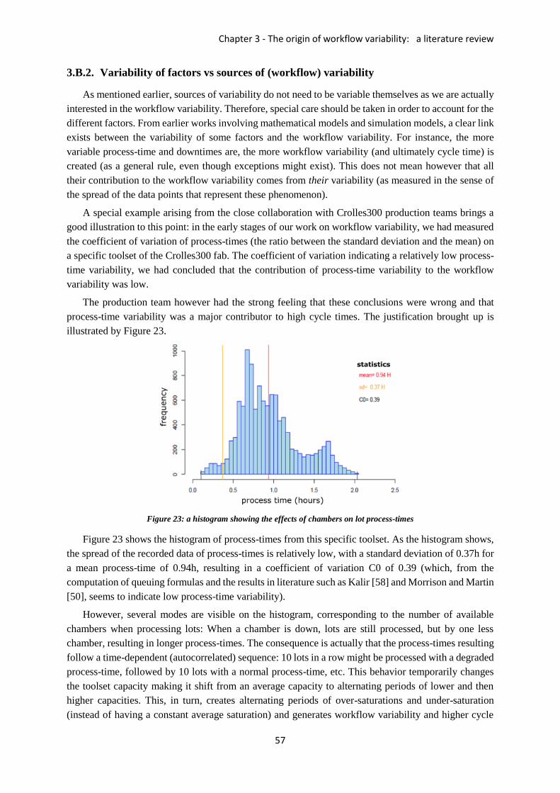
Chapter 3 - The origin of workflow variability: a literature review
57
3.B.2. Variability of factors vs sources of (workflow) variability
As mentioned earlier, sources of variability do not need to be variable themselves as we are actually
interested in the workflow variability. Therefore, special care should be taken in order to account for the
different factors. From earlier works involving mathematical models and simulation models, a clear link
exists between the variability of some factors and the workflow variability. For instance, the more
variable process-time and downtimes are, the more workflow variability (and ultimately cycle time) is
created (as a general rule, even though exceptions might exist). This does not mean however that all
their contribution to the workflow variability comes from their variability (as measured in the sense of
the spread of the data points that represent these phenomenon).
A special example arising from the close collaboration with Crolles300 production teams brings a
good illustration to this point: in the early stages of our work on workflow variability, we had measured
the coefficient of variation of process-times (the ratio between the standard deviation and the mean) on
a specific toolset of the Crolles300 fab. The coefficient of variation indicating a relatively low process-
time variability, we had concluded that the contribution of process-time variability to the workflow
variability was low.
The production team however had the strong feeling that these conclusions were wrong and that
process-time variability was a major contributor to high cycle times. The justification brought up is
illustrated by Figure 23.
Figure 23: a histogram showing the effects of chambers on lot process-times
Figure 23 shows the histogram of process-times from this specific toolset. As the histogram shows,
the spread of the recorded data of process-times is relatively low, with a standard deviation of 0.37h for
a mean process-time of 0.94h, resulting in a coefficient of variation C0 of 0.39 (which, from the
computation of queuing formulas and the results in literature such as Kalir [58] and Morrison and Martin
[50], seems to indicate low process-time variability).
However, several modes are visible on the histogram, corresponding to the number of available
chambers when processing lots: When a chamber is down, lots are still processed, but by one less
chamber, resulting in longer process-times. The consequence is actually that the process-times resulting
follow a time-dependent (autocorrelated) sequence: 10 lots in a row might be processed with a degraded
process-time, followed by 10 lots with a normal process-time, etc. This behavior temporarily changes
the toolset capacity making it shift from an average capacity to alternating periods of lower and then
higher capacities. This, in turn, creates alternating periods of over-saturations and under-saturation
(instead of having a constant average saturation) and generates workflow variability and higher cycle

Part One - What is “variability”?
58
times. This extra variability created by the dependency of the process-times cannot be captured by
measuring variability of the process-times as the spread of the data: if we were to simulate this toolset
with process-times described only by a statistical distribution, we would fail to incorporate this specific
root cause of variability as we would not recreate these alternating periods of longer and shorter cycle
times. The important aspect here is that sources of variability participate to workflow variability in
intricate manners, and, especially in complex manufacturing, special attention should be devoted to
identify what creates workflow variability in the real world.
3.B.3. Concluding our literature review of the sources of variability
With our above discussion, we made clear that sources of variability are sources of workflow
variability. This idea should always be the main driver when studying the impact of different sources of
variability: it is not the source that should be measured, but its consequences. Any measure that we make
on a source of variability should be intended to this purpose.
The coefficient of variation of an event linked to a specific source of variability (for instance
coefficient of variation of process-times) can be a way to explain the contribution of this source to the
workflow variability, it may however be insufficient. As a general rule, the assumptions that build a
reasoning should be stated out loud and investigated as complex manufacturing systems tend, as we will
see in chapter 6, to not play by the simple rules.
From this literature review, we also understand that it is often the combination of factors that result
in high workflow variability. In semiconductor manufacturing, all of the mentioned sources of
variability are part of the everyday life production. We gave in sections 1.A.5 and 1.B.2 short
explanations of why semiconductor manufacturing and especially High Mix Low Volume
semiconductor manufacturing is subject to more workflow variability. With the explanation of this
chapter, we now understand that semiconductor fabs are subject to all of the sources of variability that
we have previously listed, allowing them the title of complex manufacturing. Moreover, as HMLV fabs
have a broader range of products, the product-induced sources of variability are expressed far more,
giving rise to more workflow variability. On top of that, as HMLV have lower volumes for each product,
the structure needs to be adjusted to this kind of production: fewer redundancy per product-level and
therefore higher degree of reentrancy and more complication qualification schemes (with resulting tool
dedications allowing smaller “communication channels” between tools). Another direct consequence of
having more product-levels per tool is that the equipment-specific factors have bigger impacts: more
setups, more incomplete batches, tools subject to more changes and stress from switching between
different recipes and therefore more downtimes and process-time variability… Finally, with higher
reentrancy and more different products in lower volumes, the operational factors get harder to handle:
the smaller volumes per product mean less engineering time per product and therefore more holds, the
numerous different flows and higher reentrancy make it harder to predict the future and therefore harder
to implement maintenance and WIP control strategies, and the dispatching algorithms have to deal with
many more parameters which increases the complexity of their problems.
The work in this chapter and in part One of this manuscript allowed us a better understanding and
an overall picture of what workflow variability is, how it manifests, and what the main root causes are.
With that in mind, the next step is to adjust the production management tools to this new level of
understanding of workflow variability in order to deal as well as possible with the existing level of
workflow variability in manufacturing environments.

Chapter 3 - The origin of workflow variability: a literature review
59
Part Two
II Integrating variability (in production management tools)
Part One of this manuscript was devoted to understanding in-depth what “variability” is, or as we
clarified it in part One, what workflow variability is. We therefore covered this central notion of
workflow variability in all of its aspects: the consequences, the manifestation of workflow variability,
the quantification of it and the identification of its main root causes.
Part Two is aimed at dealing with workflow variability by integrating it in different production
management tools. In order to do so, we will first present in chapter 4 a solution to integrate the
“background consequences” of workflow variability in the projection tool of a manufacturing system.
This solution, developed and implemented at ST Crolles for both fabs under the name Maestro,
effectively allows making projections that are closer from the natural behavior of the system, thus
increasing the accuracy of the projection tool and the efficiency of the downstream actions, resulting in
a better tractability of the manufacturing system.
Integrating variability also means creating models that incorporate all the sources of variability
identified in chapter 3. The first step to do so is to accurately measure the actual performances of
process-clusters, which standard analytical tools such as the OEE [64] are unable to fully do because of
the complex interactions between the numerous sources of variability. Chapter 5 will address this issue
by introducing a new notion: the Concurrent WIP. Along with associated measures, we will propose in
chapter 5 a way to analyze the aggregated response of process-clusters to incoming flows in order to
incorporate the effects of all sources of variability and get a better picture of the performance of process-
clusters.
The second step to better incorporate variability into different models is to better understand the
underlying mechanisms which create workflow variability, one of which we believe is effects of
dependencies. We will therefore investigate in chapter 6 the effects of dependencies on downtimes,
process-times and arrivals. We will propose a method to do so by running simulations using actual shop
floor data, and will show through our results that dependencies can actually be responsible for a far
bigger amount of workflow variability than previously expected, and that developing tools in this
direction could greatly improve the integration and reduction of workflow variability.
Chapter 5 shows work presented at the 2016 International Conference on Modeling, Optimization
& Simulation (MOSIM) [3] and submitted to the journal of IEEE Transactions on Automation, Science
and Engineering (TASE), and the results of chapter 6 were partly presented at the 2017 International
Conference on Industrial Engineering and Systems Management (IESM).


Chapter 4 - Maestro: integrating background variability
61
Chapter 4
4. Maestro:
integrating background variability
Workflow variability has consequences in terms of added cycle time and tractability, as we have
explained in chapter 1. However, as a part of the sources of variability is stable (such as equipment-
specific or structural factors, see chapter 3), a part of the consequences is predictable. More precisely,
the time spent by lots to cross different sections of the manufacturing system is not totally unpredictable,
it is the result of many interactions between all the different sources of variability, it is in other words
the background consequence of workflow variability.
Chapter 4 presents the different aspects, tools and methods, which allow integrating this background
variability into the projection tool. We first discuss (4.A) the specificities of making WIP projections
based on cycle time models (which is the type of projection used at ST Microelectronics), and show
how the quality of a cycle time model greatly impacts the projection as well as the actions based upon
these projections. We then show how historical data can be used to build a cycle time model, using a
multi-layer model to overpass a “scale dilemma” we point out, which would make simple bottom-up
approaches unfit. As HMLV manufacturing systems undergo changes in product-mix and loading, one
might think that using historical data would be of little use to make projections. We however show that
the structure of HMLV manufacturing systems actually make the background variability shift rather than
break, and that using the correct algorithms can allow to greatly improve cycle time models for short
and mid-term projections.
The problem that is presented in this chapter comes from a real-world situation faced by the
Industrial Engineering team at ST Microelectronics Crolles. The projection software, Opera, previously
used to project the WIP based on a cycle time model that did not take into account the effects of
workflow variability on cycle time and the actions that depend on this projection (all matters of resource
allocation, delivery targets, and production objectives) suffered from this inaccuracy. The results
presented in this chapter were implemented and industrialized in a software, Maestro, which now
computes the cycle time models for the entire WIP of the two C200 and C300 fabs, thus giving to Opera
the tempo to follow for its WIP projections.
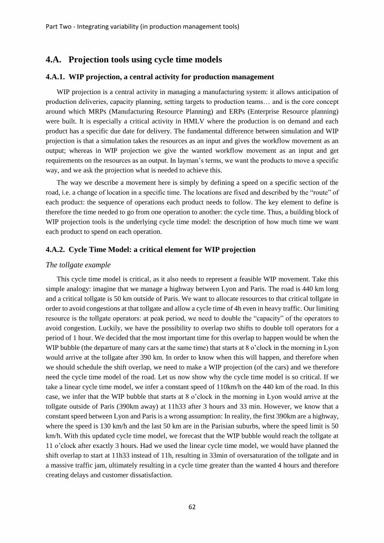
Part Two - Integrating variability (in production management tools)
62
4.A. Projection tools using cycle time models
4.A.1. WIP projection, a central activity for production management
WIP projection is a central activity in managing a manufacturing system: it allows anticipation of
production deliveries, capacity planning, setting targets to production teams… and is the core concept
around which MRPs (Manufacturing Resource Planning) and ERPs (Enterprise Resource planning)
were built. It is especially a critical activity in HMLV where the production is on demand and each
product has a specific due date for delivery. The fundamental difference between simulation and WIP
projection is that a simulation takes the resources as an input and gives the workflow movement as an
output; whereas in WIP projection we give the wanted workflow movement as an input and get
requirements on the resources as an output. In layman’s terms, we want the products to move a specific
way, and we ask the projection what is needed to achieve this.
The way we describe a movement here is simply by defining a speed on a specific section of the
road, i.e. a change of location in a specific time. The locations are fixed and described by the “route” of
each product: the sequence of operations each product needs to follow. The key element to define is
therefore the time needed to go from one operation to another: the cycle time. Thus, a building block of
WIP projection tools is the underlying cycle time model: the description of how much time we want
each product to spend on each operation.
4.A.2. Cycle Time Model: a critical element for WIP projection
The tollgate example
This cycle time model is critical, as it also needs to represent a feasible WIP movement. Take this
simple analogy: imagine that we manage a highway between Lyon and Paris. The road is 440 km long
and a critical tollgate is 50 km outside of Paris. We want to allocate resources to that critical tollgate in
order to avoid congestions at that tollgate and allow a cycle time of 4h even in heavy traffic. Our limiting
resource is the tollgate operators: at peak period, we need to double the “capacity” of the operators to
avoid congestion. Luckily, we have the possibility to overlap two shifts to double toll operators for a
period of 1 hour. We decided that the most important time for this overlap to happen would be when the
WIP bubble (the departure of many cars at the same time) that starts at 8 o’clock in the morning in Lyon
would arrive at the tollgate after 390 km. In order to know when this will happen, and therefore when
we should schedule the shift overlap, we need to make a WIP projection (of the cars) and we therefore
need the cycle time model of the road. Let us now show why the cycle time model is so critical. If we
take a linear cycle time model, we infer a constant speed of 110km/h on the 440 km of the road. In this
case, we infer that the WIP bubble that starts at 8 o’clock in the morning in Lyon would arrive at the
tollgate outside of Paris (390km away) at 11h33 after 3 hours and 33 min. However, we know that a
constant speed between Lyon and Paris is a wrong assumption: In reality, the first 390km are a highway,
where the speed is 130 km/h and the last 50 km are in the Parisian suburbs, where the speed limit is 50
km/h. With this updated cycle time model, we forecast that the WIP bubble would reach the tollgate at
11 o’clock after exactly 3 hours. Had we used the linear cycle time model, we would have planned the
shift overlap to start at 11h33 instead of 11h, resulting in 33min of oversaturation of the tollgate and in
a massive traffic jam, ultimately resulting in a cycle time greater than the wanted 4 hours and therefore
creating delays and customer dissatisfaction.
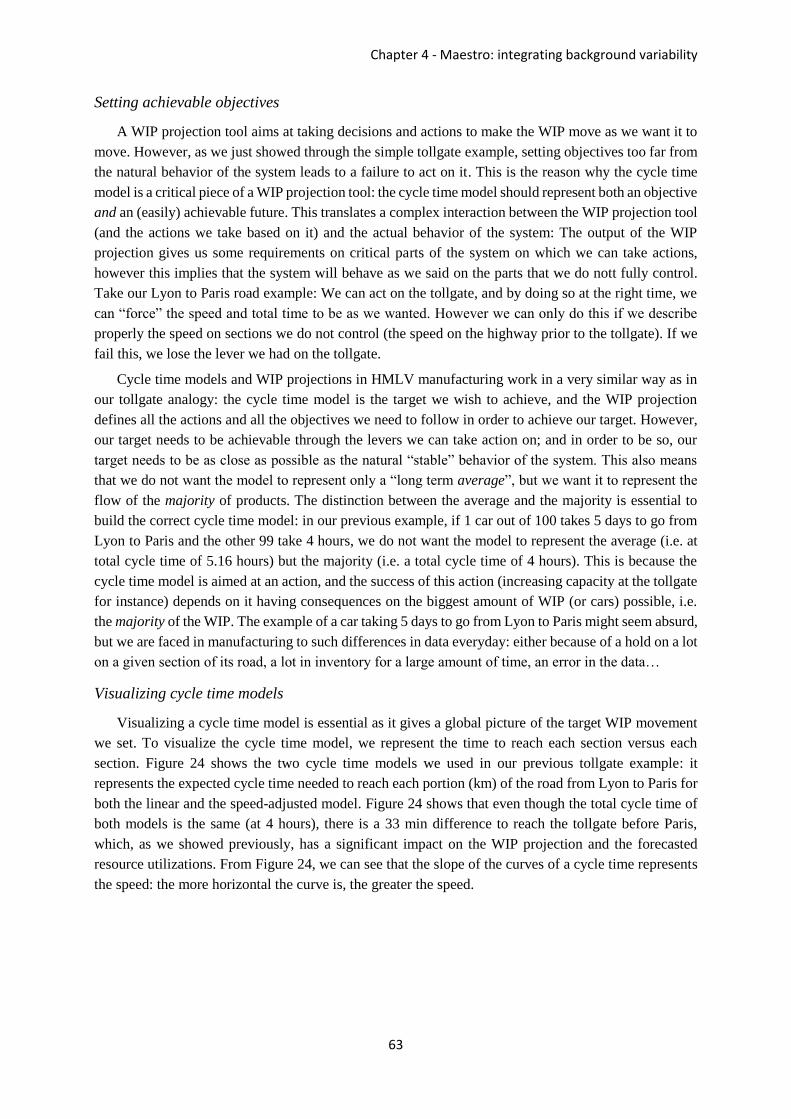
Chapter 4 - Maestro: integrating background variability
63
Setting achievable objectives
A WIP projection tool aims at taking decisions and actions to make the WIP move as we want it to
move. However, as we just showed through the simple tollgate example, setting objectives too far from
the natural behavior of the system leads to a failure to act on it. This is the reason why the cycle time
model is a critical piece of a WIP projection tool: the cycle time model should represent both an objective
and an (easily) achievable future. This translates a complex interaction between the WIP projection tool
(and the actions we take based on it) and the actual behavior of the system: The output of the WIP
projection gives us some requirements on critical parts of the system on which we can take actions,
however this implies that the system will behave as we said on the parts that we do nott fully control.
Take our Lyon to Paris road example: We can act on the tollgate, and by doing so at the right time, we
can “force” the speed and total time to be as we wanted. However we can only do this if we describe
properly the speed on sections we do not control (the speed on the highway prior to the tollgate). If we
fail this, we lose the lever we had on the tollgate.
Cycle time models and WIP projections in HMLV manufacturing work in a very similar way as in
our tollgate analogy: the cycle time model is the target we wish to achieve, and the WIP projection
defines all the actions and all the objectives we need to follow in order to achieve our target. However,
our target needs to be achievable through the levers we can take action on; and in order to be so, our
target needs to be as close as possible as the natural “stable” behavior of the system. This also means
that we do not want the model to represent only a “long term average”, but we want it to represent the
flow of the majority of products. The distinction between the average and the majority is essential to
build the correct cycle time model: in our previous example, if 1 car out of 100 takes 5 days to go from
Lyon to Paris and the other 99 take 4 hours, we do not want the model to represent the average (i.e. at
total cycle time of 5.16 hours) but the majority (i.e. a total cycle time of 4 hours). This is because the
cycle time model is aimed at an action, and the success of this action (increasing capacity at the tollgate
for instance) depends on it having consequences on the biggest amount of WIP (or cars) possible, i.e.
the majority of the WIP. The example of a car taking 5 days to go from Lyon to Paris might seem absurd,
but we are faced in manufacturing to such differences in data everyday: either because of a hold on a lot
on a given section of its road, a lot in inventory for a large amount of time, an error in the data…
Visualizing cycle time models
Visualizing a cycle time model is essential as it gives a global picture of the target WIP movement
we set. To visualize the cycle time model, we represent the time to reach each section versus each
section. Figure 24 shows the two cycle time models we used in our previous tollgate example: it
represents the expected cycle time needed to reach each portion (km) of the road from Lyon to Paris for
both the linear and the speed-adjusted model. Figure 24 shows that even though the total cycle time of
both models is the same (at 4 hours), there is a 33 min difference to reach the tollgate before Paris,
which, as we showed previously, has a significant impact on the WIP projection and the forecasted
resource utilizations. From Figure 24, we can see that the slope of the curves of a cycle time represents
the speed: the more horizontal the curve is, the greater the speed.
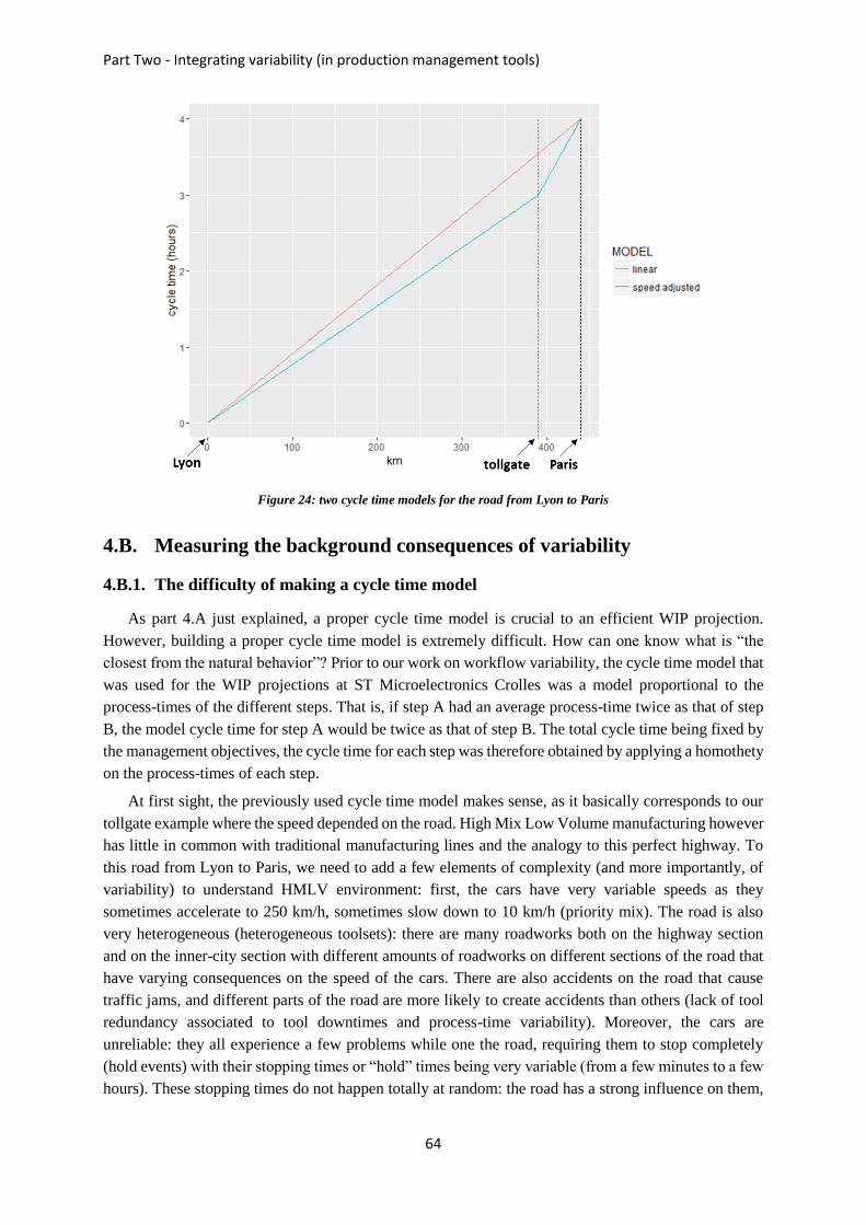
Part Two - Integrating variability (in production management tools)
64
Figure 24: two cycle time models for the road from Lyon to Paris
4.B. Measuring the background consequences of variability
4.B.1. The difficulty of making a cycle time model
As part 4.A just explained, a proper cycle time model is crucial to an efficient WIP projection.
However, building a proper cycle time model is extremely difficult. How can one know what is “the
closest from the natural behavior”? Prior to our work on workflow variability, the cycle time model that
was used for the WIP projections at ST Microelectronics Crolles was a model proportional to the
process-times of the different steps. That is, if step A had an average process-time twice as that of step
B, the model cycle time for step A would be twice as that of step B. The total cycle time being fixed by
the management objectives, the cycle time for each step was therefore obtained by applying a homothety
on the process-times of each step.
At first sight, the previously used cycle time model makes sense, as it basically corresponds to our
tollgate example where the speed depended on the road. High Mix Low Volume manufacturing however
has little in common with traditional manufacturing lines and the analogy to this perfect highway. To
this road from Lyon to Paris, we need to add a few elements of complexity (and more importantly, of
variability) to understand HMLV environment: first, the cars have very variable speeds as they
sometimes accelerate to 250 km/h, sometimes slow down to 10 km/h (priority mix). The road is also
very heterogeneous (heterogeneous toolsets): there are many roadworks both on the highway section
and on the inner-city section with different amounts of roadworks on different sections of the road that
have varying consequences on the speed of the cars. There are also accidents on the road that cause
traffic jams, and different parts of the road are more likely to create accidents than others (lack of tool
redundancy associated to tool downtimes and process-time variability). Moreover, the cars are
unreliable: they all experience a few problems while one the road, requiring them to stop completely
(hold events) with their stopping times or “hold” times being very variable (from a few minutes to a few
hours). These stopping times do not happen totally at random: the road has a strong influence on them,
Chapter 4 - Maestro: integrating background variability
65
with humid parts of the road creating more failures in the cars (hold times linked to time constraints).
This new, extremely variable road is a better analogy to the complexity we face in HMVL production.
From this example, and the explanations on workflow variability that we gave in part One, we see
that the type of the road (the process-time) has only a small influence on the actual cycle times: in our
road analogy, we can easily find a inner-city portion of road with a speed higher that a highway portion
of road… The workflow variability affects the system too much for this simple cycle time model to
work.
4.B.2. The background consequence of variability
Consequences of variability: an order in chaos
Being able to build a cycle time model and therefore make WIP projections in this environment may
seem counterintuitive as one consequence of variability, as our road analogy pointed out, is the
uncertainty it adds to the flow of the products. Indeed, it is almost impossible in a HMLV context to
forecast with precision the movement of any lot on a small scale: the combined effects of variability add
so much randomness that we are actually certain that we cannot predict exactly the movement of any
lot.
However, we classified in chapter 3 different sources of variability and defined some as “structural”
and others as “equipment specific”. These sources of variability have a strong inertia: it takes time to
add tools or to qualify new tools, batch tools will keep making batches in the future, the sequence of
operations (and therefore of machines) basically stay the same… What this means is that even though
the variability is high and the flow is partly unpredictable, a part of the sources of variability stays the
same and therefore a part of the consequences as well. This is what we call the “background
consequences” of variability: even though everything is extremely variable, the consequences are
variable around a certain value. In our previous analogy, updating the road to the new description, there
will still be a given time most cars take to travel from Lyon to Paris… Moreover, there would also be
distinctive speeds on the different portions of the road: some portions would be slower, some portions
would be faster, and some portions would be in the average… A good cycle time model therefore needs
to incorporate these relative differences in speed in order to be as close as possible to the “natural
behavior” of the system.
Using historical data to build the cycle time model
Different solutions could be investigated to integrate this effect of workflow variability (the
background macro consequence on the relative speed of lots). One solution would be to use queueing
theory to estimate cycle time at the different steps of the roads. However, as we explained in chapter 1,
queuing theory only integrates few sources of variability under specific conditions. When we compare
this to the extended list of sources of variability presented in chapter 3, and all the possible interactions
between these responsible for workflow variability, we can doubt beforehand of the results that would
be obtained should we go in this direction.
The solution that we propose to this problem is “simply” to use historical data to build our cycle
time model. Indeed, as the strong inertia of the structural and equipment-specific sources of variability
create a somewhat stable background response, this consequence is in theory measurable, and the near
future should in theory be close to the near past.
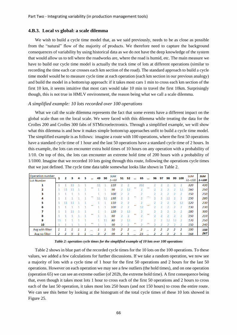
Part Two - Integrating variability (in production management tools)
66
4.B.3. Local vs global: a scale dilemma
We wish to build a cycle time model that, as we said previously, needs to be as close as possible
from the “natural” flow of the majority of products. We therefore need to capture the background
consequences of variability by using historical data as we do not have the deep knowledge of the system
that would allow us to tell where the roadworks are, where the road is humid, etc. The main measure we
have to build our cycle time model is actually the track time of lots at different operations (similar to
recording the time each car crosses each km section of the road). The standard approach to build a cycle
time model would be to measure cycle time at each operation (each km section in our previous analogy)
and build the model in a bottom/up approach: if it takes most cars 1 min to cross each km section of the
first 10 km, it seems intuitive that most cars would take 10 min to travel the first 10km. Surprisingly
though, this is not true in HMLV environment, the reason being what we call a scale dilemma.
A simplified example: 10 lots recorded over 100 operations
What we call the scale dilemma represents the fact that some events have a different impact on the
global scale than on the local scale. We were faced with this dilemma while treating the data for the
Crolles 200 and Crolles 300 fabs of STMicroelectronics. Through a simplified example, we will show
what this dilemma is and how it makes simple bottom/up approaches unfit to build a cycle time model.
The simplified example is as follows: imagine a route with 100 operations, where the first 50 operations
have a standard cycle time of 1 hour and the last 50 operations have a standard cycle time of 2 hours. In
this example, the lots can encounter extra hold times of 10 hours on any operation with a probability of
1/10. On top of this, the lots can encounter an extreme hold time of 200 hours with a probability of
1/1000. Imagine that we recorded 10 lots going through this route, following the operations cycle times
that we just defined. The cycle time data table somewhat looks like shown in Table 2.
Table 2: operation cycle times for the simplified example of 10 lots over 100 operations
Table 2 shows in blue part of the recorded cycle times for the 10 lots on the 100 operations. To these
values, we added a few calculations for further discussions. If we take a random operation, we now see
a majority of lots with a cycle time of 1 hour for the first 50 operations and 2 hours for the last 50
operations. However on each operation we may see a few outliers (the hold times), and on one operation
(operation 65) we can see an extreme outlier (of 202h, the extreme hold time). A first consequence being
that, even though it takes most lots 1 hour to cross each of the first 50 operations and 2 hours to cross
each of the last 50 operation, it takes most lots 250 hours (and not 150 hours) to cross the entire route.
We can see this better by looking at the histogram of the total cycle times of these 10 lots showed in
Figure 25.
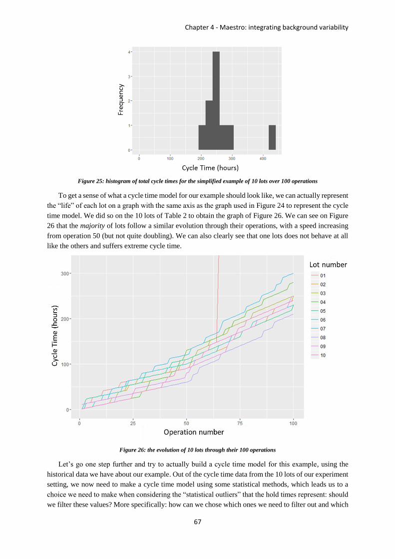
Chapter 4 - Maestro: integrating background variability
67
Figure 25: histogram of total cycle times for the simplified example of 10 lots over 100 operations
To get a sense of what a cycle time model for our example should look like, we can actually represent
the “life” of each lot on a graph with the same axis as the graph used in Figure 24 to represent the cycle
time model. We did so on the 10 lots of Table 2 to obtain the graph of Figure 26. We can see on Figure
26 that the majority of lots follow a similar evolution through their operations, with a speed increasing
from operation 50 (but not quite doubling). We can also clearly see that one lots does not behave at all
like the others and suffers extreme cycle time.
Figure 26: the evolution of 10 lots through their 100 operations
Let’s go one step further and try to actually build a cycle time model for this example, using the
historical data we have about our example. Out of the cycle time data from the 10 lots of our experiment
setting, we now need to make a cycle time model using some statistical methods, which leads us to a
choice we need to make when considering the “statistical outliers” that the hold times represent: should
we filter these values? More specifically: how can we chose which ones we need to filter out and which
Part Two - Integrating variability (in production management tools)
68
ones we need to keep in? In order to locally represent the movement of the majority, we should filter
the outliers (since most lots have a cycle time of 1h in the first 50 operations and of 2h in the last 50
operations). However if we do so, we become terrible at predicting the flow of the majority of products
on the macroscopic scale: As Figure 25 and Figure 26 show, the majority of lots take 250 hours to
complete their route, and by filtering locally, we would make a model that has a total cycle time of 150
hours (as we can see in the “average with filter” row of Table 2). If we do not filter anything however
(and make an average cycle time for each operation), we would locally have a pretty bad model (since,
for instance, we would put 3 hours at operation 2, a value that does not represent the movement of
anyone) and also have an inaccurate global cycle time model (As shown in Table 2, we would get a total
cycle time value of 269 hours, when most lots actually take around 250 hours).
This problem, which we presented here in a simplified manner, is what we call the scale dilemma:
it seems impossible to compute from the data a model that represents the movement of the majority of
products both on the local and on the global scale. The reason we can actually not make a good cycle
time model using only local information computed in a partitioned way (i.e. measuring statistics on each
operation separately) is that the hold events from our example have different consequences on different
scales. Locally, all hold events are outliers, as on the scale of operations, they do not represent the
behavior of the majority. Globally however, some hold events actually affect all lots in a similar way
and they then do represent the behavior of the majority, as we can understand by looking at the flow
movement in Figure 26.
Figure 25 also shows why we would get a bad global model by computing the average operation
cycle time with no filter: one lot has a cycle time far different than the rest, because it was affected by
an extreme hold that does not represent the majority on the global scale. What we start understanding
here is that each scale needs to tell us which information needs to be kept for its own level. Think of it
this way: for each operation, the high cycle times coming from holds (+10 hours) or from the extreme
holds (+200 hours) are both outliers, and there is absolutely no way of telling which should be considered
or not for the model if we only stick to these local measures. The only way to tell that some are not
outliers for what we measure is by looking at the global picture because it is at this scale that we define
what is normal or not. This is the heart of what we call the scale dilemma. We get contradictive
information from different scales (e.g. the answer to the question “are hold events outliers?”) but we
still wish to make a single model representative of all scales.
Bonus problem: sample size
For our use of the cycle time model, we want it to be accurate on the global scale, so we obviously
need it to be slightly off locally. However, we still want to reduce this offset as much as we can. This is
where another problem of scale comes: the sampling size. Indeed, even if we remove the global outliers
(the extreme hold event), the estimator of the mean has a huge uncertainty for a sampling size of 10: if
we take the average per operation, we would get stricktly different times for operations that we know
are actually the same (the last 50 operations for instance). However, this problem of sampling size is the
reality we face in High Mix Low Volume production: the amount of data per aggregation level is scarce.
In order to solve this sampling size problem, let us first build a cycle time model for our example
based on the statistical parameters, which we can do in this case since we already know the statistical
parameters and do not actually need to estimate them. As we explained previously, the outlier here is
defined by the impact on the global scale and only the extreme hold here is considered as an outlier.
Once we removed the extreme hold value, we are left for each operation with standard cycle times as
well as holds that occur with a probability of 1/10. Therefore, the mean cycle time for each operation is

Chapter 4 - Maestro: integrating background variability
69
the standard cycle time of the operation + 1h (10h with probability 1/10). Our cycle time model based
on the statistical parameters is therefore 2 hours for each of the first 50 operations, and 3 hours for each
of the last 50 operations (for a total cycle time of 250 hours). We would reach these values if we had an
“infinite” amount of points and no sampling size problem. We now need a method that allows us to
come close to this result by only using the data of our 10 lots.
4.B.4. A multi-layer model solution
The solution we propose to the problem of scale and sampling size is to measure information on
each of the important scale, and to recombine them to have a homogeneous shift from one scale to
another, in what we call a multi-layer model. For instance, if we only care about the local cycle time and
the total cycle time (but no timescale in between), we could do a double-layer model. We first measure
all local cycle times by filtering all local outliers, we then measure the total cycle times and filter all
global outliers, and we finally stretch all local values by applying a homothety, so that the sum of local
cycle times adds to the total cycle time we decided. With this double layer model on our example, we
would have cycle times of 1.66 h for the first 50 operations, and 3.33 for the last 50 operations (by
starting at 1h for the first 50 operations and 2h for the last 50 operations, and apply the homothety to
stretch these values until the sum equals 250h). It would seem that we have an acceptable model. Indeed,
with these values, we get cycle times that are twice as long on the last 50 operations than the first 50
operations (which corresponds to the ratio of standard cycle time as we can see in Table 2) and we have
a total cycle time that adds up to 250 hours, which indeed corresponds to the majority of lots.
However, by using a double layer model, we are off on the medium scale: the true time it takes most
lots to complete the first 50 operations is around 100 hours (as we can see from the corresponding
column in Table 2, as well as from Figure 26), when the double-layer model would give a time of 83
hours… As is, this cycle time model would therefore fail to accurately describe the flow of products on
the medium scale. We can however increase the precision by adding another layer to make a triple-layer
model: we divide the road into several sections, and measure the cycle time for each section (removing
outliers on this timescale if we found some). We then proceed as before with two homothety as we show
in Figure 27.
Figure 27: applying a double homothety to get a triple layer cycle time model
We see in Figure 27 that in the case of a triple layer, the bottom layer values (at the operation level
for our example) are multiplied twice to get their final values. They get a first multiplication for their
sum to add to the middle layer values, and a second for the middle values to add to the top layer value.
In our case, the top layer corresponds to the total cycle times, the middle layer correspond to the sections
we divide the road in, and the bottom layer corresponds to the operations.
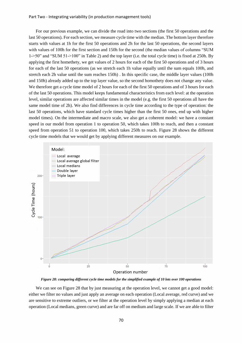
Part Two - Integrating variability (in production management tools)
70
For our previous example, we can divide the road into two sections (the first 50 operations and the
last 50 operations). For each section, we measure cycle time with the median. The bottom layer therefore
starts with values at 1h for the first 50 operations and 2h for the last 50 operations, the second layers
with values of 100h for the first section and 150h for the second (the median values of columns “SUM
1->50” and “SUM 51->100” in Table 2) and the top layer (i.e. the total cycle time) is fixed at 250h. By
applying the first homethety, we get values of 2 hours for each of the first 50 operations and of 3 hours
for each of the last 50 operations (as we stretch each 1h value equally until the sum equals 100h, and
stretch each 2h value until the sum reaches 150h) . In this specific case, the middle layer values (100h
and 150h) already added up to the top layer value, so the second homothety does not change any value.
We therefore get a cycle time model of 2 hours for each of the first 50 operations and of 3 hours for each
of the last 50 operations. This model keeps fundamental characteristics from each level: at the operation
level, similar operations are affected similar times in the model (e.g. the first 50 operations all have the
same model time of 2h). We also find differences in cycle time according to the type of operation: the
last 50 operations, which have standard cycle times higher than the first 50 ones, end up with higher
model times). On the intermediate and macro scale, we also get a coherent model: we have a constant
speed in our model from operation 1 to operation 50, which takes 100h to reach, and then a constant
speed from operation 51 to operation 100, which takes 250h to reach. Figure 28 shows the different
cycle time models that we would get by applying different measures on our example.
Figure 28: comparing different cycle time models for the simplified example of 10 lots over 100 operations
We can see on Figure 28 that by just measuring at the operation level, we cannot get a good model:
either we filter no values and just apply an average on each operation (Local average, red curve) and we
are sensitive to extreme outliers, or we filter at the operation level by simply applying a median at each
operation (Local medians, green curve) and are far off on medium and large scale. If we are able to filter
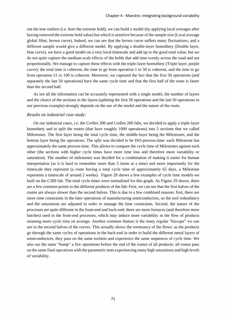
Chapter 4 - Maestro: integrating background variability
71
out the true outliers (i.e. here the extreme hold), we can build a model (by applying local averages after
having removed the extreme hold value) but which is sensitive because of the sample size (Local average
global filter, brown curve). Indeed, we can see that the brown curve suffers many fluctuations, and a
different sample would give a different model. By applying a double-layer homothety (Double layer,
blue curve), we have a good model on a very local timescale and add up to the good total value, but we
do not quite capture the medium scale effects of the holds that add time evenly across the road and not
proportionally. We manage to capture these effects with the triple-layer homothety (Triple layer, purple
curve): the total time is coherent, the time to go from operation 1 to 50 is coherent, and the time to go
from operation 51 to 100 is coherent. Moreover, we captured the fact that the first 50 operations (and
separately the last 50 operations) have the same cycle time and that the first half of the route is faster
than the second half.
As not all the information can be accurately represented with a single model, the number of layers
and the choice of the sections in the layers (splitting the first 50 operations and the last 50 operations in
our previous example) strongly depends on the use of the model and the nature of the route.
Results on industrial case study:
On our industrial cases, i.e. the Crolles 300 and Crolles 200 fabs, we decided to apply a triple-layer
homothety and to split the routes (that have roughly 1000 operations) into 5 sections that we called
Milestones. The first layer being the total cycle time, the middle-layer being the Milestones, and the
bottom layer being the operations. The split was decided to be ISO-process-time: each Milestone has
approximately the same process-time. This allows to compare the cycle time of Milestones against each
other (the sections with higher cycle times have more time loss and therefore more variability or
saturation). The number of milestones was decided for a combination of making it easier for human
interpretation (as it is hard to remember more than 5 items at a time) and more importantly for the
timescale they represent (a route having a total cycle time of approximately 65 days, a Milestone
represents a timescale of around 2 weeks). Figure 29 shows a few examples of cycle time models we
built on the C300 fab. The total cycle times were normalized for this graph. As Figure 29 shows, there
are a few common points to the different products of the fab: First, we can see that the first halves of the
routes are always slower than the second halves. This is due to a few combined reasons: first, there are
more time constraints in the later operations of manufacturing semiconductors, so the tool redundancy
and the saturations are adjusted in order to manage the time constraints. Second, the nature of the
processes are quite different in the front-end and back-end: there are more furnaces (and therefore more
batches) used in the front-end processes, which may induce more variability in the flow of products
meaning more cycle time on average. Another common feature is the many regular “hiccups” we can
see in the second halves of the curves. This actually shows the reentrancy of the flows: as the products
go through the same cycles of operations in the back-end in order to build the different metal layers of
semiconductors, they pass on the same toolsets and experience the same sequences of cycle time. We
also see the same “bump” a few operations before the end of the routes of all products: all routes pass
on the same final operations with the parametric tests experiencing many high saturations and high levels
of variability.
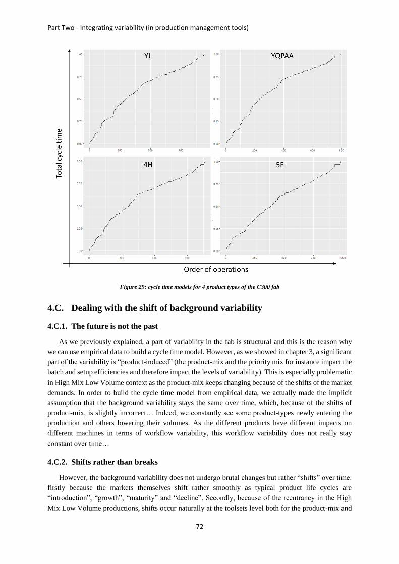
Part Two - Integrating variability (in production management tools)
72
Figure 29: cycle time models for 4 product types of the C300 fab
4.C. Dealing with the shift of background variability
4.C.1. The future is not the past
As we previously explained, a part of variability in the fab is structural and this is the reason why
we can use empirical data to build a cycle time model. However, as we showed in chapter 3, a significant
part of the variability is “product-induced” (the product-mix and the priority mix for instance impact the
batch and setup efficiencies and therefore impact the levels of variability). This is especially problematic
in High Mix Low Volume context as the product-mix keeps changing because of the shifts of the market
demands. In order to build the cycle time model from empirical data, we actually made the implicit
assumption that the background variability stays the same over time, which, because of the shifts of
product-mix, is slightly incorrect… Indeed, we constantly see some product-types newly entering the
production and others lowering their volumes. As the different products have different impacts on
different machines in terms of workflow variability, this workflow variability does not really stay
constant over time…
4.C.2. Shifts rather than breaks
However, the background variability does not undergo brutal changes but rather “shifts” over time:
firstly because the markets themselves shift rather smoothly as typical product life cycles are
“introduction”, “growth”, “maturity” and “decline”. Secondly, because of the reentrancy in the High
Mix Low Volume productions, shifts occur naturally at the toolsets level both for the product-mix and

Chapter 4 - Maestro: integrating background variability
73
for the saturations. Indeed, take the example of an initially empty fab that brutally starts the flow of
products and starts 100 lots per week. Imagine a toolset T with a reentrancy of 10 (the products come
back at this toolset 10 times) where it takes one week for the products to come back to this toolset. The
first week, 100 lots (the ones we just started) will go through toolset T. The second week, 100 newly
started lots will go through T, as well as the first 100 lots that would reenter for the first time on T.
Therefore, the second week, 200 lots in total will go through the toolset T. This shift will increase
linearly until reaching stability after 10 weeks at 1000 lots per week going through T. For the same
reasons, the same shift applies to the product-mix. We can therefore make the reasonable assumption
that the background variability changes over time, but changes somewhat smoothly with a change rate
of several weeks corresponding to the reentrancy period. This assumption is strengthened by the
industrial data, an example being shown by Figure 30.
Figure 30: evolution of lot cycle times for a given product and a given Milestone of the C200 fab
Figure 30 shows the Milestone cycle time for a specific product type in the C200 fab. It displays for
each lot the cycle time it took to cross this Milestone against the date it exited the Milestone. This
illustrates the shift of background variability: over a period of 6 months, the cycle time to cross this
section for this product gradually increased from 11 days to 14 days.
The consequence of this shift is that we cannot simply use an average or a median on the past to
measure cycle times for each aggregation level of our cycle time model (as we did in the previous simple
example). We can, however, use the information from the past to forecast, for each aggregation level,
the cycle time the most likely to happen in the near future. Simply put, we need a way to incorporate the
shift of variability in our cycle time model.
4.C.3. Holt-Winter smoothing: Measuring background variability changes
We want to apply our triple-layer model in a way that allows integrating the shift of variability.
Therefore, for each aggregation level of our triple-layer model, we do not want to compute a simple
median on the past but actually make a prediction for the future. Furthermore, since all products interact
with each other (in any HMLV production), the shift of variability is time-based (i.e. it does not depend
on the number of points but on the time): we therefore need a method that capture changes over time
Part Two - Integrating variability (in production management tools)
74
without being influenced too much by the number of points. Indeed, the different products have very
different volumes and the number of points per product varies enormously. This means first
transforming the raw industrial data into a homogeneous time-series. To do so, we can simply aggregate
(for each aggregation level of our triple-layer model) the data of each week by measuring the median
for each period.
Once we have a homogeneous time-series, there are many existing methods in the literature to
forecast the next point of the time series. We chose to apply a double exponential smoothing algorithm,
also known as Holt-Winters (HW) algorithm, as it is a popular technique to provide short-term forecasts
for time series (e.g., [65]). HW algorithm is an iterative algorithm that uses linear combinations of the
previously forecasted value and new observed value to build the new forecasted value. Its strength is to
capture both the trend and the slope in order to make a prediction. For illustration, let us apply the HW
algorithm to the time series we discussed previously (the medians per period). Let us call 𝑀𝑒𝑑𝑖𝑎𝑛𝑇 the
median we measured for period T. As HW algorithm is an iterative algorithm, let 𝐶�̂�𝑇|𝑇−1 be the
forecasted cycle time value for period T that was computed at period T-1. The idea of HW algorithm is
that the forecasted value for period T+1 (𝐶�̂�𝑇+1|𝑇) is the sum of two time series at period T. These two
time series are the trend �̂�𝑇 and the slope �̂�𝑇, and are themselves iteratively estimated by an average of
the last observation 𝑀𝑒𝑑𝑖𝑎𝑛𝑇 and the last predictions, weighted by two parameters λ1 and λ2 as shown
by equations (4) to (6).
�̂�𝑇 = λ1 × 𝑀𝑒𝑑𝑖𝑎𝑛𝑇 + (1 − λ1) × 𝐶�̂�𝑇|𝑇−1 (4)
�̂�𝑇 = λ2 × (�̂�𝑇 − �̂�𝑇−1) + (1 − λ2) × �̂�𝑇−1 (5)
𝐶�̂�𝑇+1|𝑇 = �̂�𝑇 + �̂�𝑇 (6)
The values of the two parameters λ1 and λ2 can either be estimated by minimizing a criterion (the
forecast error for example), or by tuning them to represent a given timescale. In our industrial case, we
chose to set the values in order for the series to represent a timescale: it was decided that the events that
happened more than 3 months ago should not influence the value of the cycle time model.
Mathematically, we translated that by “starting from 0, it takes 3 months to reach 99% of the actual
value in the case where the time series is a constant”. Since each point of the time series represents 1
week, we set the constants λ1 and λ2 so that after 12 iterations, 𝐶�̂�𝑇+1 reaches 99% of 𝑀𝑒𝑑𝑖𝑎𝑛𝑇 when
𝑀𝑒𝑑𝑖𝑎𝑛𝑇 follows a constant. This therefore led us to set the constants to λ1= λ2=0.24.
As this is an iterative method, there needs to be a starting point or an initialization phase. Several
initialization methods exist in the literature [66], one of them being to simply take a median or an average
for �̂�𝑇 and 𝑀𝑒𝑑𝑖𝑎𝑛𝑇 and take an initial slope �̂�𝑇 equal to 0. If the available historical data is big enough
(meaning more than 12 historical medians), this method is sufficient. The performance will however
start degrading if less data is available, which can actually be the case for newly started products for
instance, which do not have any tracks recorded. For these products, we would want our model to give
best performances as soon as possible.
In order to reduce the amount of data needed for a satisfactory initialization, we applied a
“backforecast initialization” [66]. This consists of two phases: we first apply a normal initialization as
we previously explained (computing a median on all data-points for �̂�𝑇 and 𝑀𝑒𝑑𝑖𝑎𝑛𝑇, and setting the
slope �̂�𝑇 to 0); we then apply our entire algorithm (computing medians and HW algorithm) on the
reverse data: instead of reading the time-series left-to-right, we read the time series right-to-left. When
the last week of the backforecast phase is reached, the values we get is a “forecast” of the three time
series (�̂�𝑇, �̂�𝑇, and 𝐶�̂�𝑇) read right-to-left, which we can call �̂�0, �̂�0, and 𝐶�̂�0. The central values �̂�0 and
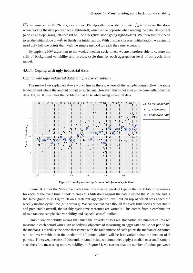
Chapter 4 - Maestro: integrating background variability
75
𝐶�̂�0 are now set as the “best guesses” our HW algorithm was able to make. �̂�0 is however the slope
when reading the data points from right-to-left, which is the opposite when reading the data left-to-right
(a positive slope going left-to-right will be a negative slope going right-to-left). We therefore just need
to set the initial slope to −�̂�0 to finish our initialization. With this backforecast initialization, we actually
need only half the points than with the simple method to reach the same accuracy.
By applying HW algorithm to the weekly median cycle times, we are therefore able to capture the
shift of background variability and forecast cycle time for each aggregation level of our cycle time
model.
4.C.4. Coping with ugly industrial data
Coping with ugly industrial data: sample size variability
The method we explained above works fine in theory, where all the sample points follow the same
tendency and where the amount of data is sufficient. However, this is not always the case with industrial
data. Figure 31 illustrates the problems that arise when using industrial data.
Figure 31: weekly median cycle times built from lot cycle times
Figure 31 shows the Milestone cycle time for a specific product type in the C200 fab. It represents
for each lot the cycle time it took to cross this Milestone against the date it exited the Milestone and is
the same graph as in Figure 30 on a different aggregation level, but on top of which was added the
weekly median cycle time (blue crosses). We can see that even though the cycle time seems rather stable
and predictable overall, the weekly cycle time measures are variable. This comes from a combination
of two factors: sample size variability and “special cause” outliers.
Sample size variability means that since the arrivals of lots are stochastic, the number of lots we
measure in each period varies. An underlying objective of measuring an aggregated value per period (as
the median) is to reduce the noise that comes with the randomness of each point: the median of 20 points
will be less variable than the median of 10 points, which will be less variable than the median of 5
points… However, because of this random sample size, we sometimes apply a median on a small sample
size, therefore measuring more variability. In Figure 31, we can see that the number of points per week

Part Two - Integrating variability (in production management tools)
76
is quite often less than 10 and this causes a certain variability to the measured weekly medians. The
reason this is problematic is that we want the cycle time model to be as stable as possible in time in
order to make coherent WIP projections from one week to another (and therefore have a strong
confidence in the decisions that arise from these projections).
In order to reduce the noise from variable sample size, we introduced a minimum sampling size of
10 points; the points from the incomplete weeks being kept for the computation of the following week.
For instance, if two consecutive weeks have only 5 points, the computation will be made on the second
week on the points of both weeks. Figure 32 shows what happens to the weekly median computation on
the points of Figure 31 where we apply this minimum sampling size with points’ accumulation from
one week to another.
Figure 32: median cycle times built from lot cycle times, on periods subject to minimum sample size
We can see that the medians of Figure 32 are more stable than the medians of Figure 31 (in the sense
that they follow more nicely their trend), which is essential as, as mentioned previously, the cycle time
model we are building should shift according to the background shift of variability but should carry as
little variability as possible to keep coherent outputs of the WIP projection from one week to another.
Effectively, our cycle time model will be refreshed at most once per week (on the levels where we have
enough data each week) but will partly be refreshed at a rate lower than this (once every two weeks for
instance on the aggregation levels where there are on average 5 lots per week).
Coping with ugly industrial data: “special cause outliers”
Figure 32 also illustrate the last problem we face, which we can call “special cause” outliers. We
can see on Figure 32 that the last median computed in December (on 18 points) is far off the distribution
of points along the trend. These outliers correspond to physical changes that occurred in the fab on a
given period and that affected the production. Indeed, we can see end of December that an abnormal
amount of points are way out the central distribution (and in this case can correspond to “hot lots” with
a really high priority). Leaving these points in the inputs of the HW algorithm would generate
misalignments in the cycle time model, which could have harmful consequences on the decisions. The
“classic” filtering method of mean ± 3 standard deviations does not apply to these datasets as the
assumption of independent and identically distributed does not apply to these points (the entire objective

Chapter 4 - Maestro: integrating background variability
77
of this part being to capture the trend of the population, the existence of a trend is incompatible with an
i.i.d. assumption).
However, as [65] points out, the errors made by the HW algorithm are close to following an i.i.d.
Gaussian distribution. We can therefore apply a filter on the population of points given by the following
equation:
𝐸𝑟𝑟𝑜𝑟𝑇 = 𝐶�̂�𝑇|𝑇−1 − 𝑀𝑒𝑑𝑖𝑎𝑛𝑇 (7)
That is to say, each time we measure a new median on an aggregation level, we compare the value
of this median with the prediction we previously made. We then compare the error of the estimation
with the population of errors we had computed in the past. The choice of the filter is here also important:
as there can be many outliers in our data, we need a robust filtering method. The standard mean ± 3
standard deviations method is clearly not suited for this task as it has a breakdown point of 0%... which
means that any outlier contained in the population used to build the filter would influence the limits of
the filter. We chose MADe [67] (which is equivalent to mean ± 3 standard deviations but using medians
instead of averages) as the filtering method as it has a breakdown point of 50% (we can introduce up to
50% of outliers before the limits get influenced by these outliers). We decided to keep 26 points for the
population of errors required to build the filters: enough points for the filter to work properly, however
sticking to recent data (less than 6 months) as the assumption of i.i.d. for the 𝐸𝑟𝑟𝑜𝑟𝑇 population is only
valid on short-term periods (long term changes in the sources of variability might change how spread
the cycle times are on a given aggregation level). The initial population of points (for filtering the first
values of our model) being the errors computed in the “backforecast initialization” phase.
Maximum error data correction: insuring data filtering and rapid convergence
Filtering out points is however not enough for an industrial application. Despite all the arguments
for cycle time “shifts” rather than breaks and historical figures proving this point, cycle time breaks
might happen in some extreme rare cases (the most probable being a human change in the definition of
the aggregation levels). For this industrial application, the method needs to insure medium term
convergence in whatever situation. Indeed, imagine a break in cycle time on a given aggregation level
moving from a central cycle time of 10 days to a central cycle time of 20 days overnight. Using the
model as of now, all new weekly points would be declared outliers and filtered out, until the limits from
the MADe method extend far enough to include 20 days within the limits: With a population of errors
being 26 points and a breakdown point of 50%, it would take at least 13 new points (i.e. 3 months) for
the model to start not detecting the new points as outliers. It would then take a few extra weeks for the
HW algorithm to converge towards the new cycle time value of 20 days. This response time of minimum
3 months is far too big to be acceptable. One solution is to generate an alert when more than X points in
a row are given as outliers and to wait for a manual setting of a part of the model. This solution however
was ruled out early on, as a fully automated solution was required by the company.
The solution we proposed is what we call a “maximum error data correction” method. The upper
and lower limits of the MADe control method translate into maximum and minimum deviations allowed
for the new median compared to the forecasted value. In turn, this means that we allow the new
𝑀𝑒𝑑𝑖𝑎𝑛𝑇 value to lie inside a certain interval around the forecasted value 𝐶�̂�𝑇|𝑇−1. With a classic
filtering method, if an outlier is detected, the data point is simply removed or ignored. Instead of
removing the new 𝑀𝑒𝑑𝑖𝑎𝑛𝑇 if it lies outside of the interval, our “maximum error data correction”
method corrects the 𝑀𝑒𝑑𝑖𝑎𝑛𝑇 to its maximum (or minimum) allowed value. This has a double effect
on the model: in case of a real outlier, it lowers the outlier to an acceptable value, effectively dampening

Part Two - Integrating variability (in production management tools)
78
outliers in an acceptable range. In case of a real break in the cycle time value however, it allows the
𝑀𝑒𝑑𝑖𝑎𝑛𝑇 and the forecasted value 𝐶�̂�𝑇|𝑇−1 to increase gradually (Each corrected 𝑀𝑒𝑑𝑖𝑎𝑛𝑇 value being
allowed to be greater than its 𝐶�̂�𝑇|𝑇−1 value, 𝐶�̂�𝑇+1|𝑇 will be greater and therefore 𝑀𝑒𝑑𝑖𝑎𝑛𝑇 + 1 will
be allowed to be even greater etc.). Figure 33 shows the effects the “maximum error data correction”
method has on a population with outliers (A) and a population with a break (B) compared to a forecast
based on the same HW algorithm but without forecast.
Figure 33: comparing the ability of different methods to be both robust to outliers and able to manage breaks
Figure 33 shows two scenarios (A and B) that represent the two opposed cases that make filtering
difficult: Figure 33.A shows a median cycle time with a positive trend and an outlier at week number 5.
Figure 33.B shows a median cycle time around 1 the first 10 weeks, and around 3 from week 11,
translating a break in the median cycle time. By applying the HW algorithm to both scenarios without
data filtering, we can see that, in the case of an outlier, the forecast is greatly impacted, and it takes
several weeks for the forecast value to realign. In the case of a break however, the no data-filtering
algorithm converges rather quickly.
Figure 33.A shows that the “maximum error correction” method deals with outliers almost as would
a regular “binary” filtering method (where only two choices are possible, keeping the value of discarding
the value): the HW forecast follows the general trend of the median cycle times almost as if the outlier
had never appeared. In the case of a break however, the “maximum error correction” method
immediately starts converging towards the new trend. The difference with a no-filtering method being
that the slope at which it catches up is smaller. The main difference between the “maximum error
correction” method and a classic filtering method being that it took 9 weeks for the “maximum error
correction” method to reach the new trend whereas with a classic filter, it would have taken 13 weeks
just to start accepting new points.
Coping with ugly industrial data: incomplete cycle time model
The last problem we faced with industrial data is the small volumes cases. Indeed, as some products
have small production volumes, their history might not be enough to build a cycle time model for them.
Passed a certain threshold, the linear cycle time model might be better than the historical cycle time
model. For our industrial application, it was decided that at least 3 median values computed in the last
3 months were necessary in order to use the information for a historical cycle time model. If the amount
of data was less than that on one or more aggregation level, the cycle time model could still be built,
with the missing information being replace by the previously existing linear cycle time model.
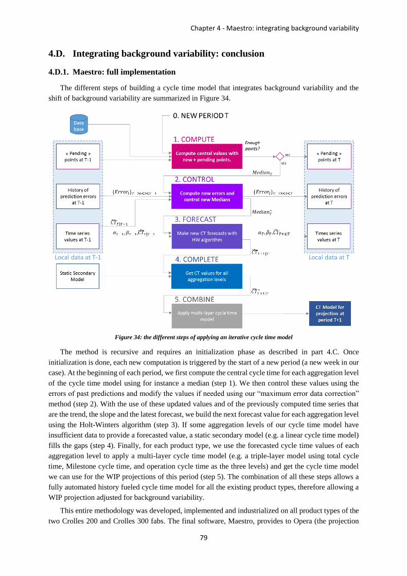
Chapter 4 - Maestro: integrating background variability
79
4.D. Integrating background variability: conclusion
4.D.1. Maestro: full implementation
The different steps of building a cycle time model that integrates background variability and the
shift of background variability are summarized in Figure 34.
Figure 34: the different steps of applying an iterative cycle time model
The method is recursive and requires an initialization phase as described in part 4.C. Once
initialization is done, each new computation is triggered by the start of a new period (a new week in our
case). At the beginning of each period, we first compute the central cycle time for each aggregation level
of the cycle time model using for instance a median (step 1). We then control these values using the
errors of past predictions and modify the values if needed using our “maximum error data correction”
method (step 2). With the use of these updated values and of the previously computed time series that
are the trend, the slope and the latest forecast, we build the next forecast value for each aggregation level
using the Holt-Winters algorithm (step 3). If some aggregation levels of our cycle time model have
insufficient data to provide a forecasted value, a static secondary model (e.g. a linear cycle time model)
fills the gaps (step 4). Finally, for each product type, we use the forecasted cycle time values of each
aggregation level to apply a multi-layer cycle time model (e.g. a triple-layer model using total cycle
time, Milestone cycle time, and operation cycle time as the three levels) and get the cycle time model
we can use for the WIP projections of this period (step 5). The combination of all these steps allows a
fully automated history fueled cycle time model for all the existing product types, therefore allowing a
WIP projection adjusted for background variability.
This entire methodology was developed, implemented and industrialized on all product types of the
two Crolles 200 and Crolles 300 fabs. The final software, Maestro, provides to Opera (the projection

Part Two - Integrating variability (in production management tools)
80
software) the cycle time models for all product types of both Crolles fabs. Overall, cycle time forecasts
using Holt-Winter algorithm are made weekly on more than 16000 aggregation levels (Milestones and
Operations for each product-type), building around 80 different cycle time models (some of which are
shown in Figure 29, page 72). Maestro refreshes the cycle time models weekly by running as a
programmed task on a network computer, and allows Opera to generate the WIP projection that defines
all the objectives of the fabs in terms of activities to achieve, resources to allocate, required Overall
Equipment Efficiencies… By better integrating the background consequences of variability, we
effectively improve the tractability of the manufacturing system and therefore help reduce one of the
consequences of variability.
4.D.2. Analyzing the results
A generally good idea when it comes to implementing new works or algorithms is to test for the
improvements provided. The improvements provided by our new tool was of course a priority for the
implementation of the solution. Yet, measuring the results provided by a new cycle time model is not
all that simple. One could think that since the Holt-Winter algorithm aims at predicting future cycle
times, a natural possibility would be to compare the difference (or Mean Squared Error) of the cycle
time values provided to the actual cycle time values. However, applying this measure would translate a
misunderstanding in the objective of a cycle time model… Indeed, as we mentioned in the beginning of
this chapter, the objective of a cycle time model is to provide a flow movement that allows a WIP
planification as close as possible to the natural behavior of the system, so as to minimize the number of
actions to take on the system to achieve the flow movement that was planned. Through this objective,
we understand that what we try to achieve with WIP projections and cycle time models is what is called
a “self-fulfilling prophecy”. In this context, we indeed want the future to be as close as possible as what
the cycle time model provided, but the difference between the two actually translates a mix of successful
actions on the system to respect the planification and of correct predictions.
Evaluating the quality of a cycle time model is therefore far more complicated that one could think
at first sight. For our industrial application, the evaluation was done through a close collaboration with
the engineers of the Industrial Engineering team responsible for the WIP projection. For several months,
WIP projections were made using both the old and the new cycle time models, and the ability of
production teams to achieve the objectives provided by the WIP projections based on both models was
compared. The official industrialization of Maestro was decided after consistent validation from the
Industrial Engineering team that the cycle time models from Maestro resulted in more coherent and
achievable targets.

Chapter 5 - The concurrent WIP: a solution to analyze complex systems
81
Chapter 5
5. The concurrent WIP: a solution to
analyze complex systems
Chapter 4 presented a solution to integrate the background consequences of workflow variability to
the projection tool of a manufacturing system. By increasing the quality of the projection/planification,
the work in chapter 4 allows taking more suitable actions on the manufacturing system to increase its
tractability.
As explained in chapter 1 and chapter 2, workflow variability materializes locally at the process-
cluster (toolset) level, as the result of the interaction between the incoming workflow and the process-
cluster. The ability of process-clusters to efficiently treat incoming workflow is therefore a major aspect
in workflow variability. However, as we explained in chapter 3, all the different sources of variability
add up and affect the performance of these process-clusters. In order to efficiently integrate the
consequences of variability, it is therefore important to integrate all of these effects in the various models
developed. This starts by measuring the actual performances of process-clusters, which standard
analytical tools such as the OEE [64] are unable to fully measure because of the complex interactions
between the numerous sources of variability. Chapter 5 aims at improving such measures.
We introduce in chapter 5 a new notion: the Concurrent WIP. This notion translates a shift from
looking at a process-cluster from the tools point-of-view to the products point-of-view, and effectively
allows us to measure the aggregated response of a process-cluster to incoming flow. By applying a
workload interpretation of Little’s law on each jobs’ time window, and studying the process-clusters’
aggregated response through several formulas and graphs, we show how the Concurrent WIP method is
able to precisely capture the capacity response of the system. We show through a case study from the
semiconductor industry that we can measure not only the average capacity of a process-cluster, but also
any capacity dependency to the workload as well as the variability of the clusters’ capacity. Finally, we
discuss further applications of our new approach to allow a better modelling and better tractability of
complex systems.
The work presented in this chapter was partly presented at the 2016 International Conference on
Modeling, Optimization & Simulation (MOSIM) [3] and further improved before being submitted to
the journal of IEEE Transactions on Automation, Science and Engineering (TASE).
Part Two - Integrating variability (in production management tools)
82
5.A. The problem with simple models applied to complex (variable)
systems
5.A.1. Simple bottom/up models
The fundamental purpose of production management tools is to take or allow taking actions on
physical systems in order to improve these ones. The tools however do not base their “reasoning” on the
physical systems but on virtual representations of these systems, which are called models. As the models
drive the tools, the effectiveness of the actions taken by the tools can only be as good as the accuracy of
the models that describe the physical systems.
Most models used in current production management tools are built to deal with regular systems that
can be described using various information about them in a bottom/up approach. Queueing theory for
instance can accurately model simple systems with just a handful of parameters about these systems.
Most queuing theory models however have a few underlying assumptions such as serial processes with
no overlapping (in layman’s term: “each process on a tool starts right after the end of the previous
process”), independence in the arrivals, identical tools, independent downtimes and process-times…
These assumptions help the simplicity of the models and in most cases, work pretty well.
When it comes to HMLV production, or more generally complex manufacturing systems, these
assumptions reach their limit of validity. Indeed, all the sources of variability that we listed in chapter 3
have a significant impact on the system, but are either poorly or not at all taken into account in most
bottom/up models. The reason however, is not simply outdated models, but has to do with the way these
models are built and what we can call a limit of information…
5.A.2. The limit of information
Regular models, those made to describe simple systems, are built with a bottom/up approach. This
means that they aim at describing the output of the system by adding up separate information about the
system and modelling how these inputs combine to produce the output. For instance, a standard practice
to study toolsets in semiconductor manufacturing, as shown by Martin [23], is to build a capacity model
from the theoretical capacity of all tools (e.g. 8 jobs per hour), to then individually measure all
inefficiencies such as downtimes, idle-times, setup-times… (e.g. 3 jobs per hour) and to remove these
inefficiencies to get an estimation of the overall capacity (e.g. 8-3=5 jobs per jour). This is a reasonable
approach used broadly that works perfectly for regular systems.
The problem however arises when we try to apply this approach to complex systems. A complex
system, if we take the definition literally, is a system where the amount of information to properly
describe it is extremely high. Potentially, all this information is important as a small change on the inputs
can have big impact on the outputs. As the simple bottom/up approaches are necessarily composed of
many assumptions in order to simplify the model, lots of important information can be lost when applied
to complex systems and have negative impacts on the quality of the model. For instance, imagine a
toolset of 4 tools treating lots in parallel. In a normal system, the lots and the tools would be almost
similar. In this case, only 2 parameters are required to calculate the throughput of the toolset under
regular assumptions: the average process-time of a tool (PT) and the number of tools M
(throughput=M/PT). If we simply add a bit of complexity by having 4 different product-types and
flexible qualifications, we now need to know at least the tools qualifications on each product-type and
the process-time of each product-type, i.e. we need at least an extra 4 × 4 = 20 parameters to calculate

Chapter 5 - The concurrent WIP: a solution to analyze complex systems
83
the throughput. Obviously, this is still an extreme over-simplification as all the sources of variability
that we listed in chapter 3 interact and affect the output: There are many different parameters that have
significant impact on the output of the system and the simplifying assumptions that are made to describe
simple systems with a bottom/up approach do not hold in the case of complex systems.
5.A.3. The existence of a measurable output
However, the same principle we applied to the background consequences of variability can be
applied in the analysis of local systems: even though the way all parameters interact with each other to
produce an output is too complicated to handle, the output may not be too complicated to understand.
For instance, we know gravity comes from insanely complicated quantum mechanics interactions: The
sources of fluctuations and the interactions between all these sources is so complex that no bottom/up
model is able (as of 2017) to describe how the quantum mechanics system that is our universe is able to
produce the macroscopic effects that form the planets and the galaxies. However, by measuring some
of the outputs of these effects (like the gravitational constant), we are able to develop simplified models
(Newton’s law of universal gravitation) that accurately describe the system on the scale we are interested
in. As variability is the quantum mechanics of complex manufacturing systems, we need our
gravitational constant to allow us deriving simplified models. In other words, in order to better analyze
complex systems subject to high levels of variability, we need tools to directly analyze the outputs of
the systems, and not rely on a bottom/up approach.
The first part of the solution is done naturally for almost all models: split the problem into smaller
problems, i.e. group process-units together. This is generally done by creating toolsets (treating identical
queues of products). We showed in section 2.E that toolsets could be inaccurate, and proposed to make
groups (process-clusters and highly connected process-clusters) based on the ability of process-units to
work together to treat an identical flow of products. With this first step in mind, we need a method to
better analyze these process-clusters…
5.B. A novel approach: the Concurrent WIP
5.B.1. Definition of the concurrent WIP
As we have set rigorously the bounds of our problem with the notion of process-clusters, we are left
with smaller, but still unsolved, problems: how can we accurately analyze the real system in a way that
allows encapsulating the combined effects of the different sources of variability? Classical measures of
cycle time, throughput, WIP levels… are starting points, but they fail at really measuring the system,
i.e. the behavior of the process-cluster, since they all directly depend on other parameters: cycle time
and WIP levels are affected by saturations, throughput is dependent on the arrival-rate…
Changing reference frame: the products point-of-view
The novel approach we propose, and that we call the Concurrent WIP (CWIP), actually starts by
changing the reference frame: instead of classically studying the system from the process-clusters point-
of-view in a bottom/up approach, we propose to study it from the jobs’ point-of-view, allowing local
measures of the output of the system as seen by each job. The CWIP is a notion defined for every job.
Hence, we place ourselves at an individual process-cluster and consider a given job p. The reference
frame of job p is the time interval between its arrival at the process-cluster and its actual process start;
which we call its Effective Waiting-Time (𝐸𝑊𝑇𝑝). For every other job i, we call 𝑊𝐿𝑖 its Workload
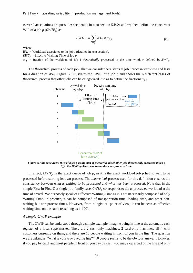
Part Two - Integrating variability (in production management tools)
84
(several acceptations are possible; see details in next section 5.B.2) and we then define the concurrent
WIP of a job p (𝐶𝑊𝐼𝑃𝑝) as:
𝐶𝑊𝐼𝑃𝑝 = ∑ 𝑊𝐿𝑖 × 𝑥𝑖,𝑝
∀𝑖
(8)
Where
𝑊𝐿𝑖 = WorkLoad associated to the job i (detailed in next section).
𝐸𝑊𝑇𝑝 = Effective Waiting-Time of job p.
𝑥𝑖,𝑝 = fraction of the workload of job i theoretically processed in the time window defined by 𝐸𝑊𝑇𝑝.
The theoretical process of each job i that we consider here starts at job i process-start-time and lasts
for a duration of 𝑊𝐿𝑖. Figure 35 illustrates the CWIP of a job p and shows the 6 different cases of
theoretical process that other jobs can be categorized into as to define the fractions 𝑥𝑖,𝑝.
Figure 35: the concurrent WIP of a job p as the sum of the workloads of other jobs theoretically processed in job p
Effective Waiting-Time window on the same process-cluster
In effect, 𝐶𝑊𝐼𝑃𝑝 is the exact queue of job p, as it is the exact workload job p had to wait to be
processed before starting its own process. The theoretical process used for this definition ensures the
consistency between what is waiting to be processed and what has been processed. Note that in the
simple First-In-First-Out single-job-family case, 𝐶𝑊𝐼𝑃𝑝 corresponds to the unprocessed workload at the
time of arrival. We purposely speak of Effective Waiting-Time as it is not necessarily composed of only
Waiting-Time. In practice, it can be composed of transportation time, loading time, and other non-
waiting but non-process-times. However, from a logistical point-of-view, it can be seen as effective
waiting-time on the same reasoning as in [20].
A simple CWIP example
The CWIP can be understood through a simple example: imagine being in-line at the automatic cash
register of a local supermarket. There are 2 cash-only machines, 2 card-only machines, all 4 with
customers currently on them, and there are 10 people waiting in front of you in the line. The question
we are asking is: “what is your true queuing line?” 10 people seems to be the obvious answer. However,
if you pay by card, and most people in front of you pay by cash, you may skip a part of the line and only
Chapter 5 - The concurrent WIP: a solution to analyze complex systems
85
effectively wait, for instance, behind 5 people. Moreover, you actually partly wait behind the 4
customers that were on the machines when you arrived. However, these 4 customers do not have the
same weight as the other ones as they have partly finished processing their workload… The CWIP,
computed a posteriori, will rigorously answer this question.
5.B.2. Workload measures
It is essential to define 𝐶𝑊𝐼𝑃𝑝 in terms of workload, and not in terms of number of jobs because
different job-families can have different expected process-time. The workload is therefore a measure of
the expected occupancy weight that a job has on the process-cluster. Furthermore, a workload view
allows to accurately take into account partial jobs as is shown in Figure 35.
As the process-units can be heterogeneous, different workload measures can be given, depending on
the underlying need. We define here 3 different workload measures, namely the Minimum Process-Time
(MPT), the Average Process-Time (APT), and the Optimal Process-Time (OPT). The MPT is the
sustainable theoretical Minimum Process-Time over all process-units qualified to process the given job-
family. The APT is the observed Average Process-Time for the given job-family at the process-cluster.
The OPT is the average Process-Time a process-cluster will achieve on the job-family when it achieves
Optimal performances; OPT is a theoretical time that can be computed using balancing algorithms or
linear models to achieve best overall capacity or cycle time using the same logic as Ignizio [21]. In
simple systems these workload units are equivalent, however in complex system they have important
differences. For instance, comparing APT with OPT provides a good measure of the loss of capacity
caused by execution problems as it allows comparing what actually happened to what could have
happened (whereas the MPT is not always achievable since different tools can have different process-
times).
In the previous supermarket example, the workload of the customers can be linked to the number of
items they have in their shopping kart. For each number of items in the shopping kart, you expect a
different process-time. For instance, customers with only 1 article may expect an average process-time
of 1 minute, when customers with 10 articles may expect an average process-time of 3 minutes. In order
to define your true queuing line, it makes more sense to speak in terms of workload and say “my queuing
line was 15 minutes of expected process-time” rather than “my queuing line was 10 customers”. Firstly
because the information is more precise, and secondly because all the variations in the time it took “15
minutes of expected process-time” to be actually processed will give us information about the process-
cluster (here the automatic cash register)…
5.B.3. Capacity estimations using the Concurrent WIP
The limit of models hypotheses
Measuring or estimating the capacity of a system is useful for many fields of application with
capacity planning being the main one. For simple systems, the capacity can be estimated by making
hypothesis on the system to apply a formula suited for the theoretical model. For instance, classic
hypotheses are: single job-family, identical process-units, sequenced processes with no overlapping and
no time between a process-end and the next process-start. With such hypotheses, the capacity of the
process-cluster is the sum of the service-rates namely 𝑀
𝑃𝑇 with M the number of process-units and PT the
mean process-time. For instance, having 10 process-units with 2 hours process-times, the process-cluster
capacity is 5 jobs/hour. When these hypotheses do not hold, one can empirically estimate the capacity
by the departure-rate of the process-cluster. However, departure-rates show two major limitations: first,
Part Two - Integrating variability (in production management tools)
86
they are irrelevant measures of capacity if the queue ever becomes empty during the measurement, hence
the need for carefully chosen time-windows; second, they are expressed as a number of jobs, which is
not meaningful for complex system with heterogeneous job-families.
In many real-life situations, estimating the capacity is done empirically by identifying and measuring
individual sources of inefficiencies and removing them to the theoretical capacity to get an estimation
of the actual capacity. However, as stated before, applying this method to complex process-clusters can
results in high inaccuracies since not all the information about the system is known.
Local interpretation of Little’s law
Little's Law, recently refined by himself [68], allows to measure the throughput of a system (TH) on
a given time-window by counting the average number of jobs in the system (WIP) and the average Cycle
Time (CT): TH = WIP/CT. For process-clusters, this throughput is equal to the arrival-rate if no jobs
are waiting at the end of the measuring period, and is equal to the capacity of the system during this
period if there was always at least one job waiting to be processed during this time-window. Therefore,
using Little’s Law to measure the capacity of a process cluster is in theory possible, giving that the time
windows chosen satisfies the aforementioned condition.
However, the unit of WIP (number of items) in Little’s Law makes two separate measures incoherent if
the mix of job-families changes (since the average process-time changes) and therefore seems
impractical to apply to complex systems. The concurrent WIP passes these two challenges, firstly
because by definition a CWIP is always associated to a job that was waiting; secondly because the unit
of CWIP being a workload, the measure is independent of the mix. Therefore, we can derive a CWIP
adaptation of Little’s Law as shown by Equation (9):
𝐶𝑝 =
𝐶𝑊𝐼𝑃𝑝
𝐸𝑊𝑇𝑝 (9)
Where:
𝐶𝑝 = The capacity seen by job p during its Effective Waiting-Time.
𝐶𝑊𝐼𝑃𝑝 = The concurrent WIP of job p.
𝐸𝑊𝑇𝑝 = The Effective Waiting-Time of job p.
Note that we directly wrote a capacity term in equation (9) and not a throughput, since a CWIP
always measures the throughput when this one is equal to the capacity of the process-cluster. For each
job, using the CWIP, we can therefore measure a snapshot of the capacity of the process-cluster as seen
by this job. Applied to the supermarket example, equation (9) tells us that by measuring your CWIP
(e.g. 15 minutes of expected process-time) and the time you waited in-line (e.g. 5 minutes), you can tell
which capacity the cash registry process-cluster had during your time window (e.g. 3 minutes of
expected-process-time per minute, which is the capacity of the entire cash registry).
Aggregating separate capacity measures
As equation (9) measures a capacity for each job (seen by each job), we can measure many capacity
realizations of the process-cluster (one by job), and use these realizations to aggregate useful measures
of capacity. We therefore propose the following formula to compute from historical data the average
weighted capacity of a process-cluster seen by all jobs i during a given period of time:
𝐶̅ =
∑ (𝐶𝑊𝐼𝑃𝑖 × 𝐶𝑖)𝑖
∑ 𝐶𝑊𝐼𝑃𝑖𝑖 (10)
Equation (10) gives the average capacity seen by all jobs weighted by their concurrent WIP. This
weight is important as it gives a proportionally higher importance to jobs that witnessed the systems’
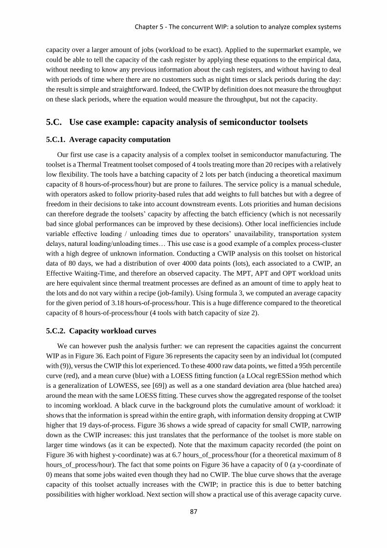
Chapter 5 - The concurrent WIP: a solution to analyze complex systems
87
capacity over a larger amount of jobs (workload to be exact). Applied to the supermarket example, we
could be able to tell the capacity of the cash register by applying these equations to the empirical data,
without needing to know any previous information about the cash registers, and without having to deal
with periods of time where there are no customers such as night times or slack periods during the day:
the result is simple and straightforward. Indeed, the CWIP by definition does not measure the throughput
on these slack periods, where the equation would measure the throughput, but not the capacity.
5.C. Use case example: capacity analysis of semiconductor toolsets
5.C.1. Average capacity computation
Our first use case is a capacity analysis of a complex toolset in semiconductor manufacturing. The
toolset is a Thermal Treatment toolset composed of 4 tools treating more than 20 recipes with a relatively
low flexibility. The tools have a batching capacity of 2 lots per batch (inducing a theoretical maximum
capacity of 8 hours-of-process/hour) but are prone to failures. The service policy is a manual schedule,
with operators asked to follow priority-based rules that add weights to full batches but with a degree of
freedom in their decisions to take into account downstream events. Lots priorities and human decisions
can therefore degrade the toolsets’ capacity by affecting the batch efficiency (which is not necessarily
bad since global performances can be improved by these decisions). Other local inefficiencies include
variable effective loading / unloading times due to operators’ unavailability, transportation system
delays, natural loading/unloading times… This use case is a good example of a complex process-cluster
with a high degree of unknown information. Conducting a CWIP analysis on this toolset on historical
data of 80 days, we had a distribution of over 4000 data points (lots), each associated to a CWIP, an
Effective Waiting-Time, and therefore an observed capacity. The MPT, APT and OPT workload units
are here equivalent since thermal treatment processes are defined as an amount of time to apply heat to
the lots and do not vary within a recipe (job-family). Using formula 3, we computed an average capacity
for the given period of 3.18 hours-of-process/hour. This is a huge difference compared to the theoretical
capacity of 8 hours-of-process/hour (4 tools with batch capacity of size 2).
5.C.2. Capacity workload curves
We can however push the analysis further: we can represent the capacities against the concurrent
WIP as in Figure 36. Each point of Figure 36 represents the capacity seen by an individual lot (computed
with (9)), versus the CWIP this lot experienced. To these 4000 raw data points, we fitted a 95th percentile
curve (red), and a mean curve (blue) with a LOESS fitting function (a LOcal regrESSion method which
is a generalization of LOWESS, see [69]) as well as a one standard deviation area (blue hatched area)
around the mean with the same LOESS fitting. These curves show the aggregated response of the toolset
to incoming workload. A black curve in the background plots the cumulative amount of workload: it
shows that the information is spread within the entire graph, with information density dropping at CWIP
higher that 19 days-of-process. Figure 36 shows a wide spread of capacity for small CWIP, narrowing
down as the CWIP increases: this just translates that the performance of the toolset is more stable on
larger time windows (as it can be expected). Note that the maximum capacity recorded (the point on
Figure 36 with highest y-coordinate) was at 6.7 hours_of_process/hour (for a theoretical maximum of 8
hours_of_process/hour). The fact that some points on Figure 36 have a capacity of 0 (a y-coordinate of
0) means that some jobs waited even though they had no CWIP. The blue curve shows that the average
capacity of this toolset actually increases with the CWIP; in practice this is due to better batching
possibilities with higher workload. Next section will show a practical use of this average capacity curve.

Part Two - Integrating variability (in production management tools)
88
Figure 36 : concurrent WIP against observed capacities
These curves show that there is no such thing as “the” capacity of the system; instead, a workload-
dependent capacity must be considered. However, if a single value must be provided, the average
capacity of 3.18 (as measured above with equation (10)) appears to be a good estimate. The 95th
percentile curve (𝐶95) shows the capacity limit, i.e. the maximum achievable capacity. This capacity
limit can also be workload dependent, even though it seems to be more stable in our example. The
capacity limit enables to derive a Minimum Absorption Time (MAT) by capacity equation (9): the
minimum time it took to treat a workload amount of WL was 𝑊𝐿 𝐶95⁄ (𝑊𝐿). Next section shows a
practical use of the MAT.
5.C.3. Application to infinite capacity projection
Average and capacity limit curves (which are depicted in Figure 36) can be useful in infinite capacity
projections analysis (well described by [70]). In infinite capacity projections, projections of WIP are
first made considering a given fixed cycle time per operation (with each operation associated to a
process-cluster), without considering capacity limits. Capacity analysis is then done independently after
the projection: by comparing (for each process-cluster on a given period) the projected workload with
the capacity of the process-cluster, it shows where major bottlenecks will occur (if the projected
workload is bigger that the capacity, it is an indication of a major bottleneck to occur). However,
estimating capacity in complex process-clusters is a real challenge as mentioned earlier and capacity
analysis often suffer from wrong estimates of the capacities, resulting in unanticipated bottlenecks and
firefighting activities.
CWIP capacity curves can offer a significant improvement to these industrial engineering activities.
Assume, for instance, that infinite capacity projection has forecasted a workload of 15 days_of_process
for the next 4 days on the toolset of Figure 36. Based on concurrent WIP, Figure 36 tells that, for such
a workload, the capacity limit is 4.3 days_of_process/day and the average capacity is 3.7
days_of_process/day. This means that the fastest this toolset has ever absorbed 15 days_of_process is
in 15/4.3= 3.5 days (the Minimum Absorption Time MAT) and that, on average, the process cluster
Chapter 5 - The concurrent WIP: a solution to analyze complex systems
89
takes 15/3.7= 4.1 days to absorb this amount of WIP. Therefore, in this case, since the projection period
is 4 days, a bottleneck is likely to occur since it takes on average more than 4 days (4.1 days) to absorb
that much WIP. Nevertheless, if some measures are taken to achieve a high performance at this toolset
during this period (delaying preventive maintenance for instance), the bottleneck can be avoided since
toolset can absorb this amount of WIP in less than 4 days (MAT of 3.5 days).
5.C.4. Application to clearing functions
The non-linear relationship between the capacities of the process-clusters and the workload is a
known effect in the literature. The derivation of Clearing Functions (CFs), which provide a relationship
between throughput and WIP levels, is a relatively recent field of study intending to use non-linear
capacity models based on WIP quantities in production planning models. The use of CFs has proven
significant improvements in production planning tools and is considered a key element for future
production systems. Albey, Bilge, and Uzsoy [71] include an overview of recent research on Clearing
Functions.
One challenge CFs face however is the ability to derive functions that accurately describe the reality
when applied to complex environments. Indeed, the first reason is that measuring the true capacity of a
system is a more than challenging task. Secondly, CFs functions are generally represented as throughput
vs WIP level (in terms of number of jobs to process). As we explained in part 5.B.2, the choice of the
correct workload is crucial to measure correctly the capacity of a process-cluster. Both the units of
throughput (number of jobs processed per time unit) and of WIP levels (number of jobs to process) may
fail to capture the true capacity of a process-cluster in a complex environment. Indeed, let us take the
example of two measures of throughput on the same process-cluster but on two different time windows.
Let us assume that the WIP levels are the same for both measures and that the process-cluster has the
exact same capacity on both time windows (e.g. 100% up-time, 100% batch-rate, no inefficiencies
whatsoever…). If the mix of job-families is not the same on both periods, the workload on both periods
will be different (even though the WIP levels are identical). When measuring the time it takes to absorb
the WIP level in both cases, we will therefore get different times (because we have different workload)
and we will therefore measure different throughputs (if we base our approach on WIP levels). However,
as we mentioned before, the process-cluster has an identical capacity and behavior on both time
windows… In turn this means that measuring throughput vs WIP levels has high risk of giving
inconsistent results even when the behavior of the process-cluster stays rigorously the same, and can
only be applied for estimates in the future for identical job-families mix, as a different product-mix
would make the Clearing Function unfit.
Another application of the Concurrent WIP could therefore be the derivation of Clearing Functions
adjusted to the units of the capacity workload graphs. The Concurrent WIP would allow measuring the
performance of the past, and the change of units in the Clearing Functions would allow applying these
performances to future projections with a higher precision. The LOESS mean curve of Figure 36
measuring the historical clearing function, the parameters of the mathematical clearing function could
be fitted to minimize the distance to this curve in order to represent the average behavior of a real
process-cluster.
5.C.5. Measure of variability
As we covered the different aspects of workflow variability in part I of this manuscript, we have
explained that workflow variability, from a practitioner’s point-of-view, is the tendency to create high
workloads unexpectedly. Moreover, we established that both the inflow of the products and the process-

Part Two - Integrating variability (in production management tools)
90
clusters are responsible for a part of this variability. A process-cluster will create more workflow
variability if it suffers more capacity losses in the presence of workload (thus creating unexpected
accumulations of workload). As a tool that allows analyzing both workload and capacity, the Concurrent
WIP can provide a measure of this tendency to suffer capacity loss in the presence of workload. The
presence of workload is essential, as capacity loss (i.e. process-units unavailability or degraded
performances) is only problematic if it disturbs the flow of jobs. Assuming independency between
arrivals and the process-units behaviors is a way to not consider this dimension, but we cannot assume
this for complex process-clusters since this represents a massive loss of possibly important information.
Moreover, from a practitioner’s point-of-view, dependent behaviors are the rule, not the exception (at
least in semiconductor manufacturing).
To measure the tendency of a process-cluster to suffer capacity loss in the presence of workload, we
can look at the weighted variability of the capacity of the process-cluster. A visual way of measuring
this variability is simply the area of one standard deviation around the mean as is shown on Figure 36.
More rigorously, equation (11) gives a practical measure for the impactful variability of the capacity of
a process-cluster seen by all jobs i:
𝑉𝑐 =
∑ 𝛿𝑖 × (𝐶̅ − 𝐶𝑖) × 𝐶𝑊𝐼𝑃𝑖𝑖
𝐶̅ × ∑ 𝛿𝑖 × 𝐶𝑊𝐼𝑃𝑖𝑖
(11)
Where
𝐶𝑊𝐼𝑃𝑖 is the concurrent WIP of job i
𝐶̅ is the average capacity seen by jobs as calculated in (3).
𝛿𝑖 = 0 if 𝐶̅ − 𝐶𝑖 < 0, 𝛿𝑖 = 1 otherwise.
Note that only capacities below the measured average 𝐶̅ are taken into account: this is intended for
a practical use of the data as, as mentioned before, only capacity losses impact negatively the process-
cluster. Therefore, we do not want variability reduction to happen by cutting very good performances,
but only by reducing the bad ones. Moreover, the observed capacities are weighted by their associated
CWIP: indeed, a job observing a capacity loss impacting a high workload is proportionally more
important than a job observing a capacity loss impacting a small workload, as the capacity to generate
a queue is directly linked to the workload affected. With equation (11), we therefore compute the
average weighted deviation of capacity to the mean, restricted to capacities lower than the mean.
Including 𝐶̅ (the average capacity from equation (10)) in the denominator standardizes this deviation
relative to the mean.
Applied to the data of Figure 36, we calculated 𝑉𝑐=0.22, which means that on (weighted) average,
the capacity below the mean is distant by 22% from the mean. From our formula, we infer that two
distinct effects participate in the variability: first, local capacity losses affecting high workload
participate the most to variability (points with high x and low y values on our capacity graph Figure 36).
Second, the fact that the average capacity varies over workload (that the blue curve is not a horizontal
line) participates to the variability as it means more points are necessarily further away from the mean.
This impact can be well understood with a thought experiment: Let us imagine the initially empty
process-cluster represented by Figure 36 and start the inflow of jobs; let us assume an arrival rate of 3.5
hours_of_process/hour. As the queuing workload is initially empty, the capacity of the system is initially
smaller than the arrival rate (at around 2.5). The queuing workload will therefore start increasing. This,
in turn, will increase the capacity of the process-cluster up to the point where its capacity equals the
arrival rate. This workload will be a stable point: the system will tend to bring the workload to this
amount. We can therefore assume, by the mere interpretation of these capacity curves, that the particular

Chapter 5 - The concurrent WIP: a solution to analyze complex systems
91
system of Figure 36 will create high amount of queuing times by the simple fact that its capacity depends
on the workload. This tendency is however captured by the capacity variability factor of equation (11).
5.D. Perspectives for the use of Concurrent WIP
5.D.1. Queuing time estimates based on concurrent WIP capacity curves
An interesting perspective for the use of the concurrent WIP can be the development of queuing
theory formulas based on the capacity curves and measurements provided by the concurrent WIP.
Indeed, we can provide measures for the capacity, the dependency to workload, and the variability of
the overall capacity. Provided that measures of the variability of the inflow can be computed, we believe
that the concurrent WIP could open the door to a brand new way of deriving queuing time estimates for
complex process-clusters and reduce the gap between theoretical and real complex systems.
The first step for this approach would be to make aggregate measures of the variability of the inflow
of jobs. The current measure queuing theory provides (the coefficient of variation of inter-arrival times)
is not suitable for complex process-clusters as it does not take into account the multi job-family
parameter nor the dependency in the arrivals. We believe that an aggregate measure of the variability of
the inflow should consider workload with the same units considered in the concurrent WIP approach.
The second step should validate the potential of the concurrent WIP metrics to quantify the overall
performances of the process-cluster. One could do so by quantifying how simple known effects change
concurrent WIP parameters (for instance increasing the number of parallel process-units in simple
systems should decrease the capacity variability factor).
Moreover, dependent behaviors being common in complex environment, it would be essential to
derive methods to estimate the impact of the dependency between the arriving flow and the process-
cluster to adjust the impact of the variability of both the inflow and the capacity of the process-cluster.
5.D.2. Situational comparison
As the concurrent WIP allows to capture efficiently the aggregated response of any process-cluster
to incoming flows, we believe it can be a powerful tool for situational comparison. For instance, one
can compare a simulation model with the real system the simulation tries to model. Indeed, developing
a simulation model for a complex process-cluster requires big investments in terms of development, data
gathering and treatment, and simplifying assumptions are often made to reduce development cost. By
running a concurrent WIP analysis both on historical data and on the results of the simulation model fed
with the same inflow of jobs, and comparing both capacity curves, one could quickly tell the differences
between the real process-cluster and its simulation twin, along with useful information on where the
difference stands.
One could also use the concurrent WIP to compare the performances of the same process-cluster
over time by running a concurrent WIP analysis on the same process-cluster but on different time
windows. This can be especially useful for production managers who set goals to their production teams.
For instance, one can follow the performances of a process-cluster over time to track any performance
issues. One might want to follow the performances over time to improve a given process-cluster, for
instance focusing on variability reduction using the capacity variability factor 𝑉𝑐 that we provided in
equation (11).
Part Two - Integrating variability (in production management tools)
92
5.D.3. Concluding on the Concurrent WIP and the integration of variability
As discussed earlier, high levels of variability in complex systems mean that many parameters and
many sources of variability interact with each other in a way that is too complex to properly model.
However, we are able in simple models to explain how the main components act: an extra tool will add
capacity, more downtimes and more downtime variability will increase cycle time, higher product-mix
in the presence of batches and setups will increase the average WIP levels and therefore cycle times.
In order to combine these main components in models that can accurately describe the complex
reality, we need to fit these models based on precise measures from the real systems, in the same way
physicists fitted Newton’s law of gravitation by measuring the gravitational constant. The Concurrent
WIP offers such perspectives, as the analysis of the Concurrent WIP data such as the capacity-workload
graphs (and curves) and the CWIP equations measuring average capacity and variability give detailed
information about the system studied while removing the noise from product-mix that classic
throughput-WIP analysis were suffering from.
It is essential that approaches such as the Concurrent WIP get developed further as a gap currently
exists between theoretical models and real complex systems, with little to no way of communication
between them. These approaches should allow future models to incorporate different variability
components factor to their parameters. The objective of such models being to decrease this factor over
time as more and more sources of variability get quantified and added as parameters into the models.
Chapter 6 - Dependency effects: improving the knowledge on the sources of variability
93
Chapter 6
6. Dependency effects: improving the
knowledge on the sources of variability
Chapter 5 showed the importance of accurately measuring the true performances of process-clusters
(toolsets) in order to further integrate workflow variability into the different tools. Indeed, as the
different models in use in a manufacturing environment are intended to predict the behaviors and
response of the different process-clusters, it is essential to start off with the correct information.
However, if we want the models to correctly integrate the important aspects of workflow variability (and
its impact on cycle time and tractability), we need to have a proper understanding of how the different
sources of variability create this workflow variability.
One mechanism which we believe creates workflow variability is what we call “dependency
effects”. Contrary to the common assumption that independent and identically distributed variables can
accurately describe the phenomenon involved in workflow variability, we believe that the sequences of
events play a major role in workflow variability. We therefore investigate in this chapter the effects of
dependencies on three major elements of workflow variability: downtimes, process-times and arrivals.
We propose a method to do so by running simulations using actual shop floor data, and show through
our results that dependencies can actually be responsible for a far bigger amount of workflow variability
than previously suspected, and that developing tools in this direction could greatly improve the
integration and reduction of workflow variability. We also build a reasoning from these results which
suggests that a key ingredient in workflow variability is the correlation between arrivals at the different
process-clusters and the behavior of these process-clusters.
The work and results in chapter 6 were partly presented at the 2017 International Conference on
Industrial Engineering and Systems Management (IESM). Complementary work was conducted after
this submission and extra results which were not included in the IESM paper were included in this
chapter as to give a full picture on the complex behaviors of real-world process-clusters.

Part Two - Integrating variability (in production management tools)
94
6.A. The need to understand the mechanisms of variability
6.A.1. A technological maturity to model complex effects
From the previous chapters of this manuscript, we can understand that workflow variability
(especially in complex manufacturing systems) presents itself as an extremely complex information that
is not yet understood and well taken into account. For instance, workflow variability is so complex that
it has different consequences on different scales that cannot be accounted for in a bottom/up approach
(as we discussed in chapter 4). Workflow variability can be so complex that simple characteristics such
as the capacity of a system cannot be accurately derived using classic methods because of the crushing
amount of parameters and information that come to play to build them (which led us to derive a new
tool, the concurrent WIP, in chapter 5).
Workflow variability can be extremely complex, however we try to model it with very simple tools
and models. Early models, developed in the first half of the 19th century, had to be derived
mathematically as there was basically no other way to approach the problem. As so, it was reasonable
to approach the problem by making assumptions on how the systems worked, how the different sources
of variability behaved, and how the different parts interacted with each other. Such approaches led to
brilliant queuing equations such as those presented in Factory Physics, which do a great job modelling
simple systems, but have a clear limit when it comes to variability in complex systems. One century
later, we now have both the technology and the data to investigate how complex systems behave, we do
not need to rely on assumptions anymore, but can conduct simulation experiments and work on real
data.
In order to integrate variability further, we therefore need to get a deeper knowledge of the root
mechanisms that make sources of variability act on the system and generate higher cycle times and
higher uncertainties in the real world. The idea behind being that, even though the real interactions might
be too complicated to grasp, some general rules on which we can build future simple models might just
lie in the data: some complicated behaviors that have an impact on cycle time can be understood,
quantified, and fitted into future models.
6.A.2. Suspicions of dependency effects
Sources of variability have been intensely investigated in both the literature and the industry, and
tool downtimes, arrivals variability as well as process-time variability are recognized as major sources
of variability in the sense that they create higher cycle times (see chapter 3 for a review and discussion).
As a consequence, these factors are widely integrated into queuing formulas and simulation models with
the objective to better model the complex reality of manufacturing facilities. One commonly accepted
assumption in the development of these models is that the variables that describe these events (MTBF,
MTTR, process-times, time between arrivals, etc.) are independent and identically distributed (i.i.d.)
random variables. However, many authors ([10], [26], [34], [54], [71]) have discussed this point in the
limitations of classical models, and a few elements from industrial data also question the viability of this
assumption. For instance, we have shown in section 3.B.2 an example of dependent process-times which
might increase the overall workflow variability. Another example is shown in Figure 37: Figure 37.A
shows the number of arrivals per week at a toolset from STMicroelectronics Crolles300 fab, while
Figure 37.B shows arrivals per week generated using the same inter-arrival distribution as in Figure
37.A, but assuming independence of arrivals.
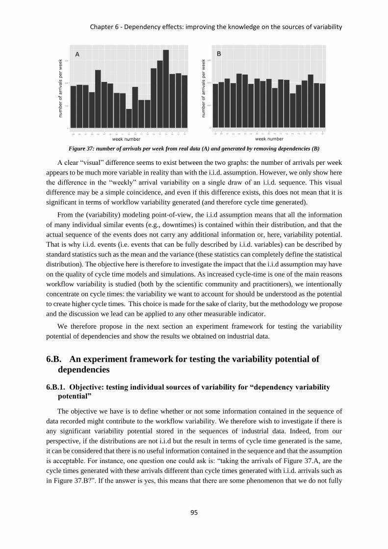
Chapter 6 - Dependency effects: improving the knowledge on the sources of variability
95
Figure 37: number of arrivals per week from real data (A) and generated by removing dependencies (B)
A clear “visual” difference seems to exist between the two graphs: the number of arrivals per week
appears to be much more variable in reality than with the i.i.d. assumption. However, we only show here
the difference in the “weekly” arrival variability on a single draw of an i.i.d. sequence. This visual
difference may be a simple coincidence, and even if this difference exists, this does not mean that it is
significant in terms of workflow variability generated (and therefore cycle time generated).
From the (variability) modeling point-of-view, the i.i.d assumption means that all the information
of many individual similar events (e.g., downtimes) is contained within their distribution, and that the
actual sequence of the events does not carry any additional information or, here, variability potential.
That is why i.i.d. events (i.e. events that can be fully described by i.i.d. variables) can be described by
standard statistics such as the mean and the variance (these statistics can completely define the statistical
distribution). The objective here is therefore to investigate the impact that the i.i.d assumption may have
on the quality of cycle time models and simulations. As increased cycle-time is one of the main reasons
workflow variability is studied (both by the scientific community and practitioners), we intentionally
concentrate on cycle times: the variability we want to account for should be understood as the potential
to create higher cycle times. This choice is made for the sake of clarity, but the methodology we propose
and the discussion we lead can be applied to any other measurable indicator.
We therefore propose in the next section an experiment framework for testing the variability
potential of dependencies and show the results we obtained on industrial data.
6.B. An experiment framework for testing the variability potential of
dependencies
6.B.1. Objective: testing individual sources of variability for “dependency variability
potential”
The objective we have is to define whether or not some information contained in the sequence of
data recorded might contribute to the workflow variability. We therefore wish to investigate if there is
any significant variability potential stored in the sequences of industrial data. Indeed, from our
perspective, if the distributions are not i.i.d but the result in terms of cycle time generated is the same,
it can be considered that there is no useful information contained in the sequence and that the assumption
is acceptable. For instance, one question one could ask is: “taking the arrivals of Figure 37.A, are the
cycle times generated with these arrivals different than cycle times generated with i.i.d. arrivals such as
in Figure 37.B?”. If the answer is yes, this means that there are some phenomenon that we do not fully
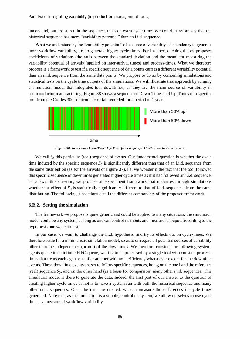
Part Two - Integrating variability (in production management tools)
96
understand, but are stored in the sequence, that add extra cycle time. We could therefore say that the
historical sequence has more “variability potential” than an i.i.d. sequence.
What we understand by the “variability potential” of a source of variability is its tendency to generate
more workflow variability, i.e. to generate higher cycle times. For instance, queuing theory proposes
coefficients of variations (the ratio between the standard deviation and the mean) for measuring the
variability potential of arrivals (applied on inter-arrival times) and process-times. What we therefore
propose is a framework to test if a specific sequence of data points carries a different variability potential
than an i.i.d. sequence from the same data points. We propose to do so by combining simulations and
statistical tests on the cycle time outputs of the simulations. We will illustrate this approach by running
a simulation model that integrates tool downtimes, as they are the main source of variability in
semiconductor manufacturing. Figure 38 shows a sequence of Down-Times and Up-Times of a specific
tool from the Crolles 300 semiconductor fab recorded for a period of 1 year.
Figure 38: historical Down-Time/ Up-Time from a specific Crolles 300 tool over a year
We call 𝑆0 this particular (real) sequence of events. Our fundamental question is whether the cycle
time induced by the specific sequence 𝑆0 is significantly different than that of an i.i.d. sequence from
the same distribution (as for the arrivals of Figure 37), i.e. we wonder if the fact that the tool followed
this specific sequence of downtimes generated higher cycle times as if it had followed an i.i.d. sequence.
To answer this question, we propose an experiment framework that measures through simulations
whether the effect of 𝑆0 is statistically significantly different to that of i.i.d. sequences from the same
distribution. The following subsections detail the different components of the proposed framework.
6.B.2. Setting the simulation
The framework we propose is quite generic and could be applied to many situations: the simulation
model could be any system, as long as one can control its inputs and measure its ouputs according to the
hypothesis one wants to test.
In our case, we want to challenge the i.i.d. hypothesis, and try its effects out on cycle-times. We
therefore settle for a minimalistic simulation model, so as to disregard all potential sources of variability
other than the independence (or not) of the downtimes. We therefore consider the following system:
agents queue in an infinite FIFO queue, waiting to be processed by a single tool with constant process-
times that treats each agent one after another with no inefficiency whatsoever except for the downtime
events. These downtime events are set to follow specific sequences, being on the one hand the reference
(real) sequence 𝑆0, and on the other hand (as a basis for comparison) many other i.i.d. sequences. This
simulation model is there to generate the data. Indeed, the first part of our answer to the question of
creating higher cycle times or not is to have a system run with both the historical sequence and many
other i.i.d. sequences. Once the data are created, we can measure the differences in cycle times
generated. Note that, as the simulation is a simple, controlled system, we allow ourselves to use cycle
time as a measure of workflow variability.

Chapter 6 - Dependency effects: improving the knowledge on the sources of variability
97
6.B.3. Measuring the effect of 𝑺𝟎
In our case, the effect of a sequence of downtimes is measured as the average cycle-time of the
agents in a simulation. In theory, this should be evaluated on an infinite horizon, that is until the measure
is stable enough, but it is in practice impossible since 𝑆0 is finite (as it represents real, empirical data).
As an alternative, to prevent any bias from a particular arrival sequence, we simply evaluate the long
term average cycle-time by running many simulations on different scenarios, that is on different arrival
sequences (following i.i.d. exponentially-distributed inter-arrival times). Let 𝐶𝑇𝑖,𝑗 be the mean cycle
time of agents from the simulation run on sequence i of downtimes and scenario j of arrivals; the effect
of 𝑆0 is then 𝐶𝑇̅̅̅̅0, the mean of mean cycle times from simulations that used 𝑆0 as an input.
6.B.4. Measuring the effect of i.i.d. sequences
To measure the effect of i.i.d. sequences, we generate many such sequences from the same
distribution; those sequences of downtimes (𝑆𝑖,𝑖≠0) are generated as random uniform permutations of 𝑆0.
Using the same procedure as for 𝑆0, we compute for each sequence 𝑆𝑖,𝑖≠0 its effect: 𝐶𝑇̅̅ ̅̅𝑖,𝑖≠0. Note that
we use the exact same scenarios of arrivals as for 𝑆0, this extra requirement insuring that any significant
difference between the population 𝐶𝑇̅̅̅̅𝑖,𝑖≠0 and the value 𝐶𝑇̅̅̅̅
0 comes strictly from the difference
between 𝑆𝑖,𝑖≠0 and 𝑆0.
The effect of a particular i.i.d. sequence is of virtually no interest as we want to measure the effect
of any i.i.d. sequence. This could be measured as the mean value of the 𝐶𝑇̅̅̅̅𝑖,𝑖≠0. However, measuring a
difference between 𝐶𝑇̅̅̅̅0 and 𝐶𝑇̅̅̅̅
𝑖,𝑖≠0 (between simulations using 𝑆0 or i.i.d. sequences) is not enough.
Indeed, statistical fluctuations are always to be expected. What we need to know is: is the difference
really more different than usual? To answer this question rigorously, we prefer measuring the effect of
i.i.d. sequences as a 95% confidence interval 𝐼95. We compute 𝐼95 as 𝜇 ∓ 2𝜎 where 𝜇 and 𝜎 are
respectively the mean and the standard deviation of 𝐶𝑇̅̅̅̅𝑖,𝑖≠0. Doing such calculation, we assume that
the 𝐶𝑇̅̅̅̅𝑖,𝑖≠0 points follow a Gaussian distribution: this is justified by the central limit theorem as each
point of our sample population is a mean, and by the fact that the underlying population 𝐶𝑇𝑖≠0,𝑗 most
likely follows a Gaussian distribution since the cycle time of each simulation comes from the
accumulation of many independent random effects. Moreover, this assumption is then verified on the
actual data generated.
As for the computation of 𝐶𝑇̅̅ ̅̅0, the right number of sequences and of scenarios must be carefully
chosen so as to get good estimates within reasonable running times. This is discussed in subsection
6.B.8.
6.B.5. Comparing the effects
Once 𝐶𝑇̅̅̅̅0 and 𝐼95 have been computed accurately, they must/can be compared using a standard
procedure for a statistical test: if 𝐶𝑇̅̅̅̅0 falls within 𝐼95, then it cannot be said that 𝑆0 has an effect
significantly different than that of an i.i.d. sequence; in the alternative, it can be assumed that 𝑆0 has a
different effect on cycle-time than an i.i.d. sequence. Figure 39 illustrates the three possible outcomes
of the test.

Part Two - Integrating variability (in production management tools)
98
Figure 39 : three possible outcomes when comparing 𝑪𝑻̅̅ ̅̅𝟎 to the sample population 𝑪𝑻̅̅ ̅̅
𝒊,𝒊≠𝟎
If 𝐶𝑇̅̅̅̅0 is on the left side of 𝐼95 (Figure 39.A), 𝑆0 carries a negative variability potential; If 𝐶𝑇̅̅̅̅
0 is
within 𝐼95 (Figure 39.B), it cannot be said that 𝑆0 carries any significant potential; if 𝐶𝑇̅̅̅̅0 is on the right
side of 𝐼95 (Figure 39.C), 𝑆0 carries a positive variability potential. Setting a 95% confidence interval
(or a p-value of 0.05) actually means, from a skeptic point-of-view, that there is a 5% chance for any
sequence tested that the results will turn out to be positive by pure randomness. It is therefore essential
to test different 𝑆0 sequences, and to compare the number of positives with the probability of getting
such results by “luck”. For instance, if we test 20 sequences, there is a 33% chance of having at least 2
false-positives out of the 20.
6.B.6. Handling uncertainties on 𝑪𝑻̅̅ ̅̅𝟎 and 𝑰𝟗𝟓
As 𝐶𝑇̅̅̅̅0 and 𝐼95 come from a finite population we created through simulation, the values we measure
are actually estimates of the true values (that we would get if we had an infinite population) and therefore
carry uncertainty (this means that if we repeat the same measures on different generated points, we
would get slightly different numbers). The actual value of 𝐶𝑇̅̅̅̅0 is contained in a confidence interval
around 𝐶𝑇̅̅̅̅0, which we call [𝐶𝑇̅̅̅̅
0]. The same applies to 𝐼95 : as we had to estimate 𝐼95, we are not certain
of the two limits of this interval, however 𝐼95 is most likely contained within inner/outer limits which
we call 𝐼95− and 𝐼95
+ . Figure 40 illustrates this point.
Figure 40 : uncertainty areas around 𝑪𝑻̅̅ ̅̅𝟎 and 𝑰𝟗𝟓
Chapter 6 - Dependency effects: improving the knowledge on the sources of variability
99
We can see on Figure 40 the interval [𝐶𝑇̅̅̅̅0] as well as two grey areas ( 𝐼95
+ − 𝐼95− ). If 𝐶𝑇̅̅̅̅
0 is far away
enough from 𝐼95 as for [𝐶𝑇̅̅̅̅0] and ( 𝐼95
+ − 𝐼95− ) not to touch, there is no problem as whatever value 𝐶𝑇̅̅̅̅
0
takes within [𝐶𝑇̅̅̅̅0], and whatever value 𝐼95 takes within ( 𝐼95
+ − 𝐼95− ), the answer to a significant
difference or not stays the same (In layman’s terms, 𝐶𝑇̅̅̅̅0 and 𝐼95 can wobble as much as they want in
their respective intervals, being in one of the cases of Figure 40 will mean staying in this case). The
problem arises when the uncertainty areas of [𝐶𝑇̅̅̅̅0] and 𝐼95 overlap: depending on what true value 𝐶𝑇̅̅̅̅
0
and 𝐼95 take inside their intervals, the answer can be different, and we can therefore not be sure of the
answer.
In order to get definitive answers, these uncertainty areas around 𝐶𝑇̅̅̅̅0 and 𝐼95 need to be reduced to
a point where they do not overlap anymore: if such case happens, we need to increase the number of
simulation runs as to decrease either [𝐶𝑇̅̅̅̅0] or the gap between 𝐼95
+ and 𝐼95− . Section 6.B.8 gives more
details on the computation of these values and the way to minimize the number of simulations in order
to get out of an overlap situation. There however needs to be a minimum amount of simulations in order
to start computing the uncertainty intervals. To test one 𝑆0 sequence, we decided to run simulations on
at least 20 i.i.d. sequences and 20 arrivals scenarios. Therefore, one simulation set is composed of at
least 400 simulations, and more if required by the uncertainty overlaps (up to a maximum that we
arbitrarily set to 10000 simulations).
As a complementary measure, we check, for each arrival scenario j, whether the mean of the
population 𝐶𝑇̅̅ ̅̅𝑖≠0,𝑗 is statistically different than 𝐶𝑇̅̅̅̅
0,𝑗. For each scenario j, we can answer this question
using a t-test and then count the number of times a scenario j gave 𝐶𝑇̅̅ ̅̅0,𝑗 respectively statistically smaller,
non-statistically different and statistically higher than the mean of the population 𝐶𝑇̅̅ ̅̅𝑖≠0,𝑗. As the
population 𝐶𝑇̅̅ ̅̅𝑖≠0,𝑗 represents average cycle times from identical simulation sets and parameters, only
with randomness coming from different draws of the parameters, we can assume that they follow a
normal distribution and can apply the t-test. These numbers are referred to as the “t-test triplets” in the
results section 6.C and are computed as a secondary test, keeping the previously explained methodology
as the main measure.
6.B.7. Ending simulations
Each simulation needs to be run over the period of time defined by the sequence 𝑆0 that is tested.
However, at the end of this period of time, some agents may have accumulated in the simulation. Cutting
the simulation abruptly can either lead to the loss of the cycle time of these agents or an underestimation
of their cycle time depending on how the information is recorded in the simulation.
In order to prevent from such effects, we decided to stop the arrivals after the time duration defined
by 𝑆0, and continue the simulation until all lots have exited the simulation. We also chose to leave the
tool up after the end of the given up/down sequence. This was first motivated by the fact that any other
decision could introduce biases to the results; secondly, by having a similar end to all simulations, we
actually slightly underestimated the difference between the historical sequence and its i.i.d. counterparts:
this only strengthens any significant difference.
6.B.8. Optimizing the number of simulation runs
As we previously mentioned, the uncertainties on 𝐶𝑇̅̅̅̅0 and 𝐼95 might be too high to properly answer
the question of statistically significant difference, and in turn, force to run more simulations until the
uncertainties are low enough. One way to be sure that these uncertainties are not biasing the results
Part Two - Integrating variability (in production management tools)
100
would be to run an extremely high amount of simulations, for instance generating 100 down sequences
and 100 arrival scenarios. The previous example would however require to run 10000 simulations. With
simulations that last a few seconds, running 10000 simulations can take more than an entire day. Testing
many different sequences could therefore take months. It is therefore essential to optimize the simulation
runs as to minimize the number of computation runs required to have no overlaps between the
uncertainty areas.
The first step is therefore to define rigorously [𝐶𝑇̅̅̅̅0], 𝐼95
+ and 𝐼95− in order to compute them after
each set of simulation following a new draw of an i.i.d. sequence of a new arrival scenario, thus allowing
to stop running simulations as soon as the uncertainty areas stop overlapping.
As the uncertainties on 𝐶𝑇̅̅̅̅0 and 𝐼95 come from the estimators, both uncertainty areas can be
computed straightforwardly: the standard deviation of the estimator for both the mean 𝜇 and the standard
deviation 𝜎 being respectively 𝜎
√𝑛 and
σ
√2(𝑛−1) where 𝜎 is the value of the estimator of the standard
deviation [72] and n is the sample size, we can define [𝐶𝑇̅̅̅̅0] as 𝐶𝑇̅̅̅̅
0 ∓2𝜎0
√𝑚, 𝐼95
− as μ ∓
(2σ −σ
√𝑛−
2σ
√2(𝑛−1)) and 𝐼95
+ as μ ∓ (2σ +σ
√𝑛+
2σ
√2(𝑛−1)) where 𝜎0 and σ are respectively the standard
deviation of 𝐶𝑇̅̅̅̅0,𝑗 and 𝐶𝑇̅̅̅̅
𝑖,𝑖≠0; n and m are respectively the number of different i.i.d. sequences and of
arrival scenarios; and μ is the mean of all 𝐶𝑇̅̅̅̅𝑖,𝑖≠0. To derive the formulas on 𝐼95
− and 𝐼95+ , we start with
the estimation of 𝐼95 (μ ∓ 2σ), and we subtract (𝐼95
− ) or add (𝐼95+ ) a standard-error for μ (
𝜎
√𝑛) and two
standard-errors for σ (σ
√2(𝑛−1)).
Comparing the areas after each set of simulation is however not sufficient: indeed, after the initial
400 simulations, the condition to either increase the number of sequences 𝑆𝑖 or the number of arrivals
scenarios is the same: an overlap between the red area and either of the grey areas of Figure 40. In order
to minimize the number of simulations, one option is to aim at the the biggest reduction in uncertainty
area per new simulation. Drawing another arrival sequence will reduce [𝐶𝑇̅̅̅̅0] whereas drawing
another 𝑆𝑖 sequence will reduce the gap between 𝐼95− and 𝐼95
+ . We therefore need to compute the decrease
in the uncertainty area per simulation for either case of making a new draw of arrivals or of downtime,
knowing that any new draw of arrivals needs to be run on all existing 𝑆𝑖 sequences and vice-versa. With
𝜎0 and σ being respectively the standard deviation of 𝐶𝑇̅̅̅̅0,𝑗 and 𝐶𝑇̅̅̅̅
𝑖,𝑖≠0; n and m being respectively the
number of different i.i.d. sequences and of arrival scenarios, by drawing a new arrival and running it on
all existing 𝑆𝑖 sequences, the gap reduction per simulation is:
4𝜎0 (1
√𝑚−
1
√𝑚 + 1)
𝑛
By drawing a new 𝑆𝑖 sequence and running this new sequence on all existing arrivals, the gap
reduction per simulation is:
2𝜎 (1
√𝑛+
2
√2(𝑛 + 1)−
1
√𝑛 + 1−
2
√2𝑛)
𝑚
To get these numbers, we simply take the size [𝐶𝑇̅̅̅̅0] with m arrival scenarios, and subtract to it the
size of [𝐶𝑇̅̅̅̅0] with m+1 simulations, which we divide by the n i.i.d. sequence we need to run the
simulation on (and do the same for the arrivals). Therefore, in order to know which set of simulations
to run after any set of simulations, one must compare these two values and run simulations on a new

Chapter 6 - Dependency effects: improving the knowledge on the sources of variability
101
arrival sequence if the first number is bigger, or run simulations on a new i.i.d permutation of 𝑆0 if the
opposite is true.
6.C. Testing downtimes, arrivals, and process-times for variability induced
by dependencies on industrial data
6.C.1. The three main sources of variability
From the literature review we presented in part 3, we pointed out that downtime events, arrivals
“variability”, and process-time “variability” are three of the most commonly discussed and pointed out
elements in the literature. It is also these three that are quantified as “variability factors” in widely spread
queuing equations such as found in Factory Physics. We therefore first focused our efforts on these three
factors to follow a “Pareto mindset”: as we are trying to dissect variability in order to explain it, we
might as well start with what generates the most variability. As discussed earlier in this manuscript,
arrivals “variability” is not really a source of variability, but is the result of many interactions between
sources of variability, and basically acts as a “super source of variability” at the process-cluster level.
6.C.2. Downtimes of C300 tools
Using the method described in section 6.B, we tested 19 tools from the C300 fab. For each of the
tools, we extracted the empirical sequence of Up-Times/Down-Times over a year. As the method
explains in section 6.B, for each empirical sequence, we drew many i.i.d. “sister” sequences and
combined these sequences in a simulation set with many different scenarios of arrivals. Each scenario
of arrivals being run with each of the Up-Time/Down-Time sequence. One implicit parameter for all
simulations of a single experiment was that the utilization rate of the tool was the same across all
simulations (as the utilization rate influences the cycle time). This also implies that the utilization rate
needs to be fixed beforehand. As utilization rate increases cycle time, there is more chance the difference
between 𝑆0 and its i.i.d. counterparts will be visible at higher utilization rates. Therefore, we decided to
evaluate the significance of the result at a utilization rate of 80% as it is a high utilization rate but is still
a realistic one.
Table 3 summarizes the results of our experiments. The results are normalized so that the average
cycle time for the sample i.i.d. sequences (𝜇) is equal to 100. Therefore, the values of 𝐶𝑇̅̅̅̅0 can be
compared straightforwardly between them and relative to the central cycle time for i.i.d. sequences 𝜇.
We also provide the confidence interval [𝐶𝑇̅̅̅̅0] and the 𝐼95
∗ value, which correspond to 𝐼95+ if 𝐶𝑇̅̅̅̅
0 is outside
𝐼95+ , 𝐼95
− if 𝐶𝑇̅̅̅̅0 is inside 𝐼95
− , or the corresponding conflicting confidence interval if there is an overlap of
the confidence intervals. The column “s” shows the result of our test: YES if there is a significant
different, NO if there is no significant different, and NA if we were not able to get a definitive answer.
We also add the “t-triplets” described in section 6.B.6. Tools with same letters are from the same tool
type.

Part Two - Integrating variability (in production management tools)
102
Table 3 : results of the experiment framework tested on 19 tools down/up sequences from STMicroelectronics
As Table 3 shows, out of the 19 historical sequences we tested, 3 did not show any significant
difference in the variability potential they carried compared to their i.i.d. counterparts, 13 showed an
increase, 2 showed a decrease, and 1 could not draw a definitive answer after 10000 simulation runs
(H10). In the case of tool H10, 𝐼95∗ corresponds to the uncertainty area around 𝐼95
+ , and as we can see,
even after 10000 simulation runs, this uncertainty area still overlaps with the uncertainty area [𝐶𝑇̅̅̅̅0].
The t-test triplets confirm the results and bring additional information on the impact of the arrival
scenarios, but are not enough to assert a significant difference (e.g. see tools E6 and L18).
The differences between 𝐶𝑇̅̅̅̅0 and 𝜇 in Table 3 first show that most of the empirical sequences of
downtimes we tested are statistically different than i.i.d sequences in terms of variability potential.
Secondly, it should be noticed that the historical sequences added non negligible cycle time: the average
increase in cycle time when the variability potential is positive is +174%, the median increase being
+65%. This means that, for the majority of cases we tested, more than one third of the cycle time came
from the actual sequence of downtime, and not from the statistical distribution.
An interesting result is that the sequence of downtimes can actually carry negative variability
potential (meaning that using historical sequences, we generated less cycle time than i.i.d. sequences).
The probability of false-positive is here ruled out by the fact that both tools that showed a sequence of
downtime with a negative variability potential are from the same tool type (A1 and A2). We can interpret
this as being the result of “regular” down events amongst “irregular” down events. Indeed, these tools
are CMP machines, or Chemical-Mechanical Planarization machines, and require scrubbing pads to be
changed frequently (and regularly). These pad changes create regular important downtime events.
However, even though the time between these special events are somewhat constant, there are many
other downtime events that happen more or less randomly. Therefore the regularity of these events is

Chapter 6 - Dependency effects: improving the knowledge on the sources of variability
103
lost in the statistics, and when running a simulation with i.i.d. downtime events, this regularity is broken,
which might explain the generation of more variability and higher cycle times.
The results from Table 3 were obtained at a utilization rate of 80%. However, it can be interesting
to run distinct experiments for the same sequences, but at different utilization rates. For each empirical
sequence, we actually ran experiments on 9 different utilization rates ranging from 10% to 90% for a
total number of 180 experiments, each requiring a minimum of 400 simulations. Figure 41 shows
operating curves (representing cycle time versus utilization rate) for tools showing respectively an
increase in variability potential (Figure 41.A), no significant change in the variability potential (Figure
41.B), and a decrease in the variability potential (Figure 41.C).
Figure 41 : operating curve showing 𝑪𝑻̅̅ ̅̅𝟎 statistically higher than μ (A), non-statistically different (B) and statistically
lower than μ (C)
The blue curves of Figure 41 are the average cycle times for the sample populations 𝐶𝑇̅̅̅̅𝑖,𝑖≠0 along
with the 95% confidence interval. They represent the outputs of the simulations run on the i.i.d downtime
sequences. The red curves represent the values 𝐶𝑇̅̅̅̅0, i.e. the average cycle times generated by the
simulation runs that used the historical downtime sequences. We can see with these curves the
exponential character of cycle time when it comes to utilization rates. The cycle times added (or
removed) by the dependencies seem to be proportional to the original cycle times.
6.C.3. Inter arrival times of C300 toolsets
In order to test variability potential from dependent arrival sequences, we applied the same logic as
for the testing of the downtime events such as described in section 6.B. For 7 different toolsets with
different characteristics (the toolsets of the tools from Table 3), we recorded the arrivals for a period of
1 year. For each of them, we translated the historical arrival times into a sequence of inter-arrival times.
For each historical inter-arrival sequence, we generated i.i.d. inter-arrival sequences from the same data
by doing a random permutation on the inter-arrival times.
As the arrivals are close to exponential, even the i.i.d. sequences carry a high variability potential
and the cycle times are high even without other sources of variability. It is therefore not required to add
scenarios of other sources of variability into the simulations (like adding downtimes, or variable process-
times), which tremendously decreases the number of simulation runs required. Indeed, for these results,
a minimum of 20 simulations was set for a maximum of 100 (compared to the 400 to 10000 set for the
testing of downtimes).
Effectively, we only use one simulation to get 𝐶𝑇̅̅̅̅0 and one simulation for each of the 𝐶𝑇̅̅̅̅
𝑖,𝑖≠0. No
extra simulation is required since there is no other source of variability to generate uncertainty. The
utilization rate in these simulations was set to 80% by adjusting the process-times (which were fixed in
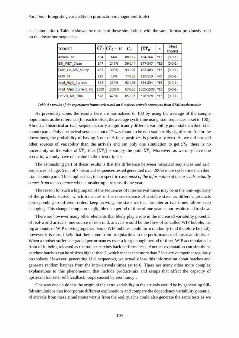
Part Two - Integrating variability (in production management tools)
104
each simulation). Table 4 shows the results of these simulations with the same format previously used
on the downtime sequences.
Table 4 : results of the experiment framework tested on 6 toolsets arrivals sequences from STMicroelectronics
As previously done, the results here are normalized to 100 by using the average of the sample
populations as the reference (for each toolset, the average cycle time using i.i.d. sequences is set to 100).
Almost all historical arrivals sequences carry a significantly different variability potential than their i.i.d.
counterparts. Only one arrival sequence out of 7 was found to be non-statistically significant. As for the
downtimes, the probability of having 5 out of 6 false-positives is practically zero. As we did not add
other sources of variability than the arrivals and ran only one simulation to get 𝐶𝑇̅̅̅̅0, there is no
uncertainty on the value of 𝐶𝑇̅̅̅̅0, thus [𝐶𝑇̅̅̅̅
0] is simply the point 𝐶𝑇̅̅̅̅0. Moreover, as we only have one
scenario, we only have one value in the t-test triplets.
The astonishing part of these results is that the difference between historical sequences and i.i.d.
sequences is huge: 5 out of 7 historical sequences tested generated over 200% more cycle time than their
i.i.d. counterparts. This implies that, in our specific case, most of the information of the arrivals actually
comes from the sequence when considering horizons of one year.
The reason for such a big impact of the sequences of inter-arrival times may be in the non-regularity
of the products started, which translates in the non-existence of a stable state: as different products
corresponding to different orders keep arriving, the statistics that the inter-arrival times follow keep
changing. This change being non-negligible on a period of time of one year as our results tend to show.
There are however many other elements that likely play a role in the increased variability potential
of real-world arrivals: one source of non i.i.d. arrivals would be the flow of so-called WIP bubble, i.e.
big amounts of WIP moving together. Some WIP bubbles could form randomly (and therefore be i.i.d),
however it is most likely that they come from irregularities in the performances of upstream toolsets.
When a toolset suffers degraded performances over a long-enough period of time, WIP accumulates in
front of it, being released as the toolset catches back performances. Another explanation can simply be
batches: batches can be of sizes higher than 2, which means that more than 2 lots arrive together regularly
on toolsets. However, generating i.i.d. sequences, we actually lose this information about batches and
generate random batches from the inter-arrivals times set to 0. There are many other more complex
explanations to this phenomenon, that include product-mix and setups that affect the capacity of
upstream toolsets, self-feedback loops caused by reentrancy…
One way one could test the origin of the extra variability in the arrivals would be by generating full-
fab simulations that incorporate different explanations and compare the dependency variability potential
of arrivals from these simulations versus from the reality. One could also generate the same tests as we
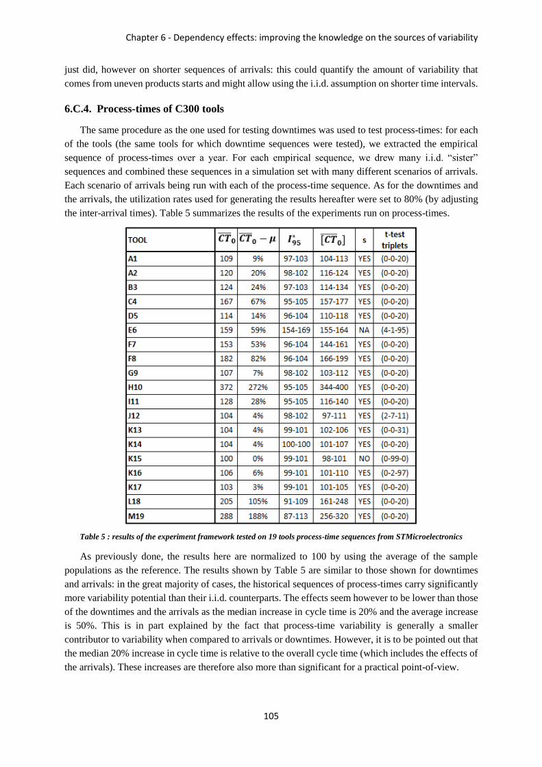
Chapter 6 - Dependency effects: improving the knowledge on the sources of variability
105
just did, however on shorter sequences of arrivals: this could quantify the amount of variability that
comes from uneven products starts and might allow using the i.i.d. assumption on shorter time intervals.
6.C.4. Process-times of C300 tools
The same procedure as the one used for testing downtimes was used to test process-times: for each
of the tools (the same tools for which downtime sequences were tested), we extracted the empirical
sequence of process-times over a year. For each empirical sequence, we drew many i.i.d. “sister”
sequences and combined these sequences in a simulation set with many different scenarios of arrivals.
Each scenario of arrivals being run with each of the process-time sequence. As for the downtimes and
the arrivals, the utilization rates used for generating the results hereafter were set to 80% (by adjusting
the inter-arrival times). Table 5 summarizes the results of the experiments run on process-times.
Table 5 : results of the experiment framework tested on 19 tools process-time sequences from STMicroelectronics
As previously done, the results here are normalized to 100 by using the average of the sample
populations as the reference. The results shown by Table 5 are similar to those shown for downtimes
and arrivals: in the great majority of cases, the historical sequences of process-times carry significantly
more variability potential than their i.i.d. counterparts. The effects seem however to be lower than those
of the downtimes and the arrivals as the median increase in cycle time is 20% and the average increase
is 50%. This is in part explained by the fact that process-time variability is generally a smaller
contributor to variability when compared to arrivals or downtimes. However, it is to be pointed out that
the median 20% increase in cycle time is relative to the overall cycle time (which includes the effects of
the arrivals). These increases are therefore also more than significant for a practical point-of-view.

Part Two - Integrating variability (in production management tools)
106
We can also notice from these results that the type of tool seems to play a significant role in the
variability potential stored in the sequence of process-times. Indeed, all tools from family K show very
similar results (even though one out of the 5 tools shows no statistically significant difference). We
however do not have enough results to fully assert this, but this could be a perspective for future studies.
One explanation to the origin of the dependent process-times might be common to the explanation
for the arrivals: the mix of products started shifts considerably over a year, and this shift in product-mix
changes the average process-times that the tools do. This cause can explain several of the big differences
in cycle times, but certainly does not explain everything. Indeed, the tools A1 and A2 have almost no
product-mix so their average process-time stayed constant over the period considered, however they
also show an increase dependency variability potential. For these tools, the health of the tools might be
the main contributors to the variability potential of their process-times. Indeed, as we had explained in
part 3.B.2 of this manuscript, some tools run on multiple chambers in parallel, and the failure of one
chamber does not necessarily trigger the failure of the mainframe, but if the mainframe continues
running, it processes lots with a degraded process-time. One way one could test further from where this
dependency variability potential comes from could be to have the process-times being random within a
recipe type, but having recipe types follow the sequence dictated by the historical sequence.
6.D. Conclusion and perspectives
6.D.1. Summary of the results
Accurate modelling of sources of variability (i.e. root causes for the generation of queuing time
inefficiencies) is a key element of the manufacturing strategies put forward with industry 4.0 and High
Mix Low Volume production. Previous works had questioned the viability of the assumption of
independent and identically distributed random variables when it comes to the modelling of sources of
variability such as tool downtimes, arrivals, process-times…
In this section, we first proposed an experiment framework based on the repetition of many
simulation runs that allows testing on historical sequences of data if this assumption has any implication
in the modelling of variability. The experiment framework was built around the specific scenario of
testing downtimes, but can be applied to any sequence of data as long as a simulation is able to
incorporate the source of variability that is tested.
We then tested 19 different industrial downtime sequences of 1 year taken from tools from the
Crolles 300 semiconductor fab, as well as process-time sequences over one year of the same tools and
arrivals sequences on 7 different toolsets. The results show that not only do the historical sequences
carry significant variability potential, they actually contain most of the variability potential. We also
showed that, quite interestingly, the sequences of downtimes can actually carry negative variability
potential and generate less cycle time than if they were sequences of independent and identically
distributed variables, an information that might come useful for running variability reduction programs.
6.D.2. A necessary correlation
The results we show indicate that most of the cycle time generated by downtime events and arrivals
from historical data is unaccounted for in most queuing theories and simulations. However, the
difference in cycle times between most current models (using queuing theory or simulation) and reality
is not in the order of magnitude that we pointed out. How can it be that we see a significant difference
that does not happen in reality?

Chapter 6 - Dependency effects: improving the knowledge on the sources of variability
107
We believe this difference comes from another dependency phenomenon that is still mostly
unaccounted for: the dependency between the arrivals and the tool behaviors. Indeed, in the complex
reality of manufacturing, decisions are made dynamically based on the flow of products. For instance,
maintenances might be pushed back in the case of temporary over-saturations, more maintenance staff
is also affected to tools that are forecasted to be highly used in the near future, etc… There is therefore
strong clues that there is a correlation between arrivals and tools downtimes that is not yet accounted.
This correlation might be a key both to modelling and to improving performances of real-life
manufacturing systems: indeed, if it can be measured, followed and encouraged, this correlation can
become a strong lever to decrease workflow variability. In this sense, we should first increase the
research in the ability of WIP forecasts to predict significant variations in the arrivals which we just
showed is not random (such as the prediction of WIP bubbles or differences in medium run saturations).
We should then be able to measure this correlation, i.e. measure the synchronization between the
performances of the toolsets and the arrivals at these toolsets, the objective being to have best
performances when these are required. We should then push for preventive actions aiming at increasing
this correlation (for instance managing maintenances or engineering activities in order for them to
happen when the capacity of the toolsets are the least required).
6.D.3. Closing the gap between academics and industrials: a new era for modelling
Entering the new era of Industry 4.0 where the data is fully accessible and the computation capacities
allow powerful simulations, we cannot keep the same modelling techniques as a century ago. Complex
manufacturing systems such as High Mix Low Volume production facilities have an unprecedented
level of complexity, translated in the high levels of workflow variability and the density of information
that the sources of variability carry.
This new complexity can be dealt with. It however requires a meticulous dissection of the different
components that create it (the sources of variability), to understand how they act on the system and how
they add variability separately and when combined. As each system is different and the amount of
combinations is unconceivable, we need to understand the different aspects of each source of variability
and to model the different impacts based on complex measures such as through simulations. Indeed,
models built with a bottom/up approach are unlikely to integrate all the specificities and the complexities
of the system. However, measuring some aggregated aspects, such as the dependency variability
potential, or the effects of product-mix in a given flexibility configuration, and incorporating those
measures into upper-level models could produce good results.
In order to achieve such levels of close relations between the physical systems and the models, there
needs to be closer relations between the model providers and the “system providers”, i.e. between the
academics and the practitioners. Closing the gap between the academics and the industrials is one of the
key aspects of Industry 4.0, which will allow industries to better model their variability and push up
their productivity as they move towards High Mix Low Volume production, allowing a new era of
manufacturing in Europe.


Chapter 6 - Dependency effects: improving the knowledge on the sources of variability
109
Part Three
III Towards variability
reduction
Part One of this manuscript explained in-depth what workflow variability is, why it is important,
and gave tools and methods to accurately measure it. Part Two then focused on integrating variability
in production management tools. First through a direct integration of the cycle time consequences in
WIP projection tools, effectively allowing a better tractability of the manufacturing system. Secondly
through better measures of the actual performances of process-clusters (toolsets) using newly introduced
tools and notions, therefore allowing the derivation of models that integrate more aspects of workflow
variability. Finally, we explained that integrating variability also goes through a better understanding of
what creates workflow variability in real life, and focused our attention on dependency effects which
we showed plays a great role in the generation of workflow variability.
The most challenging objective however, the saint grail of manufacturing, is to achieve sustainable
and continuous variability reduction. Reducing workflow variability would indeed mean shifting from
curative firefighting strategies to sustainable preventive actions, allowing to drastically decrease cycle
times (and therefore gain effective capacity) and increase the systems tractability. Part Three of this
manuscript explores the required steps to achieve such variability reduction. We first discuss (chapter 7)
the potential of simulation tools to increase our knowledge on the mechanisms of workflow variability
and to pinpoint where actions need to be taken to reduce workflow variability. We indeed show the
perspectives we see in improving simulation models using feedback from real data to identify the root
causes effectively responsible for workflow variability.
We then focus on more global perspectives in chapter 8: we explain the potential that we see in
studying the global aspects of workflow variability through full-fab simulations, and explain the
different steps that we believe need to be checklisted to achieve that. We then, in the second part of
chapter 8, unroll our vision, based on the literature and our experience, for a plan to achieve variability
reduction in a complex manufacturing environment with works and results expected from a 1 year
horizon to a 10 year horizon.
.


Chapter 7 - A plan to identify variability reduction levers (using simulation)
111
Chapter 7
7. A plan to identify variability
reduction levers (using simulation)
The first two parts of this manuscript focused on the identification, measure, and integration of
variability, which leads to a better tractability of the system by integrating this knowledge into the
different production management tools. The saint grail however is to be able to reduce workflow
variability, as this reduction automatically leads to both an enhanced tractability of the system and
improved cycle times. Thus, the aim of Chapter 7 is to propose a structured framework that will allow
identifying key levers on which actions can be taken in order to reduce workflow variability.
The first aspect of the plan is to find where the workflow variability is, using the measurement tools
proposed in chapter 2. The next milestone is to replicate, using a simulation model, the exact same
workload profile (see chapter 2) that happened in reality on the targeted process-clusters. The objective
then being to tweak the simulation model as to find what could have been done differently in the past to
reduce workflow variability.
We focus in this chapter on the elements that we believe are necessary to unroll such a plan: first,
the better we understand how each individual source of variability works, the better our overall
understanding (and ability to find levers) gets; so the continuous improvement on the knowledge of
individual sources of variability is compulsory. Similarly, as we have only scratched the surface on the
correlations and influential effects between different sources of variability and as there is strong
evidence that these play a major role in the generation of workflow variability, further studying these
combined effects is another no-brainer. We therefore start by describing the essential elements we
believe should be further studied when it comes to studying individual sources of variability and
dependency phenomenon. Moreover, replicating historical workload profiles is inherently difficult for
complex systems as there are many un-modelled small sources of variability which end up having big
consequences in real life: we will therefore propose an innovative approach that allows improving the
modelling of past events using feedbacks from the reality as to establish the best simulation model from
the available information. Finally, we show, through a test-case study of a process-cluster of the C300
fab, how we believe, once the previous milestones are reached, our framework can be articulated to
“zero in” on the main sources of variability and key levers.
.

Part Three - Towards variability reduction
112
7.A. Master plan: study the past to change the future
Using the different tools and knowledge presented in this manuscript, the objective of this chapter
is to show how reducing workflow variability is possible on the short term, and which aspects need to
by studied or further improved to do so.
In order to effectively reduce workflow variability, we propose to first act where there is the most
workflow variability through a Pareto approach. In order to do so, one would need to divide the
manufacturing system into process-clusters (and ideally, into highly connected process-cluster, see
section 2.E.2), measure the amount of workflow variability at each of those using the measures proposed
in section 2.D, and act on the workflow variability one process-cluster after another in a continuous
improvement logic, starting with the most problematic process-clusters.
Once a process-cluster has been identified as a candidate for reducing its workflow variability, we
will want, somehow, to know which levers can be used to reduce the workflow variability at this process-
cluster. The general idea is to found out which levers could have been acted on in the past to reduce the
workflow variability in the past. By doing so, we infer that the sources of variability from the past will
keep acting in the future. In order to find out the possible levers of past events, we propose developing
simulation models that are able to reproduce the exact same workload profile (see chapter 2) as happened
on the real-life process-cluster. If the replication is achieved with a sufficient precision, this means that
the simulation model contains all the information needed to understand what created the workflow
variability (in this specific period from the past). From there, we can tweak the simulation model
(operate slight changes in the model inputs) and study the impact different changes would have had on
the past as to narrow down on which inputs are the most impactful (which are effectively the main
sources of variability) and which changes can bring down the workflow variability.
This aforementioned framework is the general concept which we would like to unroll as to allow
effectively starting variability reduction. This framework however requires a few essential elements as
to unroll properly: first, as our objective is to simulate changes in the past events, we can only change
sources of variability and action mechanisms that we have properly understood. In order to have a wide
range of possible levers, we therefore need a wide range of controlled inputs, which means we need to
further understand how each source of variability acts on the system to create workflow variability. For
instance, as we have showed the impact of dependencies on workflow variability, the more we
understand about the dependencies and the more we are able to replicate them, the more levers we will
have access to. Parts 7.B and 7.C discuss the improvements that can be made to model the mechanisms
of variability.
Moreover, creating a simulation model which recreates the exact same workload profiles as in the
past seems complicated as modelling each and every source of variability and each interaction is almost
impossible and would consume tremendous resources. What we propose is therefore to build simulation
models using a feedback loop on the reality to fit a “residual function”. By doing so, we can incorporate
the main workload fluctuations in the primary sources of variability that are individually modelled, and
incorporate all other otherwise unaccounted sources of variability and interactions in the residual
function. The idea behind doing this is that the main components, the ones individually modelled, should
be responsible for the main variations, whereas the other components on the other hand should have a
rather stable aggregated impact. Part 7.D shows exploratory work in this direction, and finally part 7.E
shows an example of root cause analysis on the fitted simulation, along with analysis which guide us on
main levers to act on.

Chapter 7 - A plan to identify variability reduction levers (using simulation)
113
7.B. Improving knowledge on individual sources of variability
7.B.1. The necessity of a full understanding
The actions we take on a real system can only be as good as our understanding of this system. In
order to address variability, it is therefore compulsory to understand, with the highest precision, not only
what creates variability, but also how each component acts and increases this variability. As we have
listed in the first part of this manuscript the twenty sources of variability that are commonly agreed to
be the most impactful, we believe each source of variability should be addressed in-depth as to
understand the mechanisms that make this source of variability impactful. As explained is chapter 3, a
lot of work has focused on tool redundancy, downtimes, and process-time. However, these sources of
variability are far from being sufficient to model complex process-clusters such as find in typical HMLV
fabs. In order to accurately model variability and identify the major levers, the models need to
incorporate other impactful sources such as tool dedication, product-mix, batches, setups, dispatching
policies… To do so, it is also compulsory to understand how each of these acts, what are the
characteristics that act on the system in theory AND in reality. This section (7.B) highlights the factors
that we believe should be studied first and the mechanisms we should be able to model.
7.B.2. The non-linear capacity of complex process-clusters
Setups and batches: complexifying capacity
As explained previously (see e.g. chapter 5), the capacity of the system is a parameter found in many
models, which seems pretty obvious as the capacity is unarguably the most important characteristic of
a process-cluster. However, defining the capacity infers that the capacity is a constant parameter in a
system, a fixed element. As previously mentioned, complex processes, such as those find in
microelectronics, do not obey this fixed capacity rule. Setups, for instance, describe an additional fixed
time needed to switch from one job-family (or recipe) to another; and this extra source of inefficiency
is not a constant: if there is more WIP in front of the process-units, there is on average more of the same
job-family in that WIP (waiting to be processed), and there is therefore a higher chance of processing
more of the same job-family in a row before having to switch to another job-family (and perform a
setup). As the setups only occurs when switching from one job-family to another, a higher WIP level
will decrease the number of setups and thus result in a higher capacity. The reasoning is the same for
batches: the higher the WIP, the higher the likelihood of performing full batches, and the higher the
capacity. This non-linear relation has a surprising effect that we can describe as a “positive stable WIP
level”, i.e. in the absence of variability, a stable system with a non-linear capacity will constantly have
some WIP waiting to be processed, whereas a stable fixed capacity system will have no WIP waiting in
the absence of variability. To be exact, this phenomenon will happen at any process-cluster with non-
linear capacity for which the arrival rate is higher than the minimum capacity but lower than the
maximum capacity. Indeed, for such process-clusters, if the WIP level is low, the capacity (and therefore
the throughput) will be smaller than the arrival rate, and the WIP will therefore increase. However, as
this WIP increases, so does the capacity. Therefore, once this WIP level is high enough, the throughput
will be greater than the arrival rate, and the WIP level will stabilize. This will then result in a stable
workload level around which the workload will fluctuate. We can see this effect quite straightforwardly
on real industrial data. Figure 42, for instance, shows the evolution of the workload in front of a toolset
of the C300 fab: this workload varies, but generally stabilizes around a workload of 3 hours of waiting
time.

Part Three - Towards variability reduction
114
Figure 42: evolution of workload waiting at a toolset of C300 fab.
The impact of product-mix
The setups and incomplete batches are sources of variability by themselves, but they are also the
result of other sources, that can effectively increase the number of setups and of incomplete batches.
One such source, as explained earlier, is product-mix. Indeed, the higher the product-mix, the smaller
the amount of identical job-families are in a queue of a given length, and therefore, the more
inefficiencies (setups or incomplete batches) are produced. Figure 43 illustrates this problem.
Figure 43: the effect of increased product-mix on process-clusters with setups or batches
Figure 43 shows the non-linear relation between the throughput (capacity) of a process-cluster and
the workload at this process-cluster. For any product-mix, the throughput increases as the workload
queuing increases (as we explained in the previous paragraph). Figure 43 also shows that, for any
product-mix, a process-cluster with a non-linear capacity (e.g. setups) will experience a stable WIP level
(shown as well by Figure 42). However, the higher the product-mix is, the fewer identical products can
be found for a given WIP level, and therefore the more switching between different job-families is

Chapter 7 - A plan to identify variability reduction levers (using simulation)
115
required, i.e. the more setups are required, which means a decreased throughput. This is what the
different curves of Figure 43 explain: the higher the product-mix, the lower the throughput curve.
The impactful consequence of this is that the higher the product-mix is, the higher the stable WIP
level becomes. This has consequences on all aspects of workflow variability: first, the cycle times are
higher since the queues are longer, but a higher mean also means a higher variance, i.e. absolute
uncertainty in the level of workload (which overall means increased workflow variability).
7.B.3. The impact of operational factors
As discussed in chapter 2, operational factors are the factors related to decisions and actions we take
on the system. As so, these factors are the ones with the highest short term potential as their changes
require no physical investment and can therefore be implemented at low cost and in a rapid manner. For
instance, the scheduling policies and algorithms used have a great influence on the impact the product-
mix has on setups and incomplete batches, and thus on variability. As these are the most direct levers
available to decrease variability, it is essential to fundamentally understand how these factors affects the
variability and to be able to quantify the effects in different settings.
7.B.4. Understanding fundamental properties through simulation
In order to integrate the aforementioned phenomenon in simulation models to a point where they
can be used as levers, it is necessary to gather knowledge on each of these sources of variability.
Simulation is a promising tool for this: as we can control the varying parameters, we can, through
simulation, run many experiments which will be targeted (for instance) at the following questions: how
big of an impact does the product-mix have on variability? Can we estimate the “variability potential”
of a specific product-mix? How big of an impact do the operational factors have on different
configurations?
These simulations, as they will help the general understanding of variability, can also be organized
in a way that brings straight answers to current problems. For instance, testing different scheduling
algorithms or batch rules through simulation will not only bring useful insights on the variability this
operational factor brings, it will also allow to choose methodologically which rule or schedule policy
should be used in specific conditions.
7.C. Modelling of dependencies
7.C.1. Modelling dependencies for individual sources
The importance of dependencies
As we have shown in chapter 6 dependencies can play an extremely important role in the workflow
variability that process-clusters experience. In the semiconductor HMLV fab of Crolles 300, dependent
behaviors have a huge “variability potential”: we indeed showed for several sources of variability that
using the historical (dependent) sequence of events in a simulation instead of an independent sequence
resulted in much higher cycle times. For instance, downtimes for the tools we tested in chapter 5 follow
dependent sequences, with a resulting cycle time significantly different than if they were independent.
It is therefore necessary to increase the knowledge we have about these behaviors as to understand what
in these behaviors has potential to increase or decrease workflow variability, what elements are
responsible for these dependencies and how we can have more tractability on it. A first step towards a

Part Three - Towards variability reduction
116
deeper understanding would be to be able to model them, i.e. to have the ability to generate sequences
of events that have the same characteristics and more importantly the same consequences. This section
therefore sets the different perspectives we see in the modelling of dependencies, and the way we would
further study these elements.
Possible options for modelling dependencies
The most obvious way to generate dependent sequences of data with a level of dependency that
corresponds to the one observed in reality would be through the understanding and quantification of this
dependency. One fundamental aspect of this understanding would go through looking at the sequences
of data at different scales: indeed, some dependencies might be very local (e.g. downtimes can be likely
to come by close pairs) while others can be very global (e.g. some sequences of data can have monthly
variations in their downtimes). Whatever the procedure, it is fundamental to keep in mind that the
consequence is what we are interested in. For instance, if a mathematical test indicates that the level of
dependency in two sequences are identical, but the average cycle time generated with these sequences
through simulation are significantly different, then this test is not appropriate for our purpose.
Another way we can imagine generating dependent sequences that “mimic” the real-world
dependencies is by using a neural network whose mission would be to create sequences of data that yield
the same “variability potential” as the input sequence. LSTM networks [73] (Long Term Short Term
neural networks) are recognized as powerful tools for data generation with dependencies such as text
generation that resembles a given language [74]. Such neural network could be trained using
input/output data from simulations as we used in chapter 5. As we repeat the exact same simulation,
only with different input parameters, resulting in different output values, we could use the output cycle
time, the secondary inputs, as well as an i.i.d. sequence of the sequence that was tested in the simulation
as inputs of the neural network; and use the actual sequence of our simulation as the output of our neural
network for the training phase. The key element would be our ability to generate enough dependent
sequences as to train sufficiently well the neural network. This however could be achieved by applying
transformations to the historical sequences of data, as for the new sequences to be different than the
historical ones, but keep many of their characteristics as some of the dependencies.
7.C.2. Modelling interactions between different factors
Interactions between different sources of variability: the missing link
One of the conclusions of chapter 6 was the evidence supporting a strong level of interaction between
the different factors: for instance the behavior of the process-cluster (especially the downtimes) seem to
be strongly linked to the arrivals at the process-cluster. Following the objective of this chapter, which is
finding levers to decrease workflow variability, understanding these interactions (the origins, the effects,
etc.) would straightforwardly lead to more levers and better chances of achieving this objective.
Dependencies between process-units
As the different process-units in a process-cluster work together to treat an incoming flow of
products, it is common practice in real fabs to try and sync the different process-units as to not get all
process-units down at the same time. For instance, the preventive maintenances are (if possible) never
done on all tools at once, but are generally evenly spread. This introduces strong dependencies between
the downtimes of the different process-units of a process-cluster. As the goal is generally to reduce cycle
time, it is fair to assume that this dependency (which is introduced by strategic decision) also has a
significant impact on workflow variability and cycle time.
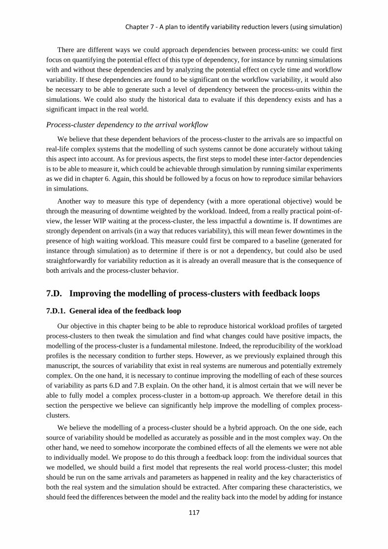
Chapter 7 - A plan to identify variability reduction levers (using simulation)
117
There are different ways we could approach dependencies between process-units: we could first
focus on quantifying the potential effect of this type of dependency, for instance by running simulations
with and without these dependencies and by analyzing the potential effect on cycle time and workflow
variability. If these dependencies are found to be significant on the workflow variability, it would also
be necessary to be able to generate such a level of dependency between the process-units within the
simulations. We could also study the historical data to evaluate if this dependency exists and has a
significant impact in the real world.
Process-cluster dependency to the arrival workflow
We believe that these dependent behaviors of the process-cluster to the arrivals are so impactful on
real-life complex systems that the modelling of such systems cannot be done accurately without taking
this aspect into account. As for previous aspects, the first steps to model these inter-factor dependencies
is to be able to measure it, which could be achievable through simulation by running similar experiments
as we did in chapter 6. Again, this should be followed by a focus on how to reproduce similar behaviors
in simulations.
Another way to measure this type of dependency (with a more operational objective) would be
through the measuring of downtime weighted by the workload. Indeed, from a really practical point-of-
view, the lesser WIP waiting at the process-cluster, the less impactful a downtime is. If downtimes are
strongly dependent on arrivals (in a way that reduces variability), this will mean fewer downtimes in the
presence of high waiting workload. This measure could first be compared to a baseline (generated for
instance through simulation) as to determine if there is or not a dependency, but could also be used
straightforwardly for variability reduction as it is already an overall measure that is the consequence of
both arrivals and the process-cluster behavior.
7.D. Improving the modelling of process-clusters with feedback loops
7.D.1. General idea of the feedback loop
Our objective in this chapter being to be able to reproduce historical workload profiles of targeted
process-clusters to then tweak the simulation and find what changes could have positive impacts, the
modelling of the process-cluster is a fundamental milestone. Indeed, the reproducibility of the workload
profiles is the necessary condition to further steps. However, as we previously explained through this
manuscript, the sources of variability that exist in real systems are numerous and potentially extremely
complex. On the one hand, it is necessary to continue improving the modelling of each of these sources
of variability as parts 6.D and 7.B explain. On the other hand, it is almost certain that we will never be
able to fully model a complex process-cluster in a bottom-up approach. We therefore detail in this
section the perspective we believe can significantly help improve the modelling of complex process-
clusters.
We believe the modelling of a process-cluster should be a hybrid approach. On the one side, each
source of variability should be modelled as accurately as possible and in the most complex way. On the
other hand, we need to somehow incorporate the combined effects of all the elements we were not able
to individually model. We propose to do this through a feedback loop: from the individual sources that
we modelled, we should build a first model that represents the real world process-cluster; this model
should be run on the same arrivals and parameters as happened in reality and the key characteristics of
both the real system and the simulation should be extracted. After comparing these characteristics, we
should feed the differences between the model and the reality back into the model by adding for instance
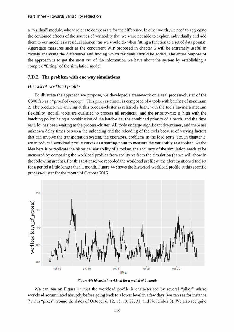
Part Three - Towards variability reduction
118
a “residual” module, whose role is to compensate for the difference. In other words, we need to aggregate
the combined effects of the sources of variability that we were not able to explain individually and add
them to our model as a residual element (as we would do when fitting a function to a set of data points).
Aggregate measures such as the concurrent WIP proposed in chapter 5 will be extremely useful in
closely analyzing the differences and finding which residuals should be added. The entire purpose of
the approach is to get the most out of the information we have about the system by establishing a
complex “fitting” of the simulation model.
7.D.2. The problem with one way simulations
Historical workload profile
To illustrate the approach we propose, we developed a framework on a real process-cluster of the
C300 fab as a “proof of concept”. This process-cluster is composed of 4 tools with batches of maximum
2. The product-mix arriving at this process-cluster is relatively high, with the tools having a medium
flexibility (not all tools are qualified to process all products), and the priority-mix is high with the
batching policy being a combination of the batch-size, the combined priority of a batch, and the time
each lot has been waiting at the process-cluster. All tools undergo significant downtimes, and there are
unknown delay times between the unloading and the reloading of the tools because of varying factors
that can involve the transportation system, the operators, problems in the load ports, etc. In chapter 2,
we introduced workload profile curves as a starting point to measure the variability at a toolset. As the
idea here is to replicate the historical variability of a toolset, the accuracy of the simulation needs to be
measured by comparing the workload profiles from reality vs from the simulation (as we will show in
the following graphs). For this test-case, we recorded the workload profile at the aforementioned toolset
for a period a little longer than 1 month. Figure 44 shows the historical workload profile at this specific
process-cluster for the month of October 2016.
Figure 44: historical workload for a period of 1 month
We can see on Figure 44 that the workload profile is characterized by several “pikes” where
workload accumulated abruptly before going back to a lower level in a few days (we can see for instance
7 main “pikes” around the dates of October 6, 12, 15, 19, 22, 31, and November 3). We also see quite
Chapter 7 - A plan to identify variability reduction levers (using simulation)
119
interestingly that the workload almost never reaches zero: the stable point is around 6 hours_of_process
(which is about 4 lots since the average process-time is around 1.5 hours). The pikes and the stable
workload level are basically what characterizes the workload profile of this process-cluster over this
period. Thus, the simulation model that we make of this process-cluster should be able to imitate those
as closely as possible.
Raw simulation model
We created a first simulation model for this toolset by identifying all the main sources of variability
and integrating them in the simulation: the simulation model includes the downtimes, batches, tools
qualifications, product-mix, priority-mix and the batch policy. As the objective is to replicate the
workload profile over a period of one month, we fed the simulation with the exact same arrivals as in
the reality and set the tools to undergo the same downtimes as in reality. The simulation gave as an
output the arrival-time and process-start-time of each lot, which we then used to build the workload
profile of the simulated toolset. Figure 45 shows the workload profile we obtained through this
simulation compared to the historical workload profile (in the background). Having both curves in the
same graph allows a careful comparison of the outputs of the simulation vs the reality.
Figure 45 : workload profile from the raw simulation compared to the historical profile
As we can observe on Figure 45, the two characteristics from our previous workload profile could
be improved: apart from the pike around October 6, the other workload pikes are far from being
modelled correctly in our simulation model as they are barely noticeable in the simulation. Moreover,
we can see in Figure 45 that the stable workload of our simulation is almost at zero, when it was around
6 hours-of-process in reality.

Part Three - Towards variability reduction
120
7.D.3. The feedback loop: a “residual function” to fit the simulation
The impact from secondary sources of variability
As we explained through this manuscript, the reality is extremely complex and is made of many
(many) different sources of variability that all interact with each other in order to create the output which
we can measure as the workload profile. Therefore, even though we included all the major sources of
variability of the process-cluster in the model, we end-up having a simulation that is not representative
of the reality. The reason being that the small sources of variability have a combined effect that is non-
negligible. However, we can see on Figure 45 that the main variations seem to be correctly modelled:
all the pikes from the historical curve (grey) seem to exist in the simulation model (black), just being
often much fainter. We can therefore assume (with the same reasoning logic as we had in chapter 4 when
we built the cycle time model) that the impact of the “other” sources of variability (the ones we have
not been able to include in our model) does not create major variations but acts more as a background
noise, i.e. a background impact on the capacity of the system. The idea is the same as fitting a regression
model on a system where there are 30 actual variables but with only the 4 or 5 main ones with available
data: the residual of the regression will contain the combined effects of the other 25 variables, and is
generally different than 0. From the explanations in 7.B.2, we can also assume that more inefficiencies
should increase the stable WIP to get something closer from the reality.
By analyzing the characteristics of both systems, and specifically aggregated characteristics, we
should be able to measure the “residual” between the reality and our simulation, and feed this residual
back into the simulation by adding a “residual inefficiency module” to our simulation. Note that this
“residual” does not need to be a constant: we have for instance explained at many occasions during this
manuscript that the capacity of the system depends on the workload for many reasons. We have included
a few of these in our simulation (through the historical downtimes and the batches combined with
product-mix), but we have not included all possible factors. It is likely that other sources of variability
can generate capacity-workload dependencies that we have not modelled. For instance, loading and
unloading partly depend on manual intervention, and as production teams have to deal with different
process-clusters at once (which can be far apart from one another in the manufacturing system), they
usually focus their attention on the highly loaded process-clusters, thus creating less inefficiencies on
highly loaded process-clusters.
Measuring the quality of the simulation and the direction of improvement
We cannot fit the residual as easily an in a regression since a simulation model is not a simple
equation where the numbers can move from one side of the equation to another. However the
fundamentals stay true: if the simulation has a workload inferior to that of the reality (as it is the case in
our example), we can reason that the average capacity of the simulation is higher than in reality and
should be decreased. In order to be more precise though, a few components are required: first, we need
to have a mathematical measure of the quality of the simulation as to be able to tell which simulation is
closest from the reality. Secondly, we need to be able to measure the direction of the difference, as to
know how the simulation should be changed as to improve it.
The measure we chose to evaluate the quality of the simulation is the relative difference in the
workload curves. This measure is done by first taking the area of the absolute difference in the workload
profiles of both curves (the real one and the simulated one), and dividing this area by the area under the
curve of the real workload profile: this gives us the percentage of the real workload profile that we were
unable to replicate in the simulation. The smaller the relative difference, the higher the quality of the

Chapter 7 - A plan to identify variability reduction levers (using simulation)
121
simulation model (for our specific purpose of reproducing what happened in reality). When applying
this measure to the raw simulation model of Figure 45, we get a value of 48%. This value means that
the absolute area between the real and the simulation workload is equal to 48% the area of the real
workload curve. When fitting the simulation model, our objective is to decrease this difference as much
as possible.
The residual fitting function
As our test case is mainly intended as a “proof-of-concept”, we chose a rather simple “residual
inefficiency module”: the module simply artificially increases the process-time of all lots following a
“residual function”. In this test-case, the residual function is also rather simple: it is a fixed time that has
a given value E1 under a workload threshold W1, and a second value E2 over this threshold. This means
that the processes in our simulation will see an E1 increase in their process-time if the current waiting
workload in the simulation is less than the threshold workload W1, and an increase of E2 if the current
waiting workload in the simulation is greater than W1. The “regression” of the values E1, E2 and W1
was done iteratively by analyzing the differences between the workloads of the successive simulations
to the reality: if at a workload lower than W1 the average workload in the simulation is lower than that
of the reality, E1 needs to be increased (or decreased otherwise). E2 can be fitted the same way, and W1
can be fitted by local search. We could have also added inefficiencies by simulating extra downtimes or
adding a blocking element in front of the toolset, we however chose to act on the process-times to follow
the reasoning of “Effective Process-Times” proposed by [12] and further studied by [20].
A significant improvement in the simulation
Figure 46 shows the workload profile of the simulation with this feedback loop compared to the
historical profile. As we can see in Figure 46, most historical workload pikes are well modelled by the
simulation.
Figure 46 : workload profile from the fitted simulation compared to the historical profile
Part Three - Towards variability reduction
122
Moreover, we have non-zero stable workload, though not quite as obvious as in the reality. When
applying our previous measure (the relative difference between both curves), we now measure a
difference of 36% between both curves. Compared to the original difference of 48% (Figure 45), we
managed to increase the quality of our simulation model by 25% [(48-36)/48] by adding a very simple
fitting function. There is still however a 36% difference between the simulation and the reality, which
could be reduced by either adding more explanatory variables or improving our fitting method. One
explanatory variable that we did not consider here and might actually impact our workload curves are
“hold” events. Indeed, lots can be put in “hold” for long periods of time, arbitrarily retaining workload
and potentially affecting the modelling. We emphasize that a 36% difference between two curves
actually translates a rather good fit in our case. Indeed, with our metric, the difference can get higher
that 100% (with asynchronous curves for instance).
7.D.4. Optimizing the feedback process
Although the previously described method allowed us to achieve a simulation that resembles reality
to a satisfactory point (the two curves in Figure 46), we believe many improvements can be brought to
the feedback loop process in order to get the best possible simulation model out of the available data
with relatively small resource investments. For instance, the residual function we chose for our
simulation model is extremely basic and was chosen for its ease of implementation. The choice of this
function, which can be continuous or by step as we did (but with a greater number of steps) as well as
the optimization method to find the best parameters can become a central aspect in the modelling of
complex process-clusters. Indeed, if it is done correctly, this process could significantly reduce the
development required to accurately model a process-cluster by making best (automatic) use of the
available information about the system. We strongly believe that aggregate performance measures (such
as those the concurrent WIP can provide) can be a key in finding the best residual function and
parameters for developing accurate models.
Another improvement to this feedback process can be the measure of “closeliness” that we used.
We chose to measure the absolute difference between two curves, as we believe this measure comes
with a meaning that is easily understandable. However, we could have also chosen to minimize the
square of the differences to get a measure closer from the ones used to fit regression functions.
7.D.5. Perspectives for simulations used in projections
We developed simulations with feedback loops in order to be able to reproduce past events with
retrospective simulations, in the perspective of running root cause analysis on the historical workflow
variability. As this example is used as means of illustrating perspectives, we strongly believe that this
process has the potential to develop accurate simulation models to be used for root cause analysis at a
low engineering cost.
However, this type of simulation fitting could also be used for simulations used in the case of
projections. In this later case, one requirement to verify would be that the residual function that was
optimized on a given time period holds effective on the next time periods (in other words, are the
combined effects of other sources of variability relatively constant in time?). This could be done by
training and testing the system the same way a neural network is trained: we would split the past horizon
(on which we have recorded all the data) into sections, fit the residual function on one section and test
it on the following sections. The objective in this case would be to get a type of residual function that is
robust in time, which is a slightly different objective than the one we had in our example.

Chapter 7 - A plan to identify variability reduction levers (using simulation)
123
7.E. Root cause analysis through simulation
7.E.1. General idea: changing inputs to understand their impact
Once we have successfully simulated a process-cluster as to get the same workload profile from the
simulation as from the reality (or close enough), we know that the simulation model contains all the
important factors which created the workload variations on the period of interest. Therefore, we know
that we have all the basic information to explain the workflow variability from that period. In other
words, we can now work outside of the reality, in our simulation environment.
However, we do not know which factors are the most important ones, and how the factors are linked
one to another as to create the workload profiles. The idea from there is therefore to change the
simulation inputs, one parameter at a time, and obverse and measure the differences created in the
outputs, as to understand which events are responsible for which parts of the workload profiles. For our
proof-of-concept, we will do exactly this on the simulation model we developed with the help of a
feedback loop. Throughout this section, we can now compare any tweaked simulation to the simulation
that was fitted to the reality (which we will call the original simulation). The objective of this section
being to provide a proof-of-concept for our idea of root cause analysis through simulations on historical
data, we will draw qualitative interpretations of the different simulations we will run, showing the
potential for deeper works.
Impact of downtimes and arrivals
As the commonly agreed most impactful factor on workflow variability is downtime events, one
first tweaked simulation that we can run is a simulation where the arrivals and all parameters are the
same, except for the downtimes. One option would be to keep all tools up through the entire simulation,
however this would change the downtime rate and therefore major other parameters such as the
utilization rate of the system. As what we wish to test here are the effects of the heterogeneity of the
downtimes (and only that), we cannot just simply put all tools “up”: we need to remove the variability
from downtime events without changing the long-run capacity of the system (i.e. the utilization rate).
One way of doing this is by reducing downtimes to totally regular microscopic down events: we can set
the tools to fall down for extremely short periods of time, evenly spread through the entire horizon. The
notion of “extremely short” is obviously relative, and actually depends on the order of magnitude of the
other events. We can therefore define “extremely short” here as being one order of magnitude smaller
than the other influential events. In our case, as the average process-time is around 1.5 hours and the
inter-arrival time is around 1 hour, downtimes of a few minutes can be considered “extremely short”.
We therefore set our downtimes to last 1 minute and to be separated by a fixed time (set as to have the
same overall downtime). We also set the simulation to have preemptive downtimes where the process
can continue after interruption, resulting in the downtimes effectively just increasing process-times, with
the variability of the downtime events being however totally erased. As the downtimes are the most
commonly agreed source of variability in our literature review, we expect the removal of downtime
variability in our simulation to significantly decrease the workload variability. By applying this
procedure to the previous example, we obtained the workload profile of Figure 47.

Part Three - Towards variability reduction
124
Figure 47 : workload profile from a simulation with historical arrivals, but no downtime variability
We can see from Figure 47 that, quite surprisingly, the removal of the downtime variability did not
have the expected results on the simulation: as the generally agreed main contributor to variability, we
would expect the workload variability to decrease once we removed downtime variability; however
what we see is that the workflow variability actually increased once we removed the downtime
variability (compared to the original simulation). We will show how complementary simulations can
provide a good explanation for the results of this simulation run.
The other explanatory variables being arrivals variability, product-mix and priority-mix associated
to batches, we can assume than some of these variables are responsible for the workflow variability of
the toolset that we see in the original simulation. To understand better what is happening, we ran another
simulation, this time turning back on the historical downtime events, however now removing completely
the arrivals variability (which we do by having a fixed inter-arrival time, set as for the number of arrivals
on the period to be identical to the original simulation). Note that the product-mix and priority-mix are
kept, as the order of arrivals and the information on each lot was kept. Figure 48 shows the workload
profile of this simulation. Note also that the y-axis of Figure 48 changed compared to those of the
previous workload profiles as this simulation generated a peak of workload much higher than on the
previous figures.
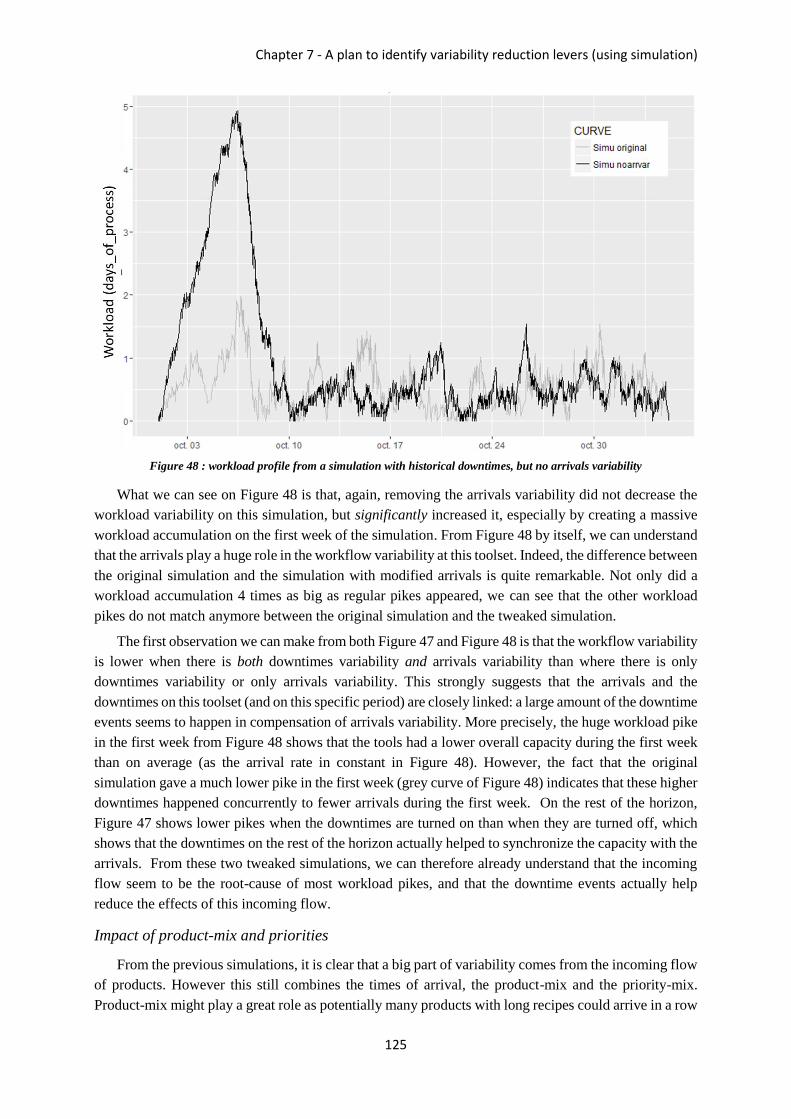
Chapter 7 - A plan to identify variability reduction levers (using simulation)
125
Figure 48 : workload profile from a simulation with historical downtimes, but no arrivals variability
What we can see on Figure 48 is that, again, removing the arrivals variability did not decrease the
workload variability on this simulation, but significantly increased it, especially by creating a massive
workload accumulation on the first week of the simulation. From Figure 48 by itself, we can understand
that the arrivals play a huge role in the workflow variability at this toolset. Indeed, the difference between
the original simulation and the simulation with modified arrivals is quite remarkable. Not only did a
workload accumulation 4 times as big as regular pikes appeared, we can see that the other workload
pikes do not match anymore between the original simulation and the tweaked simulation.
The first observation we can make from both Figure 47 and Figure 48 is that the workflow variability
is lower when there is both downtimes variability and arrivals variability than where there is only
downtimes variability or only arrivals variability. This strongly suggests that the arrivals and the
downtimes on this toolset (and on this specific period) are closely linked: a large amount of the downtime
events seems to happen in compensation of arrivals variability. More precisely, the huge workload pike
in the first week from Figure 48 shows that the tools had a lower overall capacity during the first week
than on average (as the arrival rate in constant in Figure 48). However, the fact that the original
simulation gave a much lower pike in the first week (grey curve of Figure 48) indicates that these higher
downtimes happened concurrently to fewer arrivals during the first week. On the rest of the horizon,
Figure 47 shows lower pikes when the downtimes are turned on than when they are turned off, which
shows that the downtimes on the rest of the horizon actually helped to synchronize the capacity with the
arrivals. From these two tweaked simulations, we can therefore already understand that the incoming
flow seem to be the root-cause of most workload pikes, and that the downtime events actually help
reduce the effects of this incoming flow.
Impact of product-mix and priorities
From the previous simulations, it is clear that a big part of variability comes from the incoming flow
of products. However this still combines the times of arrival, the product-mix and the priority-mix.
Product-mix might play a great role as potentially many products with long recipes could arrive in a row
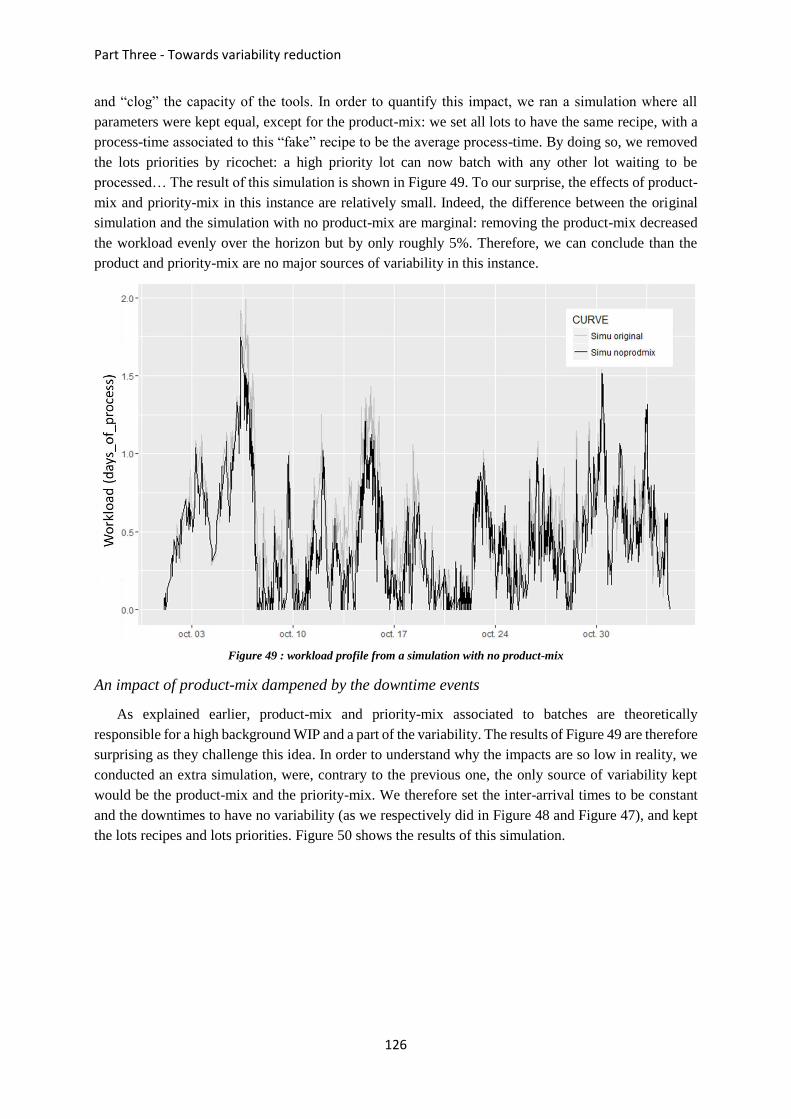
Part Three - Towards variability reduction
126
and “clog” the capacity of the tools. In order to quantify this impact, we ran a simulation where all
parameters were kept equal, except for the product-mix: we set all lots to have the same recipe, with a
process-time associated to this “fake” recipe to be the average process-time. By doing so, we removed
the lots priorities by ricochet: a high priority lot can now batch with any other lot waiting to be
processed… The result of this simulation is shown in Figure 49. To our surprise, the effects of product-
mix and priority-mix in this instance are relatively small. Indeed, the difference between the original
simulation and the simulation with no product-mix are marginal: removing the product-mix decreased
the workload evenly over the horizon but by only roughly 5%. Therefore, we can conclude than the
product and priority-mix are no major sources of variability in this instance.
Figure 49 : workload profile from a simulation with no product-mix
An impact of product-mix dampened by the downtime events
As explained earlier, product-mix and priority-mix associated to batches are theoretically
responsible for a high background WIP and a part of the variability. The results of Figure 49 are therefore
surprising as they challenge this idea. In order to understand why the impacts are so low in reality, we
conducted an extra simulation, were, contrary to the previous one, the only source of variability kept
would be the product-mix and the priority-mix. We therefore set the inter-arrival times to be constant
and the downtimes to have no variability (as we respectively did in Figure 48 and Figure 47), and kept
the lots recipes and lots priorities. Figure 50 shows the results of this simulation.
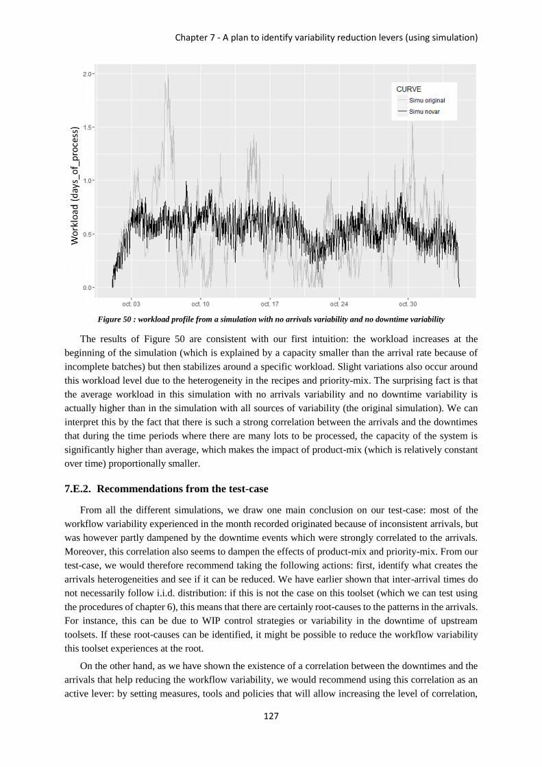
Chapter 7 - A plan to identify variability reduction levers (using simulation)
127
Figure 50 : workload profile from a simulation with no arrivals variability and no downtime variability
The results of Figure 50 are consistent with our first intuition: the workload increases at the
beginning of the simulation (which is explained by a capacity smaller than the arrival rate because of
incomplete batches) but then stabilizes around a specific workload. Slight variations also occur around
this workload level due to the heterogeneity in the recipes and priority-mix. The surprising fact is that
the average workload in this simulation with no arrivals variability and no downtime variability is
actually higher than in the simulation with all sources of variability (the original simulation). We can
interpret this by the fact that there is such a strong correlation between the arrivals and the downtimes
that during the time periods where there are many lots to be processed, the capacity of the system is
significantly higher than average, which makes the impact of product-mix (which is relatively constant
over time) proportionally smaller.
7.E.2. Recommendations from the test-case
From all the different simulations, we draw one main conclusion on our test-case: most of the
workflow variability experienced in the month recorded originated because of inconsistent arrivals, but
was however partly dampened by the downtime events which were strongly correlated to the arrivals.
Moreover, this correlation also seems to dampen the effects of product-mix and priority-mix. From our
test-case, we would therefore recommend taking the following actions: first, identify what creates the
arrivals heterogeneities and see if it can be reduced. We have earlier shown that inter-arrival times do
not necessarily follow i.i.d. distribution: if this is not the case on this toolset (which we can test using
the procedures of chapter 6), this means that there are certainly root-causes to the patterns in the arrivals.
For instance, this can be due to WIP control strategies or variability in the downtime of upstream
toolsets. If these root-causes can be identified, it might be possible to reduce the workflow variability
this toolset experiences at the root.
On the other hand, as we have shown the existence of a correlation between the downtimes and the
arrivals that help reducing the workflow variability, we would recommend using this correlation as an
active lever: by setting measures, tools and policies that will allow increasing the level of correlation,

Part Three - Towards variability reduction
128
we should be able to increase the efficiency of a currently informal control strategy, and therefore reduce
the workload variability at this toolset. In order to do so, we could for instance follow the “downtime
weighted by the workload”: indeed, downtime is only impactful if it has an impact on waiting workload.
By weighting the downtime by the workload, we would encourage freeing the capacity for when it is
useful, and encourage activities that generate downtime to occur during non-impactful time windows.
With this approach, we do not know yet how much the system can be improved with these actions.
The potential for improvement would be a very valuable information as it can justify (or not) an
investment of resources. Future research can therefore investigate the potential that correlated
downtimes can have on reducing workflow variability. A natural lower bound would be the variability
achieved when the tools are up 100 percent of the time: if the real situation is already close from the
lower bound, there is anyways not much improvement to do; otherwise, it is interesting to know how
much improvement we can reasonably expect.
7.F. Conclusion, perspectives and further research
7.F.1. A plan to reduce variability
The objective of this chapter was to show a path to variability reduction that uses simulations to
identify real-world levers to decrease workflow variability. We explored the different steps we identified
as crucial to do so and provided a test-case example to assert our reasoning.
The general idea of this “Master plan” is to model the past workflow variability in a simulation
model to then change various input parameters to identify the ones that can be used as levers to reduce
workflow variability, as well as identifying how these levers can be activated.
The first step of this plan being to be able to accurately model past workflow variability, accurate
modelling is necessary. In order to do so, we propose to incorporate individually the sources of
variability that are suspected to be main factors, while “fitting” the simulation to best describe reality
using feedback loops from the reality. We provided an exploratory example for such fitting as well as a
measure to evaluate the difference between the workload profiles of a simulation versus the reality. In
order to further enhance the power of these simulations to identify levers, we also believe that the
different sources of variability identified in chapter 3 should be studied in much higher detail than it is
currently the case as to understand exactly how these increase workflow variability in real-world
systems. In particular, we suspect that dependency effects such as those presented in chapter 6 play a
major role and that we should be able to correctly model those in order to incorporate them in the list of
available levers for variability reduction.
Once accurate modelling of past workflow variability is possible (and main factors are well
modelled), we believe sets of simulations with slight changes in the inputs can be used to identify main
levers for variability reduction. We provided a test-case on a toolset from the C300 fab of
STMicroelectronics and showed that it is possible, through simulation, to pinpoint the root causes of
workflow variability at a given process-cluster, with a clear direction to what actions should be taken in
order to reduce workflow variability. In our example, we have for instance put forward that the arrivals
were the main cause of workflow variability, and suggested investigating further the reason these
arrivals carried such variability potential. Furthermore, we pinpointed in this test-case that the
correlation (or synchronization) of downtimes was a major lever which is currently unofficially in use
and suggested pushing this approach by transforming it into a formal, measurable objective.

Chapter 7 - A plan to identify variability reduction levers (using simulation)
129
There is obviously lots of work to be done in this direction, as new results bring new questions. As
the example here was illustrative, we did not push the test-case further and relied a lot on interpretation
from the simulation curves. Further research in this direction should however provide a more
quantitative analysis and more direct conclusions. Nevertheless, we believe the guidelines we provided
in this section can be used as an engineering environment to start a sustainable process of variability
reduction.
7.F.2. Perspectives for research
As we pointed out the correlation of downtimes to arrivals as a main lever to reduce variability in
the test-case we provided, an interesting question arises: does knowing information about the future
arrivals significantly improves the potential of this lever? Indeed, knowing future arrivals can help us to
push backwards maintenances, do early maintenances, or move in time engineering actions on the
toolsets. In this context, it can be interesting to know how valuable the information from future arrivals
is: for instance, if we know exactly what will arrive in the future, how much can we reduce workflow
variability by acting on downtimes? We could answer this question by running numerous simulations
with the exact same arrivals with the objective of minimizing workflow variability by acting on the
sequence of downtimes. This would show the maximum potential one could expect from this lever.
On the other side of the spectrum, one could also ask how much information about the future is
required to implement strategies based on forecasts. Indeed, we will never know in practice the exact
arrivals from the future. However, can knowing approximately how many arrivals will occur on a given
horizon in the future be used to implement some strategies? If yes, how much information is needed?
And with a given amount of information about the future, how much variability reduction can we expect
by acting on the sequence of downtimes? We believe answering these questions would help direct
companies towards personalized mid-term and long-term research trajectories towards the objective of
reducing workflow variability.


131
Chapter 8
8. Further perspectives for
variability reduction
Chapter 7 covered the perspectives we see in using simulations to identify levers to reduce locally
workflow variability. Through a structures framework; we showed the different steps required to start
the process of variability reduction.
This chapter shows further perspectives for variability reduction. More precisely, we focus now on
a much larger time scale, allowing us to think about more ambitious and global approaches. We therefore
first show what we mean by a “global approach” to study variability, putting forward that local actions
can have global consequences as workflow variability can spread through a manufacturing system. We
show different works from the literature which investigate this global aspect of variability and emphasize
the potential we see in full scale simulations to fully address matters of workflow variability.
Finally, based on all the work presented in this manuscript, we put forward our vision for managing
workflow variability in a complex manufacturing environment on a very large time scale. Indeed, we
believe it is necessary to set a long term framework, as only paving progressively the different
milestones in the same direction will allow us to sustainably move forward. This is however only
realistic if each step also brings with it short-term results. We therefore show the different important
steps to progressively and continuously model and reduce workflow variability in manufacturing
systems on a horizon up to 10 years, from unrolling local variability reduction, to progressively
improving the modelling of the different sources of variability, to transitioning to more global simulation
models allowing more impactful actions. In order to do so in a sustainable manner, we also discuss the
different elements in a company we believe are essential to structure in parallel to the research: the
creation of a dedicated central team, the development of central and operational Key Performance
Indicators (KPIs*), and the involvement of the different teams in the company for a common objective
of improving the productivity and tractability of the entire manufacturing system.
Part Three - Towards variability reduction
132
8.A. Investigating variability on a global scale
8.A.1. The global nature of variability
Arrivals at process-clusters: the meeting point from other process-clusters
Through this manuscript, we generously discussed about the arriving workflow, and how the
heterogeneity in the inter-arrival times contribute greatly to workflow variability. Our results from
chapter 6 and chapter 7 actually suggest that most the workflow variability we measure at a process-
cluster originates from this incoming flow. Even though, as we have shown in chapter 7, levers can be
activated to reduce the effects of the arriving workflow, the next step is to understand how this arriving
workflow gathered so much variability potential in the first place, to then act on these root causes. As
the arriving workflow at a process-cluster is the combination of several upstream flows coming from
different upstream process-clusters, studying this arriving workflow means considering more than one
process-cluster at a time, i.e. a first step to a global approach.
Moreover, it is not necessarily where there is the most workflow variability that there is the more
potential to reduce the workflow variability. Indeed, as we showed for instance in chapter 7 that we can
use a better correlation of downtimes to arrivals in order to reduce the workflow variability, there might
be some process-clusters with a much higher potential to use this lever than others, even though their
workflow variability might be slightly lower. What this means is that, on the long term, it might be
interesting to consider the return on investment of different actions to take, and therefore to consider
several process-clusters in parallel in a more global approach.
Finally, the same way an arriving workflow at a process-cluster is a combination of different flows
from different process-cluster, an individual process-cluster actually downstreams workflow to many
different process-clusters. A complementary (and much more long term) approach to the one proposed
in chapter 7 is therefore to consider the sum of the effects specific actions (on a single process-cluster)
can have. These can include studying process-clusters with high reentrancy which might influence their
own arrivals through the reentrancy, but also studying process-clusters that have fewer arrival streams
(i.e. who receive jobs from fewer process-clusters) which may be more sensitive to upstream process-
cluster capacity losses than process-clusters with many arrival streams. We can also think about studying
the process-clusters that perform the early-stage processes, which might have bigger global impacts as
the flow that passes through these process-clusters can ripple through the entire manufacturing system
more easily…
Global reasoning: a long term objective
The local continuous improvement reasoning that we presented in chapter 7 is a necessary first step
to act on workflow variability, which is implementable on a short temporal horizon. In parallel to doing
so, it is equally important to think about the best way to deal with workflow variability. With the global
consequences that local actions can have, it is rather clear that the “optimal” approach is one that takes
into account the global consequences of actions. The long-term planning to dealing with workflow
variability should therefore converge towards a global approach. In the second section of this chapter,
we show how we believe the different elements of research and structures in a company can be arranged
as to lead to a global picture when considering workflow variability.
Chapter 8 - Further perspectives for variability reduction
133
8.A.2. Literature on global approaches to workflow variability
Several authors have directly or indirectly proposed ideas to approach globally workflow variability.
For instance, Wu [28] gives a formula for measuring the variability of a fab at a specific utilization rate,
based on the G/G/1 queuing formula. He also gives several formulas that link the variability of the fab
to characteristics of process-clusters of that fab, deriving several interesting conclusions: for instance,
he concludes that increasing the utilization rate of the fabs bottleneck decreases variability. Moreover,
he derives that increasing the capacity of non-bottleneck process-clusters decreases variability and
therefore allows a higher fab utilization rate under cycle time constraints, which goes against the basic
principles of the Theory of Constraint (TOC). Finally, he explains that the variability of the fab is lower-
bounded by the variability of the bottleneck process-cluster, which would suggest an interest in keeping
the variability of the bottleneck process-cluster under control, and not only focusing on raw capacity.
With a different approach, Rozen [61] proposed studying through simulation the impact of
Preventive Maintenance (PM) segregations on the global variability. As Figure 51 illustrates, the basic
idea is that splitting preventive maintenances reduces the heterogeneity of the downtimes and therefore
reduces the workflow variability at the process-cluster, even in the case where the utilization rate is
slightly increased.
Figure 51 : the impact of PM segregation on workload accumulations (Kosta Rozen, MASM 2016)
His first results, the study of local cycle time in the simulation, gives a precision on the tradeoff
between the decrease of variability and the increase of utilization: at high utilization, splitting PMs
increases cycle time; however at medium and low utilization, splitting PMs significantly reduces cycle
time even if the resulting utilization rate is higher.
Rozen’s research on global variability however brings a new level of understanding of workflow
variability. Figure 52 indeed shows the fab cycle time (in a simulation) before and after a split of
preventive maintenance on a single tool, with different bars corresponding to different type of tools. As
Figure 52 shows, performing PM segregations on a single process-cluster can decrease the fab cycle
time by almost 2% if this process-cluster has few process-units or is qualified on many operations. These
results are obviously bounded by the simulation model that was used, but they give nonetheless a huge
incentive in further implementing this kind of reasoning. Indeed, decreasing cycle time by 2% roughly
means that the fabs throughput can be increase by 1% at an equal cycle time (which we can understand
by looking at the operating curves in chapter 1, Figure 3). As a fab requires several billions worth of
tools to run, a 2% decrease in cycle time is actually worth several millions of dollars…
Part Three - Towards variability reduction
134
Figure 52 : the impact of local PM segregation on fab cycle times (Kosta Rozen, MASM 2016)
8.A.3. Full fab simulation: an ambitious but useful framework
Optimization vs projection: the difficulty of fab simulation
The idea that it is possible to perform full fab simulations seems to go against what has been
discussed in this manuscript. Indeed, we have discussed the many aspects of complexity that affect the
flow of products in a High-Mix Low-Volume semiconductor fab. This complexity, as we previously
mentioned (see chapter 4) can never be fully modelled, and, as small effects can have big consequences,
loss of information can really degrade the accuracy of the model. As this is true on the toolset level, it
is even truer on the fab level, which requires the modelling of hundreds of toolsets.
However, as we showed in chapter 7, we do not need to individually model each source of variability
in order to incorporate all impactful sources of variability: the small numerous sources of variability
have an impact that can be modelled as an aggregated “background noise”. By carefully fitting a
“residual function” to the models of each toolset, we should be able to build models that mimic well the
main variations (as the main sources of variability are individually modelled) and model well the main
flow movements (thanks to the fitting). With this kind of approach, we should therefore be able to build
full fab simulations that recreate the same overall WIP movements and respond in the same way to main
changes on the system (on the main sources of variability that have been individually modelled). The
idea being to use as much we can the information we have to specifically model what is possible, all the
while completing the lack of information with aggregate modelling (with techniques using for instance
the concurrent WIP presented in chapter 6) and fitting the resulting model with feedback loops as
presented earlier (chapter 7).
Even though in theory, we should be able to generate accurate projections with the above type of
modeling, in practice it is still far away from being implementable. However, the required accuracy of
the projection provided by the simulation model highly depends on the intended use of the simulation
model. In order to use the simulation as a WIP projection tool (and base capacity analysis and activity
targets on it), the projection accuracy needs to be high. This is not strictly the case if we intend to use
the simulation as an optimization tool: even if fab cycle times differ by 10 days between the reality and
the simulation, adding a tool on a highly saturated toolset is likely to have the same consequence in the
reality as in the simulation (namely here, reducing fab cycle time). Therefore, in order to guide actions

Chapter 8 - Further perspectives for variability reduction
135
for variability reduction, we do not need a full accuracy of the simulation model, we do need however
the simulation to respond to changes in the same way as the real fab would.
Answering questions of incremental complexity
A full fab simulation is a tool capable of answering questions extremely difficult to answer such as
“where should we add an extra tool?” or “were should we reduce variability as to have the best global
return on investment?”. The questions we can ask, and therefore the answers we get, can only correspond
to a level of complexity that we were able to model in the simulation model. Therefore, with a “simple”
simulation model, we would be able to answer “simple” yet very useful questions.
The idea of developing a simulation model to answer variability reduction related questions is to
simultaneously build up the complexity of the model and the complexity of the questions. At first, we
should be able to answer “general” questions such as “what type of toolsets should we focus on for
variability reduction?” (note that it is the type of question answered by Rozen [61]).
The general idea is then to concurrently increase the complexity of the simulation model and the
specificity of the questions that can be answered. The (hopefully) positive feedbacks from the first
problems answered by the simulation model would give credits and incentives to continuously and
incrementally develop the full fab simulation model. Eventually, we wish to answer with a full fab
simulation specific questions such as “where should we add a tool?”, “where should we focus
maintenance efforts?”, “which toolset has the highest impact on the overall fab variability?”, “what is
the best strategy to reduce the variability generated by a specific toolset?”, “what action has the best
return on investment?”. In order to achieve this, the simulation model needs to be continuously updated
as the knowledge and modelling of each source of variability improves. This later point is extremely
important as it emphasizes that “global” simulation requires the understanding of many small effects
and shows that our efforts should go along two diagonal directions: overall macro modelling on the one
hand, and pinpointed micro modelling on the other.
Towards fab projections
Using simulation for projection purposes in a High Mix Low Volume semiconductor environment
requires an advanced development of the simulation model (because of many sources of variability and
complexity mentioned before). However, we do not necessarily need to use the simulation model, from
the start, for long term projections. We may be able to obtain useful accurate information on parts of the
fab, parts of the WIP and/or parts of the projection horizon.
As we intend to incrementally develop the fab simulation model for optimization purposes, it is in
our best interest to continuously monitor the capability of the simulation model to give accurate
projections or predictions of the future. For this purpose, it would be in our interest to develop from the
start of the project a framework for how to use the simulation model for projection/prediction purposes.
Some use cases can be: to predict short term WIP movement and adjust capacity; to improve the quality
of scheduling algorithms; to predict the short-term/mid-term movement of priority lots.
In order to evaluate the quality of the simulation for a projection/prediction use, we could also need
to develop indicators on the quality of “any” projection as to be able to compare the output of the
simulation model with the output of other tools currently in use or developed in the future.
Part Three - Towards variability reduction
136
8.B. Implementing variability reduction in a company
8.B.1. Installing a workflow variability reduction and control team
The tools, methods and knowledge built up in this manuscript should allow to start taking operational
actions to reduce workflow variability. However, without the proper surrounding structure, there is little
chance for such a project to survive past the initiator and the projects sponsor if those choose to change
direction. It is therefore important to rapidly pass over the project phase to make this a deep rooted
strategy. This strategy therefore requires a name, a team, and a physical existence rather than be a
proportion of different actor’s responsibilities.
Moreover, as we explained in chapters 7 and 8, workflow variability is global, and managing
workflow variability goes through the synchronization of many actors. This synchronization is only
possible if there is a strong incentive for each and every player to follow the guidelines, and therefore
there needs to be a feeling amongst all departments that workflow variability reduction and control is
not just a brief project but a central direction aimed at by the company.
Last, but not the least, reducing and controlling workflow variability in a complex semiconductor
manufacturing environment will be an extremely complex task. Even though the overall objective will
remain the same, the direction we take to fulfill this objective will necessarily change as we pass from
a local to a global approach, as we change indicators over time (because our knowledge will have
evolved), and as we change the tools that we use. It is therefore extremely important that the people in
charge of this strategy have the authority to implement these changes over time and have the will (as
well as the power) to follow not the indicators but the overall consequences.
8.B.2. Translating reduction of workflow variability into moves
Semiconductor fabs (such as ST) already have strategies and indicators deeply implemented in their
managing structures. One of the most followed indicator is the number of “moves” (the number of
operations performed). On the global scale of the fab (and on a timescale large enough), moves are
definitively a must-have indicator as moves translate the activity that is generated in the fab. An increase
in the number of moves can either translate faster cycle times of the same quantity of products or more
products being processed at the same speed. Whichever side it is, on the long run the number of moves
is directly linked to the number of products (wafers) manufactured and sold. Another interesting aspect
of moves for managerial purposes is that the number of moves strictly adds up along the manufacturing
structure: tools generate moves, which add up at the toolset level, which add up at the area level, which
add up at the manufacturing center level, which add up at the company level. So far, so good.
The problem with moves comes when the global KPI is broken down into local KPIs: it makes sense
to try to increase the number of moves overall, but the problem comes when we ask each sub-element
to increase its number of moves. Indeed, over a large enough period of time, asking each entity (say
process-cluster) to increase its number of moves makes absolutely no sense if this entity is not a long
term bottleneck. The demonstration is rather simple: if a process-cluster is not bottleneck, it has a
utilization level lower than 1, and therefore if will process all the products than arrive during the period.
Increasing the number of moves is then impossible as it cannot process more lots than it received. This
indicator can even be counter-productive if minimum number of moves per periods are set as it gives
the incentive to managers to “set aside” lots in periods of high activity to re-use them in periods of low
activity…
Chapter 8 - Further perspectives for variability reduction
137
The impact of reducing workflow variability on the global number of moves is actually really
straightforward: as we previously established, by reducing workflow variability at a process-cluster, we
reduce the average cycle time at this toolset. This means that the same number of products reached
downstream process-clusters earlier (as they spent less time on this process-cluster). This means that
more lots reached the downstream process-clusters on a given period of time. This, finally, means that
the downstream process-cluster will have more lots to process and will be able to do more moves.
Similarly, the actions of other process-clusters will allow a given process-cluster to receive more lots in
the same period of time and therefore to make more moves. The point here is that reducing cycle times
at the process-cluster (by reducing workflow variability) generates indirect moves.
The number of moves being an indicator strongly rooted into the decisions of all the actors in a
semiconductor fab, we believe it is essential to translate the gains made by workflow variability
reduction into indirect moves as to not abruptly break the codes and the managerial structures in place.
Moreover, it is a simple way of explaining the overall benefits of a complex strategy to all the actors of
the company and by talking the same language as these actors.
8.B.3. Developing operational KPIs
Throughout this manuscript, we proposed several measures to quantify different aspects of workflow
variability: in the second chapter, we introduced measures of the workload variability that target either
the inefficiency of workflow variability (Xfactor Workload) or intractability (WaitTime Workload). In
chapter 5, we introduced a measure of the effective capacity of a process-cluster based on the Concurrent
WIP. These factors will provide solid foundations to measure where variability is and identify where
the attention needs to be focused. However, they are not intended to be used as Key Performance
Indicators. Indeed, they measure the overall result (which is workflow variability) and this result is
greatly influenced by a factor that operators have little action on (utilization rate). As the objective of a
KPI is to follow the performance of a specific activity (in accordance to the more global objective), it
will be ill-advised to use the overall result to measure specific activity performances. To fit in an
analogy, it would be like evaluating the performances of a president based on the Gross Domestic
Product before and after his term (on the short-run, external factors affect GDP more than internal
government actions).
We therefore need to develop operational KPIs that target specific activities which will help reduce
workflow variability. These KPIs should be easy to understand and should be allowed from the start to
evolve based on the best knowledge and methods available. For instance, as we have shown through
chapters 6 and 7 that synchronizing the effective capacity of a process-cluster to the amount of WIP
arriving was an effective method to reduce workflow variability (and currently unofficially in use), an
interesting KPI to introduce would be “Down-Time weighted by workload”. Indeed, the idea of
“synchronizing” capacity is to have the tools “Up” when we need them to be “Up”, i.e. when there is
Workload to be processed. And the more workload waiting to be processed, the more important it is to
process this workload. On the contrary, when there is little or no workload available for process, we
have no reason to want the tools to be up (the only reason we think we need them Up is that it usually
takes time to get a tool from Down to Up and we fear that when we will have workload to process the
tools will still be Down). We should actually try as much as possible to fit all the non-productive
activities of tools (like maintenances, R&D, Engineering…) in these periods when we have little or no
workload to process, and adjust the KPI to this strategy. Current measures of downtime, such as daily
or weekly downtime variability, were actually based on the independency hypothesis: if the downtimes
are strictly independent from the arrivals and workload to process (meaning that we have no way at all

Part Three - Towards variability reduction
138
to make them dependent), then and only then would reducing daily and weekly downtime variability be
the best strategy when it comes to managing downtimes.
Overall, we need to think how we can track the good performances of different toolsets and activities
by going beyond the OEE (Overall Equipment Efficiency, see [64]) and queuing theory principles. The
indicators that we have introduced in this manuscript (such as the measure of workload variability or
the capacity variability factor) go in this direction. To go further, by using simulation tools and feedbacks
from historical data, we can also track the efficiency of the scheduling, the usefulness of the
qualifications, and over the longer period of time more global activities that would be linked to the
global variability reduction activities.
8.B.4. Reaching out to other tools and projects
An HMLV manufacturing company (such as semiconductor manufacturing) is an organization that
can be composed of thousands of different people organized in dozens of different groups all working
on different topics and activities (generally) aiming at the same goal. As so, there are at
STMicroelectronics many different ongoing projects which basically aim at reducing workflow
variability. As there are many different sources of variability (see chapter 3), these projects generally
have little in common and follow really specific objective functions. For instance, FlexQual is a tool
that aims at providing the best possible qualifications at the team managers by considering the projected
incoming WIP. The objective functions in the case of FlexQual aim at either maximizing capacity,
balancing the workload as much as possible, providing the most flexibility to the toolset, and mainly a
combinations of those. The schedulers on the other hand (in lithography, batch areas, etc..) follow a
complex objective function with the overall aim of providing more capacity when needed by reducing
the setups and inefficiency times due to different recipes. We can see here that both projects actually
follow the same overall objective of locally reducing workflow variability. Indeed, in our discussion in
chapter 6, we have put forward that the capacity is not a fixed element: in an environment with tool
dedications, setups, batches… the capacity increases with the waiting WIP since at low WIP levels many
inefficiencies occur (when performing a setup between two recipes for instance). Which is to say, at a
high enough queuing WIP, the capacity of the toolsets would reach the same capacity as we have with
lower WIP levels thanks to tools such as FlexQual and schedulers. These tools therefore do not increase
the capacity of the toolsets, they help reduce the required WIP level at which these capacities are reached
and they therefore actually help reduce cycle time by acting on the workflow variability.
It would therefore be of strategic interest for the variability reduction team to reach out to these
different projects and integrate them in an overarching strategy. By doing so, all projects would also not
live by themselves and would have better chances of “surviving” their sponsors and creators. Moreover,
these projects can be integrated in a coherent environment where they would share a common language
(which is really useful for implementing these projects with the help of the practitioners in the field) and
could be benchmarked using the same tools. For instance, we can imagine integrating these
functionalities in the simulation models we would develop for modelling variability and evaluate their
efficiency on reducing workflow variability inside our simulation model.
8.B.5. A planning for variability reduction
The necessity of a long term vision
The topic of variability reduction and control has all the ingredients required to evolve from a simple
project to a central aspect of how we deal with manufacturing activities in a company (for instance at

Chapter 8 - Further perspectives for variability reduction
139
ST): huge potential (hundreds of millions worth of capacity to free, leadership on dynamic markets,
delivery accuracy…), relatively low costs (no big investment to make, mostly resources to allocate),
short payback period (the benefits are almost immediate), and possibility of ramp-up actions (we can
start taking actions now and gradually increase the scope of the actions we take). However, reducing
and controlling workflow variability in a complex manufacturing environment is far from being an easy
task and requires lots of continuous improvements. On the other hand, companies are really eager to
develop short-term plans with short-term actions and results. For this reason, it is essential to have a
company vision aiming in a specific long-term direction when it comes to variability and have a
backbone on which we can build up smaller short-term actions chosen to be part of the long term vision.
Short-term (1-2 years horizon)
The first actions we can take, which we can start immediately and deploy progressively, corresponds
to the plan proposed in chapter 7: follow a Pareto continuous improvement logic to identify the best
levers to reduce workflow variability. We can however integrate this plan in a long-term strategy: using
the tools we provided through this manuscript, we can start identifying the areas with the most long-
term workflow variability (which have had a lot of workflow variability in the past and are likely to
continue because of relatively high saturations predicted for the future). Then, using simulations as we
did in chapter 6 to identify the main root causes and levers, we can take specific actions to reduce
workflow variability on the most problematic process-clusters, given that the actions are coordinated
through the different departments and actors. We can monitor the actions and their results using
appropriate KPIs such as the “downtime weighted by workload” that we mentioned earlier, making sure
that no derivation occurs after setting the appropriate measures (which, of course, need to be
continuously applied to maintain low workflow variability). In a continuous improvement logic, once
the main detractor has been taken care of and is under control, the procedure should be repeated to the
next identified detractor.
All the while doing this, all best practices and gathered knowledge should be written down (in a
structured document which we can call a Variability Diagnostic Kit) as to continuously improve our
knowledge about the subject and improve our actions by applying similar procedures to similar
problems. Moreover, it is in this phase that we need to reach out to other projects to both bring out their
importance and guide them to specific actions.
It is only once these steps are taken and that local variability is fully understood, that we can build
upon the gathered knowledge to address more complicated and more global interaction. Indeed, a fab
simulation model that incorrectly models (for instance) the dependencies of downtimes at the process-
cluster level will struggle to model more global and complicated mechanisms.
Mid-term (2-5 years horizon)
As explained in section 8.A.1, workflow variability is materialized locally but a big part of it takes
its origins in more global interactions. It is therefore also necessary to build the tools and methods to
attack workflow variability through this global angle. This can go through developing a fab simulation
model (as explained in part 8.A.3) and capitalizing on the knowledge gathered over time in the
Variability Diagnostic Kit and the first local round of actions to deploy actions which focus on reducing
global variability. This part, again, can be built up in a few incremental steps: we can start with the
objective of identifying 4 or 5 process-clusters that have together a big impact of global workflow
variability and find the mechanisms to reduce their impact through simulation. We can then move on to
more complicated and more specific aspects such as adding qualifications on a given toolset to reduce
Part Three - Towards variability reduction
140
global variability or estimate the global impact of deploying a new scheduler (or an improved version
of an existing one). In parallel, we will still need to increase our understanding of workflow variability
on the local scale if we want to increase the quality of the simulation model and incorporate as close as
possible the different local actions and interactions that happen at the operational level. In this same
direction, we believe the incremental improvements in the simulation models can only be made with a
clear understanding of the actual interactions and actual resulting behaviors of the different process-
clusters. To do so, tools such as the concurrent WIP provided in chapter 5 will play a central role and
also need to be further studied and improved.
Long-term (5-10 years horizon)
Eventually, as we explain in the previous chapter, the idea is to shift towards an optimization
approach, where we would not conduct “what-if” analysis anymore, but give a set of possible levers to
the central workflow optimization software, which would then search for the optimum scenario. This
should be made possible by following the efforts of the Mid-term plan and gradually expanding the
capability of the simulation model to use it for projection/prediction purposes. Once this point is reached,
we can imagine modelling the stochastic behavior of the fab and finding the settings (tools qualifications,
maintenances planning, WIP control through priorities) that yields the best overall results in the many
different simulation scenarios. Reaching this level of modelling and tractability on the system would
also mean freeing a lot of time for the engineers that are usually responsible for making all the what-if
scenarios and allow them to focus more on the implementation of given solutions.
141
General conclusion
Products flow (or workflow) is the blood of manufacturing systems, which health depends on the
proper circulation of workflow between its main organs (the process-clusters). As for living organisms,
some manufacturing systems are more complex than others: manufacturing systems evolved from
single-product single-line to high mix systems where hundreds of different types of products follow
different flow paths through the manufacturing system, passing several times through the same process-
clusters during their lifetime in the system. All this complexity makes the workflow less of a calm stream
and more of a wild river. This workflow variability affects the health of the system, clotting the system
in some areas, depraving it from its blood in others, slowing down the system overall and making it
harder to manage. The real-world consequences that are increased delivery times and decreased delivery
precision are ludicrously more damageable to the type of manufacturing system that suffers the most
workflow variability as High Mix Low Volume manufacturing systems rely on short delivery times and
delivery precisions to be competitive on their markets.
In this manuscript, we addressed this problem of workflow variability in complex manufacturing
environment. We first clarified the problem by introducing the notions of workflow variability. Indeed,
even though “variability” had been identified by authors and practitioners as a main detractor of delivery
times and tractability, it was unclear what exactly this variability was referring to. Although variability
in the arrivals, process-times and downtimes were often referred to, these didn’t quite match with what
authors were referring to as “sources of variability”. As this notion of workflow variability filled the
gap, it allowed us to propose a way to measure the problem, through the measure of workload variability
at the different highly connected process-clusters of a manufacturing system (our extension of the
common notion of toolsets in complex systems with flexibility and tools dedication). Finally, we
wrapped the first part of the manuscript, dedicated to the understanding of what variability is, with a
literature review on the sources of variability as to get a clear picture of the different elements that come
at play when considering workflow variability. This literature review allowed us to understand how
structural, operational, product-induced and equipement-specific factors combine to makes High Mix
Low Volume systems inherently more prone to workflow variability.
The better understanding of workflow variability then allowed us to pave the first elements to
integrate variability in the production management tools. To do so, we first started with the visible part
of the iceberg, the background consequences of variability. Indeed, as the structural sources of
variability have a strong inertia, a part of the consequences of workflow variability (on cycle time) is
rather stable, provided that we step back enough to look at a large timescale. That is to say, even though
the workflow is highly unpredictable, some areas of the system are more clogged than others, and some
are more fluid than others. We showed how this information can be retrieved from historical data to
improve projection tools used for resource planning, and explained how doing so improves operational
actions and therefore partly counteracts the consequences of workflow variability. The work,
implemented under the name Maestro at STMicroelectronics Crolles fabs, is also the result of two years
of close coordination and teamwork with the Industrial Engineering team and the Advanced
Manufacturing Method team of ST.
In order to deal with the submerged part of the iceberg of workflow variability, we need to get a grip at
the actual consequences and the actual mechanisms involved. We therefore first proposed a new notion,

142
the Concurrent WIP, which allowed us to look at the response of process-clusters to incoming workflow
by taking the products point-of-view. Doing so allows us to measure the aggregated performances of
process-clusters in a way that was not possible before in complex systems where the numerous sources
of variability had interactions too complex to model in classic bottom/up approaches. We then proposed
to go deeper into the mechanisms that create workflow variability, questioning the status quo around
classic queueing models applied to complex manufacturing systems such as found in microelectronics.
As one aspect often referred to in models limitations but rarely studied is effects of dependencies, we
proposed a framework that allowed testing such effects using real-world data. We applied our
framework on downtime, arrival, and process-time data from the Crolles 300 fab from
STMicroelectronics, and have found significant and impactful variability potential in the sequences of
data analyzed, suggesting that effects of dependencies actually play a much larger role than previously
thought. Interestingly, our results also suggest that the performances of real-world process-clusters
might be much more linked to the arrivals than expected, also implying that this could be an interesting
level to act on workflow variability. The two aspects discussed in this paragraph were strengthened by
publications at the 2016 International Conference on Modeling, Optimization & Simulation (MOSIM),
the 2017 International Conference on Industrial Engineering and Systems Management (IESM) and
submitted in the journal of IEEE Transactions on Automation, Science and Engineering (TASE).
As workflow variability got our interest because of its consequences on the manufacturing system,
the interest of the work around it lies in the ability to take actions to reduce workflow variability and its
consequences. The last part of our manuscript was therefore focused on making this possible. We first
proposed a framework to identify main levers to reduce workflow variability. This framework basically
consists in modelling past workload profiles in a simulation environment to then change input
parameters to zero-in on the main levers of workflow variability on a specific process-cluster and
specific horizon in the past. This of course relies on the ability to model accurately the past workload
accumulation profile on any process-cluster. We demonstrated the feasibility of both aspects on a test-
case process-cluster from the Crolles 300 fab, relying on innovative approaches such as a simulation
model fitting using a feedback loop from real data and a residual function inside the simulation.
Finally, based on all the work presented in this manuscript, we have put forward our vision for
managing workflow variability in a complex manufacturing environment on a very large time scale.
Indeed, we believe it is necessary to set a long term framework, as only paving progressively the
different milestones in the same direction will allow us to sustainably move forward. This is however
only realistic if each step also brings with it short-term results. We therefore showed the different
important steps we believe are required to progressively and continuously model and reduce workflow
variability in manufacturing systems on a horizon up to 10 years, from unrolling local variability
reduction, to progressively improving the modelling of the different sources of variability, to
transitioning to more global simulation models allowing more impactful actions. In order to do so in a
sustainable manner, we also discussed the different elements in a company we believe are essential to
structure in parallel to the research: the creation of a dedicated central team, the development of central
and operational KPIs, and the involvement of the different teams in the company for a common objective
of improving the productivity and tractability of the entire manufacturing system.
143
Glossary
Batching: the fact of processing lots (or jobs) simultaneously on the same resource.
Concurrent WIP: notion introduced in this manuscript, corresponding to the specific queue of each
lot at a process-cluster. See chapter 5.
Dispatching policy: the rules, algorithms or software used to place lots (or jobs) to specific tools
(or process-unit) to perform the process.
Downtime: time during which a tool (or process-unit) is unavailable for process. Can correspond to
a failure, a scheduled maintenance, an engineering activity…
End-of-shift effects: disruptions in the manufacturing flows which arise from having team shifts
(for instance because of teams following team indicators rather than overall indicators).
Fab: short for semiconductor manufacturing system. E.g. STMicroelectronics C300 fab.
Factory shutdown: temporary closure of the factory.
Flexibility: in a process-cluster, the ability for job-families (e.g. recipe) to be processed by more
than one process-unit (e.g. tool) and the possibility for process-units to process more than one job-
family.
Heterogeneous toolset: the unevenness in the characteristics or the performances of the tools in a
toolset.
Highly connected process-clusters: Notion introduced in this manuscript, understood as a well-
balanced group of process-units treating an identical workflow. For further details, see section 2.E.2,
page 44.
HMLV: High Mix Low Volume manufacturing systems are manufacturing environments where the
products manufactured vary greatly in applications, lot sizes, and production processes. The system is
organized to not be specialized for any product in particular and can rapidly shift between different
product-mix.
Hold: a temporary removal of a lot (or job) from the manufacturing system for non-standard
activities such as inspection, verification…
Industry 4.0: a trend of automation and computerization in manufacturing technologies which
promotes and aims at allowing a strong customization of products in highly flexible mass-production
systems.
Inspections: manufacturing steps that do not add any added value but check for the quality of
previous processing steps.
Inventory: the state of lots that are removed from production for an undefined amount of time (for
various reasons such as problems in their production processes, building intermediate stocks, etc.)
Job: an entity on which the tasks are performed. A generalized version of notions such as lot, client,
product.
Job-family: the set of jobs seen as identical by a process-unit. A generalized version of notions such
as product-type, recipe, client-type.
144
KPI: Key performance indicator. A measurable value that aims at monitoring the performance in
terms of meeting strategic or operational goals.
Lot: the entities in a semiconductor manufacturing system on which the added-value activities are
performed. In practice, a lot is the group of wafers that travel together from one tool to another.
Lot size: the number of wafers that compose a lot.
Maintenance strategy: the policy regarding the maintenances of tools in the manufacturing system.
Operator availability: the quality of operators to be available to perform tasks when requested.
Operator cross-training: the set of operator qualifications over several different activities. A higher
operator cross-training allowing more flexibility in the allocation of operators to different toolsets and
activities.
Order release: the introduction of lots into the manufacturing system to satisfy clients’ orders. Can
be problematic if lots are introduced by batch.
Priority: the importance of a lot (or job), translated into a number, and used for scheduling lots (or
jobs) on tools (or process-units).
Priority-mix: the variety of different priorities in a set of lots, generally when queuing at the same
toolset (or process-cluster).
Process-units: the entities performing the main tasks in a system. Process-units refer to tools,
machines, servers, cashiers, etc.
Process-time: time during which a tool (or process-unit) is performing a manufacturing activity on
a lot (or a job).
Process-time variability: the unevenness in the process-times. Often measured in the literature with
the coefficient of variation of process-times.
Product-mix: the variety of different product-types in a set of lots, generally when queuing at the
same toolset (or process-cluster).
Product-type: a set of products seen as identical by a process-unit. Is used analogously to job-family
when referring to products instead of jobs.
Process-cluster: notion introduced in this manuscript, understood as a group of process-units
treating an identical section of the workflow. For further details, see section 2.E.1, page 38.
Recipe: in semiconductor manufacturing, corresponds to a specific manufacturing process. Tools
process lots by running specific recipes.
Reentrant-flow: the characteristic of manufacturing flows to pass several times on the same toolsets
during their manufacturing process.
Rework: the re-processing of a lot (or job) on a step because of manufacturing problem on the
previously performed process.
Secondary resources: resources required for the primary resources (tools) to work. E.g. gases,
masks, resins…
Sequence specific process: a process where the lots (or jobs) have to follow specific sequences of
sub-processes inside the tool (or process-unit), which can generate conflicts between the lots (or jobs)
for the capacity of the sub-elements of the tool (or process-unit) and create process-time variability.
Setup: the time needed to recondition, readjust or reconnect the tool when changing from processing
one product-type to another.

145
Scrap: the name given to lots that have started their manufacturing process but are thrown away
because of non-conformities and impossibility to be reworked.
Time constraints: maximum time between the end of one manufacturing step and the start of
another manufacturing time to not exceed as to not suffer yield loss because of oxidation or other time
related degradations.
Tool redundancy: the fact of having several tools able to process the same arriving lots.
Tool dedication: the specific relationship where certain tools in a toolset process only part of
products or operation steps.
Tools: the processing entities in a semiconductor manufacturing system, in the sense of the main
resources to perform the processes on the workflow. Analogous to machines, servers, or process-units.
Toolset: a group of tools treating an identical section of the workflow. For further details, see section
2.E.1, page 38.
Variability: in the literature and in chapter 1, a fuzzy concept hard to define. In chapters 2 to 8,
sometimes used as short for “workflow variability” (see definition of “workflow variability”).
Wafer: a thin slice of semiconductor material, such as a crystalline silicon, used in electronics for
the fabrication of integrated circuits. For manufacturing activities, wafers are grouped together to form
lots.
WIP: Work-In-Progress. The unfinished goods (e.g. lots) in the manufacturing system.
WIP control strategy: the strategies used to control the flow of WIP, generally intended to improve
the efficiency of the manufacturing system.
Workflow: the movement of lots (or jobs) along their value stream, the blood of manufacturing
systems. Also refers to the lots (or jobs) that experience this movement.
Workflow variability: the central notion of this manuscript. See section 2.A.1, page 26, for a proper
definition, and chapters 1, 2, 3, 4, 5, 6, 7, 8 for a full understanding.
Workload: an amount of work to be done. See sections 2.D.1 and 5.B.2 for further details.
Yield: the percentage of lots or microchips started that successfully complete their manufacturing.

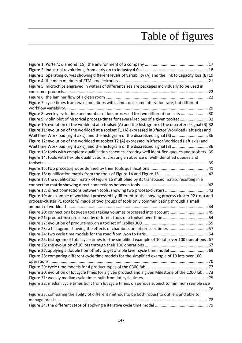
147
Table of figures
Figure 1: Porter’s diamond [15], the environment of a company ........................................................ 17 Figure 2: industrial revolutions, from early on to Industry 4.0 ............................................................. 18 Figure 3: operating curves showing different levels of variability (A) and the link to capacity loss (B) 19 Figure 4: the main markets of STMicroelectronics ............................................................................... 21 Figure 5: microchips engraved in wafers of different sizes are packages individually to be used in consumer products................................................................................................................................ 22 Figure 6: the laminar flow of a clean room ........................................................................................... 22 Figure 7: cycle times from two simulations with same tool, same utilization rate, but different workflow variability ............................................................................................................................... 29 Figure 8: weekly cycle time and number of lots processed for two different toolsets ........................ 30 Figure 9: violin plot of historical process-times for several recipes of a given toolset ......................... 31 Figure 10: evolution of the workload at a toolset (A) and the histogram of the discretized signal (B) 32 Figure 11: evolution of the workload at a toolset T1 (A) expressed in Xfactor Workload (left axis) and WaitTime Workload (right axis); and the histogram of the discretized signal (B) ................................ 36 Figure 12: evolution of the workload at toolset T2 (A) expressed in Xfactor Workload (left axis) and WaitTime Workload (right axis); and the histogram of the discretized signal (B) ................................ 36 Figure 13: tools with complete qualification schemes, creating well identified queues and toolsets . 39 Figure 14: tools with flexible qualifications, creating an absence of well-identified queues and toolsets .................................................................................................................................................. 39 Figure 15: two process-groups defined by their tools qualifications .................................................... 41 Figure 16: qualification matrix from the tools of Figure 14 and Figure 15 ........................................... 42 Figure 17: the qualification matrix of Figure 16 multiplied by its transposed matrix, resulting in a connection matrix showing direct connections between tools. ........................................................... 42 Figure 18: direct connections between tools, showing two process-clusters ...................................... 43 Figure 19: an example of workload processed by different tools, showing process-cluster P2 (top) and process-cluster P1 (bottom) made of two groups of tools only communicating through a small amount of workload .............................................................................................................................. 44 Figure 20: connections between tools taking volumes processed into account .................................. 45 Figure 21: product-mix processed by different tools of a toolset over time ........................................ 54 Figure 22: evolution of product-mix on a toolset of Crolles 300 .......................................................... 55 Figure 23: a histogram showing the effects of chambers on lot process-times ................................... 57 Figure 24: two cycle time models for the road from Lyon to Paris ....................................................... 64 Figure 25: histogram of total cycle times for the simplified example of 10 lots over 100 operations . 67 Figure 26: the evolution of 10 lots through their 100 operations ........................................................ 67 Figure 27: applying a double homothety to get a triple layer cycle time model .................................. 69 Figure 28: comparing different cycle time models for the simplified example of 10 lots over 100 operations ............................................................................................................................................. 70 Figure 29: cycle time models for 4 product types of the C300 fab ....................................................... 72 Figure 30: evolution of lot cycle times for a given product and a given Milestone of the C200 fab .... 73 Figure 31: weekly median cycle times built from lot cycle times ......................................................... 75 Figure 32: median cycle times built from lot cycle times, on periods subject to minimum sample size ............................................................................................................................................................... 76 Figure 33: comparing the ability of different methods to be both robust to outliers and able to manage breaks ...................................................................................................................................... 78 Figure 34: the different steps of applying a iterative cycle time model ............................................... 79
148
Figure 35: the concurrent WIP of a job p as the sum of the workloads of other jobs theoretically processed in job p Effective Waiting-Time window on the same process-cluster................................ 84 Figure 36 : concurrent WIP against observed capacities ...................................................................... 88 Figure 37: number of arrivals per week from real data (A) and generated by removing dependencies (B) .......................................................................................................................................................... 95 Figure 38: historical Down-Time/ Up-Time from a specific Crolles 300 tool over a year ..................... 96 Figure 39 : three possible outcomes when comparing 𝑪𝑻𝟎 to the sample population 𝑪𝑻𝒊, 𝒊 ≠ 𝟎 ..... 98 Figure 40 : uncertainty areas around 𝑪𝑻𝟎 and 𝑰𝟗𝟓 ............................................................................. 98 Figure 41 : operating curve showing 𝑪𝑻𝟎 statistically higher than μ (A), non-statistically different (B) and statistically lower than μ (C) ......................................................................................................... 103 Figure 42: evolution of workload waiting at a toolset of C300 fab. .................................................... 114 Figure 43: the effect of increased product-mix on process-clusters with setups or batches ............. 114 Figure 44: historical workload for a period of 1 month ...................................................................... 118 Figure 45 : workload profile from the raw simulation compared to the historical profile ................. 119 Figure 46 : workload profile from the fitted simulation compared to the historical profile .............. 121 Figure 47 : workload profile from a simulation with historical arrivals, but no downtime variability 124 Figure 48 : workload profile from a simulation with historical downtimes, but no arrivals variability ............................................................................................................................................................. 125 Figure 49 : workload profile from a simulation with no product-mix ................................................. 126 Figure 50 : workload profile from a simulation with no arrivals variability and no downtime variability ............................................................................................................................................................. 127 Figure 51 : the impact of PM segregation on workload accumulations (Kosta Rozen, MASM 2016). 133 Figure 52 : the impact of local PM segregation on fab cycle times (Kosta Rozen, MASM 2016) ........ 134

149
Table of tables
Table 1: sources of variability identified by authors related to the variability of semiconductor manufacturing. The sources of variability are ordered by the number of times identified in the literature. ............................................................................................................................................... 51 Table 2: operation cycle times for the simplified example of 10 lots over 100 operations.................. 66 Table 3 : results of the experiment framework tested on 19 tools down/up sequences from STMicroelectronics .............................................................................................................................. 102 Table 4 : results of the experiment framework tested on 6 toolsets arrivals sequences from STMicroelectronics .............................................................................................................................. 104 Table 5 : results of the experiment framework tested on 19 tools process-time sequences from STMicroelectronics .............................................................................................................................. 105


151
References
[1] G. Q. Zhang, F. Van Roosmalen, and M. Graef, “The paradigm of ‘More than Moore,’” in 6th
International Conference on Electronic Packaging Technology, 2005, pp. 17–24.
[2] K. Dequeant, P. Vialletelle, P. Lemaire, and M. Espinouse, “A literature review on variability
in semiconductor manufacturing: the next forward leap to Industry 4.0,” in Winter Simulation
Conference (WSC), 2016, pp. 2598–2609.
[3] K. Dequeant, P. Lemaire, M. Espinouse, and P. Vialletelle, “Le WIP Concurrent : une
proposition de file d’attente du point de vue du produit pour caracteriser le temps de cycle,” in
11th International Conference on Modeling, Optimization & SIMulation, 2016.
[4] J. Robinson, “Sources of variability in wafer fabs,” FabTime Cycle Time Management
Newsletter, vol. 18, no. 2, pp. 3–4, 2017.
[5] A. K. Erlang, “The theory of probabilities and telephone conversations,” Nyt Tidsskrift for
Matematik B, vol. 20, no. 6, pp. 87–98, 1909.
[6] D. G. Kendall, “Stochastic Processes Occurring in the Theory of Queues and their Analysis by
the Method of the Imbedded Markov Chain,” The Annals of Mathematical Statistics, vol. 24,
no. 3, pp. 338–354, 1953.
[7] F. Pollaczek, “Über eine aufgabe der wahrscheinlichkeitstheorie. I.,” Mathematische
Zeitschrift, vol. 32, no. 1, pp. 64–100, 1930.
[8] W. Whitt, “The queueing network analyzer,” The Bell System Technical Journal, vol. 62, no. 9,
pp. 2779–2815, 1983.
[9] J. Abate and W. Whitt, “Transient behavior of the M/M/l queue: Starting at the origin,”
Queueing Systems, vol. 2, no. 1, pp. 41–65, 1987.
[10] K. W. Fendick and W. Whitt, “Measurements and approximations to describe the offered
traffic and predict the average workload in a single-server queue,” in Proceedings of the IEEE,
1989, vol. 77, no. 1, pp. 171–194.
[11] W. Whitt, “Approximations for the GI/G/m queue,” Production and Operations Management,
vol. 2, no. 2, pp. 114–161, 1993.
[12] W. Hopp and M. Spearman, Factory physics: foundations of factory management. Chicago,
IL.: InvinIMcGraw Hill, 1996.
[13] J. D. C. Little, “A proof for the queuing formula: L=$lambda$W,” Operations Research, vol.
9, no. 3, pp. 383–387.
[14] R. Shah and P. T. Ward, “Lean manufacturing: Context, practice bundles, and performance,”
Journal of Operations Management, vol. 21, no. 2, pp. 129–149, 2003.
[15] M. E. Porter, “The competitive advantage of nations,” Harvard business review, vol. 68, no. 2,
pp. 73–93, 1990.
[16] M. Brettel, N. Friederichsen, M. Keller, and M. Rosenberg, “How virtualization,
decentralization and network building change the manufacturing landscape: an Industry 4.0
perspective,” International Journal of Mechanical, Aerospace, Industrial, Mechatronic and
Manufacturing Engineering, vol. 8, no. 1, pp. 37–44, 2014.
[17] S. S. Aurand and P. J. Miller, “The operating curve : a method to measure and benchmark
manufacturing line productivity,” in Advanced Semiconductor Manufacturing Conference,
1997, pp. 391–397.
[18] S. M. Brown, T. Hanschke, I. Meents, B. R. Wheeler, and H. Zisgen, “Queueing model
improves IBM’s semiconductor capacity and lead-time management,” Interfaces, vol. 40, no.
152
5, pp. 397–407, 2010.
[19] D. Delp, J. Si, and J. W. Fowler, “The development of the complete X-Factor contribution
measurement for improving cycle time and cycle time variability,” IEEE Transactions on
Semiconductor Manufacturing, vol. 19, no. 3, pp. 352–362, 2006.
[20] L. F. P. Etman, C. P. L. Veeger, E. Lefeber, I. J. B. F. Adan, and J. E. Rooda, “Aggregate
modeling of semiconductor equipment using effective process times,” in Winter Simulation
Conference (WSC), 2011, pp. 1790–1802.
[21] J. P. Ignizio, “Estimating the sustainable capacity of semiconductor fab workstations,”
International Journal of Production Research, vol. 49, no. 17, pp. 5121–5131, 2011.
[22] D. Kim, W. Lixin, and R. Havey, “Measuring cycle time through the use of the queuing theory
formula (G/G/M),” in Winter Simulation Conference (WSC), 2014, pp. 2216–2226.
[23] D. P. Martin, “Capacity and cycle time - throughput understanding system (CAC-TUS) an
analysis tool to determine the components of capacity and cycle time in a semiconductor
manufacturing Line,” in Advanced Semiconductor Manufacturing Conference (ASMC), 1999,
pp. 127–131.
[24] J. Robinson, J. Fowler, and E. Neacy, “Capacity loss factors in semiconductor manufacturing,”
2003.
[25] A. K. Schoemig, “On the corrupting influence of variability in Semiconductor Manufacturing,”
in Winter Simulation Conference (WSC), 1999, pp. 837–842.
[26] J. G. Shanthikumar, S. Ding, and M. T. Zhang, “Queueing theory for semiconductor
manufacturing systems : a survey and open problems,” Transactions on Automation Science
and Engineering, vol. 4, no. 4, pp. 513–522, 2007.
[27] I. Tirkel, “The effectiveness of variability reduction in decreasing wafer cycle time,” in Winter
Simulation Conference (WSC), 2013, pp. 3796–3805.
[28] K. Wu, “An examination of variability and its basic properties for a factory,” IEEE
Transactions on Semiconductor Manufacturing, vol. 18, no. 1, pp. 214–221, 2005.
[29] H. Zisgen and I. Meents, “A queueing network based system to model capacity and cycle time
for semiconductor fabrication,” in Winter Simulation Conference (WSC), 2008, pp. 2067–2074.
[30] D. Delp, J. Si, Y. Hwang, and B. Pei, “A dynamic system regulation measure for increasing
effective capacity: the X-factor theory,” in Advanced Semiconductor Manufacturing
Conference (ASMC), 2003, pp. 81–88.
[31] L. Mönch, J. W. Fowler, S. Dauzère-Pérès, S. J. Mason, and O. Rose, “A survey of problems,
solution techniques, and future challenges in scheduling semiconductor manufacturing
operations,” Journal of Scheduling, vol. 14, no. 6, pp. 583–599, 2011.
[32] T. Frazee and C. Standridge, “Conwip versus POLCA: A comparative analysis in a high-mix,
low-volume (HMLV) manufacturing environment with batch processing,” Journal of Industrial
Engineering and Management, vol. 9, no. 2, pp. 432–449, 2016.
[33] J. H. Jacobs, P. P. Van Bakel, L. F. P. Etman, and J. E. Rooda, “Quantifying variability of
batching equipment using effective process times,” IEEE Transactions on Semiconductor
Manufacturing, vol. 19, no. 2, pp. 269–275, 2006.
[34] R. Akhavan-tabatabaei, Y. Fathi, and J. G. Shanthikumar, “A markov chain framework for
cycle time approximation of toolsets,” IEEE Transactions on Semiconductor Manufacturing,
vol. 25, no. 4, pp. 589–597, 2012.
[35] R. E. A. Schelasin, “Estimating wafer processing cycle time using an improved G/G/m queue,”
in Winter Simulation Conference (WSC), 2013, pp. 3789–3795.
[36] K. Wu and K. Hui, “The determination and indetermination of service times in manufacturing
systems,” IEEE Transactions on Semiconductor Manufacturing, vol. 21, no. 1, pp. 72–81,
2008.
[37] J. H. Jacobs, L. F. P. Etman, E. J. J. Van Campen, and J. E. Rooda, “Characterization of
153
operational time variability using effective process times,” IEEE Transactions on
Semiconductor Manufacturing, vol. 16, no. 3, pp. 511–520, 2003.
[38] E. Mhiri, M. Jacomino, F. Mangione, P. Vialletelle, and G. Lepelletier, “Finite capacity
planning algorithm for semiconductor industry considering lots priority,” IFAC-PapersOnLine,
vol. 48, no. 3, pp. 1598–1603, 2015.
[39] A. Lima, V. Borodin, S. Dauzère-pérès, and P. Vialletelle, “A decision support system for
managing line stops of time constraint tunnels,” in 40th International Convention on
Information and Communication Technology, Electronics and Microelectronics (MIPRO),
2017, pp. 309–314.
[40] M. Rowshannahad, S. Dauzère-Pérès, and B. Cassini, “Qualification management to reduce
workload variability in semiconductor manufacturing,” in Winter Simulation Conference
(WSC), 2014, pp. 2434–2443.
[41] S. Gurumurthi and S. Benjaafar, “Modeling and analysis of flexible queueing systems,” Naval
Research Logistics, vol. 51, no. 5, pp. 755–782, 2004.
[42] Z. Chen and H. Ji, “Graph-based clustering for computational linguistics: A survey,” in
workshop on Graph-based Methods for Natural Language Processing, 2010, pp. 1–9.
[43] G. W. Flake, R. E. Tarjan, and K. Tsioutsiouliklis, “Graph clustering and minimum cut trees,”
Internet Mathematics, vol. 1, no. 4, pp. 385–408, 2004.
[44] H. Sakasegawa, “An approximation formula L q≃ α· ρ β/(1-ρ).,” Annals of the Institute of
Statistical Mathematics, vol. 29, no. 1, 1977.
[45] O. Rose, M. Dümmler, and A. Schömig, “On the validity of approximation formulae for
machine downtimes,” Inst. für Informatik. 2000.
[46] M. G. Huang, P. L. Chang, and Y. C. Chou, “Analytic approximations for multiserver batch-
service workstations with multiple process recipes in semiconductor wafer fabrication,” IEEE
Transactions on Semiconductor Manufacturing, vol. 14, no. 4, pp. 395–405, 2001.
[47] S. Karabuk and S. D. Wu, “Coordinating strategic capacity planning in the semiconductor
industry,” Operations Research, vol. 51, no. 6, pp. 839–849, 2003.
[48] J. R. Morrison and D. P. Martin, “Cycle time approximations for the G/G/m queue subject to
server failures and cycle time offsets with applications,” in Advanced Semiconductor
Manufacturing Conference (ASMC), 2006, pp. 322–326.
[49] T. Hanschke, “Approximations for the mean queue length of the GIX/G(b,b)/c queue,”
Operations Research Letters, vol. 34, pp. 205–213, 2006.
[50] J. R. Morrison and D. P. Martin, “Practical extensions to cycle time approximations for the
G/G/m-Queue with applications,” IEEE Transactions on Automation Science and Engineering,
vol. 4, no. 4, pp. 523–532, 2007.
[51] R. Hirade, R. Raymond, and H. Okano, “Sensitivity analysis on causal events of WIP bubbles
by a log-driven simulator,” in Winter Simulation Conference (WSC), 2007, pp. 1747–1754.
[52] W. J. Hopp, S. M. R. Iravani, and B. Shou, “A diagnostic tree for improving production line
performance,” Production and Operations Management, vol. 16, no. 1, pp. 77–92, 2007.
[53] S. Chang, S. Su, and K. Chen, “Priority-mix planning for cycle time-differentiated
semiconductor manufacturing services,” in Winter Simulation Conference (WSC), 2008, pp.
2251–2259.
[54] R. Akhavan-Tabatabaei, S. Ding, and J. G. Shanthikumar, “A method for cycle time estimation
of semiconductor manufacturing toolsets with correlations,” in Winter Simulation Conference
(WSC), 2009, pp. 1719–1729.
[55] J. P. Ignizio, “Cycle time reduction via machine-to-operation qualification,” International
Journal of Production Research, vol. 47, no. 24, pp. 6899–6906, 2009.
[56] R. Schelasin, “Using static capacity modeling and queuing theory equations to predict factory
cycle time performance in semiconductor manufacturing,” in Winter Simulation Conference

154
(WSC), 2011, pp. 2045–2054.
[57] R. C. Leachman, “The Engineering Management of Speed,” in Industry Studies Association
Annual Conference, 2012.
[58] A. a. Kalir, “Segregating preventive maintenance work for cycle time optimization,” IEEE
Transactions on Semiconductor Manufacturing, vol. 26, no. 1, pp. 125–131, 2013.
[59] M. G. Filho and R. Uzsoy, “The impact of simultaneous continuous improvement in setup time
and repair time on manufacturing cycle times under uncertain conditions,” International
Journal of Production Research, vol. 51, no. 2, pp. 1–18, 2012.
[60] A. Senderovich, M. Weidlich, A. Gal, and A. Mandelbaum, “Queue mining for delay
prediction in multi-class service processes,” Information Systems, vol. 53, pp. 278–295, 2015.
[61] K. Rozen and N. M. Byrne, “Using simulation to improve semiconductor factory cycle time by
segregation of preventive maintenance activities,” in Winter Simulation Conference (WSC),
2016, pp. 2676–2684.
[62] M. Hassoun, G. Rabinowitz, and S. Lachs, “Identification and cost estimation of WIP bubbles
in a fab,” IEEE Transactions on Semiconductor Manufacturing, vol. 21, no. 2, pp. 217–222,
2008.
[63] J. P. Ignizio, Optimizing factory performance. New York: McGraw-Hill.
[64] T. Pomorski, “Managing overall equipment effectiveness [OEE] to optimize factory
performance,” in IEEE International Symposium on Semiconductor Manufacturing, 1997, pp.
33–36.
[65] E. Padonou, O. Roustant, and M. Lutz, “Robust monitoring of an industrial IT system in the
presence of structural change,” Quality and Reliability Engineering International, vol. 31, no.
6, pp. 949–962, 2015.
[66] J. Ledolter and B. Abraham, “Some comments on the initialization of exponential smoothing,”
Journal of Forecasting, vol. 3, no. 1, pp. 79–84, 1984.
[67] C. Leys, C. Ley, O. Klein, P. Bernard, and L. Licata, “Detecting outliers: Do not use standard
deviation around the mean, use absolute deviation around the median,” Journal of
Experimental Social Psychology, vol. 49, no. 4, pp. 764–766, 2013.
[68] J. D. C. Little, “Little’s law as viewed on its 50th anniversary,” Operations Research, vol. 59,
no. 3, pp. 536–549, 2011.
[69] W. S. Cleveland and S. J. Devlin, “Locally weighted regression: An approach to regression
analysis by local fitting,” Journal of the American Statistical Association, vol. 83, no. 403, pp.
596–610, 1988.
[70] E. Mhiri, M. Jacomino, F. Mangione, P. Vialletelle, and G. Lepelletier, “A step toward capacity
planning at finite capacity in semiconductor manufacturing,” in Winter Simulation Conference
(WSC), 2015, pp. 2239–2250.
[71] E. Albey, Ü. Bilge, and R. Uzsoy, “An exploratory study of disaggregated clearing functions
for production systems with multiple products,” International Journal of Production Research,
vol. 52, no. 18, pp. 5301–5322, 2014.
[72] S. Ahn and J. a. Fessler, “Standard errors of mean, variance, and standard deviation
estimators,” EECS Department, University of Michigan. pp. 1–2, 2003.
[73] I. Sutskever, O. Vinyals, and Q. V. Le, “Sequence to sequence learning with neural networks,”
in Advances in Neural Information Processing Systems (NIPS), 2014, pp. 3104–3112.
[74] T.-H. Wen, M. Gasic, N. Mrksic, P.-H. Su, D. Vandyke, and S. Young, “Semantically
conditioned LSTM-based natural language generation for spoken dialogue systems,” in
Conference on Empirical Methods in Natural Language Processing, 2015, pp. 1711–1721.

156
Summary
In the context of Industry 4.0 and the More than Moore’s paradigm, delivery precision and short
cycle times are essential to the competitiveness of High Mix Low Volume semiconductor manufacturing
and future industries in general. So called “variability” however creates uncontrolled and unpredictable
“traffic-jams” in manufacturing systems, increasing cycle times and decreasing the systems’ tractability.
This research, a CIFRE PhD between the GSCOP laboratory and STMicroelectronics, addresses this
issue of variability in complex manufacturing environment. We first conducted, in the first part of the
manuscript, an in-depth study of “variability”: we approached the notion through its consequences in
manufacturing systems, clarified that the variability was about the workflow, introducing the notion of
workflow variability and measures that come with it, and identified the main sources of variability
through a literature review and real-world examples. We focused in the second part of this manuscript
on the integration of workflow variability in production management tools: we showed how integrating
the stable consequences of workflow variability can improve WIP projections in complex systems and
increase the control on such systems, proposed a new tool (the concurrent WIP) to better measure the
performances of systems subject to high workflow variability, and showed that complex “dependency”
mechanisms play a key role in workflow variability yet are not integrated in any model. Finally, the
third and last part of the manuscript organized perspectives for variability reduction: based on the work
of this manuscript, we showed a framework for variability reduction on the short term, and proposed a
direction for medium and long term research.
Dans un contexte où l’industrie du semi-conducteur explore de nouvelles voies avec la
diversification des produits et le paradigme de « More than Moore », les délais de livraison et la
précision de livraison sont des éléments clés pour la compétitivité d’entreprises de semi-conducteur et
l’industrie 4.0 en général. Les systèmes de production sont cependant sujets à de la « variabilité », qui
crée des embouteillages dans la production de manière incontrôlée et imprévisible. Cette thèse CIFRE
(partenariat entre le laboratoire GSCOP et STMicroelectronics) s’attaque à ce problème de la variabilité
dans la fabrication en environnement complexe. La première partie de cette thèse offre une étude
approfondie de la variabilité : nous mettons d’abord en avant les conséquences de la variabilité pour
mieux la définir, puis nous clarifions que la variabilité concerne les flux de production en introduisant
la notion de variabilité des flux de production et en apportant des éléments de mesure associés, et nous
clôturons cette première partie par l’étude des sources de variabilité à travers une étude bibliographique
et des exemples industriels. La seconde partie est dédiée à l’intégration de la variabilité dans les outils
de gestion de production: nous montrons comment une partie des conséquences peut être mesurée et
intégrée aux projections d’encours pour améliorer le contrôle et la prévisibilité de la production,
proposons un nouvel outil (le WIP concurrent) pour mesurer plus précisément les performances des
systèmes en environnement complexe, et mettons en avant des effets de dépendances prépondérants sur
la variabilité des flux de production et pourtant jamais pris en compte dans les modèles. La troisième et
dernière partie de la thèse couvre les perspectives de réduction de la variabilité : en se basant sur les
éléments présentés dans la thèse, nous proposons un plan pour réduire la variabilité des flux de
production sur le court terme, et une direction pour la recherche à moyen et long terme.