Embed Size (px)
Citation preview

W P 1 1 - 1 0 A P r i l 2 0 1 1
Working Paper S e r i e s
1750 Massachusetts Avenue, NW Washington, DC 20036-1903 Tel: (202) 328-9000 Fax: (202) 659-3225 www.piie.com
The Liquidation of Government DebtCarmen M. Reinhart and M. Belen Sbrancia
Abstract
Historically, periods of high indebtedness have been associated with a rising incidence of default or restructuring of public and private debts. A subtle type of debt restructuring takes the form of “financial repression.” Financial repression includes directed lending to government by captive domestic audiences (such as pension funds), explicit or implicit caps on interest rates, regulation of cross-border capital movements, and (generally) a tighter connection between government and banks. In the heavily regulated financial markets of the Bretton Woods system, several restrictions facilitated a sharp and rapid reduction in public debt/GDP ratios from the late 1940s to the 1970s. Low nominal interest rates help reduce debt servicing costs while a high incidence of negative real interest rates liquidates or erodes the real value of government debt. Thus, financial repression is most successful in liquidating debts when accompanied by a steady dose of inflation. Inflation need not take market participants entirely by surprise and, in effect, it need not be very high (by historical standards). For the advanced economies in our sample, real interest rates were negative roughly half of the time during 1945–80. For the United States and the United Kingdom our estimates of the annual liquidation of debt via negative real interest rates amounted on average to 3 to 4 percent of GDP a year. For Australia and Italy, which recorded higher inflation rates, the liquidation effect was larger (around 5 percent per annum). We describe some of the regulatory measures and policy actions that characterized the heyday of the financial repression era.
JEL Codes: E2, E3, E6, F3, F4, H6, N10Keywords: Public Debt, Financial Repression, Inflation, Interest Rates, Debt Liquidation, Default,
Restructuring, Debt Reduction
Carmen M. Reinhart is the Dennis Weatherstone Senior Fellow at the Peterson Institute for International Economics. She was previously professor of economics and director of the Center for International Economics at the University of Maryland. She was earlier chief economist and vice president at the investment bank Bear Stearns in the 1980s and spent several years at the International Monetary Fund. She is a research associate at the National Bureau of Economic Research, research fellow at the Centre for Economic Policy Research, and member of the Congressional Budget Office Panel of Economic Advisers and Council on Foreign Relations. She is the recipient of the 2010 TIAA-CREF Paul A. Samuelson Award. Her best-selling book entitled This Time is Different: Eight Centuries of Financial Folly, which has been translated into 13 languages, documents the striking similarities of the recurring booms and busts that have characterized financial history. M. Belen Sbrancia is a research assistant and PhD candidate at the University of Maryland.
Note: The authors wish to thank Alex Pollock, Vincent Reinhart, Kenneth Rogoff, Ross Levine and Luc Laeven for helpful comments and suggestions. We also thank the participants of the April 2011 IMF conference on “Macro-Financial Stability in the New Normal,” and the National Science Foundation Grant No. 0849224 for financial support.
Copyright © 2011 by the Peterson Institute for International Economics. All rights reserved. No part of this working paper may be reproduced or utilized in any form or by any means, electronic or mechanical, including
photocopying, recording, or by information storage or retrieval system, without permission from the Institute.

2
I. IntroductIon
Some people will think the 2¾ nonmarketable bond is a trick issue. We want to meet that head on. It is. It is an attempt to lock up as much as possible of these longer-term issues.
—Assistant Secretary of the Treasury William McChesney Martin, Jr.1
The decade that preceded the outbreak of the subprime crisis in the summer of 2007 produced a record
surge in private debt in many advanced economies, including the United States. The period prior to
the 2001 burst of the “tech bubble” was associated with a marked rise in the leverage of nonfinancial
corporate business; in the years 2001–07, debts of the financial industry and households reached unprec-
edented heights.2 The decade following the crisis may yet mark a record surge in public debt during
peacetime, at least for the advanced economies. It is not surprising that debt reduction, of one form or
another, is a topic that is receiving substantial attention in academic and policy circles alike.3
Throughout history, debt/GDP ratios have been reduced by (1) economic growth; (2) substantive
fiscal adjustment/austerity plans; (3) explicit default or restructuring of private and/or public debt; (4) a
sudden surprise burst in inflation; and (5) a steady dosage of financial repression that is accompanied by
an equally steady dosage of inflation. (Financial repression is defined in box 1.) It is critical to clarify that
options (4) and (5) are viable only for domestic-currency debts. Since these debt reduction channels are
not necessarily mutually exclusive, historical episodes of debt reduction have owed to a combination of
more than one of these channels.4
Hoping that substantial public and private debt overhangs are resolved by growth may be uplifting,
but it is not particularly practical from a policy standpoint. The evidence, at any rate, is not particularly
encouraging, as high levels of public debt appear to be associated with lower growth.5 The effectiveness of
1. FOMC minutes, March 1–2, 1951, remarks on the 1951 conversion of short-term marketable US Treasury debts for 29-year nonmarketable bonds. Martin subsequently became chairman of the Board of Governors, 1951–70.
2. The surge in private debt is manifest in both the gross external debt figures of the private sector (see Lane and Milesi-Ferretti 2010, for careful and extensive historical documentation since 1970 and Reinhart, http://terpconnect.umd.edu/~creinhar, for a splicing of their data with the latest IMF/World Bank figures) and domestic bank credit (as documented in Reinhart 2010). Relative to GDP, these debt measures reached unprecented heights during 2007–10 in many advanced economies.
3. Among recent studies, see Alesina and Ardagna (2009), IMF (2010), Lilico, Holmes, and Sameen (2009) on debt reduction via fiscal adjustment and Sturzenegger and Zettlemeyer (2006), Reinhart and Rogoff (2009) and sources cited therein on debt reduction through default and restructuring.
4. For instance, in analyzing external debt reduction episodes in emerging markets, Reinhart, Rogoff, and Savastano (2003) suggest that default and debt restructuring played a leading role in most of the episodes they identify. However, in numerous cases the debt restructurings (often under the umbrella of IMF programs) were accompanied by debt repayments associated with some degree of fiscal adjustment.
5. See Checherita and Rother (2010), Kumar and Woo (2010), and Reinhart and Rogoff (2010).

3
fiscal adjustment/austerity in reducing public debt—and particularly, their growth consequences (which
are the subject of some considerable debate)—is beyond the scope of this paper. Reinhart and Rogoff
(2009, 2011a) analyze the incidence of explicit default or debt restructuring (or forcible debt conversions)
among advanced economies (through and including World War II episodes) and emerging markets as well
as hyperinflation as debt reduction mechanisms.
The aim of this paper is to document the more subtle and gradual form of debt restructuring or
“taxation” that has ocurred via financial repression (as defined in box 1). We show that such repression
helped reduce lofty mountains of public debt in many of the advanced economies in the decades
following World War II and subsequently in emerging markets, where financial liberalization is of more
recent vintage.6 We find that financial repression in combination with inflation played an important role
in reducing debts. Inflation need not take market participants entirely by surprise and, in effect, it need
not be very high (by historic standards). In effect, financial repression via controlled interest rates, directed
credit, and persistent, positive inflation rates is still an effective way of reducing domestic government
debts in the world’s second largest economy, China.7
Prior to the 2007 crisis, it was deemed unlikely that advanced economies could experience financial
meltdowns of a severity to match those of the pre–World War II era; the prospect of a sovereign default
in wealthy economies was similarly unthinkable.8 Repeating that pattern, the ongoing discussion of how
public debts have been reduced in the past has focused on the role played by fiscal adjustment. It thus
appears that it has also been collectively “forgotten” that the widespread system of financial repression
that prevailed for several decades (1945–1980s) worldwide played an instrumental role in reducing or
“liquidating” the massive stocks of debt accumulated during World War II in many of the advanced
countries, United States inclusive.9 We document this phenomenon.
6. In a recent paper, Aizenman and Marion (2010) stress the important role played by inflation in reducing US World War II debts and develop a framework to highlight how the government may be tempted to follow that route in the near future. However, the critical role played by financial repression (regulation) in keeping nominal interest rates low and producing negative real interest rates was not part of their analysis.
7. Bai et al. (2001), for example, present a framework that provides a general rationale for financial repression as an implicit taxation of savings. They argue that when effective income tax rates are very uneven, as common in developing countries, raising some government revenue through mild financial repression can be more efficient than collecting income tax only.
8. The literature and public discussion surrounding “the great moderation” attests to this benign view of the state of the macroeconomy in the advanced economies. See, for example, McConnell and Perez-Quiros (2000).
9. For the political economy of this point see the analysis presented in Alesina, Grilli, and Milesi-Ferretti (1993). They present a framework and stylized evidence to support that strong governments coupled with weak central banks may impose capital controls so as to enable them to raise more seigniorage and keep interest rates artificially low—facilitating domestic debt reduction.

4
The next section discusses how previous “debt overhang” episodes have been resolved since 1900.
There is a brief sketch of the numerous defaults, restructurings, conversions (forcible and “voluntary”) that
dealt with the debts of World War I and the Great Depression. This narrative, which follows Reinhart and
Rogoff (2009, 2011a), primarily serves to highlight the substantially different route taken after World War
II to deal with the legacy of high war debts.
Section III provides a short description of the types of financial-sector policies that facilitated the
liquidation of public debt. Hence, our analysis focuses importantly on regulations affecting interest rates
Box 1 Financial repression defined
The term financial repression was introduced in the literature by the works of Edward Shaw (1973) and Ronald McKinnon (1973). Subsequently, the term became a way of describing emerging-market financial systems prior to the widespread financial liberalization that began in the 1980 (see Agenor and Montiel 2008 for an excellent discus-sion of the role of inflation and Giovannini and de Melo 1993 and Easterly 1989 for country-specific estimates). However, as we document in this paper, financial repression was also the norm for advanced economies during the post–World War II period and in varying degrees up through the 1980s. We describe here some of its main features.
Pillars of financial repression
1. Explicit or indirect caps or ceilings on interest rates, particularly (but not exclusively) those on government debts. These interest rate ceilings could be effected through various means, including (1) explicit government regulation (for instance, Regulation Q in the United States prohibited banks from paying interest on demand deposits and capped interest rates on saving deposits); (2) ceilings on banks’ lending rates, which were a direct subsidy to the government in cases where it borrowed directly from the banks (via loans rather than securitized debt); and (3) interest rate cap in the context of fixed coupon rate nonmarketable debt or (4) maintained through central bank interest rate targets (often at the directive of the Treasury or Ministry of Finance when central bank independence was limited or nonexistent). Allan Meltzer’s (2003) monumental history of the Federal Reserve (volume I) documents the US experience in this regard; Alex Cukierman’s (1992) classic on central bank indepen-dence provides a broader international context.
2. creation and maintenance of a captive domestic audience that facilitated directed credit to the government. This was achieved through multiple layers of regulations from very blunt to more subtle measures. (1) Capital account restrictions and exchange controls orchestrated a “forced home bias” in the portfolio of financial insti-tutions and individuals under the Bretton Woods arrangements. (2) High reserve requirements (usually nonre-munerated) as a tax levy on banks (see Brock 1989 for an insightful international comparison). Among more subtle measures, (3) “prudential” regulatory measures requiring that institutions (almost exclusively domestic ones) hold government debts in their portfolios (pension funds have historically been a primary target). (4) Transaction taxes on equities (see Campbell and Froot 1994) also act to direct investors toward government (and other) types of debt instruments. And (5) prohibitions on gold transactions.
3. other common measures associated with financial repression aside from the ones discussed above are (1) direct ownership (e.g., in China or India) of banks or extensive management of banks and other financial institu-tions (e.g., in Japan) and (2) restricting entry into the financial industry and directing credit to certain industries (see Beim and Calomiris 2000).

5
(with the explicit intent on keeping these low) and on policies creating “captive” domestic audiences that
would hold public debts (in part achieved through capital controls, directed lending, and an enhanced
role for nomarketable public debts).
We also focus on the evolution of real interest rates during the era of financial repression (1945–
1980s). We show that real interest rates were significantly lower during 1945–80 than in the freer capital
markets before World War II and after financial liberalization. This is the case irrespective of the interest
rate used—whether central bank discount, treasury bills, deposit, or lending rates and whether for
advanced or emergingmarkets. For the advanced economies, real ex post interest rates were negative in
about half of the years of the financial repression era compared with less than 15 percent of the time since
the early 1980s.
In section IV, we provide a basic conceptual framework for calculating the “financial repression
tax,” or more specifically, the annual “liquidation rate” of government debt. Alternative measures are
also discussed. These exercises use a detailed database on a country’s public debt profile (coupon rates,
maturities, composition, etc.) from 1945 to 1980 constructed by Sbrancia (2011). This “synthetic” public
debt portfolio reflects the actual shares of debts across the different spectra of maturities as well as the
shares of marketable versus nonmarketable debt (the latter involving both securitized debt as well as direct
bank loans).
Section V presents the central findings of the paper, which are estimates of the annual “liquidation
tax” as well as the incidence of liquidation years for ten countries (Argentina, Australia, Belgium, India,
Ireland, Italy, South Africa, Sweden, the United Kingdom, and the United States). For the United States
and the United Kingdom, the annual liquidation of debt via negative real interest rates amounted to 3 to
4 percent of GDP on average per year. Such annual deficit reduction quickly accumulates (even without
any compounding) to a 30 to 40 percent of GDP debt reduction in the course of a decade. For other
countries that recorded higher inflation rates, the liquidation effect was even larger. As to the incidence of
liquidation years, Argentina sets the record with negative real rates recorded every single year from 1945
to 1980.
Section VI examines the question of whether inflation rates were systematically higher during
periods of debt reduction in the context of a broader 28-country sample that spans both the heyday
of financial repression and the periods before and after. We describe the algorithm used to identify the
largest debt reduction episodes on a country-by-country basis and show that in 21 of the 28 countries
inflation was higher during the larger debt reduction periods.
Finally, we discuss some of the implications of our analysis for the current debt overhang and
highlight areas for further research. Two appendices to this paper (1) compare our methodology to other
approaches in the literature that have been used to measure the extent of financial repression or calculate

6
the financial repression tax; (2) provide country-specific details on the behavior of real interest rates across
regimes; and (3) describe the coverage and extensive sources for the data compiled for this study.
II. deFAult, restructurIng And conversIons: HIgHlIgHts From tHe 1920s to tHe 1950s
Peaks and troughs in public debt/GDP are seldom synchronized across many countries’ historical
paths. There are, however, a few historical episodes where global (or nearly global) developments, be
it a war or a severe financial and economic crisis, produce a synchronized surge in public debt, such
as the one recorded for advanced economies since 2008. Using the Reinhart and Rogoff (2011a)
database for 70 countries, figure 1 provides central government debt/GDP for the advanced and
emerging economies subgroups since 1900. It is a simple arithmetic average that does not assign weight
according to country size.
global debt surges and their resolution
An examination of these two series identifies a total of five peaks in world indebtedness. Three episodes
(World War I, World War II, and the Second Great Contraction, 2008–present) are almost exclusively
advanced-economy debt peaks; one is unique to emerging markets (1980s debt crisis followed by the
transition economies’ collapses); and the Great Depression of the 1930s is common to both groups.
World War I and Depression debts were importantly resolved by widespread default and explicit restruc-
turings or predominantly forcible conversions of domestic and external debts in both the now-advanced
economies and the emerging markets. Notorious hyperinflation in Germany, Hungary, and other parts
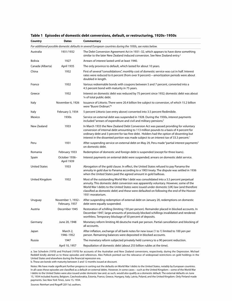
of Europe violently liquidated domestic-currency debts. Table 1 and the associated discussion provide
a chronology of these debt resolution episodes. As Reinhart and Rogoff (2009, 2011a) document, debt
reduction via default or restructuring has historically been associated with substantial declines in output
in the run-up to as well as during the credit event and in its immediate aftermath.
The World War II debt overhang was importantly liquidated via the combination of financial
repression and inflation, as we shall document. This was possible because debts were predominantly
domestic and denominated in domestic currencies. The robust postwar growth also contributed
importantly to debt reduction in a way that was a marked contrast to the 1930s, when the combined
effects of deflation and output collapses worked to worsen the debt/GDP balance in the way stressed by
Irving Fisher (1933).
The resolution of the emerging-market debt crisis involved a combination of default or restructuring
of external debts, explicit default, or financial repression on domestic debt. In several episodes, notably in
Latin America, hyperinflation in the mid-to-late 1980s and early 1990s completed the job of significantly

7
liquidating (at least for a brief interlude) the remaining stock of domestic currency debt (even when such
debts were indexed, as was the case of Brazil). 10
default, restructurings, and Forcible conversions in the 1930s
Table 1 lists the known “domestic credit events” of the Depression. Default on or restructuring of external
debt (see the extensive notes to the table) also often accompanied the restructuring or default of the
domestic debt. All the Allied governments, with the exception of Finland, defaulted on (and remained in
default through 1939 and never repaid) their World War I debts to the United States as economic condi-
tions deteriorated worldwide during the 1930s.11
Thus, the high debts of World War I and the subsequent debts associated with the Depression of the
1930s were resolved primarily through default and restructuring. Neither economic growth nor inflation
contributed much. In effect, for all 21 now-advanced economies, the median annual inflation rate for
1930–39 was barely above zero (0.4 percent).12 Real interest rates remained high through significant
stretches of the decade.
It is important to stress that during the period after World War I the gold standard was still in place
in many countries, which meant that monetary policy was subordinated to keep a given gold parity. In
those cases, inflation was not a policy variable available to policymakers in the same way that it was after
the adoption of fiat currencies.
III. FInAncIAl rePressIon: PolIcIes And evIdence From reAl Interest rAtesselected Financial regulation measures during the “era of Financial repression”
One salient characteristic of financial repression is its pervasive lack of transparency. The reams of regula-
tions applying to domestic and cross-border financial transactions and directives cannot be summarized
by a brief description. Table 2 makes this clear by providing a broad sense of the kinds of regulations
on interest rates and cross-border and foreign exchange transactions and how long these lasted since the
end of World War II in 1945. A common element across countries’ “financial architecture” not brought
out in table 2 is that domestic government debt played a dominant role in domestic institutions’ asset
holdings—notably that of pension funds. High reserve requirements, relative to the current practice
in advanced economies and many emerging markets, were also a common way of taxing the banks not
captured in our minimalist description. The interested reader is referred to Brock (1989) and Agenor
10. Backward-looking indexation schemes are not particularly effective in hyperinflationary conditions.
11. Finland, being under threat of Soviet invasion at the time, maintained payments on its debts to the United States so as to maintain the best possible relationship.
12. See Reinhart and Rogoff (2010).

8
and Montiel (2008), who focus on the role of reserve requirements and their link to inflation (see also
appendix table A.2 and accompanying discussion.)
real Interest rates
One of the main goals of financial repression is to keep nominal interest rates lower than would otherwise
prevail. This effect, other things equal, reduces the governments’ interest expenses for a given stock of debt
and contributes to deficit reduction. However, when financial repression produces negative real interest
rates, this also reduces or liquidates existing debts. It is a transfer from creditors (savers) to borrowers (in
the historical episode under study here—the government).
The financial repression tax has some interesting political-economy properties. Unlike income,
consumption, or sales taxes, the “repression” tax rate (or rates) are determined by financial regulations
and inflation performance that are opaque to the highly politicized realm of fiscal measures. Given that
deficit reduction usually involves highly unpopular expenditure reductions and (or) tax increases of one
form or another, the relatively “stealthier” financial repression tax may be a more politically palatable
alternative to authorities faced with the need to reduce outstanding debts. As discussed in Obstfeld and
Taylor (2004) and others, liberal capital-market regulations (the accompanying market-determined
interest rates) and international capital mobility reached their heyday prior to World War I under the
umbrella of the gold standard. World War I and the suspension of convertibility and international gold
shipments it brought, and, more generally, a variety of restrictions on cross-border transactions were the
first blows to the globalization of capital. Global capital markets recovered partially during the roaring
twenties, but the Great Depression, followed by World War II, put the final nails in the coffin of laissez
faire banking. It was in this environment that the Bretton Woods arrangement of fixed exchange rates and
tightly controlled domestic and international capital markets was conceived.13 In that context, and taking
into account the major economic dislocations, scarcities, etc. which prevailed at the closure of the second
great war, we witness a combination of very low nominal interest rates and inflationary spurts of varying
degrees across the advanced economies. The obvious result were real interest rates—whether on treasury
bills (figure 2), central bank discount rates (figure 3), deposits (figure 4), or loans (not shown)—that were
markedly negative during 1945–46.
For the next 35 years or so, real interest rates in both advanced and emerging economies would
remain consistently lower than the eras of freer capital mobility before and after the financial repression
13. In a framework where there are both tax collection costs and a large stock of domestic government, Aizenman and Guidotti (1994) show how a government can resort to capital controls (which lower domestic interest rates relative to foreign interest rates) to reduce the costs of servicing the domestic debt.

9
era. In effect, real interest rates (figures 2 to 4) were on average negative.14 Binding interest rate ceilings
on deposits (which kept real ex post deposit rates even more negative than real ex post rates on treasury
bills, as shown in figures 2 and 4) “induced” domestic savers to hold government bonds. What delayed
the emergence of leakages in the search for higher yields (apart from prevailing capital controls) was that
the incidence of negative returns on government bonds and on deposits was (more or less) a universal
phenomenon at this time.15 The frequency distributions of real rates for the period of financial repression
(1945–80) and the years following financial liberalization (roughly 1981–2009 for the advanced
economies) shown in the three panels of figure 5 highlight the universality of lower real interest rates prior
to the 1980s and the high incidence of negative real interest rates.
Such negative (or low) real interest rates were consistently and substantially below the real rate of
growth of GDP; this is consistent with the observation of Elmendorf and Mankiw (1999) when they state
“An important factor behind the dramatic drop (in US public debt) between 1945 and 1975 is that the
growth rate of GNP exceeded the interest rate on government debt for most of that period.” They fail to
explain why this configuration should persist over three decades in so many countries.
Real interest rates on deposits were negative in about 60 percent of the observations. In effect, real
ex post deposit rates were below one percent about 83 percent of the time. Appendix table A.1, which
shows for each country average real interest rates during the financial repression period (the dates vary, as
highlighted in table 2, depending on when interest rates were liberalized) and thereafter, substantiates our
claims that low and negative real interest rates (by historical standards) were the norm across countries
with very different levels of economic development.
The preceding analysis sets the general tone of what to expect, in terms of real rates of return on a
portfolio of government debt, during the era of financial repression. For the United States, for example,
Homer and Sylla (2005) describe 1946–81 as the second (and longest) bear bond market in US history.16
To reiterate the point that the low real interest rates of the financial repression era were exceptionally low
in relation to not only the post-liberalization period but also the more liberal financial environment of
pre-World War II, figure 6 plots the frequency distribution of real interest rates on deposits for the United
Kingdom over three subperiods, 1880–1939,17 1945–80, and 1981–2010.
14. Note that real interest rates were lower in a high economic growth period of 1945–80 than in the lower growth period 1981–2009; this is exactly the opposite of the prediction of a basic growth model and therefore indicative of significant impediments to financial trade.
15. A comparison of the return on government bonds to that of equity during this period and its connection to “the equity premium puzzle” can be found in Sbrancia (2011).
16. They identify 1899–1920 as the first US bear bond market.
17. Excluding the World War I period.

10
The preceding analysis of real interest rates despite being qualitatively suggestive falls short of
providing estimates of the magnitude of the debt-servicing savings and outright debt liquidation that
accrued to governments during this extended period. To fill in that gap the next section outlines the
methodological approach we follow to quantify the financial repression tax, while section V presents the
main results.
Iv. lIquIdAtIon oF government deBt: concePtuAl And dAtA Issues
This section discusses the data and methodology we develop to arrive at estimates of how much debt was
liquidated via a combination of low nominal interest rates and higher inflation rates, or what we term “the
liquidation effect.”18
Data Requirements. Reliable estimates of the liquidation effect require considerable data, most of
which are not readily available from even the most comprehensive electronic databases. Indeed, most of
the data used in these exercises come from a broad variety of historical government publications, many
which are quite obscure, as detailed in data appendix B. The calculation of the “liquidation effect” is a
clear illustration of a case where the devil lies in the details, as the structure of government debt varies
enormously across countries and within countries over time. Differences in coupon rates, maturity,
distribution of marketable and nonmarketable debt, and securitized debt versus loans from financial
institutions importantly shape the overall cost of debt financing for the government. There is no “single”
government interest rate (such as a 3-month t-bill or a 10-year bond) that is appropriate to apply to
a hybrid debt stock. The starting point to come up with a measure that reflects the true cost of debt
financing is a reconstruction of the government’s debt profile over time.
Sample. We employ two samples in our empirical analysis. We use the database from Sbrancia (2011) of
the government’s debt profiles for 10 countries (Argentina, Australia, Belgium, India, Ireland, Italy, South
Africa, Sweden, the United Kingdom, and the United States). These were constructed from primary
sources over the period 1945–90 where possible or over shorter intervals (determined by data availability)
for a subset of the sample. For the benchmark or basic calculations (described below), this involves
data on a detailed composition of debt, including maturity, coupon rate, and outstanding amounts
by instrument. For a more comprehensive measure, which takes into account capital gains or losses of
holding government debt, bond price data are also required. In all cases, we also use official estimates of
consumer price inflation, which at various points in history may significantly understate the true inflation
18. Appendix table A.2 and its accompanying discussion also examines other approaches to quantifying the financial repression tax.
11
rates.19 Data on nominal GDP and government tax revenues are used to express the estimates of the
liquidation effect as ratios that are comparable across time and countries.
For our broader analysis of the behavior of inflation during major debt reduction episodes, which
has far less demanding data requirements (domestic public debt outstanding/GDP and inflation rates),
our sample broadens to 28 countries from all regions for 1790–2010 (or subsamples therein). The
countries and their respective coverage are listed in appendix table A.3.
Benchmark Basic estimates of the “liquidation effect”
Debt Portfolio. We construct a “synthetic portfolio”20 for the government’s total debt stock at the
beginning of the year (fiscal or calendar, as noted). This portfolio reflects the actual shares of debts across
the different spectra of maturities as well as the shares of marketable versus nonmarketable debt.
Interest Rate on the Portfolio. The “aggregate” nominal interest rate for a particular year is the coupon
rate on a particular type of debt instrument weighted by that instrument’s share in the total stock of debt. 21 We then aggregate across all debt instruments. The real rate of interest,
t
ttt
ir
11 (1)
(where i and π are nominal interest and inflation rates, respectively) is calculated on an ex post basis using
consumer price index (CPI) inflation for the corresponding one-year period. It is a before-tax real rate of
return (excluding capital gains or losses).22
19. This is primarily due to the existence of price controls, which were mainly imposed during World War II and remained for several years after the end of the conflict. See Friedman and Schwartz (1982) for estimates of the actual price level in the United States and United Kingdom and Wiles (1952) for post–World War II United Kingdom.
20. The term “synthetic” is used in the sense that a hypothetical investor holds the total portfolio of government debt at the beginning of the period, which is defined as either the beginning of the calendar year or the fiscal year, depending on how the debt data are reported by the particular country. Country specifics are detailed in data appendix B. The weights in this hypothetical portfolio are given by the actual shares of each component of debt in the total domestic debt of the government.
21. Giovannini and de Melo (1993) state “the choice of a ‘representative’ interest rate on domestic liabilities an almost impossible task and because there are no reliable breakdowns of domestic and foreign liabilities by type of loan and interest rate charged.” This is precisely the almost impossible task we undertake here. Their alternative methodology is described in appendix table A.2.
22. Some of the observations on inflation are sufficiently high to make the more familiar linear version of the Fisher equation a poor approximation.

12
Definition of Debt “Liquidation Years.” Our benchmark calculations define a liquidation year as one in
which the real rate of interest (as defined above) is negative (below zero). This is a conservative definition
of liquidation year; a more comprehensive definition would include periods where the real interest rate on
government debt was below a “market” real rate.23
Savings to the Government During Liquidation Years. This concept captures the savings (in interest
costs) to the government from having a negative real interest rate on government debt. (As noted it is
a lower bound on saving of interest costs, if the benchmark used assumed, for example, a positive real
rate of, say, 2 or 3 percent.) These savings can be thought of as having “a revenue equivalent” for the
government, which like regular budgetary revenues can be expressed as a share of GDP or as a share of
recorded tax revenues to provide standard measures of the “liquidation effect” across countries and over
time. The saving (or “revenue”) to the government or the “liquidation effect” or the “financial repression
tax” is the real (negative) interest rate times the “tax base,” which is the stock of domestic government
debt outstanding.
Alternative measure of the liquidation effect Based on total returns
Thus far, our measure of the liquidation affect has been confined to savings to the government by way
of annual interest costs. However, capital losses (if bond prices fall) may also contribute importantly
to the calculus of debt liquidation over time. This is the case because the market value of the debt will
actually be lower than its face value. The market value of government debt obviously matters for investors’
wealth but also measures the true capitalized value of future coupon and interest payments. Moreover, a
government (or its central bank) buying back existing debt could directly and immediately lower the par
value of existing obligations. Once we take into account potential price changes, the total nominal return
or holding period return (HPR) for each instrument is given by:
1
1 )(
t
tttt P
CPPHPR (2)
where Pt and Pt–1 are the prices of the bond at time t and t–1, respectively, and Ct is the annual interest
payment (i.e., the nominal coupon rate).
We use this total return measure as a supplement rather than as our core or benchmark “liquidation
measure” (despite the fact that it incorporates more information on the performance of the bond
portfolio). Bond price data are available only for a subset of the securities that constitute the government
23. However, determining what such a market rate would be in periods of pervasive financial repression requires assumptions about whether real interest rates during that period would have comparable to the real interest that prevailed in the period when markets were liberalized and prices were market determined.

13
portfolio and, more generally, consistent time series price data are more difficult to get for some of the
countries in our sample. It is also worth noting that while price movements for different bonds are
generally in the same direction during a particular year, there are significant differences in the magnitudes
of the price changes. This cross-bond variation in price performance makes it difficult to infer the price of
nonmarketable debt (for which there are no price data altogether), as well as marketable bonds for which
there are no price data. As before, we define “liquidation years” as those periods in which the real return
of the portfolio is negative.
role of Inflation and currency depreciation
The idea of governments using inflation to liquidate debt is hardly a new one since the widespread
adoption of fiat currency, as discussed earlier.24 It is obvious that for any given nominal interest rate a
higher inflation rate reduces the real interest rate on the debt, thus increasing the odds that real interest
rates become negative and the year is classified as a “liquidation year.” Furthermore, it is also evident that
for any year that is classified as a liquidation year the higher the inflation rate (for a given coupon rate) the
higher the saving to the government.
Our approach helps to pinpoint periods (and countries) when inflation played a systematically
larger role in eroding the debts of the government. In addition, we can disentangle to what extent this
was done via relatively short-lived “inflation surprises” (unanticipated inflation) or through a steady and
chronic dose of moderate inflation over extended time horizons. Because we do not have a direct measure
of inflation expectations for much of the sample, we define inflation bursts or “surprises” in a more
mechanical, ex post manner. Specifically, we calculate a ten-year moving average for inflation and classify
those years in which inflation was more than two standard deviations above the 10-year average as an
“inflation burst/surprise year.” As the 10-year window may be arbitrarily too backward looking, we also
perform the comparable exercise using a five-year moving average.
v. lIquIdAtIon oF government deBt: emPIrIcAl estImAtes
This section presents estimates of the “liquidation effect” for ten advanced and emerging economies
for most of the post–World War II period. Our main interest lies in the period prior to the process of
financial liberalization that took hold during the 1980s—that is, the era of financial repression. However,
as noted, this three-plus decade-long stretch is by no means uniform. The decade immediately following
World War II was characterized by a very high public debt overhang—legacy of the war, a higher
incidence of inflation, and often multiple currency practices (with huge black market exchange rate
24. See, for example, Calvo’s (1989) framework, which highlights the role of inflation in debt liquidation even in the presence of short-term debt.

14
premiums) in many advanced economies.25 The next decade (1960s) was the heyday of the Bretton Woods
system with heavily regulated domestic and foreign exchange markets and more stable inflation rates in
the advanced economies (as well as more moderate public debt levels). The 1970s was quite distinct from
the prior decades, as leakages in financial regulations proliferated, the fixed exchange rate arrangements
under Bretton Woods among the advanced economies broke down, and inflation began to resurface in the
wake of the global oil shock and accommodative monetary policies in the United States and elsewhere. To
this end, we also provide estimates of the liquidation of government debt for relevant subperiods.
Incidence and magnitude of the “liquidation tax”
Table 3 provides information on a country-by-country basis for the period under study; the incidence of
debt liquidation years (as defined in the preceding section); the listing of the liquidation years; the average
(negative) real interest rate during the liquidation years; and the minimum real interest rate recorded (and
the year in which that minimum was reached). Given its notorious high and chronic inflation history
coupled with heavy-handed domestic financial regulation and capital controls during 1944–74, it is not
surprising that Argentina tops the list. Almost all the years (97 percent) were recorded as liquidation years,
as the Argentine real ex post interest rates were negative in every single year during 1944–74 except for
1953 (a just deflationary year). For India, that share was 53 percent (slightly more than one half of the
1949–80 observations recorded negative real interest rates). Before reaching the conclusion that this debt
liquidation through financial repression was predominantly an emerging-market phenomenon, it is worth
noting that for the United Kingdom the share of liquidation years was about 48 percent during 1945–80.
For the United States, the world’s financial center, a quarter of the years during that same period Treasury
debt had negative real interest rates.
As to the magnitudes of the financial repression tax (table 3), real interest rates were most negative
for Argentina (reaching a minimum of –53 percent in 1959). The share of domestic government debt
in Argentina (and other Latin American countries) in total (domestic plus external) public debt was
substantial during 1900–1950s; it is not surprising that in light of these real rates the domestic debt
market all but disappeared and capital flight marched upwards (capital controls notwithstanding). By the
late 1970s Argentina and many other chronic inflation countries were predominantly relying on external
debt.26 Italian real interest rates right after World War II were as negative as 47 percent (in 1945). For the
Unites States real rates were –8 to –9 percent during 1945–47 (on average the United States had –3.5
percent real rates during the liquidation years).
25. See De Vries (1969), Horsefield (1969), Reinhart and Rogoff (2002).
26. See Reinhart and Rogoff’s (2011) forgotten history of domestic debt.

15
There are two distinct patterns in the ten-country sample evident from an inspection of the timing
of the incidence and magnitude of the negative real rates. The first of these is the cases where the negative
real rates (financial repression tax) were most pronounced in the years following World War II (as war
debts were importantly inflated away). This pattern is most evident in Australia, the United Kingdom,
and the United States, although negative real rates reemerge following the breakdown of Bretton Woods
in 1974–75. Then there are the cases where there is a more persistent or chronic reliance on financial
repression throughout the sample as a way of funding government deficits and/or eroding existing
government debts. The cases of Argentina and India in the emerging markets and Ireland and Italy in the
advanced economies stand out in this regard.
The preceding analysis, as noted, adopts a very narrow, conservative calculation of both the incidence
of the “liquidation effect” or the financial repression tax. Much of the literature on growth, as well as
standard calibration exercises involving subjective rates of time preference assume benchmark real interest
rates of 3 percent per annum and even higher. Thus, a threshold that only examines periods where real
interest rates were actually negative is bound to underestimate the incidence of “abnormally low” real
interest rates during the era of financial repression (approximately taken to be 1945–80). To assess the
incidence of more broadly defined low real interest rates, table 4 presents for the 10 core countries the
share of years where real returns on a portfolio of government debt (as defined earlier) were below zero (as
in table 3), 1, 2, and 3 percent, respectively.27
In the era of financial repression that we examine here, real ex post interest rates on government debt
did not reach 3 percent in a single year in the United States; in effect in nearly two-thirds of the years real
interest rates were below 1 percent. The incidence of “abnormally low” real interest rates is comparable for
the United Kingdom and Australia—both countries had sharp and relatively rapid declines in public debt
to GDP following World War II.28 Even in countries with substantial economic and financial volatility
during this period (including Ireland, and Italy), real interest rates on government debt above 3 percent
were relatively rare (accounting for only about 20 to 23 percent of the observations).
estimates of the liquidation effect
Having documented the high incidence of “liquidation years” (even by conservative estimates), we now
calculate the magnitude of the savings to the government (financial repression tax or liquidation effect).
These estimates take “the tax rate” (the negative real interest rate) and multiply it by the “tax base” or the
stock of debt. Table 5 reports these estimates for each country.
27. An alternative strategy would be to use a growth model to calibrate the relationship between the real interest rate and output growth for the counterfactual of free markets. That, however, would make the results model specific.
28. “Abnormally low” by the historical standards that include periods of liberalized financial markets before and after 1945–80; see Homer and Sylla’s (2005) classic book for a comprehensive and insightful history of interest rates.
16
The magnitudes are in all cases nontrivial, irrespective of whether we use the benchmark measure
that is exclusively based on interest rate (coupon yields) or the alternative measure that includes capital
gains (or losses) for the cases where the bond price data are available.
For the United States and the United Kingdom the annual liquidation of debt via negative real
interest rates amounted on average to 3 and 4 percent of GDP a year. Obviously, annual deficit reduction
of 3 to 4 percent of GDP quickly accumulates (even without any compounding) to a 30 to 40 percent of
GDP debt reduction in the course of a decade. For Australia and Italy, which recorded higher inflation
rates, the liquidation effect was larger (around 5 percent per annum). Interestingly (but not entirely
surprising), the average annual magnitude of the liquidation effect for Argentina is about the same as that
of the United States, despite the fact that the average real interest rate averaged about –3.5 percent for the
United States and nearly –16 percent for Argentina during liquidation years in the 1945–80 repression
era. Just as money holdings secularly shrink during periods of high and chronic inflation, so does the
domestic debt market.29 Argentina’s “tax base” (domestic public debt) shrank steadily during this period;
at the end of World War II nearly all public debt was domestic and by the early 1980s domestic debt
accounted for less than half of total public debt. Without the means to liquidate external debts, Argentina
defaulted on its external obligations in 1982.
Countries like Ireland, India, Sweden, and South Africa that did not experience a massive public
debt build-up during World War II recorded more modest annual savings (but still substantive) during
the heyday of financial repression.30
vI. InFlAtIon And deBt reductIon
We have argued that inflation is most effective in liquidating government debts (or debts in general),
when interest rates are not able to respond to the rise in inflation and in inflation expectations.31 This
disconnect between nominal interest rates and inflation can occur if (1) the setting is one where interest
rates are either administered or predetermined (via financial repression, as described); (2) all government
debts are fixed-rate and long maturities and the government has no new financing needs (even if there is
no financial repression, the long maturities avoid rising interest costs that would otherwise prevail if short
maturity debts needed to be rolled over); and (3) all (or nearly all) debt is liquidated in one “surprise”
inflation spike.
29. These issues are examined in Reinhart and Rogoff (2011).
30. It is important to note that while financial repression wound down in most of the advanced economies in the sample by the mid-1980s, it has persisted in varying degrees in India through the present (with its system of state-owned banks and widespread capital controls) and in Argentina (except for the years of the “Convertibility Plan,” April 1991–December 2001).
31. That is, the coefficient in the Fisher equation is less than one.

17
Our attention thus far has been confined to the first on that list: the financial repression
environment. The second scenario, where governments only have long-term, fixed-rate debt outstanding
and have no new financing needs, (deficits) remain to be identified (however, we have a sense such
episodes are relatively rare). This leaves the third case where debts are swiftly liquidated via an inflation
spike (or perhaps more appropriately surge). To attempt to identify potential episodes of the latter, we
conduct two simple exercises.
In the first exercise, we identify inflation “surprises” for the core ten-country sample. In order
to identify inflation surprises we calculate a 10-year moving average inflation, and count a year as
an “inflation surprise” year if the inflation during that year is two standard deviations above the
corresponding 10-year average.32 Table 7 presents the results. The second column shows the share of years
which are “inflation surprises” during the sample period while the third shows the share of years which are
both an “inflation surprise” and a “liquidation year.”
As table 7 highlights, there is not much overlap between debt liquidation years and inflation
surprises, as defined here. Averaging across the 10 countries, only 18 percent of the liquidation years
coincide with an “inflation surprise.” The high incidence of inflation surprise years during the early 1970s
at the time of the surge in oil and commodity prices suggests our crude methodology to identify “inflation
surprises (or spikes)” may be a reasonable approximation to the real thing. More to the point, this exercise
suggests that the role of inflation in the liquidation of debt is predominantly of the more chronic variety
coupled with financially repressed nominal interest rates.
Our algorithm for the second exercise begins by identifying debt reduction episodes and then
focusing on the largest of these. Any decline in debt/GDP over a three-year window classifies as
a debt-reduction episode. For this pool of debt reduction episodes, we construct their frequency
distribution (for each country) and focus on the lower (10 percent) tail of the distribution to identify
the “largest” three-year debt reduction episodes. This algorithm biases our selection of episodes toward
the more sudden (or abrupt) ones (even if these are later reversed), which might a priori be attributable
to some combination of a booming economy, a substantive fiscal austerity plan, a burst in inflation/
liquidation, or explicit default or restructuring. A milder but steady debt reduction process that lasts
over many years would be identified as a series of episodes—but if the decline in debt over any particular
three-year window is modest it may not be large enough to fall in the lower 10 percent of all the
observations.
This exercise helps flag episodes where inflation is likely to have played a significant role in public
debt reduction but does not provide estimates of how much debt was liquidated (as in the preceding
32. The pertinent 10-year average for determining whether year t is an inflation surprise or not is calculated over the interval t–10 to t–1.

18
analysis). Because we only require information on domestic public debt/GDP and inflation, we expand
our coverage to 28 countries predominantly (but not exclusively) over 1900–2009. Thus, we are not
exclusively focusing on the period of financial repression but examining more broadly the role of inflation
and debt reduction in the countries’ histories.
Table 8 lists the largest debt reduction episodes by country. The last year of the three-year
episode is shown for each country; the year that appears in italics represents the largest single-episode
of debt reduction. The next two columns of the table are devoted to the average and median inflation
performance during the debt reduction episodes listed in the second column in comparison to the
inflation performance (average and median) for the full sample (the coverage, which varies by country,
is shown in appendix table A.3). In 22 of 28 countries, inflation is significantly higher in the episodes
of debt reduction than for the full sample. In the extreme cases, it is the wholesale liquidation of
domestic debt, such as during the German hyperinflation of the early 1920s and the long-lasting
Brazilian and Argentine hyperinflations of the early 1990s. Even without these extreme cases, the
inflation differentials between the debt reduction episodes and the full sample are suggestive of the use of
inflation (intentionally or because it became unmanageable) to reduce (or liquidate) government debts
even in periods outside the era of heavy financial repressions. The evidence is only suggestive of this
interpretation, as no explicit causal pattern is tested.
vII. concludIng remArks
The substantial tax on financial savings imposed by the financial repression that characterized 1945–80
was a major factor explaining the relatively rapid reduction of public debt in a number of the advanced
economies. This fact has been largely overlooked in the literature and discussion on debt reduction. The
United Kingdom’s history offers a pertinent illustration. Following the Napoleonic Wars, the United
Kingdom’s public debt was a staggering 260 percent of GDP; it took over 40 years to bring it down to
about 100 percent (a massive reduction in an era of price stability and high capital mobility anchored by
the gold standard). Following World War II, the United Kingdom’s public debt ratio was reduced by a
comparable amount in 20 years.33
The financial repression route taken at the creation of the Bretton Woods system was facilitated by
initial conditions after the war, which had left a legacy of pervasive domestic and financial restrictions.
Indeed, even before the outbreak of World War II, the pendulum had begun to swing away from laissez-
33. Peak debt/GDP was 260.6 percent in 1819 and 237.9 percent in 1947. Real GDP growth was about the same during the two debt reduction periods (1819–59) and (1947–67), averaging about 2.5 percent per annum (the comparison is not exact as continuous GDP data begin in 1830). As such, higher growth cannot obviously account for the by far faster debt reduction following World War II.

19
faire financial markets toward heavier-handed regulation in response to the widespread financial crises of
1929–31. But one cannot help thinking that part of the design principle of the Bretton Woods system
was to make it easier to work down massive debt burdens. The legacy of financial crisis made it easier to
package those policies as prudential.
To deal with the current debt overhang, similar policies to those documented here may reemerge in
the guise of prudential regulation rather than under the politically incorrect label of financial repression.
Moreover, the process where debts are being “placed” at below-market interest rates in pension funds and
other more captive domestic financial institutions is already under way in several countries in Europe.
There are many bankrupt (or nearly so) pension plans at the state level in the United States that bear
scrutiny (in addition to the substantive unfunded liabilities at the federal level).
Markets for government bonds are increasingly populated by nonmarket players, notably central
banks of the United States, Europe, and many of the largest emerging markets, calling into question what
the information content of bond prices are relatively to their underlying risk profile. This decoupling
between interest rates and risk is a common feature of financially repressed systems. With public and
private external debts at record highs, many advanced economies are increasingly looking inward for
public debt placements.
While to state that initial conditions on the extent of global integration are vastly different at the
outset of Bretton Woods in 1946 and today is an understatement, the direction of regulatory changes
have many common features. The incentives to reduce the debt overhang are more compelling today than
about half a century ago. After World War II, the overhang was limited to public debt (as the private
sector had painfully deleveraged through the 1930s and the war); at present, the debt overhang many
advanced economies face encompasses (in varying degrees) households, firms, financial institutions, and
governments.
reFerences
Agénor, Pierre-Richard, and Peter J. Montiel, 2008. Development Macroeconomics, 3d ed. Princeton: Princeton University Press.
Aizenman, Joshua, and Pablo Guidotti. 1994. Capital Controls, Collection Costs, and Domestic Public Debt. Journal of International Money and Finance (February): 41–54.
Aizenman, Joshua, and Nancy Marion. 2010. Using Inflation to Erode the U.S. Public Debt. SCIIE Working Paper 09-13 (December). Santa Cruz Institute for International Economics, Department of Economics at the University of California, Santa Cruz.
Alesina, Alberto, Vittorio Grilli, and Gian Maria Milesi-Ferretti. 1993. The Political Economy of Capital Controls. In Capital Mobility: New Perspectives, ed. L. Leiderman and A. Razin. Cambridge, UK: Cambridge University Press.

20
Alesina, Alberto, and Silvia Ardagna. 2009. Large Changes in Fiscal Policy: Taxes versus Spending. NBER Working Paper 15438. Cambridge, MA: National Bureau of Economic Research.
Andima (Associação Nacional das Instituições do Mercado Financeiro). 1994. Divida Publica [Public Debt]. Rio de Janeiro, Brazil.
Bai, Chong-En, David D. Li, Yingyi Qian, and Yijang Wang. 2001. Financial Repression and Optimal Taxation. Economic Letters 70, no. 2 (February): 245–51.
Beim, David O., and Charles W. Calomiris. 2001. Emerging Financial Markets. New York: McGraw-Hill/Irwin.
Brock, Philip. 1989. Reserve Requirements and the Inflation Tax. Journal of Money, Credit and Banking 21, no. 1 (February): 106–121.
Calvo, Guillermo A. 1989. Is Inflation Effective in Liquidating Short-Term Nominal Debt? IMF Working Paper WP/89/2. Washington: International Monetary Fund.
Campbell, John Y., and Kenneth A. Froot. 1994. International Experiences with Securities Transactions Taxes. In The Internationalization of Equity Markets, ed. Jeffrey Frankel. Chicago: University of Chicago Press for NBER.
Checherita, Christina, and Philipp Rother. 2010. The Impact of High and Growing Debt on Economic Growth and Empirical Investigation for the Euro Area. ECB Working Paper 1237 (August). Frankfurt: European Central Bank.
Confalonieri, Antonio, and Emilio Gatti. 1986. La Politica del Debito Pubblico en Italia 1919–1943. Bari: Cariplo-Laterza.
Cukierman, Alex. 1992. Central Bank Strategy, Credibility, and Independence. Cambridge, MA: MIT Press.
DeVries, Margaret. 1969. The International Monetary Fund, 1945-1965: Twenty Years of International Monetary Cooperation. Volume II. Washington: International Monetary Fund.
Easterly, William R. 1989. Fiscal Adjustment and Deficit Financing During the Debt Crisis. In Dealing with the Debt Crisis, ed. I. Husain and I. Diwan. Washington: World Bank.
Easterly, William, and Klaus Schmidt-Hebbel. 1994. Fiscal Adjustment and Macroeconomic Performance. In Public Sector Deficits and Macroeconomic Performance, ed. W. Easterly et al. Oxford University Press for the World Bank.
Elmendorf, Douglas, and Gregory Mankiw. 1999. Government Debt. Handbook of Macroeconomics, volume 1, ed. J. B. Taylor and M. Woodford Elsevier Science, B.V.
Fisher, Irving. 1933. The Debt-Deflation Theory of Great Depressions. Econometrica 1, no. 4 (October): 337–57.
Fregert, Klas, and Roger Gustafsson. 2008. Fiscal Statistics for Sweden 1719–2003. Research in Economic History 25: 169–224.
Friedman, Milton, and Anna Schwartz. 1982. Monetary Trends in the United States and United Kingdom: Their Relation to Income, Prices, and Interest Rates, 1867-1975. Chicago: University of Chicago Press.
Giovannini, Alberto, and Martha de Melo. 1993. Government Revenue from Financial Repression. American Economic Review 83, no. 4: 953–63.
Homer, Sydney, and Richard Sylla. 2005. A History of Interest Rates, 4th ed. Hoboken, NJ: John Wiley & Sons, Inc.
Horsefield, J. Keith. 1969. The International Monetary Fund, 1945-1965: Twenty Years of International Monetary Cooperation. Volume I. Washington: International Monetary Fund.

21
IBGE (Instituto Brasileiro de Geografia e Estatística). 1990. Estatísticas históricas do Brasil: séries econômicas, demográficas e sociais de 1550 a 1988. Available at www.ibge.gov.br.
IMF (International Monetary Fund). 2010. World Economic Outlook. Washington.
Kumar, Manmohan S., and Jaejoon Woo. 2010. Public Debt and Growth. IMF Working Paper 10/174. Washington: International Monetary Fund.
Lane, Philip R., and Gian Maria Milesi-Ferretti. 2010. The External Wealth of Nations Mark II: Revised Extended Estimates of Foreign Assets and Liabilities, 1970–2004. In Macrofinancial Linkages: Trends, Crises, and Policies, ed. Crowe et al. Washington: International Monetary Fund.
Lilico, Andrew, Ed Holmes, and Hiba Sameen. 2009. Controlling Spending and Government Deficits: Lessons from History and International Experience. Controlling Public Spending Series. London: Policy Exchange.
McConnell, Margaret, and Gabriel Perez-Quiros. 2000. Output Fluctuations in the United States: What has Changed Since the Early 1980s? American Economic Review 90, no. 5: 1464–76.
McKinnon, Ronald I. 1973. Money and Capital in Economic Development. Washington: Brookings Institution.
Meltzer, Allan. 2003. A History of the Federal Reserve, Volume 1: 1913–1951. Chicago: Chicago University Press.
Montiel, Peter J. 2003. Macroeconomics in Emerging Markets, Cambridge: Cambridge University Press.
National Mining Association. 2006. The History of Gold. Mimeograph. Available at http://www.nma.org/pdf/gold/gold_history.pdf.
Obstfeld, Maurice, and Alan M. Taylor. 2004. Global Capital Markets: Integration, Crisis, and Growth. Japan-US Center Sanwa Monographs on International Financial Markets. Cambridge: Cambridge University Press.
Prichard, Muriel F. Lloyds. 1970. An Economic History of New Zealand to 1939. Auckland: Collins.
Reinhart, Carmen M. 2010. This Time is Different Chartbook: Country Histories on Debt, Default, and Financial Crises. NBER Working Paper 15815 (February). Cambridge, MA: National Bureau of Economic Research.
Reinhart, Carmen M., and Vincent R. Reinhart. 1999. On the Use of Reserve Requirements in Dealing with the Capital-Flow Problem. International Journal of Finance and Economics 4, no. 1 (January): 27–54.
Reinhart, Carmen M. and Kenneth Rogoff. 2002. The Modern History of Exchange Rate Arrangements: A Reinterpretation. NBER Working Paper 8963 (May). Cambridge, MA: National Bureau of Economic Research.
Reinhart, Carmen M., and Kenneth Rogoff. 2009. This Time is Different: Eight Centuries of Financial Folly. Princeton: Princeton University Press.
Reinhart, Carmen M. and Kenneth Rogoff. 2010. Growth in a Time of Debt. American Economic Review 100, no. 2 (May): 573–78.
Reinhart, Carmen M., and Kenneth Rogoff. 2011a. The Forgotten History of Domestic Debt. Forthcoming in the Economic Journal. Also published as NBER Working Paper 13946. Cambridge, MA: National Bureau of Economic Research.
Reinhart, Carmen M., and Kenneth Rogoff. 2011b. A Decade of Debt. NBER Working Paper 16827. Cambridge, MA: National Bureau of Economic Research.
Reinhart, Carmen M., Kenneth Rogoff, and Miguel A. Savastano. 2003. Debt Intolerance. Brooking Papers on Economic Activity 2003, no. 1: 1–62.

22
Sbrancia, M. Belen. 2011. Debt, Inflation, and the Liquidation Effect. University of Maryland, College Park. Mimeograph.
Schedvin, C. B. 1970. Australia and the Great Depression. Sydney: Sydney University Press.
Shaw, Edward S. 1973. Financial Deepening in Economic Development. New York: Oxford University Press.
Sturzenegger, Federico and Jeromin Zettelmeyer. 2006. Debt Defaults and Lessons from a Decade of Crises. Cambridge: MIT Press
Wiles, P. J. D. 1952. Pre-War and War-Time Controls In The British Economy, 1945–50. London: Oxford University Press.
23
table 1 episodes of domestic debt conversions, default, or restructuring, 1920s–1950scountry dates commentary
For additional possible domestic defaults in several European countries during the 1930s, see notes below.
Australia 1931/1932 The Debt Conversion Agreement Act in 1931–32, which appears to have done something similar to the later New Zealand induced conversion. See New Zealand entry.a
Bolivia 1927 Arrears of interest lasted until at least 1940.
Canada (Alberta) April 1935 The only province to default, which lasted for about 10 years.
China 1932 First of several “consolidations”, monthly cost of domestic service was cut in half. Interest rates were reduced to 6 percent (from over 9 percent)—amortization periods were about doubled in length.
France 1932 Various redeemable bonds with coupons between 5 and 7 percent, converted into a 4.5 percent bond with maturity in 75 years.
Greece 1932 Interest on domestic debt was reduced by 75 percent since 1932; domestic debt was about ¼ of total public debt.
Italy November 6, 1926 Issuance of Littorio. There were 20.4 billion lire subject to conversion, of which 15.2 billion were “Buoni Ordinari.”b
Italy February 3, 1934 5 percent Littorio (see entry above) converted into 3.5 percent Redimibile.
Mexico 1930s Service on external debt was suspended in 1928. During the 1930s, interest payments included “arrears of expenditure and civil and military pensions.”
New Zealand 1933 In March 1933 the New Zealand Debt Conversion Act was passed providing for voluntary conversion of internal debt amounting to 113 million pounds to a basis of 4 percent for ordinary debt and 3 percent for tax-free debt. Holders had the option of dissenting but interest in the dissented portion was made subject to an interest tax of 33.3 percent.1
Peru 1931 After suspending service on external debt on May 29, Peru made “partial interest payments” on domestic debt.
Romania February 1933 Redemption of domestic and foreign debt is suspended (except for three loans).
Spain October 1936– April 1939
Interest payments on external debt were suspended; arrears on domestic debt service.
United States 1933 Abrogation of the gold clause. In effect, the United States refused to pay Panama the annuity in gold due to Panama according to a 1903 treaty. The dispute was settled in 1936 when the United States paid the agreed amount in gold balboas.
United Kingdom 1932 Most of the outstanding World War I debt was consolidated into a 3.5 percent perpetual annuity. This domestic debt conversion was apparently voluntary. However, some of the World War I debts to the United States were issued under domestic (UK) law (and therefore classified as domestic debt) and these were defaulted on following the end of the Hoover 1931 moratorium.
Uruguay November 1, 1932–February, 1937
After suspending redemption of external debt on January 20, redemptions on domestic debt were equally suspended.
Austria December 1945 Restoration of schilling (limiting 150 per person). Remainder placed in blocked accounts. In December 1947, large amounts of previously blocked schillings invalidated and rendered worthless. Temporary blockage of 50 percent of deposits.
Germany June 20, 1948 Monetary reform limiting 40 deutsche mark per person. Partial cancellation and blocking of all accounts.
Japan March 2, 1946–1952
After inflation, exchange of all bank notes for new issue (1 to 1) limited to 100 yen per person. Remaining balances were deposited in blocked accounts.
Russia 1947 The monetary reform subjected privately held currency to a 90 percent reduction.
April 10, 1957 Repudiation of domestic debt (about 253 billion rubles at the time).
a. See Schedvin (1970) and Prichard (1970) for accounts of the Australian and New Zealand conversions, respectively, during the Depression. Michael Reddell kindly alerted us to these episodes and references. Alex Pollock pointed out the relevance of widespread restrictions on gold holdings in the United States and elsewhere during the financial repression era.b. These are bonds with maturity between 3 and 12 months issued at discount.
Notes: We have made significant further progress in sorting out the defaults on World War I debts to the United States, notably by European countries. In all cases these episodes are classified as a default on external debts. However, in some cases—such as the United Kingdom—some of the World War I debts to the United States were also issued under domestic law and, as such, would also qualify as a domestic default. The external defaults on June 15, 1934 included Austria, Belgium, Czechoslovakia, Estonia, France, Greece, Hungary, Italy, Latvia, Poland, and the United Kingdom. Only Finland made payments. See New York Times, June 15, 1934.
Sources: Reinhart and Rogoff (2011a); authors.

24
table 2 selected measures associated with financial repression
country
domestic financial regulation (liberalization year(s) in italics with emphasis on
deregulation of interest rates)
capital account exchange restrictions
(liberalization year(s)in italics)
Argentina 1977–82, 1987, and 1991–2001. Initial liberalization in 1977 was reversed in 1982. Alfonsin government undertook steps to deregulate the financial sector in October 1987, some interest rates being freed at that time. The Convertibility Plan, March 1991–2001, subsequently reversed.
1977–82 and 1991–2001. Between 1976 and 1978 multiple rate system was unified, foreign loans were permitted at market exchange rates, and all forex transactions were permitted up to US$ 20,000 by September 1978. Controls on inflows and outflows loosened over 1977–82. Liberalization measures were reversed in 1982. Capital and exchange controls eliminated in 1991 and reinstated on December 2001.
Australia 198. Deposit rate controls lifted in 1980. Most loan rate ceilings abolished in 1985. A deposit subsidy program for savings banks started in 1986 and ended in 1987.
1983. Capital and exchange controls tightened in the late 1970s, after the move to indirect monetary policy increased capital inflows. Capital account liberalized in 1983.
Brazil 1976–79 and 1989 onward. Interest rate ceilings removed in 1976, but reimposed in 1979. Deposit rates fully liberalized in 1989. Some loan rates freed in 1988. Priority sectors continue to borrow at subsidized rates. Separate regulation on interest rate ceilings exists for the microfi-nance sector
1984. System of comprehensive foreign exchange controls abolished in 1984. In the 1980’s most controls restricted outflows. In the 1990’s controls on inflows were strength-ened and those on outflows loosened and (once again) in 2010.
Canada 1967. With the revision of the Bank Act in 1967, interest rates ceilings were abolished. Further liberalizing measures were adopted in 1980 (allowing foreign banks entry into the Canadian market) and 1986.
1970. Mostly liberal regime.
Chile 1974 but deepens after 1984. Commercial bank rates liber-alized in 1974. Some controls reimposed in 1982. Deposit rates fully market determined since 1985. Most loan rates are market determined since 1984.
1979. Capital controls gradually eased since 1979. Foreign portfolio and direct investment is subject to a one year minimum holding period. During the 1990s, foreign borrowing is subject to a 30 percent reserve requirement.
Colombia 1980. Most deposit rates at commercial banks are market determined since 1980; all after 1990. Loan rates at commercial banks are market determined since the mid-1970s. Remaining controls lifted by 1994 in all but a few sectors. Some usury ceilings remain.
1991. Capital transactions liberalized in 1991. Exchange controls were also reduced. Large capital inflows in the early 1990s led to the reimposition of reserve require-ments on foreign loans in 1993.
Egypt 1991. Interest rates liberalized. Heavy “moral suasion” on banks remains.
1991. Decontrol and unification of the foreign exchange system. Portfolio and direct investment controls partially lifted in the 1990s.
Finland 1982. Gradual liberalization 1982–91. Average lending rate permitted to fluctuate within limits around the Bank of Finland base rate or the average deposit rate in 1986. Later in the year regulations on lending rates abolished. In 1987, credit guidelines discontinued, the Bank of Finland began open market operations in bank CDs and HELIBOR market rates were introduced. In 1988, floating rates allowed on all loans.
1982. Gradual liberalization 1982–91. Foreign banks allowed to establish subsidiaries in 1982. In 1984, domestic banks allowed to lend abroad and invest in foreign securities. In 1987, restrictions on long-term foreign borrowing on corporations lifted. In 1989, remaining regulations on foreign currency loans were abolished, except for households. Short-term capital movements liberalized in 1991. In the same year, house-holds were allowed to raise foreign currency denomi-nated loans.
France 1984. Interest rates (except on subsidized loans) freed in 1984. Subsidized loans now available to all banks, are subject to uniform interest ceiling.
1986. In the wake of the dollar crisis controls on in/outflows tightened. The extensive control system established by 1974, remains in place to early 80’s. Some restrictions lifted in 1983–85. Inflows were largely liberal-ized over 1986–88. Liberalization completed in 1990.
Germany 1980. Interest rates freely market determined from the 1970s to today. In the year indicated, further liberaliza-tions were undertaken.
1974. Mostly liberal regime in the late 60’s, Germany experiments with controls between 1970 and 1973. Starting 1974, controls gradually lifted, and largely elimi-nated by 1981.
(continued on next page)

25
table 2 selected measures associated with financial repression (continued)India 1992. Complex system of regulated interest rates simpli-
fied in 1992. Interest rate controls on Ds and commercial paper eliminated in 1993 and the gold market is liberal-ized. The minimum lending rate on credit over Rs 200,000 eliminated in 1994. Interest rates on term deposits of over two years liberalized in 1995.
1991. Regulations on portfolio and direct investment flows eased in 1991. The exchange rate was unified in 1993–94. Outflows remained restricted, and controls remained on private off-shore borrowing.
Italy 1983. Maximum rates on deposits and minimum rates on loans set by Italian Bankers’ Association until 1974. Floor prices on government bonds eliminated in 1992.
1985. Continuous operation of exchange controls in the 70’s. Fragile BoP delays opening in early 1980s. Starting in 1985, restrictions are gradually lifted. All remaining foreign exchange and capital controls eliminated by May 1990.
Japan 1979. Interest rate deregulation started in 1979. Gradual decontrol of rates as money markets grow and deepen after 1985. Interest rates on most fixed-term deposits eliminates by 1993. Non time deposits rates freed in 1994. Lending rates market determined in the 1990s (though they started in 1979, both external and domestic liberal-izations were very gradual and cautious).
1979. Controls on inflows eased after 1979. Controls on outflows eased in the mid-1980s. Forex restrictions eased in 1980. Remaining restrictions on cross border transac-tions removed in 1995.
Korea 1991. Liberalizing measures adopted in the early 1980s aimed at privatization and greater managerial leeway to commercial banks. Significant interest rate liberaliza-tion in four phases. Significant interest rate liberaliza-tion in four phases in the 90’s: 1991, 1993–94 and 1997. Most interest rate deregulated by 1995, except demand deposits and government supported lending.
1991. Current account gradually liberalized between 1985–87, and article VIII accepted in 1988. Capital account gradually liberalized, starting in 1991, usually following domestic liberalization. Restrictions on FDI and portfolio investment loosened in the early 1990s. Beginning with outflows, inflows to security markets allowed cautiously only in the mid 90’s. Complete liberalization planned for 2000.
Malaysia 1978–85 and 1987 onwards. Initially liberalized in 1978. Controls were reimposed in the mid-1980s (especially 1985–87) and abandoned in 1991.
1987. Measures for freer in/outflows of funds taken in 1973. Further ease of controls in 1987. Some capital controls reimposed in 1994. Liberalization of the capital account was more modest, and followed that of the current account.
Mexico 1977, deepens after 1988.Time deposits with flexible interest rates below a ceiling permitted in 1977. Deposit rates liberalized in 1988–89. Loan rates have been liberal-ized since 1988–89 except at development banks.
1985. Historically exchange regime much less restric-tive than trade regime. Further gradual easing between mid-1985 to 1991. 1972 Law gave government discretion over the sectors in which foreign direct investment was permitted. Ambiguous restrictions on FDI rationalized in 1989. Portfolio flows were further decontrolled in 1989.
New Zealand 1984. Interest rate ceilings removed in 1976 and reimposed in 1981. All interest rate controls removed in the summer of 1984.
1984. All controls on inward and outward Forex transac-tions removed in 1984. Controls on outward investment lifted in 1984. Restrictions on foreign companies’ access to domestic financial markets removed in 1984.
Philippines 1981. Interest rate controls mostly phased out between 1981–85. Some controls reintroduced during the financial crisis of 1981–87. Cartel-like interest rate fixing remains prevalent.
1981. Foreign exchange and investment controlled by the government in the 1970s. After the 1983 debt crisis the peso was floated but with very limited interbank forex trading. Off-floor trading introduced in 1992. Between 1992–95 restrictions on all current and most capital account transactions were eliminated. Outward invest-ment limited to $6 million/person/year.
South Africa 1980. Interest rate controls removed in 1980. South Africa Reserve Bank relies entirely on indirect instruments. Primary, Secondary and Interbank markets active and highly developed. Stock exchange modern with high volume of transactions.
1983. Partially liberalized regime. Exchange controls on nonresidents abolished in 1983. Limits still apply on purchases of forex for capital and current transactions by residents. Inward investment unrestricted, outward is subject to approval if outside Common Monetary Area. Several types of financial transactions subject to approval for monitoring and prudential purposes.
(continued on next page)

26
table 2 selected measures associated with financial repression (continued)Sweden 1980. Gradual liberalization in the early 80’s. Ceilings
on deposit rates abolished in 1978. In 1980, controls on lending rates for insurance companies were removed, as well as a tax on bank issues of certificate of deposits. Ceilings on bank loan rates were removed in 1985.
1980. Gradual liberalization between 1980-90. Foreigners allowed to hold Swedish shares in 1980. Forex controls on stock transactions relaxed in 1986-88, and residents allowed to buy foreign shares in 1988-89. In 1989 foreigners were allowed to buy interest bearing assets and remaining forex controls were removed. Foreign banks were allowed subsidiaries in 1986, and operation through branch offices in 1990.
Thailand 1989. Removal of ceilings on interest rates begins in 1989. Ceiling on all time deposits abolished by 1990. Ceilings on saving deposits rates lifted in 1992. Ceilings on finance companies borrowing and lending rates abolished in 1992.
1991. Liberalized capital movements and exchange restrictions in successive waves between 1982–92. Article VIII accepted and current account liberalization in 1990, capital account liberalization starting in 1991. Aggressive policy to attract inflows, but outflows freed more gradually. Restrictions on export of capital remain. The reserve requirement on short-term foreign borrowing in 7 percent. Currency controls introduced in May-June 1997. These controls restricted foreign access to baht in domestic markets and from the sale of Thai equities. Thailand relaxed limits on foreign ownership of domestic financial institutions in October of 1997.
Turkey 1980–82 and 1987 onwards. Liberalization initiated in 1980 but reversed by 1982. Interest rates partially deregulated again in 1987, when banks were allowed to fix rates subject to ceilings determined by the Central Bank. Ceilings were later removed and deposit rates effectively deregulated. Gold market liberalized in 1993.
1989. Partial external liberalization in the early 80’s, when restrictions on inflows and outflows are maintained except for a limited set of agents whose transactions are still subject to controls. Restrictions on capital movements finally lifted after August 1989.
United Kingdom
1981. The gold market, closed in early World War II, reopened only in 1954. The Bank of England stopped publishing the Minimum Lending Rate in 1981. In 1986, the government withdrew its guidance on mortgage lending.
1979. July 1979: All restrictions on outward FDI abolished, and outward portfolio investment liberalized. October 1979: Exchange Control Act of 1947 suspended, and all remaining barriers to inward and outward flows of capital removed.
United States 1982. 1951: Treasury accord/debt conversion swapped marketable short term debt for nonmarketable 29-year bond. Regulation Q suspended and S&Ls deregulated in 1982.
In 1933, President Franklin D. Roosevelt prohibits private holdings of all gold coins, bullion, and certificates. On December 31, 1974, Americans are permitted to own gold, other than just jewelry.
1974. In 1961 Americans are forbidden to own gold abroad as well as at home. A broad array of controls were abolished in 1974.
Venezuela 1991–94 and 1996 onwards. Interest rate ceilings removed in 1991, reimposed in 1994, and removed again in 1996. Some interest rate ceilings apply only to institutions and individuals not regulated by banking authorities (including NGOs).
1989–94 and 1996 onwards. FDI regime largely liberalized over 1989–90. Exchange controls on current and capital transactions imposed in 1994. The system of comprehen-sive forex controls was abandoned in April 1996. Controls are reintroduced in 2003.
Sources: Reinhart and Rogoff (2011b) and sources cited therein. See also FOMC minutes, March 1–2, 1951 for US debt conversion particulars, www.microfi-nancegateway.org on current ceilings and related practices applied to microfinance, and National Mining Association (2006) on measures pertaining to gold.

27
table 3 Incidence and magnitude of the liquidation of public debt, selected countries, 1945–80
country (1)
Period (2)
share of liquidation
years (percent)
(3)liquidation years
(4)
negative real interest rate—liquidation years
(percent)
Average (5)
minimum (year)
(6)
Argentina 1944–74 97.0 1944–74 15.6 53.3 (1959)
Australia 1945–68, 1971,1976
48.0 1946–53,1955–56,1971,1976 5.6 17.8 (1951)
Belgiuma 1945–74 48.0 1945–48,1951,1963,1969–74 4.2 9.6 (1974)
India 1949–80 53.0 1949,1951,1957,1959–60, 1964–68,1970,1972–75,1977,1980
5.4 17.4 (1974)
Ireland 1965–90 62.0 1965–66, 1968–77,1979–82 4.5 11.1 1974)
Italyb 1945–70 41.0 1945–47,1950–51,1962–64,1970 11.9 46.6c 1945)
South Africa 1945–74 36.7 1947–49,1951–53,1955, 1958, 1972–74
2.3 4.3 (1951)
Sweden 1945–65, 1984–90
35.7 1947–48,1951–52, 1956–58,1960,1962,1965
2.8 11.9 (1951)
United Kingdom 1945–80 47.8 1948–53,1955–56,1958,1962,1965,1969,
1971–77,1979–80
3.8 10.9 (1975)
United States 1945–80 25.0 1945–48,1951,1956–57,1974–75 3.5 8.8 (1946)
a. No data available for 1964–68.b. The average and minimum real interest rate during liquidation years were calculated over the period 1945–70 to exclude war years.c. In 1944, the negative real return was 82.3 percent.
Notes: Share of liquidation years is defined as the number of years during which the real interest rate on the portfolio is negative divided by the total number of years as noted in column (2). The real interest rate is calculated as defined in equation (1).
Sources: See data appendix B and sources cited therein and authors’ calculations.
table 4 Incidence of liquidation years for different real interest rate thresholds, selected countries, 1945–80
country (1)
Period (2)
Percent share of years with real interest rate below:
0 percent (3)
1 percent (4)
2 percent (5)
3 percent (6)
Argentina 1944–74 97.0 97.0 97.0 97.0
Australia 1945–68, 1971,1976
48.0 65.4 80.8 92.3
Belgiuma 1945–74 48.0 65.4 72.0 80.0
India 1949–80 53.0 62.5 71.9 78.1
Ireland 1965–90 62.0 65.4 73.1 76.9
Italyb 1945–70 41.0 50.0 53.8 76.9
South Africa 1945–74 36.7 53.3 76.7 100
Sweden 1945–65, 1984–90
35.7 39.3 60.7 75.0
United Kingdom 1945–80 47.8 72.2 86.1 97.2
United States 1945–80 25.0 63.9 88.9 100.0
a. No data available for 1964–68.b. The average and minimum real interest rate during liquidation years were calculated over the period 1945–70 to exclude war years.
Notes: Share of liquidation years is defined as the number of years during which the real interest rate on the portfolio is negative divided by the total number of years as noted in column (2). The real interest rate is calculated as defined in equation (1).
Sources: See data appendix B and sources cited therein and authors’ calculations.

28
table 5 government revenues (interest cost savings) per year from “liquidation effect”
country Period
Benchmark measure: “liquidation effect
revenues”
Alternative measure of “liquidation effect
revenues”
Percent of gdP
Percent of tax
revenuesPercent of
gdP
Percent of tax
revenues
Argentina 1944–74 3.2 19.5 3.0 16.6
Australia 1945–68, 1971,1978
5.1 20.3 n.a. n.a.
Belgium 1945–74 2.5 18.6 3.5 23.9
India 1949–80 1.5 27.2 1.5 27.2
Ireland 1965–90 2.0 10.3 n.a. n.a.
Italy 1945–70 5.3 127.5 5.9 143.5
South Africa 1945–74 1.2 8.2 n.a. n.a.
Sweden 1945–65, 1984–90
0.9 6.5 1.6 10.9
United Kingdoma 1945–80 3.6 26.0 2.4 17.3
United States 1945–80 3.2 18.9 2.5 14.8
a. Data on bond prices available from 1960 onwards.
Sources: See data appendix B and sources cited therein and authors’ calculations.
table 6 debt liquidation through financial repression: selected countries, 1945–55
country
Public debt/gdP Annual average, 1946–55
1945 1955 (actual)
1955 (without repression
savings; estimated)d
“Financial repression
revenue”/gdP Inflation
Australia 143.8 66.3 199.8 6.2 3.8
Belgiuma 112.6 63.3 132.2 4.6 8.7
Italyb 66.9 38.1 81.9 3.7 10.8
Sweden 52.0 29.6 59.1 1.8 5.0
United Kingdomc 215.6 138.2 246.9 4.5 5.9
United States 116.0 66.2 141.4 6.3 4.2
a. The debt to GDP ratio corresponds to 194. b. Italy was in default on its external debt 1940–46.c. The savings from financial repression are a lower bound, as we use the “official” consumer price index for this period in the calculations and inflation is estimated to have been substantially higher than the official figure (see, for example, Friedman and Schwartz 1982).d. The simple cumulative annual savings without compounding.
Notes: The peaks in debt/GDP were: Italy 129.0 in 1943; United Kingdom 247.5 in 1946; United States 121.3 in 1946. An alterna-tive interpretation of the financial repression revenue is simply as savings in interest service on the debt.
Sources: See data appendix B and sources cited therein and authors’ calculations; for debt/GDP, see Reinhart (2010) and Reinhart and Rogoff (2011b).
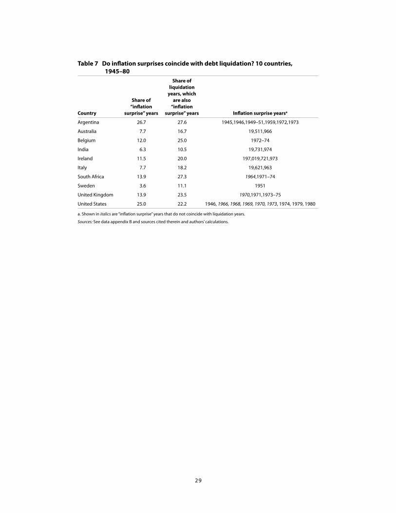
29
table 7 do inflation surprises coincide with debt liquidation? 10 countries, 1945–80
country
share of “inflation
surprise” years
share of liquidation
years, which are also
“inflation surprise” years Inflation surprise yearsa
Argentina 26.7 27.6 1945,1946,1949–51,1959,1972,1973
Australia 7.7 16.7 19,511,966
Belgium 12.0 25.0 1972–74
India 6.3 10.5 19,731,974
Ireland 11.5 20.0 197,019,721,973
Italy 7.7 18.2 19,621,963
South Africa 13.9 27.3 1964,1971–74
Sweden 3.6 11.1 1951
United Kingdom 13.9 23.5 1970,1971,1973–75
United States 25.0 22.2 1946, 1966, 1968, 1969, 1970, 1973, 1974, 1979, 1980
a. Shown in italics are “inflation surprise” years that do not coincide with liquidation years.
Sources: See data appendix B and sources cited therein and authors’ calculations.

30
32
Table 8 Inflation performance during major domestic public debt reduction episodes, 28 countries, 1790–2009
*A debt reduction episode is defined as a decline in the domestic public debt/GDP ratio over a three-year window. The dates shown are for the largest three-year declines recorded during the full sample period as shown in table A.3. Notes: The largest annual (single-year) decline recorded in debt/GDP is shown year shown in italics under the Dates column. For example, for Germany this was the hyperinflation year 1923; for the United States it was 1952, the year following a substantial debt conversion (see table 2).
Averag e Media n Average Medi anArgentina
1900-1902 ,1990,2006-20 07 479.8 8.2 82.5 8.6
Aust ralia 19 48,194 9 -1953 10 .3 9.3 3.0 2.5Belgium 1925-28 , 1949 10 .7 12.8 2.0 1.9Brazil 1990-199 2 ,1995-1996 898.2 9 80.2 111.3 11.3Canada 19 48,194 9 -1952 7.3 5.3 3.2 2.5Chile 1993 -1997, 2004-2007 7.7 6.1 17.7 5.5Colombia 20 08 , 2009 8.5 6.3 12.6 10.8Egy p t 2008 12 .0 8.6 11.7 9.9Finland 1946-1949 34 .5 24.9 10.4 3.9France 1924, 192 6-1927, 19 38 11 .1 12.6 6.4 2.7Germany 19 22, 1923 555504 9529.6 1764.7 231 460401.3 2.3Greece 192 5 -1927 23 .7 12.8 8.0 5.1India 1958 , 1996, 2006 7.1 6.2 6.6 6.2Ireland 1972, 1982 , 1998 9.8 8.6 5.9 3.7Italy 1945, 1946 -19 48 106.7 44.3 10.6 2.6Jap an 1898, 1912 -19 13 7.6 6.7 3.6 2.6Korea 1986 2.5 2.5 6.3 4.6M alay sia 1995 8.4 8.8 6.9 5.4M exico 1991, 1992 , 1993 18 .9 20.0 13.3 5.6New Zealand 1935-19 37 , 1950-1952 4.9 5.3 4.2 2.8Ph illip ines 1998, 2007 -20 08 7.2 7.7 7.7 6.2South Africa 193 5, 1952, 1981, 2001-
20027.0 6.6 5.8 4.9
Swed en 194 8, 1952, 1989, 2001 -200 3, 2009
4.7 3.2 4.4 3.2
Thailand 198 9-1990 4.4 4.6 4.8 3.8Turkey 19 43, 2006-2008 23 .2 9.2 25.3 9.7UK 1836, 1846, 1854, 19 36,
1940, 19 48-1950 ,1951-1954
4.7 3.7 2.7 1.8
US 1794-1796, 1881-1882, 1948-1952 , 1953, 19 57,
19664.0 2.6 1.6 1.7
Venezuela 1989, 1997 -1998, 20 06-2007
41 .6 29.5 11.4 5.8
Major D ebt Reduction Episodes * Ful l Sam ple
D atesInflation Inflation
table 8 Inflation performance during major domestic public debt reduction episodes, 28 countries, 1790–2009 (percent)
*A debt reduction episode is defined as a decline in the domestic public debt/GDP ratio over a three-year window. The dates shown are for the largest three-year declines recorded during the full sample period as shown in table A.3.
Notes: The largest annual (single-year) decline recorded in debt/GDP is shown in italics under the Dates column. For example, for Germany this was the hyperinflation year 1923; for the United States it was 1952, the year following a substantial debt conversion (see table 2).

31
Figure 1 surges in central government public debts and their resolution: Advanced and emerging-market economies, 1900–2011 (percentage points)
Notes: Listed in parentheses below each debt-surge episode are the main mechanisms for debt resolution besides fiscal austerity programs, which were not implemented in any discernible synchronous pattern across countries in any given episode. Specific default/restructuring years by country are provided in the Reinhart-Rogoff database and a richer level of detail for 1920s–1950s (including various conversions) are listed in table 1. The “typical” forms of financial repression measures are discussed in box 1 and greater detail for the core countries are provided in table 2.
Sources: Reinhart (2010), Reinhart and Rogoff (2009, 2011a), sources cited therein; authors’ calculations.
33
Figure 1 Surges in central government public debts and their resolution: Advanced and emerging-market economies, 1900–2011
Notes: Listed in parentheses below each debt-surge episode are the main mechanisms for debt resolution besides fiscal austerity programs, which were not implemented in any discernible synchronous pattern across countries in any given episode. Specific default/restructuring years by country are provided in the Reinhart-Rogoff database and a richer level of detail for 1920s–1950s (including various conversions) are listed in table 1. The “typical” forms of financial repression measures are discussed in box 1 and greater detail for the core countries are provided in table 2. Sources: Reinhart (2010), Reinhart and Rogoff (2009, 2011a), sources cited therein; authors’ calculations.
0
20
40
60
80
100
120
1901 1911 1921 1931 1941 1951 1961 1971 1981 1991 2001 2011
WWI and Depression debts(advanced economies:
default, restructuring and conversions--a few
hyperinflations)
Advanced economies
Emerging Markets
Great depression debts
(emerging markets-default)
WWII debts:(Axis countries: default and financial repression/inflation
Allies: financial repression/inflation)
1980s Debt Crisis(emerging
markets:default, restructuring, financial repression/inflation and several hyperinflations)
Second Great Contraction (advanced economies)

32
Figure 2 Average ex post real rate on treasury bills: Advanced and emerging-market economies, 1945–2009 (3-year moving averages, in percent)
Notes: The advanced-economy aggregate comprises Australia, Belgium, Canada, Finland, France, Germany, Greece, Ireland, Italy, Japan, New Zealand, Sweden, the United States, and the United Kingdom. The emerging-market group consists of Argentina, Brazil, Chile, Colombia, Egypt, India, Korea, Malaysia, Mexico, Philippines, South Africa, Turkey, and Venezuela. The average is unweighted and the country coverage is somewhat spotty prior to 1960 for emerging markets.
Sources: International Monetary Fund, International Financial Statistics; various sources listed in the data appendix B; and authors’ calculations.
34
Figure 2 Average ex post real rate on treasury bills: Advanced and emerging-market economies, 1945–2009 (3-year moving averages, in percent)
Notes: The advanced-economy aggregate comprises Australia, Belgium, Canada, Finland, France, Germany, Greece, Ireland, Italy, Japan, New Zealand, Sweden, the United States, and the United Kingdom. The emerging-market group consists of Argentina, Brazil, Chile, Colombia, Egypt, India, Korea, Malaysia, Mexico, Philippines, South Africa, Turkey, and Venezuela. The average is unweighted and the country coverage is somewhat spotty prior to 1960 for emerging market. Sources: International Monetary Fund, International Financial Statistics; various sources listed in the data appendix; and authors’ calculations.
1945-1980 1981-2009-1.6 2.8-1.2 2.6
Average Real Treasury Bill Rate
Advanced economiesEmerging markets
-15.0
-10.0
-5.0
0.0
5.0
10.01945 1950 1955 1960 1965 1970 1975 1980 1985 1990 1995 2000 2005 2010
`
Advanced economies (3-year moving average)
Emerging Markets (3-year moving average)
Financial Repression Era

33
Figure 3 Average ex post real discount rate: Advanced and emerging-market economies, 1945–2009 (3-year moving averages, in percent)
Notes: The advanced-economy aggregate comprises Australia, Belgium, Canada, Finland, France, Germany, Greece, Ireland, Italy, Japan, New Zealand, Sweden, the United States, and the United Kingdom. The emerging-market group consists of Argentina, Brazil, Chile, Colombia, Egypt, India, Korea, Malaysia, Mexico, Philippines, South Africa, Turkey, and Venezuela. The average is unweighted and the country coverage is somewhat spotty prior to 1960 for emerging markets.
Sources: International Monetary Fund, International Financial Statistics; various sources listed in the data appendix B; and authors’ calculations.
35
Figure 3 Average ex post real discount rate: Advanced and emerging-market economies, 1945–2009 (3-year moving averages, in percent)
Notes: The advanced-economy aggregate comprises Australia, Belgium, Canada, Finland, France, Germany, Greece, Ireland, Italy, Japan, New Zealand, Sweden, the United States, and the United Kingdom. The emerging-market group consists of Argentina, Brazil, Chile, Colombia, Egypt, India, Korea, Malaysia, Mexico, Philippines, South Africa, Turkey, and Venezuela. The average is unweighted and the country coverage is somewhat spotty prior to 1960 for emerging markets. Sources: International Monetary Fund, International Financial Statistics; various sources listed in the data appendix; and authors’ calculations.
1945-1980 1981-2009-1.1 2.7-5.3 3.8
Average Real Discount Rate
Advanced economiesEmerging markets
-20.0
-15.0
-10.0
-5.0
0.0
5.0
10.0
15.0
20.01945 1950 1955 1960 1965 1970 1975 1980 1985 1990 1995 2000 2005 2010
`
Advanced economies (3-year moving average)
Emerging Markets (3-year moving average)
Financial Repression Era

34
Figure 4 Average ex post real interest rates on deposits: Advanced and emerging-market economies, 1945–2009 (3-year moving averages, in percent)
Notes: The advanced-economy aggregate comprises Australia, Belgium, Canada, Finland, France, Germany, Greece, Ireland, Italy, Japan, New Zealand, Sweden, the United States, and the United Kingdom. The emerging-market group consists of Argentina, Brazil, Chile, Colombia, Egypt, India, Korea, Malaysia, Mexico, Philippines, South Africa, Turkey, and Venezuela. The average is unweighted and the country coverage is spotty prior to 1960.
Sources: International Monetary Fund, International Financial Statistics; various sources listed in the data appendix B; and authors’ calculations.
36
Figure 4 Average ex post real interest rates on deposits: Advanced and emerging-market economies, 1945–2009 (3-year moving averages, in percent)
Notes: The advanced-economy aggregate comprises Australia, Belgium, Canada, Finland, France, Germany, Greece, Ireland, Italy, Japan, New Zealand, Sweden, the United States, and the United Kingdom. The emerging-market group consists of Argentina, Brazil, Chile, Colombia, Egypt, India, Korea, Malaysia, Mexico, Philippines, South Africa, Turkey, and Venezuela. The average is unweighted and the country coverage is spotty prior to 1960. Sources: International Monetary Fund, International Financial Statistics; various sources listed in the data appendix; and authors’ calculations.
1945-1980 1981-2009-1.94 1.35-4.01 2.85
Average Real Interest Rate on Deposits
Advanced economiesEmerging markets
-15.0
-10.0
-5.0
0.0
5.0
10.01945 1950 1955 1960 1965 1970 1975 1980 1985 1990 1995 2000 2005 2010
`
Advanced economies (3-year moving average)
Emerging Markets (3-year moving average)
Financial Repression Era

35
Figure 5 real interest rate frequency distributions: Advanced economies, 1945–2009 (probability density function)
Source: Table B.3 in appendix B.
37
Figure 5 Real interest rate frequency distributions: Advanced economies, 1945–2009
a. Treasury bill rate
b. Discount rate
c. Deposit rate
1945-1980 1981-20090 46.9 10.5
1 percent 61.6 25.22 percent 78.6 36.23 percent 88.6 55.0
Real Interest rate on T-billsShare of obsevations at or below:
-0.2
1.8
3.8
5.8
7.8
9.8
11.8
13.8
15.8
17.8
19.8
-10 -9 -8 -7 -6 -5 -4 -3 -2 -1 0 1 2 3 4 5 6 7 8 9 10 11
1945-1980 1981-2009
1945-1980 1981-20090 41.9 11.6
1 percent 54.6 23.52 percent 69.4 37.03 percent 82.1 54.9
Real discount rateShare of obsevations at or below:
-0.2
1.8
3.8
5.8
7.8
9.8
11.8
13.8
15.8
17.8
19.8
-10 -9 -8 -7 -6 -5 -4 -3 -2 -1 0 1 2 3 4 5 6 7 8 9
1945-1980
1981-2009
1945-1980 1981-20090 58.8 24.6
1 percent 82.7 58.02 percent 94.7 85.43 percent 98.4 96.6
Real Interest rate on depositsShare of obsevations at or below:
-0.2
4.8
9.8
14.8
19.8
24.8
29.8
34.8
39.8
-10 -8 -6 -4 -2 0 2 4 6 8 10 12
1945-1980
1981-2009

36
Figure 6 real deposit interest rate frequency distributions, united kingdom, 1880–2010 (percentage points)
Sources: International Monetary Fund, International Financial Statistics; various sources listed in the data appendix B, and authors’ calculations.
38
Figure 6 Real deposit interest rate frequency distributions, United Kingdom, 1880–2010
Sources: International Monetary Fund, International Financial Statistics; various sources listed in the data appendix, and authors’ calculations.
0.0
0.1
0.2
0.3
0.4
0.5
0.6
-4 -2 0 2 4 6 8
1945-1980
1981-2010
1880-1939

37
APPendIx A. tABles And lIterAture revIew
table A.1 real interest rates during financial repression and post-liberalization
39
Appendix A. Tables and Literature Review
Table A.1 Real interest rates during financial repression and post-liberalization
Deposit Rate
Discount Rate
Interbank Rate
Lending Rate
T-Bill Rate
Before 23.99 -28.12After 0.97 -2.55Before -2.83 -0.64 -1.80 -0.04 -2.66After 2.61 3.86 3.83 6.98 3.46Before -0.50 1.29 -0.38 3.21 2.19After 1.75 4.14 3.68 6.94 2.96Before 18.69 0.58 -3.61 -0.21After 46.41 145.46 76.97 -21.87Before 2.07 -0.11 3.83 -0.65After 1.04 2.47 3.71 2.15Before 12.88 -12.49 28.39After 3.35 5.61 8.22Before -5.37 -3.64 -0.79After 6.14 7.72 11.04Before -5.65 -0.40 -1.43After 0.99 3.78 6.00Before -2.68 -2.83 1.43 -1.12After 1.46 2.94 4.00 4.51Before -3.09 -3.28 0.21 -0.46 -3.22After 1.33 4.92 4.58 5.70 3.20Before 0.94 0.69 1.11 3.92 0.60After 2.32 1.98 2.60 7.92 2.41Before 0.52 0.57 3.36 -1.88After 0.19 2.88 6.19 0.93Before 0.26 0.38 6.77After 1.11 1.45 5.86Before -4.02 0.04 -1.84 -1.52 -2.16After -1.11 4.12 3.13 3.57 2.84Before -3.30 -2.97 -1.44 1.47 -2.66After 0.94 4.70 3.59 6.22 3.32Before -2.13 -7.18 0.53 1.60 -1.61After 0.52 1.11 1.77 2.97 1.31Before 3.71 -1.71 5.19 3.38 7.94After 2.79 -0.56 3.75 3.93 4.08Before 1.86 1.05 -0.32 6.96 0.82After 1.90 1.87 1.72 5.35 1.57
1987
1992
1980
1983
1979
1991
1991
1980
1980
1989
1967
1984
1980
1991
1982
1984
1980
1980
(in percent)
Australia
Belgium*
Brazil
Canada
Argentina
Year of Liberalization
Average Real:
Chile
Colombia
Egypt
Finland
France
Germany*
Greece*
India
Ireland*
Italy
Japan
Korea
Malaysia
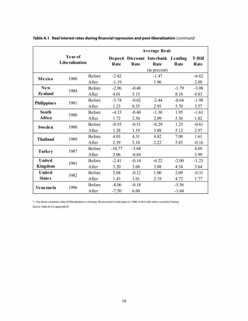
38
table A.1 real interest rates during financial repression and post-liberalization (continued)
* = For these countries, date of liberalization is missing. We assumed it took place in 1980, in line with other countries’ history.
Source: Table B.3 in appendix B.
40
Table A.1 Real interest rates during financial repression and post-liberalization(continued)
Deposit Rate
Discount Rate
Interbank Rate
Lending Rate
T-Bill Rate
Before -2.82 -1.47 -6.62After -1.19 1.96 2.88Before -2.96 -0.40 -1.79 -3.08After 4.01 5.15 8.18 4.83Before -3.74 -0.62 -2.44 -0.64 -1.98After 1.23 0.35 2.95 5.70 3.57Before -4.33 -0.40 -1.30 1.95 -1.61After 1.72 2.56 2.09 5.56 1.82Before -0.55 -0.51 -0.29 1.23 -0.61After 1.28 1.19 3.88 5.12 2.97Before 4.03 4.31 4.82 7.08 1.61After 2.39 3.10 2.22 5.83 -0.16Before -10.77 -3.68 4.69After 2.06 -0.84 3.99Before -2.41 -0.14 -6.22 -2.00 -1.23After 3.20 3.68 3.88 4.54 3.64Before 2.04 -0.12 1.00 2.09 -0.31After 1.43 1.61 2.19 4.72 1.77Before -8.06 -0.18 -5.56After -7.50 6.68 -1.64
1996
(in percent)
Year of Liberalization
Average Real:
1980
1989
1987
1981
1982
1988
1984
1981
1980
Turkey
United Kingdom
United States
Venezuela
Mexico
New Zealand
Philippines
South Africa
Sweden
Thailand

39
table A.2 measuring “taxes” from financial repression: selected papers
studymeasure(s) of financial
repression sample and coverage Highlight of findings
Agenor and Montiel (2008) End-of-year effective reserve requirements ratios are calcu-lated (see entry under Brock). The authors calculate how important a share of seignorage is accounted for by the reserve requirement tax.
32 advanced and emerging market economies 1980–1991.
Reserve ratios are higher for emerging markets. Among the advanced economies the highest share of seigniorage accounted for by reserve ratios is Italy over this period. For the emerging markets, Chile and Peru have the highest readings.
Beim and Calomiris (2001) Six measures (real interest rates, reserve ratio, liquidity, private borrowing, bank lending, and stock market capitalization) of financial repression are used to construct an aggregate index. Their aim is to provide a broad-brush cross-country comparison at a particular point in time—not a “tax equivalent” to the government.
All countries, advanced and emerging-market, data permit-ting. The most comprehensive coverage is for 1997. The annual indices are reported for 1970 and for 1990 for a subset of countries. The period of heaviest repression 1945–early 1970s is not part of the analysis.
Based on the cross-sectional evidence, the authors conclude that financial development (the opposite of repression) contrib-utes importantly to economic development and growth.
Brock (1989) End-of-year effective reserve requirements ratios are calculated as base money less currency in circulation (central bank reserves) divided broad money (or money plus quasi-money). Looks at the correlation between inflation rates and the reserve ratio.
41 advanced and emerging-market economies, 1960–84.
Reserve ratios are higher for emerging markets. Among the advanced economies these are highest for Australia and Italy over this period. A positive rela-tionship between inflation and reserve requirements is mostly present in the chronic high inflation countries of Africa and Latin America.
Easterly (1989) Net domestic transfers from the financial system and tax on financial intermediation. Uses inflation-adjusted flow of funds analysis to calculate the size of the transfers from reserve requirements, inflation tax, etc.
A dozen relatively large emerging markets. Flow-of-funds balance sheet from 1971 to1986.
Estimates are highest for Mexico and Yugoslavia among the 12 countries, reaching 12 to 16 percent of GDP in some years.
Easterly and Schmitt-Hebbel (1994)
Focus on real interest rates on deposits and calculate the repression tax revenue (from that source) as the difference between domestic rates and comparable rates in OECD countries multiplied by the end-of-period stock of deposits (the tax base).
Nine emerging markets, 1970–88 (the revenue calcula-tions are for less than half of the countries)
This component of the financial repression tax is in the order of 1 to 2 percent of GDP.
Giovannini and de Melo (1993) The effective interest rate on external (domestic) debt are calculated as the ratio of external (domestic) interest payments to the stock of external (domestic) debt. The government revenue from financial repression is calculated by computing the differential between the foreign borrowing cost and the domestic borrowing cost, times the average annual stock of domestic debt.
Roughly 1974–87 (usually shorter period), depending on the country. The 24- devel-oping-country sample does include Greece and Portugal as emerging markets.
Annual estimates of the “revenue from financial repression” are estimated from a low of 0.5 percent of GDP for Zaire (with its small domestic debt market to a high of about 6 percent for Mexico.
Estimates for Greece and Portugal are 2 to 2.5 percent of GDP.

40
Table A.2 sketches the approach, sample, and findings of six papers that have in different ways attempted
to quantify some of the dimensions of financial repression. While Beim and Calomiris (2001) primarily
aim to rank a cross-section of countries at a point (or two) in time to link the measures’ extent of
financial repression to growth and development, the remaining papers do attempt to quantify some of
the financial repression “revenue” equivalents. For instance, the papers dealing with reserve requirements
capture the tax on financial institutions. Ultimately (as Reinhart and Reinhart 1999 document) the banks
pass this tax on to depositors (via lower deposit rates), nongovernment borrowers (via higher lending
rates), or both, depending who has the most access to alternatives. If households are barred from holding
foreign assets and/or gold (see table 2), lower deposit rates are tolerated more readily. If domestic banks
are the only game in town for the firms, they will have to live with the higher lending rates.
The Giovannini and de Melo (1993) paper is closest in spirit to our fundamental two-part
intertwined question: (1) what is the annual saving on interest payments on domestic debt? and (2)
what is the magnitude of the erosion or liquidation on the existing stock of debt due to negative real
interest rates? Giovannini and de Melo (1993) compare “effective interest rates” on external debt to the
potentially repressed “effective interest rates on domestic debt” (see table A.1). This is a natural exercise
for emerging markets (the focus of their analysis) for the period that they consider (1974–87), as
emerging-market governments were funding themselves through both domestic and external borrowing
(in varying degrees), as documented by Reinhart and Rogoff (2011a). The market-determined interest
rate on external debt is a logical benchmark under such circumstances.
However, there are two compelling reasons why this approach is neither feasible nor desirable
for our purposes. First, some countries (like the United States and the Netherlands) do not have and
have not had historically external debt.34 All government debts are issued under domestic law and in
the domestic currency, irrespective of whether the holders of the debt are domestic pension funds or
foreign central banks. Second, most emerging markets had little or no external debt during the heyday
of the financial repression era during Bretton Woods (1945–73); the Depression of the 1930s and the
subsequent world war had all but eradicated global debt markets.
34. Apart from a trivial amount of Carter bonds in the 1970s, the US debt is domestic (homogenous) whether it is held by residents or nonresidents.

41
table A.3 extended sample for inflation and domestic debt reduction analysis, 28 countries, 1790–2009country sample period country sample period
Argentina 1884–2009 Italy 1914–2009
Australia 1914–2009 Japan 1885–1940, 1952–2009
Belgium 1920–39,1946–2009 Korea 1976–2005
Brazil 1900–2009 Malaysia 1955–57, 1976–2009
Canada 1925–2007 Mexico 1918–67, 1976–2009
Chile 1927–30,1937–53,1978–2009 New Zealand 1932–2008
Colombia 1923–2009 Philippines 1948–2009
Egypt 1993–2009 South Africa 1911–2009
Finland 1915–2009 Sweden 1880–2009
France 1920–38, 1949–2009 Thailand 1950–2009
Germany 1920–38, 1950–2009 Turkey 1933–72, 1976–2009
Greece 1920–39, 1950–65, 1978–81, 1993–2009 United Kingdom 1830–2009
India 1950–2009 United States 1790–2009
Ireland 1948–2008 Venezuela 1921–2009
Sources: Reinhart and Rogoff (2009, 2011a) and sources cited therein.

42
table B.1 structure of domestic government debt: coupon, maturity, bond prices, and tax revenuescountry Period covered source notes
Argentina 1944–74
1944–74
Ministerio de Hacienda
Banco Central de la República Argentina
Detailed composition of government debt is taken to indicate here as having data on: Outstanding debt stock (end of calendar or fiscal year) by coupon yield (instrument by instrument). Maturity of each instrument. In some cases it includes information on the marketable/nonmarketable distinction.
Tax revenues.
Prices of government bonds.
Australia 1945–68
19,711,976
Australia Bureau of Statistics
The Parliament of the Commonwealth of Australia
Detailed composition of government debt (see above).
Belgium 1945–74 Banque Nationale de Belgique Detailed composition of the government debt and bond prices.
Brazil 1964–93 Banco Central do Brasil
Series Historicas. Divida Publica
Estatisticas historicas do Brasil: series economicas, demograficas e sociais de 1550 a 1988–IBGE
Some debt data. Information on coefficient of monetary correction.
Debt data, maturity structure.
Tax revenues, GDP.
India 1949–80 Reserve Bank of India Detailed composition of the government debt, bond prices and tax revenues.
Ireland 1965–90
1965–90
Department of Finance
Central Statistics Office
Detailed debt data.
Tax revenues.
Italy 1945–70
1951–70
Istituto Centrale di Statistica
Banca d’Italia
Detailed composition of the government debt.
South Africa 1945–80 Control and Audit Office Detailed composition of the government debt and tax revenues.
Sweden 1945–65,
1984–90
Riksgaldskontoret
Fiscal Statistics for Sweden 1719–2003
Tax revenues.
United Kingdom 1945–80
1945–80
Bank of England
Central Statistical Office
Bond price data begins in 1960
Detailed composition of the government debt. Tax revenues
United States 1945–80
1945–80
Department of Treasury
Center for Research in Securities Prices (CRSP) database
Detailed composition of the debt, tax revenues.
Bond prices.
Source: Sbrancia (2011) and sources cited therein.
APPendIx B. dAtA APPendIx

43
table B.2 two examples of government debt profiles: India and the united statesa. India: composition of domestic debt for selected years, 1950–70 (as percent of total domestic debt)
component 1950 1960 1970
Marketable rupee loans 59 48 39
Treasury bills 15 25 21
Small savings 17 17 19
Other obligations 9 10 21
b. united states: composition of domestic debt for selected years, 1946–76 (as percent of total domestic debt)
component 1946 1956 1966 1976
Interest bearing obligations
Marketable obligations 67.3 58.0 65.8 64.5
Treasury bills 6.5 9.1 20.3 25.1
Certificates of indebtedness 11.4 6.9
Treasury notes 3.8 12.8 17.8 33.2
Treasury bonds 45.5 29.2 27.7 6.2
Other bonds 0.1 0 0 0
Nonmarketable obligations 22.7 24.7 16.7 35.4
Special issues 9.4 16.5 16.6 n.a.
Matured debt on which interest has ceased
0.2 0.3 0.1 0.1
Debt bearing no interest 0.4 0.6 0.8 0.1
Source: Sbrancia (2011) and sources cited therein.

44
Figure B.1 two examples of effective nominal interest rates on public debt: India and the united states (percent)
Source: Sbrancia (2011).
46
Figure B.1 Two examples of effective nominal interest rates on public debt: India and the United States
a. India, 1949–1980
b. United States, 1945–80
Source: Sbrancia (2011).
-15.0
-10.0
-5.0
0.0
5.0
10.0
15.0
20.0
25.0
30.0
1949 1954 1959 1964 1969 1974 1979
Inflation
Effective nominal interest rate on public debt
-0.1
1.9
3.9
5.9
7.9
9.9
11.9
13.9
1945 1950 1955 1960 1965 1970 1975 1980
Inflation
Effective nominal interest rate on public debt

45
table B.3 Interest rates: deposit, discount, lending, and treasury bill rates
(continued on next page)
47
Table B.3 Interest rates: Deposit, discount, lending, and treasury bill rates Country Interest Rate SourceArgentina Deposit Rate Banco Central de la Republica Argentina
Discount RateLending Rate
Australia Deposit Rate Reserve Bank of AustraliaDiscount RateLending RateT-Bill Rate
Belgium Deposit Rate Banque Nationale de BelgiqueDiscount RateLending RateT-Bill Rate
Brazil Deposit Rate Banco Central do BrasilDiscount RateLending RateT-Bill Rate
Canada Deposit Rate Bank of CanadaDiscount RateLending RateT-Bill Rate
Chile Deposit Rate Banco Central de ChileDiscount RateLending Rate
Colombia Deposit Rate Banco de la Republica de ColombiaDiscount RateLending Rate
Egypt Deposit Rate Central Bank of EgyptDiscount RateLending RateT-Bill Rate
Finland Deposit Rate Bank of FinlandDiscount RateLending Rate
France Deposit Rate Banque de FranceDiscount RateLending RateT-Bill Rate

46
table B.3 Interest rates: deposit, discount, lending, and treasury bill rates (continued)
(continued on next page)
48
Country Interest Rate SourceGermany Deposit Rate Deutsche Bundesbank
Discount RateLending RateT-Bill Rate
Greece Deposit Rate Bank of GreeceDiscount RateLending RateT-Bill Rate
India Discount Rate Reserve Bank of IndiaLending RateT-Bill Rate
Ireland Deposit Rate Central Bank of IrelandDiscount RateLending RateT-Bill Rate
Italy Deposit Rate Banca d'ItaliaDiscount RateLending RateT-Bill Rate
Japan Deposit Rate Bank of JapanDiscount RateLending RateT-Bill Rate
Korea Deposit Rate Bank of KoreaDiscount RateLending RateT-Bill Rate
Malaysia Deposit Rate Bank Negara MalaysiaDiscount RateLending RateT-Bill Rate
Mexico Deposit Rate Banco de MexicoLending RateT-Bill Rate
New Zealand Deposit Rate Reserve Bank of New ZealandDiscount RateLending RateT-Bill Rate

47
table B.3 Interest rates: deposit, discount, lending, and treasury bill rates (continued)
49
Country Interest Rate SourcePhilippines Deposit Rate Bangka Sentral Ng Pilipinas
Discount RateLending RateT-Bill Rate
South Africa Deposit Rate South Africa Reserve Bank Discount RateLending RateT-Bill Rate
Sweden Deposit Rate Sveriges RiksbankDiscount RateLending RateT-Bill Rate
Thailand Deposit Rate Bank of ThailandDiscount RateLending RateT-Bill Rate
Turkey Deposit Rate Turkiye Cumhuriyet Merkez BankasiDiscount RateT-Bill Rate
United Kingdom Deposit Rate Bank of EnglandDiscount RateLending RateT-Bill Rate
United States Deposit Rate Federal Reserve Bank of St. LouisDiscount RateLending RateT-Bill Rate Board of Governors of the Federal Reserve System
Venezuela Deposit Rate Banco Central de VenezuelaDiscount RateLending Rate