Working Paper No. 241

Optimal Financing by Money and Taxes of Productive and Unproductive Government Spending: Effects onEconomic Growth, Inflation, and Welfare

byDavid Alen Aschauer

I. Introduction

This paper contains an investigation of the effects of different means of financing government spending oneconomic growth, inflation, and welfare. In this setting, two different types of government spending areconsidered: productive expenditures which provide services to the private sector in its production activities;and unproductive expenditures which have no direct influence on the private economy. In turn, two differentforms of finance are considered: proportional income taxation; and money creation.

The primary result of the paper is, perhaps, striking in its simplicity. Specifically, we find that optimal publicfinance requires productive government expenditure to be financed by money creation and unproductivegovernment expenditure by income taxation. Within the model structure--a representative agent, endogenousgrowth model with money introduced via a cash-in-advance constraint--the basic result is robust to changes inthe values of all underlying model parameters such as the intertemporal elasticity of substitution inconsumption, the rate of time preference, and the output elasticity of public services.

The paper proceeds as follows. Section II contains a brief description of the model. Section III presents theeconomic equilibrium, while Sections IV and V compare the effects of financing productive and unproductiveexpenditures, respectively, by taxation and money creation. Section VI brings together the previous sectionsand considers the joint financing of government expenditures by taxation and money creation. Section VIIconcludes the paper and points to directions for future research.

II. Model Description

A. Modeling the Economy: Endogenous Growth

We are primarily concerned with the impact of government policies on the economy in the long run.Consequently, the analysis must revolve around a growth model in which such policies are capable of affectingeither the long run level of output or the long run growth rate of output. One candidate framework foranalysis is the neoclassical growth model of Solow (1956), in which growth is driven by exogenous factorssuch as population growth and technological change; another is the new growth model of Romer (1986), Lucas(1988), and Barro (1990), in which growth is determined endogenously. In the former model, a permanentchange in government policy is likely to have a permanent effect on the long run level of output, while in thelatter model such policy is likely to have a permanent effect on the long run rate of economic growth.

While the choice of the appropriate model is best determined by the available empirical evidence, such evidenceis fairly inconclusive. The empirical work in this area--which has burgeoned in recent years--tends to reject asimple form of the neoclassical growth model which focuses on physical capital accumulation, but is notincompatible with an "augmented" neoclassical growth model which, in addition, includes human capital (asin Mankiw, Romer, and Weil (1992)). Still, there is a strand of literature regarding the long run effects ofgovernment policy actions--particularly fiscal policies--which favors the endogenous growth model.Specifically, Kocherlakota and Yi (1996) show that permanent changes in certain forms of governmentexpenditures (e.g., education spending and physical capital spending) have an impact on long run economicgrowth. Using a different approach, Aschauer (1997) presents evidence that permanent changes in the stock of

public capital as well as changes in flow government spending affect the long run growth rate. We follow thisempirical literature and construct a endogenous growth model with government spending financed by taxationand money creation.

B. Modeling the Public Sector: Financing Productive and Unproductive Spending by Money Creation andTaxes

In recent research on the impact of public sector behavior on the economy, a number of authors have made acrucial distinction between productive and unproductive government expenditures. In particular, productiveexpenditures, such as education, research and development, job training, and physical infrastructure, are takento positively affect the efficiency of private sector production. On the theoretical front, Barro (1990) considersthe role of government spending in a simple endogenous growth model. His basic result is that productivegovernment spending, financed by a proportional income tax, will maximize economic growth and welfarewhen the output share of productive government spending, , is set equal to the output elasticity of suchspending, . In this context, either a lower ( < ) or higher ( > ) level of government spending acts as adrag on economic growth; in the former case because of insufficient government services, and in the latter casebecause of an excessive level of taxation. Turnovsky and Fisher (1995) investigate the composition ofgovernment expenditures and its consequences for macroeconomic performance in a neoclassical growthmodel. One of their main findings is that, to a first approximation, the marginal resource cost of productivegovernment spending (i.e., public infrastructure) should be set equal to unity (or its resource cost)--anotherway of stating the Barro rule of = .

There is a large and expanding literature on the empirical front as well. Aschauer (1989, 1990) initially broughtattention to the potential importance of public capital in private production, with estimates of the outputelasticity of public capital in the range of .35 to .40 in the United States over the post-World War II period.Later work has yielded mixed results. Lynde and Richmond (1993), Fernald (1993), Finn (1993), andKocherlakota and Yi (1996) obtain results which are generally supportive of Aschauer's original estimates,while others, such as Evans and Karras (1994), present findings which leave little or no room for a directpositive impact of public expenditures on private sector production.

In work which is particularly relevant to the analysis contained in the current paper, Aschauer (1997) uses datafor the U.S. states over the period from 1970 to 1990 and estimates the output elasticity of flow governmentexpenditures in a non-linear, endogenous growth model to be in the range of .04 and the output elasticity of thestock of public capital in the range of .33. We will follow these empirical results and assume that a significantportion of total government expenditures is of the productive form.

The total level of government expenditures needs to be financed in one fashion or another. In theabove-mentioned papers, when the method of financing is made explicit, government spending is typicallysupported by use of lump-sum or income taxation. The focus of attention in the present paper, however, is onthe relative importance of taxation and money creation in financing public expenditure. In a recent paper,Palivos and Yip (1995) carefully work out the effects of money versus tax finance of public expenditure in anendogenous growth model, but limit themselves to the case of unproductive government spending.1 We,instead, allow for both productive and unproductive government spending.

C. Modeling Money: The Cash-in-Advance Constraint

The main obstacle to rationalizing the holding of money by economic agents is that it is a rate of returndominated asset; other assets, such as bonds, yield a positive return and, therefore, are superior to money inacting as a store of value. Economists have devised a number of ways to overcome this obstacle in order tointroduce money into an economic model. For instance, in Sidrauski (1967), money is allowed to yield a directflow of utility services. In McCallum (1989) money is taken to reduce "shopping time" and, as a consequence,to increase leisure time. In the present model, we follow the cash-in-advance approach initiated by Clower(1967) which requires that the purchase of goods takes place through the use of money.

Once the cash-in-advance approach has been adopted as the method for introducing money into the analysis, abasic question arises: to what set of purchases should the constraint apply? In Lucas (1980), the set of

purchases is comprised of consumption goods; in Stockman (1981), the set of purchases includesconsumption and investment goods. The distinction between these two approaches is hardly withoutsignificance. In the former approach, the economy essentially dichotomizes into a real and monetary sector andmoney is superneutral--that is, changes in the growth rate of the money supply per se have no impact on therate of economic growth. In the latter approach, however, the real and monetary sectors become intertwined andchanges in the pace of money creation have an important effect on capital accumulation and economic growth.

One way of choosing between the two approaches is to look to the empirical evidence pertaining to the impactof money growth on long run economic growth. In an exhaustive analysis of 62 countries over the period from1979 to 1984, Dwyer and Hafer (1988) estimate a very small, though negative, relationship between real outputgrowth and money growth; specifically, in a univariate regression of real output growth on money growth, thecoefficient on the latter variable is estimated as -0.018 (s.e. .009). Thus, a 10 percentage point increase in themoney growth rate is estimated to modestly reduce annual economic growth from a sample average of .026 to.024. In a more recent analysis, Barro (1997) makes use of data for 109 countries over the period from 1960 to1990 and similarly finds a small effect of money growth and inflation on real output growth; in particular, a 10percentage point increase in the inflation rate is estimated to reduce the annual growth rate of per capita realoutput from a sample average of .022 to .020. Again, on purely statistical grounds, this relationship is ratherweak.

In light of this evidence, it would seem that the appropriate modeling strategy for this paper--which is pointedtoward an analysis of alternative government financing schemes in the long run and for a country such as theUnited States which, historically, has experienced a relatively low rate of inflation--is one in which money isessentially superneutral. As a consequence, we will assume that the cash-in-advance constraint applies toconsumption purchases and that, by implication, the financing of private investment purchases is accomplishedthrough the use of alternative credit instruments.

D. Model

We now describe, in equation form, the explicit model used in this paper. We assume an infinitely-livedrepresentative agent with preferences over current and future consumption given by

where u = utility, c = consumption, = a constant rate of time preference, and o -1 = a constant intertemporalelasticity of consumption.2 The agent seeks to maximize utility subject to a flow budget constraint as given by

where k = private capital, m = holdings of real money balances, y = output, T = a proportional tax rate onincome, Pi = the rate of price inflation, and a dot refers to a time derivative. Evidently, the agent may dispose ofafter-tax income by consuming, investing in capital, or by acquiring real money balances. In the present settingoutput is produced via the private sector production technology

where A = a productivity index and g p = productive government expenditures such as education, workertraining, research and development, and infrastructure. Labor input is taken to be inelastically supplied and isnormalized to unity--thereby equating output and output per worker. We follow Barro (1990) by assuming thatthe production function exhibits constant returns to scale in capital and productive public expenditures.

In addition to the budget constraint in (2) and the production technology in (3), the choices of therepresentative agent are limited by a cash-in-advance constraint

so that, in effect, the agent must have accumulated a sufficient level of real cash balances in order to consume ata particular level at any particular point in time.

The total level of government spending, g , is given by

where g u = unproductive government spending such as defense spending. Finally, the government budgetconstraint, which equates total government spending to the sum of the revenue from money creation and fromincome taxation, is

where µ = rate of monetary expansion and where we have combined the (potentially) separate budgetconstraints of the central bank and government treasury.

III. Equilibrium

The model equilibrium is attained through: solving the agent's problem of maximizing utility (1) subject to thebudget constraint (2) and the cash-in-advance constraint (3); manipulating the resulting first-order conditions;and, finally, imposing various market-clearing and balanced growth conditions. After these steps areaccomplished, the equilibrium is described by the following set of equations:

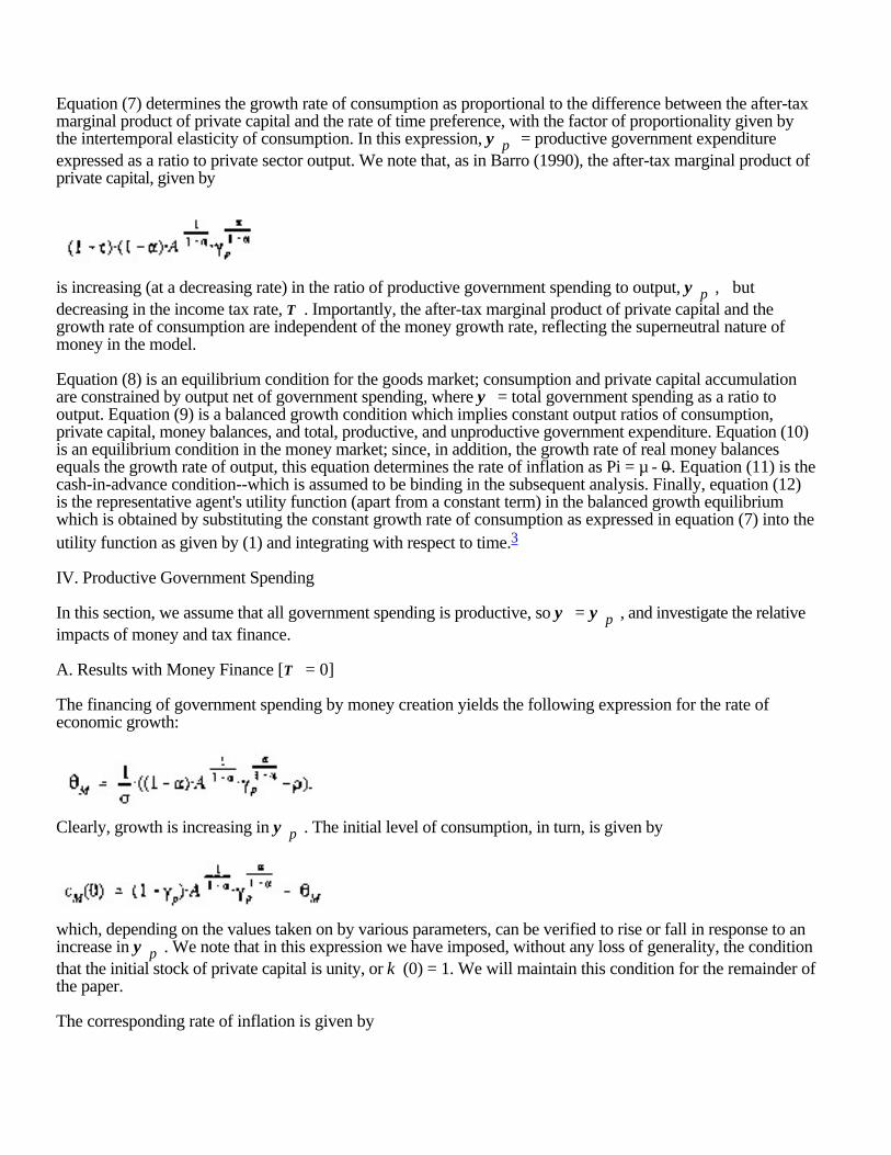
Equation (7) determines the growth rate of consumption as proportional to the difference between the after-taxmarginal product of private capital and the rate of time preference, with the factor of proportionality given bythe intertemporal elasticity of consumption. In this expression, y p = productive government expenditureexpressed as a ratio to private sector output. We note that, as in Barro (1990), the after-tax marginal product ofprivate capital, given by

is increasing (at a decreasing rate) in the ratio of productive government spending to output, y p , butdecreasing in the income tax rate, T . Importantly, the after-tax marginal product of private capital and thegrowth rate of consumption are independent of the money growth rate, reflecting the superneutral nature ofmoney in the model.

Equation (8) is an equilibrium condition for the goods market; consumption and private capital accumulationare constrained by output net of government spending, where y = total government spending as a ratio tooutput. Equation (9) is a balanced growth condition which implies constant output ratios of consumption,private capital, money balances, and total, productive, and unproductive government expenditure. Equation (10)is an equilibrium condition in the money market; since, in addition, the growth rate of real money balancesequals the growth rate of output, this equation determines the rate of inflation as Pi = µ - 0. Equation (11) is thecash-in-advance condition--which is assumed to be binding in the subsequent analysis. Finally, equation (12)is the representative agent's utility function (apart from a constant term) in the balanced growth equilibriumwhich is obtained by substituting the constant growth rate of consumption as expressed in equation (7) into theutility function as given by (1) and integrating with respect to time.3

IV. Productive Government Spending

In this section, we assume that all government spending is productive, so y = y p , and investigate the relativeimpacts of money and tax finance.

A. Results with Money Finance [T = 0]

The financing of government spending by money creation yields the following expression for the rate ofeconomic growth:

Clearly, growth is increasing in y p . The initial level of consumption, in turn, is given by

which, depending on the values taken on by various parameters, can be verified to rise or fall in response to anincrease in y p . We note that in this expression we have imposed, without any loss of generality, the conditionthat the initial stock of private capital is unity, or k (0) = 1. We will maintain this condition for the remainder ofthe paper.

The corresponding rate of inflation is given by

where the rate of money growth is determined as

Evidently, there are a variety of effects of an increase in y p on the rate of inflation. Note, in particular, that anincrease in government spending raises economic growth which, in turn, has an ambiguous effect on inflation.Given the money growth rate, a rise in output growth directly lowers the inflation rate. At the same time,however, the rise in output growth requires a shift in resources from consumption to investment which, in turn,has the effect of lowering the level of money balances and thereby necessitating a rise in the rate of moneygrowth to finance government spending. This latter effect raises the inflation rate.

Despite the fact that economic growth is increasing in y p , it is easily verified that the utility-maximizing valueof y p occurs where y p = a . To verify this point, we substitute c M (0), as given by equation (14), into therepresentative agent's utility function, as given by equation (12), and differentiate with respect to 0M to obtain

In this expression, c M (0) and (p - (1-ó)0M ) are assumed legitimately to be positive in order to ensure aneconomically meaningful equilibrium in which utility is positive (which rationalizes the former assumption) yetbounded (which rationalizes the latter assumption). Thus, since economic growth is increasing in y p , themaximization of utility requires y p be set equal to a .

B. Results with Tax Finance [µ = 0]

The financing of government spending by taxes requires T = y p and implies that economic growth is givenby

Here, economic growth is increasing in y p for y p < a , achieves a maximum at y p = a , and is decreasingin y p for y p > a . This finding, which extends that of Barro (1990) from a non-monetary to a monetarysetting, primarily arises as a result of the superneutral nature of money in the present model.

The initial level of consumption is given by

which, depending on the values of the various parameters of the model, may be an increasing or decreasingfunction of y p . The rate of inflation is given by

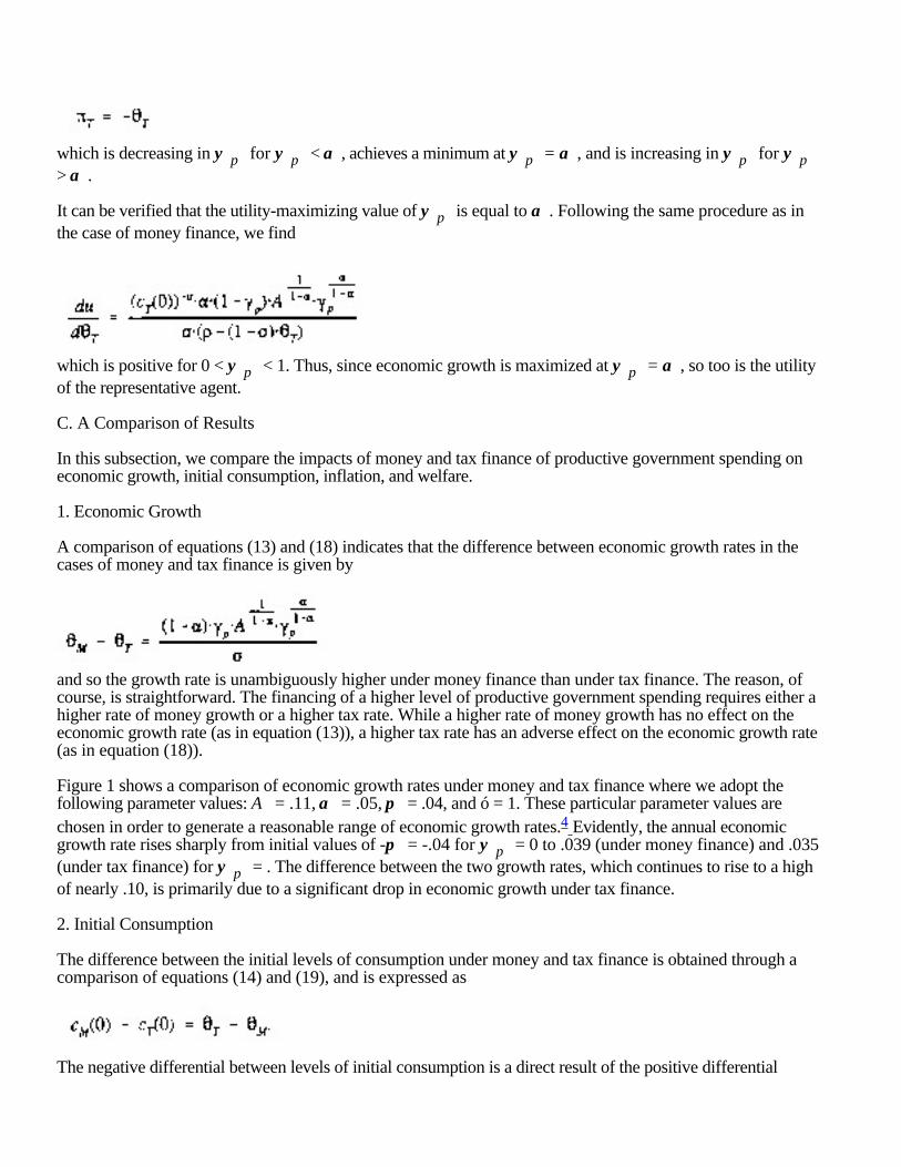
which is decreasing in y p for y p < a , achieves a minimum at y p = a , and is increasing in y p for y p> a .

It can be verified that the utility-maximizing value of y p is equal to a . Following the same procedure as inthe case of money finance, we find

which is positive for 0 < y p < 1. Thus, since economic growth is maximized at y p = a , so too is the utilityof the representative agent.

C. A Comparison of Results

In this subsection, we compare the impacts of money and tax finance of productive government spending oneconomic growth, initial consumption, inflation, and welfare.

1. Economic Growth

A comparison of equations (13) and (18) indicates that the difference between economic growth rates in thecases of money and tax finance is given by

and so the growth rate is unambiguously higher under money finance than under tax finance. The reason, ofcourse, is straightforward. The financing of a higher level of productive government spending requires either ahigher rate of money growth or a higher tax rate. While a higher rate of money growth has no effect on theeconomic growth rate (as in equation (13)), a higher tax rate has an adverse effect on the economic growth rate(as in equation (18)).

Figure 1 shows a comparison of economic growth rates under money and tax finance where we adopt thefollowing parameter values: A = .11, a = .05, p = .04, and ó = 1. These particular parameter values arechosen in order to generate a reasonable range of economic growth rates.4 Evidently, the annual economicgrowth rate rises sharply from initial values of -p = -.04 for y p = 0 to .039 (under money finance) and .035(under tax finance) for y p = . The difference between the two growth rates, which continues to rise to a highof nearly .10, is primarily due to a significant drop in economic growth under tax finance.

2. Initial Consumption

The difference between the initial levels of consumption under money and tax finance is obtained through acomparison of equations (14) and (19), and is expressed as

The negative differential between levels of initial consumption is a direct result of the positive differential

between rates of economic growth. Thus, we see that the choice between money and tax finance is ultimately achoice between current and future consumption; specifically, money finance is neutral with respect to thecurrent/future consumption mix, while tax finance favors current consumption by reducing the net return tocapital accumulation and the rate of economic growth.

3. Inflation

The difference between the inflation rates under money and tax finance can be shown to equal

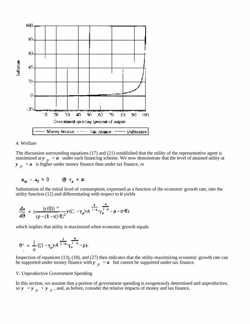
which, in general, takes on an ambiguous sign. For example, the inflation differential tends to be higher thelower the initial level of consumption or the lower the intertemporal elasticity of consumption. This is because ahigher level of productive government spending, under money finance, is then associated with a relatively lowlevel of real money balances and requires a relatively high rate of money creation to meet the requirements ofthe government budget constraint. However, for reasonable parameter values, the inflation differential ispositive and increasing in y p. Figure 2 indicates that an attempt to finance government spending throughmoney creation leads to a hyper-inflationary situation (defined here as an annual inflation rate in excess of1.00) for levels of government spending in excess of 50 percent of output.

Figure 1:Economic Growth under Money and Tax Finance

Figure 2:Inflation under Money and Tax Finance

4. Welfare

The discussion surrounding equations (17) and (21) established that the utility of the representative agent ismaximized at y p = a under each financing scheme. We now demonstrate that the level of attained utility aty p = a is higher under money finance than under tax finance, or

Substitution of the initial level of consumption, expressed as a function of the economic growth rate, into theutility function (12) and differentiating with respect to 0 yields

which implies that utility is maximized when economic growth equals

Inspection of equations (13), (18), and (27) then indicates that the utility-maximizing economic growth rate canbe supported under money finance with y p = a but cannot be supported under tax finance.

V. Unproductive Government Spending

In this section, we assume that a portion of government spending is exogenously determined and unproductive,so y = y p + y u , and, as before, consider the relative impacts of money and tax finance.

A. Results with Money Finance [T = 0]

The financing of government spending by money creation yields the following expression for the rate ofeconomic growth:

Clearly, growth is increasing in y p and is unaffected by y u . The initial level of consumption, in turn, isgiven by

which can be shown to rise or fall in response to an increase in y p and to fall in response to a rise in y u .The corresponding rate of inflation is given by

where the rate of money growth is determined as

As in the prior case, where all government spending was taken to be productive, there are a variety of effects ofan increase in y p on the rate of inflation. However, an increase in y u unambiguously raises the moneygrowth rate in equation (31) and, by implication, raises the inflation rate in equation (30).

It is straightforward to show that the utility-maximizing value of y p now occurs where y p = a - y u . Toverify this point, we substitute c M (0), as given by equation (29), into the representative agent's utilityfunction, as given by equation (12), and differentiate with respect to 0M to find:

For a given value of y u , the maximization of utility requires y be set equal to a , from which it follows thaty p be set equal to a - y u .

B. Results with Tax Finance [ó = 0]

The financing of government spending by taxes requires T = y and implies that economic growth is given by

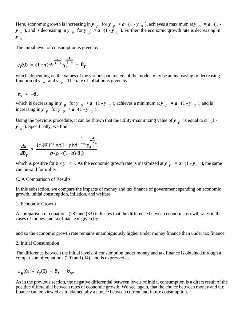
Here, economic growth is increasing in y p for y p < a ·(1 - y u ), achieves a maximum at y p = a ·(1 -y u ), and is decreasing in y p for y p > a ·(1 - y u ). Further, the economic growth rate is decreasing iny u .

The initial level of consumption is given by

which, depending on the values of the various parameters of the model, may be an increasing or decreasingfunction of y p and y u . The rate of inflation is given by

which is decreasing in y p for y p < a ·(1 - y u ), achieves a minimum at y p = a ·(1 - y u ), and isincreasing in y p for y p > a ·(1 - y u ).

Using the previous procedure, it can be shown that the utility-maximizing value of y p is equal to a ·(1 -y u ). Specifically, we find

which is positive for 0 < y < 1. As the economic growth rate is maximized at y p = a ·(1 - y u ), the samecan be said for utility.

C. A Comparison of Results

In this subsection, we compare the impacts of money and tax finance of government spending on economicgrowth, initial consumption, inflation, and welfare.

1. Economic Growth

A comparison of equations (28) and (33) indicates that the difference between economic growth rates in thecases of money and tax finance is given by

and so the economic growth rate remains unambiguously higher under money finance than under tax finance.

2. Initial Consumption

The difference between the initial levels of consumption under money and tax finance is obtained through acomparison of equations (29) and (34), and is expressed as

As in the previous section, the negative differential between levels of initial consumption is a direct result of thepositive differential between rates of economic growth. We see, again, that the choice between money and taxfinance can be viewed as fundamentally a choice between current and future consumption.

3. Inflation

The inflation rate differential under money and tax finance can be shown to equal

which duplicates equation (24), where government spending was limited to productive spending. Consequently,the inflation differential continues to take on an ambiguous sign without additional restrictions being placed onthe various model parameters.

4. Welfare

In general, the attained level of utility may be higher or lower under money than under tax finance ofgovernment expenditure. However, clear results can be established for two specific cases where we set the totallevel of government expenditure at a certain level of output, y = w .

(a) all government spending is productive, y u = 0, y p = a = w . This case is merely a restatement of theresults of the previous section. Money finance dominates tax finance in this case, and

(b) all government spending is unproductive, y u = w , y p = a = 0. Tax finance dominates money financein this case, and

To establish this result, we use the same procedure as in the previous section and differentiate the utilityfunction, expressed as a function of 0, to obtain

which implies that utility is maximized when economic growth equals

which can be supported under tax finance with T = w but not under money finance.

The reasoning behind the contrasting results in these two cases has been discussed by Barro (1990) andPalivos and Yip (1995). Government spending, whether productive (as in Barro (1990) in a model withoutmoney) or unproductive (as in Palivos and Yip (1995) in a model with money) involves an externality which,depending on the situation, may or may not need to be internalized by the use of taxes. The decision by therepresentative agent to increase (or decrease) private output by a unit carries with it the public sector responseof an increase (or decrease) in government spending by units. In the case of productive spending, with thegovernment setting the level of spending in an optimal fashion at y p = a = w , money finance yields theproper incentive, while tax finance yields too small an incentive, for capital accumulation and economic growth.In the case of unproductive spending, however, with y u = w , tax finance provides the appropriate incentive,while money finance provides too large an incentive, for investment and growth.

In between these two cases, there typically exists a range of values of productive and unproductive spending for

which money finance dominates tax finance and a range for which tax finance dominates money finance. Butthis leads to the likelihood that some combination of money and tax finance--rather than each alone-- willallow a higher level of welfare for the representative agent. We now investigate this possibility by consideringthe joint determination of money and tax financing of public expenditure.

VI. Joint Money and Tax Financing of Productive and Unproductive Spending

In this section, we determine the optimal structure of public sector spending and finance. In general, the rate ofeconomic growth and initial consumption are given by

We now assume that a certain fraction, Ø, of total government expenditure is financed by income taxation (withthe remainder financed by money creation) so that

Direct substitution of equation (46) into equations (44) and (45) and subsequent substitution of the resultingexpressions into the utility function (12) gives

Differentiation of equation (47) with respect to Ø and y p and equating the results to zero yields two firstorder conditions for utility maximization. The solution of these two equations then gives

so that the chosen level of productive government spending is proportional to the output elasticity of publicservices, and

so that the fraction of income taxation in total government revenue equals the fraction of unproductivegovernment spending in total government spending.

Making use of the government budget constraint, we then have

and

which is the central result of the paper: specifically, we find that optimal public finance requires productivegovernment spending to be financed by money creation and unproductive government spending by income

taxation.

Figure 3 shows contours of the utility function of the representative agent, equation (47), for the followingparameterization of the model: A = .11, a = .05, and y u = .05 as well as for various values of p and ó. Thebaseline case in panel (a) assumes p = .04 and ó = 1 and displays utility contours that are relatively symmetricaround the optimal values of ø = .5128 and y p = .0475. Panels (b) and (c) show the effect of varying theintertemporal elasticity of consumption, with respective values of equal to .5 and 2. Evidently, a decrease in theintertemporal elasticity of consumption (i.e., an increase in ó) tends to increase the importance of choosingthe correct level of productive government spending relative to the correct fraction of income taxation in totalrevenue. That is, the utility function becomes relatively steeper in the y p dimension (and relatively flatter inthe ø dimension) as ó increases. Panels (d) and (e) show the effect of varying the rate of time preference, withp respectively equal to .01 and .10. As with the (inverse) intertemporal elasticity of consumption, an increasein the rate of time preference tends to increase the relative importance of choosing the correct level ofproductive government spending.

In order to interpret the results obtained above, it is useful to focus on the partial problem of the optimal choiceof money and tax finance, given the optimal choice of the level of productive government spending.Accordingly, we set y p = a ·(1 - y u ) and T = ø·(y p + y u ) in equations (44) and (45) to obtain

and

It is then straight forward to verify that economic growth is decreasing in øand initial consumption is increasing in ø. In particular,

Figure 4 graphs h (·) and h c(·) for the baseline parameter values of the model. An increase in ø raises thelevel of consumption (relative to k (0) = 1) and lowers the economic growth rate and the associated level ofprivate investment. Once again, we note that the choice of finance is, in essence, a choice of present versusfuture consumption.

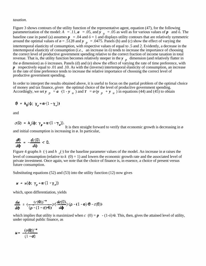
Substituting equations (52) and (53) into the utility function (12) now gives

which, upon differentiation, yields

which implies that utility is maximized when c (0) = p - (1-ó)·0. This, then, gives the attained level of utility,under optimal public finance, as

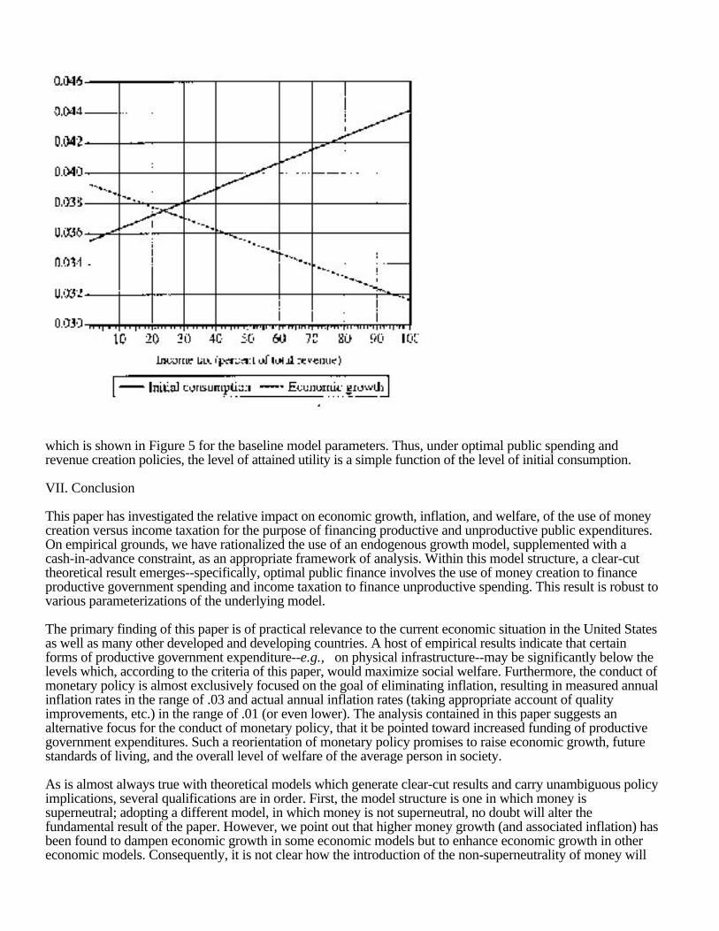
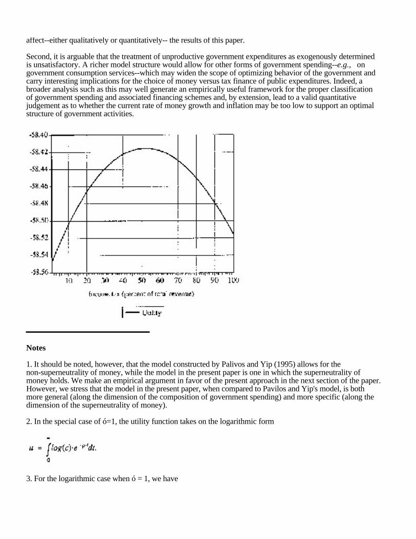
which is shown in Figure 5 for the baseline model parameters. Thus, under optimal public spending andrevenue creation policies, the level of attained utility is a simple function of the level of initial consumption.

VII. Conclusion

This paper has investigated the relative impact on economic growth, inflation, and welfare, of the use of moneycreation versus income taxation for the purpose of financing productive and unproductive public expenditures.On empirical grounds, we have rationalized the use of an endogenous growth model, supplemented with acash-in-advance constraint, as an appropriate framework of analysis. Within this model structure, a clear-cuttheoretical result emerges--specifically, optimal public finance involves the use of money creation to financeproductive government spending and income taxation to finance unproductive spending. This result is robust tovarious parameterizations of the underlying model.

The primary finding of this paper is of practical relevance to the current economic situation in the United Statesas well as many other developed and developing countries. A host of empirical results indicate that certainforms of productive government expenditure--e.g., on physical infrastructure--may be significantly below thelevels which, according to the criteria of this paper, would maximize social welfare. Furthermore, the conduct ofmonetary policy is almost exclusively focused on the goal of eliminating inflation, resulting in measured annualinflation rates in the range of .03 and actual annual inflation rates (taking appropriate account of qualityimprovements, etc.) in the range of .01 (or even lower). The analysis contained in this paper suggests analternative focus for the conduct of monetary policy, that it be pointed toward increased funding of productivegovernment expenditures. Such a reorientation of monetary policy promises to raise economic growth, futurestandards of living, and the overall level of welfare of the average person in society.

As is almost always true with theoretical models which generate clear-cut results and carry unambiguous policyimplications, several qualifications are in order. First, the model structure is one in which money issuperneutral; adopting a different model, in which money is not superneutral, no doubt will alter thefundamental result of the paper. However, we point out that higher money growth (and associated inflation) hasbeen found to dampen economic growth in some economic models but to enhance economic growth in othereconomic models. Consequently, it is not clear how the introduction of the non-superneutrality of money will

affect--either qualitatively or quantitatively-- the results of this paper.

Second, it is arguable that the treatment of unproductive government expenditures as exogenously determinedis unsatisfactory. A richer model structure would allow for other forms of government spending--e.g., ongovernment consumption services--which may widen the scope of optimizing behavior of the government andcarry interesting implications for the choice of money versus tax finance of public expenditures. Indeed, abroader analysis such as this may well generate an empirically useful framework for the proper classificationof government spending and associated financing schemes and, by extension, lead to a valid quantitativejudgement as to whether the current rate of money growth and inflation may be too low to support an optimalstructure of government activities.

Notes

1. It should be noted, however, that the model constructed by Palivos and Yip (1995) allows for thenon-superneutrality of money, while the model in the present paper is one in which the superneutrality ofmoney holds. We make an empirical argument in favor of the present approach in the next section of the paper.However, we stress that the model in the present paper, when compared to Pavilos and Yip's model, is bothmore general (along the dimension of the composition of government spending) and more specific (along thedimension of the superneutrality of money).

2. In the special case of ó=1, the utility function takes on the logarithmic form

3. For the logarithmic case when ó = 1, we have

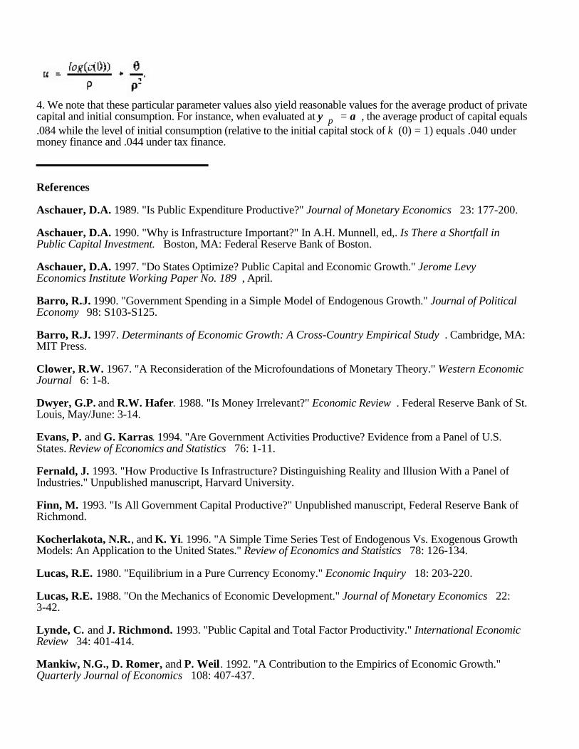
4. We note that these particular parameter values also yield reasonable values for the average product of privatecapital and initial consumption. For instance, when evaluated at y p = a , the average product of capital equals.084 while the level of initial consumption (relative to the initial capital stock of k (0) = 1) equals .040 undermoney finance and .044 under tax finance.

References

Aschauer, D.A. 1989. "Is Public Expenditure Productive?" Journal of Monetary Economics 23: 177-200.

Aschauer, D.A. 1990. "Why is Infrastructure Important?" In A.H. Munnell, ed,. Is There a Shortfall inPublic Capital Investment. Boston, MA: Federal Reserve Bank of Boston.

Aschauer, D.A. 1997. "Do States Optimize? Public Capital and Economic Growth." Jerome LevyEconomics Institute Working Paper No. 189 , April.

Barro, R.J. 1990. "Government Spending in a Simple Model of Endogenous Growth." Journal of PoliticalEconomy 98: S103-S125.

Barro, R.J. 1997. Determinants of Economic Growth: A Cross-Country Empirical Study . Cambridge, MA:MIT Press.

Clower, R.W. 1967. "A Reconsideration of the Microfoundations of Monetary Theory." Western EconomicJournal 6: 1-8.

Dwyer, G.P. and R.W. Hafer. 1988. "Is Money Irrelevant?" Economic Review . Federal Reserve Bank of St.Louis, May/June: 3-14.

Evans, P. and G. Karras. 1994. "Are Government Activities Productive? Evidence from a Panel of U.S.States. Review of Economics and Statistics 76: 1-11.

Fernald, J. 1993. "How Productive Is Infrastructure? Distinguishing Reality and Illusion With a Panel ofIndustries." Unpublished manuscript, Harvard University.

Finn, M. 1993. "Is All Government Capital Productive?" Unpublished manuscript, Federal Reserve Bank ofRichmond.

Kocherlakota, N.R., and K. Yi. 1996. "A Simple Time Series Test of Endogenous Vs. Exogenous GrowthModels: An Application to the United States." Review of Economics and Statistics 78: 126-134.

Lucas, R.E. 1980. "Equilibrium in a Pure Currency Economy." Economic Inquiry 18: 203-220.

Lucas, R.E. 1988. "On the Mechanics of Economic Development." Journal of Monetary Economics 22:3-42.

Lynde, C. and J. Richmond. 1993. "Public Capital and Total Factor Productivity." International EconomicReview 34: 401-414.

Mankiw, N.G., D. Romer, and P. Weil. 1992. "A Contribution to the Empirics of Economic Growth."Quarterly Journal of Economics 108: 407-437.

McCallum, B.T. 1989. Monetary Economics: Theory and Policy . New York, NY: Macmillan PublishingCompany.

Palivos, T. and C.K. Yip. 1995. "Government Expenditure Financing in an Endogenous Growth Model: AComparison." Journal of Money, Credit, and Banking 27: 1159-1178.

Romer, P.M. 1986. "Increasing Returns and Long-Run Growth." Journal of Political Economy 94:1002-1037.

Sidrauski, M. 1967. "Rational Choice and Patterns of Growth in a Monetary Economy." AmericanEconomic Review 57:534-544.

Solow, R.M. 1956. "A Contribution to the Theory of Economic Growth." Quarterly Journal of Economics70: 65-94.

Stockman, A.C. 1981. "Anticipated Inflation and the Capital Stock in a Cash-in-Advance Economy."Journal of Monetary Economics 8: 387-393.

Turnovsky, S.J. and W.H. Fisher. 1995. "The Composition of Government Expenditure and ItsConsequences for Macroeconomic Performance." Journal of Economic Dynamics and Control 19: 747-786.