5757 S. University Ave.

Chicago, IL 60637

Main: 773.702.5599

bfi.uchicago.edu

WORKING PAPER · NO. 2021-97

Financial Crises: A SurveyAmir Sufi and Alan M. TaylorAUGUST 2021

FINANCIAL CRISES:A SURVEY

Amir SufiAlan M. Taylor

August 2021

The authors thank Tobias Adrian, Matthew Baron, Ben Bernanke, Barry Eichengreen, Nicola Gennaioli, Robin Greenwood, Sam Hanson, Òscar Jordà, Hélène Rey, David Romer, Moritz Schularick, Andrei Shleifer, Emil Verner, and Wei Xiong, and especially our discussants, Maurice Obstfeld and Chenzi Xu, and editors, Gita Gopinath and Kenneth Rogoff, for feedback and suggestions. We thank Tyler Muir for kindly sharing data. Pranav Garg provided excellent research assistance. All errors are ours.

© 2021 by Amir Sufi and Alan M. Taylor. All rights reserved. Short sections of text, not to exceed two paragraphs, may be quoted without explicit permission provided that full credit, including © notice, is given to the source.

Financial crises: A surveyAmir Sufi and Alan M. Taylor August 2021JEL No. E32,E44,E7,G01,G10,N20

ABSTRACT

Financial crises have large deleterious effects on economic activity, and as such have been the focus of a large body of research. This study surveys the existing literature on financial crises, exploring how crises are measured, whether they are predictable, and why they are associated with economic contractions. Historical narrative techniques continue to form the backbone for measuring crises, but there have been exciting developments in using quantitative data as well. Crises are predictable with growth in credit and elevated asset prices playing an especially important role; recent research points convincingly to the importance of behavioral biases in explaining such predictability. The negative consequences of a crisis are due to both the crisis itself but also to the imbalances that precede a crisis. Crises do not occur randomly, and, as a result, an understanding of financial crises requires an investigation into the booms that precede them.

Amir SufiUniversity of ChicagoBooth School of Business5807 South Woodlawn AvenueChicago, IL 60637and NBERamir.sufi@chicagobooth.edu

Alan M. TaylorDepartment of Economics andGraduate School of ManagementUniversity of CaliforniaOne Shields AveDavis, CA 95616-8578and CEPRand also NBERamtaylor@ucdavis.edu

Contents

1 Introduction 1

2 Measurement: defining a financial crisis 62.1 Combining data and narrative criteria . . . . . . . . . . . . . . . . . . . . . . . 7

2.2 Standard binary classification . . . . . . . . . . . . . . . . . . . . . . . . . . . . 8

2.3 Finer classifications using narrative and data-driven criteria . . . . . . . . . . 13

3 Financial crisis predictability and causality 183.1 Credit expansion and asset price growth . . . . . . . . . . . . . . . . . . . . . 19

3.2 What causes the credit expansion? . . . . . . . . . . . . . . . . . . . . . . . . . 24

3.3 Behavioral biases, incentives, and predictability . . . . . . . . . . . . . . . . . 27

3.4 Triggers . . . . . . . . . . . . . . . . . . . . . . . . . . . . . . . . . . . . . . . . . 32

4 Explaining the painful consequences of a crisis 344.1 The crisis itself, or the boom that precedes it? . . . . . . . . . . . . . . . . . . 34

4.2 Not all credit booms are equal . . . . . . . . . . . . . . . . . . . . . . . . . . . 37

5 Open economy considerations 395.1 Borrowing from abroad? . . . . . . . . . . . . . . . . . . . . . . . . . . . . . . . 40

5.2 Crises and the Global Financial Cycle . . . . . . . . . . . . . . . . . . . . . . . 41

6 Open questions and future research 42

References 46

1. Introduction

Economists have recently become more engaged with the study of financial crises and withgood reason. As the 2008 Global Financial Crisis unfolded, the profession and the widerworld got an overdue reminder of the importance of these events, both in terms of theirhistoric tendency to recur over time, their capacity to strike rich as well as poor countries,and the deep and lasting damage they can inflict on economies, societies, and polities.

Just looking back now on the decade 2009–19 we have seen in many countries an after-math of sluggish recovery, stagnant real wages, persistent output gaps and unemployment,low investment, and deteriorating fiscal positions (IMF, 2018). And though not a focusof this paper, beyond purely macroeconomic outcomes we have seen patterns in financialcrises of broader social damage now, and in the past, as health suffered (Stuckler, Meissner,Fishback, Basu, and McKee, 2012; Parmar, Stavropoulou, and Ioannidis, 2016; Karanikolos,Heino, McKee, Stuckler, and Legido-Quigley, 2016), trust in institutions eroded (Stevensonand Wolfers, 2011), and political sentiments polarized (Funke, Schularick, and Trebesch,2016; Mian, Sufi, and Trebbi, 2014). Disturbing as such consequences were to many ob-servers in real time after 2008, advances in research have revealed that such phenomena arevery typical responses, with quantitative evidence dating back 100 years or more.

For financial crises to be seen as a distinct, important, and disastrous type of event, wemight first ask: how damaging are they? and how frequent? The associated downturns aremuch more adverse than a typical normal recession. We present a headline summary inTable 1. Using local projections (LPs, see Jorda, 2005), the deviation of real GDP per capitay is estimated h years after a crisis event. In the first two panels, the event is a crisis yearand the baseline is trend; in the last two panels the event is the peak of a financial recession(a crisis within ±2 years) and the baseline is a normal recession. To start, using the simplercrisis year definition, Table 1a shows that at a 6 year horizon, real GDP per capita is lowerby about 5%–6% following crises, relative to trend. Table 1b shows the result is not drivenby the great global crises, the synchronized distress in many countries seen in the interwardepression and the 2008 Global Financial Crisis. Next, aligning events using business cyclepeaks as in Jorda, Schularick, and Taylor (2013), Table 1c shows that over 6 years, real GDPper capita is lower by about 4% after financial peaks, relative to normal peaks. Table 1dshows this is also not driven global crises, with a deviation of about 3% still seen.1

Large growth costs motivate the study of financial crises, and similar large, persistentlosses are found in other studies (Bordo, Eichengreen, Klingebiel, and Martınez-Perıa, 2001;Cerra and Saxena, 2008; Reinhart and Rogoff, 2009b). However, the other key metric is

1Arguably, the baseline using normal recessions in the last two panels is a stricter test, as it compares acrisis scenario to a reference downturn period, not just the unconditional growth trend.

1

Table 1: Costs: the path of real GDP per capita after financial crises: crisis years and crisis peaks

The table shows local projections of cumulative log real GDP per capita yt+h – yt with indicators for financial crisis years (first two panels)and normal and financial recession peaks (last two panels) in advanced economies for the full non-war sample (1870–2015 ex. war) andalso excluding the great global crises (1870–1913 and 1946–2006 ex. war). Classifications as in Jorda, Schularick, and Taylor (2013). Datafrom latest JST dataset (R5). Authors’ calculation. See text. Standard errors in parentheses. ∗ p < 0.05, ∗∗ p < 0.01, ∗∗∗ p < 0.001.

(a) Deviation from trend after a crisis year

h = 1 h = 2 h = 3 h = 4 h = 5 h = 6

1(Crisis) −3.29∗∗∗ −4.38

∗∗∗ −5.01∗∗∗ −5.77

∗∗∗ −5.68∗∗∗ −5.69

∗∗

( 0.44 ) ( 0.53 ) ( 0.71 ) ( 0.88 ) ( 1.14 ) ( 1.54 )Observations 2049.00 2031.00 2013.00 1995.00 1977.00 1959.00

(b) Deviation from trend after a crisis year, ex. great global crises (1870–1913 & 1946–2006)

1(Crisis) −2.79∗∗∗ −3.93

∗∗∗ −5.04∗∗∗ −5.76

∗∗∗ −5.01∗∗∗ −5.55

∗∗

( 0.65 ) ( 0.82 ) ( 0.86 ) ( 1.05 ) ( 1.17 ) ( 1.61 )

Observations 1846.00 1846.00 1846.00 1846.00 1846.00 1846.00

(c) Deviation from normal recession trend after a crisis peak

1(Peak, financial) −0.75∗ −2.54

∗∗ −3.42∗∗∗ −3.76

∗∗ −3.86∗∗ −4.19

∗∗

( 0.30 ) ( 0.80 ) ( 0.84 ) ( 1.06 ) ( 1.17 ) ( 1.30 )

Observations 2032.00 2014.00 1996.00 1978.00 1960.00 1942.00

(d) Deviation from normal recession trend after a crisis peak, ex. great global crises (1870–1913 & 1946–2006)

1(Peak, financial) −0.31 −1.64 −2.51∗ −2.68

∗ −2.76∗ −3.01

( 0.44 ) ( 0.92 ) ( 0.93 ) ( 1.12 ) ( 1.10 ) ( 1.46 )

Observations 1829.00 1829.00 1829.00 1829.00 1829.00 1829.00

how frequently such crises are observed. Ultimately, to first order, the welfare costs ofany type of rare disaster will depend on frequency times expected loss per event (Barro,2006, 2009). In the JST data employed above, advanced economies experienced over 200

peacetime recession events since 1870 but one in four (25%) of these recessions were of thefinancial crisis type. Financial crisis events are the salient form disaster: more common thanwars, pandemics, and the like. The raw event frequency summary for the onset of financialcrises is given in Table 2, and it is also noteworthy that, despite the unusually calm periodfrom 1946 to 1970, when no financial crisis events were seen in advanced economies andvery few in emerging economies, the incidence of financial crisis recessions has been largein recent decades, and comparable to outcomes in the turbulent 1870 to 1939 period.

These stylized facts form the backdrop for macroeconomists studying financial crises.In this survey we provide detail about the definition of crisis events, as well as our abilityto predict them and document their consequences. We consider open issues and directionsfor future research. The rest of this introduction sets the scene and frames the discussion.

2

Table 2: Frequency: empirical probabilities of normal and financial crisis recessions

The table shows the frequency of normal and financial crisis recessions in advanced economies for various samples, based classificationsand data in Jorda, Schularick, and Taylor (2013). The sample in the final column is the overall peacetime sample period covered by theprevious columns. Authors’ calculation. See text.

Fraction of country-year observations with onset of recession type

1870–1913 1919–1938 1946–1972 1973–2008 Overall

Normal recessions 0.17 0.10 0.06 0.09 0.11

Financial crisis recessions 0.06 0.05 0.00 0.03 0.04

All recessions 0.23 0.16 0.06 0.12 0.15

Definition: what is a financial crisis? In section 2 of the paper we review the variousways of defining a financial crisis that have been adopted. By far the most commonly usedclassification method could be said to be a mix of narrative and quantitative, focusing onevents characterized by large-scale macro distress in the banking system, including theclosure or suspensions of a large fraction of the system and/or the need for substantialgovernment interventions to protect the system from acute failure. This approach datesback to definitions developed at the World Bank and IMF in the 1980s and 1990s, at firstprimarily for use in emerging markets and developing countries, but the idea has beenrefined over time to reduce subjectivity and increase the use of hard data (Caprio andKlingebiel, 1996; Laeven and Valencia, 2020).

Some key features of this approach are worth noting. It is typically used to construct abinary 0-1 indicator of a crisis, but nothing finer. It implicitly equates a financial crisis to abanking crisis, which may be historically sensible given dominant bank-centered financialsystems in the last 200 years, but this is not incontrovertible, especially in the U.S. case.And for the method to be truly objective it would require hard data on many covariatesto capture different dimensions of distress. But as one goes back in historical time, theapplication of these methods may inevitably lean more narrative and less quantitative, andpotentially more subjective, an unavoidable hazard when there is scant availability of harddata in the distant past to measure crisis intensity (Bordo, Eichengreen, Klingebiel, andMartınez-Perıa, 2001; Reinhart and Rogoff, 2009b; Schularick and Taylor, 2012).

Some other caveats will also warrant discussion. A measurement concern is that abinary classification is somewhat crude, and recent efforts have been made to developeither finer narrative classifications (Romer and Romer, 2017), or classifications augmentedby market data (Baron, Verner, and Xiong, 2021). Such metrics capture variations in crisisintensity but, limited to historical epochs with adequate supporting data, may never fullyreplace the standard indicator. Another concern is the confounding of financial crisis eventswith other types of crises, such as sovereign default crises and currency crises (Kaminsky

3

and Reinhart, 1999). It is important to take into consideration other types of crises whichare often coincident, especially in emerging markets.

An overarching result that emerges through this discussion is that the economic con-sequences of a financial crisis are negative and substantial, however a financial crisis ismeasured. The variations in the approach to measurement generate important debate inthe literature; however, the debate does not undermine this central conclusion.

Build-up: crisis prediction and causality We saw unconditional frequencies of crisesin Table 2. A naıve interpretation would be that of a random Bernoulli event driven byprobability draw. But this would be inappropriate if the risk of a crisis event were timevarying and, in particular, state dependent. This matters for the correct interpretation ofthe economic mechanisms that trigger crisis events.

At the risk of over simplification, two very different views, not necessarily mutuallyexclusive, can be discerned in the broader theoretical and empirical literatures. A purerandom-draw view is clearly aligned with the basic “rare disaster” models in macroeco-nomics (Barro, 2006, 2009). It is also implicit in multiple-equilibrium views of banks runs(Diamond and Dybvig, 1983) which are often associated with a banking crisis. Randomnessmay be the arrival of “news” such as a bad productivity level or growth draw (Gorton andOrdonez, 2019). Asset prices may then move, damaging debtor and intermediary balancesheets, with potential for amplification via financial accelerator mechanisms compared tonon-financial macro models (Bernanke, Gertler, and Gilchrist, 1999).

Alternatively, state dependence may be at work. In older, descriptive models keycandidates were—often coincident—credit booms and asset price bubbles (Kindleberger,1978; Minsky, 1986). These might be accompanied by overbuilding and malinvestment,stressed by the Austrian School (von Hayek, 1939; von Mises, 1949). This literature often putnon-rational beliefs or behavior at the center of the explanation for financial crises. However,many mechanisms can generate credit booms and asset price bubbles, and associated risks,even in rational models: for example, rational bubble models, incentive misalignments,government bailouts, heterogeneous beliefs, strategic complementarities, or pecuniaryexternalities arising from constraints in the financial system (Brunnermeier and Oehmke,2013; Farhi and Tirole, 2012; Aikman, Haldane, and Nelson, 2014; Davila and Korinek,2017). In behavioral models a sequence of optimism shocks, with extrapolation, might drivethe boom—via borrower credit demand or lender credit supply shocks, or both—only to belater undercut by a pessimism draw (Bordalo, Gennaioli, and Shleifer, 2018).

The empirical evidence we survey supports the view that financial crises are indeedpredictable, especially by credit and asset price growth. Support has also built up for the

4

view that deviations from rational expectations are an important component in explainingthis predictability. In general, the findings in the literature fit a broader trend in macroeco-nomics towards the study of the booms that precede economic downturns; or, as (Beaudry,Galizia, and Portier, 2020) put it, “putting the cycle back into business cycle analysis.”

Aftermath: consequences of crises The unconditional path of economies is more adverseafter a recession with an associated financial crisis. Various mechanisms could be at workhere, such as impairments to the financial system that lead to inefficient flows or allocationsof the supply of credit, or scars left by debt overhang on firms and/or households on theborrower side, all of which might depress aggregate demand and/or supply (Myers, 1977;Bernanke, 1983; Mian and Sufi, 2018).

The literature has made inquiries into the consequences of crises for a broad rangeof outcome variables, with conditional LPs, attention to robustness, and efforts to teaseout causal interpretations. An important identification problem is that factors causing afinancial crisis may also independently explain the severity of the economic downturnassociated with financial crises. Credit booms, for example, may distort the economytoward unproductive investment projects. They may also lead to debt overhang and weakgrowth even in the absence of a financial crisis. This identification problem has been atough nut to crack, but we note that the findings in the literature to date suggest thatboth factors, the preceding imbalances and the crisis itself, are important in explaining thepainful economic consequences. This is a fruitful avenue for future research, especiallygiven the importance to policy-makers.2

These findings also raise the question of why the factors that lead to financial crisesmay have negative consequences for growth. We discuss how research has identifiedhousehold debt, rather than business debt, as the most salient form of debt overhang, andmost dangerous for the probability of a crisis and future economic output, which helpsus discriminate among contending economic models and mechanisms (Jorda, Schularick,and Taylor, 2016; Mian, Sufi, and Verner, 2017). For example, we might draw a distinctionbetween credit that is designed to boost the productive capacity of the economy, and creditthat is designed to boost the consumption of final goods. This may help resolve a difficultquestion in the literature: in the long run, countries with higher private credit to GDP ratioshave higher per-capita income levels. But in the short-run, a rapid rise in credit portendseconomic difficulty. Perhaps the type of credit matters in explaining this discrepancy. Wediscuss this and other questions in the final section of the chapter.

2For example, in the aftermath of the Great Recession, there has been an active debate in the United Stateson whether policy achieved the correct balance between addressing the banking crisis and addressing thecollapse of house prices and household balance sheets.

5

2. Measurement: defining a financial crisis

At first glance, identifying financial crisis events may seem to be a rather straightforwardmatter, a case of “I know it when I see it.” We certainly have many well-documentedinstances of recognizable banking panics, stock market crashes, and other such eventsdating back several centuries. Historians, economists, and policymakers have recognizedsuch discrete events in qualitative terms for centuries, when trying to improve theory andpolicy prescriptions in the immediate aftermath (e.g., Thornton, 1802; Bagehot, 1873) orwhen retrospectively looking back to take stock of the broader array of such events acrosstime and space (e.g., Kindleberger, 1978; Grossman, 1994, 2010).

In modern quantitative research, more precise definitions have been sought as the basisfor comparable classifications in long and wide comprehensive panel databases. In linewith common usage, and reflecting the dominance of bank-based finance systems aroundthe world in the modern era, we keep a focus on the term financial crisis as meaning afinancial crisis in the banking sector, i.e., synonymous with systemically-large banking crises,like most authors (e.g., Bordo and Meissner, 2016). In this chapter, space dictates that wekeep to our narrow remit, and set aside other types of financial market disruptions such asstock market crashes, manias and bubbles in commodity or asset prices, default and debtcrises, and currency or exchange rate crises.3 Yet the broader macroeconomic implicationsof these other events appear, as yet, to be less clear and consequential compared to thevery severe damage now seen to be associated with banking crises, whether in advanced oremerging and developing economies (Reinhart and Rogoff, 2009b, 2013; Jorda, Schularick,and Taylor, 2013).

This section describes the main approaches to the problem of binary classificationfor the dates of financial crises. We start first with mostly-narrative indicators, where asystemically-large banking crisis is in most cases quite obvious, given sufficient scale. Theproblem is largely with borderline crises, where some judgement calls inevitably intrude,such as whether many banks or deposits were affected, or whether state interventionswere significant. Without hard data to ground such measurements, which is especially aproblem in the more distant past, such quibbles can account for most differences betweenthe multiple prevailing classifications currently in wide use. We then discuss how morerecently narrative binary indicators can be replaced with continuous measures of severityor augmented with financial real-time data to create more granular classifications—clearlya worthwhile aspiration, even if data availability hampers the scope of such efforts.

3Of course, many of these other phenomena have been widely studied and classified. See, e.g., Kindle-berger (1978); Eichengreen, Rose, and Wyplosz (1995); Kaminsky and Reinhart (1999); Garber (2000); Bordo,Eichengreen, Klingebiel, and Martınez-Perıa (2001); Reinhart and Rogoff (2009b); Laeven and Valencia (2020).

6

The extensive literature focused on the definition of a financial crisis may suggest moredisagreement than there really is. Over time, different sources have used more or lessstrict criteria, and inevitably some close calls can be quite subjective. That said, there isa consistent finding that financial crises are associated with a large decline in economicoutput, regardless of the precise manner in which crises are measured. For example, inthe case of 19th century U.S. banking panics, Jalil (2015) documents wide disagreementsin several sources, and then revisits primary historical documentation to revise the eventchronology and confirm the steep downturns associated with crisis events. Such deep dataconstruction and revision has underpinned progress in recent decades, and this importantwork should continue, as a consensus chronology of events will help us better identifyoutcomes and underlying mechanisms.

2.1. Combining data and narrative criteria

As recently as the 1990s comprehensive panel databases on banking crises did not exist.Seminal work at the World Bank by Caprio and Klingebiel (1996) documented over 100

bank insolvency events in 90 countries from the 1970s to the 1990s. However, detailedinformation was only available for 26 countries, e.g., the intensity of the crisis and itsresolution cost. Large crises afflicted 70%–90% of the banking system, but smaller crisescovering 20%–60% were also documented. Following quickly, others expanded the ideato more countries and as far back as 1870 (see, e.g., Kaminsky and Reinhart, 1999; Bordo,Eichengreen, Klingebiel, and Martınez-Perıa, 2001). Later, work at the IMF by Laeven andValencia (2008, 2020) helped refine the quantitative and subjective criteria. Their approach isnow the principal baseline used to declare a systemic banking crisis, so it is worth quotingthem at length so that we understand how a mix of data and narrative, or quantitative andsubjective, criteria are combined in the standard definition:

Under our definition, in a systemic banking crisis, a country’s corporate andfinancial sectors experience a large number of defaults and financial institutionsand corporations face great difficulties repaying contracts on time. As a result,non-performing loans increase sharply and all or most of the aggregate bankingsystem capital is exhausted. This situation may be accompanied by depressedasset prices (such as equity and real estate prices) on the heels of run-ups beforethe crisis, sharp increases in real interest rates, and a slowdown or reversal incapital flows. In some cases, the crisis is triggered by depositor runs on banks,though in most cases it is a general realization that systemically importantfinancial institutions are in distress.

7

Using this broad definition of a systemic banking crisis that combines quanti-tative data with some subjective assessment of the situation, we identify thestarting year of systemic banking crises around the world since the year 1970.Unlike prior work. . ., we exclude banking system distress events that affectedisolated banks but were not systemic in nature. As a cross-check on the timingof each crisis, we examine whether the crisis year coincides with deposit runs,the introduction of a deposit freeze or blanket guarantee, or extensive liquiditysupport or bank interventions. This way we are able to confirm about two-thirdsof the crisis dates. Alternatively, we require that it becomes apparent that thebanking system has a large proportion of nonperforming loans and that mostof its capital has been exhausted. This additional requirement applies to theremainder of crisis dates. (Laeven and Valencia, 2008, p. 5)

Recent classifications that broadly adhere to this mix of quantitative and subjectiveprinciples include those of Reinhart and Rogoff (2009b) and Schularick and Taylor (2012).The former also identified not only the start year of crises, but also duration; the latter alsowent on to develop a classification of recessions into normal and financial types based onthe proximity of the recession peak to the start of a financial crisis event (Jorda, Schularick,and Taylor, 2013). In this section, we will not explore those extensions but simply focus onthe start-year dating that is common to all classifications now in widespread use. It shouldbe understood that as one goes back in time the availability of quantitative details aboutany given event will fade, and so any classification is likely to get more subjective, andhence correlate less with other classifications, in the more distant past.

2.2. Standard binary classification

We can examine several influential binary classifications, using criteria like those discussedabove, to see how consistently financial crisis events have been classified using the mostwidely used methods to date. We split this discussion in two to reflect the different breadthand span of the datasets. We first consider three datasets that provide a long-narrow panelfor the advanced economies from 1870 to recent times (Bordo, Eichengreen, Klingebiel,and Martınez-Perıa, 2001; Reinhart and Rogoff, 2009b; Jorda, Schularick, and Taylor, 2017).We then turn to an alternate set of three datasets that provide a short-wide panel foradvanced and emerging economies from 1970 onwards (Bordo, Eichengreen, Klingebiel,and Martınez-Perıa, 2001; Reinhart and Rogoff, 2009b; Laeven and Valencia, 2020). Weshould also note that the overlap is often limited: for example, in the former case Reinhartand Rogoff (2009b) seek to document crises as far back as 1800, when others start in 1870 or

8

Figure 1: The long panel: advanced economy crisis coincidence, 1870–2016

The figure considers 3 classifications, one in each panel, and refers only to the common sample of all three datasets. For each classificationthe panel shows the frequency with which the other two classifications produce a coincident crisis event within 0,1, or 2 years. Note thatthe classifications differ in sample coverage and in the unconditional event frequency. See text.

0.67

0.74 0.740.72

0.81 0.81

0.1

.2.3

.4.5

.6.7

.8.9

1

BEKM crisis within RR crisis within±0y ±1y ±2y ±0y ±1y ±2y

JST classification

0.700.74 0.74

0.57

0.66 0.67

0.1

.2.3

.4.5

.6.7

.8.9

1

BEKM crisis within JST crisis within±0y ±1y ±2y ±0y ±1y ±2y

RR classification

0.67

0.740.77

0.88

0.930.94

0.1

.2.3

.4.5

.6.7

.8.9

1

JST crisis within RR crisis within±0y ±1y ±2y ±0y ±1y ±2y

BEKM classification

1880; in the latter case Laeven and Valencia (2020) cover a much wider range of emergingeconomies after 1970 compared to the others. We focus on areas of overlap in these setsof classifications to demonstrate the consistency of different methods, while highlightingsome divergences that emerge.

Crises in advanced economies since 1870 First we turn to the three long-narrow datasets,denoted respectively BEKM, RR, and JST (Bordo, Eichengreen, Klingebiel, and Martınez-Perıa, 2001; Reinhart and Rogoff, 2009b; Jorda, Schularick, and Taylor, 2017). From thesesources we draw a crisis onset indicator Crisisct marking the first year of a financial crisisevent. For this indicator, we first show measures of coherence in Figure 1 and raw eventclassification data in Figure 2.

First note that the datsets have different coverage: JST runs from 1870 to 2016, BEKMfrom 1880 to 1997, RR from 1870 to 2010. However, all three cover all 17 countries in JST,on which we focus. With that proviso, JST counts 90 crises, BEKM counts 69, and RRcounts 102 (frequencies are 3.6%, 3.4%, 4.3%). Thus RR declare significantly more crisisevents, meaning BEKM and JST are more strict.4 Also, since the BEKM sample is smaller itcounts fewer than JST. This is apparent from raw data in Figure 2, where more RR events

4However, in a later paper Reinhart and Rogoff (2014) constructed a new dataset, with a more strict set ofcrisis events which excludes smaller and likely non-systemic events.

9

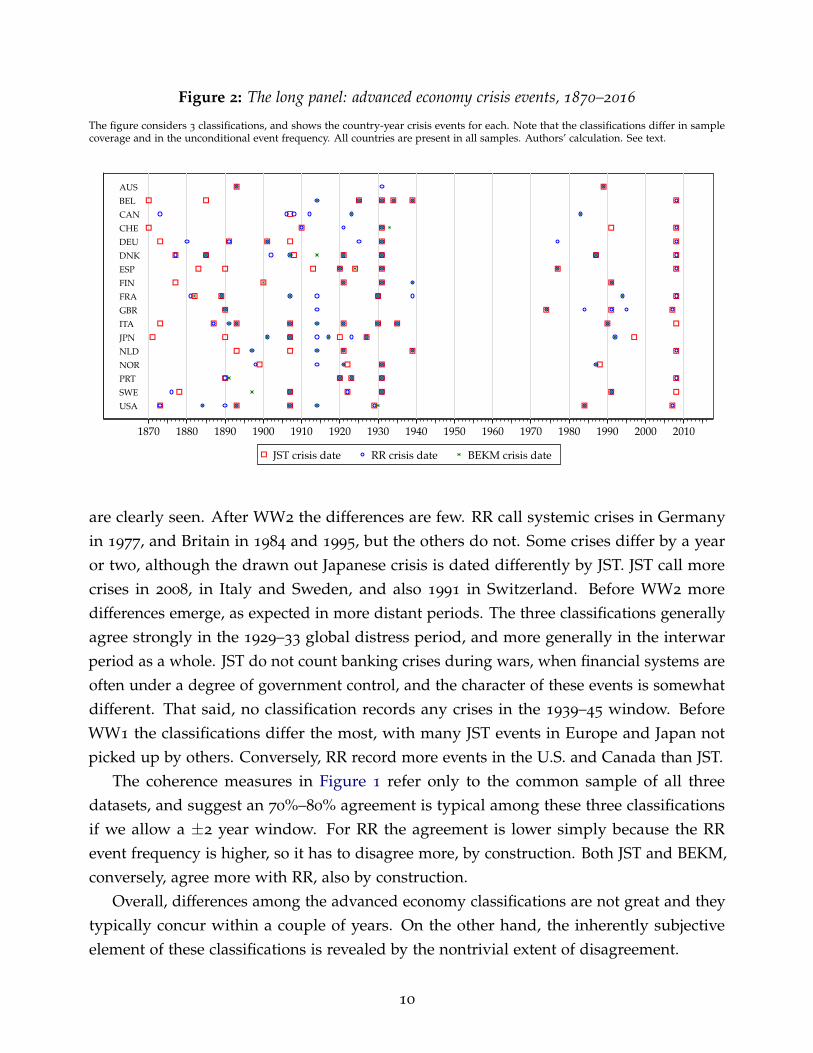
Figure 2: The long panel: advanced economy crisis events, 1870–2016

The figure considers 3 classifications, and shows the country-year crisis events for each. Note that the classifications differ in samplecoverage and in the unconditional event frequency. All countries are present in all samples. Authors’ calculation. See text.

USA

GBR

BEL

DNK

FRA

DEU

ITA

NLDNOR

SWE

CHECAN

JPN

FIN

PRT

ESP

AUS

1870 1880 1890 1900 1910 1920 1930 1940 1950 1960 1970 1980 1990 2000 2010

JST crisis date RR crisis date BEKM crisis date

are clearly seen. After WW2 the differences are few. RR call systemic crises in Germanyin 1977, and Britain in 1984 and 1995, but the others do not. Some crises differ by a yearor two, although the drawn out Japanese crisis is dated differently by JST. JST call morecrises in 2008, in Italy and Sweden, and also 1991 in Switzerland. Before WW2 moredifferences emerge, as expected in more distant periods. The three classifications generallyagree strongly in the 1929–33 global distress period, and more generally in the interwarperiod as a whole. JST do not count banking crises during wars, when financial systems areoften under a degree of government control, and the character of these events is somewhatdifferent. That said, no classification records any crises in the 1939–45 window. BeforeWW1 the classifications differ the most, with many JST events in Europe and Japan notpicked up by others. Conversely, RR record more events in the U.S. and Canada than JST.

The coherence measures in Figure 1 refer only to the common sample of all threedatasets, and suggest an 70%–80% agreement is typical among these three classificationsif we allow a ±2 year window. For RR the agreement is lower simply because the RRevent frequency is higher, so it has to disagree more, by construction. Both JST and BEKM,conversely, agree more with RR, also by construction.

Overall, differences among the advanced economy classifications are not great and theytypically concur within a couple of years. On the other hand, the inherently subjectiveelement of these classifications is revealed by the nontrivial extent of disagreement.

10

Figure 3: The short panel: advanced and emerging economy crisis coincidence, 1970–2016

The figure considers 3 classifications, one in each panel, and refers only to the common sample of all three datasets. For each classificationthe panel shows the frequency with which the other two classifications produce a coincident crisis event within 0,1, or 2 years. Note thatthe classifications differ in sample coverage and in the unconditional event frequency. Authors’ calculation. See text.

0.82

0.89 0.89

0.71

0.870.89

0.1

.2.3

.4.5

.6.7

.8.9

1

BEKM crisis within RR crisis within±0y ±1y ±2y ±0y ±1y ±2y

LV classification

0.70

0.780.81

0.39

0.480.49

0.1

.2.3

.4.5

.6.7

.8.9

1

BEKM crisis within LV crisis within±0y ±1y ±2y ±0y ±1y ±2y

RR classification

0.54

0.60 0.60

0.84

0.950.96

0.1

.2.3

.4.5

.6.7

.8.9

1

LV crisis within RR crisis within±0y ±1y ±2y ±0y ±1y ±2y

BEKM classification

Crises in advanced and emerging economies since 1970 The availability of historicaldata for emerging markets is more limited and this means that classification datasets heretake the form of short-wide panels, typically starting around 1970 and running up to thepresent. This was true for pioneering studies (Caprio and Klingebiel, 1996; Kaminsky andReinhart, 1999; Bordo, Eichengreen, Klingebiel, and Martınez-Perıa, 2001), although the RRdataset covers a more limited range of emerging markets all the way back to 1800, takinginto account any relevant date of independence.

For our purposes we will compare three datasets that run from 1970 onwards, andwhich span advanced and emerging economies: namely BEKM and RR, plus the additionof LV, denoting Laeven and Valencia (2020). We show measures of coherence in Figure 3

and raw event classification data in Figure 4.First note that the wide datasets have different coverage in this window: LV runs from

1970 to 2017, BEKM from 1973 to 1997, RR from 1970 to 2010. In addition, BEKM and RRcover a subset of less than half the countries spanned by the newer LV dataset. With thatnoted, we find that LV counts 151 crises, BEKM counts 62, and RR counts 120 (frequenciesare 1.9%, 4.2%, 4.3%). Thus from a frequency perspective, LV have a tendency to declaresignificantly fewer crisis events. This may reflect a stricter definition being used, or itmight just be that their larger sample, with many more emerging economies, contains fewerfinancially fragile (or, more financially repressed) economies. These patterns can also be

11

Figure 4: The short panel: advanced and emerging economy crisis events, 1970–2016

The figure considers 3 classifications, and shows the country-year crisis events for each. Note that the classifications differ in samplecoverage and in the unconditional event frequency, and overlap is limited. All countries are present in LV sample, other samples aredenoted by RR and BEKM in brackets on the right axis. Authors’ calculation. See text.

ALBANIAALGERIAANGOLAARGENTINA [RR BEKM]ARMENIAAUSTRALIA [RR BEKM]AUSTRIA [BEKM]AZERBAIJANBANGLADESH [BEKM]BARBADOSBELARUSBELGIUM [RR BEKM]BELIZEBENINBHUTANBOLIVIABOSNIA AND HERZEGOVINABOTSWANABRAZIL [RR BEKM]BRUNEIBULGARIABURKINA FASOBURUNDICAMBODIACAMEROONCANADA [RR BEKM]CAPE VERDECENT. AFR. REP.CHADCHILE [RR BEKM]CHINACOLOMBIA [RR BEKM]COMOROSCONGO, DEM. REP. OFCONGO, REP. OFCOSTA RICA [RR BEKM]COTE D'IVOIRE [RR BEKM]CROATIACYPRUSCZECH REPUBLICDENMARK [RR BEKM]DJIBOUTIDOMINICADOMINICAN REP.ECUADOR [RR BEKM]EGYPT [RR BEKM]EL SALVADOREQUATORIAL GUINEAERITREAESTONIAETHIOPIAFIJIFINLAND [RR BEKM]FRANCE [RR BEKM]GABONGAMBIA, THEGEORGIAGERMANY [RR BEKM]GHANA [RR BEKM]GREECE [RR BEKM]GRENADAGUATEMALAGUINEAGUINEA-BISSAUGUYANAHAITIHONDURASHONG KONG [BEKM]HUNGARYICELAND [RR BEKM]INDIA [RR BEKM]INDONESIA [RR BEKM]IRAN, I.R. OFIRELAND [RR BEKM]ISRAEL [BEKM]ITALY [RR BEKM]JAMAICA [BEKM]JAPAN [RR BEKM]JORDANKAZAKHSTANKENYAKOREA [RR BEKM]KUWAITKYRGYZ REPUBLICLAO PEOPLE’S DEM. REP.LATVIALEBANONLESOTHOLIBERIALIBYALITHUANIALUXEMBOURGMACEDONIAMADAGASCARMALAWIMALAYSIA [RR BEKM]MALDIVESMALIMAURITANIAMAURITIUSMEXICO [RR BEKM]MOLDOVAMONGOLIAMOROCCOMOZAMBIQUEMYANMARNAMIBIANEPALNETHERLANDS [RR BEKM]NEW CALEDONIANEW ZEALAND [RR BEKM]NICARAGUANIGERNIGERIA [RR BEKM]NORWAY [RR BEKM]PAKISTAN [BEKM]PANAMAPAPUA NEW GUINEAPARAGUAY [RR BEKM]PERU [RR BEKM]PHILIPPINES [RR BEKM]POLANDPORTUGAL [RR BEKM]ROMANIARUSSIARWANDASAO TOME AND PRINCIPESENEGAL [BEKM]SERBIA, REPUBLIC OFSEYCHELLESSIERRA LEONESINGAPORE [RR BEKM]SLOVAK REPUBLICSLOVENIASOUTH AFRICA [RR BEKM]SOUTH SUDANSPAIN [RR BEKM]SRI LANKA [RR BEKM]ST. KITTS AND NEVISSUDANSURINAMESWAZILANDSWEDEN [RR BEKM]SWITZERLAND [RR BEKM]SYRIAN ARAB REPUBLICTAJIKISTANTANZANIATHAILAND [RR BEKM]TOGOTRINIDAD AND TOBAGOTUNISIATURKEY [RR BEKM]TURKMENISTANUGANDAUKRAINEUNITED KINGDOM [RR BEKM]UNITED STATES [RR BEKM]URUGUAY [RR BEKM]UZBEKISTANVENEZUELA [RR BEKM]VIETNAMYEMENYUGOSLAVIA, SFRZAMBIAZIMBABWE [RR BEKM]

1970 1980 1990 2000 2010

LV crisis date RR crisis date BEKM crisis date

12

gleaned from Figure 4, where the raw data are shown. The coherence measures in Figure 3

again refer only to the common sample of all three datasets, and suggest an 80%–90%agreement is typical among these three classifications if we allow a ±2 year window. Theexception is the lower level of overlap from BEKM and RR crises when looking for a nearbyLV crisis, but given the much lower event frequency in the LV dataset this is entirely to beexpected. Overall, that apart, coherence is a little higher than in the long panel of advancedeconomies, perhaps suggesting slightly less subjectivity in more recent years.

Ending on a positive note, in the last 30 years the systematic classification of financialcrisis events has progressed from essentially nothing to a consensus approach with broadcoverage. Established databases now extend to many countries, cover most of the recentdecades for the entire world and even stretch back into the 1800s for a wide panel. Theymay disagree on certain specific historical events given the sometimes subjective judgementsinvolved, but agreement on the same criteria results in substantial overlap.

2.3. Finer classifications using narrative and data-driven criteria

From a theoretical perspective some might have the hope, possibly forlorn, that withsufficient detail the range of crisis outcomes can be encompassed as a continuum ofendogenously modeled distress, rather than as a separate regime in a more complexnonlinear or state-dependent world.

From that standpoint, the above binary classifications may be seen as lacking nuance,having no granular detail to allow the researcher to discriminate between more or lesssevere events. An intense financial crisis is coded as 1, but so are much milder crises. Wewould expect these differences to matter when analyzing causes and consequences.

Some recent progress has been made filling this gap using both narratives and data.

Finer classification using narrative criteria One way to make a finer classification is toparse narrative records more carefully, sorting events in to more than just two bins, on andoff as in Romer and Romer (2017). They built semiannual series on financial distress in 24

advanced countries for the period 1967–2012, using the OECD Economic Outlook. They basejudgements on accounts of the health of countries’ financial systems and classify distresswith an indicator F on a 16-bin scale, where 0 means no distress.

Using LP methods, a key finding is that, sensibly, higher levels of distress Fct, in country cat time t, are associated with slower growth going forward, as well as higher unemploymentand lower industrial production. A typical local projection for the cumulative real GDP

13

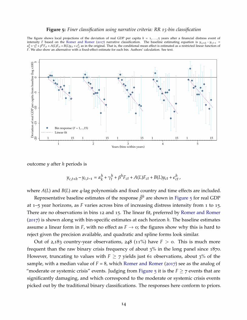
Figure 5: Finer classification using narrative criteria: RR 15-bin classification

The figure shows local projections of the deviation of real GDP per capita h = 1, . . . , 5 years after a financial distress event ofintensity F based on the Romer and Romer (2017) narrative classification. The baseline estimating equation is yc,t+h – yc,t–1 =αh

k + γht + βhFct + A(L)Fct + B(L)yct + ϵh

ct as in the original. That is, the conditional mean effect is estimated as a restricted linear function ofF. We also show an alternative with a fixed-effect estimate for each bin. Authors’ calculation. See text.

1 15 1 15 1 15 1 15 1 15-20

-15

-10

-50

5D

evia

tion

of r

eal G

DP

per

capi

ta fr

om b

asel

ine

(log

x100

)

1 2 3 4 5Years (bins within years)

Bin response (F = 1,...,15)Linear fit

outcome y after h periods is

yc,t+h – yc,t–1 = αhk + γh

t + βhFct + A(L)Fct + B(L)yct + ϵhct ,

where A(L) and B(L) are 4-lag polynomials and fixed country and time effects are included.Representative baseline estimates of the response βh are shown in Figure 5 for real GDP

at 1–5 year horizons, as F varies across bins of increasing distress intensity from 1 to 15.There are no observations in bins 12 and 15. The linear fit, preferred by Romer and Romer(2017) is shown along with bin-specific estimates at each horizon h. The baseline estimatesassume a linear form in F, with no effect as F → 0; the figures show why this is hard toreject given the precision available, and quadratic and spline forms look similar.

Out of 2,183 country-year observations, 248 (11%) have F > 0. This is much morefrequent than the raw binary crisis frequency of about 3% in the long panel since 1870.However, truncating to values with F ≥ 7 yields just 61 observations, about 3% of thesample, with a median value of F = 8, which Romer and Romer (2017) see as the analog of“moderate or systemic crisis” events. Judging from Figure 5 it is the F ≥ 7 events that aresignificantly damaging, and which correspond to the moderate or systemic crisis eventspicked out by the traditional binary classifications. The responses here conform to priors.

14

They are uncannily close to the Jorda, Schularick, and Taylor (2013) estimates, and thesummary estimates shown in Table 1, even though these estimates allow variable distressF = 0 across periods.5

Finer classification using data-driven criteria An alternative route to a finer classificationis to use observable financial data to infer stress in the financial system. In principle, thiscould produce crisis indicator completely divorced from qualitative or narrative information.This might be a valuable a step if some narrative events suffer from categorization bias, forexample, if an historical event is more likely to be classified by the observer as a systemiccrisis when it happens to be followed by a bad downturn, leading to spurious inferences.

An example of a data-augmented classification is Baron, Verner, and Xiong (2021), whomeasure the health of the banking system for 46 countries for the years 1870–2016, includingboth advanced and emerging countries. They propose that: “As there is no single correctdefinition of a banking crisis, our goal is to provide one possible construction of clear-cutcrisis episodes based on three systematic measures: bank equity declines, bank failures,and panics.” They collect market data on the first, and build new narrative indicators ofthe latter two, building on prior work.

In particular, they use bank equity declines to adjust earlier narrative lists. BVX refer toadditions as “forgotten” and deletions as “spurious” and their primary filter is evidence onbank equity declines. Table 3 shows the differences with three other narrative classifications,BEKM, RR and ST (Bordo, Eichengreen, Klingebiel, and Martınez-Perıa, 2001; Reinhart andRogoff, 2009b; Schularick and Taylor, 2012). (Note: ST differs from the updated JST listused earlier.) Specifically, making a joint list of the three older lists and the BVX list yields140 potential crises. The BEKM list is smallest with 64, followed by ST with 84, RR with113; in contrast BVX count 108, but there are disagreements, as the table shows.6

We highlight two interesting findings in Baron, Verner, and Xiong (2021), notably: first,declines in real bank equity returns RB are the best coincident classifier of conventionalnarrative financial crisis binary events, compared to many macroeconomic and financialvariables; second, bank equity returns are a strong predictor of subsequent growth slow-

5Recall that in Table 1, the real GDP deviation was about 3%–5% from 2 to 5 years, similar to the effectis seen in Figure 5 for bins 7 or 8. This is as expected: in Romer and Romer (2017, Figure 1) an episode istypically a sequence of nonzero F events: most are in the low bins, a few peak in the moderate or systemicrange, and some get into the severe bins; but that peak lasts typically just one year, so the main drag willcome from the effect in that peak, if in the upper range of bins, leading the two methods to match on averagein those cases.

6The highest agreement in column 1 is with the ST dataset. The BVX data suggest that BEKM is mostlikely to omit “forgotten” crises in BVX (column 2), perhaps a result of a higher bar for crisis calls; and thatRR is most likely to include “spurious” crises not in BVX (column 3), although that would likely not be thecase if one used the narrower systemic crisis list in Reinhart and Rogoff (2014).

15

Table 3: Finer classification using data-driven criteria: coincidence of BVX crises

This table shows the agreement frequency (count) between the Baron, Verner, and Xiong (2021) crisis list and other narrative lists (Bordo,Eichengreen, Klingebiel, and Martınez-Perıa, 2001; Reinhart and Rogoff, 2009b; Schularick and Taylor, 2012) for the long panel. Thefirst column uses the joint list from all sources, i.e., the union of all 4 lists, which consists of 140 potential crises. The second and thirdcolumns refer to subset of this union, those included and excluded from the BVX list. BVX refer to additions as “forgotten” and deletionsas “spurious” and their primary filter is evidence on bank equity declines. The highest agreement in column 1 is found with the STdataset. Authors’ calculation. See text.

Subsample of joint list (BEKM,RR,ST,BVX) All observations CrisisBVX = 1 CrisisBVX = 0

CrisisBVX = 1 0.75 1.00 0.00

( 108.00 ) ( 108.00 ) ( 0.00 )

CrisisBVX = 0 0.25 0.00 1.00

( 36.00 ) ( 0.00 ) ( 36.00 )

CrisisBVX = CrisisBEKM0.64 0.65 0.61

in BEKM sample period ( 68.00 ) ( 49.00 ) ( 19.00 )

CrisisBVX = CrisisRR0.62 0.76 0.13

in RR sample period ( 85.00 ) ( 81.00 ) ( 4.00 )

CrisisBVX = CrisisST0.71 0.71 0.69

in ST sample period ( 94.00 ) ( 72.00 ) ( 22.00 )

downs and credit crunches, based on an LP analysis, even controlling for real nonfinancialequity returns RN, a result we discuss in more detail below.

A third result also bears mentioning: banking panics (runs by depositors/creditors) ontheir own have small macro-financial consequences—it is the bank failures that matter most.Obviously, panics can happen without failures, and failures without panics, in theory andin the data. This finding is important since much debate centered on whether the key locusof the crisis problem is runnable funding outbreaks (roughly, liquidity), or systemic failures(roughly, solvency). The empirical record points to the latter as the more serious issue interms of macroeconomic consequences, and justifies the central use of solvency and failurecriteria in the traditional narrative definition of a financial crisis.

To see if information on bank equity declines is a substitute or complement to thetraditional narrative indicator, we can replicate and extend some results in Baron, Verner,and Xiong (2021). Estimates for the primary real GDP outcome measure are shown inTable 4. The baseline estimating equation here is

yc,t+h – yct = αhk + βhFct + θhXct + ϵh

ct ,

where here F is a narrative crisis indicator for a joint-list (BEKM,RR,LV,ST) crisis in a±3-year window. This excludes additions and deletions in BVX.

Estimates of βh from this specification are reported in Table 4a. The results conformto prior work: crisis events are followed by negative output deviations, and the gap rises

16

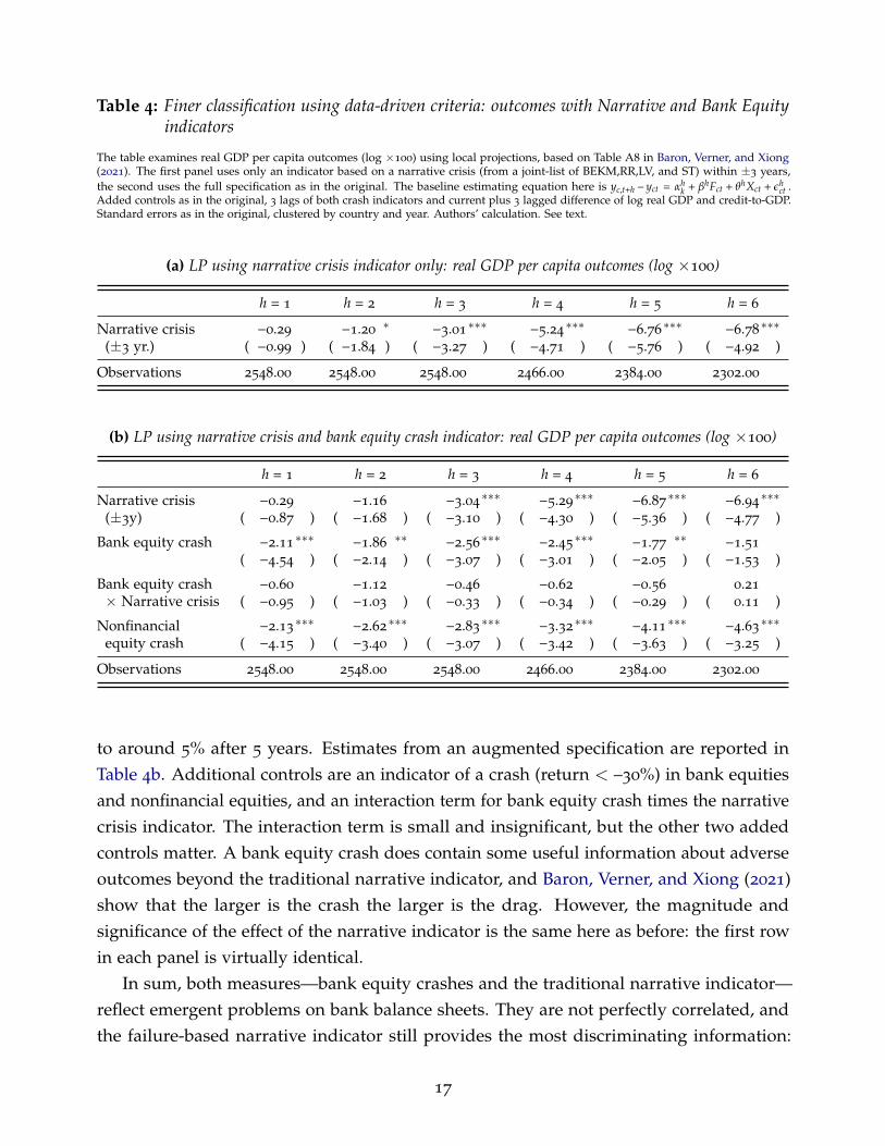
Table 4: Finer classification using data-driven criteria: outcomes with Narrative and Bank Equityindicators

The table examines real GDP per capita outcomes (log ×100) using local projections, based on Table A8 in Baron, Verner, and Xiong(2021). The first panel uses only an indicator based on a narrative crisis (from a joint-list of BEKM,RR,LV, and ST) within ±3 years,the second uses the full specification as in the original. The baseline estimating equation here is yc,t+h – yct = αh

k + βhFct + θhXct + ϵhct .

Added controls as in the original, 3 lags of both crash indicators and current plus 3 lagged difference of log real GDP and credit-to-GDP.Standard errors as in the original, clustered by country and year. Authors’ calculation. See text.

(a) LP using narrative crisis indicator only: real GDP per capita outcomes (log ×100)

h = 1 h = 2 h = 3 h = 4 h = 5 h = 6

Narrative crisis −0.29 −1.20∗ −3.01

∗∗∗ −5.24∗∗∗ −6.76

∗∗∗ −6.78∗∗∗

(±3 yr.) ( −0.99 ) ( −1.84 ) ( −3.27 ) ( −4.71 ) ( −5.76 ) ( −4.92 )

Observations 2548.00 2548.00 2548.00 2466.00 2384.00 2302.00

(b) LP using narrative crisis and bank equity crash indicator: real GDP per capita outcomes (log ×100)

h = 1 h = 2 h = 3 h = 4 h = 5 h = 6

Narrative crisis −0.29 −1.16 −3.04∗∗∗ −5.29

∗∗∗ −6.87∗∗∗ −6.94

∗∗∗

(±3y) ( −0.87 ) ( −1.68 ) ( −3.10 ) ( −4.30 ) ( −5.36 ) ( −4.77 )

Bank equity crash −2.11∗∗∗ −1.86

∗∗ −2.56∗∗∗ −2.45

∗∗∗ −1.77∗∗ −1.51

( −4.54 ) ( −2.14 ) ( −3.07 ) ( −3.01 ) ( −2.05 ) ( −1.53 )

Bank equity crash −0.60 −1.12 −0.46 −0.62 −0.56 0.21

× Narrative crisis ( −0.95 ) ( −1.03 ) ( −0.33 ) ( −0.34 ) ( −0.29 ) ( 0.11 )

Nonfinancial −2.13∗∗∗ −2.62

∗∗∗ −2.83∗∗∗ −3.32

∗∗∗ −4.11∗∗∗ −4.63

∗∗∗

equity crash ( −4.15 ) ( −3.40 ) ( −3.07 ) ( −3.42 ) ( −3.63 ) ( −3.25 )

Observations 2548.00 2548.00 2548.00 2466.00 2384.00 2302.00

to around 5% after 5 years. Estimates from an augmented specification are reported inTable 4b. Additional controls are an indicator of a crash (return < –30%) in bank equitiesand nonfinancial equities, and an interaction term for bank equity crash times the narrativecrisis indicator. The interaction term is small and insignificant, but the other two addedcontrols matter. A bank equity crash does contain some useful information about adverseoutcomes beyond the traditional narrative indicator, and Baron, Verner, and Xiong (2021)show that the larger is the crash the larger is the drag. However, the magnitude andsignificance of the effect of the narrative indicator is the same here as before: the first rowin each panel is virtually identical.

In sum, both measures—bank equity crashes and the traditional narrative indicator—reflect emergent problems on bank balance sheets. They are not perfectly correlated, andthe failure-based narrative indicator still provides the most discriminating information:

17

BVX count 197 narrative failure events, and out of these 193 are called as crises (98%); butout of a count of 269 bank equity crashes, only 138 are called as crises (51%). This showsthat the inclusion of data on bank equity declines complements the narrative approachwith useful auxiliary information.

Summary Finer classifications are feasible and can produce sensible results which comple-ment the binary approach. They can reveal how more intense stress episodes line up withmore adverse outcomes. However, milder episodes may not be associated with significantdrag. These findings remind us that the binary classifications will yield only measures ofaverage effects, and that in reality financial crises come in varying levels of intensity, whichare correlated with key outcomes.

Finer narrative measures can be built but this is a time-intensive, bespoke activity. Thepaucity of widespread, continuous, high-frequency, consistent narrative sources for manycountries or periods is a formidable obstacle. The difficulty of ensuring comparabilityacross sources with varying textual content to allow the datasets to be pooled for large-scalepanel analysis may also keep the traditional binary indicator in business.

Finer data-based measures present different tradeoffs. Data availability is broader andeasier, at least where financial data are already compiled. Comparability across historicalepisodes is better ensured by a hard definition grounded in observable market data. Yet it isclear that even this measure can’t capture everything related to a crisis and fully substitutefor the narrative information on failures in the traditional binary indicator.

As a final note, it is worth noting that almost all measures of financial crises point to theconclusion that financial crises are associated with a sharp decline in real economic activity.It is unlikely that such a finding is the result of look-back biases or subjective evaluation ofwhat constitutes a crisis. The severe economic downturns associated with financial criseswarrants a further consideration of their causes. The next section turns to this question.

3. Financial crisis predictability and causality

Financial crises are associated with severe and protracted downturns in economic activity.So it is no surprise that a large body of research is dedicated to the question of the sources offinancial crises. For the sake of argument, it is useful to separate views on this question intotwo extremes. Are financial crises random events that strike an otherwise stable economy?Or, in contrast, is there a set of factors that systematically predict financial crises? Thissection shows that the evidence strongly favors the second view: financial crises are indeedpredictable which raises challenging questions for the theory of business cycles.

18

3.1. Credit expansion and asset price growth

Pre–Global Financial Crisis research The idea that asset price growth and credit expan-sion are crucial to the prediction of financial crises is an old one in economics, showing upprominently in the work of Kindleberger (1978) and Minsky (1986). The modern approachof using large data sets and econometric tools to detect predictability began in the aftermathof the banking crises of the 1980s and 1990s. This initial wave of research focused mostlyon data sets covering the 1970s through 2000.

Illustrative of this literature is Borio and Lowe (2002) who focus on a sample of 34

countries from 1970 to 1999. They conclude that “sustained rapid credit growth combinedwith large increases in asset prices appears to increase the probability of an episode offinancial stability.” The statistical analysis in the study compares the statistical power ofasset prices, credit growth, and investment growth in predicting financial crises usingthe Bordo, Eichengreen, Klingebiel, and Martınez-Perıa (2001) crisis classification. Thesefindings follow upon the influential work by Kaminsky and Reinhart (1999), who conditionon financial crises and show that rapid credit growth is a salient feature of the pre-crisisperiod. Kaminsky and Reinhart (1999) point to the importance of financial liberalization inexplaining the rapid credit growth, a factor explored in more detail in subsection 3.2.

Other notable contributions among this first wave of research on the predictability offinancial crises are Caprio and Klingebiel (1996), Demirguc-Kunt and Detragiache (1998),Glick and Hutchison (2001), Hutchison and McDill (1999), Hardy and Pazarbasioglu (1999),Gourinchas, Valdes, and Landerretche (2001), and Eichengreen and Arteta (2002), amongothers. Table 5 contains a brief overview of all of these articles, listing the number ofcountries covered, the sample years, whether the study includes emerging markets, anda brief summary of the factors that the study finds help statistically predict crises. A risein private credit, measured either using private credit growth or the change in the privatecredit to GDP ratio, emerges as a central factor in many of these studies. Asset pricecorrections, following a period of elevated valuations, also often appear as a theme.

However, this earlier wave of research emphasizes open economy issues to a largerdegree than in the later literature written after the Global Financial Crisis.7 This is in partdue to a focus on crisis countries in the 1980s and 1990s that were small open-economyadvanced economies, or Latin American and East Asian emerging economies. Openeconomy issues were naturally a greater focus of this literature, given the important rolethat factors like cross-border capital flows and real exchange rate movement played in therun-up to crises in these countries, and also in the subsequent adjustment process, aspects

7Although, as shown below, open economy issues do play an important role in evaluation of the GlobalFinancial Crisis.

19

Table 5: Literature Review

# Authors No. of Sample EME Significant(Year) countries years predictors

1 Caprio and Klinge-biel (1996)

29 studied in-depth(69 discussed over-all).

Country-specific in-stances identi-fied, earliest in1977 for Spain.

✓ - Macro: Volatility in terms of trade; Highinflation; Large interest rate spread.- Regulatory and accounting frameworks:Poor incentives for reporting losses; Lowbank capitalization levels; Political suasionover underwriting decisions.

2 Demirguc-Kuntand Detragiache(1998)

Max. 65 and min.45 from IMF’s IFSdatabase.

1980–94 ✓ - Banking sector: Capital outflows; Highprivate-sector share of credit; Explicit depositinsurance scheme.- Macro: Low GDP growth; High real in-terest rates; High inflation; Terms of tradedeterioration

3 Glick and Hutchi-son (2001)

Unbalanced panelof 90 countries.

1975–97 ✓ - Currency crisis: Greater real exchange rateovervaluation; Higher ratio of M2/foreignreserves; Lower export growth; Lagged bank-ing crisis.- Banking crisis: Decline in GDP growth;Greater liberalization

4 Hutchison andMcDill (1999)

44 OECD indus-trial countries, withprimary focus onJapan.

1975–97 ✗ - Macro: Sharp fall in asset prices; Decline inreal GDP growth; Real credit growth- Institutional: Lower central bank indepen-dence; Increased explicit deposit insurance;Greater financial liberalization

5 Kaminsky andReinhart (1999)

5 industrial and15 developing coun-tries.

Country-specific, broadly1970s to 1995.

✓ - Currency crisis: Lagged banking crisis (pre-dicts and aggravates); Contagion in capitaloutflow.- Banking crisis: Lagged currency crisis (ag-gravates, does not predict).- Common factors (Twin crisis): Lax fi-nancial supervision; Growth in credit/GDP;Growth in M2/foreign reserves; sharp de-cline in asset prices; Falling exports; De-terioration in terms of trade; Higher fiscaldeficit/GDP.

6 Hardy andPazarbasioglu(1999)

50 countries, with38 experiencing cri-sis and 12 acting ascontrols.

1980–96 ✓ - Real sector: Fall in real GDP growth; Pri-vate consumption boom.- Banking sector: Fall in deposit liabili-ties/GDP ratio; Boom-bust in private-sectorcredit/GDP; Boom-bust in the ratio of grossforeign liabilities of the banking system toGDP .- Other factors: Boom-bust in inflation; Risein real interest rate; Appreciation in real ef-fective exchange rate; Fall in real growth inimports.

7 Gourinchas, Valdes,and Landerretche(2001)

91 developingand developedcountries.

1960–96 ✓ - Domestic macro factors: Rise in privatecredit/GDP; Decline in potential (trend)GDP; Boom-bust in investment; Rising do-mestic real interest rate.- Domestic policy factors: Worsening of gov-ernment deficit to GDP ratio; Decline in for-eign reserves.- International factors: Boom-bust in currentaccount; Appreciation in real exchange rate;Boom-bust in private capital inflows; Risingshort-term debt.- External factors: Boom-bust in terms oftrade.

continued . . .

20

. . . continued# Authors No. of Sample EME Significant

(Year) countries years predictors

8 Eichengreen andArteta (2002)

75 developingcountries, basedon Caprio &Klingebiel (1999).

1975–97 ✓ High rate of domestic credit growth; Lowreserves/M2 ratio; Rise in interest rates andfall in real GDP in advanced economies causecrisis in EMEs, but only in pre-1990s crisis;Financial liberalization

9 Borio and Lowe(2002)

34 countries, basedon criteria detailedon page 12.

1970–99 ✓ Boom-bust in asset price inflation.

10 Schularick and Tay-lor (2012)

14 developed coun-tries.

1870–2008 ✗ Past 5-year boom in bank credit growth;Higher financialization (higher credit/GDPor increased size of stock markets); Highleverage and low capital/liquidity buffers.

11 Jorda, Schularick,and Taylor (2015b)

17 1870–2013 ✗ Leveraged bubbles (interaction of asset pricebubbles and credit booms), only housingbubbles (not equity bubbles) are significant.

12 Richter, Schularick,and Wachtel (2021)

17 1870–2016 ✗ Credit growth; Higher capital-to-asset andloan-to-deposit ratios predict crisis.Asset prices: Only housing bubbles (not eq-uity bubbles) are significant.

13 Greenwood, Han-son, Shleifer, andSørensen (2020)

42 1950–2016 ✓ Credit expansion and asset price booms(red zone): Nonfinancial business creditgrowth and stock market valuations haverisen sharply; Household credit growth andhome prices have risen sharply.

noted long ago by Dıaz-Alejandro (1985) and re-emphaszied by McKinnon and Pill (1996).

We highlight three factors that emerged as central to the prediction of crises in suchsmall-open economy cases: inflation, the terms of trade, and the real exchange rate.Kaminsky and Reinhart (1999) show the dynamics of both the real exchange rate and theterms of trade in the years around a banking crisis. Both show a similar pattern: the realexchange rate appreciates and terms of trade improve in the years prior to the crisis, butthe crisis is associated with a rapid deterioration in both. This boom-bust pattern in realexchange rates and the terms of trade is a robust pattern shown in this earlier wave ofresearch (e.g., Caprio and Klingebiel, 1996; Hardy and Pazarbasioglu, 1999; Gourinchas,Valdes, and Landerretche, 2001).

Post–Global Financial Crisis research The Global Financial Crisis of 2008 led to a newwave of research focused on the factors that predict financial crises. Overall, this bodyof research focuses more on advanced economies, and it has the advantage of data setscovering a much longer time period. Credit growth and asset price growth emerge as evenstronger predictors once a longer time series is used for estimation.

Schularick and Taylor (2012) and Jorda, Schularick, and Taylor (2015b) introduce a novellong-run data base covering key macroeconomic variables for 17 advanced economies from1870 onward (see also Jorda, Schularick, and Taylor, 2017). The key measure of private

21

credit is bank loans to domestic households and non-financial corporations. Using this dataset, Schularick and Taylor (2012) focuses on predictability, using a specification where theprobability of a financial crisis event is related to lagged real private credit growth. Theyfind robust statistical power of credit growth in predicting a financial crisis using ROC(receiver operating characteristic) criteria, an aggregate of Type 1 and Type 2 errors. Theresults hold in the pre- and post-WW2 subsamples, and with a battery of controls.

Later work confirms these findings with variant definitions of the credit boom variable,and to summarize these findings, a simple logit specification in this vein would be

logit (pct) ≡ log(

pct1 – pct

)= α + β∆5CREDGDPct + γXct + ϵct ,

where the probability pct ≡ P(Crisisct = 1) and the dependent variable is the log odds ratioof a financial crisis is estimated as a function of the 5-year lagged change in private creditto GDP, denoted ∆5CREDGDP, and controls X, which would be estimated on annual datafor the 17 countries since 1870.

Illustrative results showing the predictive margins within a roughly mean plus/minus2 s.d. range of the credit variable are shown in Figure 6a, with no controls. The uncon-ditional probability of a crisis is 2.5% (1 in 40 years), corresponding to the mean value of∆5CREDGDP. However, when the credit growth variable rises one s.d. above its mean, theexpected crisis probability almost doubles to 5% (1 in 20 years), and at two s.d. above themean the expected crisis probability is near 10% (1 in 10 years), four times its baseline level.

Illustrative results for the prediction of the type of recession peak, financial versusnormal, produce similar results, as shown in Figure 6b. Now the outcome variable isan indicator equal to one when the peak is a financial crisis peak, rather than a normalpeak, using the Jorda, Schularick, and Taylor (2013) peak classification. The unconditionalprobability of a peak being a financial crisis peak is about 0.2 but the probability is againincreasing in lagged credit growth.

The main results in Schularick and Taylor (2012) use full in-sample information, but inan out-of-sample exercise they show that estimates of the model up to the 1980s would haveyielded significant predictive success in subsequent years. Richter, Schularick, and Wachtel(2021) focus on a similar data set. They define credit booms as situations where log realprivate credit per capita rises by more than a standard deviation relative to the predictedtrend using only past information. Consistent with Schularick and Taylor (2012), they findstrong predictive power of credit booms out of sample. Jorda, Schularick, and Taylor (2016)distinguish the explanatory power of mortgage and non-mortgage credit. In the full sample,both mortgage credit and non-mortgage credit predict financial crises, with non-mortgage

22

Figure 6: Credit booms and elevated asset prices predict a financial crisis

The figure shows logit predictive margins for financial crisis events, using lagged information, where the estimating equation takes theform logit (pct) = α + β∆5CREDGDPct + γXct + ϵct . and the sample mean (µ) ± 2 s.d (σ) range of the CREDGDP variable is shown. Inthese estimates there are no added controls. In the left panel, the data are all country-year ct observations and the outcome variable is afinancial crisis using the JST classification in the advanced economy long panel. In the next two panels, the data are all country-year ctobservations that correspond to cyclical peaks and the outcome variable is a financial crisis peak using the JST classification. The lastpanel includes an asset price bubble indicator. Authors’ calculation. See text.

(a) Baseline logit,credit growth only,predicting crisis years

μ±σμ=5.08σ=12.38

0.0

2.0

4.0

6.0

8.1

Prob

abili

ty o

f a fi

nanc

ial c

risi

s pe

ak(u

ncon

ditio

nal)

-20 -10 0 10 20 305-year change in credit/GDP

(b) Baseline logit,credit growth only,predicting crisis recession peaks

μ=4.31σ=13.36

μ±σ

0.1

.2.3

.4.5

Prob

abili

ty o

f a fi

nanc

ial c

risi

s pe

ak(c

ondi

tiona

l, as

soci

ated

with

a c

yclic

al p

eak)

-20 -10 0 10 20 305-year change in credit/GDP

(c) Expanded logit,credit growth and asset prices,predicting crisis recession peaks

μ=4.31σ=13.36

μ±σ

0.1

.2.3

.4.5

Prob

abili

ty o

f a fi

nanc

ial c

risi

s pe

ak(c

ondi

tiona

l, as

soci

ated

with

a c

yclic

al p

eak)

-20 -10 0 10 20 305-year change in credit/GDP

No asset price bubbleAsset price bubble

credit displaying stronger statistical power in pre-World War 2 sample. However, sinceWorld War 2, the strength of mortgage credit as a predictor has grown considerably.

To confront the issue of whether asset price booms also contribute meaningfully toelevated financial crisis risk, Jorda, Schularick, and Taylor (2015b) collate further data serieson equity and housing prices for the long-panel of advanced economies. They develop a“bubble indicator” based on whether the asset price in a given year is more than one s.d.above its de-trended value (using a lowpass filter) and whether there is also a subsequentlarge correction. An illustration of this approach is in Figure 6c, where the sample is againrestricted to recession peaks, and the logit estimation is augmented to include a bubbleindicator for either asset price. When there is no bubble in either asset price, crisis risk isgenerally low. In contrast, when there is either kind of bubble, crisis risk is significantlyelevated, by a factor of roughly 1.5 in the mid-range of credit growth.8

8The study by Richter, Schularick, and Wachtel (2021) takes a different approach but comes to a similarconclusion. After demonstrating the strong predictive power of credit expansion on the probability of afinancial crisis, this article splits credit booms by whether they end in a financial crisis or not. It then comparesthe characteristics of the booms that do and do not end in a crisis. House price growth emerges as a centralfactor. In fact, the statistical power of the difference in house prices for booms and do and do not end in abust is larger than for any other variable. House prices are closely linked to mortgage debt and constructionbooms, which helps connect this finding to the broader evidence that household and mortgage debt are themost powerful predictors of financial crises. For early studies recognizing the importance of house prices inexplaining financial crises, see Reinhart and Rogoff (2008, 2009a).

23

This idea is taken further in a post-WW2 short-panel setting, which includes emergingeconomies, in an analysis by Greenwood, Hanson, Shleifer, and Sørensen (2020). Theirsample includes 42 countries from 1950 to 2016, and they use the Baron, Verner, and Xiong(2021) financial crisis indicator as their outcome variable. Their data set also includes houseprice and business equity price growth, along with measures of both household and non-financial firm debt. Credit growth still predicts financial crises. However, asset price growthhelps boost the predictive power, leading the authors to construct an indicator they callthe “Red Zone” — denoting a country that finds itself in the top third of both the historicalcredit growth and asset price growth distribution, a particularly strong predictor of whethera financial crisis occurs within the next three years. The study demonstrates substantialout-of-sample predictive power of the Red Zone indicator variable on a subsequent crisis.

3.2. What causes the credit expansion?

Financial crises are systematically preceded by a large rise in the quantity of credit and adecline in its cost. As a result, exploring the causes of a financial crisis means exploring thereasons for the credit expansion that precedes it, with a focus on the supply side of credit.

One factor often cited as an important cause of credit expansion is financial liberalization,especially in an open economy setting. This theme emerges prominently in research writtenin the aftermath of the banking crises of the 1980s and 1990s, which were frequentlypreceded by deregulation of the financial sector. Demirguc-Kunt and Detragiache (1998)presents one of the earliest attempts to systematically measure financial liberalization acrossmany countries over time. Their review of policy changes leads them to conclude that ”thea removal of interest rate controls was the centerpiece of the liberalization process.” Theyshow that such liberalization often precedes the banking crises of the 1980s and 1990s.9

The argument that financial liberalization is an important driver of credit boom is putforth in Kindleberger and Aliber (2005), who write that “a particular recent form of dis-placement that shocks the system has been financial liberalization or deregulation in Japan,the Scandinavian countries, some of the Asian countries, Mexico, and Russia. Deregulationhas led to monetary expansion, foreign borrowing, and speculative investment.” A largebody of research focused on the Latin American experience in the 1970s and 1980s, and theScandinavian experience of the 1980s and 1990s, emphasizes the importance of financialliberalization in explaining the boom-bust cycle in credit and the real economy.10

9Several articles follow the Demirguc-Kunt and Detragiache (1998) argument that the removal of interestrate controls was a central piece of financial liberalization . These include Glick and Hutchison (2001) andKaminsky and Reinhart (1999), among others. These studies consistently find that financial liberalizationprecedes banking crises.

10See Mian and Sufi (2018) for a summary of this literature. Key citations for Latin American include

24

Figure 7: The response of credit to financial liberalization and monetary policy shocks

The figure shows local projections of the deviation of the path of credit-to-GDP after a shock using the JST outcome measure in theadvanced economy long panel. In the left panel, the shock is a change in the degree of financial liberalization using the dataset ofKaminsky and Schmukler (2008) for the period 1973–2005 In the right panel, the shock is a change in monetary policy proxied by theshort-term local interest rate, identified using the Jorda, Schularick, and Taylor (2015a) trilemma instrument for the full sample since1870. The latter also includes responses for both the mortgage and non-mortgage components of credit. Authors’ calculation. See text.Authors’ calculation. See text.

(a) Financial liberalization shock

0.0

1.0

2.0

3.0

4D

evia

tion

of c

redi

t/G

DP

from

bas

elin

e

0 1 2 3 4 5Years after shock

1 s.d financial liberalization shock

(b) Monetary policy shock

0.0

1.0

2.0

3.0

4D

evia

tion

of c

redi

t/G

DP

from

bas

elin

e

0 1 2 3 4 5Years after shock

1 s.d. trilemma loosening shock — mortgage credit only — nonmortgage credit only

Some illustrative evidence is shown in Figure 7a using local projections. The outcomevariable is private credit to GDP, denoted CREDGDPct, from the Jorda, Schularick, andTaylor (2017) bank loan measure, and the sample is the long-panel of advanced economies.The shock is a change in the degree of financial liberalization, treated as exogenous,according to a set of indices constructed by Kaminsky and Schmukler (2008) for theperiod 1973–2005, a range of dates which closely encompasses the great era of financialliberalization in both advanced and emerging economies. The index used here is thestandardized sum of three measures of the domestic financial sector, the stock market,and the capital account. The figure clearly shows that in the 5 years after a financialliberalization event, changes in credit to GDP, which were on a positive long-run postwartrend anyway, had a tendency to accelerate even more rapidly.

Financial liberalization is one driver of credit expansions. And it may provide usefulexogenous variation in some episodes. However, the fact that liberalizations are lowfrequency, occur in waves and in many countries at roughly the same time, casts doubton the view that liberalization is the only or even the main primitive underlying shockthat leads to the repeated credit booms of interest occurring at high-frequency throughout

Dıaz-Alejandro (1985), and key citations for Scandinavia are Englund (1999) and Jonung and Hagberg (2005).

25

history. Furthermore, it is not obvious that financial liberalization in the absence of changesin credit supply should be associated with lower interest rates and a rise in asset prices (e.g.,Justiniano, Primiceri, and Tambalotti, 2019). Instead, it is quite likely that liberalization, byopening a gate, enables other fundamental economic forces in the local or global economyto play out, creating the possibility of new or more elastic financial flows (intermediateclaims, or leverage) relative to existing investment opportunities (real assets, actual orpotential).

What are these broader forces driving flows of credit? One recent manifestation is theidea of a “global saving glut” proposed by Bernanke (2005) to explain the large capitalinflows into many advanced economies from 1998 to 2006. An older version of this ideafrom the 1970s was the ”petro-dollar” recycling argument that a rise in oil prices createdan excess of dollar deposits in advanced economy banks, which were subsequently loanedto Latin American governments and corporations (e.g. Pettis, 2017; Devlin, 1989; Folkerts-Landau, 1985). In both of these narratives, some global change in savings leads to a largeaccumulation of deployable financial capital, which enters into certain liberalized countriesand potentially drives a boom and bust cycle in credit.

A related idea has emerged recently with the rise in income inequality. There is plentifulevidence that the rich have a higher propensity to save out of lifetime income, thereforecreating a “saving glut of the rich” when top income shares rise. Kumhof, Ranciere, andWinant (2015) motivate their model with the observation that both the Great Depressionand the Great Recession in the United States were preceded by a rise in income inequalityand more borrowing by lower- and middle-income households.11 Mian, Straub, and Sufi(2020b) focus on the United States from 1963 to 2016 and show that the rise in top incomeshares since the 1980s has been associated with a saving glut of the rich. Furthermore, thissaving glut of the rich has financed a large rise in household and government debt.

In line with this evidence, Mian, Straub, and Sufi (2020a) build a model that incorporatesthe empirically-supported idea that the rich have a higher propensity to save out of lifetimeincome, so that a rise in the income share of the rich, in equilibrium, leads to a rise inborrowing by the non-rich. Such a buildup of debt eventually lowers aggregate demand inthe future as low saving propensity individuals (the non-rich) make debt service paymentsto high saving propensity individuals (the rich). Going further, Klein and Pettis (2020) linkthe saving glut of the rich to the global saving glut by suggesting that rising current accountsurpluses in Germany and China since the 1980s have been due to the rise in inequalitywithin those countries.

Of a more cyclical and high frequency nature, monetary policy may play an important

11See Eichengreen and Mitchener (2003) for a discussion of the U.S. credit boom of the 1920s.

26

role in explaining bursts of credit expansion, as lower interest rates may encourage banksto expand credit supply and/or take more risk. Jorda, Schularick, and Taylor (2015a) utilizean identification strategy based on the fact that countries with a fixed exchange rate regimeexperience fluctuations in short-term interest rates that are largely independent of localeconomic circumstances, a consequence of the trilemma of international macroeconomics.Using this empirical strategy with a data set covering 17 advanced economies over the past140 years, they show that a loosening shock to local interest rates fuels an expansion inlending against real estate and growth in house prices. These are the conditions whichheighten the risk of a financial crisis. Illustrative evidence is shown in Figure 7b using localprojections, where the shock is a trilemma-identified 1 s.d. decline in local interest rates,and a significant credit growth response is seen, especially for mortgage credit.

Monetary policy by the U.S. Federal Reserve is shown to be a particularly importantfactor in explaining the global financial cycle according to Miranda-Agrippino and Rey(2020). Using a data set that begins in 1980, this study demonstrates that a single globalfactor explains a substantial amount of the variation in the price of risky financial assetsaround the world. Furthermore, this global factor reacts to changes in U.S. monetarypolicy, with a contraction in U.S. monetary policy leading to a tightening of global financialconditions. While Miranda-Agrippino and Rey (2020) do not focus specifically on thequestion of financial crises, it is likely that the patterns they uncover are related to theglobal boom and bust episodes seen over the past 40 years.

3.3. Behavioral biases, incentives, and predictability

The credit booms that predict financial crises are associated with a low cost of debt,and a low cost of risky debt in particular. An early study on such predictability byGreenwood and Hanson (2013) focuses on the United States and shows that a narrowing ofcredit spreads between high yield and investment grade corporations together with highissuance by low credit quality firms relative to high credit quality firms forecasts low excessreturns to corporate bondholders. Lopez-Salido, Stein, and Zakrajsek (2017) build on thisempirical finding to show that these same measures of heightened credit market sentimentpredict a reversal in credit market conditions and subsequently lower real GDP growth.Krishnamurthy and Muir (2017) collect novel data covering the interest spread betweenhigher and lower grade bonds for 19 countries data going back 150 years. They confirm therelationship in the literature that crises are preceded by unusually high credit growth. Theyalso show that crises are preceded by unusually low and falling credit spreads betweenhigher and lower grade bonds. In other words, riskier firms are able to finance themselvesat a relatively lower cost during the credit booms that precede financial crises.

27

These findings on spreads fit into the broader picture. It should be clear that a lowspread between more risky and less risky debt is closely related to the idea that risky assetprices are high prior to financial crises. Holding expected cash flows fixed, a low interestspread between risky and less risky bonds would imply a relatively high risky asset price.

These complementary results in a large and growing body of work are importantbecause they help narrow the set of theories that can plausibly explain why credit boomspredict financial crises. Credit booms are periods in which the cost of financing risky debtis low and risky asset prices are bid up. The low cost of debt financing in combination withthe rapid growth in debt is why many refer to these episodes as a “credit supply expansion,”a “credit boom,” or “frothy credit-market conditions.” Creditors appear to become morewilling to extend credit at a lower cost during the booms that precede financial crises.

The theoretical literature has advanced two broad paths to explain these results. Inthe first broad path, there are rational expectations models in which a financial crisis isparticularly painful in the aftermath of credit expansion given incentive and informationfrictions that build up during the boom part of the boom-bust cycle. The second broad pathargues that deviations from rational expectations are a crucial element in explaining thecredit boom-crisis nexus.

The first class of models includes the studies by Gary Gorton and coauthors (e.g, Gortonand Ordonez (2014, 2019); Dang, Gorton, Holmstrom, and Ordonez (2017); Dang, Gorton,and Holmstrom (2020)). The central idea in this research agenda is that the short-termdebt securities that often fuel a credit boom and are at the heart of explaining the crisisare optimally structured to be ”information-insensitive.” Investors choose not to informthemselves on the quality of the underlying collateral, which can help fuel economic activityin the absence of any negative shock.

During the credit boom, the lack of information production leads to a depreciationof information about the quality of collateral backing the debt instruments. In such anenvironment, if there is an aggregate shock that reduces the value of the underlyingcollateral, there can be a ”loss of confidence” in the collateral which triggers a panic. Akey point of the framework is that a small shock can cause big problems if the underlyinginformation on collateral value has deteriorated significantly during the credit boom. Gortonand Ordonez (2019) argue that credit booms in which productivity falls substantially duringthe boom will be especially vulnerable to a small amount of negative information beingsuddenly revealed.

Diamond, Hu, and Rajan (2020) build a model in which frictions related to cash flowpledgeability lead creditors to rationally lend large amounts when there is a high probabilityof a high liquidity state in the future. They do so knowing that the realization of a low

28

liquidity state in the future will be painful, as the amounts of debt taken on by expertmanagers of firms leads firms to be sold to less productive outsiders. The incentive to shiftrisk by financial intermediaries lies at the heart of models by both Acharya and Viswanathan(2011) and Coimbra and Rey (2017). Both models predict that financial fragility will riseduring a credit boom, amplifying a decline in economic activity conditional on a negativeshock.

While incentive and information frictions can amplify the negative effects of a boomfollowed by a negative shock, these frictions do not generate systematic predictive power ofcredit booms on asset prices, in particular. Such predictability brings behavioral biases tothe forefront when considering the boom-bust cycle associated with financial crises.

A particularly convincing study showing that flawed expectations are an importantdriver of credit expansions is the analysis of bank equity returns by Baron and Xiong (2017).This study builds on the evidence described above that a rise in the bank credit to GDPratio predicts lower subsequent growth and a heightened probability of financial crises.The authors construct bank equity returns for 20 developed economies from 1920 to 2012.This allows for a detailed analysis of the returns realized to the holders of bank equityafter an expansion in credit. They show that a rise in the bank credit to GDP ratio overthe past three years that is above the 95th percentile of the historical distribution predictsan average return on bank equity over the next three years of –37.3%. Such a bank creditexpansion predicts a heightened probability of a crash in bank equity prices, and yet bankcredit expansion also predicts lower future returns. The ability of bank credit expansionknown in year t to predict a large negative subsequent return on bank equity prices fromyears t to t + 3 is difficult to reconcile with a framework built on rational expectations ofbank equity holders.

Illustrative evidence on trends around financial crises are shown in Figure 8 for theJST long panel. Using an event-study approach, the average evolution of each variable isplotted relative to the peak year of the cycle. Averages are displayed separately for normalrecessions (solid blue line) and financial crisis recessions (dashed red line). The first row offour charts shows the familiar timing of events and macro aggregates. Crisis probability isof course high in the ±2 year window around a financial crisis recession, by construction,given the JST peak classification; it is negligible in normal recessions, although it is notexactly zero except in year zero, since nearby financial crisis events may be associated witha different nearby cyclical peak in JST. Real GDP per capita growth decelerates after arecession peak, but much more so in a financial crisis recession as expected. Likewise, arecession is associated with the onset of a disinflationary period of several years, but thetrend is much more pronounced in a financial crisis recession. Finally, the fourth chart

29

Figure 8: Key macro-financial trends in normal and financial crisis recessions from an event-study

The figure shows macro-financial trends in normal and financial crisis recessions. The time axis is normalized to make year 0 coincidewith the cyclical peak. The recessions classification follows Jorda, Schularick, and Taylor (2013), and updates thereto. All variables arefrom the JST Macrohistory dataset, except bank equity returns from Baron and Xiong (2017), credit spreads from Krishnamurthy andMuir (2017) and capital and loan/deposit ratios from Jorda, Richter, Schularick, and Taylor (2021). Growth rates, inflation, and totalreturns are expressed in log ×100 units. Credit/GDP is expressed in percentage points. Credit spreads are normalized and expressed inpercentage deviation from the country mean. Authors’ calculation. See text.

(a) Crisis probability

-10

010

2030

4050

Perc

ent

-5 -4 -3 -2 -1 0 1 2 3 4 5Year relative to peak

NormalFinancial crisis

(b) GDP p.c. growth

-3-2

-10

12

34

Perc

ent

-5 -4 -3 -2 -1 0 1 2 3 4 5Year relative to peak

NormalFinancial crisis

(c) Inflation

-10

12

34

5Pe

rcen

t

-5 -4 -3 -2 -1 0 1 2 3 4 5Year relative to peak

NormalFinancial crisis

(d) Change in credit/GDP

-2-1

01

23

45

Perc

ent

-5 -4 -3 -2 -1 0 1 2 3 4 5Year relative to peak

NormalFinancial crisis

(e) Credit spreads

-50

050

100

150

Perc

ent

-5 -4 -3 -2 -1 0 1 2 3 4 5Year relative to peak

NormalFinancial crisis

(f) Bank equity total return

-60

-40

-20

020

4060

Perc

ent

-5 -4 -3 -2 -1 0 1 2 3 4 5Year relative to peak

NormalFinancial crisis

(g) Real stock price growth

-20

-10

010

20Pe

rcen

t

-5 -4 -3 -2 -1 0 1 2 3 4 5Year relative to peak

NormalFinancial crisis

(h) Real house price growth

-6-4

-20

24

68

Perc

ent

-5 -4 -3 -2 -1 0 1 2 3 4 5Year relative to peak

NormalFinancial crisis

(i) Bank capital ratio

6.5

77.

58

8.5

99.

510

Perc

ent

-5 -4 -3 -2 -1 0 1 2 3 4 5Year relative to peak

NormalFinancial crisis

(j) Bank loan/deposit ratio

8590

9510

010

511

011

5Pe

rcen

t

-5 -4 -3 -2 -1 0 1 2 3 4 5Year relative to peak

NormalFinancial crisis

30

shows that financial crisis recession peaks are preceded by credit booms and followed bycredit crunches much more so than normal recessions.

The second row of charts in Figure 8 shows some interesting financial market covariatesusing selected asset prices. The first chart shows the Krishnamurthy and Muir (2017)normalized credit spread, which is the percent difference of the credit spread from itscountry mean (so 0% means the spread is equal to this average), and clearly spreads aretighter than average (50% lower) before a financial crisis recession peak, and much widerimmediately after (50%–100% higher), compared to the minimal variation seen in normalrecession events. The next chart shows the Baron and Xiong (2017) real total return on bankequities, which is a little high before a normal recession peak and indistinguishable fromzero after; but near a financial crisis recession peak, bank equities experience a very largerun up before, and a large crash afterwards, with significant negative real returns (note thatthese are log×100 units). Finally, we can see that distress clearly spills over into broaderaggregate asset prices, where the onset of a financial crisis recession event similarly impliesmuch larger and predictable reversals for investors exposed to the stock market or housingmarket, as shown in the last two charts.

The recent study by Richter and Zimmermann (2019) looks into the dynamics that occurat banks to uncover the specific biases that may help explain these results. In particular, thestudy points to the extrapolation of a sudden rise in bank profits as the origin of the bankcredit expansion. A rise in profits predicts a rise in lending, and, ultimately, financial crisescan emerge when profits further into the future eventually fall. Delving further into therise in profits, the study finds that a key reason for the rise in the profits is a decline in loanloss provisions. All of these patterns are consistent with the idea that a reason behind theexpansion of credit is the rise in optimism by bank managers that comes after the realizationof high profits on lending. This rise in optimism can explain why the quantity of creditexpands, why interest rates fall, and why bank equity profits are predictably negative oncethe credit expansion has become sufficiently large. In a related finding, Mian, Sufi, andVerner (2017) show that the decline in the mortgage interest rate relative to the sovereignbond interest rate is a powerful predictor of a rise in the household debt to GDP ratio.

Further insight into actors’ motivations emerges from recent work on bank capital andits consequences by Jorda, Richter, Schularick, and Taylor (2021). They collect new data forthe long panel of advanced economies on the liability side of the banking system, trackingthe evolution over time of bank capital ratios, and well as other key ratios for the fundingmix, such as loan to deposit ratios and the fraction of non-core funding. The standardassumption about governance, which has guided recent regulatory activity, is that if bankshave more “skin in the game” they should engage in more prudent risk-management

31

behavior and thereby reduce the probability that financial institutions will face large lossesthat put their existence at risk. However, the historical evidence goes against this argument.Banks have failed consistently across time, in times of high capital ratios like the late 1800s,and in times of low capital ratios like the last 30–40 years. Crisis prediction regressionsshow no association, or possibly an inverted one, between capital ratios and crisis risk.Jorda, Richter, Schularick, and Taylor (2021) also develop an instrument for changes in bankcapital, giving their results a causal interpretation: higher bank capital ratios do not reducethe risk of crises. Thus, consistent with Baron and Xiong (2017), bank managers and ownersseem unaware risks are rising, and capital levels seem to make no difference as one mightassume if the incentives of rational agents were well aligned. In contrast, other balancesheet ratios such as the loan to deposit (LtD) ratio appear to have significant predictivepower, and this remains even after controlling for lagged credit growth. Illustrative patternsfor the capital and LtD ratios are shown in the third and final row of charts in Figure 8.

Systematic extrapolation errors may not be just confined to actors in the financial sector,such as lenders and borrowers. The expansion of credit is also associated with systematicforecast errors of GDP growth by leading world organizations such as the OECD andthe IMF. This result is demonstrated in Mian, Sufi, and Verner (2017), who show that theexpansion of the household debt to GDP ratio from year t – 4 to year t – 1 can systematicallypredict GDP growth forecast errors from year t to year t + 3. The forecasts are made in yeart, which implies that a factor known for sure at time t predicts forecast errors going forward.Forecasters appear to systematically miss the power of credit expansion in predicting lowersubsequent growth.

All told, the emerging historical evidence supports the existence of systematic behavioralbiases in explaining credit cycles, and such evidence has spurred a rise in theoreticalresearch trying to model the evolution of beliefs in a framework departing from rationalexpectations (e.g., Bordalo, Gennaioli, and Shleifer, 2018; Greenwood, Hanson, and Jin,2016; Krishnamurthy and Li, 2020; Maxted, 2020).

3.4. Triggers

Financial crises are predictable at the 3 to 5 year horizon, but that should not be seen asdecreasing the importance of understanding the specific immediate factors that trigger thecrisis itself. The seminal work by Diamond and Dybvig (1983) points to the importanceof multiple equilibria with demandable debt financing, and the bank run equilibrium inthis model is undoubtedly a powerful explanation for the events that triggered the GlobalFinancial Crisis in 2008.

In terms of the specific factors that tip the scale from boom to bust, a rise in debt service

32

payments is a likely culprit. Drehmann and Juselius (2014) and Drehmann, Juselius, andKorinek (2018) utilize a data set covering new borrowing and debt service flows for apanel of 16 countries from 1980 to 2015. They focus in particular on the debt service ratio(DSR), which represents the interest and principal payments made by borrowers scaled bydisposable personal income. Like other researchers, they find that a rise in private credit isa strong predictor of a financial crisis. However, they also show that a rise in the DSR is ashort-run factor that may explain how the crisis is actually triggered.

The dynamics they illustrate suggest that an innovation to new borrowing leads toa slow but steady rise in the DSR. By three to five years after the initial innovation, theDSR begins to rise substantially. A banking crisis becomes much more likely as these debtservice payments peak. As Drehmann and Juselius (2014) write, ”the DSR’s [debt-serviceratio] early warning properties are especially strong in the two years immediately precedingcrisis. In the last four quarters before crises, the DSR is even a nearly perfect indicator.”

It is well established that economic downturns often begin with banking sector distress,a tightening of credit conditions, and a widening of credit risk spreads (e.g., Lown andMorgan, 2006; Gilchrist and Zakrajsek, 2012). A recent literature focuses on higher frequencymeasures that predict a decline in economic growth at the one-year or less horizon (e.g.,Gilchrist and Zakrajsek, 2012; Giglio, Kelly, and Pruitt, 2016; Adrian, Boyarchenko, andGiannone, 2019). A general finding of this literature is that deteriorating financial conditionsare strong predictors of the lower quantiles of the economic growth distribution. Thereis also evidence that even if easy financial conditions are favorable to growth in the shortterm, they may lead to negative consequences at longer horizons a few years out, and allthe more so if credit growth has been elevated (Adrian, Grinberg, Liang, and Malik, 2018).

This points to the idea that the ultimate trigger of the financial crises that lead to lowergrowth is an adverse shock in the financial sector, one which might well follow a period ofeasy financial conditions.

Summary The empirical evidence rejects the view that financial crises should be viewedas random events. Instead, they are predictable. Credit growth and asset price growth arekey factors that predict financial crises, and these two factors have significant forecastingpower even out of sample. The ability of credit expansions to predict asset price returns inparticular raises important questions for the study of business cycles, and it suggests thatdeviations from rational expectations should be a central part of the discussion. In general,the evidence on financial crises comports with the view that the study of business cyclesshould indeed be a study of the entire cycle – both the boom and bust.12

12This conclusion is also reached by Beaudry, Galizia, and Portier (2020), who aptly entitled their study“Putting the Cycle Back into Business Cycle Analysis.”

33

4. Explaining the painful consequences of a crisis

Financial crises are painful. But what exactly is the mechanism through which a financialcrisis leads to recessions and unemployment? In this section we explore that question.Headline unconditional data on outcomes, as we saw in Table 1, and in other studies (Bordo,Eichengreen, Klingebiel, and Martınez-Perıa, 2001; Cerra and Saxena, 2008; Reinhart andRogoff, 2009b), provide important motivation, but ultimately it is only through the study ofcovariates that we can learn more about the underlying mechanisms that deliver unusuallydamaging economic outcomes after financial crisis events.

4.1. The crisis itself, or the boom that precedes it?

The power of credit and asset price booms in predicting financial crises raises an empiricalconundrum that has been difficult to answer definitively in the literature: are the painfulconsequences of a crisis the result of imbalances that preceded the crisis or the effect of thecrisis itself? Or put into the language of policy counterfactuals: suppose we could isolatetwo countries with the exact same conditions that generally precede the onset of a financialcrisis, but we then could randomly intervene to switch off the crisis itself in one of thecountries. How much less severe would the recession be with such an intervention?

Such perfect randomized experiments are not available in macroeconomic episodes.As a result, the literature has approached this question with a number of techniques, allof which suggest a similar conclusion: the painful consequences of financial crises are afunction of both the conditions that precede the crisis and the amplification effect of thecrisis itself. There is less agreement on the relative strength of each channel, which is whyit remains a fruitful avenue for future research.

The separation of the two channels is a central endeavor of Jorda, Schularick, and Taylor(2013), who focus on a sample of 14 countries from 1870 and 2008. In particular, the analysisin this study conditions on recessions and explores which recessions are the most severe.Recessions associated with a financial crisis are deeper and longer. Unconditionally, afinancial crisis recession is associated with a 3.1% contraction in GDP per capita, and therecession lasts for four years. In contrast, a non-financial crisis recession is associated witha 2% contraction, but the recession is only 1 to 2 years and the recovery by year 3 is strong.

However, a key result that emerges in Jorda, Schularick, and Taylor (2013) is that bothnormal and financial crisis recessions are significantly worse if they are preceded by alarge rise in credit. The magnitudes are large; for example, a financial crisis recessionpreceded by an expansion in credit that is 3 percentage points of GDP larger per yearis characterized by a trough in GDP per capita that is up to 3 percentage points worse.

34

Figure 9: Household Debt Expansion and Subsequent Growth: Controlling for a Financial Crisis

The figure plots βhHH from the following specification estimated at each horizon h: yit+h – yit = α + βh

HH[

HHDit–1/Yit–1– HHDit–4/Yit–4

]+

∑5

j=0γjCrisisit+j + ϵit. The sample follows Mian, Sufi, and Verner (2017), which includes 811 observations for 37 countries. The red line is

from a specification excluding the financial crisis controls, the blue line includes a control for a crisis at any point in time from t = 0 tot = 5, and the green line includes individual indicator variables for a crisis at any point from t = 0 to t = 5. Authors’ calculation. See text.

-.5-.4

-.3-.2

-.10

Cha

nge

in r

eal G

DP

(log)

0 1 2 3 4 5Years

Effect of household debt expansion: BaselineWith crisis controlWith extensive crisis controls

Normal recessions preceded by a similarly sized expansion in credit are prolonged by atleast a year and per capita GDP after five years is 2 percentage points weaker comparedto normal recessions with no expansion in credit. Jorda, Schularick, and Taylor (2016)explore the role of mortgage credit; the results are similar, and we return to this studyin subsection 4.2. Jorda, Schularick, and Taylor (2015b) show that these responses areamplified in the presence of asset price bubbles, and especially so for housing price bubbles,which accords well with the similar findings on crisis probability we discussed earlier.

To help assess the relative importance of the crisis and the factors leading up to thecrisis, we present an exercise in Figure 9 based on the results from Mian, Sufi, and Verner(2017). This study shows that a rise in household debt to GDP ratios predicts a subsequentslowdown in growth. The red line in Figure 9 replicates a central result from their study:a rise in the household debt to GDP ratio from four years ago to last year predicts asubstantial decline in subsequent real GDP growth from the current year onward.

How much of the decline in subsequent GDP growth is due to the fact that a rise inhousehold debt predicts a financial crisis (e.g., Schularick and Taylor, 2012; Greenwood,Hanson, Shleifer, and Sørensen, 2020)? To explore this question, the blue long-dashed andgreen dashed lines in Figure 9 plot the LP responses to prior household debt expansionafter controlling for the presence of a financial crisis (using the BVX measure) up to horizon

35

year 5. Given the results already discussed above, it should not be surprising that inclusionof such a financial crisis control adds significant explanatory power to the regression, andthat inclusion will reduce the predictive power of prior household debt expansion.

The blue line plots coefficients after controlling for a single indicator variable if thereis a crisis in the country at any point during the future horizon, and the green line plotscoefficients after allowing for separate indicator variables for a financial crisis in any ofthe years in the future horizon. The inclusion of the flexible controls for a financial crisisin the latter specification is quite an extreme test that stacks the deck against finding anyindependent effect of household debt expansion on subsequent GDP growth.

Even with these extensive controls for a financial crisis from t = 0 to t = 5, the rise inhousehold debt from t – 4 to t – 1 continues to have quantitatively large negative effects onsubsequent GDP growth. In terms of magnitudes, the baseline coefficient on growth fiveyears out is –0.46, and it is reduced to –0.18 with the most extensive financial crisis controls.This simple exercise suggests that as much as 40% of the negative effects of householddebt expansion on subsequent growth is independent of its ability to predict a financialcrisis. While this particular exercise is conducted using the expansion in household debt,we do not believe the results are unique to this predictor. It is likely that other predictors offinancial crises such as asset price booms would also affect subsequent GDP even in theabsence of a financial crisis.

Another approach to quantifying the relative importance of a crisis versus the factorsthat precede it is a close examination of the timing of economic output declines aroundthe initiation of a crisis. Baron, Verner, and Xiong (2021) show the dynamics of real GDParound the initiation of a financial crisis as measured by a bank equity crash of 30%. Thereis a substantial decline in real GDP relative to trend in the year of the bank equity crashitself; however, the year after the crash is on average even worse in terms of GDP growth.Statistical analysis in Baron, Verner, and Xiong (2021) shows that a bank equity crash worsethan 30% predicts a 2 to 4 percentage point decline in real GDP growth three years afterthe shock. While this evidence is not conclusive, it does point to a significant accelerationin the severity of a recession after a crash in bank equity values.13

An interesting study by Gertler and Gilchrist (2018) focuses on the Great Recession inthe United States in an attempt to tease out the relative contribution to recession severityfrom vulnerabilities associated with elevated household debt, the collapse of the housingmarket, and disruption in the financial sector. The empirical strategy exploits both timeseries variation in financial market conditions along with cross-sectional variation across

13See also a related study by Bernanke (2018) that uses time series variation to argue that financial marketdisruption was a crucial driver of the severity of the Great Recession in the United States.

36

regions within the United States. The main finding is that about half of the decline inemployment from 2007 to 2010 was due to issues related to housing and household balancesheets, and half due to financial market disruption. The use of both panel and time seriesvariation is a promising avenue for future research in this area.

The bottom line from the existing empirical research is that the negative effects of afinancial crisis are due both to financial crisis itself along with the credit booms that precedethem. The next subsection turns to research focused on the reasons that a credit boom haslong-lasting effects on the economy.

4.2. Not all credit booms are equal

A sudden rise in the private debt to GDP ratio predicts financial crises and lower subsequentgrowth. However, the cross-sectional variation across countries tends to show a positivecorrelation between measures of debt to GDP and per-capita GDP levels (e.g., King andLevine, 1993). The cross-sectional relationship suggests that not all increases in debt arebad for the economy, and in the long run a deeper credit market boosts living standards. Isthere a way to distinguish whether a sudden rise in debt is good or bad for an economy?

Economic models reveal an important distinction between credit booms that tend toincrease the productive capacity of the economy and those that tend to boost demand forfinal consumption goods (e.g., Schmitt-Grohe and Uribe, 2016; Kalantzis, 2015; Ozhan, 2020;Mian, Sufi, and Verner, 2020c). The models in this literature conclude that a credit boomthat fuels the non-tradable sector can often have harmful effects on an economy such asreal exchange rate appreciation, misallocation to lower productivity sectors, and a durablesoverhang in the housing sector.14.

There is a growing body of evidence that supports these models. A rise in debt thatboosts local demand portends worse economic outcomes and heightened risk of a financialcrisis. Studies have used a variety of proxies for debt that tends to boost local demand,such as mortgage debt, debt issued to households, and debt raised by firms producingnon-tradable goods. Jorda, Schularick, and Taylor (2016) examine the explanatory powerof mortgage and non-mortgage credit for GDP growth after a normal of financial crisisrecession peak in the long panel of 17 advanced economies back to 1870. An increase ineither form of credit expansion is associated with an extra drag on growth in both normaland financial crisis recessions, but the drag from mortgage credit booms is especially strongafter WW2 when this type of household debt became so dominant. A related study is Mian,Sufi, and Verner (2017). Using a sample of 30 countries from 1960 to 2012, the authors show

14A related but distinct argument is that a credit boom may lead to a misallocation of capital within thebusiness sector, and therefore cause lower productivity. See, for example, Gopinath et al. (2017)

37

that the change in the household debt to GDP ratio consistently outperforms the change inthe business debt to GDP ratio in predicting a subsequent decline GDP growth.

Jorda, Kornejew, Schularick, and Taylor (2020) expand the long panel to study bothbusiness and household credit and find similar results focusing on recession paths of GDPafter a cyclical peak. They find that a household credit boom predicts a much deeperrecession, but there is no noticeable drag from a business credit boom. The result holdsin normal and financial recessions, and interestingly the only exception is when there is abusiness credit boom in circumstances where qualitative indicators suggest high bankruptcyand reorganization frictions.

Using a very different open-economy empirical design, Benguria and Taylor (2020) studythe aftermath of crises in an expanded long panel of advanced and emerging economiessince the 19th century. Crossing the macro dataset with trade data on exports and imports,including for bilateral pairs, they ask whether the aftermath of a crisis shows up in anexport or import collapse. If financial crises typically damaged the real-economy supplyside, via firms, then output including exports sold would be depressed, all else equalin the rest of the world. If financial crises typically damaged the real-economy demandside, via households, then demand including imports bought would be depressed, all elseequal in the rest of the world. Simple benchmark models of deleveraging shocks confirmthis, and the data strongly confirm the second narrative not the first: financial crises arefollowed by import compression, leaving exports little changed. This is the tell-tale sign ofa demand-side deleveraging shock working through household credit supply channels.

The recent working paper by Muller and Verner (2020) introduces a novel data setsplitting the sectoral composition of business credit for a sample of 116 countries goingback to 1960. This shows that splitting business credit to firms producing non-tradablegoods (e.g., construction, real estate, trade, accommodation, and services) versus tradablegoods (e.g., manufacturing) leads to novel insights on the business cycle dynamics of creditbooms. More specifically, a rise in business debt for non-tradable firms generates a boomand bust cycle in real GDP and a heightened probability of a financial crisis. In contrast, arise in business credit for tradable firms is associated with a steady rise in real GDP, and noincrease in the probability of a financial crisis or a recession. Muller and Verner (2020) alsoreplicate the findings in the previous literature that household debt is associated with alarge rise in the probability of a financial crisis and a subsequently lower GDP growth. Puttogether, these findings support the view that credit booms that fuel consumer demand areparticularly dangerous for financial and macroeconomic outcomes.

38

Summary The economic upheaval brought about by financial crises garners a great dealof attention, and deservedly so. However, it is important to remember that financial crisescome about due to rapid credit and asset price growth; these underlying imbalances arealso important factors explaining the decline in economic activity associated with crises. Weneed more research aimed at quantifying the relative importance of crises versus the factorsthat precede crises. A growing area of research focuses on credit booms and suggests thatthese booms fuel the demand for consumption goods, notably via household debt, and areparticularly dangerous for future economic activity.

5. Open economy considerations

Countries are connected through financial and goods markets, and as a result there isan important international dimension to the study of financial crises. As mentioned insection 3, the pre-GFC wave of research on financial crises found robust support to theidea that open economy considerations such as real exchange rate appreciation and theevolution of the terms of trade were important in the prediction of financial crises.

A closely related question is whether the dynamics of crises are different in emergingmarket economies in which open market issues tend to be more pronounced. One studythat explores such differences is Gourinchas and Obstfeld (2012), who employ a sampleincluding many emerging and advanced economies from 1973 to 2007. Their centralconclusion is that ”domestic credit expansion and real currency appreciation have been themost robust and significant predictors of financial crises, regardless of whether a country isemerging or advanced.” Other studies typically include a robustness table that comparesresults across emerging markets and advanced countries (e.g., Table IV in Mian, Sufi, andVerner (2017); Table 6 in Muller and Verner (2020); and Table 5 in Greenwood, Hanson,Shleifer, and Sørensen (2020)). The general finding is that the power of credit growthin predicting financial crises and lower subsequent growth is similar across all types ofcountries.

There is no doubt that the features of financial crises in small open economies andemerging markets are distinct. Researchers have emphasized the importance of the inter-action of banking crises with sovereign debt and currency crises in these countries (e.g.,Kaminsky and Reinhart, 1999; Gourinchas and Obstfeld, 2012). However, despite theseobvious differences, the power of credit growth in particular is remarkably robust across allcountries independent of whether they are more open or closed, or more advanced versusdeveloping. Recent studies in the literature tend to pool both advanced and emergingeconomies, and there is less emphasis on the differences between the two.

39

Since the Global Financial Crisis, two open economy issues have received a fair amountof attention in the literature: first, are the dynamics of financial crises different if creditexpansion is fueled by borrowing from overseas? And second, does there exist a globalfinancial cycle that can help understand why some crisis episodes are more severe thanothers?

5.1. Borrowing from abroad?

Credit booms lead to financial crises and painful macroeconomic consequences. Butdoes it matter whether the credit is financed from domestic versus foreign savers? Jorda,Schularick, and Taylor (2011) uses a sample of 14 developed economies from 1870 to2008 and examines whether an accumulated current account deficit helps predict financialcrises. In these developed economies, the authors find that credit growth remains thebest predictor. For example, using the area under the receiver operating characteristiccurve (AUC) methodology of determining predictive power, the analysis finds that creditgrowth has more predictive power than current account deficits. However, the authors findevidence that the predictive ability of credit growth increases slightly if external factors areadded to the regressions. Borrowing from abroad makes a financial crisis somewhat morelikely than borrowing domestically.

Mian, Sufi, and Verner (2017) examine this question in a sample that includes 30 mostlyadvanced economies from 1960 to 2012. Their analysis focuses on the factors that predictGDP growth, and they find that the accumulation of current account deficits does not byitself explain lower subsequent economic growth. This is in contrast to the rise in householddebt to GDP, which robustly predicts lower subsequent growth. However, the authors showthat the interaction of a rise in household debt and an accumulated current account deficitis a significant predictor of lower subsequent growth. In terms of magnitudes, their analysisshows that a country with a one standard deviation increase in the rise in the householddebt to GDP ratio over three years with no accumulated current account deficit experiencesa statistically significant predicted decline in subsequent real GDP of 1.2%. If a country alsoexperiences an accumulated current account deficit during the period of a rise in householddebt, then the predicted decline in subsequent GDP is twice as large. A household debtboom financed by foreigners predicts lower growth than one financed domestically.

Perhaps the most direct answer to this question is the recent study by Richter andDiebold (2021). The analysis uses the “financial sector unveiling” technique introduced byMian, Straub, and Sufi (2020b) to measure the ultimate funding source of credit booms in anunbalanced panel of almost 40 countries from 1970 to 2018. The core finding is that foreign-financed household credit expansion is associated with reallocation from the tradable to the

40

non-tradable sector, and such credit expansions predict lower subsequent real GDP growthand a heightened probability of financial crises. In contrast, domestically-financed creditgrowth does not predict these outcomes.This study suggests that borrowing from abroad isa crucial aspect of the boom-bust dynamics associated with credit expansions.

5.2. Crises and the Global Financial Cycle

The idea that a global financial cycle is an important driver of financial crisis episodes is anold one; in the forward to an update of Kindleberger (1978), Robert M. Solow wrote that“any reader of this book will come away with the distinct notion that large quantities ofliquid capital sloshing around the world should raise the possibility that they will overflowthe container.”15 A central question for research on financial crises is whether this globalfinancial cycle influences the probability and/or the severity of a financial crisis within agiven country.

The existence and determinants of a global financial cycle are the subject of the researchagenda by Silvia Miranda-Agrippino and Helene Rey (Rey, 2015; Miranda-Agrippino andRey, 2020), and also the subject of a chapter included in this volume. We focus on researchthat takes this cycle as given and explores the consequences of it for real economic activityand financial crisis episodes.

The household debt cycle explored in Mian, Sufi, and Verner (2017) has a strong globalcomponent. In their sample covering the 1960 to 2012 period, there were two distinct globalbooms in household debt: from 1984 to 1990 and from 2000 to 2007. Both of these globalhousehold debt expansions were followed by a slowdown in global economic activity. Mian,Sufi, and Verner (2017) show that a time series regression collapsing all economies in theirsample from 1960 to 2012 shows a statistically significant and large negative effect of a risein global household debt on subsequent global real GDP growth. The negative effect ofhousehold debt expansion on a given country’s subsequent growth is stronger for countriesthat have a household debt cycle more correlated with the global household debt cycle.

A recent study by Aldasoro, Avdjiev, Borio, and Disyatat (2020) measures a domesticfinancial cycle and a global financial cycle. The former is measured using non-financialprivate sector credit growth, the ratio of credit to GDP, and growth in residential propertyprices within a given country. The latter is measured at the global level using variablessimilar to the analysis in Miranda-Agrippino and Rey (2020). The authors show that the twotypes of cycles are distinct and in general “do not display a strong and obvious association.”However, the relationship between the two cycles tightens around banking crises. Bankingcrises tend to be preceded by a boom in both the global and domestic financial cycle, and

15We discovered this quote in the introduction of Richter and Diebold (2021).

41

both turn downwards just before the banking crisis occurs. The timing patterns suggestthat “unsustainable booms are driven predominantly by the [domestic financial cycle], withcapital flows turbocharging them in the later stages.”

6. Open questions and future research

Our survey focused on empirical evidence on financial crises, highlighting a wave of newresearch in the years since the 2008 crisis. We conclude with some discussion of fruitfuldirections for future research and connections to important debates about policy and theory.

Normative issues and policy implications The normative and policy issues can be framedin terms of the so-called “lean” versus “clean” debate. This concerns the question as towhether policymakers, and especially central banks, should lean against credit booms andasset bubbles to prevent or mitigate crises before they happen, or whether they should sitback and watch, as they largely did pre-2008, then wait for a crisis to happen, and do theirbest to clean up the mess afterwards.

Before 2008, some voices in the desert raised alarms about the financial stability risks ofa purely “clean” regime (Borio and White, 2004; Borio and Shim, 2007). But the debate thentook on much greater urgency after the crisis hit (White, 2009; Stein, 2012, 2013). Withinthis there is also the issue of what kind of leaning should be done, whether via the interestrate tool (with the risk of misses on other targets like inflation or employment) or via otheradditional macroprudential policy tools (which the central bank would need to be enabledand willing to use).16

From a research perspective, how to weight these choices is a difficult problem sincepredictive signals are imperfect, the benefit of mitigation might be offset by costs, and falsepositives and false negatives must be considered in dynamic general equilibrium. Such aconsensus model, with a plausible parameterization is a distant goal. As a practical matterof policy, under imperfect knowledge and short memories, choices must be and have beenmade throughout history, with central bank mandates originally geared predominantly tofinancial stability with the gold standard rules (e.g., the Fed at its founding, and earlier stillthe Bank of England guided by Thornton and Bagehot). Over time mandates shifted toinflation and output objectives, with the former taking priority after 1973 as policymakersgroped for a new nominal anchor. Risks and costs of crises faded from view as the GreatModeration period created a false sense of security. An operational focus on the interest

16Here, history, as well as the fundamental theorem of algebra, suggest that if the number of tools is greaterthan or equal to the number of targets, then standard and macroprudential policy goals can be simultaneouslymet (Aikman, Bush, and Taylor, 2016).

42

rate as the policy tool led, via the fundamental theorem of algebra, to the ability to hit onlyone target given one instrument. Financial stability took the back seat.

The pre-2008 view that the financial system could self-regulate was widely accepted,and some saw unsound or cyclical regulators as the problem. Or, government failure largerthan market failure. In this view, if unhelpful rules are removed or non-binding, bankscould be trusted to impose sensible self-restraints which would be sufficient to preventcredit booms, crises—and their own destruction. (If a city removes a guard-rail from a cliff,people don’t suddenly jump off.) In 2008 this argument tripped, and Alan Greenspan toldCongress it had been the “flaw” in his worldview. The costs of crises were now front andcenter, not easily brushed off as a minor side-effect of a more laissez-faire “clean” regime.

The macroprudential mix Still from a research standpoint, we seek GE models with ap-propriate friction and information assumptions, and with or without behavioral departures,to frame these new policy directions, a task which is underway, and which may be guidedby some of the evidence we have surveyed here. And as an empirical matter, the potentialcosts of simply leaning via the interest rate alone may be prohibitive (Svensson, 2016), andmay be far from optimal policy in models where realistic frictions or distortions lead tocycles of sub-optimal leveraging and deleveraging (Bianchi, 2011; Korinek and Simsek, 2016;Bianchi and Mendoza, 2018; Farhi and Werning, 2020; Bordalo, Gennaioli, Shleifer, andTerry, 2021), where these include, e.g., pecuniary externalities and extrapolative beliefs.

Today the question appears to be not whether but what macroprudential policies shouldexist, whether they should go beyond interest rate control, whether and how to implementtime-variation, and how to understand and calibrate these choices. In practice, many policytoolkits have been augmented with new, higher, Basel-approved capital ratios, to put moreskin-in-the-game for bankers, but the hope that higher capital alone will prevent crises isnot supported by the historical evidence as argued by Jorda, Richter, Schularick, and Taylor(2021), although a better capitalized banking system seems to be associated with less severerecessions once a crisis hits, so the policy may not be without some merits.

So stronger, possibly time-varying measures and/or sectorally-targeted may be neededin addition to that Basel minimum, such as the use of maximum loan-to-value (LTV) ratios(e.g., Jeanne and Korinek, 2020; Acharya, Bergant, Crosignani, Eisert, and McCann, 2020;Peydro, Rodriguez Tous, Tripathy, and Uluc, 2020). For example, the 80% mortgage LTV capis seen as having aided financial stability in crisis-free Canada, even when it was discardedin the country to the South. Such constraints on contracts may confront more stubbornpolitical opposition, not to say ideological resistance, illustrated by the tensions over thetime-varying mortgage LTV requirements in Israel (Fischer, 2014).

43

Objections to stronger macroprudential interventions like these often arise from dis-tributional concerns, although that argument loses force as evidence mounts that evenplain-vanilla interest rate policy actions of central banks also have pervasive distributionalimpacts too, so there may be no distributionally neutral tools at the policymaker’s disposalanyway. That may be too bad. But, as with unchecked pandemics, if the high costs andnegative externalities of crisis events are judged unacceptable then preventive measures arelikely to be taken even if they have downsides of their own, requiring hard policy choices.

Also open for debate, and at least as controversial, are the roles for stricter policies,policies that target levels or debt or leverage, and policies that apply in aggregate or varyby sector or region. At an international level, we can also see how macroprudential policybleeds into capital control policy, once cross-border debt flows are taken into account.In an open economy setting, we then might ask how macroprudential policy links withthe optimal policy under the trilemma, and the choice of exchange rate regime andcapital controls (Jeanne and Korinek, 2010; Devereux, Young, and Yu, 2019; Farhi andWerning, 2012). These issues are certainly central in emerging markets contending with“fear of floating” and in the Eurozone, both cases providing ample historical evidence oftroublesome cross-border debt booms.

Policy space and public debt The above contrasts the choice of “lean” or “clean” regimes.But in reality there is also the more likely outcome, a “lean and clean” regime where bothsets of tools are employed. This raises questions of its own, especially relating to publicdebt and fiscal space. Empirically, the predictive relationship between past public debt andfinancial crisis has been weak throughout history, in contrast to the strong predictive powerseen for private debt (Jorda, Schularick, and Taylor, 2011). Furthermore, in the historicaldata, a cyclical rise in public debt to GDP ratios does not predict lower subsequent growth(Mian, Sufi, and Verner, 2017). However, with public debt levels rising around the world tohigh levels, the risk to an out-of-sample forecast rises and we make a few observations.

First, as noted by Jorda, Schularick, and Taylor (2011) and Romer and Romer (2018), evenif high or rising public debt doesn’t raise the probability of a crisis event, it may hamperthe ability of policymakers to buffer any subsequent recession, either by limiting directfiscal interventions or by limiting the state’s capacity to backstop or repair the damagedfinancial sector. In extremis, its damage to the government’s net revenues may even tip thesovereign into distress or default (Reinhart and Rogoff, 2011). So there may still be virtue inreserving fiscal space for rare disasters (as with COVID). Even so, this point is tempered byour current inability as economists to specify or estimate where the public debt limit binds,with many advanced economies now well past the proposed 90% of GDP limit about 10

44

years ago, with no sign of stress as yet.Second, these issues likely matter for the “lean and clean” outcome we seem to be

heading towards, since we have yet to ask whether the two are really substitutes orcomplements. The latter contrary view would say that as the authorities embrace more“clean” tools, like ex post bailouts, LOLR actions among broader ranges of institutions orasset classes, and other backstops, so will the force of moral hazard trigger even more risktaking ex ante. One option is then to forget time consistency, and let policy evolve to doever more cleaning at greater fiscal cost, the so-called doom loop (Alessandri and Haldane,2009). In this feedback loop, some ex post policies, via the socialization of risk, may pose athreat to, rather than giving assistance to, macro-prudential strategies. The alternative tomore “clean” is more “lean” ex ante even just to hold keep risks and costs unchanged. Thisis a topic little studied but worthy of attention.

Third, if these risks are misjudged and the plan for stability fails, and we suppose eithera lack of fiscal space or insufficient leaning materializes, any country can be at risk ofan EM style or Eurozone-periphery style of feedback loop where the banks can’t survivewithout help from the sovereign, and the sovereign can’t survive if it helps the banks(Acharya, Drechsler, and Schnabl, 2014). And here, what constitutes fiscal space is veryclearly endogenously determined by the potential balance sheet holes and GDP costs thatcould appear if banks enter a crisis state.

On this path perhaps the quiet and mostly-politically-isolated life of central banks—oldschool monetary policy and narrow financial regulation—is slowly disappearing. The linksbetween the financial side and the real economy, and between financial risks and fiscal risks,have become strong. The future of macroprudential policy and the broader question of howto address financial crises is then more of a symptom than a cause of the blurring linesbetween monetary and fiscal policy, one element in a large and heated debate in academiaas much as in the corridors of power.

45

References

Acharya, Viral V., Katharina Bergant, Matteo Crosignani, Tim Eisert, and Fergal J. McCann. 2020.The anatomy of the transmission of macroprudential policies. NBER Working Paper 27292.

Acharya, Viral V., Itamar Drechsler, and Philipp Schnabl. 2014. A Pyrrhic Victory? Bank Bailoutsand Sovereign Credit Risk. Journal of Finance 69(6): 2689–2739.

Acharya, Viral V., and S. Viswanathan. 2011. Leverage, moral hazard, and liquidity. Journal of Finance66(1): 99–138.

Adrian, Tobias, Nina Boyarchenko, and Domenico Giannone. 2019. Vulnerable growth. AmericanEconomic Review 109(4): 1263–89.

Adrian, Tobias, Federico Grinberg, Nellie Liang, and Sheherya Malik. 2018. The Term Structure ofGrowth-at-Risk. CEPR Discussion Papers 13349.

Aikman, David, Oliver Bush, and Alan M. Taylor. 2016. Monetary Versus Macroprudential Policies:Causal Impacts of Interest Rates and Credit Controls in the Era of the UK Radcliffe Report. NBERWorking Paper 22380.

Aikman, David, Andrew G. Haldane, and Benjamin D. Nelson. 2014. Curbing the Credit Cycle.Economic Journal 125(585): 1072–1109.

Aldasoro, Inaki, Stefan Avdjiev, Claudio Borio, and Piti Disyatat. 2020. Global and domestic financialcycles: variations on a theme. BIS Working Paper 864.

Alessandri, Piergiorgio, and Andrew Haldane. 2009. Banking on the State. Based on a presentationdelivered at the Federal Reserve Bank of Chicago Twelfth Annual International Banking Confer-ence on “The International Financial Crisis: Have the Rules of Finance Changed?”, 25 September2009. Bank of England.

Bagehot, Walter. 1873. Lombard street: a description of the money market. London: H. S. King & Co.

Baron, Matthew, Emil Verner, and Wei Xiong. 2021. Banking Crises Without Panics. Quarterly Journalof Economics 136(1): 51–113.

Baron, Matthew, and Wei Xiong. 2017. Credit expansion and neglected crash risk. Quarterly Journalof Economics 132(2): 713–764.

Barro, Robert J. 2006. Rare Disasters and Asset Markets in the Twentieth Century. Quarterly Journalof Economics 121(3): 823–866.

Barro, Robert J. 2009. Rare Disasters, Asset Prices, and Welfare Costs. American Economic Review99(1): 243–264.

Beaudry, Paul, Dana Galizia, and Franck Portier. 2020. Putting the cycle back into business cycleanalysis. American Economic Review 110(1): 1–47.

Benguria, Felipe, and Alan M. Taylor. 2020. After the Panic: Are Financial Crises Demand or SupplyShocks? Evidence from International Trade. American Economic Review: Insights 2(4): 509–26.

46

Bernanke, Ben. 2005. The Global Saving Glut and the U.S. Current Account Deficit. Remarks at theSandridge Lecture, Virginia Association of Economists, Richmond, Virginia. Board of Governorsof the Federal Reserve System.

Bernanke, Ben S. 1983. Nonmonetary Effects of the Financial Crisis in Propagation of the GreatDepression. American Economic Review 73(3): 257–276.

Bernanke, Ben S. 2018. The real effects of disrupted credit: evidence from the global financial crisis.Brookings Papers on Economic Activity 2018(2): 251–342.

Bernanke, Ben S., Mark L. Gertler, and Simon Gilchrist. 1999. The Financial Accelerator in aQuantitative Business Cycle Framework. In Handbook of Macroeconomics, edited by Taylor, John B.,and Michael Woodford, volume 1C, 1341–1393. Amsterdam: Elsevier.

Bianchi, Javier. 2011. Overborrowing and Systemic Externalities in the Business Cycle. AmericanEconomic Review 101(7): 3400–3426.

Bianchi, Javier, and Enrique G. Mendoza. 2018. Optimal time-consistent macroprudential policy.Journal of Political Economy 126(2): 588–634.

Bordalo, Pedro, Nicola Gennaioli, and Andrei Shleifer. 2018. Diagnostic Expectations and CreditCycles. The Journal of Finance 73(1): 199–227.

Bordalo, Pedro, Nicola Gennaioli, Andrei Shleifer, and Stephen J. Terry. 2021. Real Credit Cycles.NBER Working Paper 28416.

Bordo, Michael, Barry Eichengreen, Daniela Klingebiel, and Marıa Soledad Martınez-Perıa. 2001. Isthe crisis problem growing more severe? Economic Policy 16(32): 52–82.

Bordo, Michael D., and Christoper M. Meissner. 2016. Fiscal and Financial Crises. In Handbook ofMacroeconomics, edited by Taylor, John B., and Harald Uhlig, volume 2, 355–412. Amsterdam:Elsevier.

Borio, Claudio, and Philip Lowe. 2002. Asset Prices, Financial and Monetary Stability: Exploring theNexus. BIS Working Paper 114.

Borio, Claudio, and Ilhyock Shim. 2007. What can (macro-)prudential policy do to support monetarypolicy? BIS Working Paper 242.

Borio, Claudio, and William White. 2004. Whither monetary and financial stability? the implicationsof evolving policy regimes. BIS Working Paper 147.

Brunnermeier, Markus K., and Martin Oehmke. 2013. Bubbles, Financial Crises, and Systemic Risk.In Handbook of the Economics of Finance, edited by Constantinides, George M., Milton Harris, andRene M. Stulz, volume 2, 1221–1288. Amsterdam: Elsevier.

Caprio, Gerard, and Daniela Klingebiel. 1996. Bank Insolvencies: Cross-Country Experience. WorldBank Policy Research Working Paper 1620.

Cerra, Valerie, and Sweta Chaman Saxena. 2008. Growth Dynamics: The Myth of Economic Recovery.American Economic Review 98(1): 439–57.

47

Coimbra, Nuno, and Helene Rey. 2017. Financial cycles with heterogeneous intermediaries. NBERWorking Paper 23245.

Dang, Tri Vi, Gary Gorton, and Bengt Holmstrom. 2020. The information view of financial crises.Annual Review of Financial Economics 12: 39–65.

Dang, Tri Vi, Gary Gorton, Bengt Holmstrom, and Guillermo Ordonez. 2017. Banks as secret keepers.American Economic Review 107(4): 1005–29.

Davila, Eduardo, and Anton Korinek. 2017. Pecuniary Externalities in Economies with FinancialFrictions. Review of Economic Studies 85(1): 352–395.

Demirguc-Kunt, Asli, and Enrica Detragiache. 1998. The determinants of banking crises in develop-ing and developed countries. IMF Staff Papers 45(1): 81–109.

Devereux, Michael B., Eric R. Young, and Changhua Yu. 2019. Capital controls and monetary policyin sudden-stop economies. Journal of Monetary Economics 103: 52–74.

Devlin, Robert. 1989. Debt and Crisis in Latina America: The Supply Side of the Story. Princeton, N.J.:Princeton University Press.

Diamond, Douglas W., and Philip H. Dybvig. 1983. Bank Runs, Deposit Insurance, and Liquidity.Journal of Political Economy 91(3): 401–419.

Diamond, Douglas W., Yunzhi Hu, and Raghuram G. Rajan. 2020. Pledgeability, industry liquidity,and financing cycles. Journal of Finance 75(1): 419–461.

Dıaz-Alejandro, Carlos F. 1985. Good-Bye Financial Repression, Hello Financial Crash. Journal ofDevelopment Economics 19(1-2): 1–24.

Drehmann, Mathias, and Mikael Juselius. 2014. Evaluating early warning indicators of bankingcrises: Satisfying policy requirements. International Journal of Forecasting 30(3): 759–780.

Drehmann, Mathias, Mikael Juselius, and Anton Korinek. 2018. Going with the flows: Newborrowing, debt service and the transmission of credit booms. NBER Working Paper 24549.

Eichengreen, Barry, and Carlos Arteta. 2002. Banking crises in emerging markets: presumptions andevidence. In Financial Policies in Emerging Markets, edited by Blejer, Mario I., and Marko Skreb,47–94. Cambridge, Mass.: MIT Press.

Eichengreen, Barry, and Kris Mitchener. 2003. The Great Depression as a credit boom gone wrong.BIS Working Paper 137.

Eichengreen, Barry, Andrew K. Rose, and Charles Wyplosz. 1995. Exchange Market Mayhem: TheAntecedents and Aftermath of Speculative Attacks. Economic Policy 10(21): 249–312.

Englund, Peter. 1999. The Swedish banking crisis: roots and consequences. Oxford Review of EconomicPolicy 15(3): 80–97.

Farhi, Emmanuel, and Jean Tirole. 2012. Collective Moral Hazard, Maturity Mismatch, and SystemicBailouts. American Economic Review 102(1): 60–93.

Farhi, Emmanuel, and Ivan Werning. 2012. Dealing with the Trilemma: Optimal Capital Controlswith Fixed Exchange Rates. NBER Working Paper 18199.

48

Farhi, Emmanuel, and Ivan Werning. 2020. Taming a Minsky Cycle. Harvard University and MIT.Unpublished.

Fischer, Stanley. 2014. Macroprudential Policy in Action: Israel. In What Have We Learned? Macroe-conomic Policy After the Crisis, edited by Akerlof, George, Olivier Blanchard, David Romer, andJoseph Stiglitz, volume 1, chapter 7, 87–98. Cambridge, Mass.: MIT Press.

Folkerts-Landau, David. 1985. The Changing Role of International Bank Lending in DevelopmentFinance. IMF Staff Papers 32(2): 317–63.

Funke, Manuel, Moritz Schularick, and Christoph Trebesch. 2016. Going to extremes: Politics afterfinancial crises, 1870–2014. European Economic Review 88: 227–260.

Garber, Peter M. 2000. Famous first bubbles: the fundamentals of early manias. Cambridge, Mass.: MITPress.

Gertler, Mark, and Simon Gilchrist. 2018. What happened: Financial factors in the great recession.Journal of Economic Perspectives 32(3): 3–30.

Giglio, Stefano, Bryan Kelly, and Seth Pruitt. 2016. Systemic risk and the macroeconomy: Anempirical evaluation. Journal of Financial Economics 119(3): 457–471.

Gilchrist, Simon, and Egon Zakrajsek. 2012. Credit spreads and business cycle fluctuations. Americaneconomic review 102(4): 1692–1720.

Glick, Reuven, and Michael Hutchison. 2001. Banking and Currency Crises: How Common AreTwins? In Financial Crises in Emerging Markets, edited by Glick, Reuven, Ramon Moreno, andMark Spiegel. Cambridge: Cambridge University Press.

Gopinath, Gita, Sebnem Kalemli-Ozcan, Loukas Karabarbounis, and Carolina Villegas-Sanchez.2017. Capital allocation and productivity in South Europe. Quarterly Journal of Economics 132(4):1915–1967.

Gorton, Gary, and Guillermo Ordonez. 2014. Collateral Crises. American Economic Review 104(2):343–78.

Gorton, Gary, and Guillermo Ordonez. 2019. Good Booms, Bad Booms. Journal of the EuropeanEconomic Association 18(2): 618–665.

Gourinchas, Pierre-Olivier, and Maurice Obstfeld. 2012. Stories of the Twentieth Century for theTwenty-First. American Economic Journal: Macroeconomics 4(1): 226–65.

Gourinchas, Pierre-Olivier, Rodrigo O. Valdes, and Oscar Landerretche. 2001. Lending Booms: LatinAmerica and the World. Economıa 1(2): 47–100.

Greenwood, Robin, and Samuel G. Hanson. 2013. Issuer quality and corporate bond returns. Reviewof Financial Studies 26(6): 1483–1525.

Greenwood, Robin, Samuel G. Hanson, Andrei Shleifer, and Jakob Ahm Sørensen. 2020. PredictableFinancial Crises. Harvard Business School Working Paper 20-130.

Greenwood, Robin Marc, Samuel G. Hanson, and Lawrence J. Jin. 2016. A model of credit marketsentiment. Harvard Business School Working Paper 17-015.

49

Grossman, Richard S. 1994. The Shoe That Didn’t Drop: Explaining Banking Stability During theGreat Depression. Journal of Economic History 54(3): 654–682.

Grossman, Richard S. 2010. Unsettled account: The evolution of banking in the industrialized world since1800, volume 33. Princeton, N.J.: Princeton University Press.

Hardy, Daniel C., and Ceyla Pazarbasioglu. 1999. Determinants and leading indicators of bankingcrises: further evidence. IMF Staff Papers 46(3): 247–258.

Hutchison, Michael, and Kathleen McDill. 1999. Are all banking crises alike? The Japaneseexperience in international comparison. Journal of the Japanese and International Economies 13(3):155–180.

IMF. 2018. World Economic Outlook. Washington, D.C.: IMF.

Jalil, Andrew J. 2015. A New History of Banking Panics in the United States, 1825-1929: Constructionand Implications. American Economic Journal: Macroeconomics 7(3): 295–330.

Jeanne, Olivier, and Anton Korinek. 2010. Excessive volatility in capital flows: A pigouvian taxationapproach. American Economic Review 100(2): 403–07.

Jeanne, Olivier, and Anton Korinek. 2020. Macroprudential regulation versus mopping up after thecrash. Review of Economic Studies 87(3): 1470–1497.

Jonung, Lars, and Thomas Hagberg. 2005. How costly was the crisis of the 1990s? A comparativeanalysis of the deepest crises in Finland and Sweden over the last 130 years. European Economy -Economic Papers 224, Directorate General Economic and Financial Affairs (DG ECFIN), EuropeanCommission.

Jorda, Oscar. 2005. Estimation and Inference of Impulse Responses by Local Projections. AmericanEconomic Review 95(1): 161–182.

Jorda, Oscar, Martin Kornejew, Moritz Schularick, and Alan M. Taylor. 2020. Zombies at Large?Corporate Debt Overhang and the Macroeconomy. NBER Working Paper 28197.

Jorda, Oscar, Bjorn Richter, Moritz Schularick, and Alan M. Taylor. 2021. Bank Capital Redux:Solvency, Liquidity, and Crisis. Review of Economic Studies 88(1): 260–286.

Jorda, Oscar, Moritz Schularick, and Alan M. Taylor. 2011. Financial crises, credit booms, andexternal imbalances: 140 years of lessons. IMF Economic Review 59(2): 340–378.

Jorda, Oscar, Moritz Schularick, and Alan M. Taylor. 2013. When Credit Bites Back. Journal of Money,Credit and Banking 45: 3–28.

Jorda, Oscar, Moritz Schularick, and Alan M. Taylor. 2015a. Betting the house. Journal of InternationalEconomics 96: S2–S18.

Jorda, Oscar, Moritz Schularick, and Alan M. Taylor. 2015b. Leveraged bubbles. Journal of MonetaryEconomics 76: S1–S20.

Jorda, Oscar, Moritz Schularick, and Alan M. Taylor. 2016. The great mortgaging: housing finance,crises and business cycles. Economic Policy 31(85): 107–152.

50

Jorda, Oscar, Moritz Schularick, and Alan M. Taylor. 2017. Macrofinancial History and the NewBusiness Cycle Facts. In NBER Macroeconomics Annual 2016, edited by Eichenbaum, Martin, andJonathan A. Parker. Chicago: University of Chicago Press.

Justiniano, Alejandro, Giorgio E. Primiceri, and Andrea Tambalotti. 2019. Credit supply and thehousing boom. Journal of Political Economy 127(3): 1317–1350.

Kalantzis, Yannick. 2015. Financial fragility in small open economies: firm balance sheets and thesectoral structure. Review of Economic Studies 82(3): 1194–1222.

Kaminsky, Graciela, and Sergio Schmukler. 2008. Short-Run Pain, Long-Run Gain: FinancialLiberalization and Stock Market Cycles. Review of Finance 12(2): 253–292.

Kaminsky, Graciela L., and Carmen M. Reinhart. 1999. The Twin Crises: The Causes of Banking andBalance-of-Payments Problems. American Economic Review 89(3): 473–500.

Karanikolos, Marina, Pia Heino, Martin McKee, David Stuckler, and Helena Legido-Quigley. 2016.Effects of the Global Financial Crisis on Health in High-Income OECD Countries: A NarrativeReview. International Journal of Health Services 46(2): 208–240.

Kindleberger, Charles P. 1978. Manias, Panics, and Crashes: A History of Financial Crises. New York:Basic Books.

Kindleberger, Charles P., and Robert Z. Aliber. 2005. Manias, Panics and Crashes: A History of FinancialCrisis. New York: Palgrave Macmillan, 5th edition.

King, Robert G., and Ross Levine. 1993. Finance and growth: Schumpeter might be right. QuarterlyJournal of Economics 108(3): 717–737.

Klein, Matthew C., and Michael Pettis. 2020. Trade wars are class wars: How rising inequality distortsthe global economy and threatens international peace. New Haven, Conn.: Yale University Press.

Korinek, Anton, and Alp Simsek. 2016. Liquidity Trap and Excessive Leverage. American EconomicReview 106(3): 699–738.

Krishnamurthy, Arvind, and Wenhao Li. 2020. Dissecting mechanisms of financial crises: Intermedi-ation and sentiment. NBER Working Paper 27088.

Krishnamurthy, Arvind, and Tyler Muir. 2017. How credit cycles across a financial crisis. NBERWorking Paper 23850.

Kumhof, Michael, Romain Ranciere, and Pablo Winant. 2015. Inequality, leverage, and crises.American Economic Review 105(3): 1217–45.

Laeven, Luc, and Fabian Valencia. 2008. Systemic Banking Crises: A New Database. IMF WorkingPaper 08/224, International Monetary Fund.

Laeven, Luc, and Fabian Valencia. 2020. Systemic Banking Crises: Database II. IMF Economic Review68(2): 307–361.

Lopez-Salido, David, Jeremy C. Stein, and Egon Zakrajsek. 2017. Credit-market sentiment and thebusiness cycle. The Quarterly Journal of Economics 132(3): 1373–1426.

51

Lown, Cara, and Donald P. Morgan. 2006. The Credit Cycle and the Business Cycle: New FindingsUsing the Loan Officer Opinion Survey. Journal of Money, Credit and Banking 38(6): 1575–1597.

Maxted, Peter. 2020. A macro-finance model with sentiment. Unpublished.

McKinnon, Ronald, and Huw Pill. 1996. Credible Liberalizations and International Capital Flows:The ”Overborrowing Syndrome”. In Financial Deregulation and Integration in East Asia, edited byIto, Takatoshi, and Anne O. Krueger, 7–50. Chicago: University of Chicago Press.

Mian, Atif, Ludwig Straub, and Amir Sufi. 2020a. Indebted demand. NBER Working Paper 26940.

Mian, Atif, Ludwig Straub, and Amir Sufi. 2020b. The saving glut of the rich. NBER Working Paper26941.

Mian, Atif, and Amir Sufi. 2018. Finance and business cycles: the credit-driven household demandchannel. Journal of Economic Perspectives 32(3): 31–58.

Mian, Atif, Amir Sufi, and Francesco Trebbi. 2014. Resolving debt overhang: Political constraints inthe aftermath of financial crises. American Economic Journal: Macroeconomics 6(2): 1–28.

Mian, Atif, Amir Sufi, and Emil Verner. 2017. Household debt and business cycles worldwide.Quarterly Journal of Economics 132(4): 1755–1817.

Mian, Atif, Amir Sufi, and Emil Verner. 2020c. How does credit supply expansion affect the realeconomy? The productive capacity and household demand channels. Journal of Finance 75(2):949–994.

Minsky, Hyman P. 1986. Stabilizing an unstable economy. New Haven, Conn.: Yale University Press.

Miranda-Agrippino, Silvia, and Helene Rey. 2020. U.S. monetary policy and the global financialcycle. Review of Economic Studies 87(6): 2754–2776.

Muller, Karsten, and Emil Verner. 2020. Credit Allocation and Macroeconomic Fluctuations. Unpub-lished.

Myers, Stewart C. 1977. Determinants of corporate borrowing. Journal of Financial Economics 5(2):147–175.

Ozhan, Galip Kemal. 2020. Financial intermediation, resource allocation, and macroeconomicinterdependence. Journal of Monetary Economics 115: 265–278.

Parmar, Divya, Charitini Stavropoulou, and John P. A. Ioannidis. 2016. Health outcomes during the2008 financial crisis in Europe: systematic literature review. BMJ 354.

Pettis, Michael. 2017. Is Peter Navarro Wrong on Trade? https://www.financialsense.com/

michael-pettis/is-peter-navarro-wrong-on-trade/.

Peydro, Jose Luis, Francesc Rodriguez Tous, Jagdish Tripathy, and Arzu Uluc. 2020. MacroprudentialPolicy, Mortgage Cycles and Distributional Effects: Evidence from the UK. CEPR DiscussionPaper 15275.

Reinhart, Carmen M., and Kenneth S. Rogoff. 2008. Is the 2007 US sub-prime financial crisis sodifferent? An international historical comparison. American Economic Review 98(2): 339–44.

52

Reinhart, Carmen M., and Kenneth S. Rogoff. 2009a. The aftermath of financial crises. AmericanEconomic Review 99(2): 466–72.

Reinhart, Carmen M., and Kenneth S. Rogoff. 2009b. This Time Is Different: Eight Centuries of FinancialFolly. Princeton, N.J.: Princeton University Press.

Reinhart, Carmen M., and Kenneth S. Rogoff. 2011. From Financial Crash to Debt Crisis. AmericanEconomic Review 101(5): 1676–1706.

Reinhart, Carmen M., and Kenneth S. Rogoff. 2013. Banking crises: An equal opportunity menace.Journal of Banking & Finance 37(11): 4557–4573.

Reinhart, Carmen M., and Kenneth S. Rogoff. 2014. Recovery from Financial Crises: Evidence from100 Episodes. American Economic Review 104(5): 50–55.

Rey, Helene. 2015. Dilemma not Trilemma: The Global Financial Cycle and Monetary PolicyIndependence. NBER Working Papers 21162.

Richter, Bjorn, and Lukas Diebold. 2021. When Two Become One: Foreign Capital and HouseholdCredit Expansion. Available at SSRN: https://ssrn.com/abstract=3817595.

Richter, Bjorn, Moritz Schularick, and Paul Wachtel. 2021. When to Lean against the Wind. Journalof Money, Credit and Banking 53(1): 5–39.

Richter, Bjorn, and Kaspar Zimmermann. 2019. The profit-credit cycle. Available at SSRN:https://ssrn.com/abstract=3292166 or http://dx.doi.org/10.2139/ssrn.3292166.

Romer, Christina D., and David H. Romer. 2017. New Evidence on the Aftermath of Financial Crisesin Advanced Countries. American Economic Review 107(10): 3072–3118.

Romer, Christina D., and David H. Romer. 2018. Phillips Lecture – Why Some Times Are Different:Macroeconomic Policy and the Aftermath of Financial Crises. Economica 85(337): 1–40.

Schmitt-Grohe, Stephanie, and Martın Uribe. 2016. Downward nominal wage rigidity, currencypegs, and involuntary unemployment. Journal of Political Economy 124(5): 1466–1514.

Schularick, Moritz, and Alan M. Taylor. 2012. Credit Booms Gone Bust: Monetary Policy, LeverageCycles, and Financial Crises, 1870-2008. American Economic Review 102(2): 1029–61.

Stein, Jeremy C. 2012. Monetary Policy as Financial-Stability Regulation. Quarterly Journal ofEconomics 127(1): 57–95.

Stein, Jeremy C. 2013. Lean, Clean, and In-Between. Speech at the National Bureau of Economic Re-search Conference: Lessons from the Financial Crisis for Monetary Policy, Boston, Massachusetts.Board of Governors of the Federal Reserve System.

Stevenson, Betsey, and Justin Wolfers. 2011. Trust in Public Institutions over the Business Cycle.American Economic Review 101(3): 281–87.

Stuckler, David, Christopher Meissner, Price Fishback, Sanjay Basu, and Martin McKee. 2012.Banking crises and mortality during the Great Depression: evidence from US urban populations,1929–1937. Journal of Epidemiology & Community Health 66(5): 410–419.

53

Svensson, Lars E.O. 2016. Cost-Benefit Analysis of Leaning Against the Wind. NBER Working Paper21902.

Thornton, Henry. 1802. An enquiry into the nature and effects of the paper credit of Great Britain, volumev. 595, no. 6 of Miscellaneous pamphlets. London: Hatchard.

von Hayek, Friedrich August. 1939. Price Expectations, Monetary Disturbances and Malinvestments.In Profits, Interest and Investment: and Other Essays on The Theory on Industrial Fluctuations, chapter 4.London: Routledge.

von Mises, Ludwig. 1949. Interest, Credit Expansion, and the Trade Cycle. In Human Action: ATreatise on Economics, chapter 20. New Haven, Conn.: Yale University Press.

White, William. 2009. Should monetary policy ”lean” or ”clean”? Globalization Institute WorkingPapers 34, Federal Reserve Bank of Dallas.

54