Embed Size (px)
Citation preview

WORKING PAPER NO. 419
Compliance Behavior in Networks:
Evidence from a Field Experiment
Francesco Drago, Friederike Mengel and Christian Traxler
October 2015
University of Naples Federico II
University of Salerno
Bocconi University, Milan
CSEF - Centre for Studies in Economics and Finance
DEPARTMENT OF ECONOMICS – UNIVERSITY OF NAPLES
80126 NAPLES - ITALY
Tel. and fax +39 081 675372 – e-mail: [email protected]


WORKING PAPER NO. 419
Compliance Behavior in Networks:
Evidence from a Field Experiment
Francesco Drago*, Friederike Mengel** and Christian Traxler***
Abstract This paper studies the spread of compliance behavior in neighborhood networks involving over 500,000 households in Austria. We exploit random variation from a field experiment which varied the content of mailings sent to potential evaders of TV license fees. Our data reveal a strong treatment spillover: ‘untreated’ households, who were not part of the experimental sample, are more likely to switch from evasion to compliance in response to the mailings received by their network neighbors. We analyze the spillover within a model of communication in networks based on DeGroot (1974). Consistent with the model, we find that (i) the spillover increases with the treated households’ eigenvector centrality and that (ii) local concentration of equally treated households produces a lower spillover. These findings carry important implications for enforcement policies. Keywords: neighborhood networks; social learning; spillover; evasion; field experiment. JEL Cassification: D8, H26, Z13 Acknowledgements: We thank Alexandra Avdeenko, Florian Ederer, Ronny Freier, Andrea Galeotti, Ben Golub, Matt Jackson, Adam Szeidl, Noam Yuchtman as well as numerous participants at conferences/seminars/workshops in Barcelona, Berlin, Bonn, Copenhagen, Essex, Frankfurt, Gothenburg, Harvard, Maastricht, Naples, Oxford, Paris, and Stanford for many helpful comments and suggestions. Kyle Ott, Nicolai Vitt, and Andreas Winkler provided outstanding research assistance. Francesco Drago thanks the Compagnia SanPaolo Foundation and Friederike Mengel the Dutch Science Foundation (NWO) for financial support (Veni grant 451-11-020).
* Università di Napoli Federico II and CSEF; email: [email protected]
** University of Essex and Maastricht University; e-mail: [email protected] *** Hertie School of Governance, Berlin, Max Planck Institute for Research on Collective Goods and CESifo; e-mail:


Table of contents
1. Introduction
2 Background of the Field Experiment
2.1 License Fees
2.2 Field Experiment
3. Communication among Neighbors
4. Data
4.1 Sample
4.2 Geographical Networks
5. Spillover Effects
5.1 Identifying Indirect Effects from the Experiment
5.2 Basic Results
5.3 Robustness and Refinements
5.4 Linking Direct and Indirect Treatment Effects
6. Communication in Networks
6.1 Network Characteristics of Targeted Nodes
6.2 Local Concentration of Interventions
6.3 How 'local' are spillovers?
7. Conclusions
References
Appendix


1 Introduction
Research across various fields shows that social learning affects many important outcomes: the
adoption of new products and technologies (Conley and Udry, 2010; Banerjee et al., 2013),
political opinions (Baldassari and Bearman, 2007; Algan et al., 2015), formal and informal
insurance (Ambrus et al., 2014; Cai et al., 2015) as well as financial decisions (Hong et al.,
2005; Bursztyn et al., 2014) are all influenced by social learning (for a survey see Mobius and
Rosenblat, 2014).
An important strand of research highlights the role of networks and their characteristics
in shaping the outcomes of social learning (Jackson, 2008). Theoretical studies have analyzed
the role of network-level measures (Jackson and Rogers, 2007; Golub and Jackson, 2012) and
properties of individual nodes – such as centrality, clustering, or homophily – in the diffusion of
information (Jackson et al., 2012; Currarini et al., 2009; DeMarzo et al., 2003; Banerjee et al.,
2014; BenYishay and Mobarak, 2015). Empirically testing the predictions from these models is
crucial as they have significant implications, e.g., for the optimal targeting of policy interven-
tions (Alatas et al., 2012; Beaman et al., 2015). However, causal evidence on how individual
network positions influence the spread of information is still scarce – primarily, because credible
identification requires not only an experimental design but also a large data set which ideally
covers many different networks.1 Using detailed micro data on more than 500,000 Austrian
households and a large-scale field experiment, the present paper exploits such a research design.
We analyze social learning in neighborhood networks in the context of legal compliance. Our
analysis builds upon a randomized control trial that tested different strategies to enforce com-
pliance with TV license fees. The experiment introduced exogenous variation in the treatment
of 50,000 potential license fee evaders. In a baseline treatment, households received a letter
that asked them why they were not paying fees. In a threat treatment, the letter communi-
cated an imminent inspection and emphasized possible financial and legal consequences from
non-compliance. Relative to a control group that did not receive any mailing, the two letter
treatments significantly increased compliance. Mediated by a higher perceived risk, the threat
triggered the largest effect (Fellner et al., 2013).
In this paper we study the treatments’ impact on the compliance behavior of the untreated
population. Since neither receiving a letter nor compliance is observable, behavior can only
1The existing evidence comes mostly from a development context. For example, in a pioneering study onmicrofinance in Indian villages, Banerjee et al. (2013) find that a measure of ‘diffusion centrality’ explains theimportance of a node in information aggregation, albeit without experimental variation. The challenges in theidentification of network effects are detailed in Jackson (2015).
1

spread via treatment-induced communication. We explore communication patterns in a large
online-survey. The survey documents, among others, a high communication frequency among
neighbors especially in rural areas, where communication intensity declines with the geographic
distance to the next neighbor. The evidence further documents people’s willingness to share
information on TV license fee enforcement with their neighbors.
Using precise micro data and geo-coded information on the full population of small Austrian
municipalities, we compute neighborhood networks based on geographic distance. Motivated
by the survey evidence, we assume two households to be linked if they live within a given
distance, for instance, 50 meters.2 A network is composed by all households that are directly
and indirectly linked. The networks thus reflect population density and the way settlements are
spread over the municipalities’ areas. Identification of the treatment effects on the untreated
neighbors is achieved by the fact that, conditional on the number of households covered by the
experiment, the treatment of these ‘experimental households’ varies exogenously. Consistent
with this idea, we find no correlations of our treatment variables with observable network and
municipality characteristics. The empirical design thus allows us to overcome the identification
problems associated with social learning (Manski, 1993).
Our basic results document a pronounced spillover effect: untreated households, who were
not part of the experimental sample, are more likely to switch from evasion to compliance in
response to letters received by neighbors in the same network. Our estimates suggest that
sending one additional threat [baseline] letter into a network increases each untreated evader’s
propensity to comply by 7 [5] percentage points. A back of the envelope calculation implies that
1,000 additional threat [baseline] mailings spread over 3,764 neighborhood networks would induce
230 [150] untreated households to start complying. While the comparison between direct and
indirect treatment effects is complicated by different sample compositions, it is worth stressing
that the overall spillover appears to be (at least) similar in magnitude to the direct treatment
impact.
Several pieces of evidence indicate that neighborhood networks are crucial in shaping the
social learning process behind the effect. For instance, if we increase the distance threshold
defining a network link to above 500 meters or if we estimate at the level of (quite small)
municipalities, the spillover effect vanishes. The same holds for placebo tests, which allocate
households from the same municipality to randomly generated networks: again, we find a null
effect. We also exploit the fact that many mailings were mistakenly targeted to households who
2We document that all our results are qualitatively robust to distance assumptions up to 500 meters.
2

were already complying. The analysis reveals larger spillovers when there is scope for a direct
treatment effect on compliance (for a comparable result, see Banerjee et al., 2013). However,
even letters sent to compliant households (who cannot stop evading by definition) trigger a
small but significant spillover. Behavioral changes among targeted households are therefore not
necessary to induce the indirect treatment effects.
To further investigate the role of networks in mediating the spillovers, we introduce a model
of communication and learning in networks. Using an updating process in the spirit of DeGroot
(1974) (as applied in, e.g, DeMarzo et al., 2003; Golub and Jackson, 2010, 2012), we analyze the
treatments’ impact on the spread of compliance. We focus on two testable predictions which
have received significant attention in the literature. The first is that ‘eigenvector centrality’, a
particular measure of a node’s centrality within a network, determines its influence on social
learning outcomes (DeMarzo et al., 2003). The second prediction suggests that a higher level of
homophily, i.e., a higher likelihood of households to be linked to others who are similar to them-
selves, hampers social learning (Golub and Jackson, 2012). To test this prediction we explore
the local concentration of treatments, which considers two neighbors as similar if they are in
the same treatment. Conditional on two neighbors being in the experiment, random treatment
assignment ensures that this layer of similarity varies exogenously. Just as other dimensions of
homophily, local treatment concentration captures important dimensions of similarity of neigh-
bors (e.g., their post-treatment beliefs and propensities to comply). Local concentration is also
measured with an index commonly used to measure homophile. Crucially, however, unlike the
inherently endogenous concept of homophily, local concentration is exogenous to other house-
hold characteristics. It therefore allows us to isolate the network effects of similarity in shaping
the spillover.
Our data support the first prediction: the higher the eigenvector centrality of the injection
points, i.e., the households targeted by letters, the larger the treatments’ indirect effects on the
untreated neighbors in the network.3 From a policy perspective, this means that targeting a
network’s most ‘central’ households will maximize the intervention’s indirect effects on compli-
ance. In fact, our estimates suggest that the gains from targeting might be substantial, boosting
spillovers by 25 to 50%.
3This effect is robust to the inclusion of the injection points’ degree, clustering coefficient, betweenness cen-trality as well as the interactions of these characteristics with the share of treated households. None of theseinteractions are statistically significant nor are there any significant interactions with average network-level char-acteristics.
3

Consistent with the second prediction, we find that local treatment concentration within a
network – similarity of neighbors in terms of receiving the same treatment – tends to decrease the
spillover: the higher the local concentration of mailings in a network, the lower is their indirect
effect on untreated households. Since, unlike typical homophily measures, our measure of local
concentration is exogenous, we offer a first, causal evidence on the negative effects of network
neighbors’ similarity on social learning (Golub and Jackson, 2012). The finding has again a clear
policy implication: mailing campaigns should avoid local concentration. To achieve a maximum
spillover, mailings should be spread broadly within a given network.
Finally, we also show that the spillovers from baseline letters are limited to the first-order
neighbors of treated households but reach further in the case of threat mailings, showing yet
another dimension in which the threat treatment has a bigger impact. Overall, the findings from
our refined analysis of network and node characteristics point out key properties of networks
which mediate spillovers and further corroborate that the structure of our geographic networks is
useful to capture patterns of social learning among neighbors, beyond what mere spatial distance
can achieve.
This study contributes to several important strands of literature. We document that social
learning can shape evasion and avoidance decisions not only within firm- (Pomeranz, 2015) or
family- (Alstadsæter et al., 2014), but also in neighborhood networks. Our findings point out how
geographic information, which is readily available (via address data) in many applications, could
be incorporated in the design of interventions that account for enforcement spillovers (Rincke
and Traxler, 2011; Kaufmann et al., 2012; Pomeranz, 2015). Broadly speaking, the targeting of
audits or inspections should not only be based on individual-specific indicators, but also on an
individual’s position within a network. In doing so, geographic information appears particularly
relevant when enforcement activities are ‘geographically correlated’, as it is the case with most
door-to-door inspections at households or firms (e.g., Olken, 2007). Beyond enforcement, our
results speak to a much broader set of applications that might exploit neighborhood communi-
cation, e.g., to effectively seed (fundraising) programs (Landry et al., 2006; Bruhin et al., 2014),
to provide information on tax incentives (Chetty et al., 2013) or public health programs (Miguel
and Kremer, 2004), or in marketing campaigns more generally (Goldenberg et al., 2009). Given
the growing role played by geographic-proximity based social networks (such as Nextdoor.com),
we expect neighborhood applications to gain further momentum in the future.
Our study also provides experimental evidence supporting the predictions from an important
model of communication and learning in networks (DeMarzo et al., 2003; Golub and Jackson,
4

2012). To the best of our knowledge, we are the first to empirically identify a negative effect
from a targeted node’s homophily on a social learning outcome. Our evidence also highlights the
importance of weak ties in passing information in the tradition of Granovetter (1973). While
neighborhood networks represent, in Granovetter’s terminology, weak rather than strong ties,
we nevertheless identify sizeable treatment spillovers that derive from social learning among
neighbors. However, our results also indicate that it is essential to consider details of geographic
proximity and network structure in order to capture social interaction effects. In this respect,
our paper differs from other studies that rely on agents’ geographic proximity but do not exploit
any geographic network structure (e.g., Bayer et al., 2008; Kuhn et al., 2011).
We also contribute to the growing literature on how networks shape agents’ decisions in many
important domains, such as insurance (Ambrus et al., 2014; Cai et al., 2015), job referrals (Bea-
man and Magruder, 2012; Dustmann et al., 2015) or microfinance (Banerjee et al., 2013), among
others. Many of these studies elicit social networks via surveys (or in some cases by extracting
information from social media). In this regard, our approach also presents a methodological in-
novation in that we rely on geographic neighborhood networks, which can be important vehicles
of information transmission. Using geographic networks, we avoid the sampling issues described
in Chandrasekhar and Lewis (2014). While geographic networks can be easily obtained and
call for further research in other settings, the usefulness of a geographic approach will certainly
depend on the type of communities (geographic proximity tends to be important in smaller
municipalities but not in major cities) and the types of issues considered (whether the issue is
a relevant topic of conversation among geographic neighbors).4
The remainder of the paper is organized as follows. Section 2 provides further information on
the institutional background and the field experiment. Section 3 reports survey results on com-
munication patterns among neighbors. Our main data are described in Section 4, and Section 5
presents our basic results. Section 6 introduces a simple theoretical model of communication
and tests several comparative statics predictions from that model. Section 7 concludes.
4Geographic networks have been shown to matter in quite diverse domains such as households’ energy con-sumption (Allcott, 2011), blood donations (Bruhin et al., 2014) or the diffusion of knowledge of the tax code(Chetty et al., 2013). Beaman et al. (2015), who study technology adoption, show that seeding based on geo-graphic networks works fairly well. While seeding based on a complex model of elicited social networks increasesspillovers, the geographic network approach is much cheaper and easier to implement.
5

2 Background of the Field Experiment
2.1 License Fees
Obligatory radio and television license fees are a common tool to fund public service broadcasters.
A typical license fee system is operated by Fee Info Service (henceforth FIS), a subsidiary of the
Austrian public broadcasting company. In Austria, the Broadcasting License Fee Act prescribes
that all ‘households’ (including apartment sharing communities, etc.) owning a TV or a radio
must register their broadcasting equipment with FIS. The authority then collects an annual
license fee of roughly 230 euro per household.5 Households face an incentive to evade the fee
because public broadcasting programs can be received without paying.
FIS takes several actions to enforce compliance. Using official data from residents’ registra-
tion offices, they match the universe of residents with data on those paying license fees. Taking
into account that 99% of all Austrian households are equipped with a radio or a TV (ORF
Medienforschung, 2006), each resident who is not paying fees is flagged as a potential evader
(unless another household member has been identified as paying). Potential evaders are then
contacted by mail and asked to clarify why they have not registered any broadcasting equipment.
Data on those who do not respond are handed over to FIS’ enforcement division. Members from
this division personally approach households and make door-to-door inspections (see Rincke and
Traxler, 2011). A detected evader is registered and typically has to pay the evaded fees for up
to several past months. In addition, FIS can impose a fine of up to 2,180 euro. If someone does
not comply with the payment duty, legal proceedings will be initiated.
The enforcement efforts are reflected in the compliance rate: in 2005, around 90% of all
Austrian households had registered a broadcasting equipment and paid a total of 650 million
euro (0.3% of GDP).6 The number of registered households is in constant flux. New registrations
emerge from mailing campaigns, door-to-door inspections as well as from unsolicited registra-
tions. The latter originate from households who register, for instance, using a web form or by
calling a hotline.7
5The fee is independent of the number of household members and varies between states. In 2005, the yearcovered by our data, the fee ranged between 206 and 263 euro.
6FIS’ ‘official’ estimate for the compliance rate in 2005 was 94%. This estimate, however, may vary quite abit depending on several assumptions (see Berger et al., 2015).
7Households can also deregister from license fees by stating that they no longer possess any broadcastingequipment. In practice, however, this is hardly observed as such households are thoroughly inspected by FIS’enforcement division.
6

2.2 Field Experiment
Fellner et al. (2013) tested different enforcement strategies in a field experiment. In coopera-
tion with FIS they randomly assigned more than 50,000 potential evaders, who were selected
following the procedures described above, to an untreated control group or to different mailing
treatments. All mailings, which were sent out during September and October 2005, included a
cover letter and a response form with a prepaid envelope. The experiment varied whether or
not the cover letter included a threat. The cover letter in the baseline mailing treatment simply
clarified the legal nature of the interaction and asked why there was no registered broadcasting
equipment at this household. In the threat treatment, the letter included an additional para-
graph which communicated a significant risk of detection and emphasized possible financial and
legal consequences from non-compliance (see the Supplementary Appendix for the cover letters’
text).
Fellner et al. (2013) found that the mailings had a significant impact on compliance. Most
of the treatment responses occurred during the first weeks: within the first 50 days of the
experiment, only 0.8% registered their broadcasting equipment in the control group. In the
baseline mailing treatment, the fraction was 6.5pp higher. The threat treatment raised the
registration rate by one additional percentage point. Beyond 50 days, there were no observable
differences in registration rates. Complementary survey evidence suggested that, in comparison
to the control group, all mailings had a strong positive impact on the expected detection risk.
Relative to the baseline, the threat mailing further increased the expected sanction risk. This
pattern is consistent with the larger effect of the threat treatment.
The present paper studies whether the treatments triggered any spillover effects on the un-
treated population that was not covered by the experiment. More specifically, we exploit the
experimental variation to analyze if the mailing interventions affected untreated neighbors of
those that were targeted. Given that neither the intervention itself (receiving a mailing8) nor
the behavioral response (registering with FIS and starting to pay license fees) is observable,
communication among neighbors is necessary for any spillover from treated households to un-
treated neighbors. In a first step, we will therefore discuss survey evidence on communication
patterns.
8Similar as in other countries, the privacy of correspondence is a constitutional right in Austria. Violationsare punished according to the penal code (§118).
7
3 Communication among Neighbors
To study communication between neighbors we ran a survey with a professional online survey
provider. The company maintains a sample that is representative for Austria’s adult population.
From this pool we surveyed a subsample of almost 2,000 individuals. Participants were asked
about the geographic distance to and the communication frequency with their first, second and
third closest neighbors in terms of geographical (door-to-door) distance. We also elicited the
relevance of TV license fees in the communication among neighbors. Details of the survey are
relegated to Supplementary Appendix.
The survey’s main results are the following: First, the survey indicates that the average
communication intensity among neighbors is fairly high, averaging about 60% of the intensity
of communication with a respondent’s best friends from work/school. This finding is consistent
with other evidence which suggests that neighbors form an important part of people’s social
capital.9
Second, the intensity of communication declines with geographic distance. This pattern,
which is consistent with other evidence documenting that geographic proximity is an important
determinant of social interaction (e.g., Marmaros and Sacerdote, 2006), is observed when we
compare the communication with the first-, second- and third-closest neighbors: moving from
closer to more distant neighbors, we see a strong drop in communication frequencies. A similar
correlation is obtained when we explore variation in the door-to-door distance to the closest
neighbor: the further away this neighbor, the lower is the reported communication frequency.
(Below we will return to the fact that communication levels drop strongly once we move beyond
a distance of 200 meters.)
Third, the survey indicates that the positive link between geographic proximity and com-
munication intensity is systematically violated in larger, more urban municipalities. This is due
to households living in apartment buildings. By definition, these households live very close to
each other but, at the same time, communicate fairly infrequently with their neighbors.10 This
problem does not seem to occur in more rural regions: The survey data show that in small mu-
9The International Social Survey Programme’s 2001 survey, for instance, shows that 11.2% of Austrians wouldturn to their neighbors as first or second choice to ask for help in case they had the flu and had to stay in bed fora few days. Similar rates are observed for other central and north European countries (e.g., Switzerland: 16.0%,Germany: 9.4%, Great Britain: 10.6%). For southern European countries (e.g., Italy: 4.7%) and the US (6.3%)the data document lower rates.
10It is worth noting that our evidence supports arguments made by Jacobs (1961), who criticized the urbanplanning policy of the 1950s/60s with its emphasis on large apartment blocks – precisely because it prevents manytypes of social interaction common in smaller municipalities.
8

nicipalities – where apartment buildings tend to be smaller and less anonymous – the ‘closeness’
of neighbors in apartment buildings is not aligned with lower communication frequencies (see
Supplementary Appendix). As further discussed below, this motivates our focus on networks
from small municipalities.
Fourth, concerning the content of communication among neighbors, we observe that, in
general, TV license fees are a relatively uncommon topic (similar to neighbors talking about
job offers or financial opportunities). However, the survey reveals that people are willing to
pass on license fee related information to their neighbors, once some relevant news arrives: for a
scenario where a household receives a FIS mailing which indicates a possible inspection, almost
two out of three respondents say that they would share this information with their neighbor
and ‘warn’ them. This seems reasonable, as inspections are strongly locally correlated. Overall,
the evidence thus suggests that households are willing to initiate communication with their
neighbors after receiving a mailing.
4 Data
To evaluate the impact of the experiment on the non-experimental population we build on several
unique sets of data provided by FIS. The first data cover the universe of all Austrian households
and includes precise address information from official residency data (zip code, street name and
number, floor, apartment number) together with FIS’ assessment of the households’ compliance
before the implementation of the field experiment. FIS derives this information – compliant
or not (i.e., potentially evading) – from their data on all households paying license fees, data
on past mailing campaigns and field inspections as well as data from the residents’ registration
office.
A second dataset covers the population from the field experiment (a subset of the first data)
and indicates which households were in which treatment. The third dataset contains information
on all incoming registrations – unsolicited registrations, responses to mailings, and detections
in door-to-door inspections – after the experiment. Using these data we can observe behavioral
changes in compliance. In particular, we can observe registrations among the population from
the field experiment and unsolicited registrations among those that were not covered by the field
experiment. Our analysis will focus on the latter population.
9

4.1 Sample
The survey documents that geographic proximity is positively correlated with communication
frequencies among neighbors in small but not necessarily in large municipalities (see Section 3).
In line with this finding, we focus on municipalities with less than 2,000 households (corre-
sponding to a population size of approximately 5,000 – the cutoff for small municipalities in
the survey). The restriction is further motivated by the fact that these jurisdictions are pre-
dominantly characterized by detached, single-family houses. Less than 20% [5%] of households
in these municipalities live in buildings with three [ten] or more apartment units.11 For the
geographical network approach introduced below, this is an important attribute.
Full sample. The sample restriction leaves us with 2,112 municipalities (out of 2,380) with an
average of 1,700 inhabitants and a population density of 99 inhabitants per square kilometer.
We geocoded the location of each single household from these municipalities.12 In a few cases we
failed to assign sufficiently precise geographic coordinates; we then excluded the affected parish
(‘Zahlsprengel ’). With this procedure we arrive at a sample of 576,373 households. Among this
sample, we distinguish three types: (I) potential evaders from the experimental sample, (II)
potential evaders that were not covered by the experiment, and (III) compliant households (not
part of the experiment).
Type I: Experimental participants. Our sample includes 23,626 households that were
part of the field experiment. Summary statistics for these type I households, which will serve
as ‘injection points’ in our analysis of indirect treatment effects, are provided in the first three
columns of Table 1. The table splits the experimental sample according to the different treatment
groups: 1,371 households were in the control group, 11,117 in the baseline mailing and 11,078 in
the threat mailing treatment. Consistent with Fellner et al. (2013), we observe three patterns:
(i) The observables are balanced across the treatments; this holds for age, gender, and several
network characteristics introduced below.13 (ii) The registration rates for the mailing treatments
is significantly higher than in the untreated group. After the first 50 days of the experiment,
1.09% of all households in the control group registered for license fees. For the baseline mailing
11Among municipalities with 2,000 – 3,000 households, the share jumps to 39% [15%].12The geocoding was implemented with software from a commercial provider of GIS tools (WIGeoGIS).13Table 1 does not include any point estimates for the between treatment-group difference. However, as it is
clear from the summary statistics, no variable turns out to be statistically different across the three groups. Notefurther that the high share of males is due to FIS’ procedure treating male individuals as household heads.
10

treatment it was 7.01%. (iii) The threat mailing has a stronger effect: Table 1 indicates a
registration rate of 7.65%.
Table 1 about here.
Type II: Potential evaders not covered by the experiment. In addition to the exper-
imental participants, the sample includes 131,884 type II households who where classified as
potential evaders at the time of the experiment. There are at least three reasons why these
households were not part of the experimental sample. First, FIS excludes those who were ‘un-
successfully’ contacted with mailings in the past from future mailing campaigns. Second, all
households that first appeared in the official residents’ registration record during the experi-
ment’s setup time could not be included in the experiment (e.g., recently formed households).
Hence, some type II households might be long-time, others short-term evaders. Third, the clas-
sification of potential evaders is also based on information that was not available to FIS during
the experiment’s setup phase (see below).
It is worth noting that type I and II households together account for a fourth of our total
sample. This high fraction, which is well above the overall rate of non-compliance, reflects
the fact that FIS’ method to identify potential evaders is imperfect and delivers many ‘false
positives’ – i.e., compliant households that are wrongly flagged as evaders. This point is also
reflected in Table 1 which shows that the ex-ante compliance rate (before the experimental
intervention) among type I households was roughly 36%. A non-negligible fraction of the mailing
targets could therefore not respond by switching from evasion to compliance – a fact that we
will exploit in our analysis. Finally, note that the classification of potential evaders in the
non-experimental sample makes use of ex-post information (e.g., from enforcement activities
and behavioral responses after the experiment). This allows eliminating many false positives
and yields a more accurate measurement of (non-)compliance. As a consequence, the ex-ante
compliance rate in the type II sample should be considerably lower than in the type I sample.
4.2 Geographical Networks
Our analysis studies if potential evaders who were not covered by the experiment (type II
households) start to comply with license fees in response to experimental interventions (the
treatment of type I households) in their geographical network of neighbors. We therefore focus on
networks that cover at least one type I and at least one type II household. We call these relevant
11
networks. To derive geographical networks we first compute Euclidean distances between all
households in each municipality. Whenever the distance between two households i and j is
below an exogenous threshold z, we say there is a link between i and j. A network then consists
of all households that are either directly or indirectly linked. Households that are directly linked
to i are referred to as i’s first-order neighbors (FONs), households one link further away as
second order neighbors (SONs). Figure 1 illustrates this approach and shows how it produces
disjoint networks.
Figure 1 about here.
A reasonable choice for the threshold z can be motivated by the survey evidence which sug-
gests that communication frequencies with FONs decline sharply once the geographical distance
exceeds 200 meters (see Supplementary Appendix, Figure S.2). This suggests z ≤ 200 meters.
Note further that larger thresholds leave us with fewer but larger networks. This point is illus-
trated in Table A.1 in the Appendix. The table displays the number of relevant networks as well
as the number of different household types per networks for different thresholds z. For z = 50 we
observe the largest number of relevant networks. Since this will facilitate any between-network
analysis, we will use a threshold of 50 meters as a benchmark for our analysis. To assess the
robustness of our findings with respect to z, we rerun all our main estimations for networks
based on thresholds between 25 and 2000 meters.
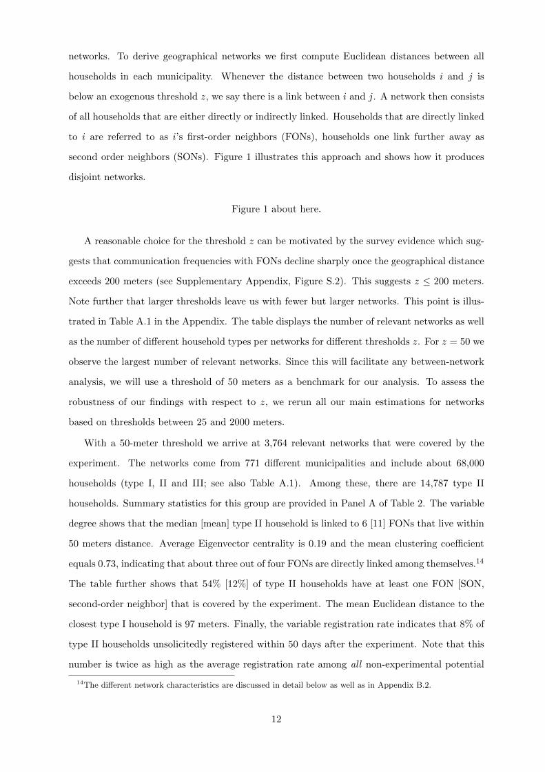
With a 50-meter threshold we arrive at 3,764 relevant networks that were covered by the
experiment. The networks come from 771 different municipalities and include about 68,000
households (type I, II and III; see also Table A.1). Among these, there are 14,787 type II
households. Summary statistics for this group are provided in Panel A of Table 2. The variable
degree shows that the median [mean] type II household is linked to 6 [11] FONs that live within
50 meters distance. Average Eigenvector centrality is 0.19 and the mean clustering coefficient
equals 0.73, indicating that about three out of four FONs are directly linked among themselves.14
The table further shows that 54% [12%] of type II households have at least one FON [SON,
second-order neighbor] that is covered by the experiment. The mean Euclidean distance to the
closest type I household is 97 meters. Finally, the variable registration rate indicates that 8% of
type II households unsolicitedly registered within 50 days after the experiment. Note that this
number is twice as high as the average registration rate among all non-experimental potential
14The different network characteristics are discussed in detail below as well as in Appendix B.2.
12

evaders (i.e., type II households inside and outside of networks covered by the experiment; see
Table 1, column (4)).15 Below we will show that the higher registration rate can be explained
by the presence of spillover effects from experimental to non-experimental households in these
networks.
Table 2 about here.
Panel B reports descriptive statistics at the network level. The network size, in the following
denoted by Nk, has a median [mean] of 6 [18] households. For each network k, we computed
variables that measure the treatment coverage: Totalk captures the rate of other households in
the experiment sample divided by Nk− 1. Similarly, Basek, Threatk and Controlk indicate the
ratios of other households targeted with a baseline, a threat mailing and untreated experimental
households, respectively. Using (Nk − 1) as denominator assures that the treatment rates vary
between zero and one.16 Table 2 shows that, from the perspective of a type II household in
an average network, 45% of the other households in a network were covered by the experiment;
21, 22 and 2% of the other network members were in the baseline, threat or control treatment,
respectively.17 The table further reports several measures of local treatment concentration and
‘homophily’ measures which are further discussed in Section 6.
Panel C of Table 2 presents summary statistics for census data at the municipality level. An
average municipality (hosting a relevant network) is populated by 1,790 inhabitants with a mean
labor income (wages and salaries) of 27,250 euro. 82% households live in single-family and two-
family homes. The household heads are on average 54 years old. The fraction of non-Austrians
citizens is low (5%) and a large majority of the population is Catholic (88%). We also observe
a high voter turnout at the 2006 national elections (77% on average).
5 Spillover Effects
5.1 Identifying Indirect Effects from the Experiment
Instead of studying the treatment responses of treated (type I) households, we focus on com-
pliance responses among the non-experimental population. We want to identify if and how a
15 One cannot directly compare these registration rates to those observed among type I households. As pointedout in Section 4.1, the latter sample contains a high fraction of households who were already complying beforethe experiment.
16 Below we will focus on the responses of type II households. Computing treatment rates relative to Nk wouldimpose an upper bound (at (Nk − 1)/Nk) which mechanically varies with the network size.
17The high treatment ratios reflect our focus on (relevant) networks with at least one experimental household.
13

type II household’s probability to register for license fees changes in response to the experimental
interventions. To estimate these spillover effects we consider the following model:
yik = α+ β0Totalk + β1Basek + β2Threatk + εik, (1)
where yik indicates if a type II household i from network k starts to comply with license fees
within 50 days after the experiment.18 The regressors measure the treatment rates at the network
level, i.e., the fraction of other households in the network that were part of the experimental
sample (Totalk), in the baseline (Basek) or in the threat treatment (Threatk), with Totalk =
Controlk +Basek + Threatk (see Section 4.2).19
The coefficients of interest, β1 and β2, measure the spillover effects on type II households’
propensity to start paying fees in response to a cet. par. increase in the network’s rate of base-
line and threat treatments, i.e., keeping constant Totalk. Put differently, these are the effects
from moving experimental households from the control group to one of the mailing treatments.
Alternatively, the effect of sending more mailings (while keeping constant the number of house-
holds in the control group) is given by β0 + β1 [β0 + β2] for the baseline [threat] treatment. The
coefficient β0 captures possible correlations between the experimental coverage and the average
probability of observing unsolicited registrations in a network; α depicts the baseline rate at
which type II households start to comply with license fees.
Identification. For a given experimental coverage, identification of β1 and β2 is obtained from
network-level variation in the treatment rates. The identifying assumption is that, conditional on
Totalk, variation in Basek and Threatk is as good as random: between networks with the same
coverage (Totalk), the assignment of the experimental households to the different treatments
varies exogenously. This is equivalent to a conditional independence assumption. Networks that
differ in experimental coverage are allowed to be different in unobservables which might affect
the propensity to comply (as reflected in β0). Controlling for Totalk, however, the variation in
the treatment ratios should be orthogonal to unobservables because the experiment randomly
assigned households to different treatments. The basic idea is simple: with random treatment
assignment in a given sample (i.e., among type I households), treatments should vary randomly
18The dummy only captures unsolicited registrations. Enforced registrations do not enter yik.19Below we show that specification (1) can be interpreted within a model of communication and learning in
networks (see Section 6). Alternative specifications in levels yield almost identical results as those reported below.However, estimations in levels turn out to be more sensitive to outliers related to a few very large networks.
14

in its sub-samples identified by our networks.20 The identifying assumption is credible because
– as underpinned by the balancing test in Fellner et al. (2013) and our Table 1 – randomization
in the experiment was successful.
To provide network-level evidence in support of our identifying assumption we estimate
models of the following structure: Basek = µbase0 +µbase1 Totalk +µbase2 xk + εbasek and Threatk =
µthreat0 + µthreat1 Totalk + µthreat2 xk + εthreatk , where xk is an observable characteristic that varies
at the network level. Our conditional independence assumption implies that, controlling for
Totalk, we should not find any correlation between observable network characteristics and our
key regressors: neither µbase2 nor µthreat2 should be statistically different from zero. Table 3
presents the results. Each entry in the table reports an estimated µ2-coefficient for a different
regressor xik from a separate regression. For columns (1) and (3), each estimation is based on
the sample of 3,764 relevant networks. None of the coefficients is statistically significant. In
columns (2) and (4), we repeat the exercise using different municipality characteristics. The
municipality-level estimates again yield no significant coefficients. The results thus support our
identifying assumption suggesting that, after controlling for experimental coverage, there is no
selection on observables.
Table 3 about here.
5.2 Basic Results
Using a linear probability model we estimate model (1) for all potential evaders from the non-
experimental population (type II households) in relevant networks with Totalk > 0.21 The
results, together with standard errors clustered at the network level, are reported in column (1)
of Table 4. The coefficients of interest are both positive and precisely estimated. The estimates
hardly change when we control for the networks’ experimental coverage linearly (as in column 1)
or non-parametrically, i.e., by including a set of 471 dummies for each value of Totalk (column 2).
The point estimates imply that a one percentage-point increase in the rate of the baseline [threat]
treatment increases the likelihood that an untreated potential evader registers by 0.25pp [0.35pp],
respectively. An F-test on the equality of β1 and β2 rejects the null that the two effects are equal.
The coefficient on Totalk is small and only weakly significant. The negative sign indicates that a
20It is worth noting that the partitioning of households into different networks is driven by the way settlementsare spread over the municipalities’ area. Effectively, the variation in our treatment variables thus comes from theexperiment in combination with characteristics such as population density and ‘gaps’ between settlements.
21Including networks with Totalk = 0 does not change the results since the other regressors in (1) also equalzero for networks with Totalk = 0.
15

higher experimental coverage of the network is correlated with a lower probability of unsolicited
registration among type II households.
To illustrate the size of the effect, consider the thought experiment where we move one
experimental household from the control to the threat treatment. For a median network with
N = 6, the additional mailing implies a 20pp increase in the threat treatment rate ( 16−1 = 0.2).
Our estimates imply that the additional threat mailing would increase the type II households’
probability to register by 7pp (0.2 × 0.35 = 0.07). On average, there will be just one type II
household in such a network (20% of N − 1 = 5; see Table A.1). We would therefore expect
a total spillover of 0.07 × 1 unsolicited registrations for license fees.22 Keeping constant the
experimental coverage, one additional threat [baseline] mailing thus increases the probability
of observing one additional registration among the untreated evaders in the network by 7pp
[5pp]. While the comparison of registration rates between the treated and the untreated sample
is problematic (see footnote 15), it is nevertheless worth noting that the total spillover effect
seems to be of a similar magnitude as the direct treatment effects on type I households (6.0pp
and 6.6pp for the baseline and threat treatment, respectively; see Table 1).
Table 4 about here.
Having detected a significant spillover from the experiment onto the non-experimental popu-
lation, it is important to note that we would miss these indirect treatment effects if we estimated
model (1) at the municipality rather than the network level. This point is documented in column
(3) of Table 4. For this regression we have assigned the sample from columns (1) and (2) (i.e.,
all potential evaders from geographic networks with Totalk > 0) into one network per munici-
pality. In line with this alternative network definition, we accordingly computed new treatment
rates for all 771 municipalities. Despite the fact that these municipalities are still fairly small
observational units (with a population of 1,790 individuals on average), we obtain estimates for
β1 and β2 that are very small and statistically insignificant.
In column (4) we enlarge the sample and include all type II households from all municipalities
with at least one experimental household. In this way, we obtain a sample of 62,064 non-
experimental potential evaders spread over 982 municipalities. Despite the larger sample, we
still obtain imprecisely estimated coefficients that are close to zero. Hence, the municipality
22For larger networks, the effect of one additional mailing on the treatment rates would of be smaller but thespillovers would spread to a larger number of potential evaders. It is straightforward to show that the model from(1) implies that the total expected spillover from sending one additional mailing into a network is independent ofthe network size.
16

seems to be an observational unit that does not allow us to capture the indirect treatment
effects that we detected at the level of geographical networks.
To sum up, Table 4 provides two first insights. First, there is a sizable spillover from the
experimental treatments on households that were not part of the experiment. Second, analyzing
this effect at the level of geographic networks (rather than municipalities) is important in order
to detect the spillover. Taken together, this suggests that geographical networks may be crucial
in shaping relevant parameters that affect compliance decisions. We will further explore this
case below. Before, we will discuss the robustness and some refinements of the spillover effect.
5.3 Robustness and Refinements
Alternative specifications. Table 5 reports the results from several exercises which assess
the robustness of our basic result. We first estimate model (1) using a probit model. Col-
umn (1) reports the marginal effects, computed at the mean of the independent variables. The
spillover effects are similar to those indicated by the LPM estimates and the effect size differs
again significantly between the two mailing treatments. In column (2) we return to the LPM
estimations and augment the basic specification by adding fixed effects at the municipality level.
As expected, this leaves our results unchanged.
Table 5 about here
Next we consider possible interferences with field inspections. To account for spillovers from
local enforcement activities (see Rincke and Traxler, 2011), the specification from column (3)
controls for the enforcement rate at the network level. Consistent with Rincke and Traxler
(2011), enforcement has a positive effect on the propensity to register. However, the point
estimates for our coefficients of interest are essentially identical to those from column (1) in
Table 4. In an additional step, we run our basic model excluding all networks in which at
least one household was targeted by a field inspector. This drops roughly 100 networks from
the sample.23 The results reported in column (4) show that the estimated coefficients remain
again unchanged. Finally, we test for potentially heterogenous spillover effects with respect to
municipality characteristics. The analysis reveals significant interaction effects for two variables:
the dwelling structure and the voter turnout. The magnitude of the spillover increases with the
23The number of non-experimental households in the sample drops by a larger share as the excluded networksare the larger ones. This is due to the fact that, cet. par., the probability to have at least one household targetedby a field inspector is increasing with the network size.
17

fraction of people living in single- and two-family dwellings (as compared to multi-family homes)
as well as with the turnout (see Table A.2 in the Appendix). The latter interaction might be
related to a higher social capital.
Different network assumptions. To understand the sensitivity of our findings with respect
to z, we computed geographical networks based on distance thresholds that vary between 25 and
2000 meters.24 We then replicate our estimates for the different samples of relevant networks.
Panel A in Table 6 reports the results for the basic model from (1) for different thresholds z.
The estimated coefficients turn out to be fairly stable for z < 500 meters. For larger values
of z, the coefficient on the baseline treatment starts to decline whereas the one on the threat
treatment remains large, however, with large standard errors.
In comparing the different estimation results, one has to take into account that a change in z
varies the number of relevant networks, the average network size, as well as the number of type II
households (see Table A.1). A first attempt to provide a meaningful comparison across samples
is provided in Panel B of Table 6. Here we normalize the coefficients on the two treatment rates
relative to the median network size (minus one). With this normalization, we get the effect
from sending one additional mailing to each relevant network on the register probability of a
type II household (in a median-sized network). Panel B shows that the effect from one mailing
monotonically declines with z. Given the results from Panel A, this decline is induced by the
fact that the median network size increases monotonically with z.
Table 6 about here
Panel C reports the results from a different thought experiment, which considers sending
a fixed amount of 1,000 additional baseline or threat mailings to relevant networks. Based
on our estimates and the network properties we then compute the total number of additional
registrations that we expect to be induced by the spillover effects from these mailings.25 For z =
50, for instance, the number of expected registrations that emerge from the indirect treatment
effect is 150 [232] for 1,000 additional baseline [threat] mailings, respectively. Panel C indicates
that the overall spillover starts to decline with z > 100. This observation fits the survey evidence
which showed that communication frequencies among FONs sharply declines in this range.
24Employing within-municipality distance matrices, we exclude links between networks from different munici-palities. This restriction becomes relevant for z ≥ 500 but affects only a small part of the sample.
25For the baseline mailings, this number is computed as follows: Number of Observations× 1,000Number of Networks
×β0+β1N−1
. Note that the effect is weighted with the total number of observations to account for the fact that thespillover applies to all type II households in the relevant networks.
18

Permutation test on networks. In principle, the results from Table 4 could be interpreted
in support of the idea that geographical networks of neighbors are a key unit for the information
transmission which shapes the spillover effects. A concern with this interpretation is that we
might simply have too little variation to detect any spillover when we estimate the regressions at
the municipality level. To address this concern and to provide further evidence that geographical
networks are crucial in determining the spillovers, we perform the following permutation test.
Within each of the 771 municipalities covered by the sample from our main specification
(Table 4, column 1), we randomly allocate all (type I, II and III) households into networks of
size N = 10.26,27 With this procedure, all households remain in their true municipalities but they
are randomly grouped in different networks, independently of their geographic location within
the municipality. For such a randomly generated network we then compute our regressors and
estimate model (1) on the sample from Table 4 (the 14,767 type II households). The results
from 1,000 iterations of this exercise are illustrated in Figure 2.
Figure 2 about here.
The figure displays the cumulative distribution functions of the estimated coefficients for
the baseline (β1, left panel) and the threat mailing (β2, right panel) as well as the true point
estimates. In less than the 5% of the cases (4.00% for β1; 1.60% for β2) the coefficients from
the permutation test are larger than the estimates from Table 4. This suggests that the results
from Table 4 are not simply driven by partitioning municipalities into smaller units. Instead,
the networks based on geographical distance seem to pick up a systematic spillover effect that
is shaped by interaction within these networks.
Spillovers within the experimental sample. Given our main results from above, it seems
natural to ask whether there are also spillovers within the experimental sample. If a type I
household’s treatment response depended on the treatment of other households in the network,
this would imply a violation of the stable unit treatment value assumption (SUTVA; see Imbens
and Wooldridge, 2009) for evaluating the direct effect of the experiment. To explore this case,
we focus on type I households and analyze whether the behavior of a treated household depends,
in addition to its own treatment, on the treatment rates in its network. Our analysis does not
yield any compelling evidence that treatment responses of type I households are influenced by
26For a municipality with, say, 1,017 households, we would randomly form 100 networks with 10 and onenetwork with the remaining 17 households.
27We obtain very similar results when we use N = 5 (close to the median network size, see Table 2) or N = 15(close to the 3rd quartile).
19

the treatment of their neighbors: controlling for the baseline and threat mailing rates does not
alter the estimates for the direct treatment effects of the mailings. Results are presented in
Table A.3 in the Appendix and suggest that, for the experimental sample, the direct treatment
effect dominates any indirect effect from the experiment.
5.4 Linking Direct and Indirect Treatment Effects
Receiving a mailing or starting to comply with licence fees is unobservable to other network
members. The spillover effect must therefore stem from the dispersion of information via com-
munication. Understanding the underlying patterns of communication – i.e., who passes on
which information – is important for optimal policy design that accounts for indirect treatment
effects (e.g. Banerjee et al., 2013; Beaman et al., 2015).
In our context one could imagine that type I households who do not start to comply in
response to a mailing might not talk about their treatment. Alternatively, if they communicated
with their neighbors, the information content might not trigger any effect on the neighbors’
compliance. The latter prediction can be derived from theories of conformity, imitation and
social norms (e.g. Akerlof, 1980; Bernheim, 1994) that all focus on behavioral interdependencies:
a change in the compliance of the treated household would be necessary to induce any indirect
treatment effect. In this case, we should not find any spillover from mailings that did not have any
direct treatment effect on compliance. If the indirect treatment effects were indeed contingent
on compliance responses of treated households, the spillover should be closely aligned with the
direct treatment effects. Our data do not support this case. Table 1 shows that the threat
produces roughly 10% more registrations than the baseline mailing (7.65/7.01). In contrast, the
estimates from Table 4 indicate that the indirect effect from a threat mailing is 40% larger than
the one from a baseline mailing (β2/β1 = 0.35/0.25).
To directly assess the role of direct treatment responses for the emergence of spillovers we
make use of the fact that more than a third of the type I households were actually complying
with license fees at the time of the experiment (see Section 4.1). Hence, these treated households
could, by definition, not switch from evasion to compliance. If behavioral changes were necessary
to induce an indirect effect, the mailings sent to compliant households should not produce
any spillover. To test this hypothesis, we re-run our basic regression model on the sample of
networks where all mailing targets were already complying with license fees before the treatment.
Column (1) in Table 7 reports the results.
20

The estimates indicate highly significant, positive spillovers from both mailing treatments.
The threat treatment triggers again a larger indirect effect than the baseline mailing (the equality
of coefficients is clearly rejected, F = 8.51). Note that this difference cannot be due to any
differential in the direct treatment effects. The model introduced in the following section shows
that the observation can be due to a treatment variation in the treated households’ likelihood
of passing on information or in the ‘relevance’ of the communicated information (or both).
Table 7 about here.
Column (2) replicates the estimation for the sample where the ex-ante compliance among
mailing targets was below 100%. When we account for the change in the estimated coefficient
on Totalk, the point estimates for the indirect effects are larger for the latter sample.28 This
observation is supported by the specification from column (3), which interacts the treatment
ratios with the average ex-ante compliance rate among the mailing targets in each network.
The negative coefficients on the two interaction terms suggest that the spillover, in particular
the one from the baseline mailing, decreases with the ex-ante compliance rate of the treated
households.29
To sum up, we find larger spillovers when there is scope for the treatments to directly
affect compliance behavior of the injection points. This mirrors a result from Banerjee et al.
(2013), who find that adopters of new technologies are crucial in the diffusion of the technology.
However, we detect sizable spillovers even when the mailings cannot alter the treated households’
compliance behavior. Behavioral changes among the targeted households are therefore not
necessary to induce the spillover. This means that the indirect treatment effects are not solely
shaped by behavioral interdependencies (as, e.g., in pure models of conformity). Building on
these findings, we now introduce a theoretical model of communication within networks that
further studies the dispersion of information and compliance.
28In column (1), for networks where all mailing recipients were already complying, we get β0 + β1 = 0.103[β0 + β2 = 0.272]. In these networks, a one percentage point increase in the rate of baseline [threat] mailings –that also increases the experimental coverage – increases a potential evader’s probability to register by 0.103pp[0.272pp]. In column (2), for networks where the mailings can directly alter the compliance behavior of the treatedhouseholds, the corresponding effect size is 0.205pp [0.297pp].
29We obtain very similar results when we interact the treatment rates with treatment-specific ex-ante compliancerates (analogously to, e.g., equation 5).
21

6 Communication in Networks
To analyze the spillover’s micro structure we introduce a theoretical model of communication
in networks. A network is formally defined as a collection of nodes N = {1, ..., N} and a set
of edges (links between the nodes) defined as Ξ ⊆ {(i, j)|i 6= j ∈ N}, where an element (i, j)
indicates that i and j are linked. A network can be described by its adjacency matrix A with
entries aij ∈ {0, 1} where aij = 1 indicates that i and j are linked. Networks in our setting are
undirected (i.e. if (i, j) ∈ Ξ, then also (j, i) ∈ Ξ), which means that the adjacency matrix A is
symmetric. The set of FONs of i is denoted by Ni = {j ∈ N|(i, j) ∈ Ξ}.30
The objective of our analysis is to understand how the different treatments and different
network structures interact in producing spillovers. In doing so, we distinguish four categories
of households, indicated by τ ∈ {a, b, c, d}: experimental (type I) households in the threat (a),
baseline (b) or control (c) treatment, as well as untreated (type II and III) households (d). Each
household has a ‘propensity’ to comply, pi. Given our objective, we are not tying ourselves to
any specific interpretations of p. The propensity might be shaped by extrinsic incentives (e.g.,
related to subjective beliefs about the sanction risk) or intrinsic motives (e.g., the strength of
a social norm which is malleable by neighbors’ views and decisions). If we denote the mean
propensities of all households of category τ in network k after receiving a possible treatment by
p0τk, we can make the following assumption:
Assumption A1: Before communication propensities satisfy p0ak > p0
bk > p0ck, ∀k.
Essentially, A1 amounts to saying that the treatments have a direct effect. After the treatment
(but before communication) households in the threat treatment have a higher propensity to
comply than those in the baseline treatment who in turn have a higher propensity to comply
than those of the control group (see Table 1 and Fellner et al., 2013).
Our model allows households to communicate for multiple rounds r. Specifically, in each
round, households communicate with their FONs about pri and update their compliance propen-
sities as follows:
pr+1i =
∑j∈Ni λij p
rj + λii p
ri∑
j∈Ni λij + λii, (2)
30Since the networks are undirected, ‘being a FON’ is a symmetric binary relation: if i is a FON of j, then j isalso a FON of i.
22

where λij ∈ R is the weight that i places on j’s opinion.31 Hence, a household’s updated
propensity is a weighted average of their own and their neighbors’ past propensities. This
updating process dates back to DeGroot (1974) and has been widely used in recent literature
(see, among others, DeMarzo et al., 2003; Acemoglu et al., 2010; Golub and Jackson, 2010, 2012;
Jadbabaiea et al., 2012).32
Updating of p will, by definition, affect compliance: households will stop evading whenever
their propensity pi exceeds a given threshold pi. The threshold is allowed to differ across house-
holds, reflecting heterogeneity in (risk) preferences, income, etc. The model then suggests that
treatment differences in spillover effects can be driven by two factors: differential treatment
effects on p and treatment specific communication frequencies captured by different weights λ.
To illustrate this point, consider the result discussed in Section 5.4: relative to the baseline mail-
ings, the threat produces a 10% larger direct treatment effect, but a 40% larger spillover effect.
The larger direct effect can be related to a differential increase in p. The larger indirect effect,
by contrast, suggests that households place higher weights on neighbors who were targeted with
a threat (instead of a basline) mailing (compare fn. 31). We will return to this point below.
Using matrix notation one can express the updating rule as pr+1 = Tpr, where T is a
‘communication matrix’. The ij-th entry of T is given by λijaij , i.e., it corresponds to the
weights λij from equation (2) if there is a link between i and j, otherwise it is zero. After
‘sufficiently many’ rounds of communication the updating process converges to a consensus in
which all agents in a network have the same p (DeGroot, 1974; DeMarzo et al., 2003). (This
does not imply that all households must display the same behavior, since preferences, and thus
the threshold pi, may differ across households.) The consensus propensity p∗ can be expressed
as a weighted average of all types’ initial propensities, i.e.,
p∗ =∑j∈N
ωjp0j , (3)
where ωj are weights which are further discussed below. In Appendix B we document that our
basic estimation model from (1) can be interpreted in terms of the consensus propensity from
equation (3). In particular, the coefficients β1 and β2 from model (1) will reflect the joint effect
31We allow for these weights to differ across neighbors. This might reflect any unobserved heterogeneity in therelationship between i and j. One might also assume that weights are treatment specific. A high weight placedon neighbors in the threat treatment (relative to the baseline treatment) could, for instance, capture the fact thatthese neighbors might be more likely to initiate communication.
32Empirical support for this form of learning has been found in lab experiments in some contexts (Chandrasekharet al., 2015; Grimm and Mengel, 2014), though in others the support has been weaker (Mobius et al., 2015).
23

of ωτ × p0τ , where ωτ is the average weight placed on agents of category a or b, respectively.33
These weights depend on the weights λij from equation (2), but also on the network positions
the different types occupy. How network position can affect spillovers will be the topic of the
next subsection.
6.1 Network Characteristics of Targeted Nodes
It can be shown (e.g., in Theorem 1 in DeMarzo et al., 2003), that the weights ω = (ω1, ..., ωN )
solve the row eigenvector equation
ωT = ω. (4)
Since the communication matrix T can be interpreted as the transition matrix of a finite, ir-
reducible, and aperiodic Markov chain, it has a unique eigenvalue equal to one and all other
eigenvalues with modulus smaller than one. The vector of weights ω is given by the row eigen-
vector corresponding to the largest eigenvalue of T. Network positions matter for ω, since they
matter for T (the ij-th entry of T is non-zero if and only if i and j are linked). In particular, a
household’s weight in the final consensus ωi will be closely related to i’s eigenvector centrality.34
In the special case where λij = λ,∀i, j (and hence T is proportional to A) an agent’s weight in
the final consensus ωi exactly coincides with her eigenvector centrality.
Under assumption A1, mailing-treated households with a higher eigenvector centrality should
then trigger a higher spillover and, cet. par., increase the impact of the intervention. To assess
this prediction, we analyze how the network position of mailing-treated households – the injec-
tion points – affects the size of the spillovers. Three network characteristics are of particular
interest in our context: (i) degree, (ii) clustering and (iii) eigenvector centrality.35 The degree
of a household simply reflects how many FONs this household has. As we assume that FONs
communicate with each other, the degree of household i measures to how many other households
i directly talks (and listens) to. The clustering coefficient reflects how ‘tightly knit’ communi-
ties are: it shows how many of household i’s neighbors are neighbors themselves. While degree
33In Appendix B we discuss more specific assumptions on the updating process which would lead to specificfunctional forms of ωτ and, in some cases, allow for identification of p0τ .
34Loosely speaking, eigenvector centrality measures with how many others a household connects, where con-nections to other ‘important’ households contribute more to the influence of the household in question than equalconnections to ‘unimportant’ households. Hence it is a recursively defined measure (see Appendix B.2 for theprecise definition). Google’s PageRank is a variant of the eigenvector centrality measure.
35A formal definition and further discussion of these characteristics is provided in Appendix B.2.
24

and clustering are important characteristics, our model suggests that it is the targeted node’s
eigenvector centrality that should be crucial in determining spillovers.
To confront these predictions with our data, we estimate models of the following structure:
yik = α+ β0 Totalk + β1Basek + β2 Threatk + γ1cXbaseck + γ2cX
threatck
+γ3c
(Xbaseck ×Basek
)+ γ4c
(Xthreatck × Threatk
)+ εik, (5)
where Xbaseck and X
threatck are the average values of the respective household characteristic c
(degree, clustering, or eigenvector centrality) among all injection points in the baseline or the
threat treatment in network k, respectively. We are primarily interested in the coefficients on the
interaction terms, γ3c and γ4c, which capture the impact of the injection points’ properties on the
spillover. Results from LPM estimates of equation (5) are presented in Table 8. Columns (1) to
(3) present interactions with the injection point’s degree, clustering and eigenvector centrality.
Column (4) presents a specification which includes interactions for all three characteristics.
Table 8 about here.
The estimates do neither indicate significant interactions with the degree nor with the clus-
tering coefficient of the injection points: in columns (1), (2) and (4), the estimated coefficients
on the interaction terms are small and imprecisely estimated. Consistent with theoretical predic-
tions, however, columns (3) and (4) reveal significant interactions with the eigenvector centrality.
Mailings targeted at ‘more central’ households within a network produce larger spillovers. A
one standard deviation increase in the eigenvector centrality of the injection points cet.par. in-
creases the spillover by about 25%.36 Hence, consistent with the model’s predictions, there is
scope to increase spillovers by targeting households with a higher eigenvector centrality within a
network. This result echoes previous findings by Banerjee et al. (2013) who found that the cen-
trality of the injection points in sampled networks constitutes a strong and significant predictor
of micro-finance adoption in Indian villages.
In the Appendix we further explore this result. We consider interactions with betweenness
centrality, which is positively correlated with eigenvector centrality (ρ = 0.4638) but clearly a
distinct measure. When we augment the specification from column (4) in Table 8 by including
36Recall first our average treatment effect from Section 5: a one percent higher baseline [threat] treatment rateincreases an evader’s likelihood to comply by 0.25pp [0.35pp]. The point estimates from column (4) indicate that,with a one standard deviation higher eigenvector centrality of the injection points (approximately 0.24), the effectsize would be 0.32pp [0.43pp].
25

betweenness centrality, we continue to find a positive interaction with the eigenvector centrality
(see Table A.4). We also examined interactions with average characteristics of all households
in a network (rather than the characteristics of injection points). Our results indicate that, by
and large, average network characteristics do not play a major role in shaping the spillovers (see
Table A.5). For instance, the average eigenvector centrality – in contrast to the centrality of the
injection points – does not significantly affect the indirect effects from the mailings. Average
network characteristics do not seem to provide useful information for the optimal targeting
of interventions. In our context, targeting should be based on the characteristics of potential
injection points.
6.2 Local Concentration of Interventions
Another important question for the optimal design of an enforcement intervention concerns the
effect of treatment concentration: is it more effective to locally concentrate mailings or to spread
treatments broadly within a network? The problem is illustrated in Figure 3, which displays
a case with high local treatment concentration, i.e., where treated households are FONs (left
panel), and another example where concentration is low (right panel). Where should we expect
larger spillovers? Intuition suggests that both targeting strategies could be reasonable. On
the one hand, a low concentration cet.par. means that more households will hear about the
treatment. Each of these households, however, is likely to hear only about one mailing and
to talk to many other untreated households. Hence, while many households will hear about a
mailing, the effect on each of their propensities may be too small to induce compliance. High
concentration resolves the latter issue but it will typically mean that less people hear about a
mailing.
Figure 3 about here.
The notion of local concentration is closely linked to the concept of homophily, which has re-
ceived a lot of attention in recent years across a variety of fields, including economics (Benhabib
et al., 2010), sociology (McPherson et al., 2001) or management (Borgatti and Foster, 2003).
Homophily refers to the empirical regularity that people tend to interact with ‘similar’ others.
This fact has been documented across many different dimensions of similarity (e.g., ethnicity,
gender, political opinions) and typologies of social ties (from intimate relations of friendship and
marriage to business collaborations and everyday interactions). Our notion of local treatment
26

concentration can be viewed as a homophily concept, where two neighbors are similar – in terms
of their (post-treatment) compliance propensity p0τ – if they are in the same treatment. The
random assignment of treatments assures that, conditional on being experimental participants,
local concentration will not reflect other household properties. While the exogeneity distin-
guishes local concentration from the inherently endogenous concept of homophily, it allows us
to isolate the network effects of similarity on information diffusion described in the model of
Golub and Jackson (2012).
Golub and Jackson (2012) employ the model from above to study whether convergence of
beliefs to the consensus p∗ is helped or hindered by homophily. According to their results, conver-
gence is hindered by (spectral) homophily implying that it is not optimal to locally concentrate
interventions.37 Under assumption A1 this means that spillovers decrease with the degree of
local concentration of the intervention. To asses this prediction empirically we consider three
different measures: (i) local concentration dummies, LCDbasek and LCDthreat
k , which equal one
if there are at least two injection points who are FONs and receive the same treatment (baseline
or threat); (ii) the inbreeding homophily index (IH-index) due to Coleman (1958) and employed
by Currarini et al. (2009), which is further discussed in Appendix B.3; (iii) a dummy indicating
whether the IH-index is positive.38 All of these measures vary at the network level. Table 2
(Panel b) suggests that in 17% of all networks there is at least one pair of FONs in the baseline
treatment. The summary statistics further reveal a lot of variation in the inbreeding homophily
index, with a majority of networks having a negative inbreeding homophily for the two mailing
treatments, but also a substantial share of networks having a positive IH index.
Following the structure of equation (5), we then estimate the model
yik = α+ β0 Totalk + β1Basek + β2Threatk + δ1 LCMbasek + δ2 LCM
threatk
+ δ3
(LCM base
k ×Basek)
+ δ4
(LCM threat
k × Threatk)
+ εik,
(6)
where LCM basek and LCM threat
k capture one of the three local concentration measures. To
address possible concern regarding the exogeneity of the local concentration of mailing targets
within a network, we will augment equation (6). More specifically, we control for the local
concentration of all experimental (type I) households, independently of their treatment. Condi-
tional on this ‘overall’ concentration of possible injection points, random treatment assignment
37See Theorem 1 in Golub and Jackson (2012) and our discussion in Appendix B.3.38The IH dummy avoids one downside of the IH index, which is that it is slightly biased downwards in small
networks (see Appendix B.3).
27

implies that the variation in the treatment specific concentration measures will be exogenous.39
The estimation results are presented in Table 9.
Table 9 about here.
The estimates suggest that local treatment concentration is associated with smaller spillovers.
A negative interaction is observed for all measures, for both mailing treatments, as well as for
the basic and the augmented version of equation (6). The interaction effects are only significant
for the IH-index (for the threat treatment) and the dummies capturing positive IH-indices (both
treatments). For the latter measures, we obtain the strongest results, both in terms of effect size
and precision: the point estimates from columns (5) and (6) indicate that the size of the spillover
in networks with a positive IH-index shrinks between 60% (threat) and 90% (baseline).40 To
assess the sensitivity of these interaction effects, we run estimations with local concentration
measures that pool the two mailing treatments (see Table A.6 in the Appendix). The exercise
increases statistical power and confirms the negative interaction effects: with a higher treatment
concentration, we get significantly smaller spillovers.
6.3 How ‘local’ are spillovers?
In this section we ask how far the mailing-induced communication content ‘travels’ in the net-
work. If new information does not travel very far in the network, then households with a closer
network distance to the injection points will tend to have higher (post communication) propensi-
ties than those far away.41 Spillovers may therefore be limited to households ‘closer’ to a treated
household.
Figure 4 about here.
Figure 4, which presents a hypothetical network, illustrates a case of local spillovers. In this
network, only household k receives a mailing. Since only k can start to spread the word, it will
always first reach k’s FONs (panel (b) in Figure 4). If the FONs do not pass on the information,
then any spillover will be limited to the treated households’ FONs. If they do pass it on, then
39The argument is similar to the conditional independence assumption discussed in Section 5.40The estimates from column (6) suggest that the average treatment effects for the baseline [threat] treatment
– a 0.25pp [0.35pp] increase in the probability to stop cheating – is 0.22pp [0.22pp] smaller in networks with apositive IH-index for the baseline [threat] treatment.
41Network distance, often also referred to as geodesic distance, refers to the length of the shortest path betweentwo agents (nodes).
28

the news will reach k’s SONs (panel (c) in Figure 4). Roughly speaking, if a treatment induces
more intensive communication, then more distant households (in terms of network distance) will
be reached via the spillover.
To analyze how far-reaching spillovers are in terms of network distance, we compute treat-
ment rates that distinguish between the treatments of a households’ first-, second- or a higher-
order neighbors (HONs). For the baseline treatment, for instance, we count the number of
i’s FONs, SONs, and HONs who received this treatment. Dividing these numbers by Nk − 1,
we obtain the rates Basehik for h ∈ {FON,SON,HON}. This approach assures the identity
Basek =∑
hBasehik (which analogously holds for the threat treatment). Hence, we estimate a
model variant to the one from equation (1), which now exploits variation between and within
networks:
yik = α+ β0Totalk +∑h
βh1Basehik +
∑h
βh2Threathik + εik. (7)
The discussion from above suggests that the estimated coefficients for βh1 and βh2 eventually do
not increase as we move from h = FON to h = SON and to h = HON .
Table 10 about here.
The results from LPM estimations of equation (7) are presented in column (1) of Table 10.
In general, the estimates support the hypothesis that a given mailing triggers a larger spillover
on household i if the mailing is targeted to ‘closer’ rather than more ‘distant’ neighbors of
i. The baseline and threat mailings both trigger sizable spillovers on the treated household’s
FONs. The point estimates indicate that the spillovers are around 50 to 60% lower among
SONs (with significantly different coefficients, F-statistics of 3.95 and 12.38 for the baseline
respectively the threat mailing). For the baseline treatment, the estimates do not indicate any
significant spillovers to higher-order neighbors. The spillover from this treatment is therefore
concentrated among FONs and SONs. For the threat treatment, this seems to be different.
Here we observe significant spillovers beyond SONs. In fact, the estimate for βHON2 is even
larger (but less precisely estimated) than βSON2 . The results are robust when we control for
the geographic distances to the nearest household treated with a baseline mailing or a threat
mailing (see column 2).42
42Results remain essentially unchanged if we also decompose the total rate of experimental participants (Totalk)by h.
29

The estimate indicate that the spillovers from the threat treatment have a larger scope than
those from the baseline treatment. One possible interpretation of this observation is that the
impact of the threat ‘lives on longer’, i.e., the treat induces more rounds of communication
than the baseline mailing. This would mean that households further away from the targeted
nodes will eventually hear about the threat but not about the baseline mailing. Another possible
interpretation is that the threat mailing simply leads to higher pre-communication propensities of
targeted nodes which can then lead to higher post-communication propensities by first-, second-,
and higher-order neighbors. Note that the first explanation is consistent with a higher weight
λ being placed on threat treated injection points – an idea that we discussed in Section 5.4, in
light of the stark differential in direct and indirect treatment effects between the baseline and
the threat treatment.
Naturally these results are sensitive to varying the distance threshold z: whether SONs or
HONs can be reached will depend on who is defined to be a SON or HON. What we robustly see
across all specifications for z, though, is that the threat letter reaches more distant neighbors
than the baseline treatment (see Table A.7 in the Appendix).
7 Conclusions
This paper studied how a randomized direct mailing campaign spills over onto compliance de-
cisions of untreated neighbors in geographic networks. Our research design builds on three
important blocks. First, by exploiting a large-scale field experiment which randomly assigns
targeted nodes to different treatments, we identify networks effects. Second, by applying a ge-
ographic network approach on comprehensive data that cover the universe of households from
rural Austria, we arrive at a large amount of networks with substantial variation in their char-
acteristics. Third, we formulate a model of communication in networks which captures how
the treatments’ impact is transmitted from treated to untreated nodes in a network. The the-
oretical framework then guides our empirical analysis on how the network positions of targeted
households affect social learning and, ultimately, the compliance spillover.
Our analysis identifies strong and precisely estimated spillover effects. In addition, the data
support two key predictions from the model. First, the spillover increases considerably with
the treated nodes’ eigenvector centrality (Banerjee et al., 2013, 2014). By contrast, neither
the nodes’ degree, the clustering coefficient nor any average network-level characteristics seem
to influence the effect size. Second, consistent with the idea that homophily impedes social
30

learning, we document that a higher local treatment concentration produces a significantly
smaller spillover (Golub and Jackson, 2012). Together with several null results from various
placebo network exercises, these findings indicate that the structure of our geographic networks
is useful to capture patterns of social learning among neighbors.
Our results carry important implications for the optimal targeting of enforcement policies
and all other interventions that play on word-of-mouth diffusion among neighbors. Our findings
suggest that one could, cet. par., greatly improve the intervention’s impact by targeting central
households and by spreading the treatment broadly within a network. The easy availability of
geographic information thereby facilitates the computation of neighborhood networks and allows
to implement this strategy at fairly low costs.
While our results clearly highlight the potential of a geographic network approach, more
research is needed to better understand when and how geographic proximity affects social learn-
ing. Future work needs to identify in which areas geographic networks play a more, less or an
equally important role as other types of networks. A first step in this direction is presented in
Beaman et al. (2015), who compare seeding based on geographic and elicited social networks
in the context of technology adoption in a developing country. Understanding how information
transmission in geographic networks compares to other networks in different contexts will also
help to clarify the effectiveness of geographic approaches in other contexts and policy domains.
31

References
Acemoglu, D., A. Ozdaglar, and A.ParandehGheibi (2010). Spread of (mis)-information in social net-
works. Games and Economic Behavior 70 (2), 194–227.
Akerlof, G. A. (1980). A Theory of Social Custom, of Which Unemployment May be One Consequence.
Quarterly Journal of Economics 94 (4), 749–75.
Alatas, V., A. Banerjee, A. G. Chandrasekhar, R. Hanna, and B. A. Olken (2012). Network Structure
and the Aggregation of Information: Theory and Evidence from Indonesia. NBER Working Paper
No. 18351.
Algan, Y., Q.-A. Do, N. Dalvit, A. Le Chapelain, and Y. Zenou (2015). How Social Networks Shape Our
Beliefs: A Natural Experiment among Future French Politicians. Mimeo, Sciences Po.
Allcott, H. (2011). Social norms and energy conservation. Journal of Public Economics 95 (9), 1082–1095.
Alstadsæter, A., W. Kopczuk, and K. Telle (2014). Social Networks and Tax Avoidance: Evidence from
a well-defined Norwegian Tax Shelter. Mimeo, Columbia University.
Ambrus, A., M. Mobius, and A. Szeidl (2014). Consumption risk-sharing in social networks. American
Economic Review 104 (1), 149–182.
Baldassari, D. and P. Bearman (2007). Dynamics of political polarization. American Sociological Re-
view 72, 784–811.
Banerjee, A., A. G. Chandrasekhar, E. Duflo, and M. O. Jackson (2013). The Diffusion of Microfinance.
Science 341, 1236498.
Banerjee, A., A. G. Chandrasekhar, E. Duflo, and M. O. Jackson (2014). Gossip: Identifying central
individuals in a network. NBER Working Paper No. 20422.
Bayer, P., S. Ross, and G. Topa (2008). Place of work and place of residence: Informal hiring networks
and labor market outcomes. Journal of Political Economy 116, 1150–1196.
Beaman, L., A. BenYishay, J. Magruder, and A. M. Mobarak (2015). Can network theory-based targeting
increase technology adoption? mimeo.
Beaman, L. and J. Magruder (2012). Who gets the job referral? Evidence from a social networks
experiment. American Economic Review 102 (7), 3574–3593.
Benhabib, J., A. Bisin, and M. O. Jackson (Eds.) (2010). The Handbook of Social Economics. Elsevier.
BenYishay, A. and A. M. Mobarak (2015). Social Learning and Incentives for Experimentation and
Communication. Working Paper, Yale University.
Berger, M., G. Fellner, R. Sausgruber, and C. Traxler (2015). Higher taxes, more evasion? Evidence
from border differentials in TV license fees. Working Paper, Hertie School of Governance.
Bernheim, B. D. (1994). A Theory of Conformity. Journal of Political Economy 102 (5), 841–77.
Borgatti, S. P. and P. C. Foster (2003). The network paradigm in organizational research: A review and
typology. Journal of Management 29(6), 991–1013.
Bruhin, A., L. Gotte, S. Haenni, and L. Jiang (2014). Spillovers of Prosocial Motivation: Evidence from
an Intervention Study on Blood Donors. IZA Discussion Paper No.8738.
Bursztyn, L., F. Ederer, B. Ferman, and N. Yuchtman (2014). Understanding Mechanisms Underlying
Peer Effects: Evidence From a Field Experiment on Financial Decisions. Econometrica 82 (4), 1273–
1301.
32

Cai, J., A. D. Janvry, and E. Sadoulet (2015). Social networks and the decision to insure. American
Economic Journal: Applied Economics 7 (2), 81–108.
Chandrasekhar, A. G., H. Larreguy, and J. P. Xandri (2015). Testing models of social learning on
networks: Evidence from a lab experiment in the field. Working Paper, Stanford University.
Chandrasekhar, A. G. and R. Lewis (2014). Econometrics of sampled networks. Mimeo, Stanford Uni-
versity.
Chetty, R., J. N. Friedman, and E. Saez (2013). Using Differences in Knowledge across Neighborhoods
to Uncover the Impacts of the EITC on Earnings. American Economic Review 103 (7), 2683–2721.
Coleman, J. S. (1958). Relational analysis: The study of social organizations with survey methods.
Human Organization 17 (4), 28–36.
Conley, T. and C. Udry (2010). Learning about new technology: Pineapple in Ghana. American Economic
Review 100 (1), 35–69.
Currarini, S., M. O. Jackson, and P. Pin (2009). An Economic Model of Friendship: Homophily, Minori-
ties, and Segregation. Econometrica 77 (4), 1003–1045.
DeGroot, M. (1974). Reaching a consensus. Journal of the American Statistical Association 69(345),
118–121.
DeMarzo, P., D. Vayanos, and J. Zwiebel (2003). Persuasion bias, social influence and uni-dimensional
opinions. Quarterly Journal of Economics 118(3), 909–968.
Dustmann, C., A. Glitz, and U. Schonberg (2015). Referral-based Job Search Networks. Review of
Economic Studies. forthcoming.
Fellner, G., R. Sausgruber, and C. Traxler (2013). Testing Enforcement Strategies in the Field: Threat,
Moral Appeal and Social Information. Journal of the European Economic Association 11, 634–660.
Goldenberg, J., H.Sangman, D. Lehman, and J. W. Hong (2009). The role of hubs in the adoption
process. Journal of Marketing 73(2), 1–13.
Golub, B. and M. O. Jackson (2010). Naive learning in social networks and the wisdom of crowds.
American Economic Journal: Microeconomics 2 (1), 112–149.
Golub, B. and M. O. Jackson (2012). How homophily affects the speed of learning and best-response
dynamics. Quarterly Journal of Economics 127 (3), 1287–1338.
Granovetter, M. (1973). The strength of weak ties. American Journal of Sociology 78, 1360–1380.
Grimm, V. and F. Mengel (2014). Experiments on belief formation in networks. Working Paper, Univer-
sity of Essex.
Hong, H., J. Kubik, and J. Stein (2005). Thy neighbor’s portfolio: Word-of-mouth effects in the holdings
and trades of money managers. Journal of Finance 60, 2801–2824.
Imbens, G. W. and J. M. Wooldridge (2009). Recent Developments in the Econometrics of Program
Evaluation. Journal of Economic Literature 47 (1), 5–86.
Jackson, M. O. (2008). Social and Economic Networks. Princeton University Press.
Jackson, M. O. (2015). The past and future of network analysis in economics. In The Oxford Handbook
on the Economics of Networks. Oxford University Press.
Jackson, M. O., T. Barraquer, and X. Tan (2012). Social capital and social quilts: Network patterns of
favor exchange. American Economic Review 102 (5), 1857–1897.
33

Jackson, M. O. and B. W. Rogers (2007). Relating network structure to diffusion properties through
stochastic dominance. BE Journal of Theoretical Economics 7 (1), 1–16.
Jacobs, J. (1961). The Death and Life of Great American Cities. New Work: Random House.
Jadbabaiea, A., P. Molavi, A. Sandroni, and A. Tahbaz-Salehi (2012). Non-bayesian social learning.
Games and Economic Behavior 76, 210–225.
Kaufmann, K. M., E. La Ferrara, and F. Brollo (2012). Learning about the enforcement of conditional
welfare programs: Evidence from the bolsa familia program in brazil. Working Paper, Department of
Economics, Bocconi University.
Kuhn, P., P. Kooreman, A. Soetevent, and A. Kapteyn (2011). The Effects of Lottery Prizes on Winners
and Their Neighbors: Evidence from the Dutch Postcode Lottery. American Economic Review 101 (5),
2226–47.
Landry, C., A. Lange, J. List, M. Price, and N. Rupp (2006). Toward an understanding of the economics
of charity: Evidence from a field experiment. Quarterly Journal of Economics 121 (2), 747–782.
Manski, C. F. (1993). Identification of endogenous social effects: The reflection problem. Review of
Economic Studies 60 (3), 531–542.
Marmaros, D. and B. Sacerdote (2006). How Do Friendships Form? Quarterly Journal of Eco-
nomics 121 (1), 79–119.
McPherson, M., L. Smith-Lovin, and J. Cook (2001). Birds of a feather: Homophily in social networks.
Annual Review of Sociology 27, 415–444.
Miguel, E. and M. Kremer (2004). Worms: Identifying Impacts on Education and Health in the Presence
of Treatment Externalities. Econometrica 72 (1), 159–217.
Mobius, M., T. Phan, and A. Szeidl (2015). Treasure Hunt: Social Learning in the Field. NBER Working
Paper No. 21014.
Mobius, M. and T. Rosenblat (2014). Social learning in economics. Annual Review of Economics 6 (1),
827–847.
Newman, M. J. (2006). Finding community structure in networks using the eigenvectors of matrices.
Physical Review E 74 (3), 036104.
Olken, B. A. (2007). Monitoring Corruption: Evidence from a Field Experiment in Indonesia. Journal
of Political Economy 115 (2), 200–249.
ORF Medienforschung (2006). Ausstattung der Haushalte 1986-2006. Osterreichischer Rundfunk, Wien.
Pomeranz, D. (2015). No taxation without information: Deterrence and self-enforcement in the value
added tax. American Economic Review 105 (8), 2539–69.
Rincke, J. and C. Traxler (2011). Enforcement Spillovers. Review of Economics and Statistics 93 (4),
1224–1234.
34

Tables
Table 1: Summary statistics for type I and type II households (raw data)
Type I Type II
Experimental Sample Non-Experimental Sample
Control Base Threat Potential Evaders
Registration rate 0.0109 0.0701 0.0765 0.0425
(0.1041) (0.2552) (0.2659) (0.2018)
Ex-ante compliance 0.3625 0.3627 0.3752 –
(0.4809) (0.4808) (0.4842) –
Male 0.8363 0.8375 0.8379 0.8156
(0.0418) (0.0423) (0.0423) (0.0430)
Age 40.04 39.67 39.28
(13.00) (12.47) (12.11)
Degree 19.87 21.66 21.42
(52.09) (55.39) (55.83)
Clustering 0.67 0.68 0.67
(0.40) (0.39) (0.69)
Eigenvector centrality 0.31 0.31 0.31
(0.24) (0.24) (0.24)
Number of households 1,371 11,177 11,078 131,884
Notes: Summary statistics (mean and standard deviation in parenthesis) for potential evadersin the experimental (type I) and non-experimental sample (type II households). The first threecolumns present sample means for the three treatment arms of the experiment (Control, Base andThreat), the last column includes type II households. Information on age (reported in columns1–3) is only available for a subset of 2,778 households.
35
Table 2: Summary statistics for relevant networks, z = 50 meters
(A) Household level (14,787 type II households)
mean sd median 1st quart 3rd quart
Degree 11.26 22.35 6 3 11
Clustering 0.73 0.29 0.80 0.60 1
Eigenvector Centrality 0.19 0.00 0.34 0.13 0.41
FON in experiment 0.54 0.50 1 0 1
FON w/ Base 0.27 0.44 0 0 1
FON w/ Threat 0.26 0.44 0 0 1
FON w/ Control 0.07 0.26 0 0 0
SON in experiment 0.12 0.33 0 0 0
SON w/ Base 0.05 0.21 0 0 0
SON w/ Threat 0.05 0.23 0 0 0
SON w/ Control 0.01 0.10 0 0 0
Spatial distance to closest neighbor...
... in experiment 96.73 144.54 45.36 2.87 115.03
... w/ Base 294.00 738.15 86.13 35.53 243.84
... w/ Threat 317.27 741.38 91.37 34.28 273.04
... w/ Control 681.05 1079.82 115.73 297.84 737.43
Registration rate 0.08 0.27 0 0 0
(B) Network level (3,764 networks)
Network size (Nk) 17.98 45.48 6 3 14
Treatment Rates:
Totalk 0.45 0.33 0.40 0.39 0.67
Basek 0.21 0.28 0.10 0.00 0.33
Threatk 0.22 0.29 0.10 0.00 0.33
Controlk 0.03 0.11 0.00 0.00 0.00
Local Treatment Concentration:
LCDbase 0.17 0.38 0 0 0
LCDthreat 0.17 0.38 0 0 0
LCDall (any treatment) 0.25 0.43 0 0 1
IHbase -0.17 0.28 -0.04 -2.00 0.41
IHthreat -0.17 0.28 -0.04 -1.00 0.69
IHall (any treatment) -0.32 0.35 -0.20 -2.00 0.79
(C) Municipality level (771 municipalities)
Population 1,790 1,006 1,570 1,060 2,365
Labor Income 27,250 2,172 26,936 25,977 28,332
Average Age 53.73 20.10 51.5 36.75 69.25
Non-Austrian Citizens 0.05 0.04 0.04 0.02 0.07
Catholic 0.88 0.10 0.91 0.86 0.95
1- or 2-Family Dwellings 0.82 0.14 0.84 0.75 0.92
Voter Turnout 0.76 0.07 0.77 0.72 0.81
Notes: Panel A presents summary statistics at the household level for all potential evaders in the non-experimental sample (type II households) that are located in networks with at least one experimentalparticipant (type I household). Panel B reports (unweighted) network level statistics for these relevantnetworks. Panel C considers several municipality characteristics (unweighted, at municipality level). FONand SON abbreviate First and Second Order Neighbors, respectively. LCD’s are Local ConcentrationDummies and IH denotes inbreeding homophily (see Section 6). Spatial distance is measured in meters.
36

Table 3: Balancing Tests
(1) (2) (3) (4)
Basek Basek Threatk Threatk
Network Size -0.0000 -0.0000
(0.0000) (0.0000)
Clustering 0.0056 -0.0095
(0.0136) (0.0135)
Degree 0.0001 -0.0001
(0.0001) (0.0001)
Eigenvector Centrality 0.0102 -0.0071
(0.0179) (0.0178)
Population 0.0000 -0.0000
(0.0000) (0.0000)
Labor Income 0.0000 -0.0000
(0.0000) (0.0000)
Average Age -0.0003 0.0004
(0.0009) (0.0009)
Catholic 0.0015 0.0035
(0.0087) (0.0092)
Non-Austrian Citizens -0.0252 0.0476
(0.0315) (0.0334)
1- or 2-family dwellings -0.0006 0.0050
(0.0107) (0.0116)
Voter Turnout 0.0120 -0.0122
(0.0289) (0.0301)
Observations 3,764 771 3,764 771
Notes: The table reports estimates for different µ2 coefficients from regressions of Basek =µbase0 + µbase1 Totalk + µbase2 xk + εbasek and Threatk = µthreat0 + µthreat1 Totalk + µthreat2 xk +
εthreatk , where xk is a network level variable in columns (1) and (3) and a municipal levelvariable in columns (2) and (4). Each estimate in the table is obtained from a differentregression based on 3,764 (network-level) or 771 observations (municipality-level). Robuststandard errors are in parentheses. None of the coefficients is significant at conventional levels.
37

Table 4: Basic results
(1) (2) (3) (4)
Networks with z = 50m Municipality level
Basek 0.2491??? 0.2450??? 0.0073 0.0221
(0.0386) (0.0385) (0.3038) (0.1378)
Threatk 0.3533??? 0.3491??? -0.0495 -0.0061
(0.0394) (0.0393) (0.3419) (0.1541)
Totalk -0.0581? 0.2736 0.2123
(0.0335) (0.3277) (0.1487)
Constant 0.0313??? 0.0199??? 0.0463??? 0.0228???
(0.0027) (0.0069) (0.0039) (0.0010)
F-test for H0 : β1 = β2 13.47 12.27
Totalk Fixed Effects No Yes No No
Observations 14,787 14,787 14,787 62,064
Networks 3,764 3,764 771 982
R2 0.0560 0.0971 0.0150 0.0176
Notes: The table presents the results from LPM estimations of equation (1). In column (2) the variable Totalk entersnon-parametrically by including a set of dummies for each value of Totalk. Column (3) uses the sample from the firsttwo specifications but assumes that the network is defined by the municipality. Column (4) maintains this assumptionbut enlarges the sample including all potential evaders with at least one experimental participant in their municipality.Standard errors, clustered at the network (columns 1 and 2) or municipality level (3 and 4), are reported in parentheses.???/??/? indicates significance at the 1%/5%/10%-level, respectively.
Table 5: Robustness of basic results
(1) (2) (3) (4)
Probit Municipality Field Inspections
Fixed Effects
Basek 0.1973??? 0.2212??? 0.2495??? 0.2531???
(0.0551) (0.0443) (0.0386) (0.0390)
Threatk 0.2419??? 0.3341??? 0.3532??? 0.3593???
(0.0550) (0.0454) (0.0394) (0.0398)
Totalk -0.0548 -0.0769? -0.0582? -0.0615?
(0.0542) (0.0415) (0.0335) (0.0339)
Enforcement Rate – – 0.0040??? –
(0.0005)
Constant -0.0639 0.0400??? 0.0304??? 0.0294???
(0.0589) (0.0042) (0.0027) (0.0030)
Observations 14,787 14,787 14,787 12,891
Networks 3,764 3,764 3,764 3,657
R2 0.0774 0.1101 0.0570 0.0600
Notes: Column (1) is based on a Probit estimation of equation (1). It reports marginal effects evaluated at the meanof the indepedent variables. Columns (2)–(4) are estimated using a linear probability model. Column (2) includes fixedeffects at the municipality level. Column (3) controls for the rate of enforcement from field inspections. Column (4)excludes all networks with an enforcement rate greater than zero. Standard errors, clustered at the network level, arereported in parentheses. ???/??/? indicates significance at the 1%/5%/10%-level, respectively.
38

Table 6: Different distance (network) assumptions
(1) (2) (3) (4) (5) (6) (7) (8) (9)Threshold z = 25 50 75 100 250 500 1000 1500 2000
Panel A. Estimation Results
Basek 0.2454??? 0.2491??? 0.2687??? 0.2775??? 0.2730??? 0.2668?? 0.2271 0.0759 -0.0673(0.0336) (0.0386) (0.0573) (0.0545) (0.0798) (0.1359) (0.2594) (0.3699) (0.4851)
Threatk 0.3106??? 0.3533??? 0.3940??? 0.3910??? 0.3569??? 0.5063??? 0.4910? 0.4342 0.2788(0.0341) (0.0394) (0.0590) (0.0559) (0.0823) (0.1362) (0.2588) (0.3582) (0.4559)
Totalk 0.0198 -0.0581? -0.1056?? -0.1207?? -0.1207? -0.2039? -0.1903 -0.0943 0.0485(0.0313) (0.0335) (0.0524) (0.0476) (0.0716) (0.1230) (0.2379) (0.3349) (0.4357)
Constant 0.0187?? 0.0314??? 0.0348??? 0.0386??? 0.0421??? 0.0430??? 0.0446??? 0.0447??? 0.0444???
(0.0078) (0.0027) (0.0021) (0.0020) (0.0018) (0.0016) (0.0015) (0.0015) (0.0015)
Observations 5,236 14,787 23,473 29,012 41,347 50,488 58,298 60,320 61,351Networks 3,198 3,764 3,319 2,990 2,113 1,554 1,169 1,073 1,020R2 0.0782 0.056 0.0369 0.0264 0.0151 0.0114 0.0081 0.0077 0.0078
Panel B. Average individual effect from one additional mailing into each network:
Base 0.1231 0.0498 0.0336 0.0277 0.0105 0.0039 0.0014 0.0004 -0.0003Threat 0.1550 0.0707 0.0492 0.0391 0.0137 0.0075 0.0031 0.0023 0.0013
Panel C. Total spillover from 1,000 additional mailing, spread over all networks:
Base 217.15 150.01 144.21 152.08 114.54 30.09 11.53 -5.40 -5.42Threat 270.55 231.91 254.91 262.18 177.74 144.49 94.30 99.49 94.20
Notes: Panel A reports the results from LPM estimations of equation (1) for the different samples of type II households that emergefor different levels of the distance threshold z. Standard errors, clustered at the network level, are in parentheses. ???/??/? indicatessignificance at the 1%/5%/10%-level, respectively. Panel B presents the effect of sending one additional baseline [threat] mailinginto each network on a type II household’s probability to register. The effect is derived from the point estimates from Panel A and
given by β1N−1
[ β2N−1
], where we use the respective median network size for N . Panel C computes the expected spillover from sending
a fixed number of 1,000 additional baseline [threat] mailings into the networks covered by the respective sample. For the baseline
mailings, the total number of expected registrations is computed as follows: Number of Observations× 1,000Number of Networks
× β0+β1N−1
.
The effect is weighted with the total number of observations to account for the fact that the spillover applies to all type II householdsin these networks.
39
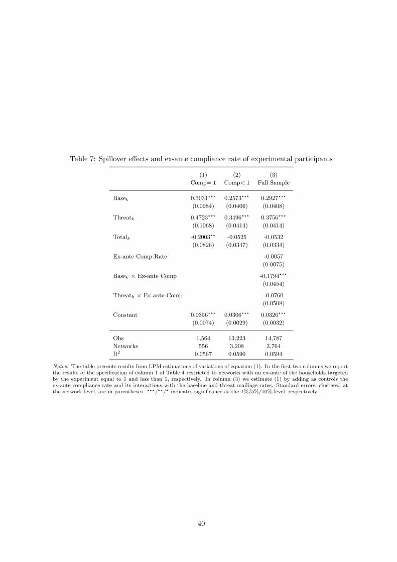
Table 7: Spillover effects and ex-ante compliance rate of experimental participants
(1) (2) (3)
Comp= 1 Comp< 1 Full Sample
Basek 0.3031??? 0.2573??? 0.2927???
(0.0984) (0.0406) (0.0408)
Threatk 0.4723??? 0.3496??? 0.3756???
(0.1068) (0.0414) (0.0414)
Totalk -0.2003?? -0.0525 -0.0532
(0.0826) (0.0347) (0.0334)
Ex-ante Comp Rate -0.0057
(0.0075)
Basek × Ex-ante Comp -0.1794???
(0.0454)
Threatk × Ex-ante Comp -0.0760
(0.0508)
Constant 0.0356??? 0.0306??? 0.0326???
(0.0074) (0.0029) (0.0032)
Obs 1,564 13,223 14,787
Networks 556 3,208 3,764
R2 0.0567 0.0590 0.0594
Notes: The table presents results from LPM estimations of variations of equation (1). In the first two columns we reportthe results of the specification of column 1 of Table 4 restricted to networks with an ex-ante of the households targetedby the experiment equal to 1 and less than 1, respectively. In column (3) we estimate (1) by adding as controls theex-ante compliance rate and its interactions with the baseline and threat mailings rates. Standard errors, clustered atthe network level, are in parentheses. ???/??/? indicates significance at the 1%/5%/10%-level, respectively.
40

Table 8: Spillover effects and injection points
(1) (2) (3) (4)
Degree Clustering Centrality All Measures
Basek 0.2533??? 0.0997 0.2526??? 0.0507
(0.0390) (0.0641) (0.0417) (0.0789)
Threatk 0.3531??? 0.2152??? 0.3594??? 0.1304
(0.0399) (0.0694) (0.0426) (0.0841)
Totalk -0.0616? -0.0368 -0.0753?? -0.0435
(0.0334) (0.0326) (0.0342) (0.0335)
Basek × Degreebase -0.0009 -0.0002
(0.0022) (0.0023)
Threatk × Degreethreat 0.0024 0.0024
(0.0024) (0.0026)
Degreebase -0.0002 -0.0002
(0.0003) (0.0004)
Degreethreat -0.0007??? -0.0006
(0.0002) (0.0004)
Basek × Clusteringbase 0.0236 0.0705
(0.0430) (0.0499)
Threatk × Clusteringthreat 0.0323 0.0831
(0.0461) (0.0542)
Clusteringbase -0.0136? 0.0030
(0.0073) (0.0085)
Clusteringthreat -0.0209??? 0.0052
(0.0075) (0.0092)
Basek × Centralitybase 0.1896?? 0.2714??
(0.0895) (0.1096)
Threatk × Centralitythreat 0.2157?? 0.3426???
(0.0974) (0.1179)
Centralitybase 0.0442? 0.0160
(0.0255) (0.0296)
Centralitythreat 0.0094 -0.0192
(0.0255) (0.0290)
Obs 14,787 14,431 14,787 14,431
Networks 3,764 3,764 3,755 3,755
R2 0.0574 0.0567 0.0607 0.0621
Notes: The table presents results from LPM estimations of variations of equation (5). In the first, second and thirdcolumn the network characteristic of injection points included in the model is the degree, the clustering coefficient andthe eigenvector centrality. In the last column all three measures are included. Standard errors, clustered at the networklevel, are in parentheses. ???/??/? indicates significance at the 1%/5%/10%-level, respectively.
41

Table 9: Spillover effects and local treatment concentration
LCDummies IH-Index IH-Dummies
(1) (2) (3) (4) (5) (6)
Basek 0.2617??? 0.2582??? 0.1648??? 0.1712??? 0.2865??? 0.2871???
(0.0394) (0.0392) (0.0476) (0.0527) (0.0406) (0.0407)
Threatk 0.3717??? 0.3684??? 0.2446??? 0.2510??? 0.4075??? 0.4080???
(0.0404) (0.0403) (0.0493) (0.0555) (0.0416) (0.0417)
Totalk -0.0417 -0.0375 -0.0396 -0.0454 -0.0838?? -0.0836??
(0.0329) (0.0328) (0.0328) (0.0401) (0.0340) (0.0340)
Basek × LCDbasek -0.0502 -0.0488
(0.0508) (0.0509)
Threatk × LCDthreatk -0.0629 -0.0614
(0.0525) (0.0529)
LCDbasek -0.0059 -0.0000
(0.0118) (0.0125)
LCDthreatk -0.0186? -0.0124
(0.0112) (0.0121)
LCDallk -0.0129?
(0.0074)
Basek × IHbasek -0.0045 -0.0012
(0.0555) (0.0571)
Threatk × IHthreatk -0.1112? -0.1080?
(0.0612) (0.0625)
IHbasek -0.0924?? -0.0876?
(0.0439) (0.0470)
IHthreatk -0.0316 -0.0266
(0.0502) (0.0540)
IHallk -0.0076
(0.0299)
Basek × IHDbasek -0.2061??? -0.2161???
(0.0576) (0.0597)
Threatk × IHDthreatk -0.2068??? -0.2143???
(0.0594) (0.0617)
IHDthreatk 0.0304??? 0.0306???
(0.0061) (0.0061)
IHDbasek 0.0188??? 0.0190???
(0.0060) (0.0061)
IHDallk 0.0045
(0.0076)
R2 0.0596 0.0598 0.0596 0.0596 0.0602 0.0602
Notes: The table presents results from LPM estimations of variations of model equation (6). In columns 1-2, the localconcentration measures are the local concentration dummies (LCD). In columns 3-4, the local concentration measuresare inbreeding homophily indexes (IH-index) and in columns 5-6, the inbreeding homophily dummies (IH-dummies). Allestimates are based on 14,787 observations from 3,764 networks. Standard errors, clustered at the network level, are inparentheses. ???/??/? indicates significance at the 1%/5%/10%-level, respectively.
42

Table 10: How local are spillovers?
(1) (2)
BaseFON 0.2643??? 0.2620???
(0.0388) (0.0328)
BaseSON 0.1424?? 0.1372??
(0.0668) (0.0670)
BaseHON 0.0141 0.0022
(0.0699) (0.0783)
ThreatFON 0.3665??? 0.3670???
(0.0396) (0.0400)
ThreatSON 0.1439?? 0.1427??
(0.0678) (0.0680)
ThreatHON 0.3204??? 0.3197??
(0.0796) (0.0800)
Total -0.0475 -0.0483
(0.0329) (0.0329)
Distance to nearest Base - -0.0000???
(0.0000)
Distance to nearest Threat - -0.0000
(0.0000)
F-tests:
BaseFON=BaseSON 3.95 4.13
BaseFON=BaseHON 15.39 15.94
BaseSON=BaseHON 2.39 2.49
ThreatFON=ThreatSON 12.38 12.54
ThreatFON=ThreatHON 0.38 0.40
ThreatSON=ThreatHON 3.41 3.42
Obs 14,787 14,787
Networks 3,764 3,764
Notes: The table presents results from LPM estimations of equation (7). Column(2) controls for distances to the nearest household treated with a baseline and athreat mailing, respectively. Standard errors, clustered at the network level, are inparentheses. ???/??/? indicates significance at the 1%/5%/10%-level, respectively.
43

Figures
Figure 1: Illustration of geographical networks
Notes: The figure presents an example of two disjoint networks for the case z = 50 meters.
Figure 2: Permutation tests – Distribution of estimated coefficients
0
0.2
0.4
0.6
0.8
1
cum
ulat
ive
dist
ribut
ion
func
tion
-0.40 -0.20 0.00 0.20 0.40Coefficients on baseline mailing rate for randomly generated networks
0
0.2
0.4
0.6
0.8
1
cum
ulat
ive
dist
ribut
ion
func
tion
-0.40 -0.20 0.00 0.20 0.40Coefficients on threat mailing rate for randomly generated networks
Notes: The figures present the cumulative distribution function of the coefficients on the baseline (left panel) and threat(right) mailing rates, obtained from the permutation test described in Section 5.3. The red vertical lines represent thecoefficients on the baseline and the threat mailing rates obtained from estimating model (1).
44

Figure 3: Local treatment concentration
Local Concentration is high Local Concentration is low
Notes: The figure shows two networks with the same structure but different degrees of local treatment concentration.There are three types represented in this picture. The dark nodes could represent type A (threat), the lighter nodes typeB (base) and the empty nodes untreated, non-experimental agents (type D). In the left panel, households of the sametype tend to be neighbors, while households in the right panel tend to be neighbors with households of a different type.
Figure 4: How local are spillovers?
(a) (b) (c) (d)
2
3
1
4
k
1
2
3
1
4
k
1
2
3
1
4
k
1
2
3
1
4
k
1
Notes: The figure shows targeted household k with its first-, second-, third-, and fourth-order neighbors (indicated bynumbers 1,2,3,4) in a hypothetical network. Panel (a) represents the time before communication starts where only kknows about its letter, in (b) the news has spread to k’s FONs, in (c) to her SONs, etc. Note that each time the messagespreads its impact becomes smaller: in (c) for instance, the SON of k learns about the letters but also about the factthat k’s FONs – with who she communicates – did not receive a letter.
45

Appendix A Additional Figures and Tables
Table A.1: Properties of relevant networks for different distance thresholds z.
Network threshold z = 25 50 75 100 250 500 1000 1500 2000
Networks 3,198 3,764 3,319 2,990 2,113 1,554 1,169 1,073 1,020
Mean Network Size 5.94 17.98 32.93 45.13 90.40 151.95 232.91 261.66 279.54
Type I HHs 4,481 11,794 15,343 17,172 20,699 22,332 23,097 23,227 23,296
Type II HHs 5,236 14,787 23,473 29,012 41,347 50,488 58,298 60,320 61,351
Type III HHs 9,277 41,107 70,482 88,742 128,959 163,311 190,882 197,214 200,483
Notes: A network becomes relevant for studying spillovers if there is at least one type I household and at least one typeII household.
Table A.2: Interactions with municipality characteristics
(1) (2) (3) (4) (5) (6) (7)Variable M = Income Catholic Population Age Non-Austrians Turnout Dwellings
Totalk -0.0571? -0.0561? -0.0586? -0.0604? -0.0569? -0.0457 -0.0544(0.0335) (0.0336) (0.0335) (0.0334) (0.0335) (0.0333) (0.0334)
Basek 0.1607 0.6840??? 0.2494??? 1.4187?? 0.2123 -0.4590?? 0.0354(0.2029) (0.2616) (0.0496) (0.6700) (0.3288) (0.2096) (0.1060)
Threatk 0.3223 0.5068?? 0.3525??? 0.1773 -0.2460 -0.1770 0.0443(0.2370) (0.2455) (0.0537) (0.6986) (0.3085) (0.2262) (0.1206)
Basek × M -0.0000 -0.4823? 0.0000 -0.0244? 0.0392 0.9881??? 0.2787??
(0.0000) (0.2859) (0.0000) (0.0139) (0.3526) (0.2924) (0.1319)
Threatk × M -0.0000 -0.1695 0.0000 0.0037 0.6427? 0.7402?? 0.4042???
(0.0000) (0.2690) (0.0000) (0.0146) (0.3305) (0.4855) (0.1517)
M 0.0000 -0.0070 -0.0000 -0.0018 0.0508 0.0185 -0.0089(0.0000) (0.0269) (0.0000) (0.0018) (0.0525) (0.0428) (0.0151)
R2 0.0521 0.0568 0.0560 0.0569 0.0571 0.0605 0.0585
Notes: The table reports results from LPM estimates of extension of equation (1) where the treatment rates are interactedwith a municipality variable M (see Panel (C) in Table 2). All estimates are based on 14,787 observations from 3,764networks. A constant term is included but estimates are not reported. Standard errors, clustered at the network level,are reported in parentheses. ???/??/? indicates significance at the 1%/5%/10%-level, respectively.
46

Table A.3: Spillover effects within the experiment
(1) (2) (3) (4)
Basei 0.0591??? 0.0597??? 0.0475??? 0.0487???
(0.0037) (0.0038) (0.0050) (0.0051)
Threati 0.0656??? 0.0660??? 0.0536??? 0.0546???
(0.0037) (0.0039) (0.0051) (0.0052)
Basek - 0.0086 - 0.0199
(0.0251) (0.0622)
Threatk - 0.0118 - 0.0072
(0.0245) (0.0603)
Totalk - -0.0580?? - -0.0418
(0.0230) (0.0577)
Constant 0.0109??? 0.0293??? 0.0103??? 0.0360???
(0.0028) (0.0034) (0.0038) (0.0060)
Observations 23,626 23,626 11,794 11,794
Networks – 10,535 – 1,530
R2 0.0030 0.009 0.003 0.007
Notes: The table reports LPM estimates for the direct treatment effects in the experimental sample (type I house-holds). Baselineti and Threati indicate a dummy equal to 1 if type I houeshold i was in the baseline or threattreatment, respectively. In columns (1) and (2) we run regressions on all type I households included in our raw data,in column (3) and (4) we consider only type I households from relevant networks with z = 50 as defined above (seeSection 4.2). Columns (2) and (4) add controls for the treatment rates at the network level. In column (1) and (3)robust standard errors are in parentheses, in column (2) and (4) standard errors are clustered at the network level.???/?? indicates significance at the 1%/5%-level, respectively.
47

Table A.4: Spillover effects and injection points: Betweenness centrality
(1) (2) (3)
Betweenness Basic specification (3) All measures
Basek 0.2535??? 0.0507 0.0343
(0.0392) (0.0790) (0.0821)
Threatk 0.3651??? 0.1304 0.1607?
(0.0392) (0.0841) (0.0821)
Totalk -0.0566 -0.0435 -0.0427
(0.0336) (0.0335) (0.0336)
Basek × Betweennessbase -0.1552 -0.0768
(0.1291) (0.1329)
Threatk × Betweennessthreat -0.1923? -0.1431
(0.1169) (0.1194)
Basek × Degreebase -0.0002 -0.0003
(0.0023) (0.0023)
Threatk × Degreethreat 0.0024 0.0025
(0.0026) (0.0026)
Basek × Centralitybase 0.2714?? 0.3151???
(0.1096) (0.1156)
Threatk × Centralitythreat 0.3426??? 0.2852??
(0.1179) (0.1226)
Basek × Clusteringbase 0.0705 0.0862?
(0.0499) (0.0515)
Threatk × Clusteringthreat 0.0831 0.0739
(0.0542) (0.0557)
Observations 14,787 14,431 14,431
R2 0.0571 0.0621 0.0627
Networks 3,764 3,755 3,755
Notes: The table replicates Table 8 by including betweenness centrality in equation (5). (Betweenness centrality ofan injection point i is defined as the share of shortest paths between any two households within the network passingthrough i.) Standard errors, clustered at the network level, are in parentheses. ???/??/? indicates significance at the1%/5%/10%-level, respectively.
48

Table A.5: Spillover effects and average network characteristics
Variable Ak = Degree Centrality Clustering Diameter Charpathlength Assortativity
(1) (2) (3) (4) (5) (6)
Basek 0.2526??? 0.2253??? 0.2872??? 0.2571??? 0.2581??? 0.1971??
(0.0390) (0.0659) (0.0459) (0.0404) (0.0403) (0.0936)
Threatk 0.3498??? 0.2548??? 0.3953??? 0.3710??? 0.3765??? 0.2799???
(0.0399) (0.0696) (0.0467) (0.0419) (0.0417) (0.0921)
Totalk -0.0631? -0.1073??? -0.0353 -0.0652? -0.0621? -0.1208
(0.0334) (0.0375) (0.0340) (0.0339) (0.0338) (0.0854)
Basek × Ak -0.0011 0.0430 -0.1015?? -0.0037 -0.0003 0.0719
(0.0022) (0.0977) (0.0506) (0.0069) (0.0004) (0.0569)
Threatk × Ak 0.0025 0.1644 -0.1153?? -0.0109 -0.0010?? 0.0935
(0.0025) (0.1061) (0.0528) (0.0078) (0.0005) (0.0665)
Ak -0.0008??? 0.1084??? 0.0663??? -0.0004?? -0.0000? -0.0531???
(0.0002) (0.0258) (0.0212) (0.0002) (0.0000) (0.0104)
R2 0.0575 0.0616 0.0569 0.0590 0.0600 0.0212
Notes: The table reports results from LPM estimates of extension of model (1) where the treatment rates are interactedwith a network-level variable Ak. Each variable Ak is a network-level average that is computed based on characteristicsfrom all households in a network. All estimates are based on 14,787 observations from 3,764 networks. A constant termis included but estimates are not reported. Standard errors, clustered at the network level, are in parentheses. ???/??/?
indicates significance at the 1%/5%/10%-level, respectively.
Table A.6: Local treatment concentration – Pooled mailing treatments
LCDummies IH-Index IH-Dummies
(1) (2) (3) (4) (5) (6)
Mailingk 0.3208??? 0.3149??? 0.2264??? 0.2445??? 0.3233??? 0.3300???
(0.0368) (0.0366) (0.0379) (0.0596) (0.0390) (0.0417)
Totalk -0.0387 -0.0311 -0.0413 -0.0585 -0.0656? -0.0722?
(0.0329) (0.0328) (0.0329) (0.0561) (0.0352) (0.0379)
Mailingk × LCDmailk -0.0840??? -0.0859???
(0.0299) (0.0299)
LCDmailk -0.0080 0.0097
(0.0088) (0.0112)
LCDexpk -0.0200???
(0.0077)
Mailingk × IHmailk -0.0372 -0.0359
(0.0434) (0.0438)
IHmailk -0.0579? -0.0360
(0.0329) (0.0619)
IHexpk -0.0223
(0.0584)
Mailingk × IHDmailk -0.1347??? -0.1327???
(0.0388) (0.0391)
IHDmailk 0.0134 0.0186
(0.0088) (0.0126)
IHDexpk -0.0064
(0.0129)
R2 0.0572 0.0577 0.0563 0.0564 0.0554 0.0554
Notes: The table replicates Table 9 by pooling the two mailing treatment rates into one (i.e., Mailingk = Basek+Threatk). All estimates are based on 14,787 observations from 3,764 networks. A constant term is included but estimatesare not reported. Standard errors, clustered at the network level, are in parentheses. ???/??/? indicates significance atthe 1%/5%/10%-level, respectively.
49
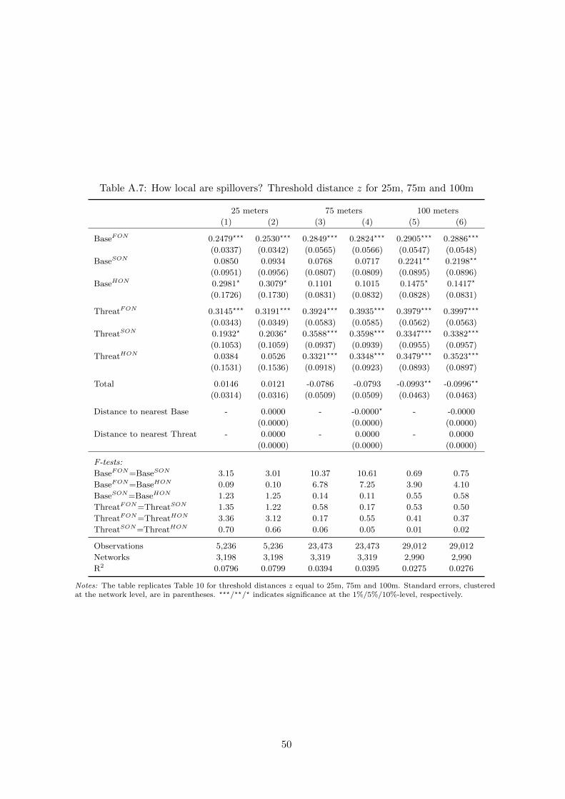
Table A.7: How local are spillovers? Threshold distance z for 25m, 75m and 100m
25 meters 75 meters 100 meters
(1) (2) (3) (4) (5) (6)
BaseFON 0.2479??? 0.2530??? 0.2849??? 0.2824??? 0.2905??? 0.2886???
(0.0337) (0.0342) (0.0565) (0.0566) (0.0547) (0.0548)
BaseSON 0.0850 0.0934 0.0768 0.0717 0.2241?? 0.2198??
(0.0951) (0.0956) (0.0807) (0.0809) (0.0895) (0.0896)
BaseHON 0.2981? 0.3079? 0.1101 0.1015 0.1475? 0.1417?
(0.1726) (0.1730) (0.0831) (0.0832) (0.0828) (0.0831)
ThreatFON 0.3145??? 0.3191??? 0.3924??? 0.3935??? 0.3979??? 0.3997???
(0.0343) (0.0349) (0.0583) (0.0585) (0.0562) (0.0563)
ThreatSON 0.1932? 0.2036? 0.3588??? 0.3598??? 0.3347??? 0.3382???
(0.1053) (0.1059) (0.0937) (0.0939) (0.0955) (0.0957)
ThreatHON 0.0384 0.0526 0.3321??? 0.3348??? 0.3479??? 0.3523???
(0.1531) (0.1536) (0.0918) (0.0923) (0.0893) (0.0897)
Total 0.0146 0.0121 -0.0786 -0.0793 -0.0993?? -0.0996??
(0.0314) (0.0316) (0.0509) (0.0509) (0.0463) (0.0463)
Distance to nearest Base - 0.0000 - -0.0000? - -0.0000
(0.0000) (0.0000) (0.0000)
Distance to nearest Threat - 0.0000 - 0.0000 - 0.0000
(0.0000) (0.0000) (0.0000)
F-tests:
BaseFON=BaseSON 3.15 3.01 10.37 10.61 0.69 0.75
BaseFON=BaseHON 0.09 0.10 6.78 7.25 3.90 4.10
BaseSON=BaseHON 1.23 1.25 0.14 0.11 0.55 0.58
ThreatFON=ThreatSON 1.35 1.22 0.58 0.17 0.53 0.50
ThreatFON=ThreatHON 3.36 3.12 0.17 0.55 0.41 0.37
ThreatSON=ThreatHON 0.70 0.66 0.06 0.05 0.01 0.02
Observations 5,236 5,236 23,473 23,473 29,012 29,012
Networks 3,198 3,198 3,319 3,319 2,990 2,990
R2 0.0796 0.0799 0.0394 0.0395 0.0275 0.0276
Notes: The table replicates Table 10 for threshold distances z equal to 25m, 75m and 100m. Standard errors, clusteredat the network level, are in parentheses. ???/??/? indicates significance at the 1%/5%/10%-level, respectively.
50

Appendix B Theoretical Background
In this section we provide more background on the theoretical model from Section 6. We first
highlight how our basic estimation equation (1) can be understood in terms of the consensus be-
lief p∗ (section Appendix B.1). We then discuss the different network characteristics (Appendix
B.2) and local concentration measures in more detail (Appendix B.3). Finally we discuss how
local we should expect spillovers to be (Appendix B.4).
Appendix B.1 Long Run Consensus
Remember the updating process described in Section 6, equation (2). DeGroot (1974) and
DeMarzo et al. (2003) have shown that, under mild conditions on the network structure, updating
processes as the one described in equation (2) converge to a consensus propensity p∗i = p∗, ∀i ∈ Nwhich is shared by all agents in the network. The consensus propensity will be a weighted average
of all households pre-communication propensity p0, i.e.,
p∗ =∑j∈N
ωjp0j , (B.1)
where the weights ωj are determined by (i) the initial weights λij in updating rule (2), and (ii)
the network position of household j and all other households.
Can our estimation equation from (1) be understood in terms of the long-run consensus
described in equation (B.1)? To answer this question, let us focus on untreated non-compliant
households (type II). We are interested in understanding their compliance decision
yi =
{1 if p∗i ≥ pi0 else
(B.2)
If we assume that households of the same category τ ∈ {a, b, c, d} share the same prior, then we
can rewrite equation (B.1) as follows
p∗i =∑
j 6=i:τ(j)=a
ωjp0a
N+
∑j 6=i:τ(j)=b
ωjp0b
N+
∑j 6=i:τ(j)=c
ωjp0c
N+
∑j 6=i:τ(j)=d
ωjp0d
N, (B.3)
where p0τ , τ = a, b, c, d is the prior of households in category τ and τ(j) is the category household
j falls into. This can be rewritten as
p∗i = ωap0a
∑j 6=i:τj=a
N+ ωbp
0b
∑j 6=i:τj=b
N+ ωcp
0c
∑j 6=i:τj=c
N+ ωdp
0d(1−
∑j 6=i:τj∈{a,b,c}
N), (B.4)
where ωτ =∑
j 6=i:τ(j)=τ ωj . The coefficients from our basic estimation equation from Section 5,
yi = α+ β0Total + β1Base+ β2Threat+ εi,
with Threat =∑a
N−1 , Base =∑b
N−1 and Total =∑a,b,c
N−1 , then reflect a joint effect of the weights
and pre-communication propensities of the different categories of households. Note that the
theoretical model uses rates defined over N . However, these rates would not be suitable for our
empirical analysis (as pointed out above, e.g., in footnote 16). To see this, recall that we model
the decision of an untreated, non-compliant households i. As such a type II household is never
51

treated by definition, treatment-ratios defined over the full network size N (rather than N − 1)
would vary between 0 andN−1N . Hence, these alternative rates would be mechanically correlated
with the network size. We avoid this problem by using variables that capture the treatment
rates among other households, i.e., we use N − 1 as a denominator.
If one is willing to make further assumptions on the weights λij that households place on their
neighbors’ (and their own) propensities in the communication process, then more can be said
about the weights ω in the long run consensus. For example, if we assume that λij = λj ,∀i, j,i.e., if all households i (who are neighbors of j) place the same weight on j, then ωi
ωj=
λi∑h∈Ni
λh
λj∑h∈Nj
λh.
If weights are symmetric, i.e., if λij = λji,∀i, j, then ωiωj
=
∑h∈Ni
λhi∑h∈Nj
λhj. Finally, if all weights are
equal, i.e., if λij = λ,∀i, j, then ωiωj
= cardNicardNj , where cardNi measures household i’s degree, i.e.,
the number of her FONs. These results can be found in Theorem 7 in DeMarzo et al. (2003). In
the latter case, for example, we could interpret the ratio β1β2
as a product of the relative degree of
base- and threat- treated households in the network multiplied by the relative strength of priorsp0bp0c
. Since the degrees can be observed and the ratio of pre-communication beliefs inferred from
direct effects, making such assumptions would allow identification of λ.
Appendix B.2 Network Characteristics
This section defines and explains the network characteristics referred to in Section 6. Recall
that we refer to A = [aij] as the adjacency matrix of a network, where aij = 1 if there is a link
between households i and j (i.e., if (i, j) ∈ Ξ) and zero otherwise.
(i) Degree. The degree of household i is given by the number of its first-order neighbors
(FONs), i.e., by the cardinality of the set Ni.
(ii) Clustering. The clustering coefficient is the fraction of neighbors of i who are neighbors
themselves. The clustering coefficient ci of household i is defined as follows:
ci =
∑j<k aijaikajk∑j<k aijaik
.
(iii) Eigenvector Centrality. Eigenvector centrality (EC) is one of several measures that
determine the relative importance of a node within a network. The measure assigns rel-
ative scores to all nodes in the network, assuming that connections to high-scoring nodes
contribute more to the score of the node in question than equal connections to low-scoring
nodes. Eigenvector centrality is defined as
ECi =1
λ
∑j∈Ni
ECj =1
λ
∑j∈N
aijECj .
The equality can be rewritten as the eigenvector equation AEC = λEC. Newman (2006)
shows that only the highest λ satisfies the requirement of entirely positive entries of the
vector EC and thus, eigenvector centrality of agent i is uniquely determined as the ith
entry of the respective eigenvector EC.
How should these characteristics affect spillovers? In the main text we have argued that
eigenvector centrality is of particular relevance in determining the weights of households in the
52

long run consensus and hence the size of spillovers. To see this, recall from equation (4) and
our discussion in Section 6.1 that the weights of agents in the final consensus can be expressed
by solving the row eigenvector equation ωT = ω. Since T can be interpreted as the transition
matrix of a finite, irreducible, and aperiodic Markov chain, it has a unique eigenvalue equal to
one and all other eigenvalues with modulus smaller than one. The row eigenvector corresponding
to the largest eigenvalue coincides with the vector of weights ω = (ω1, ..., ωN ). This implies that
an agent’s weight in the final consensus ωi is closely related to her eigenvector centrality. In the
special case where λij = λ, ∀i, j (see Appendix B.1), an agent’s weight in ωi exactly coincides
with her eigenvector centrality.
Appendix B.3 Local Concentration of Intervention
We use three different measures of local concentration. To define these measures, we need to
introduce some notation. Define by inτk the average number of neighbors of type-τ agents in
network k, who are also of type τ . Define by outτk the average number of neighbors of type-τ
agents in network k, who are not of type τ . (Obviously, inτk + outτk coincides with the average
degree of type-τ households in network k, i.e., with their average number of FONs.) We can
then define the index Hτk =
inτkinτk+outτk
(compare Currarini et al., 2009). Based on this, we can
now introduce:
(i) LC Dummy: LCDτk equals one if there are at least two households who received a given
mailing treatment (baseline or threat) and are also FONs, i.e., if inτk > 0.
(ii) IH-Index: The inbreeding homophily index for type τ is given by IHτk =
Hτk−
N−1N
(τ−ratek)
1−N−1N
(τ−ratek).
(iii) IH Dummy: IHDτk = 1↔ IHτ
k ≥ 0.
The IH-Index is positive if there is homophily and negative if there is heterophily. Note
that in small networks the IH-index is slightly biased downwards in the sense that in the case of
purely random linking, the expected value of the index would be −1N−1 . This expression converges
to zero as N becomes large, but it is clearly different from zero (and negative) for small network
sizes. The latter fact motivates us to consider the IH Dummy, which indicates simply whether
there is homophily in the network or not.
Golub and Jackson (2012) have asked whether local concentration helps or hinders conver-
gence in the deGroot model (DeGroot, 1974). They find that local concentration is detrimental
(Theorem 1 in Golub and Jackson, 2012). Several differences between the assumptions underly-
ing their result and our empirical approach should be noted. First, they use a spectral measure
of homophily while we work with the inbreeding-homophily index. The latter is more common in
empirical work (e.g., Currarini et al., 2009). Second, they need a number of assumptions to show
their result. One of these (‘comparable densities’) requires that the interaction probabilities of
different types do not diverge. We cannot ensure this, since in some of our networks some types
do not occur (if, e.g., no one was treated with a baseline-letter).
Appendix B.4 How local are spillovers?
Let us now derive some comparative statics for cases where communication ends before a con-
sensus is reached. We have assumed that in each round r agents update their beliefs according
53

to equation (2). After one round of communication, household i’s compliance propensity is then
given by
p1i =
∑j∈Ni λij p
0j + λii p
0i∑
j∈Ni λij + λii, (B.5)
Hence, after one round of communication, the marginal effect from a treated household `’s
propensity on the propensity of her FON i is given by
∂p1i
∂p0`
=λi`∑
j∈Ni λij + λii. (B.6)
After two rounds of communication, i’s beliefs will have the following shape:
p2i =
∑j∈Ni
λij∑j∈Ni λij + λii
(∑`∈Nj λj` p
0` + λjj p
0j∑
`∈Nj λj` + λjj
)
+λii∑
j∈Ni λij + λii
(∑j∈Ni λij p
rj + λii p
ri∑
j∈Ni λij + λii
). (B.7)
After two rounds of communication, the marginal effect of increasing the treated household k’s
propensity on the propensity of her SON i is thus given by
∂p2i
∂p0k
=
∑j∈(Ni∩Nk) λij
λjk∑h∈Nj
λjh+λjj∑j∈Ni λij + λii
. (B.8)
This derivative is composed of two effects: first, the weight that household i places on those
FONs who are also linked to the targeted node k (the agents in Ni∩Nk) and, second, the weight
that these FONs place on k. Hence the size of the effect will depend on how many agents j
connect i to k (indirectly) and how much weight these agents place on k. Since
∑j∈(Ni∩Nk)
λij∑j∈Ni
λij+λii< 1,
it follows that – as long as λij = λik, ∀j, k 6= i, i.e., as long as agents place the same weight on
all their neighbors – the marginal effect on any given SON is smaller than the marginal effect on
FONs. The probability that a non-treated household starts to comply should therefore be higher
if it is a FON of a treated household compared to when it is a SON of a treated household.43
By the same logic, the probability that a SON of a treated household starts to comply should
cet. par. be higher than the probability that a third-order neighbor switches to compliance, etc.
43Note that while the marginal effect on any given FONs is always higher than that on a SON, this does notnecessarily mean that the spillover among FONs is higher. This will depend on how many FONs and SONsneighbors the treated household has. This again supports estimating a model in rates, such as in equation (1).
54


![Learning Query-Dependent Distance Metrics for Interactive ...staff.computing.dundee.ac.uk/stephen/PreprintICVS09.pdf · tures. Hu et al. [5] explored a multiple-instance ranking approach](https://img.pdfslide.net/doc/110x75/6016ca3f33ffae416013606d/learning-query-dependent-distance-metrics-for-interactive-staff-tures-hu-et.jpg)