Embed Size (px)
Citation preview
Working Paper Series
ISSN 1518-3548
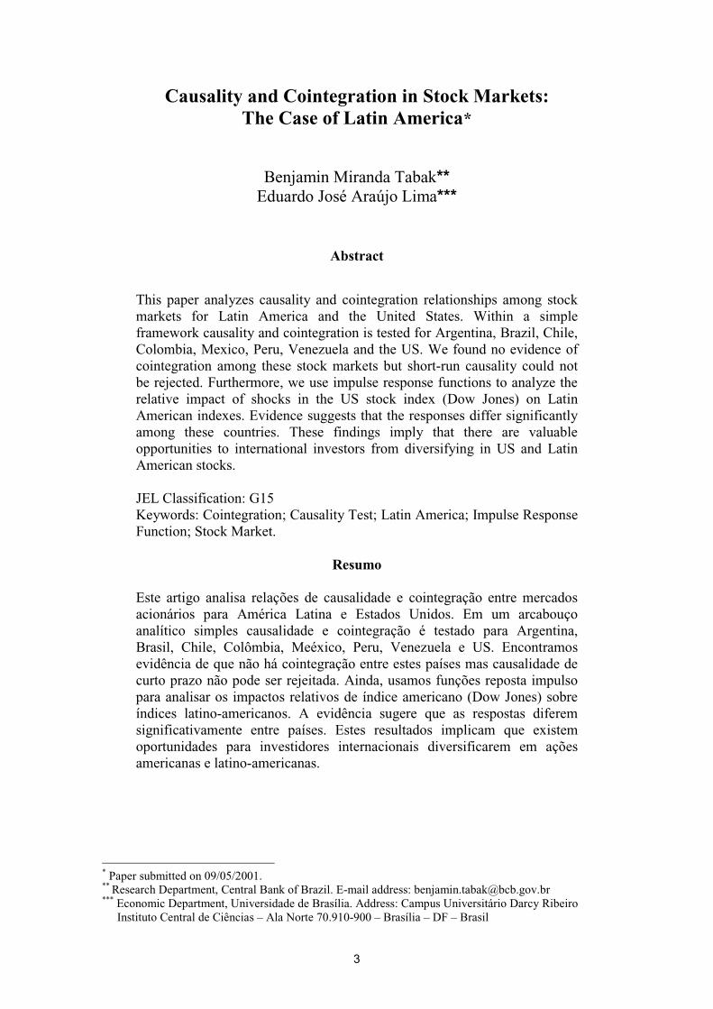
Causality and Cointegration in Stock Markets:the Case of Latin America
Benjamin Miranda Tabak and Eduardo José Araújo LimaDecember, 2002

ISSN 1518-3548 CGC 00.038.166/0001-05
Working Paper Series
Brasília
n. 56
Dec
2002
P. 1-28

Working Paper Series
Edited by: Research Department (Depep)
(E-mail: [email protected])
Reproduction permitted only if source is stated as follows: Working Paper Series n. 56 Authorized by Ilan Goldfajn (Deputy Governor for Economic Policy). General Control of Subscription: Banco Central do Brasil
Demap/Disud/Subip
SBS – Quadra 3 – Bloco B – Edifício-Sede – 2º subsolo
70074-900 Brasília – DF – Brazil
Phone: (5561) 414-1392
Fax: (5561) 414-3165
The views expressed in this work are those of the authors and do not reflect those of the Banco Central or its members. Although these Working Papers often represent preliminary work, citation of source is required when used or reproduced. As opiniões expressas neste trabalho são exclusivamente do(s) autor(es) e não refletem a visão do Banco Central do Brasil. Ainda que este artigo represente trabalho preliminar, citação da fonte é requerida mesmo quando reproduzido parcialmente. Banco Central do Brasil Information Bureau Address: Secre/Surel/Diate
SBS – Quadra 3 – Bloco B
Edifício-Sede – 2º subsolo
70074-900 Brasília – DF – Brazil
Phones: (5561) 414 (....) 2401, 2402, 2403, 2404, 2405, 2406
DDG: 0800 992345
Fax: (5561) 321-9453
Internet: http://www.bcb.gov.br
E-mails: [email protected]
3
Causality and Cointegration in Stock Markets: The Case of Latin America*
Benjamin Miranda Tabak** Eduardo José Araújo Lima***
Abstract
This paper analyzes causality and cointegration relationships among stock markets for Latin America and the United States. Within a simple framework causality and cointegration is tested for Argentina, Brazil, Chile, Colombia, Mexico, Peru, Venezuela and the US. We found no evidence of cointegration among these stock markets but short-run causality could not be rejected. Furthermore, we use impulse response functions to analyze the relative impact of shocks in the US stock index (Dow Jones) on Latin American indexes. Evidence suggests that the responses differ significantly among these countries. These findings imply that there are valuable opportunities to international investors from diversifying in US and Latin American stocks. JEL Classification: G15 Keywords: Cointegration; Causality Test; Latin America; Impulse Response Function; Stock Market.
Resumo Este artigo analisa relações de causalidade e cointegração entre mercados acionários para América Latina e Estados Unidos. Em um arcabouço analítico simples causalidade e cointegração é testado para Argentina, Brasil, Chile, Colômbia, Meéxico, Peru, Venezuela e US. Encontramos evidência de que não há cointegração entre estes países mas causalidade de curto prazo não pode ser rejeitada. Ainda, usamos funções reposta impulso para analisar os impactos relativos de índice americano (Dow Jones) sobre índices latino-americanos. A evidência sugere que as respostas diferem significativamente entre países. Estes resultados implicam que existem oportunidades para investidores internacionais diversificarem em ações americanas e latino-americanas.
* Paper submitted on 09/05/2001. ** Research Department, Central Bank of Brazil. E-mail address: [email protected] *** Economic Department, Universidade de Brasília. Address: Campus Universitário Darcy Ribeiro Instituto Central de Ciências – Ala Norte 70.910-900 – Brasília – DF – Brasil
4
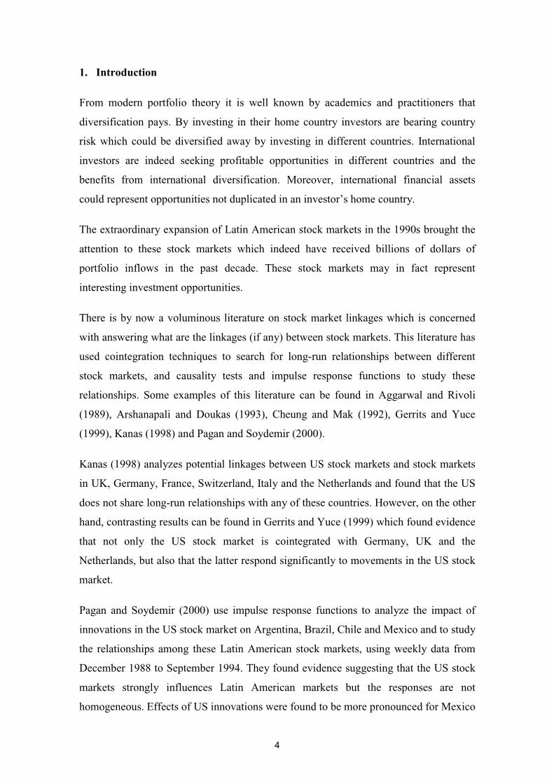
1. Introduction
From modern portfolio theory it is well known by academics and practitioners that
diversification pays. By investing in their home country investors are bearing country
risk which could be diversified away by investing in different countries. International
investors are indeed seeking profitable opportunities in different countries and the
benefits from international diversification. Moreover, international financial assets
could represent opportunities not duplicated in an investor’s home country.
The extraordinary expansion of Latin American stock markets in the 1990s brought the
attention to these stock markets which indeed have received billions of dollars of
portfolio inflows in the past decade. These stock markets may in fact represent
interesting investment opportunities.
There is by now a voluminous literature on stock market linkages which is concerned
with answering what are the linkages (if any) between stock markets. This literature has
used cointegration techniques to search for long-run relationships between different
stock markets, and causality tests and impulse response functions to study these
relationships. Some examples of this literature can be found in Aggarwal and Rivoli
(1989), Arshanapali and Doukas (1993), Cheung and Mak (1992), Gerrits and Yuce
(1999), Kanas (1998) and Pagan and Soydemir (2000).
Kanas (1998) analyzes potential linkages between US stock markets and stock markets
in UK, Germany, France, Switzerland, Italy and the Netherlands and found that the US
does not share long-run relationships with any of these countries. However, on the other
hand, contrasting results can be found in Gerrits and Yuce (1999) which found evidence
that not only the US stock market is cointegrated with Germany, UK and the
Netherlands, but also that the latter respond significantly to movements in the US stock
market.
Pagan and Soydemir (2000) use impulse response functions to analyze the impact of
innovations in the US stock market on Argentina, Brazil, Chile and Mexico and to study
the relationships among these Latin American stock markets, using weekly data from
December 1988 to September 1994. They found evidence suggesting that the US stock
markets strongly influences Latin American markets but the responses are not
homogeneous. Effects of US innovations were found to be more pronounced for Mexico
5
than for Argentina, Chile or Brazil. Finally, Argentina and Chile seemed to be more
responsive to a Brazilian market shock than to a shock originating from Mexico1.
The objective of this paper is to provide further evidence on the linkages between Latin
American equity markets and the US equity market. We focus on Argentina, Brazil,
Chile, Colombia, Peru, Mexico and Venezuela and the US extending the number of
countries which are usually used in studies of equity market integration.
Using the Johansen methodology, we search for a pairwise cointegration among Latin
American stock markets and the US. Granger causality tests were used to study the
interrelationships between these stock markets. We also test for short-run causality
between Latin American stock markets, focusing on how these stock markets respond to
shocks in the US stock market, using impulse response functions. We extend Pagan and
Soydemir’s (2000) study analyzing impulse response functions using daily data from
January 1995 to March 2001.
Our findings suggest that Latin American equity markets are not cointegrated with the
US equity market. However, shocks in the US equity stock market affect Latin
American stock markets. Additionally, Latin American equity markets seem to respond
differently to shocks in the US stock markets. Finally impulse response functions show
evidence that Latin American equity markets respond more quickly for the current
period than for the period covered by Pagan and Soydemir (2001). These findings are
valuable to investors evaluating international portfolios.
The remainder of the paper is structured as follows. In the next section we present the
data used in this study. Section 3 covers the methodology employed, while Section 4
shows the empirical evidence. Section 5 concludes the paper.
1 The authors argue that results may be attributed to tighter trading relations between US and Mexico, and Argentina and Chile with Brazil.
6
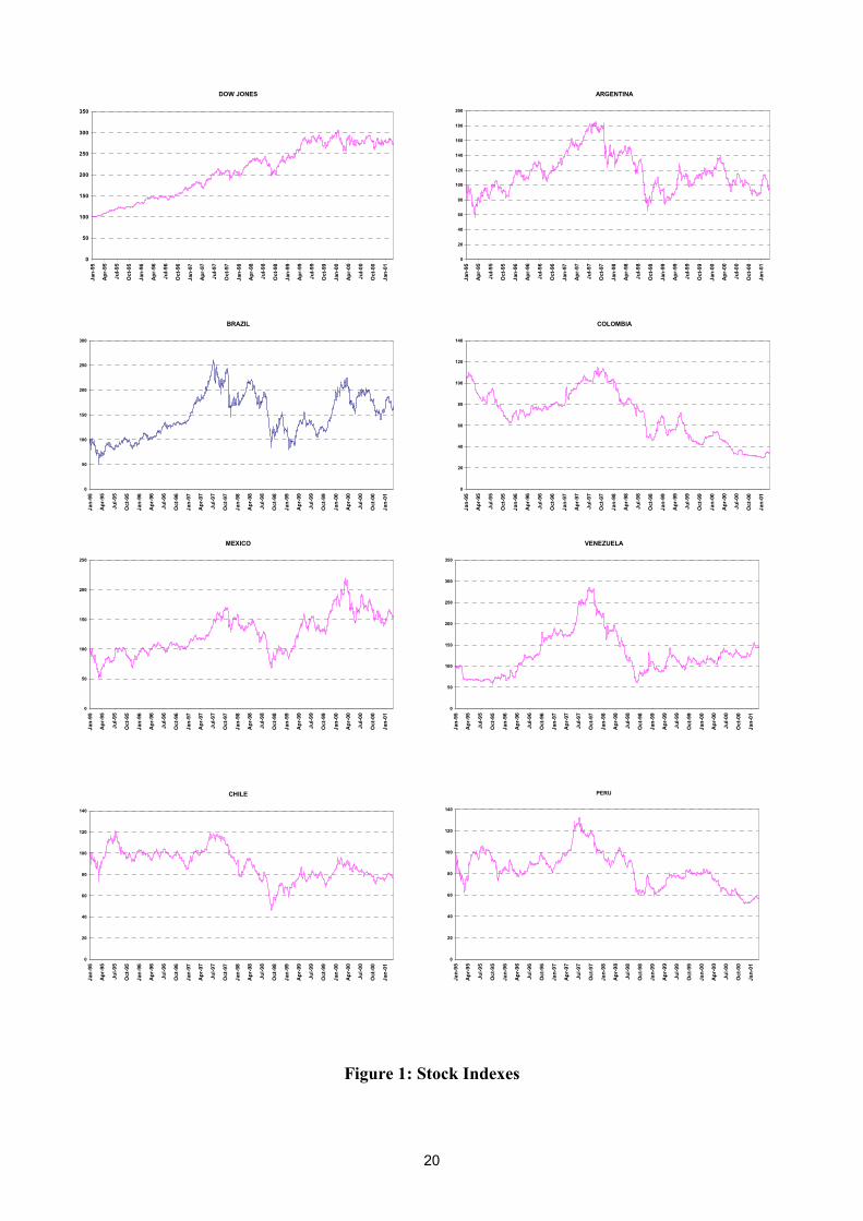
2. The Data
The data set used in this study comprise daily close quotes for stock prices. We use (1)
the Dow Jones Industrial Average (US), (2) the MERVAL from Argentina, (3) the
IBOVESPA (Indice da Bolsa de Valores de São Paulo) from Brazil, (4) the IBB (Indice
de la Bolsa de Bogota) from Colombia, (5) the IGPA (Indice General de Precios de
Acciones) from Chile, (6) the IPC (Indice de Precios y Cotizaciones) from Mexico, (7)
the IBC (Indice de la Bolsa de Caracas) from Venezuela, and (8) the IGBVL (Indice
General de la Bolsa de Valores de Lima) from Peru. The daily indices were obtained
from the Economatica database.
The Dow Jones Industrial Average is a price-weighted average of 30 blue chip stocks
that are generally the leaders in their industry. The IBOVESPA is an equity index
weighted by traded volume and is comprised of the most liquid stocks traded in the São
Paulo Stock Exchange. The MERVAL Index is the market value of a stock portfolio,
selected according to participation in the Buenos Aires Stock Exchange. The IPC is a
capitalization-weighted index of the leading stocks traded on the Mexico Stock
Exchange. The IGPA is a capitalization-weighted index of the majority of the
companies traded on the Santiago Stock Exchange. The IBB is an index composed of
shares from 20 companies whose volume has been the highest in the past 2 years. The
IBC is a capitalization-weighted index of the 15 most liquid and highest capitalized
stocks traded on the Caracas Stock Exchange. The IGBVL is an index composed of
shares from 29 companies which are the most actively traded in the Peruvian stock
market. Therefore, these indexes can be seen as their countries stock markets
benchmarks.
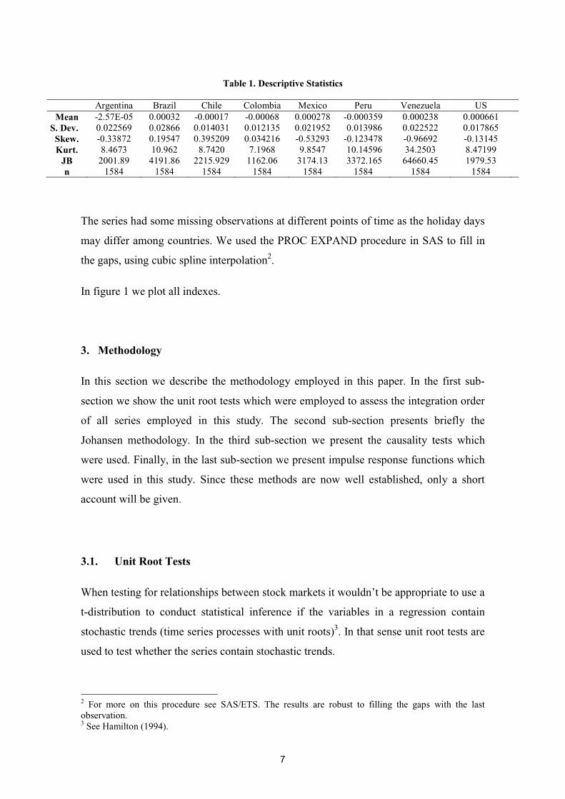
The data begins in January 3 1995 and ends in March 1 2001. All series are in US
dollars. In table 1 descriptive statistics for returns on these stock indexes are shown. As
we can see only Chile, Colombia and Peru have standard deviations lower than the Dow
Jones. Normality is rejected for all series as the Jarque-Bera (JB) statistics shown in
table 1 are quite large.
7
Table 1. Descriptive Statistics
Argentina Brazil Chile Colombia Mexico Peru Venezuela US Mean -2.57E-05 0.00032 -0.00017 -0.00068 0.000278 -0.000359 0.000238 0.000661
S. Dev. 0.022569 0.02866 0.014031 0.012135 0.021952 0.013986 0.022522 0.017865 Skew. -0.33872 0.19547 0.395209 0.034216 -0.53293 -0.123478 -0.96692 -0.13145 Kurt. 8.4673 10.962 8.7420 7.1968 9.8547 10.14596 34.2503 8.47199
JB 2001.89 4191.86 2215.929 1162.06 3174.13 3372.165 64660.45 1979.53 n 1584 1584 1584 1584 1584 1584 1584 1584
The series had some missing observations at different points of time as the holiday days
may differ among countries. We used the PROC EXPAND procedure in SAS to fill in
the gaps, using cubic spline interpolation2.
In figure 1 we plot all indexes.
3. Methodology
In this section we describe the methodology employed in this paper. In the first sub-
section we show the unit root tests which were employed to assess the integration order
of all series employed in this study. The second sub-section presents briefly the
Johansen methodology. In the third sub-section we present the causality tests which
were used. Finally, in the last sub-section we present impulse response functions which
were used in this study. Since these methods are now well established, only a short
account will be given.
3.1. Unit Root Tests
When testing for relationships between stock markets it wouldn’t be appropriate to use a
t-distribution to conduct statistical inference if the variables in a regression contain
stochastic trends (time series processes with unit roots)3. In that sense unit root tests are
used to test whether the series contain stochastic trends.
2 For more on this procedure see SAS/ETS. The results are robust to filling the gaps with the last observation. 3 See Hamilton (1994).
8
In order to assess if the indexes have unit roots a widely accepted test is the Augmented
Dickey and Fuller (1979) test. Let Xt be a time series. The ADF test involves estimating
the equation below:
( ) tit
k
iitt XXtX εϕρβα +∆+−++=∆ −
−
=− ∑
1
111 (1)
and testing whether 1=ρ . In this equation L−=∆ 1 (where L is a lag operator); t is a
trend; and tε is a white noise term. Phillips and Perron (1988) tests were also conducted,
which allow for more general error terms (heteroskedastic and autocorrelated errors).
3.2. Cointegrating tests
Let’s consider a VAR of order p, where Xt is a p-vector of I(1) variables and εt is a
vector of innovations, as given in equation (2).
tptptt XAXAX ε+⋅⋅⋅+= −−11 (2)
We can rewrite this expression as:
tjtj
p
jtt XXX ε+∆Γ+Π=∆ −
−
=− ∑
1
11
(3)
where
IAp
jj −=Π ∑
=1 and ∑
+=
−=Γp
jiij A
1 (4)
If the coefficient matrix Π has reduced rank r < p, then there exist p x r matrices and α
and β such that Π = αβ’, and β’Xt is stationary, i.e., the hypothesis of cointegration is
formulated as a restriction on the matrix Π where the number of cointegrating relations
9
is given by r. Johansen’s method involves estimating the Π matrix in an unrestricted
form and then testing whether the restrictions implied by the reduced rank of Π can be
rejected4.
We test for r (the maximum number of cointegrating relationships) using the λtrace
statistic, where
( )∑+=
−−=p
riit n
1race
ˆ1ln λλ (5)
where iλ̂ is the i-th largest eigenvalue λtrace is a test of the null of r cointegrating rank
against the alternative of a p cointegrating rank.
We also use the maximum eigenvalue statistic (λmax). We use this statistic to improve
the power of the test by limiting the alternative to a cointegrating rank just one more
than under the null. This statistic is given by:
( )in λλ ˆ1lnmax −−= (6)
where this statistics tests the null of rank equal to r against the alternative of r+1.
3.3. Causality Tests
To test whether there are contagion effects (short-run causality) within stock market
indexes we use the following vector auto-regression (see Granger (1969)):
t
k
iiti
k
iitit xxx 1
122
11101 εααα +∆+∆+=∆ ∑∑
=−
=−
(7)
t
k
iiti
k
iitit xxx 2
122
11102 εβββ +∆+∆+=∆ ∑∑
=−
=−
(8)
4 Cointegration theory implies that for a vector of time series, the variables are said to be cointegrated if linear combinations are stationary without differencing, even if the individual elements of the vector need to be differenced at least once to become stationary. The reader is referred to Johansen (1988, 1990) and Johansen and Juselius (1990) for a complete description of the estimation technique.
10
where ∆ is the first difference operator and we have assumed that X1 and X2 are not
cointegrated. If the α2i are statistically different from zero for different lags then we can
reject the absence of granger causality and we can say that X2 granger causes X1. If the
β1i are statistically significant the direction of causality is from X1 to X2. If both are
different from zero then we can say that there exists bicausality.
If they are cointegrated these equations would need an additional error correction term,
and the appropriate test would be given by
( ) t
k
iiti
k
iitittt xxxxx 1
122
1111211101 εααγδα +∆+∆+−+=∆ ∑∑
=−
=−−−
(9)
( ) t
k
iiti
k
iitittt xxxxx 2
122
1111211202 εββγδβ +∆+∆+−+=∆ ∑∑
=−
=−−−
(10)
The term ( )1211 −− − tt xx γ is an error correction term determined from the level form
estimate of the long-run relationship between X1 and X2. Causality now can be asserted
by the significance of the parameters α2i , β1i , δ1 and δ2. If δ1 is significantly different
from zero but δ2 is not then if X1 and X2 drift apart the X1 variables will correct to
restore equilibrium. If δ1 is not significantly different from zero δ2 but δ1 is then X2
makes the correction. If both δ1 and δ2 are significant then both X1 and X2 will have a
correction to restore equilibrium5.
3.4. Impulse response functions
In order to analyze the effects of shocks in one stock market into the other we use a well
known technique in the literature which is called impulse response functions.
A VAR can be written in a vector MA(∞) such as
⋅⋅⋅+Ψ+Ψ+Ψ++= −−− 332211 ttttty εεεεµ (11)
In this case the matrix Ψ has the following interpretation:
t
sts
y
ε∂∂=Ψ + (12)
11
The row i, column j, of Ψs identifies the consequences of a one-unit increase in the jth
variable’s innovation at date t, holding all other innovations constant6. These are called
impulse response functions (IRF). We can use these IRF to analyze the impact of shocks
in the US stock market on Latin American stock market indexes. This will be done in
the next section.
4. Empirical Results
In this section we present the empirical results found for the data set employed in this
study. Sub-section 4.1 presents unit root test results while sub-section 4.2. cointegration
tests. Sub-section 4.3 presents Granger causality tests and finally in sub-section 4.4
impulse response functions are analyzed.
4.1. Unit root tests results
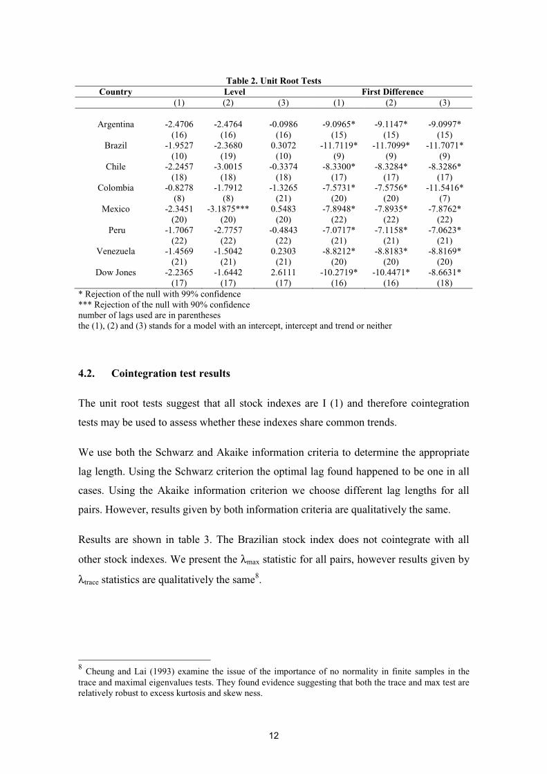
In table 2 results for unit root tests are presented. As it can be seen, for all variables one
cannot reject the null of integration of order 1. The unit root hypothesis cannot be
rejected in levels but it is rejected at the 99% level of confidence with first differences,
which suggests that these stock indexes are I(1) and not I(2).
The number of lags in the ADF tests was chosen running regression (1) with 22 lags of
the dependent variable. Then we checked whether this lag was significant, if it wasn’t
significant we reduced by 1 the number of lags and repeated this procedure until either a
statistically significant lag was found or there were no lags at all (conventional Dickey
and Fuller test)7.
5 See Engle and Granger (1987). 6 For more on these impulse response functions the reader is referred to Hamilton (1994). 7 In the interest of space, Phillips and Perron (1988) unit root tests are not reported. However, these unit root tests yield qualitatively identical results.
12
Table 2. Unit Root Tests
Country Level First Difference (1) (2) (3) (1) (2) (3)
Argentina -2.4706 (16)
-2.4764 (16)
-0.0986 (16)
-9.0965* (15)
-9.1147* (15)
-9.0997* (15)
Brazil -1.9527 (10)
-2.3680 (19)
0.3072 (10)
-11.7119* (9)
-11.7099* (9)
-11.7071* (9)
Chile -2.2457 (18)
-3.0015 (18)
-0.3374 (18)
-8.3300* (17)
-8.3284* (17)
-8.3286* (17)
Colombia -0.8278 (8)
-1.7912 (8)
-1.3265 (21)
-7.5731* (20)
-7.5756* (20)
-11.5416* (7)
Mexico -2.3451 (20)
-3.1875*** (20)
0.5483 (20)
-7.8948* (22)
-7.8935* (22)
-7.8762* (22)
Peru -1.7067 (22)
-2.7757 (22)
-0.4843 (22)
-7.0717* (21)
-7.1158* (21)
-7.0623* (21)
Venezuela -1.4569 (21)
-1.5042 (21)
0.2303 (21)
-8.8212* (20)
-8.8183* (20)
-8.8169* (20)
Dow Jones -2.2365 (17)
-1.6442 (17)
2.6111 (17)
-10.2719* (16)
-10.4471* (16)
-8.6631* (18)
* Rejection of the null with 99% confidence *** Rejection of the null with 90% confidence number of lags used are in parentheses the (1), (2) and (3) stands for a model with an intercept, intercept and trend or neither
4.2. Cointegration test results
The unit root tests suggest that all stock indexes are I (1) and therefore cointegration
tests may be used to assess whether these indexes share common trends.
We use both the Schwarz and Akaike information criteria to determine the appropriate
lag length. Using the Schwarz criterion the optimal lag found happened to be one in all
cases. Using the Akaike information criterion we choose different lag lengths for all
pairs. However, results given by both information criteria are qualitatively the same.
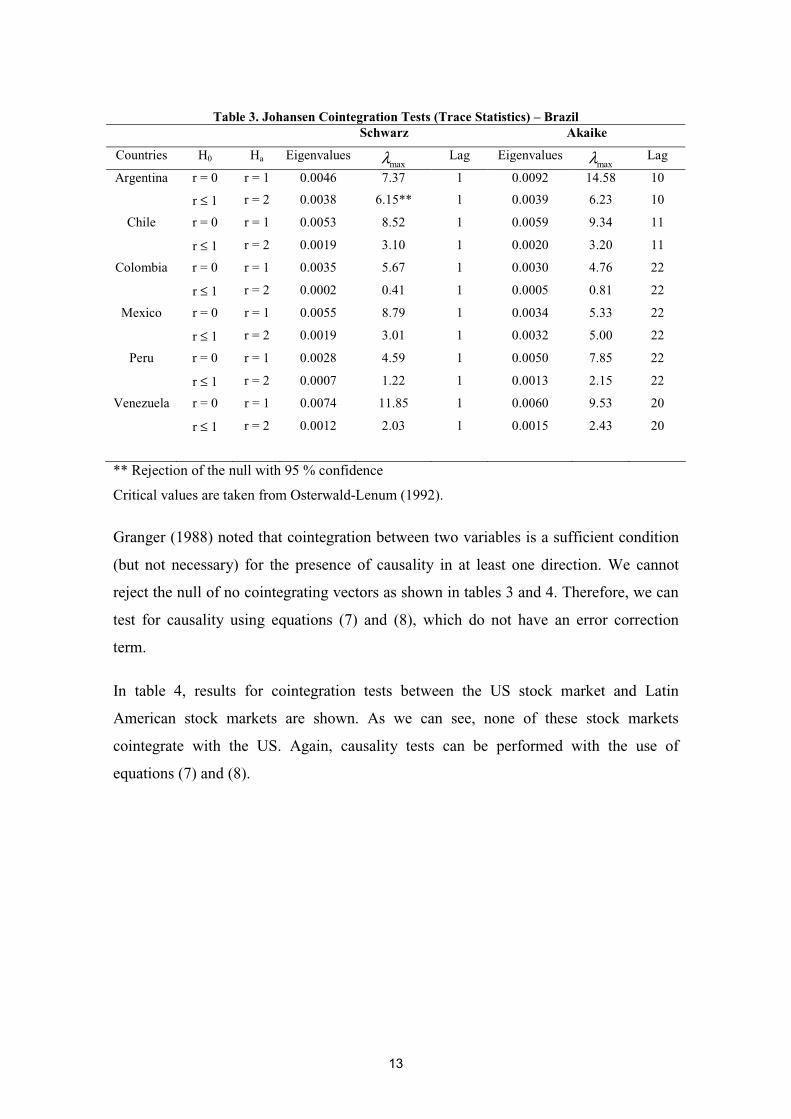
Results are shown in table 3. The Brazilian stock index does not cointegrate with all
other stock indexes. We present the λmax statistic for all pairs, however results given by
λtrace statistics are qualitatively the same8.
8 Cheung and Lai (1993) examine the issue of the importance of no normality in finite samples in the trace and maximal eigenvalues tests. They found evidence suggesting that both the trace and max test are relatively robust to excess kurtosis and skew ness.
13
Table 3. Johansen Cointegration Tests (Trace Statistics) – Brazil
Schwarz Akaike
Countries H0 Ha Eigenvaluesmaxλ Lag Eigenvalues
maxλ Lag
Argentina r = 0 r = 1 0.0046 7.37 1 0.0092 14.58 10
r ≤ 1 r = 2 0.0038 6.15** 1 0.0039 6.23 10
Chile r = 0 r = 1 0.0053 8.52 1 0.0059 9.34 11
r ≤ 1 r = 2 0.0019 3.10 1 0.0020 3.20 11
Colombia r = 0 r = 1 0.0035 5.67 1 0.0030 4.76 22
r ≤ 1 r = 2 0.0002 0.41 1 0.0005 0.81 22
Mexico r = 0 r = 1 0.0055 8.79 1 0.0034 5.33 22
r ≤ 1 r = 2 0.0019 3.01 1 0.0032 5.00 22
Peru r = 0 r = 1 0.0028 4.59 1 0.0050 7.85 22
r ≤ 1 r = 2 0.0007 1.22 1 0.0013 2.15 22
Venezuela r = 0 r = 1 0.0074 11.85 1 0.0060 9.53 20
r ≤ 1 r = 2 0.0012 2.03 1 0.0015 2.43 20
** Rejection of the null with 95 % confidence
Critical values are taken from Osterwald-Lenum (1992).
Granger (1988) noted that cointegration between two variables is a sufficient condition
(but not necessary) for the presence of causality in at least one direction. We cannot
reject the null of no cointegrating vectors as shown in tables 3 and 4. Therefore, we can
test for causality using equations (7) and (8), which do not have an error correction
term.
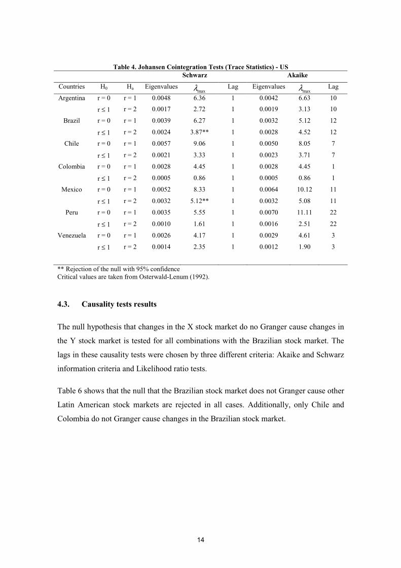
In table 4, results for cointegration tests between the US stock market and Latin
American stock markets are shown. As we can see, none of these stock markets
cointegrate with the US. Again, causality tests can be performed with the use of
equations (7) and (8).
14
Table 4. Johansen Cointegration Tests (Trace Statistics) - US Schwarz Akaike
Countries H0 Ha Eigenvaluesmaxλ Lag Eigenvalues
maxλ Lag
Argentina r = 0 r = 1 0.0048 6.36 1 0.0042 6.63 10
r ≤ 1 r = 2 0.0017 2.72 1 0.0019 3.13 10
Brazil r = 0 r = 1 0.0039 6.27 1 0.0032 5.12 12
r ≤ 1 r = 2 0.0024 3.87** 1 0.0028 4.52 12
Chile r = 0 r = 1 0.0057 9.06 1 0.0050 8.05 7
r ≤ 1 r = 2 0.0021 3.33 1 0.0023 3.71 7
Colombia r = 0 r = 1 0.0028 4.45 1 0.0028 4.45 1
r ≤ 1 r = 2 0.0005 0.86 1 0.0005 0.86 1
Mexico r = 0 r = 1 0.0052 8.33 1 0.0064 10.12 11
r ≤ 1 r = 2 0.0032 5.12** 1 0.0032 5.08 11
Peru r = 0 r = 1 0.0035 5.55 1 0.0070 11.11 22
r ≤ 1 r = 2 0.0010 1.61 1 0.0016 2.51 22
Venezuela r = 0 r = 1 0.0026 4.17 1 0.0029 4.61 3
r ≤ 1 r = 2 0.0014 2.35 1 0.0012 1.90 3
** Rejection of the null with 95% confidence Critical values are taken from Osterwald-Lenum (1992).
4.3. Causality tests results
The null hypothesis that changes in the X stock market do no Granger cause changes in
the Y stock market is tested for all combinations with the Brazilian stock market. The
lags in these causality tests were chosen by three different criteria: Akaike and Schwarz
information criteria and Likelihood ratio tests.
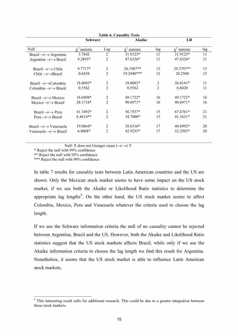
Table 6 shows that the null that the Brazilian stock market does not Granger cause other
Latin American stock markets are rejected in all cases. Additionally, only Chile and
Colombia do not Granger cause changes in the Brazilian stock market.
15
Table 6. Causality Tests
Schwarz Akaike LR
Null χ2 statistic Lag χ2 statistic lag χ2 statistic lag Brazil →/→ Argentina 3.7642 2 31.9123* 11 31.9123* 11 Argentina →/→ Brazil 9.2893* 2 47.6326* 11 47.6326* 11
Brazil →/→ Chile 9.7717* 2 26.1987** 12 29.3797** 15 Chile →/→Brazil 0.6438 2 19.2940*** 12 20.2580 15
Brazil →/→Colombia 18.0092* 2 18.0092* 2 36.0141* 11 Colombia →/→ Brazil 0.5562 2 0.5562 2 6.8420 11
Brazil →/→ Mexico 16.0498* 2 49.1722* 16 49.1722* 16 Mexico →/→ Brazil 28.1718* 2 90.6971* 16 90.6971* 16
Brazil →/→ Peru 41.3492* 2 56.7537* 15 67.6761* 21 Peru →/→ Brazil 6.4614** 2 34.7000* 15 41.1631* 21
Brazil →/→ Venezuela 19.0864* 2 38.6316* 17 40.6992* 20 Venezuela →/→ Brazil 6.8068* 2 42.9255* 17 52.2503* 20
Null: X does not Granger cause (→/→) Y * Reject the null with 99% confidence ** Reject the null with 95% confidence *** Reject the null with 90% confidence
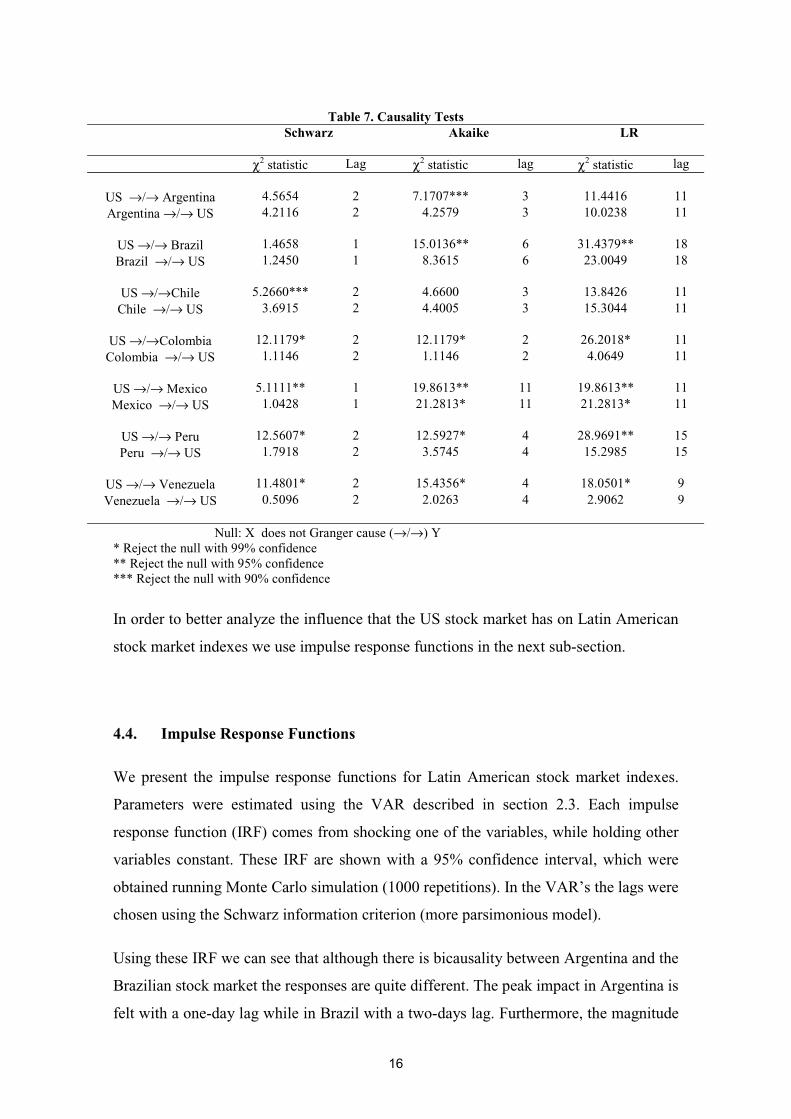
In table 7 results for causality tests between Latin American countries and the US are
shown. Only the Mexican stock market seems to have some impact on the US stock
market, if we use both the Akaike or Likelihood Ratio statistics to determine the
appropriate lag lengths9. On the other hand, the US stock market seems to affect
Colombia, Mexico, Peru and Venezuela whatever the criteria used to choose the lag
length.
If we use the Schwarz information criteria the null of no causality cannot be rejected
between Argentina, Brazil and the US. However, both the Akaike and Likelihood Ratio
statistics suggest that the US stock markets affects Brazil, while only if we use the
Akaike information criteria to choose the lag length we find this result for Argentina.
Nonetheless, it seems that the US stock market is able to influence Latin American
stock markets.
9 This interesting result calls for additional research. This could be due to a greater integration between these stock markets.
16
Table 7. Causality Tests
Schwarz Akaike LR
χ2 statistic Lag χ2 statistic lag χ2 statistic lag
US →/→ Argentina 4.5654 2 7.1707*** 3 11.4416 11 Argentina →/→ US 4.2116 2 4.2579 3 10.0238 11
US →/→ Brazil 1.4658 1 15.0136** 6 31.4379** 18 Brazil →/→ US 1.2450 1 8.3615 6 23.0049 18
US →/→Chile 5.2660*** 2 4.6600 3 13.8426 11
Chile →/→ US 3.6915 2 4.4005 3 15.3044 11
US →/→Colombia 12.1179* 2 12.1179* 2 26.2018* 11 Colombia →/→ US 1.1146 2 1.1146 2 4.0649 11
US →/→ Mexico 5.1111** 1 19.8613** 11 19.8613** 11 Mexico →/→ US 1.0428 1 21.2813* 11 21.2813* 11
US →/→ Peru 12.5607* 2 12.5927* 4 28.9691** 15 Peru →/→ US 1.7918 2 3.5745 4 15.2985 15
US →/→ Venezuela 11.4801* 2 15.4356* 4 18.0501* 9 Venezuela →/→ US 0.5096 2 2.0263 4 2.9062 9
Null: X does not Granger cause (→/→) Y
* Reject the null with 99% confidence ** Reject the null with 95% confidence *** Reject the null with 90% confidence
In order to better analyze the influence that the US stock market has on Latin American
stock market indexes we use impulse response functions in the next sub-section.
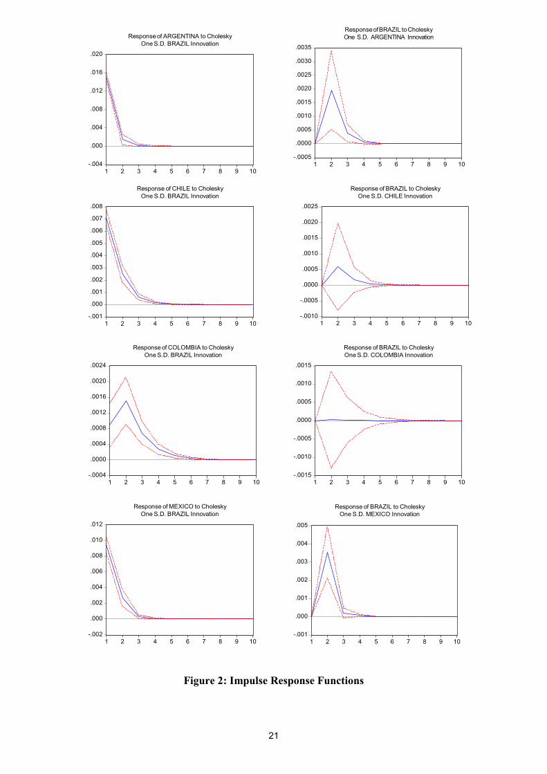
4.4. Impulse Response Functions
We present the impulse response functions for Latin American stock market indexes.
Parameters were estimated using the VAR described in section 2.3. Each impulse
response function (IRF) comes from shocking one of the variables, while holding other
variables constant. These IRF are shown with a 95% confidence interval, which were
obtained running Monte Carlo simulation (1000 repetitions). In the VAR’s the lags were
chosen using the Schwarz information criterion (more parsimonious model).
Using these IRF we can see that although there is bicausality between Argentina and the
Brazilian stock market the responses are quite different. The peak impact in Argentina is
felt with a one-day lag while in Brazil with a two-days lag. Furthermore, the magnitude
17
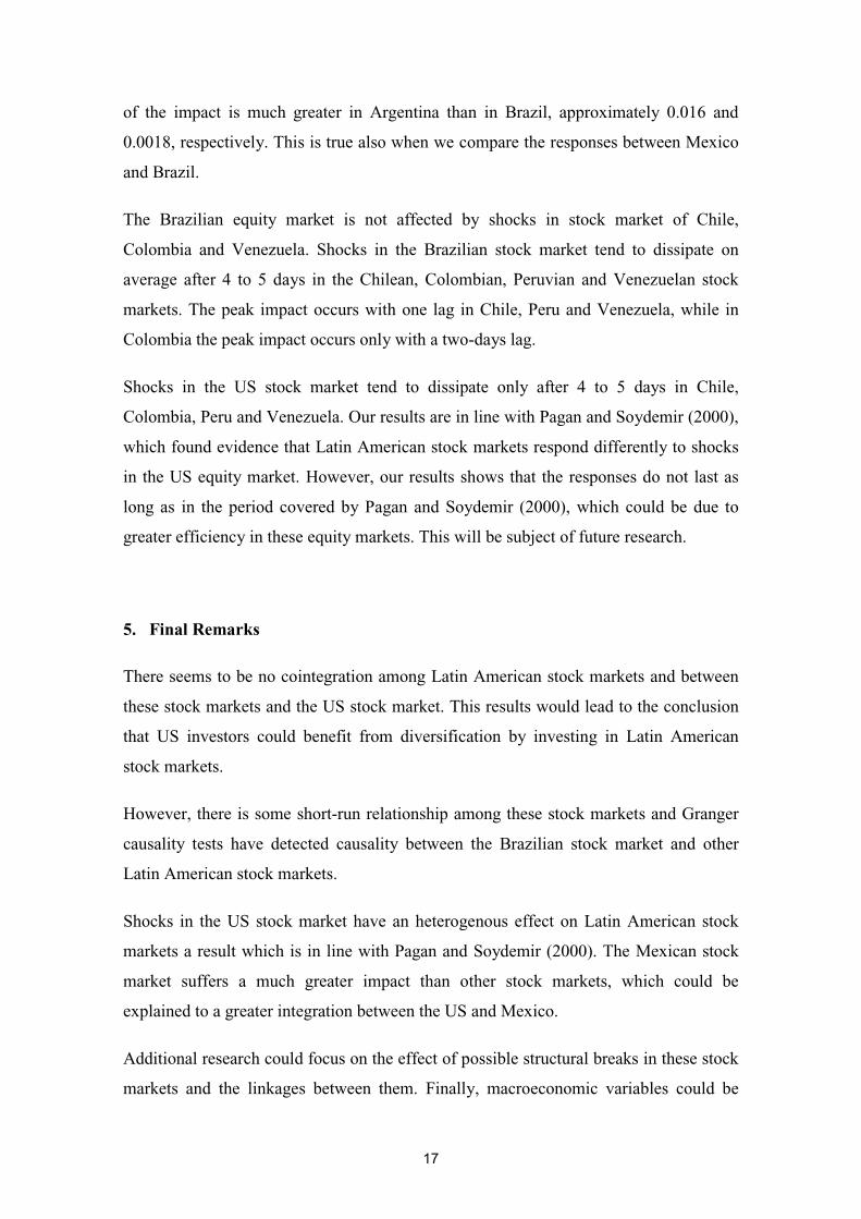
of the impact is much greater in Argentina than in Brazil, approximately 0.016 and
0.0018, respectively. This is true also when we compare the responses between Mexico
and Brazil.
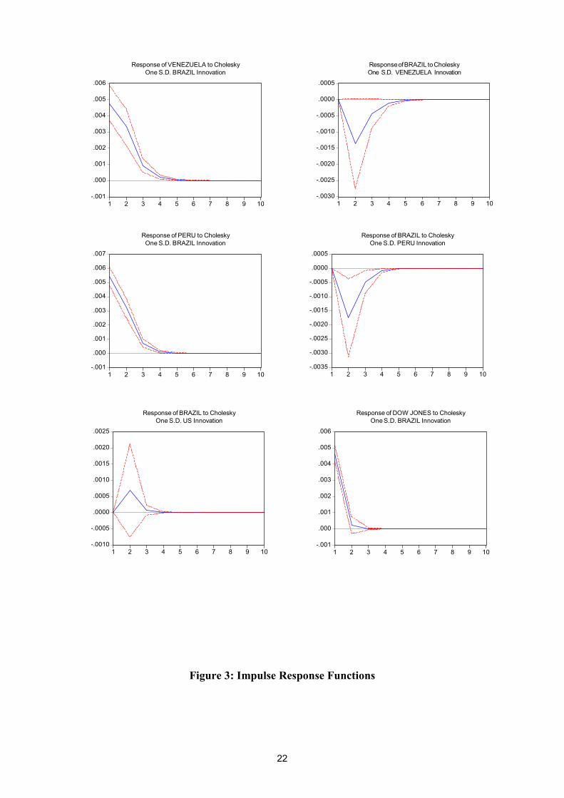
The Brazilian equity market is not affected by shocks in stock market of Chile,
Colombia and Venezuela. Shocks in the Brazilian stock market tend to dissipate on
average after 4 to 5 days in the Chilean, Colombian, Peruvian and Venezuelan stock
markets. The peak impact occurs with one lag in Chile, Peru and Venezuela, while in
Colombia the peak impact occurs only with a two-days lag.
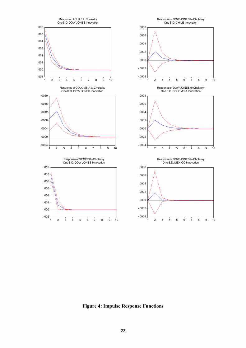
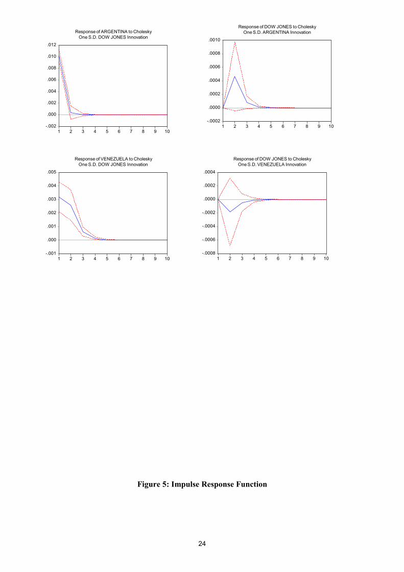
Shocks in the US stock market tend to dissipate only after 4 to 5 days in Chile,
Colombia, Peru and Venezuela. Our results are in line with Pagan and Soydemir (2000),
which found evidence that Latin American stock markets respond differently to shocks
in the US equity market. However, our results shows that the responses do not last as
long as in the period covered by Pagan and Soydemir (2000), which could be due to
greater efficiency in these equity markets. This will be subject of future research.
5. Final Remarks
There seems to be no cointegration among Latin American stock markets and between
these stock markets and the US stock market. This results would lead to the conclusion
that US investors could benefit from diversification by investing in Latin American
stock markets.
However, there is some short-run relationship among these stock markets and Granger
causality tests have detected causality between the Brazilian stock market and other
Latin American stock markets.
Shocks in the US stock market have an heterogenous effect on Latin American stock
markets a result which is in line with Pagan and Soydemir (2000). The Mexican stock
market suffers a much greater impact than other stock markets, which could be
explained to a greater integration between the US and Mexico.
Additional research could focus on the effect of possible structural breaks in these stock
markets and the linkages between them. Finally, macroeconomic variables could be

18
introduced in the analysis to link stock market relationships which were found in this
paper with variables such as exports, business cycles and monetary policy.
19
References
Aggarwal, R and Rivoli, P. (1989) “The relationship between the US and four Asian stock markets”. ASEAN Economic Bulletin 6(1), 110-117.
Arshanapali, B. and Doukas, J (1993) “International markets linkages: evidence from the pre- and post-October 1987 period”. Journal of Banking and Finance 17, 193-208.
Cheung, Y-W. and Lai, K.S. (1993) “Finite-sample sizes of Johansen’s likelihood ratio tests for cointegration”. Oxford Bulletin of Economics and Statistics 55,313-328.
Cheung, Y.L. and Mak, S.C. (1992) “The international transmission of stock markets fluctuation between the developed markets and the Asian-Pacific markets”. Applied Financial Economics 2, 43-47.
Dickey, D.A. and W.A. Fuller (1979) “Distribution of the Estimators for Autoregressive Time Series with a Unit Root”. Journal of the American Statistical Association, 74, 427–431.
Engle, Robert F. and C.W.J. Granger (1987) “Co-integration and Error Correction: Representation, Estimation, and Testing”. Econometrica 55, 251–276.
Gerrits, R. and Yuce, A. (1999) “Short- and Long-term Links among European and Us stock Markets”. Applied Financial Economics, 9, 1-9.
Granger, C. W. .J. (1969) “Investigating Causal Relations by Econometric Models and Cross-Spectral Methods”. Econometrica, 37, 424–438.
Hamilton, James D. (1994) “Time Series Analysis”. Princeton University Press.
Johansen, Soren (1991) “Estimation and Hypothesis Testing of Cointegration Vectors in Gaussian Vector Autoregressive Models”. Econometrica, 59, 1551–1580.
Johansen, S. and Juselius, K. (1990) “Maximum likelihood estimation and inference on cointegration with application to the demand of money”. Oxford Bulletin of Economics and Statistics 52, 169-210.
Kanas, A. (1998) “Linkages between the US and European Equity Markets: further evidence from cointegration tests”. Applied Financial Economics, 8, 607-614.
Osterwald-Lenum, M. (1992) “A noter with quantiles of the asymptotic distribution of the maximum likelihood cointegration rank test statistics. Oxford Bulletin of Economics and Statistics 54, 461-72.
Pagan, J.A. and Soydemir, G. (2000) “On the Linkages between equity markets in Latin America”. Applied Economics Letters 7, 207-210.
Phillips, P.C.B. and P. Perron (1988) “Testing for a Unit Root in Time Series Regression”. Biometrika, 75, 335–346.
SAS/ETS (1988) “User´s Guide”. Version 6, First Edition. SAS Institute Inc., Cary. NC, USA.
20
Figure 1: Stock Indexes
DOW JONES
0
50
100
150
200
250
300
350
Jan
-95
Ap
r-95
Jul-
95
Oct
-95
Jan
-96
Ap
r-96
Jul-
96
Oct
-96
Jan
-97
Ap
r-97
Jul-
97
Oct
-97
Jan
-98
Ap
r-98
Jul-
98
Oct
-98
Jan
-99
Ap
r-99
Jul-
99
Oct
-99
Jan
-00
Ap
r-00
Jul-
00
Oct
-00
Jan
-01
BRAZIL
0
50
100
150
200
250
300
Jan
-95
Ap
r-95
Jul-
95
Oct
-95
Jan
-96
Ap
r-96
Jul-
96
Oct
-96
Jan
-97
Ap
r-97
Jul-
97
Oct
-97
Jan
-98
Ap
r-98
Jul-
98
Oct
-98
Jan
-99
Ap
r-99
Jul-
99
Oct
-99
Jan
-00
Ap
r-00
Jul-
00
Oct
-00
Jan
-01
ARGENTINA
0
20
40
60
80
100
120
140
160
180
200
Jan
-95
Ap
r-95
Jul-
95
Oct
-95
Jan
-96
Ap
r-96
Jul-
96
Oct
-96
Jan
-97
Ap
r-97
Jul-
97
Oct
-97
Jan
-98
Ap
r-98
Jul-
98
Oct
-98
Jan
-99
Ap
r-99
Jul-
99
Oct
-99
Jan
-00
Ap
r-00
Jul-
00
Oct
-00
Jan
-01
MEXICO
0
50
100
150
200
250
Jan
-95
Ap
r-95
Jul-
95
Oct
-95
Jan
-96
Ap
r-96
Jul-
96
Oct
-96
Jan
-97
Ap
r-97
Jul-
97
Oct
-97
Jan
-98
Ap
r-98
Jul-
98
Oct
-98
Jan
-99
Ap
r-99
Jul-
99
Oct
-99
Jan
-00
Ap
r-00
Jul-
00
Oct
-00
Jan
-01
COLOMBIA
0
20
40
60
80
100
120
140
Jan
-95
Ap
r-95
Jul-
95
Oct
-95
Jan
-96
Ap
r-96
Jul-
96
Oct
-96
Jan
-97
Ap
r-97
Jul-
97
Oct
-97
Jan
-98
Ap
r-98
Jul-
98
Oct
-98
Jan
-99
Ap
r-99
Jul-
99
Oct
-99
Jan
-00
Ap
r-00
Jul-
00
Oct
-00
Jan
-01
CHILE
0
20
40
60
80
100
120
140
Jan
-95
Ap
r-95
Jul-
95
Oct
-95
Jan
-96
Ap
r-96
Jul-
96
Oct
-96
Jan
-97
Ap
r-97
Jul-
97
Oct
-97
Jan
-98
Ap
r-98
Jul-
98
Oct
-98
Jan
-99
Ap
r-99
Jul-
99
Oct
-99
Jan
-00
Ap
r-00
Jul-
00
Oct
-00
Jan
-01
VENEZUELA
0
50
100
150
200
250
300
350
Jan
-95
Ap
r-95
Jul-
95
Oct
-95
Jan
-96
Ap
r-96
Jul-
96
Oct
-96
Jan
-97
Ap
r-97
Jul-
97
Oct
-97
Jan
-98
Ap
r-98
Jul-
98
Oct
-98
Jan
-99
Ap
r-99
Jul-
99
Oct
-99
Jan
-00
Ap
r-00
Jul-
00
Oct
-00
Jan
-01
PERU
0
20
40
60
80
100
120
140
Jan
-95
Ap
r-95
Jul-
95
Oct
-95
Jan
-96
Ap
r-96
Jul-
96
Oct
-96
Jan
-97
Ap
r-97
Jul-
97
Oct
-97
Jan
-98
Ap
r-98
Jul-
98
Oct
-98
Jan
-99
Ap
r-99
Jul-
99
Oct
-99
Jan
-00
Ap
r-00
Jul-
00
Oct
-00
Jan
-01
21
Figure 2: Impulse Response Functions
-.004
.000
.004
.008
.012
.016
.020
1 2 3 4 5 6 7 8 9 10
Response of ARGENTINA to CholeskyOne S.D. BRAZIL Innovation
-.0005
.0000
.0005
.0010
.0015
.0020
.0025
.0030
.0035
1 2 3 4 5 6 7 8 9 10
Response of BRAZIL to CholeskyOne S.D. ARGENTINA Innovation
-.001
.000
.001
.002
.003
.004
.005
.006
.007
.008
1 2 3 4 5 6 7 8 9 10
Response of CHILE to CholeskyOne S.D. BRAZIL Innovation
-.0010
-.0005
.0000
.0005
.0010
.0015
.0020
.0025
1 2 3 4 5 6 7 8 9 10
Response of BRAZIL to CholeskyOne S.D. CHILE Innovation
-.0004
.0000
.0004
.0008
.0012
.0016
.0020
.0024
1 2 3 4 5 6 7 8 9 10
Response of COLOMBIA to CholeskyOne S.D. BRAZIL Innovation
-.0015
-.0010
-.0005
.0000
.0005
.0010
.0015
1 2 3 4 5 6 7 8 9 10
Response of BRAZIL to CholeskyOne S.D. COLOMBIA Innovation
-.002
.000
.002
.004
.006
.008
.010
.012
1 2 3 4 5 6 7 8 9 10
Response of MEXICO to CholeskyOne S.D. BRAZIL Innovation
-.001
.000
.001
.002
.003
.004
.005
1 2 3 4 5 6 7 8 9 10
Response of BRAZIL to CholeskyOne S.D. MEXICO Innovation
22
Figure 3: Impulse Response Functions
-.001
.000
.001
.002
.003
.004
.005
.006
1 2 3 4 5 6 7 8 9 10
Response of VENEZUELA to CholeskyOne S.D. BRAZIL Innovation
-.0030
-.0025
-.0020
-.0015
-.0010
-.0005
.0000
.0005
1 2 3 4 5 6 7 8 9 10
Response of BRAZIL to CholeskyOne S.D. VENEZUELA Innovation
-.001
.000
.001
.002
.003
.004
.005
.006
.007
1 2 3 4 5 6 7 8 9 10
Response of PERU to CholeskyOne S.D. BRAZIL Innovation
-.0035
-.0030
-.0025
-.0020
-.0015
-.0010
-.0005
.0000
.0005
1 2 3 4 5 6 7 8 9 10
Response of BRAZIL to CholeskyOne S.D. PERU Innovation
-.001
.000
.001
.002
.003
.004
.005
.006
1 2 3 4 5 6 7 8 9 10
Response of DOW JONES to CholeskyOne S.D. BRAZIL Innovation
-.0010
-.0005
.0000
.0005
.0010
.0015
.0020
.0025
1 2 3 4 5 6 7 8 9 10
Response of BRAZIL to CholeskyOne S.D. US Innovation
23
Figure 4: Impulse Response Functions
-.001
.000
.001
.002
.003
.004
.005
.006
1 2 3 4 5 6 7 8 9 10
Response of CHILE to CholeskyOne S.D. DOW JONES Innovation
-.0004
-.0002
.0000
.0002
.0004
.0006
.0008
1 2 3 4 5 6 7 8 9 10
Response of DOW JONES to CholeskyOne S.D. CHILE Innovation
-.0004
.0000
.0004
.0008
.0012
.0016
.0020
1 2 3 4 5 6 7 8 9 10
Response of COLOMBIA to CholeskyOne S.D. DOW JONES Innovation
-.0004
-.0002
.0000
.0002
.0004
.0006
.0008
1 2 3 4 5 6 7 8 9 10
Response of DOW JONES to CholeskyOne S.D. COLOMBIA Innovation
-.002
.000
.002
.004
.006
.008
.010
.012
1 2 3 4 5 6 7 8 9 10
Response of MEXICO to CholeskyOne S.D. DOW JONES Innovation
-.0004
-.0002
.0000
.0002
.0004
.0006
.0008
1 2 3 4 5 6 7 8 9 10
Response of DOW JONES to CholeskyOne S.D. MEXICO Innovation
24
Figure 5: Impulse Response Function
-.002
.000
.002
.004
.006
.008
.010
.012
1 2 3 4 5 6 7 8 9 10
Response of ARGENTINA to CholeskyOne S.D. DOW JONES Innovation
-.0002
.0000
.0002
.0004
.0006
.0008
.0010
1 2 3 4 5 6 7 8 9 10
Response of DOW JONES to CholeskyOne S.D. ARGENTINA Innovation
-.001
.000
.001
.002
.003
.004
.005
1 2 3 4 5 6 7 8 9 10
Response of VENEZUELA to CholeskyOne S.D. DOW JONES Innovation
-.0008
-.0006
-.0004
-.0002
.0000
.0002
.0004
1 2 3 4 5 6 7 8 9 10
Response of DOW JONES to CholeskyOne S.D. VENEZUELA Innovation
25
Banco Central do Brasil
Trabalhos para Discussão Os Trabalhos para Discussão podem ser acessados na internet, no formato PDF,
no endereço: http://www.bc.gov.br
Working Paper Series
Working Papers in PDF format can be downloaded from: http://www.bc.gov.br
1 Implementing Inflation Targeting in Brazil
Joel Bogdanski, Alexandre Antonio Tombini and Sérgio Ribeiro da Costa Werlang
July/2000
2 Política Monetária e Supervisão do Sistema Financeiro Nacional no Banco Central do Brasil Eduardo Lundberg Monetary Policy and Banking Supervision Functions on the Central Bank Eduardo Lundberg
Jul/2000
July/2000
3 Private Sector Participation: a Theoretical Justification of the Brazilian Position Sérgio Ribeiro da Costa Werlang
July/2000
4 An Information Theory Approach to the Aggregation of Log-Linear Models Pedro H. Albuquerque
July/2000
5 The Pass-Through from Depreciation to Inflation: a Panel Study Ilan Goldfajn and Sérgio Ribeiro da Costa Werlang
July/2000
6 Optimal Interest Rate Rules in Inflation Targeting Frameworks José Alvaro Rodrigues Neto, Fabio Araújo and Marta Baltar J. Moreira
July/2000
7 Leading Indicators of Inflation for Brazil Marcelle Chauvet
Set/2000
8 The Correlation Matrix of the Brazilian Central Bank’s Standard Model for Interest Rate Market Risk José Alvaro Rodrigues Neto
Set/2000
9 Estimating Exchange Market Pressure and Intervention Activity Emanuel-Werner Kohlscheen
Nov/2000
10 Análise do Financiamento Externo a uma Pequena Economia Aplicação da Teoria do Prêmio Monetário ao Caso Brasileiro: 1991–1998 Carlos Hamilton Vasconcelos Araújo e Renato Galvão Flôres Júnior
Mar/2001
11 A Note on the Efficient Estimation of Inflation in Brazil Michael F. Bryan and Stephen G. Cecchetti
Mar/2001
12 A Test of Competition in Brazilian Banking Márcio I. Nakane
Mar/2001
26
13 Modelos de Previsão de Insolvência Bancária no Brasil Marcio Magalhães Janot
Mar/2001
14 Evaluating Core Inflation Measures for Brazil Francisco Marcos Rodrigues Figueiredo
Mar/2001
15 Is It Worth Tracking Dollar/Real Implied Volatility? Sandro Canesso de Andrade and Benjamin Miranda Tabak
Mar/2001
16 Avaliação das Projeções do Modelo Estrutural do Banco Central do Brasil Para a Taxa de Variação do IPCA Sergio Afonso Lago Alves Evaluation of the Central Bank of Brazil Structural Model’s Inflation Forecasts in an Inflation Targeting Framework Sergio Afonso Lago Alves
Mar/2001
July/2001
17 Estimando o Produto Potencial Brasileiro: uma Abordagem de Função de Produção Tito Nícias Teixeira da Silva Filho Estimating Brazilian Potential Output: a Production Function Approach Tito Nícias Teixeira da Silva Filho
Abr/2001
Aug/2002
18 A Simple Model for Inflation Targeting in Brazil Paulo Springer de Freitas and Marcelo Kfoury Muinhos
Apr/2001
19 Uncovered Interest Parity with Fundamentals: a Brazilian Exchange Rate Forecast Model Marcelo Kfoury Muinhos, Paulo Springer de Freitas and Fabio Araújo
May/2001
20 Credit Channel without the LM Curve Victorio Y. T. Chu and Márcio I. Nakane
May/2001
21 Os Impactos Econômicos da CPMF: Teoria e Evidência Pedro H. Albuquerque
Jun/2001
22 Decentralized Portfolio Management Paulo Coutinho and Benjamin Miranda Tabak
June/2001
23 Os Efeitos da CPMF sobre a Intermediação Financeira Sérgio Mikio Koyama e Márcio I. Nakane
Jul/2001
24 Inflation Targeting in Brazil: Shocks, Backward-Looking Prices, and IMF Conditionality Joel Bogdanski, Paulo Springer de Freitas, Ilan Goldfajn and Alexandre Antonio Tombini
Aug/2001
25 Inflation Targeting in Brazil: Reviewing Two Years of Monetary Policy 1999/00 Pedro Fachada
Aug/2001
26 Inflation Targeting in an Open Financially Integrated Emerging Economy: the Case of Brazil Marcelo Kfoury Muinhos
Aug/2001
27
Complementaridade e Fungibilidade dos Fluxos de Capitais Internacionais Carlos Hamilton Vasconcelos Araújo e Renato Galvão Flôres Júnior
Set/2001
27
28
Regras Monetárias e Dinâmica Macroeconômica no Brasil: uma Abordagem de Expectativas Racionais Marco Antonio Bonomo e Ricardo D. Brito
Nov/2001
29 Using a Money Demand Model to Evaluate Monetary Policies in Brazil Pedro H. Albuquerque and Solange Gouvêa
Nov/2001
30 Testing the Expectations Hypothesis in the Brazilian Term Structure of Interest Rates Benjamin Miranda Tabak and Sandro Canesso de Andrade
Nov/2001
31 Algumas Considerações sobre a Sazonalidade no IPCA Francisco Marcos R. Figueiredo e Roberta Blass Staub
Nov/2001
32 Crises Cambiais e Ataques Especulativos no Brasil Mauro Costa Miranda
Nov/2001
33 Monetary Policy and Inflation in Brazil (1975-2000): a VAR Estimation André Minella
Nov/2001
34 Constrained Discretion and Collective Action Problems: Reflections on the Resolution of International Financial Crises Arminio Fraga and Daniel Luiz Gleizer
Nov/2001
35 Uma Definição Operacional de Estabilidade de Preços Tito Nícias Teixeira da Silva Filho
Dez/2001
36 Can Emerging Markets Float? Should They Inflation Target? Barry Eichengreen
Feb/2002
37 Monetary Policy in Brazil: Remarks on the Inflation Targeting Regime, Public Debt Management and Open Market Operations Luiz Fernando Figueiredo, Pedro Fachada and Sérgio Goldenstein
Mar/2002
38 Volatilidade Implícita e Antecipação de Eventos de Stress: um Teste para o Mercado Brasileiro Frederico Pechir Gomes
Mar/2002
39 Opções sobre Dólar Comercial e Expectativas a Respeito do Comportamento da Taxa de Câmbio Paulo Castor de Castro
Mar/2002
40 Speculative Attacks on Debts, Dollarization and Optimum Currency Areas Aloisio Araujo and Márcia Leon
Abr/2002
41 Mudanças de Regime no Câmbio Brasileiro Carlos Hamilton V. Araújo e Getúlio B. da Silveira Filho
Jun/2002
42 Modelo Estrutural com Setor Externo: Endogenização do Prêmio de Risco e do Câmbio Marcelo Kfoury Muinhos, Sérgio Afonso Lago Alves e Gil Riella
Jun/2002
43 The Effects of the Brazilian ADRs Program on Domestic Market Efficiency Benjamin Miranda Tabak and Eduardo José Araújo Lima
June/2002
44 Estrutura Competitiva, Produtividade Industrial e Liberação Comercial no Brasil Pedro Cavalcanti Ferreira e Osmani Teixeira de Carvalho Guillén
Jun/2002
28
45 Optimal Monetary Policy, Gains from Commitment, and Inflation Persistence André Minella
Aug/2002
46 The Determinants of Bank Interest Spread in Brazil Tarsila Segalla Afanasieff, Priscilla Maria Villa Lhacer and Márcio I. Nakane
Aug/2002
47 Indicadores Derivados de Agregados Monetários Fernando de Aquino Fonseca Neto e José Albuquerque Júnior
Sep/2002
48 Should Government Smooth Exchange Rate Risk? Ilan Goldfajn and Marcos Antonio Silveira
Sep/2002
49 Desenvolvimento do Sistema Financeiro e Crescimento Econômico no Brasil: Evidências de Causalidade Orlando Carneiro de Matos
Set/2002
50 Macroeconomic Coordination and Inflation Targeting in a Two-Country Model Eui Jung Chang, Marcelo Kfoury Muinhos and Joanílio Rodolpho Teixeira
Sep/2002
51 Credit Channel with Sovereign Credit Risk: an Empirical Test Victorio Yi Tson Chu
Sep/2002
52 Generalized Hyperbolic Distributions and Brazilian Data José Fajardo and Aquiles Farias
Sep/2002
53 Inflation Targeting in Brazil: Lessons and Challenges André Minella, Paulo Springer de Freitas, Ilan Goldfajn and Marcelo Kfoury Muinhos
Nov/2002
54 Stock Returns and Volatility Benjamin Miranda Tabak and Solange Maria Guerra
Nov/2002
55 Componentes de Curto e Longo Prazo das Taxas de Juros no Brasil Carlos Hamilton Vasconcelos Araújo e Osmani Teixeira de Carvalho de Guillén
Nov/2002