Embed Size (px)
Citation preview
ISSN 1561081-0
9 7 7 1 5 6 1 0 8 1 0 0 5
WORKING PAPER SER IESNO 719 / JANUARY 2007
US IMBALANCES
THE ROLE OF TECHNOLOGY AND POLICY
by Rudolfs Bems, Luca Dedola and Frank Smets
In 2007 all ECB publications
feature a motif taken from the €20 banknote.
WORK ING PAPER SER IE SNO 719 / JANUARY 2007
This paper can be downloaded without charge from http://www.ecb.int or from the Social Science Research Network
electronic library at http://ssrn.com/abstract_id=957615.
US IMBALANCES
THE ROLE OF TECHNOLOGY AND
POLICY 1
by Rudolfs Bems 2, Luca Dedola 2
and Frank Smets 2
1 We thank Helen Popper and Mark Taylor, our discussants at the conference on “The euro and the dollar in globalised economy” in Santa Cruz and the conference on “Financial globalisation and integration” in Frankfurt for very useful comments. The views
expressed are solely our own and do not reflect those of the European Central Bank. 2 Correspondence: European Central Bank, Kaiserstrasse 29, 60311 Frankfurt am Main, Germany;
e-mail: [email protected]; [email protected]; [email protected]
© European Central Bank, 2007
AddressKaiserstrasse 2960311 Frankfurt am Main, Germany
Postal addressPostfach 16 03 1960066 Frankfurt am Main, Germany
Telephone +49 69 1344 0
Internethttp://www.ecb.int
Fax +49 69 1344 6000
Telex411 144 ecb d
All rights reserved.
Any reproduction, publication and reprint in the form of a different publication, whether printed or produced electronically, in whole or in part, is permitted only with the explicit written authorisation of the ECB or the author(s).
The views expressed in this paper do not necessarily reflect those of the European Central Bank.
The statement of purpose for the ECB Working Paper Series is available from the ECB website, http://www.ecb.int.
ISSN 1561-0810 (print)ISSN 1725-2806 (online)
3ECB
Working Paper Series No 719January 2007
CONTENTS
Abstract 4Non-technical summary 51 Introduction 72 The impact of technology and policy shocks on the US trade balance: VAR evidence 9 2.1 Technology 10 2.2 Fiscal policy 14 2.3 Monetary policy 183 The contribution of technology and policy to US current account developments 21Conclusions 24Appendix: The identification scheme of the VAR estimated in Section 3 25References 26Tables and figures 30European Central Bank Working Paper Series 39
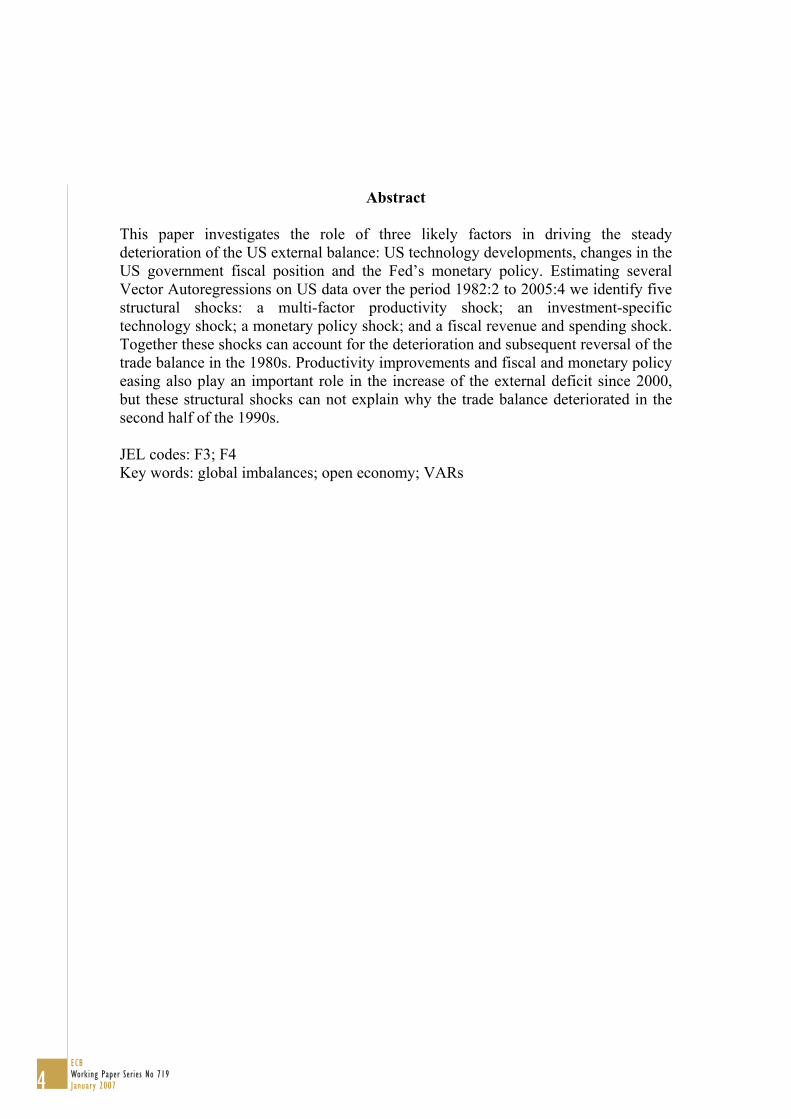
Abstract
This paper investigates the role of three likely factors in driving the steady deterioration of the US external balance: US technology developments, changes in the US government fiscal position and the Fed’s monetary policy. Estimating several Vector Autoregressions on US data over the period 1982:2 to 2005:4 we identify five structural shocks: a multi-factor productivity shock; an investment-specific technology shock; a monetary policy shock; and a fiscal revenue and spending shock. Together these shocks can account for the deterioration and subsequent reversal of the trade balance in the 1980s. Productivity improvements and fiscal and monetary policy easing also play an important role in the increase of the external deficit since 2000, but these structural shocks can not explain why the trade balance deteriorated in the second half of the 1990s.
Key words: global imbalances; open economy; VARs
JEL codes: F3; F4
4ECB Working Paper Series No 719January 2007
Non-technical summary Since the early 1990s the US current account and net trade deficit have steadily
deteriorated from close to balance to a deficit of more than 5 percent in 2004 and
2005. As a counterpart, various regions have developed large surpluses vis-à-vis the
United States. The emergence of those global current account imbalances has
generated a large literature investigating the sources of the imbalances, their
sustainability and the likely adjustment mechanism including the role of the exchange
rate in this adjustment and the implications of the adjustment process for global
growth and financial markets. Clearly, both the sustainability and the features of the
adjustment mechanism depend very much on the sources behind the emergence of the
imbalances. A number of authors have focused on developments in the US economy,
in particular the productivity boom starting in the second half of the 1990s, but also
developments in fiscal and monetary policy in particular since the start of the new
millennium. Others have emphasized excess savings in Asian countries pointing out
that following the Asian crisis in 1997 savings rates in many Asian countries
remained relatively high in spite of falling investment rates. Still others have
highlighted the efforts of some Asian monetary authorities to resist an appreciation of
their respective currencies and to accumulate large quantities of foreign reserves.
Finally, more recently the recycling of the increased oil revenues by oil-producing
countries has been pointed out as a major factor.
In this paper, we focus on the role of domestic US factors. The main reason for doing
so is that the secular deterioration of the net trade balance has occurred relative to
most of the major regions in the world. This suggests that some of the main sources
are likely to lie in developments in the United States itself. The paper investigates the
role of three likely factors: US productivity developments and the new-economy
boom, changes in the fiscal position of the US government and the Fed’s monetary
policy. For that purpose we estimate Vector Autoregressions (VARs) on US data over
the period from 1982 to 2005 and identify various structural shocks: multi-factor
productivity shocks; investment-specific or embodied technology shocks, monetary
5ECB
Working Paper Series No 719January 2007
the trade balance can be explained by those shocks. We find that each of the structural
shocks have an economically and often statistically significant impact on the trade
balance more or less in line with a priori reasoning: Positive technology shocks and
expansionary fiscal and monetary policy developments lead to a deterioration of the
trade balance. Together the shocks explain the deterioration of the trade balance in the
early 1980s and its subsequent return to balance in the second half of the 1980s. They
also explain the deterioration of the trade balance in the new millennium. Both
positive technology developments and fiscal and monetary policy easing following
the collapse of the dot-com bubble play an important role in the rapid deterioration
since 2000. Somewhat surprisingly, the estimated technology shocks can not account
for the increase in the trade deficit in the second half of the 1990s.
6ECB Working Paper Series No 719January 2007
policy shocks and fiscal revenue and expenditure shocks. We analyze the effects of
those shocks on the current account and investigate how much of the developments in
1. Introduction Since the early 1990s the US current account and net trade deficit have steadily
deteriorated from close to balance to a deficit of more than 5 percent in 2004 and
2005 (see Figure 1). As a counterpart, a number of countries/regions have developed
large surpluses vis-à-vis the United States (Figure 2). The emergence of those global
current account imbalances has generated a large literature investigating the sources
of the imbalances, their sustainability and the likely adjustment mechanism including
the role of the exchange rate in this adjustment and the implications of the adjustment
process for global growth and financial markets.1 Clearly, both the sustainability and
the features of the adjustment mechanism depend very much on the sources behind
the emergence of the imbalances. A number of authors have focused on developments
in the US economy, in particular the productivity boom starting in the second half of
the 1990s, but also developments in fiscal and monetary policy in particular since the
start of the new millennium.2 Others have emphasized excess savings in Asian
countries pointing out that following the Asian crisis in 1997 savings rates in many
Asian countries remained relatively high in spite of falling investment rates.3 Still
others have highlighted the efforts of some Asian monetary authorities to resist an
appreciation of their respective currencies and to accumulate large quantities of
foreign reserves.4 Finally, more recently the recycling of the increased oil revenues by
oil-producing countries has been pointed out as a major factor (e.g. WEO, 2006).5
{Insert Figure 1}
In this paper, we focus on the role of domestic US factors. The main reason for doing
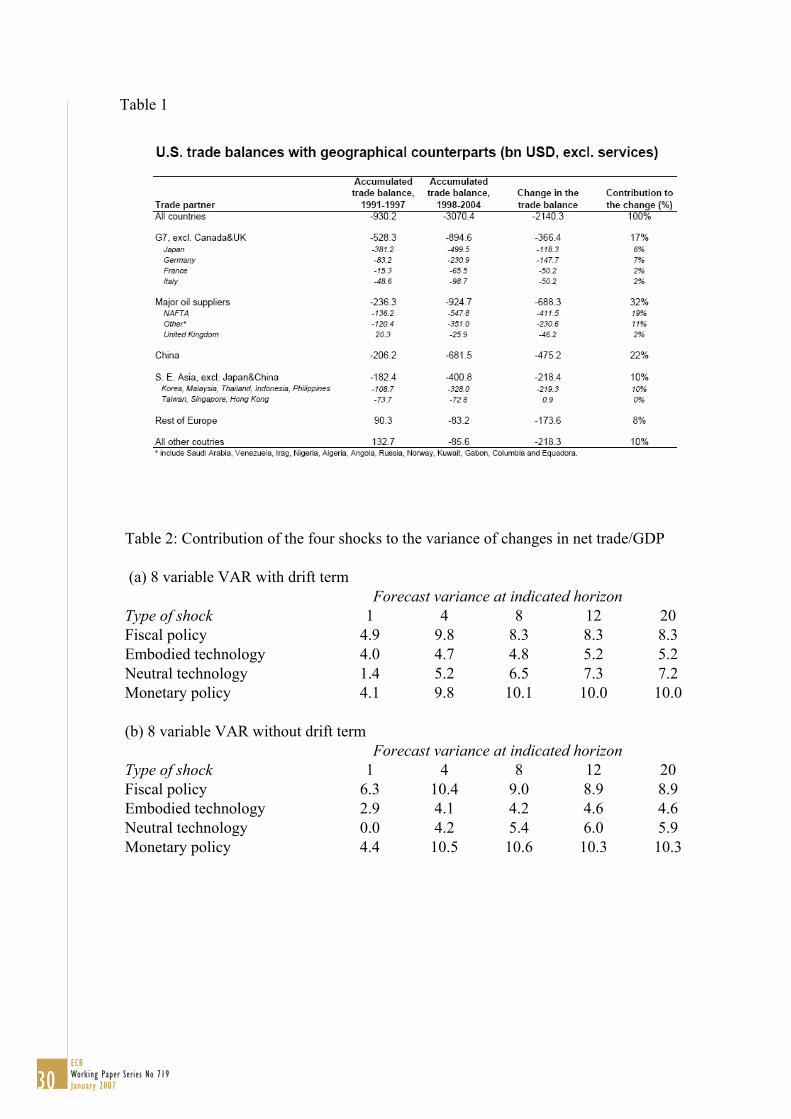
so is that, as illustrated in Table 1, the secular deterioration of the net trade balance
has occurred relative to most of the major regions in the world. This suggests that
some of the main sources are likely to lie in developments in the United States itself. 1 For a recent more academic survey see Corsetti (2005). Policy surveys are Gros, Mayer and Ubide (2006), WEO (2005), BIS (2004). 2 Examples are Engel and Rogers (2006), Backus et al (2006), Roubini and Setzer (2005). 3 See, for example, Bernanke (2005), Caballero, Gourinchas and Fahri (2005), WEO (2005). 4 See, for example, Dooley, Folkerts-Landau and Garber (2005). 5 In addition, there is a quite lively literature on measurement issues ranging from papers that argue the US is not a deficit country (Hausmann and Sturzenegger 2005) to papers that argue that the problem may be even more serious than suggested by conventional measurement (Gros et al, 2006).
7ECB
Working Paper Series No 719January 2007
{Insert Table 1}
The paper investigates the role of three likely factors: US productivity developments
and the new-economy boom, changes in the fiscal position of the US government and
the Fed’s monetary policy. For that purpose we estimate Vector Autoregressions
(VARs) on US data and identify various structural shocks: a multi-factor productivity
shock; an investment-specific or embodied technology shock, a monetary policy
shock and a fiscal revenue and expenditure shock. In Section 2, we analyze the effects
of those shocks separately following and extending an extensive academic literature
that uses VARs to investigate the role of those shocks in US business cycles. In
Section 2.1, we identify the technology shocks using long-run zero restrictions on
labour productivity and the relative price of investment equipment respectively
following Gali (1999) and Fischer (2006). Section 2.2 focuses on the role of fiscal
policy and following Perotti (2005) uses contemporaneous zero restrictions to identify
both government spending and revenue shocks. Finally, Section 2.3 analyses the role
of monetary policy shocks as in Christiano, Eichenbaum and Evans (1999) and Kim
(2001).
As argued in Altig et al (2005), a number of those shocks can account for a large
fraction of business cycle fluctuations in the United States. It is therefore interesting
to see how much of the developments in the trade balance can be explained by those
shocks. An important caveat to this US-focused approach is that only asymmetric
shocks are likely to affect current account and trade balances (Glick and Rogoff,
1995). Ignoring the international comovement and transmission of the US shocks as
well as the incidence of foreign shocks may bias our results. However, the direction of
this bias is not clear. To the extent that the identified shocks are common across
countries, the estimated effects on the trade balance are likely to be underestimated. In
contrast, if domestic and foreign shocks are negatively correlated, the estimated
effects may be overestimated.6
6 In the case of productivity shocks, we have investigated the effect of identifying relative productivity shocks on the basis of relative labour productivity movements in the US versus the G7 countries. In this case, our estimates were not significantly affected.
8ECB Working Paper Series No 719January 2007
Notwithstanding these caveats, we find that each of the structural shocks have an
economically and often statistically significant impact on the trade balance more or
less in line with a priori reasoning: Positive technology shocks and expansionary
fiscal and monetary policy developments lead to a deterioration of the trade balance.
Together the shocks explain the deterioration of the trade balance in the early 1980s
and its subsequent return to balance in the second half of the 1980s. They also explain
the deterioration of the trade balance in the new millennium. Both positive technology
developments and fiscal and monetary policy easing following the collapse of the dot-
com bubble play an important role in the rapid deterioration since 2000. Somewhat
surprisingly, the estimated technology shocks can not account for the increase in the
trade deficit in the second half of the 1990s.
2. The impact of technology and policy shocks on the US trade balance: VAR evidence
In this section we discuss each of the three possible factors (technology, fiscal policy
and monetary policy) in turn. In each case, we examine the related VAR literature that
has tried to identify those shocks and analyze their effects on the trade balance. In
each of these sections, the empirical strategy is to first replicate a key VAR study in
the literature and to then extend the analysis by extending the sample to 2005:4 and
including the net trade/GDP ratio. For space reasons, in what follows, we only report
the findings from the final VAR.7
In order to estimate the effects of the various shocks, we use a common data sample
starting in the early 1980s (1982:2-2005:4 to be precise). There are various reasons
for restricting the analysis to the last two decades or so. First, given our interest in
understanding the US trade balance, it is important to focus on a period when the
international markets in goods, services and financial assets were more or less
liberalized. The 1980s was a period of general liberalization of international capital
movements in many regions of the world making the external financing of domestic
saving and investment imbalances easier. Second, Clarida, Gali and Gertler (2000)
have argued that there has been a change in the conduct of monetary policy associated
7 All quarterly VARs estimated in this paper contain four lags of the endogenous variables.
9ECB
Working Paper Series No 719January 2007
with the appointment of Paul Volker to the Federal Reserve. Gali, Lopez-Salido and
Valles (2003) present evidence that the change in policy regime has also led to a
change in the effects of neutral technology shocks on the US economy, while Boivin
and Giannoni (2005) argue that it has also impacted the effects of monetary policy.
Also Perotti (2005) and Fisher (2006) document pre-and-post-1982 sample
differences in the effects of fiscal policy and technology shocks respectively. Third, a
large literature starting with McConnell and Perez-Quiros (2000) has documented a
substantial decline in the volatility of many macro-economic variables after 1984. The
sources of this “great moderation” are still unclear.8 Alternative hypothesis are
changes in inventories, better stabilization policies and increased financial deepening
and integration leading to a relaxation of credit constraints. Fourth, Fisher (2006)
finds a structural break in the mean rate of decline in the baseline equipment deflator
around 1982 (0.84% versus 1.49% after 1982). He relates this to the time when the
personal computer began to be widely used in business. For all these reasons, we will
focus on the period 1982:2 – 2005:4 in the rest of the analysis.
2.1. Technology
The new economy boom of the 1990s and the increase in expected productivity
growth in the United States is one of the most-often cited factors that are used to
explain the deterioration of the current account since the 1990s. For example, Hunt
and Rebucci (2005) argue that a persistent increase in productivity in the
manufacturing/traded-goods sector associated with some learning can explain about
one third of the deterioration of the US trade balance over the period 1996-2000. In
this story foreign borrowing allows US households to consume part of their future
wealth and firms to invest in order to make use of new profitable technologies. It is
indeed a well-documented fact that over the past 15 years total factor productivity
growth in the US has increased relative to the rest of the G7 countries and the world
more generally. For example, recent estimates from the OECD show that US multi
factor productivity grew by almost 2 percent per year over the 1998-2004 period and
1 percentage point higher than during 1991-1997. In contrast, the other G7 countries
in general saw their productivity growth rates fall. At the same time, investment rates
8 See, for example, Stock and Watson (2005) for a recent investigation.
10ECB Working Paper Series No 719January 2007
boomed in the second half of the 1990s, suggesting that some of the new technologies
may have been embedded in new capital goods.
In this section, we therefore aim at identifying two kinds of technology shocks
(neutral - or multi-factor – and embodied technology shocks). There has been a lively
debate about the role of productivity shocks in accounting for business cycle
fluctuations in the United States. A number of authors (most prominently Galí (1999),
Francis and Ramey (2005) and Galí and Rabanal (2004)) have argued that total factor
productivity shocks can not account for a large fraction of US business cycles because
they lead to a negative correlation between output and hours worked in the face of
nominal rigidities, habit formation and adjustment costs in investment (See also Smets
and Wouters, forthcoming). Others such as Altig et al (2005) and Dedola and Neri
(2005) have argued that the empirical evidence on the effect of productivity on hours
worked could be consistent with a positive impact. Fisher (2006) argues that
investment-specific productivity shocks or embodied technology shocks can account
for a much larger fraction of business cycle fluctuations than neutral technology
shocks. Together they account for about 40 to 60 % of business cycle fluctuations, of
which embodied technology shocks account for the most part. Altig et al (2005),
using a different methodology, also argue that both productivity shocks can account
for a large fraction of GDP fluctuations.
In this Section we estimate Fisher’s (2006) VAR over the period 1982:2 – 2005:4 and
add the net trade/GDP ratio in order to estimate the effects of total factor productivity
and embodied technology shocks on net trade. As in Fisher (2006), the six-variable
VAR reported in this section includes the log change in the relative price of
equipment,9 the log change in labour productivity in the non-farm business, the
associated log per-capita hours worked, the log change in the GDP deflator and the
federal funds rate.10 In addition, we add the change in the net trade/GDP ratio11. The
two technology shocks are identified using long-run restrictions. In particular, the
embodied technology shock is the only shock that has a long-run impact on the 9 We thank Riccardo Di Cecio and Reinout de Boeck for providing us with this series until 2004:4. We extended it further using the NIPA deflators. 10 Fischer (2006) uses the same five-variable VAR for the sub-sample analysis, although in his specification a consumption deflator built by him replaces the GDP deflator in our analysis. 11 Using a battery of conventional unit root tests, we could not reject nonstationarity of this variable over the sample period.
11ECB
Working Paper Series No 719January 2007
relative price of equipment. Moreover, the embodied and neutral (or multi-factor)
productivity shocks are the only shocks that have a long-run impact on labour
productivity. Finally, using a stylized growth model Fischer (2006) shows that the
long-run impact of the embodied technology shock on labour productivity is related to
the share of capital in production and uses this restriction as an over-identifying
restriction.12
Precisely, denote the N variables in a VAR by Yt:
( )( )
.loglog
,...
,',1
21
1
⎥⎥⎥
⎦
⎤
⎢⎢⎢
⎣
⎡∆∆
=
+++≡
Σ=+=−
−
t
t
t
t
ttttt
Xzp
Y
LBLBBLB
uEuuYLBY
Here pt denotes the relative price of equipment, zt is labour productivity in the non-
farm business sector, and Xt is an additional vector of variables included in the VAR.
In all of our applications we assume that the number of lags q = 4. Suppose that the
fundamental economic shocks are related to the one-step ahead forecast error ut via
the relationship:
Σ=== ',', CCIeEeCeu tttt ,
where the first two elements in et are the embodied and neutral technology shocks,
respectively. To be able to compute the dynamic effects of the two shocks on the
elements of Yt we need the matrices Bi and the first two columns of C. Remember that
the two long-run restrictions imply that the long-run responses of the system R obey:
( )[ ]
⎥⎥⎥⎥⎥
⎦
⎤
⎢⎢⎢⎢⎢
⎣
⎡
=−≡
−−−−
−
−−
)2()2(,.
1)2(2,
1)2(1,
)2(121
)2(111 0
00
1
NxNX
xNX
xNX
Nxzz
Nxp
RRR
rr
r
CBIR .
The 0’s reflect the assumption that only the embodied technology shock has a non-
zero long-run impact on the relative price of equipment rp1 and only the embodied and
neutral productivity shocks have non-zero long-run impacts rz1 and rz2 on labour
productivity. Although we cannot directly estimate R, we can easily estimate RR’:
( )[ ] ( )[ ] 11 '1'1' −− −−≡ BICCBIRR ,
12 We find that in the extended sample, this restriction is rejected in the 6-variable VAR. Nevertheless, we still report the results obtained imposing it since they are very similar to those in the benchmark specification of Section 3, where the restriction is not imposed.
12ECB Working Paper Series No 719January 2007
since the Bi’s and the variance-covariance matrix Σ = CC’ can be obtained by
applying ordinary least squares to the VAR reduced form. Therefore, the first two
columns of C are obtained from the first two columns of the Choleski decomposition
of RR’. If Fisher’s over-identifying restriction on the long-run impact of the embodied
technology shock on labour productivity is also imposed, implying a proportionality
between rp1 and rz1, the two columns of C will not be simply equal their counterparts
in the Choleski decomposition, but the fully nonlinear system for RR’ above will need
to be solved.
{Insert Figure 2}
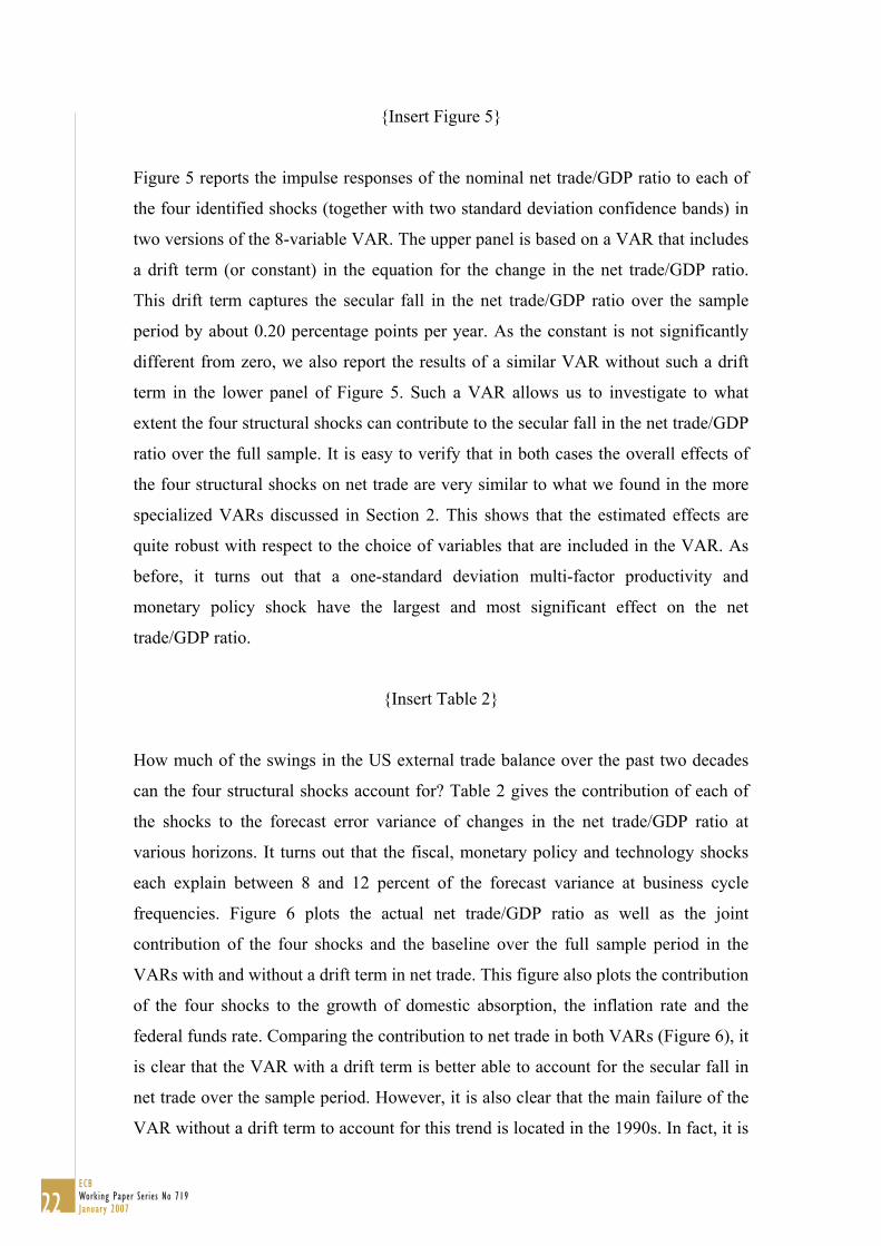
Figure 2 reports the impulse responses of each of the six variables to both shocks.13 A
number of similarities and differences between both shocks are worth noting. Both
increase labour productivity in the long run and lead to a fall in inflation although the
timing and the dynamics of the effects is quite different. However, the embodied
shock leads to a tightening of monetary policy, while the neutral shock leads to an
easing. Moreover, in agreement with the theory, hours worked increase in response to
the embodied shock, while they fall in response to the neutral shock. Most
interestingly, both shocks lead to a deterioration of the trade balance. However, the
impact of the neutral shock is a magnitude larger and more significant than that of the
embodied shock.14 A one percent increase in multi-factor productivity leads to an
estimated deterioration of the net trade/GDP ratio by 0.5 percentage points, whereas a
similar embodied technology shock has less than half this effect. At first sight, the
smaller impact of the embodied technology shock on net trade may seem somewhat
counterintuitive as it has a larger impact on absorption and therefore on imports.
However, note that partly due to the differential interest rate response the terms-of-
trade deterioration in the case of the neutral shock is likely to be much larger than in
the case of the embodied technology shock. This price effect will tend to dominate the
quantity effects on the nominal net trade to GDP ratio. This is indeed exactly what De
Walque, Smets and Wouters (2005) find in their estimated US-euro area DSGE
13 For clarity, in Figures 2 and 3 we have deleted the confidence bands in order to compare the impulse response of two shocks. The significance of the response of the net trade/GDP ratio is similar to that reported in Figures 5 and 6. 14 As also shown in Figure 5, the impact of the embodied technology shock on the nominal net trade/GDP ratio is not significant at the 5% confidence level.
13ECB
Working Paper Series No 719January 2007
model. While the investment-specific technology shock has a larger negative effect on
the real trade balance, the terms-of-trade response is much more favourable and tends
to dominate in the case of such shocks. De Walque et al (2005) also show that this
qualitative result is independent of whether a high or low elasticity of substitution is
assumed. These findings are also partially confirmed in our VAR analysis.
Substituting the real net trade/GDP ratio for the nominal one, we find that the impact
of the embodied technology shock on the real net trade/GDP ratio is indeed much
larger, reflecting the fact that the terms of trade improves following such a shock (not
shown).
The ability of the technology shocks to explain the developments in the US external
trade balance will be investigated in Section 3. Here it is, however, useful to compare
the size of the effects with some of the estimates in the literature. Bussiere et al (2005)
extend the study by Glick and Rogoff (1995) and find that a one percent asymmetric
productivity increase (as measured by total factor productivity) leads to a current
account deterioration of about 0.15 percentage points. Corsetti et al. (2006) look at the
effects of productivity shocks in manufacturing identified with long-run restrictions,
finding similar multipliers. Our estimates of the effect of a multi-factor productivity
shock are clearly larger, although those of the investment specific shock are
somewhat lower. This underlines the need for distinguishing between the various
technology shocks when examining their impact on external balances. The role of
productivity developments in accounting for the deterioration of the current account
in the late 1990s is also discussed in Hunt and Rebucci (2005) using a calibrated two-
country DSGE model. They conclude that the productivity shock needs to be
augmented with a negative risk premium shock on US assets in order to be able to
account for the full deterioration of the US trade deficit in the second half of the
1990s.
2.2. Fiscal policy
The twin deficit hypothesis that an increasing government deficit will result in a
deterioration of the current account balance is hotly debated. Historically, movements
in the general government surplus and the current account balance have hardly been
identical twins. While the U.S. trade balance deteriorated throughout the 1990-2005
14ECB Working Paper Series No 719January 2007
period, the general government budget position improved during the 90s and then fell
sharply after 2000. At the same time, the sharp fall in government revenues and rise in
government spending in 2001-2003 may have contributed to the accelerating fall of
the current account balance in that period. Similarly, the deterioration and subsequent
improvement of the current account in the 1980s may have been associated with the
rise and subsequent fall in the US government deficit in that period. Several recent
papers in the literature have re-examined the scope for twin deficits in the US data,
but no clear conclusions have been reached. For example, Kim and Roubini (2004)
find that government deficit and spending shocks have a positive effect on the trade
balance, in contrast to the theoretical literature on the twin deficit hypothesis which
would generally suggest a negative impact. Corsetti and Muller (2006) show that the
response of the current account to government spending shocks may depend on the
persistence of the shock as well as the degree of openness. In more open economies
and with more persistent shocks, investment will be crowded out less, as the
associated terms of trade improvement increases the rate of return on investment. As a
result, the twin deficit hypothesis may be valid for small open economies, but less so
for relatively closed economies such as the United States. Using a VAR analysis,
Corsetti and Muller (2006) find some evidence in favor of their analysis. Bussiere et
al (2005) perform a cross-country analysis of current account imbalances and
government deficits. They find that a 1 percentage point reduction in the government
deficit leads to less than a 0.1 percentage point deterioration of the current account.
This is at the lower end of the multipliers in a number of studies surveyed by Bussiere
et al (2005). For example, Erceg et al (2005), who use a calibrated modern DSGE
model, find a multiplier of 0.2.
Most of the literature focuses on government deficit or spending shocks. Theoretically
however, the effects of a deterioration in the government deficit on the current
account may be different depending on the source of the deterioration, in particular
whether it is due to increased government spending or reduced taxes.15 The
deterioration of the US government balance in 2001-2003 was mostly due to a fall in
government revenues following a series of tax reductions. It is therefore of interest to
look at both government spending and tax shocks.
15 For a recent survey of some of the theoretical literature see Kim and Roubini (2004).
15ECB
Working Paper Series No 719January 2007
In order to assess the effects of fiscal policy, one needs to take into account the other
shocks to the economy as well as the typical automatic stabilizers of fiscal policy. 16
In this section, we follow the work of Blanchard and Perotti (2002) and Perotti (2005)
to estimate the effects of fiscal revenue and spending shocks on the trade balance.17 18
The results that we report are based on Perotti (2005), since this study includes more
recent years and reports results for samples starting in the early 1980s. However,
similar findings were obtained by extending Blanchard and Perotti (2002). Apart from
a different sample period, the only difference with the VAR specification in Perotti
(2005) is the addition of net trade. Thus, our VAR specification includes 6 variables:
(i) the log of real per capita government spending on goods and services, including
government purchases and government investment, (ii) the log of real per capita net
primary revenues, defined as government revenues less government transfers,19 (iii)
the log of real per capita GDP, (iv) the log of GDP deflator, (v) ten year nominal
interest rate, (vi) ratio of nominal net exports over nominal GDP. For fiscal variables
and GDP, real values are obtained by deflating nominal values with the GDP deflator.
Equations in the VAR also include four lags and a constant term. To make results
directly comparable with the large-scale VAR results from the next section, all the
variables, except the 10 year nominal interest rate, are expressed in log first
differences.
Government spending and revenue shocks are identified using contemporaneous zero
restrictions. In the VAR government spending (G) and net taxes (T) are ordered first
and second, followed by real GDP, GDP deflator and the 10 year nominal interest
rate. Net trade is added to the VAR by ordering it last; namely Yt is defined as:
16 For an alternative story about the role of government debt policy in driving current account
17 A related study is Mountford and Uhlig (2005), who use sign restrictions rather than contemporaneous restrictions to identify fiscal policy shocks. 18 Blanchard and Perotti (2002) also report separate responses of exports and imports to the fiscal shocks, although it is not the main focus of the paper. 19 For exact definition of both fiscal series see Blanchard and Perotti (2002) or Mountford and Uhlig (2005). Spending and tax series from Perotti (2005) would be preferred here, but are not publicly available. These series should not be very different from the ones used in Blanchard and Perotti (2002) and Mountford and Uhlig (2005).
16ECB Working Paper Series No 719January 2007
imbalances in the early years of the millennium, see Kraay and Ventura (2005).
⎥⎥⎥
⎦
⎤
⎢⎢⎢
⎣
⎡∆∆
=t
t
t
t
XTG
Y loglog
,
where Xt includes the growth rates of real GDP and GDP deflator, the 10 year
nominal interest rate net trade over GDP . Remembering that the fundamental
economic shocks are related to the one-step ahead forecast error ut via the
relationship:
Σ=== ',', CCIeEeCeu tttt ,
the two fiscal shocks of interest, ordered first and second in et, are identified directly
restricting the (inverse of) matrix C, depicting how reduced form residuals map into
structural shocks. In order to be able to recover the first two columns of C, we need
N-1 + N-2 = 9 restrictions. We obtain them by positing reaction functions for the two
fiscal variables, following Perotti (2005). First, we assume that expenditure does not
contemporaneously react to revenues, and then is ordered first in the VAR.20 Second,
the contemporaneous responses of government spending and revenues to GDP and
prices are set on a priori basis. For our sample of interest (1982:2-2005:4) we apply
the elasticities that Perotti (2005) reports for the 1980Q1-2001Q4 period (see Table 4
in Perotti (2005), n[gy]=0; n[ty]=1.97; n[gp]=-0.5; n[tp]=1.4; n[gi]=0; n[ti]=0).
Finally, the last two restrictions needed are obtained by assuming that similar
elasticities concerning the trade balance are zero.
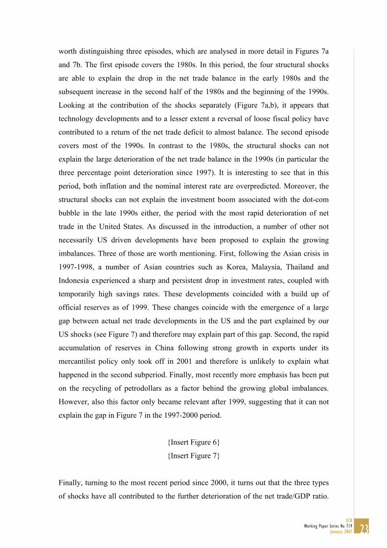
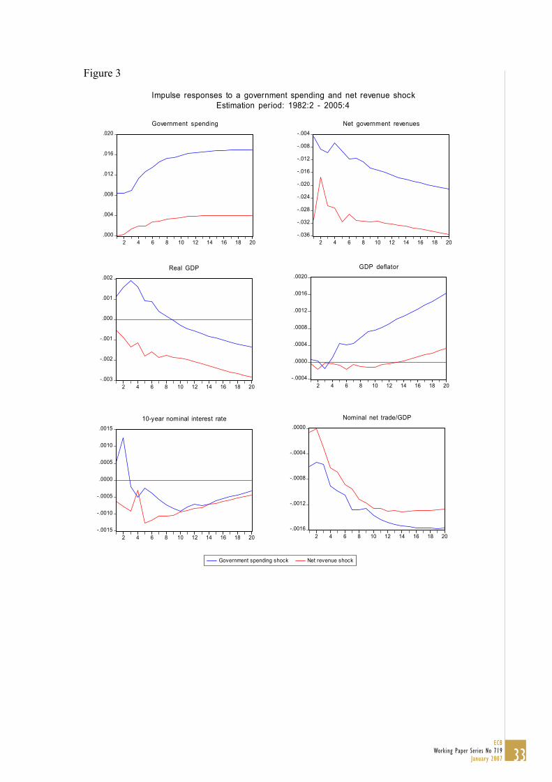
{Insert Figure 3}
Figure 3 shows the response of each of the variables to the government spending and
net revenue shock. A few results are worth highlighting. First, a one-standard
deviation positive government spending shock increases output in the short run by
about 0.1 to 0.2%. This effect is marginally significant. In contrast, a reduction in
taxes does not appear to have a significant impact on output, and if anything leads to a
fall in output. While in particular the latter result is quite surprising, it is consistent
with the results of Perotti (2005), who finds that the output effects of government
spending are typically larger than those of a comparable change in revenues in five
OECD countries (including the US). Perotti (2005) also finds that in general the 20 This is the benchmark specification in Perotti (2005). As in this contribution, our results are broadly similar when we invert the ordering of spending and revenues.
17ECB
Working Paper Series No 719January 2007
output effects of a government spending shock have fallen significantly since the
early 1980s. Second, both an increase in spending and a tax cut have a negative effect
on the net trade/GDP ratio. In the case of a positive spending shock, we observe an
immediate significant negative impact on the external balance. The associated
multiplier is in the order of 0.30 to 0.40 and thus somewhat higher than the one found
in Bussiere et al. (2005). For a tax shock the negative impact on net trade takes longer
to materialise and is also less significant. In this case the multiplier ranges from 0.01
for immediate impact to 0.30 for impact after 12 quarters.21
In sum, overall we find a significant role of the deterioration of fiscal balances for the
deterioration of the net trade balance. The quantitative relevance of fiscal policy
shocks for the most recent deterioration of the current account will be examined in
Section 3.
2.3. Monetary policy Finally, we investigate the role of monetary policy in the developments of the current
account. One popular story is that loose monetary policy following the collapse of the
dot-com asset price bubble, the resulting recession and fears of deflation has led to
low short and long-term interest rates and rising house prices.22 This in turn has
stimulated domestic demand leading to a rise in imports and a deterioration of the
terms of trade, both contributing to a rise in the nominal trade balance deficit. Indeed,
as inflation has declined since the early 1980s, also nominal short and long-term
interest rates have fallen considerably over the last two decades. More importantly,
real short-term interest rates have been significantly negative in the period 2001-2004.
However, in order to asses whether monetary policy has been exceptionally loose, one
needs to control for the normal policy response to changes in inflation and real
economic activity. This is exactly what the large VAR literature on estimating the
21 To obtain fiscal multiplier, the shock was expressed as a percentage point change in government spending/GDP (net revenue/GDP) by multiplying the shock with average spending/GDP (net revenue/GDP) ratio. For our sample period, average shares are 0.19 for spending/GDP and 0.14 for net revenues/GDP. 22 See, for example, Gros, Mayer and Ubide (2006).
18ECB Working Paper Series No 719January 2007
effects of monetary policy on the US economy has tried to do.23 In this section, we
follow the recent work by Kim (2001), who builds on this literature to analyse the
effects of US monetary policy shocks on the trade balance and other international
variables. More specifically, Kim (2001) estimates a small-scale VAR in real GDP,
the GDP deflator, the federal funds rate and a commodity price index over the period
1974-1996. Following Christiano, Eichenbaum and Evans (1999), he identifies
monetary policy shocks by assuming that they have no contemporaneous effects on
output, inflation and commodity prices. Commodity prices are included to alleviate
the so-called price puzzle, the common finding that prices rise for a while following
an unexpected interest rate increase. A similar VAR is used by Boivin and Giannoni
(2005) to investigate whether monetary policy has become more effective in the post-
1982 period. Using this VAR, Kim (2001) and Boivin and Giannoni (2005) show that
a rise in the federal funds rate leads to a hump-shaped fall in output and a much more
gradual decline in prices. Kim (2001) then investigates the effects of a US monetary
policy shock on the trade balance and foreign output. He finds that an expansionary
monetary policy shock worsens the US real trade balance in about a year and leads to
a terms-of-trade deterioration as the dollar exchange rate depreciates. Overall, this
contributes to a significant deterioration of the nominal trade balance in the short to
medium-run.
In analogy with the previous sections, we update the findings of Kim (2001) by
estimating a similar VAR and using a similar identification strategy over the sample
period 1982:2 till 2005:4. Apart from the different sample period, there are two main
differences in the specification of the VAR. First, we leave out the commodity price
index, as over this sample the inclusion of commodity prices did not improve the
estimated effects of the policy shock very much (either in terms of sharpening the
confidence bands or alleviating the price puzzle). Second, we introduce real GDP and
the GDP deflator in log first differences (rather than in log levels) anticipating the
specification of the large-scale VAR in the next Section. Neither of these changes has
a material impact on the estimated impulse responses. Finally, as with the other VARs
discussed in this Section, the net trade/GDP ratio (NX) is introduced in first
differences and it is assumed that the monetary policy shock can have an immediate
23 One of the classic references is Christiano, Eichenbaum and Evans (1999).
19ECB
Working Paper Series No 719January 2007
impact on net trade/GDP ratio, but that policy does not immediately respond to
changes in the net trade ratio. Precisely, in this case Yt is defined as:
⎥⎥⎥
⎦
⎤
⎢⎢⎢
⎣
⎡
∆=
t
t
t
t
NXiX
Y ,
where Xt includes the growth rates of real GDP and GDP deflator, and it is the federal
fund rate. As before, in order to recover the monetary policy shock we need to
appropriately restrict matrix C in order to be able to recover its third column,
describing the effect of a monetary policy shock on the VAR variables. Following
Christiano, Eichenbaum and Evans (1999) and Kim (2001), without loss of generality
we assume that C has a recursive structure, so that the column of interest can be
recovered from the third column of the Choleski factor of Σ . The monetary policy
shock is then effectively identified as the residual from a regression of the policy
instrument it over contemporaneous and lagged values of Xt and only lagged values of
net trade and itself, controlling this way for the normal policy response to changes in
inflation and real economic activity. This means that systematic monetary policy is
assumed to react within the same quarter to observed values of GDP growth and
inflation; for instance, increases in the nominal rate which only reflect increases in
current and past inflation will not be attributed to exogenous changes in the monetary
policy stance.
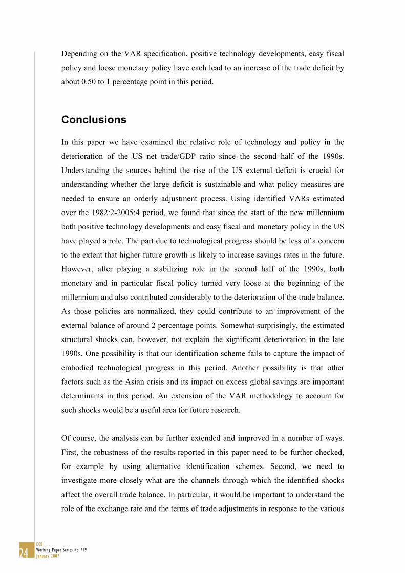
{Insert Figure 4}
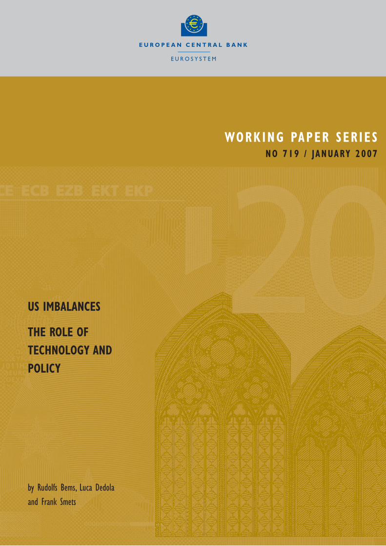
Figure 4 shows the estimated impulse responses of the federal funds rate, the GDP
deflator, real GDP and the net trade/GDP ratio to a monetary policy shock over the
recent sample. The results confirm the findings of Kim (2001) and Boivin and
Giannoni (2005): An unexpected temporary tightening of the federal funds rate by 50
basis points leads to a hump-shaped decline in real GDP of maximally 30 to 40 basis
points and a very gradual (but not significant) decline in the GDP deflator. More
importantly for our purposes, the nominal net trade/GDP ratio improves significantly
in the second year following the shock. According to these estimates, a 50 basis point
policy easing leads to a maximum deterioration of the net trade/GDP ratio of 0.2
percentage points after two years. These multipliers are both statistically and
economically significant and appear to be quite robust with respect to adding
20ECB Working Paper Series No 719January 2007
additional variables. It will therefore be interesting to see how much the monetary
policy easing of the early millennium can contribute to the deterioration of the trade
balance during that period. This will be discussed in the next section.24
3. The contribution of technology and policy to US current account developments In the previous section, we analyzed the effects of technology and policy shocks on
the trade balance in separate VARs by following and extending the existing VAR
literature. This allowed us to keep the size of the VARs relatively small, which is
important given the relatively limited sample size. However, in order to assess the
relative contributions of technology versus policy shocks in driving external trade and
current account developments, it is crucial to put the various shocks into one VAR.
This is what we do in this Section. In order to maintain enough degrees of freedom,
we restrict the number of variables in the VAR to eight and the number of identified
shocks to four. First, the price of equipment is included in order to identify the
embodied technology shock. Second, we use non-farm business sector labour
productivity to identify the multi-factor productivity shock. As before, both
technology shocks are identified using long-run restrictions. Third, in line with the
twin-deficit hypothesis we combine the government spending and revenue shock into
one government deficit shock by constructing an adjusted government deficit measure
which takes into account the short-run automatic multipliers of the deficit with respect
to output and inflation. Fourth, monetary policy developments are captured by the
federal funds rate. As before, both policy shocks are identified using short-run
restrictions. In addition to the four variables that are necessary to identify the four
shocks, we add real private consumption and real private investment (which together
form domestic private absorption), the change in the GDP deflator and the net
external trade/GDP ratio. More details regarding the identification scheme are given
in the appendix.
24 Adding financial variables to the VAR, we also found that the long-term rate does significantly rise in response to the monetary policy tightening. The effect of a 50 basis point increase is to raise the 10-year bond yield temporarily by 10 basis points. Moreover, the policy tightening also leads to a fall in real house prices by about 2 percent. However, this effect is only significant at the 10% confidence level.
21ECB
Working Paper Series No 719January 2007
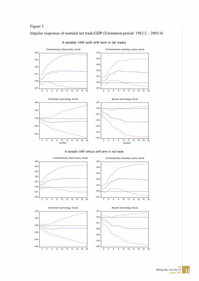
{Insert Figure 5}
Figure 5 reports the impulse responses of the nominal net trade/GDP ratio to each of
the four identified shocks (together with two standard deviation confidence bands) in
two versions of the 8-variable VAR. The upper panel is based on a VAR that includes
a drift term (or constant) in the equation for the change in the net trade/GDP ratio.
This drift term captures the secular fall in the net trade/GDP ratio over the sample
period by about 0.20 percentage points per year. As the constant is not significantly
different from zero, we also report the results of a similar VAR without such a drift
term in the lower panel of Figure 5. Such a VAR allows us to investigate to what
extent the four structural shocks can contribute to the secular fall in the net trade/GDP
ratio over the full sample. It is easy to verify that in both cases the overall effects of
the four structural shocks on net trade are very similar to what we found in the more
specialized VARs discussed in Section 2. This shows that the estimated effects are
quite robust with respect to the choice of variables that are included in the VAR. As
before, it turns out that a one-standard deviation multi-factor productivity and
monetary policy shock have the largest and most significant effect on the net
trade/GDP ratio.
{Insert Table 2}
How much of the swings in the US external trade balance over the past two decades
can the four structural shocks account for? Table 2 gives the contribution of each of
the shocks to the forecast error variance of changes in the net trade/GDP ratio at
various horizons. It turns out that the fiscal, monetary policy and technology shocks
each explain between 8 and 12 percent of the forecast variance at business cycle
frequencies. Figure 6 plots the actual net trade/GDP ratio as well as the joint
contribution of the four shocks and the baseline over the full sample period in the
VARs with and without a drift term in net trade. This figure also plots the contribution
of the four shocks to the growth of domestic absorption, the inflation rate and the
federal funds rate. Comparing the contribution to net trade in both VARs (Figure 6), it
is clear that the VAR with a drift term is better able to account for the secular fall in
net trade over the sample period. However, it is also clear that the main failure of the
VAR without a drift term to account for this trend is located in the 1990s. In fact, it is
22ECB Working Paper Series No 719January 2007
worth distinguishing three episodes, which are analysed in more detail in Figures 7a
and 7b. The first episode covers the 1980s. In this period, the four structural shocks
are able to explain the drop in the net trade balance in the early 1980s and the
subsequent increase in the second half of the 1980s and the beginning of the 1990s.
Looking at the contribution of the shocks separately (Figure 7a,b), it appears that
technology developments and to a lesser extent a reversal of loose fiscal policy have
contributed to a return of the net trade deficit to almost balance. The second episode
covers most of the 1990s. In contrast to the 1980s, the structural shocks can not
explain the large deterioration of the net trade balance in the 1990s (in particular the
three percentage point deterioration since 1997). It is interesting to see that in this
period, both inflation and the nominal interest rate are overpredicted. Moreover, the
structural shocks can not explain the investment boom associated with the dot-com
bubble in the late 1990s either, the period with the most rapid deterioration of net
trade in the United States. As discussed in the introduction, a number of other not
necessarily US driven developments have been proposed to explain the growing
imbalances. Three of those are worth mentioning. First, following the Asian crisis in
1997-1998, a number of Asian countries such as Korea, Malaysia, Thailand and
Indonesia experienced a sharp and persistent drop in investment rates, coupled with
temporarily high savings rates. These developments coincided with a build up of
official reserves as of 1999. These changes coincide with the emergence of a large
gap between actual net trade developments in the US and the part explained by our
US shocks (see Figure 7) and therefore may explain part of this gap. Second, the rapid
accumulation of reserves in China following strong growth in exports under its
mercantilist policy only took off in 2001 and therefore is unlikely to explain what
happened in the second subperiod. Finally, most recently more emphasis has been put
on the recycling of petrodollars as a factor behind the growing global imbalances.
However, also this factor only became relevant after 1999, suggesting that it can not
explain the gap in Figure 7 in the 1997-2000 period.
{Insert Figure 6}
{Insert Figure 7}
Finally, turning to the most recent period since 2000, it turns out that the three types
of shocks have all contributed to the further deterioration of the net trade/GDP ratio.
23ECB
Working Paper Series No 719January 2007
Depending on the VAR specification, positive technology developments, easy fiscal
policy and loose monetary policy have each lead to an increase of the trade deficit by
about 0.50 to 1 percentage point in this period.
Conclusions In this paper we have examined the relative role of technology and policy in the
deterioration of the US net trade/GDP ratio since the second half of the 1990s.
Understanding the sources behind the rise of the US external deficit is crucial for
understanding whether the large deficit is sustainable and what policy measures are
needed to ensure an orderly adjustment process. Using identified VARs estimated
over the 1982:2-2005:4 period, we found that since the start of the new millennium
both positive technology developments and easy fiscal and monetary policy in the US
have played a role. The part due to technological progress should be less of a concern
to the extent that higher future growth is likely to increase savings rates in the future.
However, after playing a stabilizing role in the second half of the 1990s, both
monetary and in particular fiscal policy turned very loose at the beginning of the
millennium and also contributed considerably to the deterioration of the trade balance.
As those policies are normalized, they could contribute to an improvement of the
external balance of around 2 percentage points. Somewhat surprisingly, the estimated
structural shocks can, however, not explain the significant deterioration in the late
1990s. One possibility is that our identification scheme fails to capture the impact of
embodied technological progress in this period. Another possibility is that other
factors such as the Asian crisis and its impact on excess global savings are important
determinants in this period. An extension of the VAR methodology to account for
such shocks would be a useful area for future research.
Of course, the analysis can be further extended and improved in a number of ways.
First, the robustness of the results reported in this paper need to be further checked,
for example by using alternative identification schemes. Second, we need to
investigate more closely what are the channels through which the identified shocks
affect the overall trade balance. In particular, it would be important to understand the
role of the exchange rate and the terms of trade adjustments in response to the various
24ECB Working Paper Series No 719January 2007
shocks. We also need to analyze to what extent the estimated effects are consistent
with modern intertemporal open-economy macro models in order to increase our
confidence in the estimated effects.
Appendix: The identification scheme of the VAR estimated in Section 3 In Section 3 we estimated the following reduced form VAR:
( )( )
.
loglog
,...
,',1
21
1
⎥⎥⎥⎥⎥⎥⎥
⎦
⎤
⎢⎢⎢⎢⎢⎢⎢
⎣
⎡
∆
∆∆∆
=
+++≡
Σ=+=−
−
t
t
t
t
t
t
t
ttttt
NXiX
BDzp
Y
LBLBBLB
uEuuYLBY
First, the price of equipment pt is included in order to identify the embodied
technology shock. Second, we use non-farm business sector labour productivity zt to
identify the multi-factor productivity shock. Third, in line with the twin-deficit
hypothesis we combine the government spending and revenue shock into one
government deficit shock by constructing an adjusted government deficit measure
which takes into account the short-run automatic multipliers of the deficit with respect
to output and inflation, BDt. Fourth, monetary policy developments are captured by
the federal funds rate it. In addition to the four variables that are necessary to identify
the four shocks, we include in vector Xt the growth rate of real private consumption
and real private investment (which together form domestic private absorption) and the
change in the GDP deflator, and finally the net external trade/GDP ratio.
As before, both technology shocks are identified using long-run restrictions, while
both policy shocks are identified using short-run restrictions. Concretely, we proceed
in the following way. First, in order to identify the two technology shocks we estimate
the corresponding two columns of the C matrix by a straightforward generalization of
the procedure described in Section 2.1. The two long-run restrictions imply that the
long-run responses of the above system satisfy:
25ECB
Working Paper Series No 719January 2007
( )[ ]
⎥⎥⎥⎥⎥
⎦
⎤
⎢⎢⎢⎢⎢
⎣
⎡
=−≡Ρ
−−−−
−
−−
)2()2(,.
1)2(2,
1)2(1,
)2(121
)2(111 0
00
1
NxNZ
xNZ
xNZ
Nxzz
Nxp
RRR
rr
r
CBI ,
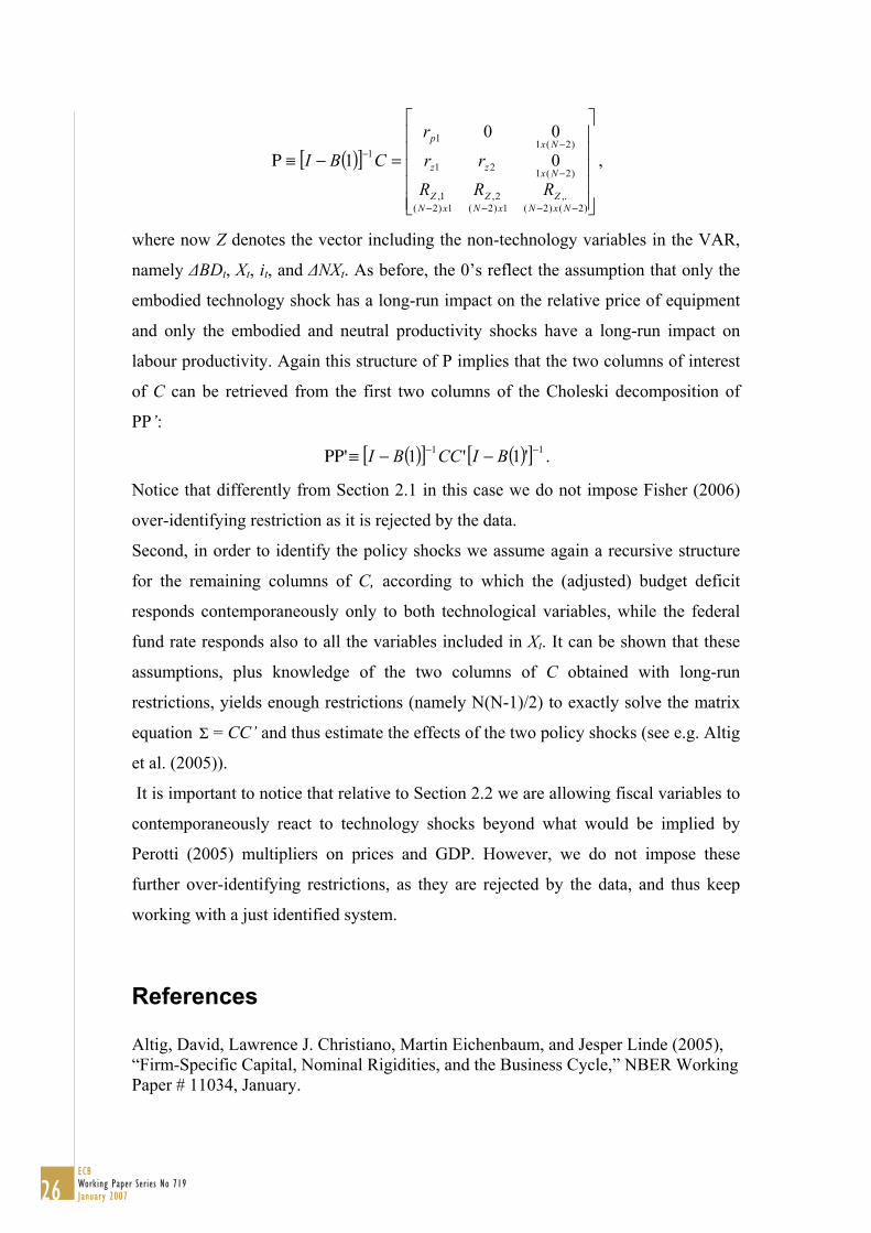
where now Z denotes the vector including the non-technology variables in the VAR,
namely ∆BDt, Xt, it, and ∆NXt. As before, the 0’s reflect the assumption that only the
embodied technology shock has a long-run impact on the relative price of equipment
and only the embodied and neutral productivity shocks have a long-run impact on
labour productivity. Again this structure of P implies that the two columns of interest
of C can be retrieved from the first two columns of the Choleski decomposition of
PP’:
( )[ ] ( )[ ] 11 '1'1' −− −−≡ΡΡ BICCBI .
Notice that differently from Section 2.1 in this case we do not impose Fisher (2006)
over-identifying restriction as it is rejected by the data.
Second, in order to identify the policy shocks we assume again a recursive structure
for the remaining columns of C, according to which the (adjusted) budget deficit
responds contemporaneously only to both technological variables, while the federal
fund rate responds also to all the variables included in Xt. It can be shown that these
assumptions, plus knowledge of the two columns of C obtained with long-run
restrictions, yields enough restrictions (namely N(N-1)/2) to exactly solve the matrix
equation Σ = CC’ and thus estimate the effects of the two policy shocks (see e.g. Altig
et al. (2005)).
It is important to notice that relative to Section 2.2 we are allowing fiscal variables to
contemporaneously react to technology shocks beyond what would be implied by
Perotti (2005) multipliers on prices and GDP. However, we do not impose these
further over-identifying restrictions, as they are rejected by the data, and thus keep
working with a just identified system.
References Altig, David, Lawrence J. Christiano, Martin Eichenbaum, and Jesper Linde (2005), “Firm-Specific Capital, Nominal Rigidities, and the Business Cycle,” NBER Working Paper # 11034, January.
26ECB Working Paper Series No 719January 2007
Backus, David, Espen Henriksen, Frederic Lambert and Chris Telmer (2006), “Current Account Fact and Fiction,” mimeo. Bank of International Settlement (2004), 74th Annual Report, Basel, June. Bernanke, Ben (2005), “The worldwide saving glut and the US current account deficit,” remarks at the Sandridge and Homer Jones Lectures, March and April. Blanchard, Olivier and Roberto Perotti (2002), “An Empirical Characterization of the Dynamic Effects of Changes in Government Spending and Taxes on Output,” Quarterly Journal of Economics, 117(4), 1329-1368. Boivin, Jean and Marc P. Giannoni (2005), “Has Monetary Policy Become More Effective?” The Review of Economics and Statistics, Forthcoming. Bussière, Matthieu, Marcel Fratzscher and Gernot J. Müller (2005), “Productivity Shocks, Budget Deficits and the Current Account,” ECB Working Paper 509. Caballero, R., E. Farhi, and P. Gourinchas (2005), “An Equilibrium Model of `Global Imbalances' and Low Interest Rates,” mimeo. Christiano, Lawrence J., Eichenbaum, Martin, and Charles L. Evans (1999), “Monetary Policy Shocks: What Have We Learned and To What End?” Handbook of Macroeconomics, eds. J.B. Taylor and M. Woodford, Amsterdam: Elsevier, pp. 65-148. Clarida, Richard, Jordi Gali and Mark Gertler (2000), “Monetary Policy Rules and Macroeconomic Stability: Evidence and Some Theory,” Quarterly Journal of Economics, vol. CXV, issue 1, 147-180, 2000. Corsetti, Giancarlo (2005), “Global Imbalances,” mimeo. Corsetti, Giancarlo, Luca Dedola and Sylvain Leduc (2006), “Productivity, External Balance and Exchange Rates: Evidence on the Transmission Mechanism among G7 Countries,” CEPR Discussion Paper 5853. Corsetti, Giancarlo and Gernot J. Müller (2006), “Twin Deficits: Squaring Theory, Evidence and Common Sense,” Economic Policy, Forthcoming. De Walque, Gregory, Frank Smets and Raf Wouters (2005), “An Estimated Two-Country DSGE Model for the Euro Area and the US Economy”, mimeo. Dedola, Luca and Stefano Neri (2005), “What does a technology shock do? A VAR analysis with model-based sign restrictions,” Journal of Monetary Economics, Forthcoming. Dooley, M., D. Folkerts-Landau and P. Garber (2005), “Direct Investment, Rising Real Wages And The Absorption Of Excess Labor In The Periphery,” in R. Clarida (ed.) "G7 Current Account Imbalances: Sustainability and Adjustment" NBER.
27ECB
Working Paper Series No 719January 2007
Engel, C., and J. Rogers (2006), “The U.S. Current Account Deficit and the Expected Share of World Output,” Journal of Monetary Economics, Forthcoming. Erceg, Christopher J., Guerrieri, Luca and Chistopher Gust (2005), “Expansionary Fiscal Shocks and the Trade Deficit,” International Finance, Vol.8, (December), pp. 363-397. Fisher, Jonas (2006), "The Dynamic Effects of Neutral and Investment-Specific Technology Shocks," Journal of Political Economy, Vol. 114, no. 3, June.. Francis, Neville and Valerie Ramey (2005), "Is the Technology-Driven Real Business Cycle Hypothesis Dead? Shocks and Aggregate Fluctuations Revisited," Journal of Monetary Economics, vol. 52, pp. 1379---99. Gali, Jordi (1999), “Technology, Employment and the Business Cycle: Do Technology Shocks Explain Aggregate Fluctuations?” American Economic Review, 89, 249-271. Gali, Jordi, J. David Lopez-Salido and Javier Valles (2003), “Technology Shocks and Monetary Policy: Assessing the Fed's Performance,” NBER Working Papers 8768. Gali, Jordi and Pau Rabanal (2004), “Technology Shocks and Aggregate Fluctuations: How Well Does the RBC Model Fit Postwar U.S. Data?” NBER Macroeconomics Annual, 2004. Glick, Reuven and Kenneth Rogoff (1995), “Global versus Country-Specific Productivity Shocks and the Current Account,” Journal of Monetary Economics,” 35 (1995), 159-192. Gros, Daniel, Thomas Mayer and Angel Ubide (2006), “A World Out of Balance?” Special Report of the CEPS Macroeconomic Policy Group, Brussels. Hausmann R., and F., Sturzenegger (2005), “US and Global Imbalances: Can Dark matter Prevent a Big Bang?” mimeo. Hunt, Benjamin and Alessandro Rebucci (2005), “The US Dollar and the Trade Deficit: What Accounts for the Late 1990s?” International Finance 8 (3), 399-434. International Monetary Fund (2005), World Economic Outlook, Washington, DC, April. International Monetary Fund (2006), World Economic Outlook, Washington, DC, April. Kim, Soyoung (2001), “International transmission of U.S. monetary policy shocks: Evidence from VAR's,” Journal of Monetary Economics, 48, 339-372. Kim, Soyoung and Nouriel Roubini (2004), “Twin Deficits or Twin Divergence? Fiscal Policy, Current Account, and Real Exchange Rate in the US,” mimeo.
28ECB Working Paper Series No 719January 2007
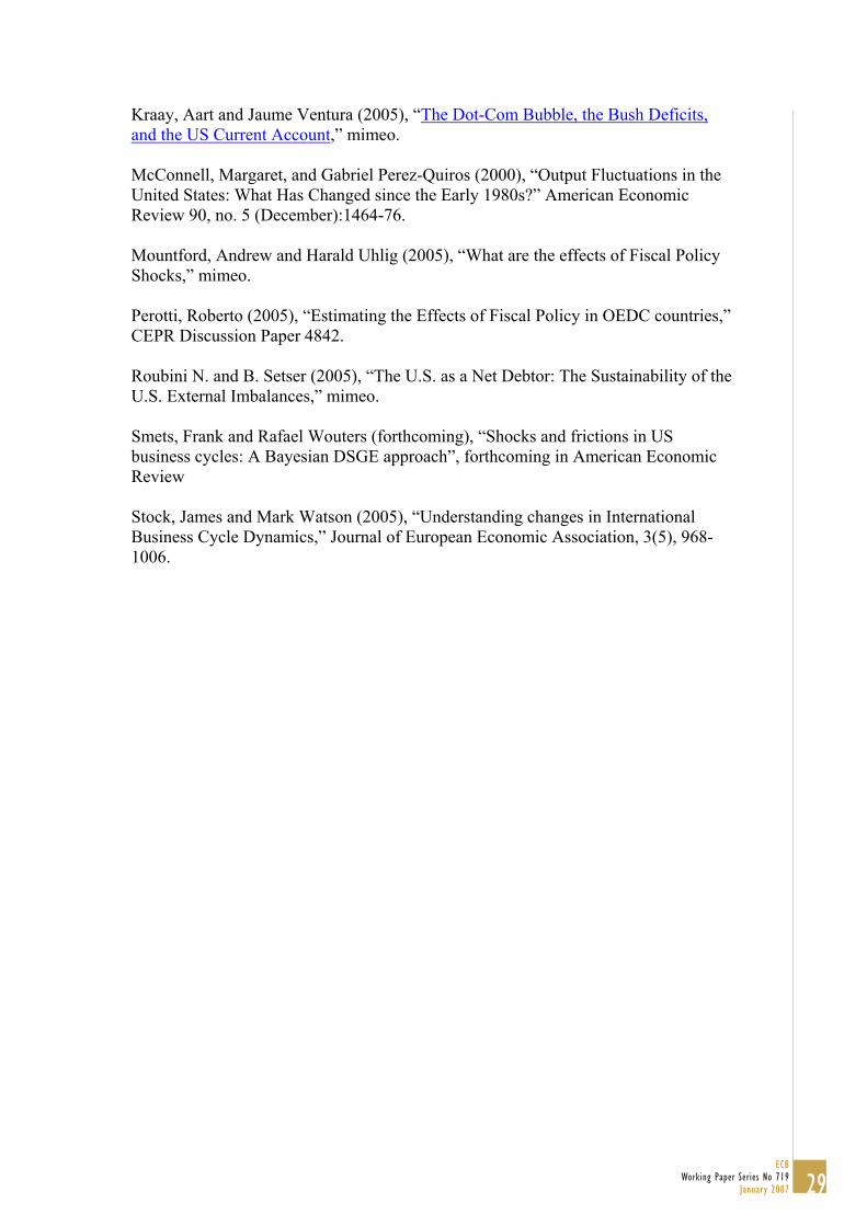
Kraay, Aart and Jaume Ventura (2005), “The Dot-Com Bubble, the Bush Deficits, and the US Current Account,” mimeo. McConnell, Margaret, and Gabriel Perez-Quiros (2000), “Output Fluctuations in the United States: What Has Changed since the Early 1980s?” American Economic Review 90, no. 5 (December):1464-76. Mountford, Andrew and Harald Uhlig (2005), “What are the effects of Fiscal Policy Shocks,” mimeo. Perotti, Roberto (2005), “Estimating the Effects of Fiscal Policy in OEDC countries,” CEPR Discussion Paper 4842. Roubini N. and B. Setser (2005), “The U.S. as a Net Debtor: The Sustainability of the U.S. External Imbalances,” mimeo. Smets, Frank and Rafael Wouters (forthcoming), “Shocks and frictions in US business cycles: A Bayesian DSGE approach”, forthcoming in American Economic Review Stock, James and Mark Watson (2005), “Understanding changes in International Business Cycle Dynamics,” Journal of European Economic Association, 3(5), 968-1006.
29ECB
Working Paper Series No 719January 2007
30
ECB Working Paper Series No 719January 2007
Table 1
Table 2: Contribution of the four shocks to the variance of changes in net trade/GDP
(a) 8 variable VAR with drift term
Forecast variance at indicated horizon Type of shock 1 4 8 12 20 Fiscal policy 4.9 9.8 8.3 8.3 8.3 Embodied technology 4.0 4.7 4.8 5.2 5.2 Neutral technology 1.4 5.2 6.5 7.3 7.2 Monetary policy 4.1 9.8 10.1 10.0 10.0
(b) 8 variable VAR without drift term
Forecast variance at indicated horizon Type of shock 1 4 8 12 20 Fiscal policy 6.3 10.4 9.0 8.9 8.9 Embodied technology 2.9 4.1 4.2 4.6 4.6 Neutral technology 0.0 4.2 5.4 6.0 5.9 Monetary policy 4.4 10.5 10.6 10.3 10.3
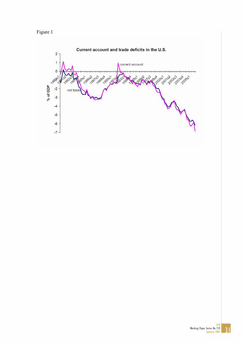
Figure 1
31ECB
Working Paper Series No 719January 2007
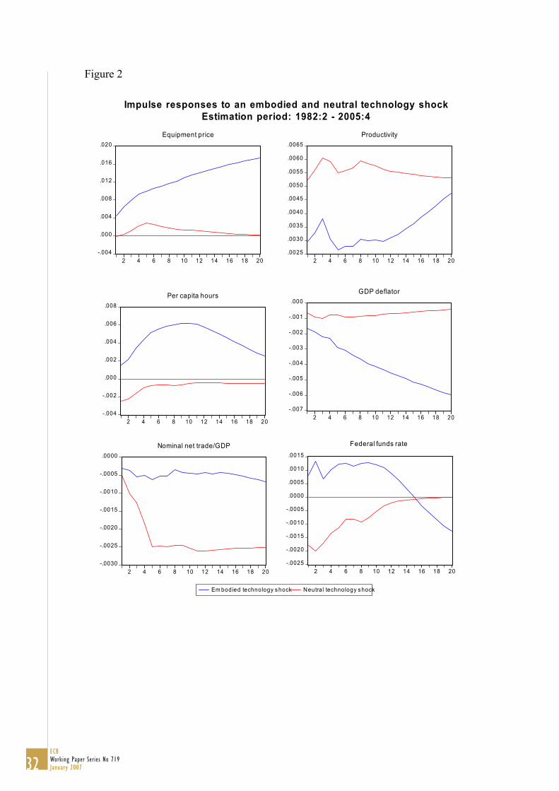
Figure 2
-.004
.000
.004
.008
.012
.016
.020
2 4 6 8 10 12 14 16 18 20
Em bodied technology s hock Neutral technology s hock
Equipment price
.0025
.0030
.0035
.0040
.0045
.0050
.0055
.0060
.0065
2 4 6 8 10 12 14 16 18 20
Productivity
-.007
-.006
-.005
-.004
-.003
-.002
-.001
.000
2 4 6 8 10 12 14 16 18 20
GDP deflator
-.0030
-.0025
-.0020
-.0015
-.0010
-.0005
.0000
2 4 6 8 10 12 14 16 18 20
Nominal net trade/GDP
-.004
-.002
.000
.002
.004
.006
.008
2 4 6 8 10 12 14 16 18 20
Per capita hours
-.0025
-.0020
-.0015
-.0010
-.0005
.0000
.0005
.0010
.0015
2 4 6 8 10 12 14 16 18 20
Federal funds rate
Impulse responses to an embodied and neutral technology shockEstimation period: 1982:2 - 2005:4
32ECB Working Paper Series No 719January 2007
.000
.004
.008
.012
.016
.020
2 4 6 8 10 12 14 16 18 20
Government spending shock Net revenue shock
Government spending
-.036
-.032
-.028
-.024
-.020
-.016
-.012
-.008
-.004
2 4 6 8 10 12 14 16 18 20
Net government revenues
-.003
-.002
-.001
.000
.001
.002
2 4 6 8 10 12 14 16 18 20
Real GDP
-.0004
.0000
.0004
.0008
.0012
.0016
.0020
2 4 6 8 10 12 14 16 18 20
GDP deflator
-.0016
-.0012
-.0008
-.0004
.0000
2 4 6 8 10 12 14 16 18 20
Nominal net trade/GDP
-.0015
-.0010
-.0005
.0000
.0005
.0010
.0015
2 4 6 8 10 12 14 16 18 20
10-year nominal interest rate
Impulse responses to a government spending and net revenue shockEstimation period: 1982:2 - 2005:4
33ECB
Working Paper Series No 719January 2007
Figure 3
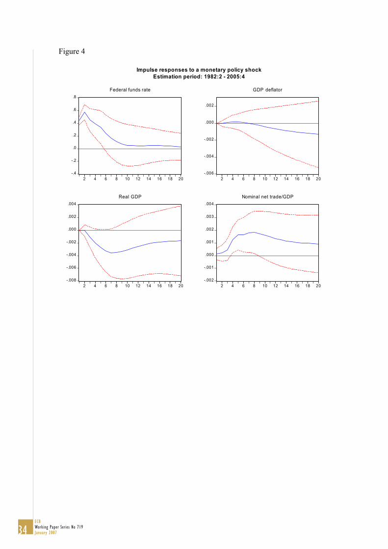
Figure 4
-.4
-.2
.0
.2
.4
.6
.8
2 4 6 8 10 12 14 16 18 20
Federal funds rate
-.006
-.004
-.002
.000
.002
2 4 6 8 10 12 14 16 18 20
GDP deflator
-.008
-.006
-.004
-.002
.000
.002
.004
2 4 6 8 10 12 14 16 18 20
Real GDP
-.002
-.001
.000
.001
.002
.003
.004
2 4 6 8 10 12 14 16 18 20
Nominal net trade/GDP
Impulse responses to a monetary policy shockEstimation period: 1982:2 - 2005:4
34ECB Working Paper Series No 719January 2007
35
ECB Working Paper Series No 719
January 2007
Figure 5
Impulse responses of nominal net trade/GDP (Estimation period: 1982:2 – 2005:4)
-.001
.000
.001
.002
.003
.004
2 4 6 8 10 12 14 16 18 20
Contractionary fiscal policy shock
-.001
.000
.001
.002
.003
.004
.005
2 4 6 8 10 12 14 16 18 20
Contractionary monetary policy shock
-.004
-.002
.000
.002
.004
2 4 6 8 10 12 14 16 18 20
Embodied technology shock
-.005
-.004
-.003
-.002
-.001
.000
.001
2 4 6 8 10 12 14 16 18 20
Neutral technology shock
8-variable VAR (with drift term in net trade)
Quarters Quarters
-.002
-.001
.000
.001
.002
.003
.004
.005
2 4 6 8 10 12 14 16 18 20
Contractionary fiscal policy shock
-.001
.000
.001
.002
.003
.004
.005
2 4 6 8 10 12 14 16 18 20
Contractionary monetary policy shock
-.006
-.004
-.002
.000
.002
.004
2 4 6 8 10 12 14 16 18 20
Embodied technology shock
-.005
-.004
-.003
-.002
-.001
.000
.001
2 4 6 8 10 12 14 16 18 20
Neutral technology shock
8-variable VAR without drift term in net trade
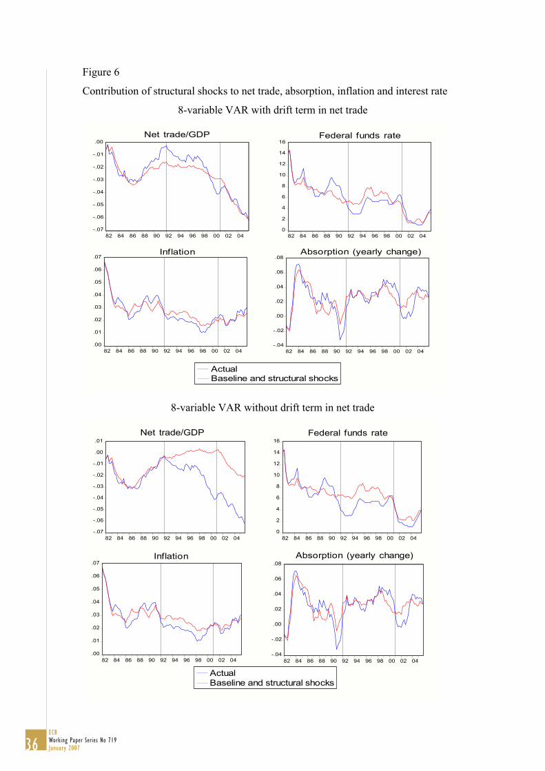
Figure 6
Contribution of structural shocks to net trade, absorption, inflation and interest rate
8-variable VAR with drift term in net trade
-.07
-.06
-.05
-.04
-.03
-.02
-.01
.00
82 84 86 88 90 92 94 96 98 00 02 04
ActualBaseline and structural shocks
Net trade/GDP
0
2
4
6
8
10
12
14
16
82 84 86 88 90 92 94 96 98 00 02 04
Federal funds rate
.00
.01
.02
.03
.04
.05
.06
.07
82 84 86 88 90 92 94 96 98 00 02 04-.04
-.02
.00
.02
.04
.06
.08
82 84 86 88 90 92 94 96 98 00 02 04
Inflation Absorption (yearly change)
8-variable VAR without drift term in net trade
-.07
-.06
-.05
-.04
-.03
-.02
-.01
.00
.01
82 84 86 88 90 92 94 96 98 00 02 04
ActualBaseline and structural shocks
0
2
4
6
8
10
12
14
16
82 84 86 88 90 92 94 96 98 00 02 04
.00
.01
.02
.03
.04
.05
.06
.07
82 84 86 88 90 92 94 96 98 00 02 04-.04
-.02
.00
.02
.04
.06
.08
82 84 86 88 90 92 94 96 98 00 02 04
Net trade/GDP Federal funds rate
Inflation Absorption (yearly change)
36ECB Working Paper Series No 719January 2007
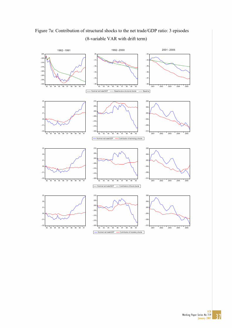
Figure 7a: Contribution of structural shocks to the net trade/GDP ratio: 3 episodes
(8-variable VAR with drift term)
-.035
-.030
-.025
-.020
-.015
-.010
-.005
.000
82 83 84 85 86 87 88 89 90 91
Nominal net trade/GDP Baseline plus structural shocks Baseline
-.05
-.04
-.03
-.02
-.01
.00
92 93 94 95 96 97 98 99 00-.08
-.07
-.06
-.05
-.04
-.03
2001 2002 2003 2004 2005
-.02
-.01
.00
.01
.02
.03
82 83 84 85 86 87 88 89 90 91
Nominal net trade/GDP Contribution of technology shocks
-.020
-.015
-.010
-.005
.000
.005
.010
92 93 94 95 96 97 98 99 00-.012
-.008
-.004
.000
.004
.008
2001 2002 2003 2004 2005
-.02
-.01
.00
.01
.02
.03
82 83 84 85 86 87 88 89 90 91
Nominal net trade/GDP Contribution of fiscal shocks
-.020
-.015
-.010
-.005
.000
.005
.010
92 93 94 95 96 97 98 99 00-.012
-.008
-.004
.000
.004
.008
2001 2002 2003 2004 2005
-.02
-.01
.00
.01
.02
.03
82 83 84 85 86 87 88 89 90 91
Nominal net trade/GDP Contribution of monetary shocks
-.020
-.015
-.010
-.005
.000
.005
.010
92 93 94 95 96 97 98 99 00-.012
-.008
-.004
.000
.004
.008
2001 2002 2003 2004 2005
1982 - 1991 1992 - 2000 2001 - 2005
37ECB
Working Paper Series No 719January 2007
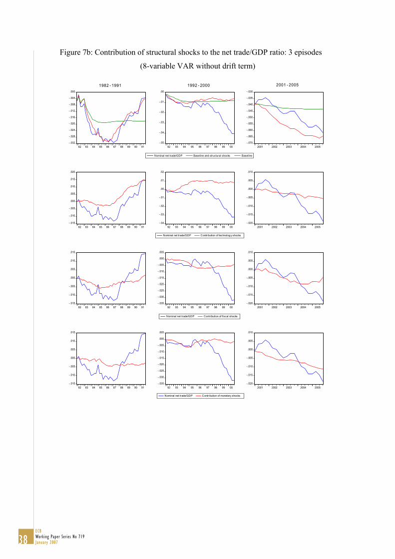
Figure 7b: Contribution of structural shocks to the net trade/GDP ratio: 3 episodes
(8-variable VAR without drift term)
-.032
-.028
-.024
-.020
-.016
-.012
-.008
-.004
.000
82 83 84 85 86 87 88 89 90 91
Nominal net trade/GDP Baseline and structural shocks Baseline
-.05
-.04
-.03
-.02
-.01
.00
92 93 94 95 96 97 98 99 00-.070
-.065
-.060
-.055
-.050
-.045
-.040
-.035
-.030
2001 2002 2003 2004 2005
-.015
-.010
-.005
.000
.005
.010
.015
.020
82 83 84 85 86 87 88 89 90 91
Nominal net trade/GDP Contribution of technology shocks
-.04
-.03
-.02
-.01
.00
.01
.02
92 93 94 95 96 97 98 99 00-.020
-.015
-.010
-.005
.000
.005
.010
2001 2002 2003 2004 2005
-.015
-.010
-.005
.000
.005
.010
.015
82 83 84 85 86 87 88 89 90 91
Nominal net trade/GDP Contribution of fiscal shocks
-.035
-.030
-.025
-.020
-.015
-.010
-.005
.000
.005
92 93 94 95 96 97 98 99 00-.020
-.015
-.010
-.005
.000
.005
.010
2001 2002 2003 2004 2005
-.015
-.010
-.005
.000
.005
.010
.015
82 83 84 85 86 87 88 89 90 91
Nominal net trade/GDP Contribution of monetary shocks
-.035
-.030
-.025
-.020
-.015
-.010
-.005
.000
.005
92 93 94 95 96 97 98 99 00-.020
-.015
-.010
-.005
.000
.005
.010
2001 2002 2003 2004 2005
1982 - 1991 1992 - 2000 2001 - 2005
38ECB Working Paper Series No 719January 2007
39ECB
Working Paper Series No 719January 2007
European Central Bank Working Paper Series
For a complete list of Working Papers published by the ECB, please visit the ECB’s website(http://www.ecb.int)
680 “Comparing alternative predictors based on large-panel factor models” by A. D’Agostino and D. Giannone, October 2006.
681 “Regional inflation dynamics within and across euro area countries and a comparison with the US” by G. W. Beck, K. Hubrich and M. Marcellino, October 2006.
682 “Is reversion to PPP in euro exchange rates non-linear?” by B. Schnatz, October 2006.
683 “Financial integration of new EU Member States” by L. Cappiello, B. Gérard, A. Kadareja and S. Manganelli, October 2006.
684 “Inflation dynamics and regime shifts” by J. Lendvai, October 2006.
685 “Home bias in global bond and equity markets: the role of real exchange rate volatility” by M. Fidora, M. Fratzscher and C. Thimann, October 2006
686 “Stale information, shocks and volatility” by R. Gropp and A. Kadareja, October 2006.
687 “Credit growth in Central and Eastern Europe: new (over)shooting stars?” by B. Égert, P. Backé and T. Zumer, October 2006.
688 “Determinants of workers’ remittances: evidence from the European Neighbouring Region” by I. Schiopu and N. Siegfried, October 2006.
689 “The effect of financial development on the investment-cash flow relationship: cross-country evidence from Europe” by B. Becker and J. Sivadasan, October 2006.
690 “Optimal simple monetary policy rules and non-atomistic wage setters in a New-Keynesian framework” by S. Gnocchi, October 2006.
691 “The yield curve as a predictor and emerging economies” by A. Mehl, November 2006.
692 “Bayesian inference in cointegrated VAR models: with applications to the demand for euro area M3” by A. Warne, November 2006.
693 “Evaluating China’s integration in world trade with a gravity model based benchmark” by M. Bussière and B. Schnatz, November 2006.
694 “Optimal currency shares in international reserves: the impact of the euro and the prospects for the dollar” by E. Papaioannou, R. Portes and G. Siourounis, November 2006.
695 “Geography or skills: What explains Fed watchers’ forecast accuracy of US monetary policy?” by H. Berger, M. Ehrmann and M. Fratzscher, November 2006.
696 “What is global excess liquidity, and does it matter?” by R. Rüffer and L. Stracca, November 2006.
697 “How wages change: micro evidence from the International Wage Flexibility Project” by W. T. Dickens, L. Götte, E. L. Groshen, S. Holden, J. Messina, M. E. Schweitzer, J. Turunen, and M. E. Ward, November 2006.
40ECB Working Paper Series No 719January 2007
698 “Optimal monetary policy rules with labor market frictions” by E. Faia, November 2006.
699 “The behaviour of producer prices: some evidence from the French PPI micro data” by E. Gautier, December 2006.
700 “Forecasting using a large number of predictors: Is Bayesian regression a valid alternative toprincipal components?” by C. De Mol, D. Giannone and L. Reichlin, December 2006.
701 “Is there a single frontier in a single European banking market?” by J. W. B. Bos and H. Schmiedel, December 2006.
702 “Comparing financial systems: a structural analysis” by S. Champonnois, December 2006.
703 “Comovements in volatility in the euro money market” by N. Cassola and C. Morana, December 2006.
704 “Are money and consumption additively separable in the euro area? A non-parametric approach” by B. E. Jones and L. Stracca, December 2006.
705 “What does a technology shock do? A VAR analysis with model-based sign restrictions” by L. Dedola and S. Neri, December 2006.
706 “What drives investors’ behaviour in different FX market segments? A VAR-based returndecomposition analysis” by O. Castrén, C. Osbat and M. Sydow, December 2006.
707 “Ramsey monetary policy with labour market frictions” by E. Faia, January 2007.
708 “Regional housing market spillovers in the US: lessons from regional divergences in a common monetary policy setting” by I. Vansteenkiste, January 2007.
709 “Quantifying and sustaining welfare gains from monetary commitment” by P. Levine, P. McAdam and J. Pearlman, January 2007.
710 “Pricing of settlement link services and mergers of central securities depositories” by J. Tapking, January 2007.
711 “What “hides” behind sovereign debt ratings?” by A. Afonso, P. Gomes and P. Rother, January 2007.
M. Lippi and L. Reichlin, January 2007.
January 2007.
714 “The dynamics of bank spreads and financial structure” by R. Gropp, C. Kok Sørensen and J.-D. Lichtenberger, January 2007.
and J.-G. Shen, January 2007.
716 “Adjusting to the euro” by G. Fagan and V. Gaspar, January 2007.
717 “Discretion rather than rules? When is discretionary policy-making better than the timeless perspective?” by S. Sauer, January 2007.
718 “Drift and breaks in labor productivity” by L. Benati, January 2007.
719 “US imbalances: the role of technology and policy” by R. Bems, L. Dedola and F. Smets, January 2007.
712 “Opening the black box: structural factor models with large cross-sections” by M. Forni, D. Giannone,
713 “Balance of payment crises in emerging markets: How early were the “early” warning signals?” by M. Bussière,
715 “Emerging Asia’s growth and integration: How autonomous are business cycles?” by R. Rüffer, M. Sánchez

ISSN 1561081-0
9 7 7 1 5 6 1 0 8 1 0 0 5