Institutional Members: CEPR, NBER and Università Bocconi

WORKING PAPER SERIES

Understanding the Income Gradient in College

Attendance in Mexico: The Role of Heterogeneity in Expected Returns

Katja Maria Kaufmann

Working Paper n. 362

This Version: March 2010

IGIER – Università Bocconi, Via Guglielmo Röntgen 1, 20136 Milano –Italy http://www.igier.unibocconi.it

The opinions expressed in the working papers are those of the authors alone, and not those of the Institute, which takes non institutional policy position, nor those of CEPR, NBER or Università Bocconi.

Understanding the Income Gradient in College Attendance

in Mexico: The Role of Heterogeneity in Expected Returns

Katja Maria Kaufmann∗

Abstract

Differences in college enrollment rates between poor and rich students are a prevalent phe-nomenon, but particularly striking in Latin America. The literature suggests explanations suchas differences in “college preparedness” on the one hand, in that poor students lack skills thatenable them to benefit from college, and “credit constraints” on the other hand. One explana-tion that has been neglected in this analysis consists of differences in information sets betweenthe poor and the rich –for example about career opportunities– translating into different percep-tions of individual returns to college. Data on people’s subjective expectations of returns allowto take this factor into account and to directly address the following identification problem:conditional on their information sets poor people might expect low returns and thus decide notto attend. Or they might face high (unobserved) costs that prevent them from attending de-spite high expected returns. Conventional approaches rely on strong assumptions about people’sinformation sets and about how they form expectations to address this identification problem.

Data on people’s subjective expectations of returns as well as on their schooling decisionsallow me to directly estimate and compare cost distributions of poor and rich individuals. Ifind that poor individuals require significantly higher expected returns to be induced to attendcollege, implying that they face higher costs than individuals with wealthy parents. I then testpredictions of a model of college attendance choice in the presence of credit constraints, usingparental income and wealth as a proxy for the household’s (unobserved) interest rate. I findthat poor individuals with high expected returns are particularly responsive to changes in directcosts, which is consistent with credit constraints playing an important role. Evaluating potentialwelfare implications by applying the Local Instrumental Variables approach of Heckman andVytlacil (2005) to my model, I find that a sizeable fraction of poor individuals would changetheir decision in response to a reduction in direct costs. Individuals at the margin have expectedreturns that are as high or higher than the individuals already attending college, suggesting thatgovernment policies such as fellowship programs could lead to large welfare gains.

JEL-Classification: I21, I22, I38, O15, O16

Keywords: Schooling Choice, Credit Constraints, Subjective Expectations, Marginal Returns to Schooling,Local Instrumental Variables Approach, Mexico.

∗Department of Economics and IGIER, Bocconi University, Address: Via Roentgen 1, 20136 Milano, Italy, e-mail:katja.kaufmann@unibocconi.it. I would like to thank my advisors Luigi Pistaferri, Orazio Attanasio, Aprajit Mahajanand John Pencavel for their advice and support and Manuela Angelucci, David Card, Pedro Carneiro, GiacomoDe Giorgi, Christina Gathmann, Caroline Hoxby, Seema Jayachandran, Michael Lovenheim, Thomas MaCurdy,Shaun McRae, Edward Miguel, Sriniketh Nagavarapu, Alejandrina Salcedo, Alessandro Tarozzi, Frank Wolak andJoanne Yoong for discussions and comments. I am thankful also to conference participants at the CEPR educationconference 2009, at the NBER Higher Education meeting in Spring 2009 and at NEUDC 2007, and to seminarparticipants at Bocconi University, at the Collegio Carlo Alberto, at Duke University, at the Ente Einaudi Rome, atthe IIES in Stockholm, at Maryland, at the Stanford Economic Applications Seminar, at University College London,at Universitat Pompeu Fabra and at the “Poverty and Applied Micro Seminar” at the World Bank. All remainingerrors are of course my own. This project was supported by the Taube Fellowship (SIEPR) and the Sawyer Fellowshipof the Center for the Study of Poverty and Inequality (Stanford University). A previous version of this paper circulatedunder “Marginal Returns to Schooling, Credit Constraints, and Subjective Expectations of Earnings”.

1 Introduction

Differences in college enrollment rates between poor and rich students are a prevalent phenomenon,

but particularly striking in Latin America. For example, in the U.S. the poorest 40% of the relevant

age group (18 to 24 years old) represent around 20% of the student body, while the richest 20%

constitute 45%. For Mexico, the country I will be studying in this paper, the poorest 40% represent

only 8% of the student body. This is low even compared to other Latin American countries. The

richest 20% on the other hand constitute 60% of the student body. In addition overall college

enrollment is particularly low in Mexico.1 These empirical facts might reflect an important welfare

loss if returns to education are high, but poor people cannot take advantage of them because they

are credit constrained.

When examining reasons for low school attendance among the poor, researchers face the follow-

ing identification problem: On the one hand poor people might expect particularly low returns to

schooling –due for example to lower cognitive skills or perceptions of limited career opportunities

even with a college degree–, and thus decide not to attend. On the other hand they might face high

attendance costs that prevent them from attending despite high expected returns. To address this

identification problem, I use data on people’s subjective expectations of their idiosyncratic returns

to college as well as on their college attendance choice.

A traditional explanation for the income gradient in college attendance is credit constraints.

Suppose that credit markets are imperfect in that banks only lend to individuals with collateral.

Since college attendance involves direct costs (such as tuition), individuals from poor families, who

are unable to cover such costs with parental income or with borrowed funds due to lack of collateral,

will choose not to attend college even in the presence of high expected returns.2

An alternative explanation for the gradient is that it may be optimal for poor individuals not

to attend college –even if they could borrow to finance higher education– because of low expected

returns from human capital investment. Several papers in the literature, such as Cameron and

Heckman (1998), Cameron and Heckman (2001) and Carneiro and Heckman (2002), attribute dif-

ferences in college attendance rates between poor and rich in the US to differences in “college

readiness”. As stated in Carneiro and Heckman (2002), “most of the family income gap in en-

rollment is due to long-run factors that produce abilities needed to benefit from participation in

college.” They disprove the importance of credit constraints in the U.S. by showing that once1A strong correlation between children’s educational attainment and parental resources has been documented for

many countries, see e.g. the cross-country overview of Blossfeldt and Shavit (1993). The correlation is particularlystrong for developing countries, see e.g. Behrman, Gaviria, and Szekely (2002) for the case of Latin America. InAppendix C, I compare several Latin American countries and the US and OECD in terms of attendance rates,inequality in access to higher education, and availability of fellowship and student loan programs (see Table 8) and Igive detailed background information on costs and financing of college attendance in Mexico.

2Conventionally, an individual is defined as credit constrained if she would be willing to write a contract in whichshe could credibly commit to paying back the loan (“enslave herself in the case of default”) taking into account theriskiness of future income streams and of default. But because such contracts are illegal, banks may choose to lendonly to individuals who offer collateral to be seized in case of default.

2

one controls for ability and parental background measures (which proxy for returns to college and

preferences), parental income at the time of college attendance ceases to have a significant effect

on the attendance decision. I cannot show this in my data for the case of Mexico. Nevertheless, it

would be premature to conclude that this proves the importance of credit constraints.

This paper contributes to the literature on credit constraints by taking into account one po-

tentially important difference between the poor and the rich that has been neglected by previous

studies: there might be important differences in information sets between rich and poor students,

for example about career opportunities with a college degree, which are unobserved by the re-

searcher. These differences in information sets could translate into differences in expected returns

(and risk perceptions) between the poor and the rich and could thus affect their decision to attend

college.

I address this concern directly by using data on each individual’s (subjective) expectations of

future earnings for both high school and college as the highest degree.3 Since what matters for

the college attendance decision is each individual’s perception of her own skills and how these

skills (and other individual or family characteristics) affect her future earnings, these data ideally

provide respondent’s earnings expectations (and perceptions of earnings risk) conditional on their

information sets at the time of the decision.

Consider the conventional model of educational choices under uncertainty. In such a model,

the decision to attend college depends on expected returns (and risk) from investing in college

education, preferences, and potentially credit constraints. All these determinants are at least partly

unobserved by the econometrician, posing an important identification problem (see, e.g., Manski

(2004) and Cunha and Heckman (2006)).

The existing “credit constraints” literature derives measures of earnings expectations using earn-

ings realizations.4 This approach requires strong (and implausible) assumptions about individuals’

information sets as well as about the mechanisms behind how people form expectations. These

assumptions include whether earnings shocks were anticipated at the time of the choice (which is

particularly problematic if large and unpredictable earnings shocks are the norm, as they are in

developing countries) and whether people have precise information about their own ability. Second,

computing expected returns to college requires constructing expected earnings in a counterfactual

state. Thus, researchers have to make assumptions about how individuals form these expectations,

i.e. whether and how they solve the problem that the observed earnings are from individuals who3The seminal paper eliciting subjective expectations of earnings for different schooling degrees is by Dominitz

and Manski (1996). They illustrate for a small sample of Wisconsin high school and college students that peopleare willing and able to answer subjective expectations questions in a meaningful way, but do not analyze the linkbetween earnings expectations and investment into schooling.

4Stinebrickner and Stinebrickner (2008) provide an alternative approach for investigating the importance of creditconstraints in college drop-out decisions in the US. They make use of a unique longitudinal data set at Berea college,where 50% of students drop out despite full tuition and room and board subsidies. They show that drop-out rateswould remain high even if credit constraints were removed entirely, that is when excluding students who would liketo borrow to smooth consumption during studying but cannot.

3

have self-selected into schooling.

This paper shows formally how data on people’s subjective expectations allow to relax strong

assumptions on information sets and expectation formation, and how these data can be used in the

estimation of a school choice model. Data on subjective expectations permit to take into account

another potentially important determinant of college attendance, that is perceived earnings risk.

Taking into account earnings risk is relevant for the credit constraints issue, as it might not be

optimal for poor individuals to attend college, despite high expected returns, if they face particularly

risky college earnings. Most papers in the literature neglect the importance of risk as a determinant

of educational choice and assume no uncertainty or certainty equivalence (see, e.g., Cameron and

Taber (2004) and Carneiro, Heckman, and Vytlacil (2005)).5 Data on subjective expectations can

be used to derive a measure of perceived risk that does not confound heterogeneity and “true” risk.

The first finding of this paper is that even though expected returns to college are important

determinants of college attendance decisions, they are not sufficient to explain the differences in

attendance rates between poor and rich students.6 Data on people’s expected returns and on their

schooling decisions allow me to directly estimate and compare cost distributions of poor and rich

individuals. I find that poor individuals require significantly higher expected returns to be induced

to attend college, implying that they face higher costs than individuals with wealthy parents.

To understand the role of different cost components, I test predictions of a model of college

attendance choice in the presence of credit constraints, using parental income and wealth as proxies

for the unobserved household’s interest rate. I find that poor individuals are particularly responsive

to changes in direct costs such as tuition, which is consistent with them facing a higher interest

rate. Furthermore, this result is entirely driven by poor high-expected-return individuals, as they

are the ones close to the margin of indifference and thus affected by changes in direct costs.

Evaluating potential welfare implications by applying the Local Instrumental Variables approach

of Heckman and Vytlacil (2005) to my model, I find that a sizeable fraction of poor individuals

would change their decision and attend in response to a reduction in direct costs. Individuals at5Exceptions are Padula and Pistaferri (2001) and Belzil and Hansen (2002). Only the former paper employs

subjective expectations but aggregates perceived employment risk for education groups to analyze whether the implicitreturn to education is underestimated when not taking into account effects of different schooling levels on later earningsand employment risk.

6The following related papers also find that “perceived” returns to schooling matter for people’s schooling decisions:Jensen (forthcoming) finds that the students in his sample of 8th graders in the Dominican Republic significantlyunderestimate returns to schooling. Informing a random subset of them about higher measured returns leads to asignificant increase in perceived returns and in attained years of schooling among these students. Nguyen (2008)finds that informing a random subset of a sample of students in Madagascar about high returns to schooling increasestheir attendance rates and their test scores. Attanasio and Kaufmann (2009) address two complementary issuesconcerning the link between schooling choice and expectations (using the same data as this paper). In addition toexpected returns they also take into account perceived earnings and employment risk. Second, they have data onmothers’ expectations about earnings of their children as well as adolescents’ own expectations and can thus shedlight on whose expectations matter for educational choices. They provide some preliminary evidence on the existenceof credit constraints based on the argument that credit constraints would break the link between expected returns (orrisk perceptions) and schooling decisions. A reduced-form regression shows that the likelihood of school attendanceincreases in expected returns for the rich, but not for poor students.

4

the margin have expected returns that are as high or higher than the ones of individuals already

attending college, which indicates that they might be prevented from attending because they face

high borrowing costs.

The findings of this paper suggest that credit constraints are one of the driving forces of Mex-

ico’s large inequalities in access to higher education and low overall enrollment rates. Mexico’s low

government funding for student loans and fellowships for higher education, which is low even by

Latin American standards, is consistent with this view. The results of my counterfactual policy ex-

periments point to the possibility of large welfare gains from introducing a governmental fellowship

program by removing obstacles to human capital accumulation and fostering Mexico’s development

and growth.

It is important to note that the evidence above could be consistent with other factors also driv-

ing the poor’s low college attendance rates. One alternative explanation could be heterogeneity in

time preferences. Even if none of the empirical patterns found in the data were driven by credit

constraints, high expected returns of a sizable fraction of non-attenders could still justify govern-

ment policies, if there are externalities from college attendance and social returns are correlated

with private returns or if people have time-inconsistent preferences, e.g. they become more patient

when getting older.

2 Model of College Attendance Choice

In the Mexican context parental income and wealth remain strong predictors of children’s likelihood

to attend college even after controlling for cognitive skills and family background that proxy for

returns to college in conventional approaches. Nevertheless it would be premature to conclude

that this is evidence of credit constraints. As discussed above, the literature on credit constraints

has neglected potential differences in information sets between poor and rich students that could

translate into differences in expected returns and thereby affect the decision to attend college.

For example, a student from a poor background might think (and rationally so) that even with

a college degree she will not be hired for certain jobs that someone from a richer background

with “connections” will be hired for (even if both students have the same level of skills). Thus

parental connections can affect (expected) returns, but are usually not in the information set of the

researcher, while they are in the one of the individual affecting her expectations and indirectly her

decision to attend college. Neglecting these factors can lead to wrong conclusions about what is

driving college attendance decisions. Data on people’s subjective expectations of returns to college

can address this concern directly.

I use a simple model of college attendance to show formally how direct information on people’s

subjective expectations can relax strong assumptions of conventional approaches about people’s

information sets. The model enables me to derive testable implications of credit constraints and

to perform counterfactual policy experiments, such as evaluating the welfare implications of a

5

governmental fellowship program.

I model the college attendance decision of a high school graduate at age 18 as follows: The high

school graduate decides to enroll in college (S = 1), if the expected present value of earnings when

enrolling in college –conditional on the information she has at age 18– (EPV18(S = 1)) minus the

expected present value of high school earnings –again conditional on the information she has at age

18– (EPV18(S = 0)) is larger than the costs of attending college (direct costs Ci, such as tuition,

transportation, room and board –if necessary– and monetized psychological costs or benefits):

S∗i = EPV18(S = 1)−EPV18(S = 0)− Ci

If the individual decides to enroll in college, she will complete college with probability pCi and

receive the expected present value of college earnings, EPV18(Y 1i ). If she drops out (D), she

receives EPV18(Y Di ), which I assume to be equal to the expected present value of high school

earnings EPV18(Y 0i ).

S∗i = pCi EPV18(Y 1

i ) + (1− pCi )EPV18(Y 0

i )− EPV18(Y 0i )− Ci

= pCi

A∑

a=22

pW1ia E18(Y 1

ia)(1 + ri)a−18

− pCi

A∑

a=18

pW0ia E18(Y 0

ia)(1 + ri)a−18

− Ci ≥ 0, (1)

where i denotes the individual, a the age of the individual, A the age at retirement. E18(Y 1ia)

represents expected earnings with a college degree, E18(Y 0ia) expected high school earnings, pW1

ia

and pW0ia represent the probabilities of being employed with college and high school degree and ri

the interest rate that individual i faces. It is important to stress that the expectations should be

taken conditional on the information that the individual has at the time of making the decision.

This is obviously also true for the perceived probabilities of working and completing college, which

have been simplified to pW1ia , pW0

ia and pCi for notational convenience.

Before discussing in detail the assumptions of this model, I first show formally how data on

subjective expectations can be used in a model of school choice and how this compares to con-

ventional approaches using earnings realizations. In particular I show how these data can be used

to relax strong and unrealistic assumptions on people’s information sets and on how they form

expectations.

Assume that the economic model generating the data for the two potential outcomes, that is

for earnings with a high school degree (j = 0) and for earnings with a college degree (j = 1), is of

the following form (“Generalized Roy Model”):

6

ln Y jia = αj + β′jXi + γjp

Wjia (a− sj − 6) + U j

ia (2)

= αj + β′jXi + γjpWjia (a− sj − 6) + θ′jfi + εj

ia,

over the whole life-cycle, a = 18, ..., A. In this model a high school degree implies 12 years

of schooling (s0 = 12), and a college degree implies 16 years of schooling (s1 = 16). In terms

of observable variables a labels age, A age at retirement and X denotes other observable time-

invariant variables. (a − sj − 6) represents potential labor market experience, which is multiplied

by the perceived probability of being employed, pWjia for (j = 0, 1), to capture that the individual

will work and gain experience only part of the year.

U j represents the unobservables in the potential outcome equation, which are unobserved from

the perspective of the researcher. They are composed of a part that is anticipated by the individual

at the time of the college attendance decision, θ′jfi, and an unanticipated part εjia, where E(εj

ia) = 0

for j = 0, 1. fi is the individual’s skill vector which captures cognitive and social skills (and any

other characteristics of the individual and family that affect future earnings), and θj is a vector of

(beliefs over future) skill prices. Both fi and θj are in the information set of the individual, while

they are –at least in part– unobservable for the researcher.7 In the conventional approach using

earnings realizations θ′jfi is unobserved, while θ′jfi is implicitly ‘observed’ in the approach using

data on subjective expectations of earnings. For each individual I have data on her expectations of

earnings for age a for both potential schooling degrees, that is on the left-hand sides of the following

equations:

E18(lnY 0ia) = α0 + β′0Xi + γ0p

W0ia (a− 18) + θ′0fi

E18(lnY 1ia) = α1 + β′1Xi + γ1p

W1ia (a− 22) + θ′1fi, (3)

Data on subjective expectations allow me to relax the assumption of rational expectations.

Beliefs about future skill prices, θ0, θ1, can be allowed to differ across individuals. Individuals’

perceptions about their own skills enter via fi.

Thus in my model I can allow for self-selection into schooling on unobservables, which arises

from the anticipated part of the earnings, θ′jfi, while the unanticipated εjia can obviously not be

acted upon.8 In the ‘conventional’ Generalized Roy model there is self-selection on U0 and U1 (see7Kaufmann and Pistaferri (2009) address the issue of superior information of the individual compared to the

researcher in the context of intertemporal consumption choices. They analyze the empirical puzzle of excess smooth-ness of consumption, i.e. the fact that people respond less to permanent shocks than predicted by the permanentincome hypothesis. Data on people’s subjective expectations of earnings allow them to disentangle two competingexplanations, insurance of even very persistent shocks versus superior information of the individual compared to theresearcher. They show that people respond less to permanent shocks than predicted because they anticipate part ofwhat the researcher labels as “shocks”, while the role of insurance of very persistent shocks is only minor.

8Compare Cunha, Heckman, and Navarro (2005) who analyze which part of idiosyncratic returns is anticipated.

7

equation (2)) and no distinction between anticipated and unanticipated idiosyncratic returns. For

example, Carneiro, Heckman, and Vytlacil (2005) analyze ex post returns in a framework without

uncertainty as is common in the literature. I analyze school choice under uncertainty and ex ante

returns. Subjective expectations allow me to take into account the part of the idiosyncratic returns

that is anticipated and (potentially) acted upon at the time of the schooling decision.

The individual ex-post (gross) return to college in this framework can be written as:

ρia = lnY 1ia − ln Y 0

ia

= α + (β1 − β0)′Xi + γ1pW1ia (a− 22)− γ0p

W0ia (a− 18) + (θ1 − θ0)′fi + (ε1ia − ε0ia),

where α = (α1 − α0). The individual’s ex-post return can obviously never be observed, as only one

of the two potential outcomes is observable.

Using the information given in equation (3), I can derive an expression for the expected, i.e.

ex-ante anticipated, gross return of individual i, which I can observe for each individual given my

subjective expectation data:

ρia = E18(lnY 1ia − lnY 0

ia)

= α + (β1 − β0)′Xi + γ1pW1ia (a− 22)− γ0p

W0ia (a− 18) + (θ1 − θ0)′fi. (4)

According to my model of college attendance (see equation (1)), we would ideally want data on

expected future earnings over the whole life-cycle of each individual. Unfortunately, I only have

data on expected earnings for age 25 (see Section 3). Thus I need to make an assumption about

how earnings (expectations) evolve over the life-cycle.

I model the college attendance decision based on the following assumptions:

Assumption 1 Log earnings are additively separable in education and years of post-schooling ex-

perience. Individuals enter the labor market with zero experience and experience is increasing

deterministically until retirement, that is each year labor market experience increases by pW0i with

a high school degree and with pW1i with a college degree.

The assumption of log earnings being additively separable in education and experience is com-

monly used in the literature (compare, e.g., Mincer (1974)). I assume a deterministic relationship

for experience, but instead of using potential labor market experience as a proxy for actual expe-

rience as in a Mincer earnings regression, I allow the increase in experience to differ across people

depending on their perceived probability of being employed with a high school and college degree

(pW0i and pW1

i ), which should capture the fraction of the year that they expect to be employed

(see equation (2)). In principle, one would like to use the perceived probability of working for each

year over the whole life-cycle, i.e. pW0ia and pW1

ia for all a = 18, ..., A, but in my data questions on

Subjective expectations incorporate this information directly, as they only include the part that is anticipated.

8

subjective expectations were only asked for age 25. Therefore I assume pWjia = pWj

i25 = pWji for all a

and for j = 0, 1. I abstract from work during studying, and thus assume that individuals enter the

labor market –either at age a = 18 or at age a = 22 depending on the college attendance decision–

with zero experience.

Assumption 2 Credit constraints are modeled as unobserved heterogeneity in interest rates, ri.

One special case would be two different interests rates, one for the group of credit constrained

individuals, rCC , and one for the group of individuals that is not constrained, rNC , with rCC > rNC .

In the literature, heterogeneity of credit access has often been modeled as a person-specific rate of

interest (see, e.g., Becker (1967), Willis and Rosen (1979) and Card (1995)). This approach has the

unattractive feature that a high lifetime r implies high returns to savings after labor market entry.

The testable prediction that I derive from this model (see Section 4) –that is excess responsiveness

of credit-constrained individuals with respect to changes in direct costs– is robust with respect to

this assumption: It can also be derived, for example, from the model of Cameron and Taber (2004),

who use a similar framework, but assume that constrained individuals face higher borrowing rates

than unconstrained individuals during school, while both groups face the same (lower) borrowing

rate once they graduate.

Assumption 3 Individuals are risk-neutral.

In a framework with uncertainty this assumption implies that the decision problem of college

attendance simplifies to maximizing the expected present value of earnings net of direct costs. As I

will show in Section 4, perceived earnings and unemployment risk are not significant in a regression

of college attendance choice (while they are for the decision to attend high school, see Attanasio

and Kaufmann (2009)). For this reason and because taking into account risk would significantly

complicate the model, I do not take into account risk considerations here.

Assumption 4 Individuals have a common discount factor.

The literature on credit constraints has to deal with three partially unobserved determinants of

schooling decisions that are hard to disentangle: expected returns (capturing unobserved skills and

information about skill prices), credit constraints (heterogeneity in borrowing rates) and hetero-

geneity in preferences (e.g. discount rate). Data on subjective expectations help to address part of

the identification problem, that is to distinguish between low expected returns of the poor versus

high (unobserved) costs, while the problem of disentangling heterogeneity in interest rate and time

preferences remains. For example Cameron and Taber (2004) assume a common discount factor for

all individuals. One way to address this additional identification problem could be to add survey

questions not only on expectations but also on people’s time preferences. If high-return individuals

do not attend college because of a high discount rate, a policy intervention would have to be justified

9

by high social returns to college that are correlated with private returns or with time-inconsistent

preferences, e.g. people becoming more patient when getting older.

Assumption 5 The problem is infinite horizon.

To estimate the model of college attendance choice (see equation (1)), I make use of the data

on subjective earnings expectation applying the following approximation E(Yia) ≡ E(eln Yia) ∼=eE(ln Yia)+0.5V ar(ln Yia). Given the assumptions about returns to experience, I can rewrite the par-

ticipation equation (1) in terms of expected gross returns to college ρi (see Appendix B for the

derivation):

S∗i = f(ri, ρi, Ci, E18(lnY 0

i25), pCi , pW1

i , pW0i , σ0

i , σ1i

)

Si = 1 if S∗i ≥ 0 (5)

Si = 0 otherwise,

where Si is a binary variable indicating the treatment status. The decision to attend college

depends upon the (unobserved) interest rate ri, expected return ρi, direct costs of attendance Ci,

opportunity costs E(lnY 0i25), the probability of being employed with college and high school degree,

pW1i and pW0

i , the probability of completing college pCi and the (subjective) standard deviations of

future earnings σ0i , σ

1i .

Before deriving and testing implications of this model to analyze the role of credit constraints

in college attendance decisions, I describe the data that I will be using.

3 Data Description

In this section I describe the data and discuss in detail the module eliciting subjective expectations

of earnings and several validity checks of these data.

3.1 Survey Data

The survey “Jovenes con Oportunidades” was conducted in fall 2005 on a sample of about 23,000

15 to 25 year old adolescents in urban Mexico (compare Attanasio and Kaufmann (2009)). The

sample was collected to evaluate the program “Jovenes con Oportunidades”, which was introduced

in 2002/03 and which gives cash incentives to individuals to attend high school and get a high

school degree.

Primary sampling units are individuals, who are eligible for this program. There are three

eligibility criteria: being in the last year of junior high school (9th grade) or attending high school

(10 to 12th grade), being younger than 22 years of age, and being from a family that receives

10

Oportunidades transfers.9 As I analyze the college attendance decision in this paper, I restrict the

sample to (18-19 year old) high school graduates, who either start to work (or look for work) or

decide to attend college.

The survey consists of a family questionnaire and a questionnaire for each 15 to 25 year old

adolescent in the household. The data comprises detailed information on demographic character-

istics of the young adults, their schooling levels and histories, their junior high school GPA, and

detailed information on their parental background and the household they live in, such as parental

education, earnings and income of each household member, assets of the household and transfers

including remittances to and from the household. The youth questionnaire contains a section on

individuals’ subjective expectations of earnings as discussed in the next section.

One important remark about the timing of the survey and the college attendance decision: One

might be surprised about the fact that the following analysis –which requires knowledge of earnings

expectations as well as of the actual college attendance decision– is possible with just one single

cross-section. In principle I would want to have data on people’s expectations at the time when

they are deciding about attending college, that is some time before college starts in August or

September 2005. Instead the Jovenes survey was conducted in October/November 2005 and thus

two or three months after college had started.

To use this survey for the following analysis I have to make the assumption that individuals’

information sets have not changed during these two or three months or have changed, but left

expectations about future earnings at age 25 –thus seven years later– unchanged. As I do not

observe expectations of high school graduates in July or August before college starts, I perform

the following consistency check of this assumption: I use the cross-section of earnings expectations

of a cohort that is one year younger (just starting grade 12) and compare it to the cross-section

of expectations of my sample of high school graduates. The distributions of expected earnings

(for high school and college as highest degree) do not differ significantly between the two cohorts,

suggesting that expectations have not changed significantly in these three months (see Figures 1

and 2). These results can also address the following potential concern: individuals might try to

rationalize their choice two or three months later, i.e. individuals, who decided to attend college,

rationalize their choice by stating higher expected college earnings (or lower expected high school

earnings), and those, who decided not to attend, state lower expected college and higher high

school earnings. This would lead to a more dispersed cross-section of earnings after the decision

(unless people switch positions in the distribution in such a way that the resulting cross-section

looks exactly the same as before, that is people with low expected college earnings decide to attend

and now state high college earnings and vice versa). I do not find this in my data, which thus

provides supportive evidence of my assumption.9Due to the last eligibility criteria the sample only comprises the poorest third of the high school graduate

population. Thus even the individuals that I denote as “high” income individuals are not rich. The age of theindividuals of the sample varies between 15 and 25, because the sample also includes the siblings of the primarysampling units.

11

3.2 The Subjective Distribution of Future Earnings

The subjective expectations module was designed to elicit information on the individual distribu-

tion of future earnings and the probability of working for different scenarios of highest completed

schooling degree. After showing the respondent a scale from zero to one hundred to explain the

concept of probabilities and going over a simple example, the following four questions on earnings

expectations and employment probabilities were asked:

1. Each high school graduate was asked about the probability of working conditional on two

different scenarios of highest schooling degree:

Assume that you finish High School (College), and that this is your highest schooling degree.

From zero to one hundred, how certain are you that you will be working at the age of 25?

2. The questions on subjective expectations of earnings are:

Assume that you finish High School (College), and that this is your highest schooling degree.

Assume that you have a job at age 25.

(a) What do you think is the maximum amount you can earn per month at that age?

(b) What do you think is the minimum amount you can earn per month at that age?

(c) From zero to one hundred, what is the probability that your earnings at that age will be

at least x?

x is the midpoint between maximum and minimum amount elicited from questions (a) and

(b) and was calculated by the interviewer and read to the respondent.

In the following paragraph I briefly describe how the answers to the three survey questions

(2(a)-(c)) are used to compute moments of the individual earnings distributions and expected gross

returns to college (compare Guiso, Jappelli, and Pistaferri (2002) and Attanasio and Kaufmann

(2009)). As a first step, I am interested in the individual distribution of future earnings f(Y S)

for both scenarios of college attendance choice, where S = 0 (S = 1) denotes having a high school

degree (college degree) as the highest degree. The survey provides information for each individual

on the support of the distribution [ySmin, yS

max] and on the probability mass to the right of the

midpoint of the support, Pr(Y S > (yS

min + ySmax)/2

)= p. Thus I need to make a distributional

assumption, f(·), in order to be able to calculate moments of these individual earnings distributions.

I assume a triangular distribution (see Figure 3), which is more plausible than a stepwise uniform

distribution as it puts less weight on extreme values.10

10The first moment of the individual distribution is extremely robust with respect to the underlying distribu-tional assumption (see Attanasio and Kaufmann (2009) for more details on the triangular distribution, alternativedistributional assumptions and robustness checks).

12

Thus I can express expected earnings E(Y S) and perceived earnings risk V ar(Y S) for schooling

degrees S = 0, 1 for each individual as follows:

E(Y S) =∫ yS

max

ySmin

yfY S (y)dy

V ar(Y S) =∫ yS

max

ySmin

(y −E(Y S)

)2fY S (y)dy.

I will perform the following analysis in terms of log earnings, so that I compute, for example,

expected log earnings as E(ln(Y S)) =∫ yS

max

ySmin

ln(y)fY S (y)dy and I can thus calculate expected (gross)

returns to college as:

ρ ≡ E(return to college) = E(ln(Y 1))− E(ln(Y 0)).

3.3 Validity Checks of the Data on Expected Earnings and Returns to College

In this section I discuss some descriptive evidence of the validity of the data on subjective expecta-

tions of future earnings and returns (for summary statistics see Table 1). The validity of these data

is analyzed in more depth in Attanasio and Kaufmann (2009), who conclude that –on average–

people have a good understanding of the questions on subjective expectations. In particular their

findings suggest that people have decent knowledge about skill prices and about local earnings

for different schooling degrees.11 Investigating how well people are informed has important policy

implications, because one explanation for low enrollment rates among the poor could be lack of

information (for example about skill prices) leading to an underestimate of returns to schooling or

an overestimate of earnings risk. At the same time this question is extremely difficult to answer, as

individual returns are never observed –not even ex-post– due to unobserved counterfactual earnings

and because the individual is most likely better informed about his own skills and chooses based

upon this knowledge, which is not observed by the researcher.

Whether data on subjective expectations can improve our understanding of people’s schooling

decisions depends crucially on whether these data are able to capture the beliefs that people base

their decisions on. Attanasio and Kaufmann (2009) find that subjective expectations are at least

a noisy measure of the relevant beliefs and that these data can thus provide a valuable tool in the

analysis of school choices. In the following I will discuss a few of these results.11Delavande, Gine, and McKenzie (2009) survey the literature that uses subjective expectations in developing

countries and find that in many studies the surveyed individuals were willing to answer the expectations questionsand understood them reasonably well –for example with visual helps. They conclude that data on people’s subjectiveexpectations can be a useful tool for understanding people’s behavior also in the context of developing countries. Oneadvantage of the Mexican survey used here in this paper is the education level of the people interviewed: I use dataon subjective expectations of adolescents with a high school degree, who are thus much more likely to understand theprobabilistic questions than individuals with lower education levels as in most other studies in developing countries.Studies differ in their findings about how well informed their subjects are. For example, Jensen (forthcoming) findsthat eights graders in the Dominican Republic significantly underestimate returns to schooling, while the earningsexpectations of the Mexican high school graduates are close to observed earnings, see below.

13

Attanasio and Kaufmann (2009) compare the level of earnings expectations of Mexican high

school graduates to the level of contemporaneous earnings realizations using Census data of the

year 2000. This is informative, but not a test of whether people have “correct” expectations,

because the expectations are about future earnings which will only be realized in the year 2012.

Expected monthly high school earnings are 1940 pesos (and thus approximately 200 US$) compared

to mean observed high school earnings of 1880 pesos. Expected college earnings are larger than

college earnings observed in the year 2000 (3800 versus 3300 pesos). These results are consistent

with people expecting a continuation of previous trends, that is stagnating high school earnings

and increasing college earnings. The implied returns –defined as the difference between log college

earnings and log high school earnings– are thus around 0.65 and very similar to other studies on

Mexico (see, e.g. Binelli (2008) who finds a difference of 0.64 in log hourly wages between higher and

intermediate education in 2002 using ENIGH data and compare Carneiro, Heckman, and Vytlacil

(2005) who find a log difference of 0.4 for the US).

Attanasio and Kaufmann (2009) show that earnings expectations vary with individual and

family background characteristics in a similar way like observed earnings in Mincer earnings re-

gressions. Even after controlling for these characteristics, expectations are strongly correlated with

local average earnings for the relevant schooling level and gender (again using Census 2000 data).

These results suggest that people understand the questions on subjective expectations well

and are –at least on average– relatively well informed about skill prices and about how individual

characteristics affect earnings.

At the same time there is still a considerable amount of heterogeneity in expected earnings,

which could reflect measurement error in subjective expectations or could be due to superior in-

formation of the individual compared to the researcher, for example about her skills (compare

Kaufmann and Pistaferri (2009) for evidence on superior information of people in the labor force

about future income, which helps to explain the puzzle of excess smoothness of consumption).

The following result suggests that at least part of the unexplained heterogeneity of subjective

expectations is driven by heterogeneity in information sets, such as information about skill prices:

People’s expectations remain an important determinant of schooling decisions even after controlling

for an extensive set of individual and family background characteristics, which reflect the informa-

tion set of the researcher. This finding points to an important value-added of data on subjective

expectations, as these data seem to capture the beliefs that people base their decisions on and help

to bridge the differences in information sets between researcher and individual.

Attanasio and Kaufmann (2009) also address the question whose expectations are relevant for

the schooling decision, the ones of the adolescent or the ones of the parents. They find that for the

high school attendance decision, mothers’ as well as adolescents’ expectations appear important,

while for the college attendance decision only the adolescents’ expectations matter. Furthermore,

they find that for the high school decision, risk perceptions (about unemployment and earnings risk)

14

matter. For the college attendance decision on the other hand only expectations about returns to

college are significant. For this reason I abstract in my model from risk considerations (see Section

2) and focus on adolescents’ expected returns and the perceived probability of work (which affects

life-time earnings and growth in labor market experience) in the following analysis.12

Unfortunately, the survey was not randomized upon who answered the questions on the subjec-

tive distribution of earnings (while questions on point expectations were asked to the mothers of

every adolescent in the sample): In cases where the adolescent was not present mothers answered

also the youth questionnaire –including the questions on the subjective distribution of earnings (see

Appendix C for further details and summary statistics in Table 9). I use only the subsample for

which the adolescents answer themselves and address the concern of sample selection bias as follows:

I correct for sample selection by estimating jointly a latent index model for college attendance and a

sample selection equation. As an exclusion restriction I use information on the date and time of the

interview, which are strongly significant determinants of whether the respondent is the adolescent

(see Table 10 in Appendix C). Results suggest that sample selection on unobservables is not an

important problem, as I find that the correlation between the error terms of the two equations is

never significantly different from zero (see Tables 2 to 6). The results are qualitatively the same

when using the full sample, i.e. including the adolescents for whom the mothers answer (results

from the author upon request).

3.4 Data on Educational Costs

According to the model of college attendance choice (see Section 2) direct costs of attending college

should be an important determinant of college attendance decisions in addition to expected earnings.

In Mexico these costs pocket a large fraction of parental income for relatively poor families, as will

be shown below. Thus they might play an important role in explaining low college attendance rates

of the poor.

I collected data on the two most important cost factors, enrollment and tuition costs and costs

of living. As costs of living during college depend heavily on the accessibility of universities, I use

distance to college as a proxy (compare, e.g., Card (1995) and Cameron and Taber (2004)). For

example, if an adolescent lives far away from the closest university, she will have to move to a

different city and pay room and board. She thus has to incur important additional costs compared

to someone who can live with his family during college. I collected information on the location

of higher education institutions offering four-year undergraduate degrees and computed the actual

distance between these institutions and the adolescent’s locality of residence.13 About half of the12Given that perceived risk measures are significant in the analysis of high school decisions it appears less likely

that their insignificance in college decisions is driven by the measures being too noisy. At the same time I cannotaccount for differences in risk aversion in this analysis and thus the question about risk perceptions playing a role inhigher education decisions requires further research.

13I use information on the location of public and private universities and technical institutes offering undergraduatedegrees from the Department of Public Education (SEP, Secretaria de Educacion Publica - Subsecretaria Educacion

15

adolescents live within a distance of 20 kilometers to the closest university, which might permit

a daily commute with public transportation. Twenty-five percent live within 20 to 40 kilometers

distance, while the other quarter lives more than 40 kilometers away (see summary statistics in

Table 1).

In terms of (yearly) tuition and enrollment fees I use administrative data from the National

Association of Universities and Institutes of Higher Education (ANUIES). I determine the locality

with universities that is closest to the adolescent’s locality of residence and use the lowest tuition

fee of all the universities in this locality as my cost measure. Fifty percent of adolescents face

tuition costs of at least 750 pesos (see Table 1).14 This is equivalent to 15% of median per capita

parental income, while it only represents a fraction of total college attendance costs. Thus college

attendance would imply a substantial financial burden for poor families.

To address the question if the ability to finance college costs plays a major role in explaining

the income gradient in college attendance, I need proxies for unobserved financing costs (reflected

by the interest rate in my model, see Section 2). Financing costs depend mainly on parental income

and wealth, which determine the availability of resources, the ability to collateralize and receive

loans, and at what interest rate to receive loans or forego savings. It is important to point out that

fellowships and student loans play a very limited role for higher education in Mexico: only 5% of

the undergraduate student population received a fellowship in 2004, while about 2% benefited from

a student loan (for further details on the system of higher education in Mexico, see Appendix C).

The survey provides detailed information on income of each household member, savings if

existent, durables and remittances. I create the following two measures: per capita parental income

and an index of parental income and wealth.15 Median yearly per capita income is 5200 pesos

(approximately 520 US$). As I do not expect a linear effect of income and wealth on the interest

rate that families face, I use the following per capita parental income thresholds: twice the minimum

monthly salary (59% of the sample fall into this first category of income below 5,000 pesos) and

four times the minimum monthly salary (24% have per capita income between 5,000 and 10,000

pesos, as shown in Table 1), while I use quartiles of the index of parental income and wealth.

Before moving to the next section, it is important to briefly discuss the implications of quality

differences of universities for my analysis. In Mexico, like in other countries, universities vary in

their quality. The distinction between private and public is not a clear quality indicator: Mexico

has public universities with high reputation such as UNAM, top private universities such as ITAM,

Superior). I extracted geo-code information of all adolescents’ localities of residence (around 1300) and of all localitieswith at least one university –in the states of my sample and in all neighboring states– from a web page providedby INEGI (National Institute of Statistics, Geography and Information). My special thanks to Shaun McRae whohelped extracting these data.

14Unfortunately, the measure of tuition costs is missing for nearly a third of the sample. I include these missingsin the excluded category of the dummy of tuition costs to avoid small sample sizes.

15Per capita parental income includes parents’ labor earnings, other income sources such as rent, profits from abusiness, pension income etc. and remittances, divided by family size. The index of parental income and wealth iscreated by a principle component analysis of per capita income, value of durable goods and savings. Only a veryselective and richer group of households saves or borrows: 4% of households have savings, while 5% borrow.

16

but also lower quality private and public universities. Unfortunately I do not know which quality

people had in mind when answering the expectation questions. In the following I will argue why

this implies that my estimates are lower bounds for the importance of credit constraints. In my

analysis credit constraints are identified off people who are poor and have high expected returns

but do not attend college. Concerning the expectations these individuals state we can think of the

following two cases in which a poor person decides not to attend college. In the first case a poor

individual might think that high-quality universities are more expensive and unaffordable for her

and she might thus mention expected returns that would result from a lower quality (but more

affordable) university. She might consider these returns to be low, in which case she would qualify

as “not constrained” in my analysis, while she might have been constrained to go to the high-quality

university. In the second case the poor individual might have thought of a high-quality university

when answering the questions on expected returns and stated high expected returns (while she

might have considered low-quality universities to give low returns). In this case she is correctly

identified as credit constrained.

In the next section, I derive testable implications of the model of college attendance in the

presence of credit constraints and present the empirical results.

4 Testable Implications of the Model of College Attendance Choice

and Empirical Results

In the Mexican context parental income and wealth remain an important determinant of college

attendance choices, even after controlling for people’s beliefs about returns to schooling (see Table

2). Thus with data on subjective expectations I can exclude the possibility that parental income is

significant, only because it picks up differences in earnings expectations and perceived risk between

poor and rich individuals (due either to ability differences or to differences in information sets).

These data allow me to control for a determinant that has been neglected in the literature by

bridging differences in information sets between researcher and individual.

For a more rigorous analysis of what is causing the income gradient in college attendance, I test

implications of the model of college attendance in the presence of credit constraints, while taking

into account people’s expectations using subjective expectation data as discussed in Section 2.

4.1 The Distribution of Costs of College Attendance for Rich and Poor Indi-

viduals

Data on people’s expected returns to college as well as on their attendance decision permit to

directly estimate the distribution of college attendance costs. These data thus solve the fundamental

identification problem that Manski (2004) pointed out. I can evaluate if poorer individuals face

higher costs of attending college than rich individuals or if –on the other hand– the lower attendance

17

of the poor is entirely driven by lower expected returns. The latter could be due to differences in

“college preparedness” (see, e.g., Carneiro and Heckman (2002)) or to differences in information

sets, for example in terms of which factors influence earnings or simply in terms of information

about skill prices.

To illustrate how data on expected returns allow to estimate the distribution of costs, consider

the stylized model of schooling investments by Becker (1967). In this model direct schooling costs

are zero and credit constraints are modeled as heterogeneity in individuals’ interest rates. People

decide to attend college if expected returns are larger than the interest rate they face:

S = 1 ⇔ ρ ≥ r.

Thus with data on schooling decisions (S = 0, 1), and on expected returns ρ, and the assumption

that ρ and r are orthogonal, it is possible to derive the cumulative distribution function of the

interest rate r:16

Pr(S = 1|ρ = ρ) = Pr(r ≤ ρ|ρ = ρ) = Fr|ρ=ρ(ρ) = Fr(ρ). (6)

Intuitively, the fraction of people who decide to attend college given that they expect return ρ is

equivalent to the fraction of people who face an interest rate r smaller than expected return ρ.

In the absence of credit constraints every individual faces the same interest rate r0. The implied

distribution function of interest rates is a step function, as every individual with expected returns

below interest rate r0 decides not to attend college, while every individual with expected returns

above this interest rate decides to attend. My empirical results suggest instead a large degree of

heterogeneity in the interest rate r. In that case I should find that poor individuals face a higher

interest rate, due for example to lack of collateral. To test this hypothesis I estimate the interest

rate distribution separately for different income categories.

In the case of my more general model (see Section 2), which allows for nonzero direct costs of

attendance, I show that it is possible to write the participation equation approximately as additively

separable between expected return ρ and total college attendance costs K, including direct costs

and financing costs (for the derivation see Appendix B).17 Then total costs K take the place of

the interest rate r in the equations of this section, and I can perform the analysis estimating the

distribution of total costs.

I estimate the cost distribution Fr(ρ) = Pr(S = 1|ρ = ρ) by performing Fan’s (1992) locally

weighted linear regression of college attendance S on the expected return ρ.18 To compare the16The orthogonality assumption has the following caveat: It will be violated in a framework with search costs if

people with higher expected returns exert more effort into the search for a lower interest rate.17This is an approximation to the participation equation as derived from the model, as it neglects higher order

terms of ρ, i.e. ρ2, ρ3,... (see Appendix B).18I use a Gaussian kernel and a bandwidth of 0.3. A smaller bandwidth will lead to a more wiggly line, while the

result of a significant right shift in the c.d.f. of costs for poorer individuals remains unchanged. Note that the c.d.f.

18

distribution function for different income classes, I perform this analysis for “low”, “middle” and

“high” income individuals, i.e. yearly per capita income less than 5,000 pesos, between 5,000 and

10,000 pesos and more than 10,000 pesos, where the thresholds correspond to twice and four times

the minimum wage (see data section 3.4). I calculate point-wise confidence intervals applying a

bootstrap procedure.

Figure 4 shows that that poor individuals face higher costs than the rich, as the c.d.f. of costs

is shifted to the right for poorer individuals. Take for example an interest rate of r = 0.6 (which

is equal to the median gross return defined as the difference between expected log college and high

school earnings, see Section 3.3). More than 75% of the poor face an interest rate higher than

r = 0.6, while only 55% of the rich individuals face costs r > 0.6. To put it differently, among

individuals with expected returns around ρ = 0.6, 45% of rich individuals attend, but only 25% of

the poor. Poor individuals thus require higher expected returns to be induced to attend college.

These differences are significant, as Figure 5 illustrates, which plots the c.d.f. of poor and rich

individuals with 95%-confidence intervals.

4.2 Excess Responsiveness of the Poor to Changes in Direct Costs

In the last section I have shown that poorer individuals face significantly higher costs of college

attendance and thus require higher expected returns to be induced to attend college. To understand

the role of different cost components and whether credit constraints play an important role in the

low enrollment rate of poor Mexicans, I derive the following testable prediction of the presence of

credit constraints from my model of college attendance choice. As discussed in Section 2, credit

constraints are captured by heterogeneity in the interest rate that people face.

My model of college attendance choice implies that individuals who face a high interest rate r

react more strongly to changes in direct costs C (see equation (19) in Appendix B):

∣∣∣∣∂S∗

∂C

∣∣∣∣ is increasing in r. (7)

Intuitively, an increase in costs has to be financed through a loan (or foregone savings) with interest

rate r. The negative impact of a cost increase is thus larger for people who face a large interest

rate.

I test this prediction using dummies for groups that are likely to face different interest rates if

credit constraints are important, that is I use dummies of parental income (and wealth). Thus I

test for excess responsiveness of poor individuals with respect to changes in direct costs, such as

tuition costs and distance to college.

The prediction of excess responsiveness of credit constrained groups to changes in direct costs

is not specific to my model. This prediction can be derived from a more general class of school

of costs can only be estimated over the support of the expected return (see equation (6)).

19

choice models, such as for example from the model of Cameron and Taber (2004). They have more

general assumptions concerning heterogeneity in interest rate (see Section 2), i.e. they allow for r

to be different between credit constrained and unconstrained individuals during school while r is

the same for both groups after school. Cameron and Taber (2004), Card (1995) and Kling (2001)

use a similar test interacting variables such as parental income and race with a dummy for the

presence of a college in the residential county.19

Compared to conventional approaches, data on subjective expectations provide the following

two advantages: First, I can control directly for people’s expectations about their potential returns

to college and thereby avoid biased estimates that could arise from omitting this determinant.

This makes my test more robust and enables me to analyze the validity of the test used without

controlling for people’s expectations. Second, being poor does not necessarily imply being credit

constrained: only poor individuals with high expected returns are potentially prevented from at-

tending college due to high financing costs, as they are the ones likely to be close to the margin

of indifference (S∗ = 0). Poor low-return individuals on the other hand would not attend col-

lege anyways. Thus with information on expected returns I can refine the test and test for excess

responsiveness of poor high-expected-return individuals to changes in direct costs.

The first cost measure that I use is distance of the adolescent’s home to the closest university

(see data section 3.4). As shown in Table 2 living further away from the closest university has

a significantly negative effect on the probability to attend college. Table 3 illustrates that the

negative effect of a larger distance is particularly strong for poor individuals as predicted by the

model in the presence of credit constraints. Living 20 to 40 kilometers away from college instead

of less than 20 kilometers decreases the probability of attending by about 9 percentage points for

the poorest income category and this negative effect is significantly larger for the poor than for the

rich (p-value 0.07). Increasing the distance to more than 40 kilometers has a large effect for the

middle income category, but the coefficients for the different income categories are not significantly

different from each other. A comparison between the first and second column of Table 3 shows that

including measures of expectations does not change the results.

The conclusions remain unchanged when I use a different proxy for being credit constrained,

that is quartiles of an indicator of parental income and wealth (for the exact definition of the

two income (and wealth) measures, see data section 3.4). Table 4 shows that an increase of the

distance to more than 20 kilometers has the largest impact for the poorest parental income and

wealth quartile. It decreases the likelihood of attending college by about 12 percentage points and

this effect is significantly stronger for the poorest than for the richest quartile (p-value 0.02).20

19Card (1995) and Kling (2001) find evidence of important credit constraints for an older cohort of the NationalLongitudinal Survey (NLS Young Men), while Cameron and Taber (2004) do not find evidence of credit constraintsfor the U.S.A. using the NLSY 1979. This is consistent with increased availability of fellowships and loans in theU.S.A. over the relevant time period.

20These results are not driven by how the poor and the rich compare in terms of distance: The fraction of peopleliving between 20 and 40 kilometers (or more than 40 kilometers) from the closest university is very similar for allfour income/wealth quartiles, while in terms of the three income categories the poor are slightly more likely to live

20

Increasing the distance to more than 40 kilometers has a large negative effect for the third quartile,

but the coefficients for the different income categories are not significantly different from each other.

It is important to keep in mind that in this analysis credit constraints are identified by comparing

the poorest individuals to the richer individuals in my sample, who are themselves relatively poor.

Thus it is likely that my results underestimate the importance of credit constraints.

In terms of the second cost measure I use yearly tuition and enrollment fees. In particular I use a

dummy for tuition costs above 750 pesos (the median), which is equivalent to 15% of median yearly

per capita income and thus represents an important financial burden for poor individuals. The

first two columns of Table 5 would suggest that tuition costs do not have any effect on attendance.

But once we take into account that what matters is being poor and having high expected returns,

results change: Poor individuals with high expected returns are excess responsive with respect to

a change in tuition costs. An increase in tuition to more than 750 pesos reduced the likelihood to

attend by 12 percentage points for poor high-return individuals. The negative effect of an increase

in costs is significantly larger for the poor than for the rich (p-value 0.09). The same picture arises

using quartiles of the parental income and wealth indicator (see Table 6). For individuals in the

lowest income/wealth quartile with high expected returns an increase in tuition costs reduces their

likelihood to attend by about 15 percentage points (significantly larger in absolute value than for

the top quartile, with a p-value of 0.08). 21

Thus results of this section are consistent with the predictions of a model with credit constraints.

5 Counterfactual Policy Experiments

In the previous section I have shown that poor people face significantly higher costs of college

attendance than rich people and that poor high-expected-return individuals are most sensitive

to changes in direct costs. These results suggest that credit constraints affect college attendance

decisions of poor Mexicans with high expected returns. Nevertheless I cannot exclude the possibility

that other factors are also driving the low college attendance rates among poor.22 Even if the

empirical fact mostly reflects heterogeneity in time preferences, for example, government policies

such as student loan programs might still be recommendable. This would be the case, if there

are externalities from college attendance (correlated with private returns), or if people have time-

inconsistent preferences, e.g. they become more patient when getting older.

As credit constraints would create scope for policy interventions, I perform counterfactual policy

further away. Note that what I call “rich” are still relatively poor people below the median income in society.21In the previous tables I do not include distance interactions and tuition interactions jointly. Including them

jointly does not change the conclusions about comparing coefficients between poor and rich.22As discussed, data on subjective expectations help to address part of the identification problem that the literature

on credit constraints faces, that is to distinguish between low expected returns of the poor versus high (unobserved)costs, while the problem of disentangling heterogeneity in interest rate and time preferences remains. One way toaddress this additional identification problem could be to add survey questions not only on expectations but also onpeople’s time preferences.

21

experiments by applying the Local Instrumental Variables methodology of Heckman and Vytlacil

(2005) to my model of college attendance making use of data on subjective expectations of earn-

ings. In particular I evaluate potential welfare implications of the introduction of a fellowship

program that can be means-tested and performance-based. I estimate the fraction of people chang-

ing their decisions in response to a reduction in direct costs, and derive the expected returns of

those individuals (“marginal” expected returns).

The comparison between “marginal” expected returns (of individuals who switch participation

in response to a policy) and average expected returns of individuals attending college is interesting

not only from a policy-evaluation point of view. If “marginal” expected returns are higher than

expected returns of individuals who attend college, then individuals at the margin have to be facing

particularly high unobserved costs, as they would otherwise also be attending college given their

high expected returns.

One word of caution is necessary before describing the counterfactual policy experiments. As

argued in this paper, data on people’s subjective expectations can be very useful for understanding

people’s behavior, as the data seems to be able to measure the beliefs that people base their actions

on (compare Section 3.3). For the welfare analysis on the other hand one would like to know people’s

actual returns, which are never observed. Given that people seem to have a good understanding

of their potential earnings (see Section 3.3) and most likely have a better knowledge of their own

skills, people’s expectations might be relatively realistic. Nevertheless it is very hard to evaluate

the rationality of expectations and thus the policy-experiments should be taken with caution in

terms of quantitative evaluation of the welfare benefits and seen more as an additional piece of

evidence concerning the importance of borrowing constraints, as explained below.

The idea of the third test of credit constraints comparing marginal returns to returns of those

attending school is directly linked to Card’s interpretation of the finding that in many studies

instrumental variable (IV) estimates of the return to schooling exceed ordinary least squares (OLS)

estimates (Card (2001)). Since IV can be interpreted as estimating the return for individuals

induced to change their schooling status by the selected instrument, finding higher returns for

“switchers” suggests that these individuals face higher marginal costs of schooling. In other words,

Card’s interpretation is that “marginal returns to education among the low-education subgroups

typically affected by supply-side innovations tend to be relatively high, reflecting their high marginal

costs of schooling, rather than low ability that limits their return to education.”

This argument has two problems in terms of how the idea was implemented (compare Carneiro

and Heckman (2002)) and one more fundamental problem in terms of assumptions about people’s

information sets. I will argue how these problems can be addressed using data on subjective

expectations. In terms of the implementation, the validity of many of the instruments used in this

literature has been questioned, thus challenging the IV results.23 Second, even granting the validity23Carneiro and Heckman (2002) show for several commonly used instruments using the NLSY that they are either

correlated with observed ability measures, such as AFQT, or uncorrelated with schooling.

22

of the instruments, the IV-OLS evidence is consistent with models of self-selection or comparative

advantage in the labor market even in the absence of credit constraints. The problem is that

ordinary least squares does not necessarily estimate the average return of those individuals who

attend college, E(β|S = 1) ≡ E(lnY1− lnY0|S = 1), which would be the correct comparison group

to test for credit constraints. Rather OLS identifies E(lnY1|S = 1)− E(lnY0|S = 0), which could

be larger or smaller than E(β|S = 1).24

Data on subjective expectations allow me to directly test the validity of the instrument that

I will be using to compute marginal returns and perform policy experiments: In contrast to the

situation with earnings realizations, subjective expectations are asked for both possible states of

highest potential schooling degree, i.e. I also have data on “counterfactual earnings”. Therefore

I can compute expected returns for each individual and test if returns are orthogonal to distance

to college, which is the instrument that I will be using. With data on each individual’s expected

return I can also directly address the second problem of implementation: I can directly compute

the average (expected) return of the adolescents who attend college and I do not have to rely on

OLS. Therefore I can compare marginal returns with returns of the individuals who chose to attend

in the spirit of Card’s idea.

Even if this test could be implemented with data on earnings realizations alone, the following

fundamental problem concerning people’s information sets would remain: People at the margin

might have –ex-post– higher returns than those who attend. But these people might have decided

not to attend because they expected low returns ex-ante. As argued before data on people’s sub-

jective expectations permit to relax the rational expectations assumption with strong requirements

on coinciding information sets of individuals and the researcher.

To test the validity of the instrument used here, I regress expected returns on polynomials of

distance to college and tuition costs in the first column (in addition to observable characteristics of

the individual and her family background, such as GPA of junior high school, parents’ education,

per capita parental income) and on the dummies I use for distance and tuition costs in the second

column. Table 11 (see Appendix C) shows that neither the coefficients on distance to college nor

on tuition costs are significantly different from zero. The table presents results for distance and

squared distance, but adding further polynomials does not change the result.

5.1 Implications of Credit Constraints for Marginal Returns to College

From the latent index model (see equation (5)), I can derive the return at which an individual is

exactly indifferent between attending college or not, in which case S∗ = 0:24E(ln Y1|S = 1)−E(ln Y0|S = 0) = E(β|S = 1) + (E(ln Y0|S = 1)− E(ln Y0|S = 0)), where the last bracket could

be larger or smaller than zero. In particular, in the case of comparative advantage, the OLS estimate will be smallerthan the average return of those attending. This could lead to a case in which IV estimates are larger than OLSestimates, but smaller than the average return of those attending, from which one would wrongly conclude that creditconstraints are important.

23

An individual is indifferent between attending college or not at the following -implicitly defined-

“marginal” return, ρM ,

S∗i = f(ri, ρ

Mi , Ci, E(lnY 0

i25), pCi , pW1

i , pW0i , σ0

i , σ1i

)= 0 (8)

The presence of credit constraints has the following implication for marginal returns: implicit

differentiation of equation (8) leads to:

dρMi

dri= − ∂f/∂ri

∂f/∂ρMi

> 0,

and thus credit constrained individuals, who face higher borrowing costs, rCC > rNC , have higher

marginal returns than those individuals on the margin who are not credit constrained:

ρM (rCC) > ρM (rNC).

In the next subsections I illustrate how the marginal return to college can be derived, and how

it can be used to perform policy experiments.

5.2 Derivation of the Marginal Return to College

For the purpose of the third test –comparing the expected returns of people at the margin of

attending to those already attending– and to perform counterfactual policy experiments, I illustrate

in this section how the “Marginal Treatment Effect” (MTE) can be derived, following Carneiro,

Heckman, and Vytlacil (2005) and Heckman and Vytlacil (2005).

One important first step in the derivation and estimation of the marginal return to college is

the estimation of the propensity score P (Z) ≡ P (S = 1|Z = z). P (Z) represents the probability of

attending college conditional on observables Z. To estimate the participation equation, I perform

the following monotonic transformation of S∗ = ν(Z)− V :

S∗ ≥ 0 ⇔ ν(Z) ≥ V ⇔ FV (ν(Z)) ≥ FV (V ),

and define µ(Z) ≡ FV (ν(Z)) and US ≡ FV (V ). In this case US is distributed uniformly,

US ∼ Unif[0, 1].25 Therefore, the participation equation can be written as follows:

S∗ ≥ 0 ⇔ P (Z) = µ(Z) ≥ US .

An individual indifferent between attending college or not is characterized by US = µ(Z) =

P (Z). It is thus possible to estimate US , i.e. the (marginal) costs which are equal to r in my

25US is distributed uniformly, because Pr(US ≤ µ(Z)) = Pr(V ≤ F−1V (µ(Z))) = FV (F−1

V (µ(Z))) = µ(Z). Thusthe propensity score is equal to P (Z) ≡ Pr(S = 1|Z = z) = Pr(S∗ ≥ 0|Z) = Pr(US ≤ µ(Z)) = µ(Z).

24

model, for the indifferent individual by estimating the propensity score P (Z).

This will allow me to derive the marginal return to college or Marginal Treatment Effect (MTE),

which is defined as:

∆MTE(uS) = E(lnY1 − ln Y0|US = uS) = E(ρ|US = uS). (9)

It represents the average gross gain to college for individuals who are indifferent between attending

college or not at the level of unobservable costs US = uS .

One important drawback of the LIV methodology is that the analysis relies critically on the

assumption that the selection equation has a representation in additively separable form, S∗ =

µ(Z) + US (see, e.g., Heckman and Vytlacil (2005) and Heckman, Vytlacil, and Urzua (2006)).

In a model with heterogeneity in interest rates, data on subjective expectations allow me to

write the participation equation in additively separable form: The participation equation as derived

from the model can be expressed as a fourth-order polynomial in the unobservable interest rate,

1 + r (see Appendix B for the derivation):

S∗i ≥ 0 ⇔ (1 + ri)4 −A(Zi; θ)(1 + ri)3 −B(Zi; θ) ≤ 0, (10)

where A(Zi; θ), B(Zi; θ) > 0 are functions of Zi =(ρi, Ci, E(lnY 0), pW1

i , pW0i , pC

i , σ0i , σ

1i

)includ-

ing the expected return ρi from the data on subjective expectations, and a coefficient vector θ. One

can show that this fourth-order polynomial equation has exactly one positive root with 1 + ri ≥ 0,

which can be analytically computed, so that the following holds:

g (Zi; θ) ≥ 1 + ri ⇒ (1 + ri)4 −A(Zi; θ)(1 + ri)3 −B(Zi; θ) ≤ 0.

Defining Vi as deviations from the mean interest rate, ri = r +Vi, the selection equation can be

rewritten in the following additively separable form:

S∗i = −(1 + r) + g (Zi; θ)− Vi

Si = 1 if S∗i ≥ 0 (11)

Si = 0 otherwise.

I assume Vi ∼ N(0, 1) and estimate the propensity score P (Z) using a Maximum Likelihood

procedure.

With the help of the predicted values of the propensity score, P (z), I can define the values

uS = FV (V ) over which the marginal return to college (MTE) can be identified: The MTE is

defined for values of P (z), for which one obtains positive frequencies for both subsamples S = 0

and S = 1. The observations for which P (z) is outside of the support are dropped.

25

As a second step in the derivation of the marginal return to college one can show that the

following equality holds:

∆MTE(uS) ≡ E(lnY 1

it − lnY 0it |US = p

)=

∂{∫ p

0 E(lnY 1

it − lnY 0it |US = p

)dUS

}

∂p

∣∣∣∣p=uS

The integral can be rewritten as (see Appendix B):

∫ p

0E

(lnY 1

it − lnY 0it |US = p

)dUS = pE

(lnY 1

it − lnY 0it |US ≤ p

)(12)

= pE(lnY 1

it − lnY 0it |P (Z) = p, S = 1

).

With subjective expectations of earnings one has data on each individual’s expectation of earnings

in both schooling states, and can thus compute E(lnY 1

it − lnY 0it |S = 1

). I estimate P (Z) in a first

step and therefore have a value P (z) = p for each individual.

Finally I fit a nonparametric regression of

m(p) = pE[lnY 1it − lnY 0

it |P (Z) = p, S = 1]

on the propensity score using a locally weighted regression approach (Fan (1992)). The predicted

value of this regression at p is then the estimated value of the regression function at the grid point,

i.e., m(p) = β0(p) + β1(p)p. β1(p) is a natural estimator of the slope of the regression function at

p and thus estimates the MTE for different values of p = uS :

∆MTE(uS) =∂m(p)

∂p=

∂{pE[lnY 1it − lnY 0

it |P (Z) = p, S = 1]}∂p

I calculate standard errors by applying a bootstrap over the whole procedure described in this

section (including estimation and prediction of P (Z)).

To perform policy experiments, I introduce the following notation (see Heckman and Vytlacil

(2001)): the “Policy Relevant Treatment Effect” (PRTE) is a weighted average of the marginal

returns to college (∆MTE(uS)), where the weights depend on who changes participation in response

to the policy of interest. One important assumption underlying this analysis is that the participation

equation continues to hold under hypothetical interventions. The PRTE can be written as:

PRTE =∫ 1

0MTE(u)ω(u)du, where ω(u) =

FP (u)− FP ∗(u)E(P ∗)−E(P )

. (13)

P is the baseline probability of S = 1 with cumulative distribution function FP , while P ∗ is

defined as the probability produced under an alternative policy regime with cumulative distribution

function FP ∗ . The intuition is as follows: given a certain level of unobservable costs, u, those

individuals with P (Z) > u will attend college, which is equivalent to a fraction 1 − FP (u). A

reduction, for example, in direct costs, Z, will lead to a new larger probability of attending, P (Z∗).

26

Thus for a given u, there are now more people deciding to attend college, 1−FP ∗(u), and the change

can be expressed as FP (u)− FP ∗(u). The weight is normalized by the change in the proportion of

people induced into the program, E(P ∗)−E(P ), to express the impact of the policy on a per-person

basis.

The following is a special case of a PRTE: Consider a policy that shifts Zk (the kth element of

Z) to Zk + ε. For example, Zk might be the tuition faced by an individual and the policy change

might be to provide an incremental tuition subsidy of ε dollars. Suppose that S∗ = Z ′γ + V , and

that γk (the kth element of γ) is nonzero. The resulting PRTE is:

PRTEε = E(ρi|Z ′γ ≤ V ≤ Z ′γ + εγk), (14)

i.e., PRTEε is the average return among individuals who are induced into university by the

incremental subsidy.

I will use the PRTE to evaluate different policies by deriving the average marginal expected

return of individuals induced to change their schooling status as a response to these policies, and

compare the results to the average return of those attending.

5.3 Estimation of the Marginal Return to College

This section describes the estimation of the marginal return to college, and discusses the empirical

results of this estimation, while the next section discusses the results of the policy experiments.

First I estimate the propensity score from a reduced-form version of the participation equation

(11) using a Maximum Likelihood procedure (compare Carneiro, Heckman, and Vytlacil (2005)).

In order to empirically implement the notion of costs, C, I use the following auxiliary regression

containing dummies for the distance to the closest university, a dummy for tuition costs above

750 pesos, and state fixed effects to capture differences in direct costs. To proxy for preferences

and capture monetized psychological costs and to proxy for the probability of completing college,

I include parents’ education and past school performance, i.e. GPA of junior high school (compare

Stinebrickner and Stinebrickner (2009) who show that updating about ability is important for the

drop-out decision, while I use past school performance as a proxy for the perceived probability of

completing college at the time of deciding about initial college attendance).

The results of the Maximum Likelihood Estimation of the propensity score are displayed in

Tables 3 and 5 and discussed in Section 4.2.26

Second, I determine the relevant support for the MTE by estimating the density of the predicted

probability of attending college. I compare the density for high school graduates, who decided to

attend college (S = 1), with the one of those, who stopped school after high school (S = 0), using26To be precise the tables present coefficient estimates either using interactions of distance or interactions of tuition

as cost variable, while in this section I include both types of interactions jointly. The coefficient estimates are verysimilar to the ones displayed. In particular the coefficients on the cost-income interactions are significantly larger inabsolute value for the poor compared to the rich.

27

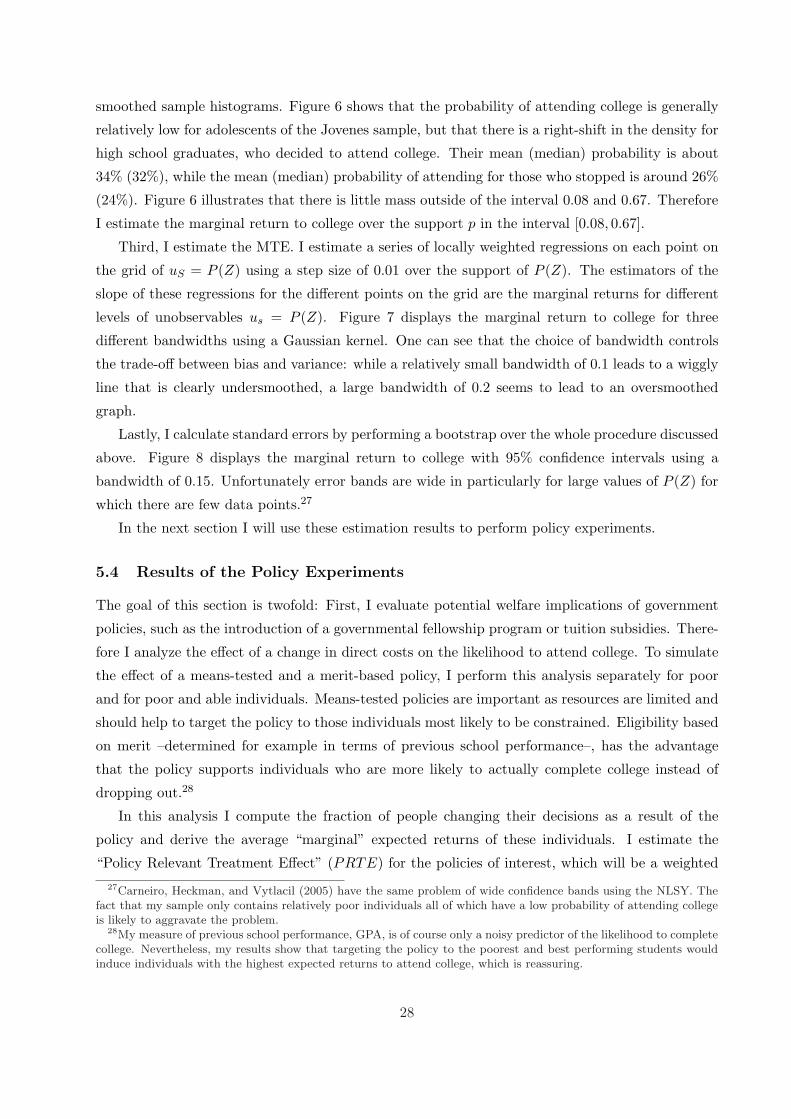
smoothed sample histograms. Figure 6 shows that the probability of attending college is generally

relatively low for adolescents of the Jovenes sample, but that there is a right-shift in the density for

high school graduates, who decided to attend college. Their mean (median) probability is about

34% (32%), while the mean (median) probability of attending for those who stopped is around 26%

(24%). Figure 6 illustrates that there is little mass outside of the interval 0.08 and 0.67. Therefore

I estimate the marginal return to college over the support p in the interval [0.08, 0.67].

Third, I estimate the MTE. I estimate a series of locally weighted regressions on each point on

the grid of uS = P (Z) using a step size of 0.01 over the support of P (Z). The estimators of the

slope of these regressions for the different points on the grid are the marginal returns for different

levels of unobservables us = P (Z). Figure 7 displays the marginal return to college for three

different bandwidths using a Gaussian kernel. One can see that the choice of bandwidth controls

the trade-off between bias and variance: while a relatively small bandwidth of 0.1 leads to a wiggly

line that is clearly undersmoothed, a large bandwidth of 0.2 seems to lead to an oversmoothed

graph.

Lastly, I calculate standard errors by performing a bootstrap over the whole procedure discussed

above. Figure 8 displays the marginal return to college with 95% confidence intervals using a

bandwidth of 0.15. Unfortunately error bands are wide in particularly for large values of P (Z) for

which there are few data points.27

In the next section I will use these estimation results to perform policy experiments.

5.4 Results of the Policy Experiments

The goal of this section is twofold: First, I evaluate potential welfare implications of government

policies, such as the introduction of a governmental fellowship program or tuition subsidies. There-

fore I analyze the effect of a change in direct costs on the likelihood to attend college. To simulate

the effect of a means-tested and a merit-based policy, I perform this analysis separately for poor

and for poor and able individuals. Means-tested policies are important as resources are limited and

should help to target the policy to those individuals most likely to be constrained. Eligibility based

on merit –determined for example in terms of previous school performance–, has the advantage

that the policy supports individuals who are more likely to actually complete college instead of

dropping out.28

In this analysis I compute the fraction of people changing their decisions as a result of the

policy and derive the average “marginal” expected returns of these individuals. I estimate the

“Policy Relevant Treatment Effect” (PRTE) for the policies of interest, which will be a weighted27Carneiro, Heckman, and Vytlacil (2005) have the same problem of wide confidence bands using the NLSY. The

fact that my sample only contains relatively poor individuals all of which have a low probability of attending collegeis likely to aggravate the problem.

28My measure of previous school performance, GPA, is of course only a noisy predictor of the likelihood to completecollege. Nevertheless, my results show that targeting the policy to the poorest and best performing students wouldinduce individuals with the highest expected returns to attend college, which is reassuring.

28

average of the marginal returns to college (MTE), as determined in the previous section. For the

evaluation of policies it is crucial to derive the “marginal” return instead of the “average” return

of a randomly selected individual, because only the people “at the margin” are the ones who will

respond to policies.

Second, I test whether the average “marginal” expected return is significantly larger than the

average expected return of individuals attending college. Thus with subjective expectations I can

improve on the test suggested by Card (2001). Larger “marginal” returns indicate that individuals

at the margin face higher unobserved costs.

The first policy I evaluate is a decrease in the distance to the closest university. This could be

seen as a literal decrease in the distance by building new universities in places that previously did

not have higher education institutions or as a reduction in direct costs via fellowships for costs of

living. Of course the implied costs of the two policies are likely to be very different and are very

difficult to determine. In addition the analysis in this section does not take into account general

equilibrium effects of government policies. Thus the goal of this section is not a complete cost-

benefit-analysis, but to test for credit constraints by comparing expected returns of people at the

margin to the ones of those already attending and to give an idea of potential welfare benefits of

government policies such as fellowship programs in Mexico.

In Section 4.2 I have shown that a change in distance to college affects poor high-return in-

dividuals most. In addition I take into account in this section, that a change in costs can only

affect individuals at the margin. I perform the analysis by decreasing the distance to college by 20

kilometers (for different target groups). This counterfactual policy leads to an increase in college

attendance of about 4% (1 percentage points), and to an average marginal expected return of 0.91

(see Table 7). Decreasing the distance only for very poor individuals (less than 5,000 pesos per

capita income), leads to a change in attendance of 2%, while those individuals who change college

attendance have an average marginal expected return of 0.92. For very poor and very able indi-

viduals (per capita income less than 5,000 pesos and GPA in the top tercile), this policy would

lead to a change in attendance of about 1%, and an average marginal expected return of 0.93. The

expected returns of this last group (very poor and high-performing) is significantly larger that the

average expected return of people already attending (0.71), while one cannot reject that the average

expected return of the other two groups at the margin is as high as the return of those already

attending. These results imply that individuals at the margin have to be facing high unobserved

costs to explain the fact that they did not attend college despite high expected returns.

As a second policy experiment, I consider the effect of a 10% decrease in tuition costs, for

example via tuition subsidies. A 10% reduction in tuition costs leads to an average marginal return

of 0.83, 0.79 for the poor and 0.81 for the poor and able, which is as high as the average expected

return of those individuals attending (see Table 7). Unfortunately, tuition costs are very noisily

measured, so standard errors for the fraction of “switchers” and for the marginal returns are large.

29

Again, for a full cost-and-benefit analysis one would have to take into account the costs of a

government policy. If a large-scale policy is put in place, one would additionally have to take into

account general equilibrium effects, in particular in terms of skill prices. It would be an interesting

topic for future research to analyze how people update beliefs about future returns to schooling

given the introduction of such a policy.

6 Conclusion

The goal of this paper has been to improve our understanding of the huge differences in college

enrollment rates between poor and rich students in Mexico and to show how data on people’s

subjective expectations of earnings can help in this endeavor.

When examining reasons for low school attendance among the poor, researchers face the follow-

ing identification problem: On the one hand poor people might expect particularly low returns to

schooling –due for example to lower cognitive skills or perceptions of limited career opportunities

even with a college degree–, and thus decide not to attend. On the other hand they might face

high attendance costs that prevent them from attending despite high expected returns.

To address this identification problem, I use data on people’s subjective expectations of their

idiosyncratic returns to college as well as on their college attendance choice. Since what matters for

people’s decisions is the perception of their own cognitive and social skills and their beliefs about

future skill prices, these data ideally provide people’s expectations conditional on their information

sets at the time of the decision. These data thus help to relax strong assumptions of conventional

approaches about people’s information sets and about how they form expectations, which were

necessary to address the identification problem in the absence of data on subjective expectations.

My results have shown that poor individuals require significantly higher expected returns to

be induced to attend college, implying that they face higher costs than individuals with wealthy

parents. I found that poor individuals with high expected returns are particularly responsive to

changes in direct costs, which is consistent with the predictions of a model with credit constraints.

Evaluating potential welfare implications by applying the Local Instrumental Variables approach

of Heckman and Vytlacil (2005) to my model, I found that a sizeable fraction of poor individuals

would change their decision and attend in response to a reduction in direct costs. Individuals at

the margin have expected returns that are as high or higher than the ones of individuals already

attending college, which is consistent with credit constraints playing an important role.

My results suggest that credit constraints are one of the driving forces of Mexico’s large in-

equalities in access to higher education and low overall enrollment rates and point to large welfare

gains of introducing a governmental fellowship program by removing obstacles to human capital

accumulation and fostering Mexico’s development and growth.

30

References

Attanasio, O. P., and K. M. Kaufmann (2009): “Educational Choices, Subjective Expectations

and Credit Constraints,” NBER Working Paper 15087, July.

Becker, G. S. (1967): Human Capital: A Theoretical and Empirical Analysis, with Special Ref-

erence to Education. Chicago: University of Chicago Press.

Behrman, J. R., A. Gaviria, and M. Szekely (2002): Social Exclusion in Latin America:

Introduction and Overview. Social Exclusion in Latin America and the Caribbean. Washington,

D.C.: Inter-American Development Bank.

Belzil, C., and J. Hansen (2002): “Earnings Dispersion, Risk Aversion, and Education,” IZA

Discussion Paper No. 513.

Binelli, C. (2008): “Returns to Education and Increasing Wage Inequality in Latin America,”

mimeo.

Blossfeldt, H., and Y. Shavit (1993): Persistent Inequality: Changing Educational Attainment

in Thirteen Countries. Boulder, Co: Westview Press.

Cameron, S. V., and J. J. Heckman (1998): “Life Cycle Schooling and Dynamic Selection Bias:

Models and Evidence for Five Cohorts of American Males,” Journal of Political Economy, 106

(2), 262–333.

(2001): “The Dynamics of Educational Attainment for Black, Hispanic and White Males,”

Journal of Political Economy, 109 (3), 455–499.

Cameron, S. V., and C. Taber (2004): “Borrowing Constraints and the Returns to Schooling,”

Journal of Political Economy, 112 (1), 132–182.

Card, D. (1995): Using Geographic Variation in College Proximity to Estimate the Return to

Schooling, In: Aspects of Labour Market Behaviour: Essays in Honour of John Vanderkamp.

Toronto: Univ. Toronto Press.

(2001): “Estimating the Return to Schooling: Progress on Some Persistent Econometric

Problems,” Econometrica, 69 (5), 1127–60.

Carneiro, P., and J. J. Heckman (2002): “The Evidence on Credit Constraints in Post-

Secondary Schooling,” The Economic Journal, 112 (October), 705–734.

Carneiro, P., J. J. Heckman, and E. Vytlacil (2005): “Understanding What IV Estimate:

Estimating Marginal and Average Returns to Education,” mimeo.

31

Connolly, H., and P. Gottschalk (2006): “Differences in Wage Growth by Education Level -

Do Less-Educated Workers Gain Less from Work Experience?,” mimeo.

Cunha, F., and J. J. Heckman (2006): “A New Framework for the Analysis of Inequality,”

NBER working paper 12505.

Cunha, F., J. J. Heckman, and S. Navarro (2005): “Separating Uncertainty from Heterogene-

ity in Life Cycle Earnings,” Oxford Economic Papers, 57, 191–261.

Delavande, A., X. Gine, and D. McKenzie (2009): “Measuring Subjective Expectations in

Developing Countries: A Critical Review and New Evidence,” World Bank Policy Research

Working Paper No. 4824.

Dominitz, J., and C. F. Manski (1996): “Eliciting Student Expectations of the Returns to

Schooling,” Journal of Human Resources, 31 (1), 1–26.

Fan, J. (1992): “Design-Adaptive Nonparametric Regression,” Journal of the American Statistical

Association, 87, 998–1004.

Guiso, L., T. Jappelli, and L. Pistaferri (2002): “An Empirical Analysis of Earnings and

Employment Risk,” Journal of Business and Economic Statistics, 20 (2), 241–253.

Heckman, J. J., L. Lochner, and C. Taber (1998): “Explaining Rising Wage Inequality:

Explorations with a Dynamic General Equilibrium Model of Labor Earnings with Heterogeneous

Agents,” Review of Economic Dynamics, 1, 1–58.

Heckman, J. J., and E. Vytlacil (2001): “Policy-Relevant Treatment Effects,” American Eco-

nomic Review, Papers and Proceedings, 91 (2), 107–111.

(2005): “Structural Equations, Treatment Effects, and Econometric Policy Evaluation,”

Econometrica, 73 (3), 669–738.

Heckman, J. J., E. Vytlacil, and S. S. Urzua (2006): “Understanding Instrumental Variables

in Models with Essential Heterogeneity,” mimeo.

Jensen, R. (forthcoming): “The (Perceived) Returns to Education and the Demand for Schooling,”

Quarterly Journal of Economics.

Kaufmann, K. M. (2008): “Understanding the Income Gradient in College Attendance in Mexico:

The Role of Heterogeneity in Expected Returns to College,” SIEPR Working Paper, January

2008, 07-040.

Kaufmann, K. M., and L. Pistaferri (2009): “Disentangling Insurance and Information in In-

tertemporal Consumption Choices,” American Economic Review, Papers and Proceedings, 99(2),

387–92.

32

Kling, J. R. (2001): “Interpreting Instrumental Variables Estimates of the Returns to Schooling,”

Journal of Business and Economic Statistics, 19 (July), 358–364.

Manski, C. F. (2004): “Measuring Expectations,” Econometrica, 72 (5), 1329–76.

McKenzie, D. (2006): “The Consumer Response to the Mexican Peso Crisis,” Economic Devel-

opment and Cultural Change, 55(1), 139–172.

Mincer, J. (1974): “Schooling, Experience and Earnings,” NBER, New York.

Nguyen, T. (2008): “Information, Role Models and Perceived Returns to Education: Experimen-

tal Evidence from Madagascar,” mimeo.

Padula, M., and L. Pistaferri (2001): “Education, Employment and Wage Risk,” Working

Paper No. 67, Centre for the Studies in Economics and Finance.

Stinebrickner, R., and T. R. Stinebrickner (2008): “The Effect of Credit Constraints on

the College Drop-Out Decision: A Direct Approach Using a New Panel Study,” The American

Economic Review, 98(5), 2163–84.

(2009): “Learning about Academic Ability and the College Drop-Out Decision,” mimeo.

Willis, R. J., and S. Rosen (1979): “Education and Self-Selection,” Journal of Political Econ-

omy, 87, S 7–36.

33

Appendix A

Figure 1: Comparing Expectations of High School Graduates with a One-Year Younger Cohort

0.2

.4.6

.81

Ker

nel d

ensi

ty

6 6.5 7 7.5 8 8.5 9 9.5 10Expected College Earnings

Students in Grade 12 High School Graduates

Expected College Earnings

Figure 2: Comparing Expectations of High School Graduates with a One-Year Younger Cohort

0.2

.4.6

.81

Ker

nel d

ensi

ty

6 6.5 7 7.5 8 8.5 9 9.5 10Expected High School Earnings

Students in Grade 12 High School Graduates

Expected High School Earnings

34

Figure 3: The Triangular Distribution of Earnings

p1-p

min maxmidmode x

f(x)

Figure 4: The Cumulative Distribution Function of Costs for Different Income Classes.

.2.2

5.3

.35

.4.4

5.5

Cdf

of C

osts

.2 .4 .6 .8 1 1.2College Attendance Costs

High Income Middle Income Low Income

Cumulative distribution function of Costs by Income Class

35

Figure 5: The Cumulative Distribution Function of Costs with 95% Confidence Intervals.

.2.2

5.3

.35

.4.4

5.5

Cdf

of C

osts

.2 .4 .6 .8 1 1.2College Attendance Costs

High Income: Cdf of Costs with 95% CILow Income: Cdf of Costs with 95% CI

Cumulative distribution function of Costs by Income Class

Figure 6: The Predicted Probability of Attending College.

01

23

4D

ensi

ty o

f P

0 .1 .2 .3 .4 .5 .6 .7 .8 .9 1P

HS Grad Not Enrolled in CollegeHS Grad Enrolled in College

Predicted Probability of College Attendance

36

Figure 7: The Marginal Return to College for Different Levels of Unobserved Costs.

.82

.84

.86

.88

.9.9

2

0 .1 .2 .3 .4 .5 .6 .7 .8 .9 1u

MTE(u), BW=0.1MTE(u), BW=0.15MTE(u), BW=0.2

MT

E(u

)

Marginal Return: MTE(u))

Figure 8: The Marginal Return to College with 95% Confidence Interval Bands.

.4.6

.81

1.2

1.4

0 .1 .2 .3 .4 .5 .6 .7 .8 .9 1u

Upper Bound of 95% CIMarginal Return: MTE(u) (BW=0.15)Lower Bound of 95% CI

MT

E(u

)

Marginal Return with Confidence Intervals

37

Table 1: Summary Statistics.

Variable Obs Mean Std. Dev. Median

Expected Return 1612 0.6670 0.3820 0.6047Expected Log High School Earnings 1612 7.5778 0.5004 7.6432Var of Log High School Earnings 1612 0.0054 0.0079 0.0028Var of Log College Earnings 1612 0.0039 0.0061 0.0019Prob of Work High School 1612 0.6657 0.1817 0.7Prob of Work College 1612 0.8250 0.1601 0.9

College Attendance Rate 1612 0.2308 0.4215 0

Female 1612 0.5813 0.4935 1

GPA (Scale 0 to 100) 1612 82.19 7.16 82GPA Second Tercile 1612 0.2804 0.4493 0GPA Top Tercile 1612 0.2773 0.4478 0

Father’s Yrs of Schooling 951 5.33 2.96 6Father’s Educ Jr High School 1612 0.1067 0.3088 0

Sr High School 1612 0.0292 0.1683 0College 1612 0.0050 0.0703 0

Mother’s Yrs of Schooling 1140 5.03 2.77 5Mother’s Educ Jr High School 1612 0.1234 0.3291 0

Sr High School 1612 0.0174 0.1307 0College 1612 0.0037 0.0609 0

Per Capital Parental Income (Pesos) 1187 7519.54 8010.08 5200Per Capita Parental Income < 5000 Pesos 1612 0.5906 0.4692 1

5000 to 10000 Pesos 1612 0.2407 0.4276 0> 10000 Pesos 1612 0.1687 0.3746 0

Distance to University (km) 1612 24.2312 22.8159 18.26Distance to University < 20 km 1612 0.5298 0.4993 1

20 to 40 km 1612 0.2599 0.4387 0> 40 km 1612 0.2103 0.4076 0

Tuition Costs (Pesos) 1171 608.8104 634.5729 750Tuition Costs above 750 Pesos 1612 0.4187 0.4935 0

38

Table 2: Probit Model of the College Attendance Decision.

Dep. Var.: Attend College Model 1 Model 2 Model 3Marg. Eff./(S.E.) Marg. Eff./(S.E.) Marg. Eff./(S.E.)

Expected Return to College 0.092*** 0.078** 0.077**(0.033) (0.034) (0.034)

Prob of Work - Sr HS 0.032 0.013 0.005(0.087) (0.085) (0.081)

Prob of Work - College -0.008 -0.001 0.032(0.101) (0.099) (0.092)

Var of Log Earn - Sr HS -2.625 -3.016 -2.959(1.919) (2.008) (1.958)

Var of Log Earn - College -0.310 0.036 0.196(2.351) (2.291) (2.164)

Female -0.055* -0.059* -0.046(0.029) (0.033) (0.032)

GPA - Second Tercile 0.055* 0.055*(0.031) (0.031)

GPA - Top Tercile 0.187*** 0.174***(0.038) (0.045)

Father’s Educ - Jr HS 0.099** 0.073*(0.042) (0.042)

Father’s Educ - Sr HS 0.151* 0.100(0.078) (0.075)

Father’s Educ - Univ 0.547*** 0.574***(0.120) (0.131)

Mother’s Educ - Jr HS 0.100** 0.074*(0.040) (0.039)

Mother’s Educ - Sr HS 0.203** 0.173*(0.099) (0.101)

Per Cap Income - 5 to 10k 0.051*(0.031)

Per Cap Income - more than 10k 0.119***(0.037)

Dist to Univ 20 to 40km -0.076***(0.029)

Dist to Univ above 40km -0.106***(0.031)

Tuition Above 750 Pesos -0.082**(0.039)

State FE Yes Yes Yes

Observations (Censored) 3342 (1730) 3342 (1730) 3342 (1730)Log Likelihood -3041.971 -2990.349 -2972.964Sample Sel.: Corr. betw. Errors (P-Val) -0.487 (0.055) -0.282 (0.314) -0.131 (0.654)

Notes: Table displays marginal effects and standard errors in brackets. * p<0.1 ** p<0.05 *** p<0.01. Excl. categories: male, lowest GPA tercile,father’s and mother’s education primary or less (mother’s education university not displayed, as not significant due to small number of obs), percapita income less than 5000 pesos, distance to university less than 20 km and tuition less than 750 pesos.

39

Table 3: Excess Responsiveness of the Poor to Changes in Direct Costs (Distance to College).

Dep. Var.: Attend College Model 4 Model 5 Model 6Marg. Eff./(S.E.) Marg. Eff./(S.E.) Marg. Eff./(S.E.)

Univ 20 - 40km * Par Income < 5k -0.089** -0.092** -0.076(0.044) (0.044) (0.059)

Univ 20 - 40km * Par Income < 5k * High Exp Ret -0.067(0.083)

Univ 20 - 40km * Par Income 5 - 10k -0.044 -0.049 -0.041(0.054) (0.054) (0.078)

Univ 20 - 40km * Par Income 5 - 10k * High Exp Ret -0.022(0.109)

Univ 20 - 40km * Par Income > 10k 0.053 0.048 0.062(0.071) (0.070) (0.099)

Univ 20 - 40km * Par Income > 10k * High Exp Ret -0.026(0.119)

Univ > 40km * Par Income < 5k -0.048 -0.051 -0.041(0.043) (0.043) (0.058)

Univ > 40km * Par Income < 5k * High Exp Ret -0.064(0.081)

Univ > 40km * Par Income 5 - 10k -0.136*** -0.145*** -0.160**(0.051) (0.050) (0.069)

Univ > 40km * Par Income 5 - 10k * High Exp Ret 0.046(0.152)

Univ > 40km * Par Income > 10k -0.045 -0.047 -0.152**(0.071) (0.072) (0.075)

Univ > 40km * Par Income > 10k * High Exp Ret 0.292(0.200)

Par Income < 5k * High Exp Ret 0.088(0.059)

Par Income 5 - 10k * High Exp Ret 0.184**(0.084)

Par Income > 10k * High Exp Ret 0.132(0.093)

Controls for Expected Return, Exp Log Earn,Prob of Work and Var of Log Earn No Yes YesControls: GPA, Par Income and Educ, Sex, State FE Yes Yes Yes

Observations (Censored) 3342 (1730) 3342 (1730) 3342 (1730)Log Likelihood -2984.591 -2971.787 -2965.898Sample Sel.: Corr. betw. Errors (P-Val) -0.167 (0.569) -0.172 (0.556) -0.112 (0.709)

Notes: Table displays marginal effects and standard errors in brackets. * p<0.1, ** p<0.05, *** p<0.01. Excl. categories: male, lowest GPAtercile, parents’ education primary or less, per capita income less than 5000 pesos, interactions of distance to university of less than 20km withparental income and low expected return interacted with parental (per capita) income.

40

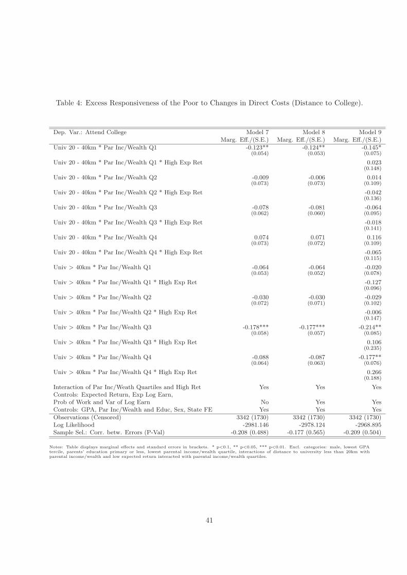
Table 4: Excess Responsiveness of the Poor to Changes in Direct Costs (Distance to College).

Dep. Var.: Attend College Model 7 Model 8 Model 9Marg. Eff./(S.E.) Marg. Eff./(S.E.) Marg. Eff./(S.E.)

Univ 20 - 40km * Par Inc/Wealth Q1 -0.123** -0.124** -0.145*(0.054) (0.053) (0.075)

Univ 20 - 40km * Par Inc/Wealth Q1 * High Exp Ret 0.023(0.148)

Univ 20 - 40km * Par Inc/Wealth Q2 -0.009 -0.006 0.014(0.073) (0.073) (0.109)

Univ 20 - 40km * Par Inc/Wealth Q2 * High Exp Ret -0.042(0.136)

Univ 20 - 40km * Par Inc/Wealth Q3 -0.078 -0.081 -0.064(0.062) (0.060) (0.095)

Univ 20 - 40km * Par Inc/Wealth Q3 * High Exp Ret -0.018(0.141)

Univ 20 - 40km * Par Inc/Wealth Q4 0.074 0.071 0.116(0.073) (0.072) (0.109)

Univ 20 - 40km * Par Inc/Wealth Q4 * High Exp Ret -0.065(0.115)

Univ > 40km * Par Inc/Wealth Q1 -0.064 -0.064 -0.020(0.053) (0.052) (0.078)

Univ > 40km * Par Inc/Wealth Q1 * High Exp Ret -0.127(0.096)

Univ > 40km * Par Inc/Wealth Q2 -0.030 -0.030 -0.029(0.072) (0.071) (0.102)

Univ > 40km * Par Inc/Wealth Q2 * High Exp Ret -0.006(0.147)

Univ > 40km * Par Inc/Wealth Q3 -0.178*** -0.177*** -0.214**(0.058) (0.057) (0.085)

Univ > 40km * Par Inc/Wealth Q3 * High Exp Ret 0.106(0.235)

Univ > 40km * Par Inc/Wealth Q4 -0.088 -0.087 -0.177**(0.064) (0.063) (0.076)

Univ > 40km * Par Inc/Wealth Q4 * High Exp Ret 0.266(0.188)

Interaction of Par Inc/Weath Quartiles and High Ret Yes Yes YesControls: Expected Return, Exp Log Earn,Prob of Work and Var of Log Earn No Yes YesControls: GPA, Par Inc/Wealth and Educ, Sex, State FE Yes Yes Yes

Observations (Censored) 3342 (1730) 3342 (1730) 3342 (1730)Log Likelihood -2981.146 -2978.124 -2968.895Sample Sel.: Corr. betw. Errors (P-Val) -0.208 (0.488) -0.177 (0.565) -0.209 (0.504)

Notes: Table displays marginal effects and standard errors in brackets. * p<0.1, ** p<0.05, *** p<0.01. Excl. categories: male, lowest GPAtercile, parents’ education primary or less, lowest parental income/wealth quartile, interactions of distance to university less than 20km withparental income/wealth and low expected return interacted with parental income/wealth quartiles.

41

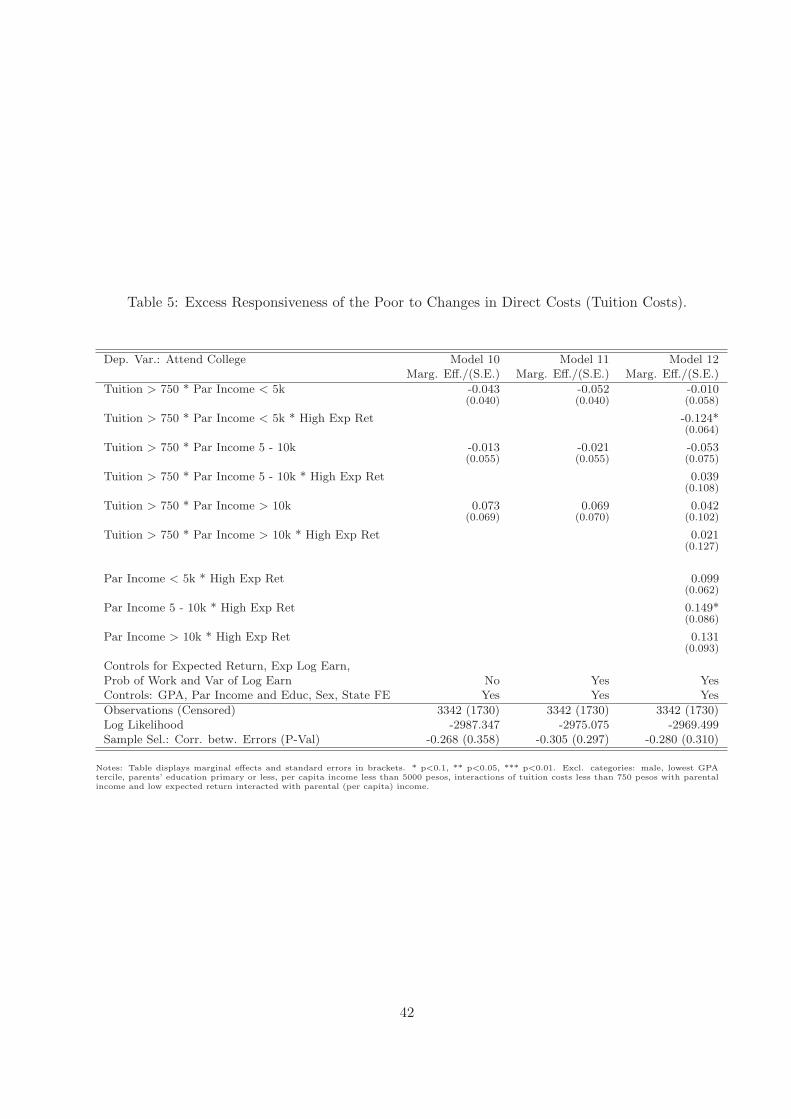
Table 5: Excess Responsiveness of the Poor to Changes in Direct Costs (Tuition Costs).

Dep. Var.: Attend College Model 10 Model 11 Model 12Marg. Eff./(S.E.) Marg. Eff./(S.E.) Marg. Eff./(S.E.)

Tuition > 750 * Par Income < 5k -0.043 -0.052 -0.010(0.040) (0.040) (0.058)

Tuition > 750 * Par Income < 5k * High Exp Ret -0.124*(0.064)

Tuition > 750 * Par Income 5 - 10k -0.013 -0.021 -0.053(0.055) (0.055) (0.075)

Tuition > 750 * Par Income 5 - 10k * High Exp Ret 0.039(0.108)

Tuition > 750 * Par Income > 10k 0.073 0.069 0.042(0.069) (0.070) (0.102)

Tuition > 750 * Par Income > 10k * High Exp Ret 0.021(0.127)

Par Income < 5k * High Exp Ret 0.099(0.062)

Par Income 5 - 10k * High Exp Ret 0.149*(0.086)

Par Income > 10k * High Exp Ret 0.131(0.093)

Controls for Expected Return, Exp Log Earn,Prob of Work and Var of Log Earn No Yes YesControls: GPA, Par Income and Educ, Sex, State FE Yes Yes Yes

Observations (Censored) 3342 (1730) 3342 (1730) 3342 (1730)Log Likelihood -2987.347 -2975.075 -2969.499Sample Sel.: Corr. betw. Errors (P-Val) -0.268 (0.358) -0.305 (0.297) -0.280 (0.310)

Notes: Table displays marginal effects and standard errors in brackets. * p<0.1, ** p<0.05, *** p<0.01. Excl. categories: male, lowest GPAtercile, parents’ education primary or less, per capita income less than 5000 pesos, interactions of tuition costs less than 750 pesos with parentalincome and low expected return interacted with parental (per capita) income.

42

Table 6: Excess Responsiveness of the Poor to Changes in Direct Costs (Tuition Costs).

Dep. Var.: Attend College Model 13 Model 14 Model 15Marg. Eff./(S.E.) Marg. Eff./(S.E.) Marg. Eff./(S.E.)

Tuition > 750 * Par Inc/Wealth Q1 -0.064 -0.067 -0.000(0.048) (0.047) (0.071)

Tuition > 750 * Par Inc/Wealth Q1 * High Exp Ret -0.148*(0.084)

Tuition > 750 * Par Inc/Wealth Q2 -0.037 -0.037 -0.006(0.065) (0.064) (0.095)

Tuition > 750 * Par Inc/Wealth Q2 * High Exp Ret -0.055(0.118)

Tuition > 750 * Par Inc/Wealth Q3 -0.051 -0.055 -0.087(0.062) (0.061) (0.094)

Tuition > 750 * Par Inc/Wealth Q3 * High Exp Ret 0.038(0.137)

Tuition > 750 * Par Inc/Wealth Q4 0.069 0.066 0.117(0.070) (0.070) (0.104)

Tuition > 750 * Par Inc/Wealth Q4 * High Exp Ret -0.106(0.101)

Interaction of Par Inc/Weath Quartiles and High Ret Yes Yes YesControls: Expected Return, Exp Log Earn,Prob of Work and Var of Log Earn No Yes YesControls: GPA, Par Inc/Wealth and Educ, Sex, State FE Yes Yes Yes

Observations (Censored) 3342 (1730) 3342 (1730) 3342 (1730)Log Likelihood -2987.524 -2984.668 -2972.787Sample Sel.: Corr. betw. Errors (P-Val) -0.329 (0.236) -0.309 (0.275) -0.326 (0.247)

Notes: Table displays marginal effects and standard errors in brackets. * p<0.1, ** p<0.05, *** p<0.01. Excl. categories: male, lowest GPAtercile, parents’ education primary or less, lowest parental income/wealth quartile, interactions of tuition costs less than 750 pesos with parentalincome/wealth and low expected return interacted with parental income/wealth quartiles.

43

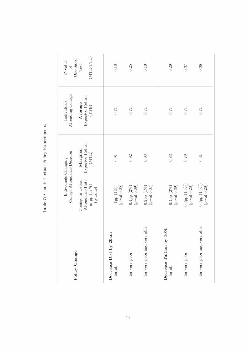
Tab

le7:

Cou

nter

fact

ualPol

icy

Exp

erim

ents

.

Indi

vidu

als

Cha

ngin

gIn

divi

dual

sP

-Val

ueC

olle

geA

tten

danc

eD

ecis

ion

Att

endi

ngC

olle

geof

Pol

icy

Chan

geO

ne-S

ided

Cha

nge

inO

vera

llM

argi

nal

Ave

rage

Tes

tA

tten

danc

eR

ate

Exp

ecte

dR

etur

nE

xpec

ted

Ret

urn

inpp

(in

%)

(MT

E)

(TT

E)

(MT

E-T

TE

)(p

-val

ue)

Dec

reas

eD

ist

by

20km

for

all

1pp

(4%

)0.

910.

710.

18(p

-val

0.05

)

for

very

poor

0.4p

p(2

%)

0.92

0.71

0.25

(p-v

al0.

09)

for

very

poor

and

very

able

0.2p

p(1

%)

0.93

0.71

0.10

(p-v

al0.

07)

Dec

reas

eTuit

ion

by

10%

for

all

0.4p

p(2

%)

0.83

0.71

0.29

(p-v

al0.

39)

for

very

poor

0.3p

p(1

.5%

)0.

790.

710.

37(p

-val

0.28

)

for

very

poor

and

very

able

0.3p

p(1

.5%

)0.

810.

710.

36(p

-val

0.28

)

44

Appendix B

Derivation of the Participation Equation

In order to use the potential outcome equations (2) and the subjective expectation information (3),

and rewrite the participation equation in terms of expected returns to college, I use the following

approximation

E(Yia) ≡ E(eln Yia) ∼= eE(ln Yia)+0.5V ar(ln Yia) (15)

and assume that V ar(lnY Sia) = (σS

i )2 for all a and S = 0, 1.

Thus I can rewrite the expected present value of college earnings (analogously for high school

earnings) as

EPV18(Y 1i ) =

∞∑

a=22

pW1i exp(E18(lnY 1

ia) + 0.5V ar18(lnY 1ia))

(1 + ri)a−18

=∞∑

a=22

pW1i exp

(α1 + β′1Xi + γ1p

W1i (a− 22) + θ′1fi + 0.5(σ1

i )2)

(1 + ri)a−18

=pW1

i exp(α1 + β′1Xi + θ′1fi + 0.5(σ1

i )2)

(1 + ri)4·( ∞∑

a=22

exp(γ1p

W1i (a− 22)

)

(1 + ri)a−22

)

=pW1

i exp(α1 + β′1Xi + θ′1fi + 0.5(σ1

i )2)

(1 + ri)4

(1 + ri

1 + ri − exp(γ1pW1i )

), (16)

where I assume that exp(γjpWji ) < 1 + ri for j = 0, 1 to apply the rule for a geometric series,29

and I use A →∞ as an approximation.

Data on subjective expectations of earnings for age a = 25 allow me to rewrite the expected

present value of college earnings as follows (see equation (3)):

EPV18(Y 1i ) =

pW1i exp

(E18(lnY 1

i25) + 0.5(σ1i )

2 − 3γ1pW1i

)

(1 + ri)3·(

11 + ri − exp(γ1pW1

i )

),

Analogously, I can derive the following expression for EPV18(Y 0i )

EPV18(Y 0i ) = pW0

i exp(α0 + β′0Xi + θ′0fi + 0.5(σ0

i )2) ·

(1 + ri

1 + ri − exp(γ0pW0i )

). (17)

An individual decides to attend college if EPV18(Y 1i )−EPV18(Y 0

i )− Ci

pCi≥ 0, and thus if

29Some back-of-the-envelope calculations suggest that this assumption is reasonable in the given context: Paperssuch as Connolly and Gottschalk (2006) and Heckman, Lochner, and Taber (1998) find returns to experience wellbelow 0.05 for the US, while interest rates in Mexico are clearly significantly higher than 0.05 in the relevant period(see for example McKenzie (2006)).

45

[pW1

i exp(E18(lnY 1

i25) + 0.5(σ1i )

2 − 3γ1pW1i

)

(1 + ri)3·(

11 + ri − exp(γ1pW1

i )

)]

−[pW0

i exp(E18(lnY 0

i25) + 0.5(σ0i )

2 − 7γ0pW0i

) ·(

1 + ri

1 + ri − exp(γ0pW0i )

)]− Ci

pCi

≥ 0,

which I can rewrite in the following way

exp(E18(lnY 1

i25) + 0.5(σ1i )

2)− exp

(E18(lnY 0

i25) + 0.5(σ0i )

2)

·[(1 + ri)4

pW0i

pW1i

· exp(3γ1pW1i )

exp(7γ0pW0i )

(1 + ri − exp(γ1p

W1i )

1 + ri − exp(γ0pW0i )

)]

≥ (1 + ri)3Ci

pCi pW1

i

(1 + ri − exp(γ1pW1i ))

Assumption:(

1+ri−exp(γ1pW1i )

1+ri−exp(γ0pW0i )

)≈ 1, which is approximately satisfied given estimates of returns

to experience of around 0.03 for college and 0.02 for high school and an interest rate of around

10% (see, for example, as mentioned above Connolly and Gottschalk (2006) using SIPP data for

the US or Heckman, Lochner, and Taber (1998) who show that differences in returns to experience

between high school and college educated are small).

In order to express the decision rule (18) in terms of expected gross returns to college and use

the information on expected returns from ‘subjective’ expectations of earnings (see expression (4)),

I use a Taylor series approximation of exp(B) around A, exp(B) = exp(A)∑∞

j=0(B−A)j

j! , to rewrite

the decision rule, which has the form exp(B)− exp(A) · L ≥ K. Noting that in this context

B −A =(E18(lnY 1

i25) + 0.5(σ1i )

2)− (

E18(lnY 0i25) + 0.5(σ0

i )2)

= ρi25 + 0.5((σ1

i )2 − (σ0

i )2),

I can write the decision rule as

exp(E18(lnY 0

i25) + 0.5(σ0i )

2) ·

∞∑

j=0

(ρi25 + 0.5

((σ1

i )2 − (σ0

i )2))j

j!

− (exp(E18(lnY 0

i25) + 0.5(σ0i )

2)) · (1 + ri)4

pW0i

pW1i

· exp(3γ1pW1i )

exp(7γ0pW0i )

− (1 + ri)3Ci

pCi pW1

i

(1 + ri − exp(γ1)) ≥ 0.

Rearranging will lead to

∞∑

j=0

(ρi25 + 0.5

((σ1

i )2 − (σ0

i )2))j

j!

− (1 + ri)4

[pW0

i

pW1i

· exp(3γ1pW1i )

exp(7γ0pW0i )

+Ci

pCi pW1

i exp(E(lnY 0

i25) + 0.5(σ0i )2

)]

+(1 + ri)3Ci

pCi pW1

i exp(E(lnY 0

i25) + 0.5(σ0i )2

) exp(γ1pW1i ) ≥ 0.

46

Thus using the ‘subjective’ expectation information, the latent variable model for attending

university can be written as

S∗ =

∞∑

j=0

(ρi25 + 0.5

((σ1

i )2 − (σ0

i )2))j

j!

−(1 + ri)4[

pW0i

pW1i

· exp(3γ1pW1i )

exp(7γ0pW0i )

+Ci

pCi pW1

i exp(E(lnY 0

i25) + 0.5(σ0i )2

)]

(18)

+(1 + ri)3Ci

pCi pW1

i exp(E(lnY 0

i25) + 0.5(σ0i )2

) exp(γ1pW1i ) ≥ 0.

S = 1 if S∗ ≥ 0

S = 0 otherwise,

where S is a binary variable indicating the treatment status.

Derivation of the Testable Prediction of Excess Responsiveness

Making use of the participation equation for college attendance (see equation (18)), the following

results show that individuals who face a higher interest rate are more responsive to changes in

direct costs.

∂S∗

∂C=−(1 + ri)4 + (1 + ri)3 exp(γ1p

W1i )

pCi pW1

i exp(E(lnY 0

i25) + 0.5(σ0i )2

) < 0

as exp(γ1pW1i ) < 1 + ri (see the previous section). Furthermore

∂2S∗

∂C∂r=−4(1 + ri)3 + 3(1 + ri)2 exp(γ1p

W1i )

pCi pW1

i exp(E(lnY 0

i25) + 0.5(σ0i )2

) < 0, (19)

as 4(1 + ri) > 3 exp(γ1pW1i ).

Thus∣∣∂S∗

∂C

∣∣ is increasing in ri, that is individuals who face a higher interest rate are more

responsive to changes in direct costs.

Participation Equation as a Fourth-Order Polynomial in the Interest Rate

The participation equation (18) can be expressed as polynomial in the interest rate (so that r is

left as the unobservable)

(1 + r)4 − (1 + r)3C exp(γ1)(

pCi pW1

i exp(E(lnY 0

i25) + 0.5(σ0i )2

)) · pW0i

pW1i

· exp(γ13)exp(γ07) + C

−

∞∑

j=0

(ρi + 0.5

((σ1

i )2 − (σ0

i )2))j

j!

pC

i pW1i exp

(E(lnY 0

i25) + 0.5(σ0i )

2)

(pC

i pW1i exp

(E(lnY 0

i25) + 0.5(σ0i )2

)) · pW0i

pW1i

· exp(γ13)exp(γ07) + C

≤ 0.

47

Derivation of the Marginal Return to College

Derivation of equation (12):

E(U1 − U0|US ≤ p) =∫ ∞

−∞(U1 − U0) f(U1 − U0|US ≤ p)d(u1 − u0)

=∫ ∞

−∞(U1 − U0)

∫ p0 f (U1 − U0, US) duS

Pr(US ≤ p)d(u1 − u0)

=∫ ∞

−∞(U1 − U0)

∫ p0 f (U1 − U0|US) f(uS)duS

pd(u1 − u0)

=1p

∫ p

0E (U1 − U0|US = uS) duS .

48

Appendix C

Background Information on College Enrollment and on Costs and Financing of

College Attendance in Mexico

In 2004 around 22% of adolescents of the relevant age group (18 to 24 years) were attending

college in Mexico to receive an undergraduate degree (“licenciatura”) (ANUIES, annual statistics

2004). This attendance rate is significantly lower than in many other Latin American countries (see

Table 8). Mexico is characterized by large inequalities in access to college education for different

income groups. In comparison to other Latin American countries, such as Colombia, Argentina

and Chile, only Brazil has a smaller fraction of poor students attending college (see Table 8).

Figure 9 displays college attendance rates of 18 to 24 year old high school graduates for different

parental income quartiles.30 High school graduates are already a selective group, for example for

urban Mexico about 75% of the relevant age group attain a high school degree. The attendance

rate of high school graduates in the lowest parental income quartile is around 22% compared to

67% for the highest parental income quartile. The “Jovenes con Oportunidades” sample (2005)

used in this paper consists of high school graduates from Oportunidades families and is thus only

representative of about the poorest third of the high school graduate population. The positive

correlation between parental income and college attendance rate can also be found for this sample,

but differences between poorest quartile (17%) and richest quartile (35%) are smaller, as every

individual in the sample is relatively poor (see figure 10, Jovenes con Oportunidades 2005).

College attendance costs in Mexico pocket a large fraction of parental income for relatively

poor families. Costs consist of enrollment and tuition fees, fees for (entrance) exams and other

bureaucratic costs, costs for transport and/or room and board, health insurance (mandatory for

some universities), costs for schooling materials such as books. Administrative data on tuition

and enrollment fees per year from the National Association of Universities and Institutes of Higher

Education (ANUIES) reveals a large degree of heterogeneity: Yearly tuition and enrollment costs

vary between 50 pesos (“Universidad Autonoma de Guerrero”, Guerrero) and 120,000 pesos (“Tec-

nologico de Monterrey”, I.T.E.S.M. - Campus Puebla), which is equivalent to approximately 5

and 12,000 US$. The tuition cost measure that I use in my analysis is the minimum yearly tu-

ition/enrollment fee of universities in the closest locality with at least one university (see section

3.4). Fifty percent of the high school graduates face (minimum) tuition costs of over 750 pesos,

which is equivalent to about 15% of median yearly per capita parental income. The other important

cost factor depends on whether the adolescent has to move to a different city and pay room and

board or whether she can live with her family during college. I therefore construct a measure of

distance to the closest university for each individual (see section 3.4).

In Mexico funding for higher-education fellowships and student loan programs is very limited30Parental income is measured in the last year before the college attendance decision.

49

and only about 5% of the undergraduate student population receive fellowships, while 2% receive

student loans, which is low even compared to other Latin American countries (see Table 8). The

national scholarship program PRONABES was created in 2001 with the goal of more equal access

to higher education at the undergraduate level. In 2005 funding of PRONABES amounted to

850 million pesos (equal to 40 US$ per student per year) and 5% of the undergraduate student

population received a fellowship (“beca”) in 2005 compared to 2% in 2001/02 (see Department of

Public Education (SEP)), 2005). Eligibility for a fellowship is subject to three conditions: first, a

maximum level of family income, where priority is given to families with less than two times the

minimum monthly salary, while in special cases people are still eligible with less than four times

the minimum monthly salary. Second, students need a minimum GPA (80) and third, they have to

have been accepted at a public university or technical institute. After each year, the student has

to prove that economic eligibility criteria are still met and that she is in good academic standing.

In 2004/05 the fellowship consisted of a monthly stipend of 750 pesos –slightly more than half the

minimum wage per month– in the first year of studies, and increased to 1000 pesos in the fourth

year of studies. Student loan programs are also of minor importance in Mexico. Only about 2%

of the national student population benefit from a student loan, which is low even compared to

poorer Latin American countries, such as Colombia (9%) and Brazil (6%). In Mexico there are

four different programs that offer student loans. The largest program, SOFES, offers loans to 1.5%

of students and was implemented by a collaboration of private universities. It is need-and-merit

based, but students with collateral are preferred. The other three are very small state programs,

ICEES in Sonora state, ICEET in Tamaulipas, and Educafin in Guanajuato, which are not part of

my sample.

Figure 9: College enrollment rates of 18 to 24 year old high school completers by parental incomequartile (Mexican Family Life Survey, 2003).

0

10

20

30

40

50

60

70

80

Col

lege

Atte

ndan

ce R

ate

(in %

)

1 2 3 4Parental Income Quartile

Source: Author’s calculation using the Mexican Family Life Survey, 2003.

College Attendance Rates by Parental Income Quartile (MxFLS)

50

Figure 10: College enrollment rates of 18 to 24 year old high school completers by parental incomequartile (Jovenes con Oportunidades Survey, 2005).

0

5

10

15

20

25

30

35

Col

lege

Atte

ndan

ce R

ate

(in %

)

1 2 3 4Parental Income Quartile

Source: Author’s calculation using the Jovenes con Oportunidades Survey, 2005.

College Attendance Rates by Parental Income Quartile (Jov)

51

Tab

le8:

Com

pari

son

ofen

rollm

ent

rate

s,fr

acti

onof

poor

est

40%

inpe

rcen

tof

the

stud

ent

popu

lati

on,fr

acti

onof

GD

Psp

end

onhi

gher

educ

atio

n,fr

acti

onof

expe

ndit

ures

onhi

gher

educ

atio

non

fello

wsh

ips

and

stud

ent

loan

s:M

exic

o,ot

her

Lat

inA

mer

ican

coun

trie

s,O

EC

Dan

dU

SA.

Countr

ies

Enro

llm

ent

inFra

ctio

nofPoore

st40%

Expen

dit

ure

son

Spen

din

gon

Ben

efici

ari

esof

Ranked

by

Hig

her

Educa

tion

of18-2

4Y

ear

Old

Hig

her

Educa

tion

Fel

low

ship

sand

Loans

Stu

den

tLoans

Per

Cap

GD

Pin

%of18-2

4Y

ear

Old

as

%ofStu

den

tB

ody

in%

ofG

DP

in%

ofE

xp.

on

Hig

her

Educ

in%

ofst

uden

ts

Bra

zil

16%

4%

1.5

%11.2

%6%

Colo

mbia

23%

14%

1.7

%.

9%

Per

u29%

..

..

Mexic

o20%

8%

1.1

%6.2

%2%

Chile

39%

16%

2.2

%34.8

%.

Arg

enti

na

37%

16%

1.1

%.

.

OE

CD

56%

..

17.5

%.

USA

54%

20%

..

35%

Sourc

es:

Worl

dB

ank

(2005)

for

Enro

llm

ent

and

Fra

ctio

nofPoore

st40%

,O

EC

DIn

dic

ato

rs(2

007)

for

Expen

dit

ure

son

Hig

her

Educa

tion

and

on

Spen

din

gon

Fel

low

ship

sand

Loans.

CIA

Worl

dFact

book

(2006)

and

IMF

Countr

yR

ankin

gfo

rR

ankin

gofPer

Capit

aG

PD

(PP

P).

For

Ben

efici

ari

esofStu

den

tLoans:

Min

iste

ryofE

duca

tion,B

razi

l(2

005);

ICE

TE

X,C

olo

mbia

(2005);

SO

FE

S(2

005),

ICE

ES

(2006),

ICC

ET

(2007)

and

Educa

fin

(2007)

inM

exic

o;U

SO

ffice

ofPost

-Sec

ondary

Educa

tion

Web

site

,2006.

Info

rmati

on

not

available

indic

ate

das

“.”

.

52

Potential Sample Selection Problem

The interviewer visited the primary sampling units and their families in October and November

2005 and interviewed the household head or spouse using the family questionnaire and adolescents

between age 15 and 25 using the “Jovenes” (youth) questionnaire. If the adolescent was not present,

the household head or spouse answered the Jovenes questionnaire as well. As a result the questions

on expected earnings were not answered by the adolescent herself for about half the sample, i.e.

mothers state their expectations about future earnings of her child(ren) that are not present during

the interviewer’s visit.

Table 9 compares summary statistics of important variables for the two groups of respondents.

College attendance rates are significantly lower in the case that the adolescent responds, which

raises concerns about sample selection in the case of using only adolescent respondents. Individuals

who attend college –in particular if they live far from the closest university– are less likely to be

at home at the time of the interview. Sample selection can –at least partially– be explained by

observable variables: for example, adolescent respondents live significantly closer to the closest

university and are significantly more likely to be female (as many families do not want their female

children to live on their own away from home). On the other hand, variables such as expected

returns to college as well as GPA, father’s years of schooling and per capita parental income do not

differ significantly between the two groups.

53

Table 9: Summary statistics of important variables of the two groups of respondents.

Respondent Adolescent MotherMean Mean P-Val of Diff(SE) (SE)

Expected Return 0.6670 0.6550 0.347(0.3820) (0.3592)

Expected Log High School Earnings 7.5778 7.6477 0.000(0.5004) (0.4338)

Var of Log High School Earnings 0.0054 0.0046 0.003(0.0079) (0.0062)

Var of Log College Earnings 0.0039 0.0034 0.022(0.0061) (0.0054)

Prob of Work High School 0.6657 0.6505 0.015(0.1817) (0.1780)

Prob of Work College 0.8250 0.8142 0.046(0.1601) (0.1544)

College Attendance Rate 0.2308 0.3636 0.000(0.4215) (0.4812)

Female 0.5813 0.4954 0.000(0.4935) (0.5001)

GPA (Scale 0 to 100) 82.19 82.27 0.783(7.16) (10.34)

Father’s Yrs of Schooling 5.33 5.34 0.902(2.96) (3.03)

Mother’s Yrs of Schooling 5.03 5.06 0.794(2.77) (2.76)

Per Capital Parental Income (Pesos) 7519.54 7925.42 0.371(8010.08) (13638.29)

Distance to University (km) 24.2312 26.4647 0.005(22.8159) (22.8688)

Tuition Costs (Pesos) 608.8104 503.4896 0.000(634.5729) (338.1346)

54

Table 10: Probit Model for College Attendance: First Stage Results

Marg. Eff./(S.E.) Marg. Eff./(S.E.)

Interview Sunday (d) 0.110* 0.092(0.059) (0.061)

Interview Thursday (d) -0.087** -0.089**(0.037) (0.038)

Interview Thursday*Aftern. (d) 0.079* 0.067(0.042) (0.043)

Interview Saturday*Aftern. (d) 0.106** 0.114**(0.052) (0.053)

Interview Saturday*Even. (d) 0.285*** 0.336***(0.083) (0.074)

Interview Week 40 (d) 0.149** 0.144**(0.060) (0.061)

Interview Week 41 (d) 0.133*** 0.160***(0.032) (0.032)

Interview Week 42 (d) 0.112*** 0.117***(0.028) (0.029)

Interview Week 45 (d) -0.053** -0.070**(0.026) (0.027)

Interview Week 46 (d) -0.047 -0.077**(0.037) (0.038)

Female (d) 0.102***(0.018)

GPA - top tercile (d) -0.089***(0.021)

Father’s Educ - Jr HS (d) -0.036(0.029)

Father’s Educ - Sr HS (d) -0.005(0.056)

Father’s Educ - Univ (d) -0.154(0.102)

Mother’s Educ - Univ (d) 0.285**(0.143)

Per cap Income - 5 to 10k (d) -0.012(0.022)

Per cap Income - more than 10k (d) 0.017(0.025)

Dist to Univ 20 to 40km (d) 0.022(0.022)

Dist to Univ above 40km (d) -0.016(0.026)

Tuition Above 750 Pesos (d) -0.011(0.030)

State FE Yes Yes

Observations 3342 3342Log Likelihood -2264.413 -2172.746P-value 0.000 0.000

Notes: Table displays marginal effects and standard errors in brackets. * p<0.1 ** p<0.05 *** p<0.01. Excl. categories: Interview on Monday,Interview in the morning, Interview in week 43, male, lowest GPA tercile, parents’ education primary or less, per capita income less than 5000pesos. GPA second tercile and mother’s education lower than university not displayed due to space constraints (not significant).

55

Robustness Checks

Table 11: Correlation between Expected Returns and Direct Costs of Schooling.

Dep Var: Expected Return Coeff./(S.E.) Coeff./(S.E.)

Mother’s Educ - Jr HS -0.009 0.011(0.034) (0.030)

Mother’s Educ - Sr HS 0.048 0.036(0.076) (0.073)

Mother’s Educ - Univ 0.168 0.115(0.192) (0.158)

Father’s Educ - Jr HS 0.001 0.027(0.035) (0.032)

Father’s Educ - Sr HS 0.066 0.054(0.061) (0.058)

Father’s Educ - Univ -0.186 -0.054(0.144) (0.136)

Per cap Income - 5 to 10k 0.022 -0.002(0.028) (0.023)

Per cap Income - more than 10k -0.007 -0.007(0.031) (0.027)

GPA - second tercile 0.004 0.026(0.027) (0.023)

GPA - top tercile 0.042 0.053**(0.028) (0.024)

Distance to University 0.002(0.002)

Distance Squared -0.000(0.000)

Tuition Costs 0.000(0.000)

Tuition Squared 0.000(0.000)

Tuition Above 750 Pesos 0.046(0.031)

Dist to Univ 20 to 40km 0.013(0.023)

Dist to Univ above 40km 0.043(0.028)

Observations 2327 3342Censored Observations 1156 1730Lambda -0.086 -0.070S.E. of Lambda 0.063 0.064

Notes: * p<0.1 ** p<0.05 *** p<0.01. Excl. categories: male, lowest GPA tercile, parents’ education primary or less, per capita income less than5000 pesos.

56