Working Paper Series

_______________________________________________________________________________________________________________________

National Centre of Competence in Research Financial Valuation and Risk Management

Working Paper No. 659

A Simple Model of the Firm Life Cycle

Klaus Reiner Schenk-Hoppé Urs Schweri

First version: August 2010 Current version: August 2010

This research has been carried out within the NCCR FINRISK project on

“Behavioural and Evolutionary Finance”

___________________________________________________________________________________________________________

A Simple Model of the Firm Life Cycle∗

Klaus Reiner Schenk-Hoppe a

Urs Schwerib

August 30, 2010

Abstract

This paper presents a simple model of the firm life cycle that cap-tures several stylized economic and financial features which usuallyrequire considerably more demanding approaches. We study the opti-mal capital accumulation policy of a financially constrained firm whoserevenue is subject to an additive shock. Earnings can be paid as div-idends or reinvested with the goal to maximize shareholder value. Inour model, the optimal policy of firms is to reinvest earnings (ratherthan paying dividends) when small, hold precautionary savings, andgrow larger than is socially optimal. Smaller firms also have a higherbankruptcy risk and a more volatile market value than larger firms.We observe the leverage effect and excess returns of value stocks. Inthe presence of business cycles, investment and initial public offer-ings are pro-cyclical, the default probability is counter-cyclical, andmonetary policy increases excess capital holdings but otherwise has anegligible impact.

JEL-Classification: D92; G32.Keywords: Firm life cycle; financing constraints; optimal dividend and in-vestment policy; bankruptcy; business cycle.

∗Financial support by the Swiss National Centre for Competence in Research “FinancialValuation and Risk Management” is gratefully acknowledged.

aLeeds University Business School and School of Mathematics, University of Leeds,Leeds LS2 9JT, United Kingdom.

bSwiss Banking Institute, University of Zurich, Plattenstrasse 32, CH-8032 Zurich,Switzerland.

Email: k.r.schenk-hoppe@leeds.ac.uk; schweri@isb.uzh.ch.

1

1 Introduction

The theory of the firm life cycle, starting with the seminal contribution byMueller (1972), continues to attract the interest of economists and financeresearchers. At the heart of economic contributions to this theory is that afirm’s investment opportunities and, therefore, its investment policy changesover time: young firms are innovative with high growth potential but lackcapital; mature companies have few options for growth, face diseconomiesof scale but are well capitalized.1 From a financial perspective, the firmlife cycle can be summarized as follows. Small firms are young, pay low(if any) dividends, grow quickly and have a high risk of bankruptcy whilelarge companies are older, pay high dividends, barely grow and have a lowerrisk of default. Empirical support for the characterization of the life cyclethrough firms’ dividend payments is given, e.g., by Fazzari et al. (1988),Fama and French (2001), Grullon et al. (2002) and DeAngelo et al. (2006).The growth/default perspective is supported by the findings of Hall (1987),Evans (1987a,b), Dunne et al. (1989) and Dhawan (2001).

Implications of financing constraints on the relation between the firm sizeand growth rates, default probabilities, and Tobin’s q are discussed in Cooleyand Quadrini (2001) who find that all of these measures are decreasing inthe size of the firm. Other financial characteristics related to the size of thefirm (and thus to the life cycle) are empirical observations on pro-cyclicalinvestment behavior (Barro (1990)) and defaults (Chava and Jarrow (2004),Vassalou and Xing (2004)) and Chen (2010)) as well as the leverage and thevalue effect (Livdan et al. (2009)).

This paper illustrates that these stylized empirical facts can be obtainedin a very simple, neoclassical model where growth is purely driven by capitalaccumulation. To this end, we study the optimal dividend-investment policyof a firm whose earnings are subject to fluctuations in the output market(which acts as an additive shock to production). The firm does not haveaccess to outside finance and growth has to be ‘organic,’ only accumulatedcapital can serve as a cushion against exogenous shocks. Most effects arepresent under i.i.d. shocks, but we also consider the impact of the businesscycle (in particular its depth and duration as well as central bank’s interestrate policies) on the financially constrained firm’s optimal behavior.

1Growth of a firm can take many different forms, for instance, development of newproducts or improvement in production efficiency through R&D, entering new markets,mergers and acquisitions to foster vertical or horizontal integration and many others.

2

The role of financing constraints in the behavior of the firm and its impli-cations for the dividend policy has been studied, e.g., by Cooley and Quadrini(2001), Albuquerque and Hopenhayn (2004), and Clementi and Hopenhayn(2006) whose results imply that credit restrictions can give rise to the firm lifecycle. 2 Financing constraints force companies to save in order to ensure ac-cess to funding if and when needed. When companies do access their savings,however, is not obvious. Almeida et al. (2004) conclude that firms mostlysave in times of high cash flows which enables them to realize investmentopportunities in leaner times. Riddick and Whited (2009), in contrast, findthat it is profit-maximizing to reduce savings in good times because theseoffer more profitable investment opportunities. In our model, the firm doesnot have access to any outside financing other than the initial investment bythe owner; all growth has to be organic.

Economics has produced a wealth of models explaining the firm life cycleof which only a few classical contributions are cited here. Mueller and Tilton(1969) discuss a technological-development cycle where many firms enter anew market and heavily invest in R&D which makes it more difficult for othernewcomers to enter. Eventually technological progress slows and productiontechniques become standardized—the industry has matured and late entrantsface large capital requirements. Therefore companies are growing fast (andface high risks of default) when they are young but their growth rate decreasesover time. A similar dynamics occurs over the life cycle of a product, see,e.g., Gort and Klepper (1982) and Klepper (1996). A new product marketdraws in many entrants, reducing profitability and forcing exits by all butthose who have the lowest R&D costs per produced unit—typically largecompanies. Other approaches stress the role of learning in firms’ effort todetermine their actual cost functions as, e.g., in the seminal contribution byJovanovic (1982). In our model, there is only one firm with a fixed (andknown) neoclassical production function whose earnings are subject to anadditive shock.

The remainder of this paper is organized as follows. Section 2 intro-duces the model. Section 3 numerically analyzes the firm’s optimal dividend-investment policy for i.i.d. shocks and the resulting dynamic. Section 4 stud-

2Financial constraints arise for a number of reasons, for instance, information asymme-tries (Stiglitz and Weiss (1981), Greenwald et al. (1984), and Myers and Majluf (1984))or agency conflicts (Jensen and Meckling (1976), Grossman and Hart (1982) and Jensen(1986)). Young firms are credit constrained in part because they have a short (or no)track record and lenders are unable to assess their credit quality, see Martinelli (1997).

3

ies the impact of the business cycle on firms’ behavior. Section 5 briefly looksinto the effects of a central bank’s interest rate policy. Section 6 concludes.

2 The model

We consider the optimal dividend-investment policy of a firm whose pro-duction is subject to exogenous shocks which entails random variations inearnings. The firm has no access to outside capital and growth has to beorganic. The firm can either retain profits to augment its capital stock, paydividends to its owners, or combine both measures. The dividend paymentstream is chosen such that its expected net present value is maximized. Weconsider the optimal dividend-investment policy of a firm whose productionis subject to exogenous shocks which entails random variations in earnings.The firm has no access to outside capital and growth has to be organic. Thefirm can either retain profits to augment its capital stock, pay dividends toits owners, or combine both measures. The dividend payment stream is cho-sen such that its expected net present value is maximized. We assume thatthere are no agency conflicts between owner and management.

The firm’s decision problem. Time is discrete with an infinite horizon,t = 0, 1, .... The shock s ∈ S := {S1, ..., Sn}, Si ∈ R for i = 1, ..., n, followsa stationary time-homogeneous Markov process with transition probabilitiesπss, s, s ∈ S. Given a state s, Es(·) denotes the conditional expectation. Wewill study the firm’s dividend policy first for an i.i.d. process (where πss doesnot depend on s), and then for a proper Markov process (as a model of thebusiness cycle).

The net production function f(k, s) is assumed to be non-negative, con-tinuous and bounded. We will further assume that the output f(k, s) isincreasing in the capital input k and decreasing in the shock s. Our analysiswill focus on production functions of the form

f(k, s) = max{g(k) − s, 0}, (1)

with a strictly concave function g(k). If the output is zero (which happenswhen a shock of sufficiently large magnitude occurs), the firm is declaredbankrupt because its output will remain zero in all future periods owing toa lack of access to outside finance.

The state of the shock is revealed after the capital is invested. Paymentsare discounted with β ∈ (0, 1) between two subsequent periods. The firm

4

solves the following optimization problem for a given pair (y0, s0) ∈ R+ × Sof initial capital and initial state of the shock:

V (y0, s0) := sup(dt)t≥0

Es0

∞∑

t=0

βtdt (2)

subject to

yt+1 = f(kt, st+1) and 0 ≤ dt ≤ yt with kt := yt − dt. (3)

Wasting capital is not optimal because the objective function is strictly in-creasing in each dt. Therefore, the budget constraint in (3) is written as anequality. The above specification allows firms to pay out all initial capital asdividends in the first period without ever producing. The Bellman equationfor the value of the optimization problem (2) is given by

V (y, s) = sup0≤d≤y

(

d + β∑

s∈S

πssV (f(y − d, s), s)

)

. (4)

Standard results (Stokey et al. (1989, Chapter 9)) ensure that there existsa unique solution V (y, s) and a process (dt)t≥0 attaining the supremum inthe optimization problem (2)–(3). Indeed, the supremum can be replaced bya maximum in (4). However, as the production function k 7→ f(k, s) is notnecessarily concave, uniqueness of the optimal path cannot be guaranteed.We will choose the highest current dividend payment at which the maxi-mum of the value function is attained. This selection rule leads to a uniquedividend-investment policy.

Numerical approximation method. The numerical approximation ofthe value function uses the fact that the sequence

Vn+1(y, s) := max0≤d≤y

(d + βEsVn(f(y − d, s), s)) (5)

converges to the solution to (4), thanks to Blackwell’s sufficient conditionsfor a contraction, see, e.g., Stokey et al. (1989, Theorem 9.6). The firm’soptimal policy is determined numerically by solving the right-hand side of(5) for a given approximation of the value function. It suffices to approximatethe value V (y, s) on a set [0, y] × S with y sufficiently large because the netproduction function f and the set of shocks are bounded.

5

A firm without financing constraint. A useful benchmark is obtainedby removing the restriction on access to outside financing. Suppose thefirm can borrow and lend at an interest rate r > 0. The discount rate isβ = 1/(1 + r). The optimization problem of the firm is unchanged but thebudget constraint (3) is

yt+1 = f(yt − dt + bt − (1 + r)bt−1, st+1), and 0 ≤ dt ≤ yt + bt − (1 + r)bt−1

with b−1 = 0. The principal amount bt−1 borrowed at time t − 1 and theinterest rbt−1 need to be repaid at time t. As debt can be rolled over, onehas to assume that supt Ebt < ∞ to exclude Ponzi schemes.

The optimal investment k∗(s), which depends only on the current states, is determined by Es[f

′(k∗(s), s)] = 1 + r. Suppose that the productionfunction is given by (1). Then, investing the capital k, the probability thatthere is no output in the current period is given by:

zs(k) =∑

{s∈S: g(k)≤s}

πss.

The optimal investment k∗(s) is given by the solution to:

k = (g′)−1

(

1 + r

1 − zs(k)

)

. (6)

If a solution k∗(s) exists, the firm will operate forever and default will nothappen because of access to outside financing in each period. Otherwise, thefirm will not be established since its net present value would be negative.

Parameter values and production function. We consider a Cobb–Douglas type production function with negative shocks:

f(k, s) = max{γkα − δk − s, 0}, (7)

where γ > 0, 0 < δ < 1 and 0 < α < 1. The values are set to

α = 0.8, β = 0.95, γ = 2.0, and δ = 0.1, (8)

ensuring that small companies do not grow too fast (α is close to one toreduce marginal productivity for small capital stocks) and that firms withlittle capital are worth founding (γ is sufficiently large to avoid the optimalityof paying all capital as dividends, without ever producing). Our focus is onthe stylized features of the dynamics; no attempt is made to calibrate thissimple model.

6

3 Optimal policy of the firm under i.i.d. shocks

The optimal dividend-investment policy of the firm is first studied for i.i.d.shocks. The production shock st ∈ {S1, S2} with S1 = 0 and S2 = 2 is inde-pendent and identically distributed (i.i.d.) and assigns the same probabilityto each state, π1 = π2 = 0.5 (all transition probabilities πss = 0.5). The cur-rent state of the shock has no impact on the distribution of the next state andthe value function is independent of s. The model parameters are defined in(7)–(8). In state S1, production is standard Cobb–Douglas, with sustainablepositive levels of capital stock. The state S2, however, has a severe impacton the firm’s capital and will deplete, after a long enough run, any amountof capital.

The value function is approximated numerically on a grid of 20,000 equi-distant points in the interval [0, y], y = 20.0. This set is forward invariantunder the dynamics because maxs∈S f(y, s) = f(y, 0) < y, i.e., no firm willaccumulate more capital than y. The numerical iteration (5) is performeduntil two subsequent functions are closer than 10−4 in the supremum norm‖V ‖ = sup0≤y≤y |V (y)|. From this approximation of the value function, weextract the optimal policy using the right-hand side of (5) subject to choosingthe highest current dividend payment if the optimal decision is not unique.No numerical instabilities were encountered.3

3.1 Dynamics

The firm’s optimal investment, optimal dividend payment and the value func-tion for given capital stocks are depicted in Figures 1(a)-1(c). The propertiesof each of these functions and their economic and financial implications arediscussed in turn and compared with stylized empirical findings.

Value function. The value function, Figure 1(a), is not concave andexhibits kinks. This is a consequence of the non-smoothness of the produc-tion function for the shock s = S2 because the risk of bankruptcy (i.e., theloss of the entire capital) does not depend continuously on the capital stockbut rather jumps at levels of the capital stock which are exactly depletedwhen a run of n negative shocks prevails. Increasing capital at any of thesecritical levels by an arbitrarily small amount, drastically reduces the (n-run)bankruptcy risk. Although non-smoothness of the value function seems to

3The software is available at www.schenk-hoppe.net/software.html.

7

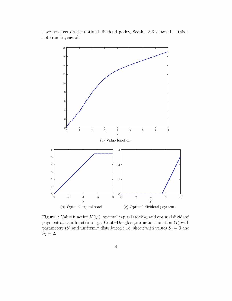
have no effect on the optimal dividend policy, Section 3.3 shows that this isnot true in general.

0 1 2 3 4 5 6 7 80

2

4

6

8

10

12

14

16

18

y

(a) Value function.

0 2 4 6 80

1

2

3

4

5

6

y

(b) Optimal capital stock.

0 2 4 6 80

1

2

3

y

(c) Optimal dividend payment.

Figure 1: Value function V (yt), optimal capital stock kt and optimal dividendpayment dt as a function of yt. Cobb–Douglas production function (7) withparameters (8) and uniformly distributed i.i.d. shock with values S1 = 0 andS2 = 2.

8

Dividend and investment policy. The optimal investment and divi-dend policy are depicted in Figures 1(b) and (c). The firm’s policy is simple:below a certain capital level, all earnings are reinvested and no dividendsare paid. If the output exceeds this threshold, then the capital stock is heldconstant and all ‘excess earnings’ are disbursed to the owners.

The threshold capital stock above which dividend payments are madeis given by k∗ = 5.48. This level is about 6.4% higher than the optimal(constant) capital stock of 5.15 which would be employed by a firm withoutfinancing constraints. The higher capital stock reduces bankruptcy risk andallows the firm to rebuild its capital faster and resume dividend paymentsearlier, after the occurrence of the shock S2. The firm’s policy can be in-terpreted as precautionary savings which enable the firm to (temporarily)mitigate the effect of the shock. Cooley and Quadrini (2001) find the sameinvestment policy in a model with default costs, costs of raising new capitaland shocks that are proportional to the firm’s output.

In our model firms hold capital above the socially optimal level and theiroptimal size is larger than if they had access to outside finance. Unlike inmodels with perfect capital markets such as Modigliani and Miller (1958)(where dividend payments can be offset by refinancing), the dividend pol-icy matters and precautionary savings are optimal. The optimal policy ofthe firm matches empirical observations on retained earnings. Fazzari et al.(1988) find that firms with a value below 10 million dollars (small firms) havea retention ratio of 79%, whereas firms with a value over one billion have aratio of 52%, i.e., smaller firms rely more on internal funding of investments.Guiso (1998), however, finds that size can be a poor proxy for measuringcredit constraints.

Precautionary savings are, in practice, often related to holding more liq-uid assets, Opler et al. (1999). Our model makes no distinction betweenliquid and illiquid assets but the firm holds more assets than if it were uncon-strained. Further evidence of precautionary savings is presented in Almeidaet al. (2004) who find that companies save a larger proportion of their cashflow in good times (when the cash flow is high) in order to realize investmentopportunities in times with low cash flows. This behavior closely resemblesthe precautionary savings observed in our model where the firm requirescapital to survive negative shocks.

The firm’s optimal dividend policy implies that larger companies paymore dividends and very small companies do not pay any. Fazzari et al.(1988) find that, in 1970, low dividend-paying firms were, on average, more

9

than 12 times smaller than the high dividend-paying firms and that firmswith low dividends, investments relative to capital are almost 50% higherthan for high dividend payers. More recent findings by Fama and French(2001), and Grullon et al. (2002) are similar. According to DeAngelo et al.(2006), in 2003, only 18.9% of the companies paid any dividends.

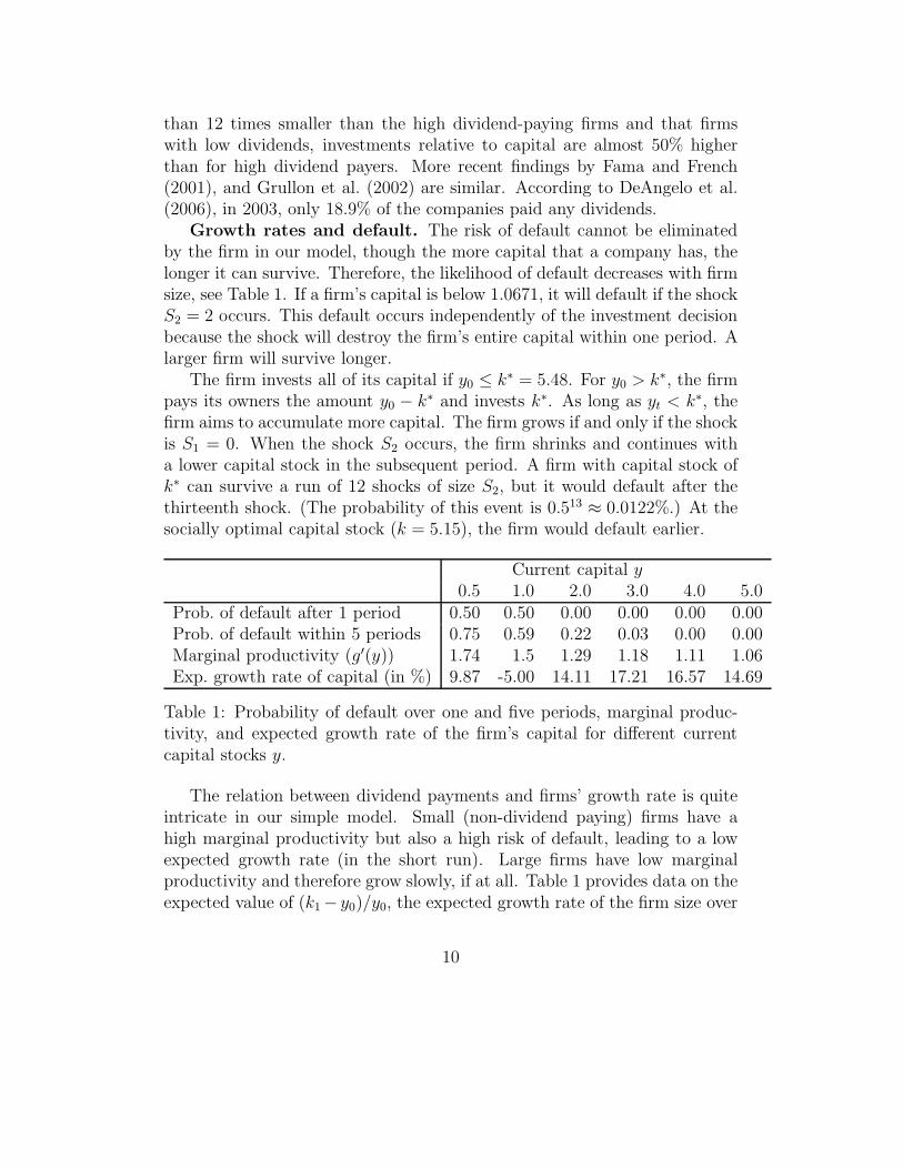
Growth rates and default. The risk of default cannot be eliminatedby the firm in our model, though the more capital that a company has, thelonger it can survive. Therefore, the likelihood of default decreases with firmsize, see Table 1. If a firm’s capital is below 1.0671, it will default if the shockS2 = 2 occurs. This default occurs independently of the investment decisionbecause the shock will destroy the firm’s entire capital within one period. Alarger firm will survive longer.

The firm invests all of its capital if y0 ≤ k∗ = 5.48. For y0 > k∗, the firmpays its owners the amount y0 − k∗ and invests k∗. As long as yt < k∗, thefirm aims to accumulate more capital. The firm grows if and only if the shockis S1 = 0. When the shock S2 occurs, the firm shrinks and continues witha lower capital stock in the subsequent period. A firm with capital stock ofk∗ can survive a run of 12 shocks of size S2, but it would default after thethirteenth shock. (The probability of this event is 0.513 ≈ 0.0122%.) At thesocially optimal capital stock (k = 5.15), the firm would default earlier.

Current capital y0.5 1.0 2.0 3.0 4.0 5.0

Prob. of default after 1 period 0.50 0.50 0.00 0.00 0.00 0.00Prob. of default within 5 periods 0.75 0.59 0.22 0.03 0.00 0.00Marginal productivity (g′(y)) 1.74 1.5 1.29 1.18 1.11 1.06Exp. growth rate of capital (in %) 9.87 -5.00 14.11 17.21 16.57 14.69

Table 1: Probability of default over one and five periods, marginal produc-tivity, and expected growth rate of the firm’s capital for different currentcapital stocks y.

The relation between dividend payments and firms’ growth rate is quiteintricate in our simple model. Small (non-dividend paying) firms have ahigh marginal productivity but also a high risk of default, leading to a lowexpected growth rate (in the short run). Large firms have low marginalproductivity and therefore grow slowly, if at all. Table 1 provides data on theexpected value of (k1 − y0)/y0, the expected growth rate of the firm size over

10

T = 1 period. (In our model, positive growth only happens in the absence ofthe negative shock S2.) Small as well as large companies experience fallinggrowth rates with increasing size. The growth rate of smaller firms is morevolatile because the the shock is independent of firm size; small firms areriskier than large firms.

Hall (1987), Evans (1987a,b) and Dhawan (2001) provide evidence, basedon US manufacturing firm data, that small firms grow quicker, are moreproductive and riskier than larger firms. Models with financing constraintstypically arrive at the same result, see, for example, Cooley and Quadrini(2001), Albuquerque and Hopenhayn (2004) and Clementi and Hopenhayn(2006).

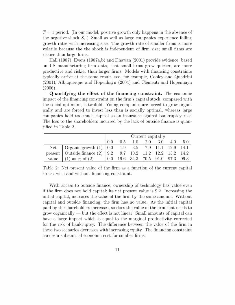
Quantifying the effect of the financing constraint. The economicimpact of the financing constraint on the firm’s capital stock, compared withthe social optimum, is twofold. Young companies are forced to grow organ-ically and are forced to invest less than is socially optimal, whereas largecompanies hold too much capital as an insurance against bankruptcy risk.The loss to the shareholders incurred by the lack of outside finance is quan-tified in Table 2.

Current capital y0.0 0.5 1.0 2.0 3.0 4.0 5.0

Net Organic growth (1) 0.0 1.9 3.5 7.9 11.1 12.9 14.1present Outside finance (2) 9.2 9.7 10.2 11.2 12.2 13.2 14.2value (1) as % of (2) 0.0 19.6 34.3 70.5 91.0 97.3 99.3

Table 2: Net present value of the firm as a function of the current capitalstock: with and without financing constraint.

With access to outside finance, ownership of technology has value evenif the firm does not hold capital; its net present value is 9.2. Increasing theinitial capital, increases the value of the firm by the same amount. Withoutcapital and outside financing, the firm has no value. As the initial capitalpaid by the shareholders increases, so does the value of the firm that needs togrow organically — but the effect is not linear. Small amounts of capital canhave a large impact which is equal to the marginal productivity correctedfor the risk of bankruptcy. The difference between the value of the firm inthese two scenarios decreases with increasing equity. The financing constraintcarries a substantial economic cost for smaller firms.

11

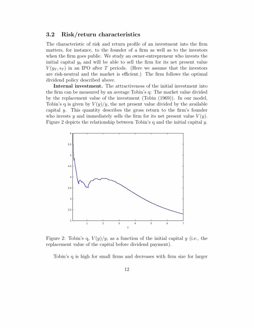
3.2 Risk/return characteristics

The characteristic of risk and return profile of an investment into the firmmatters, for instance, to the founder of a firm as well as to the investorswhen the firm goes public. We study an owner-entrepreneur who invests theinitial capital y0 and will be able to sell the firm for its net present valueV (yT , sT ) in an IPO after T periods. (Here we assume that the investorsare risk-neutral and the market is efficient.) The firm follows the optimaldividend policy described above.

Internal investment. The attractiveness of the initial investment intothe firm can be measured by an average Tobin’s q: The market value dividedby the replacement value of the investment (Tobin (1969)). In our model,Tobin’s q is given by V (y)/y, the net present value divided by the availablecapital y. This quantity describes the gross return to the firm’s founderwho invests y and immediately sells the firm for its net present value V (y).Figure 2 depicts the relationship between Tobin’s q and the initial capital y.

1 2 3 4 5 6 72

2.5

3

3.5

4

4.5

5

5.5

6

y

Figure 2: Tobin’s q, V (y)/y, as a function of the initial capital y (i.e., thereplacement value of the capital before dividend payment).

Tobin’s q is high for small firms and decreases with firm size for larger

12

capital stocks, though it is always larger than 1. Firms with a high Tobin’sq reinvest all earnings, whereas those with a low Tobin’s q pay dividends.The scope for expected future income, which can be realized with retainedearnings, gives small firms a high value relative to its capital. Relative tothe socially optimal size they are too small and the financing constraint bitsparticularly hard. These observations are in lines with findings by Fazzariet al. (1988) and Erickson and Whited (2000) who show that constrainedUS firms have a higher Tobin’s q and that these firms invest more. Theseproperties also correspond to the simulation results presented in Cooley andQuadrini (2001).

For intermediate firm sizes, the non-concavity of the value function (owingto bankruptcy risk) implies a rather complex relationship which implies that,even in simple models, the relation between size and Tobin’s q is not trivial.This puts into perspective the difficulties in finding strong empirical relationsbetween Tobin’s q and investment.

Outside investment. The return to a stock market investor who par-ticipates in the IPO is measured by the annualized ratio of the firm’s netpresent value at time T and the ex-dividend net present value at time 0:

RT (y0, sT ) =

(

V (yT (sT ))

V (y0) − d0

)1/T

, (9)

where yT (sT ) is the output in period T , which is determined by the sequenceof shocks sT = (s1, . . . , sT ) and the firm’s optimal dividend policy. The meanand variance of the return are given by

µT (y0) =∑

sT∈ST

p(sT )RT (y0, sT )

andσT (y0)

2 =∑

sT ∈ST

p(sT )(RT (y0, sT ) − µT (y0))

2,

where p(sT ) = πs1· · ·πsT

is the probability of observing the sequence ofshocks sT .

Empirical evidence of Whited and Wu (2006) and the simulation resultsof Livdan et al. (2009) suggest that, on average, more constrained firms havehigher returns and higher volatility. In our model this holds only for verysmall firms. For example, if T = 5, the initial capital must be below y0 =

13

0.902 which gives very unattractive expected return below µT = 0.44317.Indeed, the return-volatility profile improves for investments up to y0 = 3.617where µT = 1.02608 and σT = 0.05425. For higher initial investments, therelation between the expected return and volatility follows the classical mean-variance diagram.

0 5 10 150

0.1

0.2

0.3

0.4

0.5

0.6

Market Value

Vola

tility

of R

etu

rn

y0 = k∗

uEEEEE

y0 = 0.1

u

(a) Market value and expected return.

3 4 5 60

0.2

0.4

0.6

0.8

1

Market-to-Book-Ratio

Exp

ect

ed R

etu

rn

y0 = k∗

u

y0 = 0.1

u

(b) Market-to-book ratio and expectedreturn.

Figure 3: Expected return µT (y0) over T = 5 periods as a function of thefirm’s, market value V (y0) (panel (a)) and its market-to-book ratio V (y0)/y0

(panel (b)). Each point on the graphs corresponds to a particular initialcapital stock y0 with y0 = n · 10−3, n an integer and 0.1 ≤ y0 ≤ k∗ = 5.48.

Leverage effect. As the company does not issue new capital, the marketvalue of the firm is equal to its equity price and, therefore, some observationson equity returns can be made. Figure 3(a) presents the volatility of stockmarket returns, defined in (9), as a function of the value of the firm (i.e.,its market capitalization). For large firms, volatility decreases with marketcapitalization. This effect is reversed for smaller firms with a value below3.2240. Higher volatility as a result of falling equity prices, as observedfor the large companies in Figure 3(a), is a stylized fact called the leverageeffect. Black (1976) argues that a drop in the value of a company increases itsleverage and, therefore, makes it riskier. Christie (1982) and Schwert (1989)show that volatility is an increasing function of leverage. The simulation

14

results by Livdan et al. (2009) also show that financially constrained firmshave a higher systematic risk.

Another possible explanation of the leverage effect is that a permanentincrease in volatility increases, leads shareholders to demand a higher averagereturn; therefore, today’s price has to fall. This point is made, e.g., byPindyck (1984), French et al. (1987), Turner et al. (1989), Campbell andHentschel (1992), Wu (2001), Kim et al. (2004) and Mayfield (2004). Bekaertand Wu (2000) and Bae et al. (2007) quantify both effects in a model andfind that the second effect is stronger. Since in the present model there isneither a risk premium nor leverage, our results show that these effects canbe caused by financial constraints: A less valuable company becomes riskierbecause the likelihood of default increases if there is less capital to absorbshocks.

Value premium. The book value of a firm is the replacement valueof the assets that the company owns. The market-to-book value ratio isan indicator of whether the company is a so-called ‘growth’ company or a‘value’ company. A growth company (high market-to-book value) has fewassets now, but the market expects the company to grow quickly and deliversubstantial profit in the future. Value companies (low market-to-book value)already have many assets today, and their growth expectations are lower.Figure 3(b) illustrates the relation between the market-to-book ratio andexpected returns in our model.

Firms with a low market-to-book value have a high capital stock but theyalso have high expected returns. The maximum expected return of 1.02608 isattained at a market-to-book ratio of 3.40557. Companies with little initialcapital have a high market-to-book value but low returns and, by and large,the returns increase with a higher market-to-book ratio (see Figure 3(b)).This property is in line with the empirical findings by Stattman (1980),Rosenberg et al. (1985) and Chan et al. (1991). Fama and French (1992, 1998)and others found (using US and international data) that value stocks performbetter than growth stocks, and that this effect cannot be explained by marketrisk factors. It is often argued that the premium for value stocks (i.e., stockswith a low book-to-market value) reflects other risk factors. In that view,the value premium is an indicator of the investment opportunities in theeconomy.4 Our model shows (as also observed by Livdan et al. (2009)) that

4E.g., Fama and French (1996), Liew and Vassalou (2000), Campbell and Vuolteenaho(2004), Brennan et al. (2004), Hahn and Lee (2006) and Petkova (2006) or, for equilibrium

15

these considerations are not needed if there are financial constraints. Highmarket-to-book ratios may just be an indicator for financially constrainedfirms that also face a higher default risk, such that expected returns arelower.

3.3 Multiple i.i.d. shocks

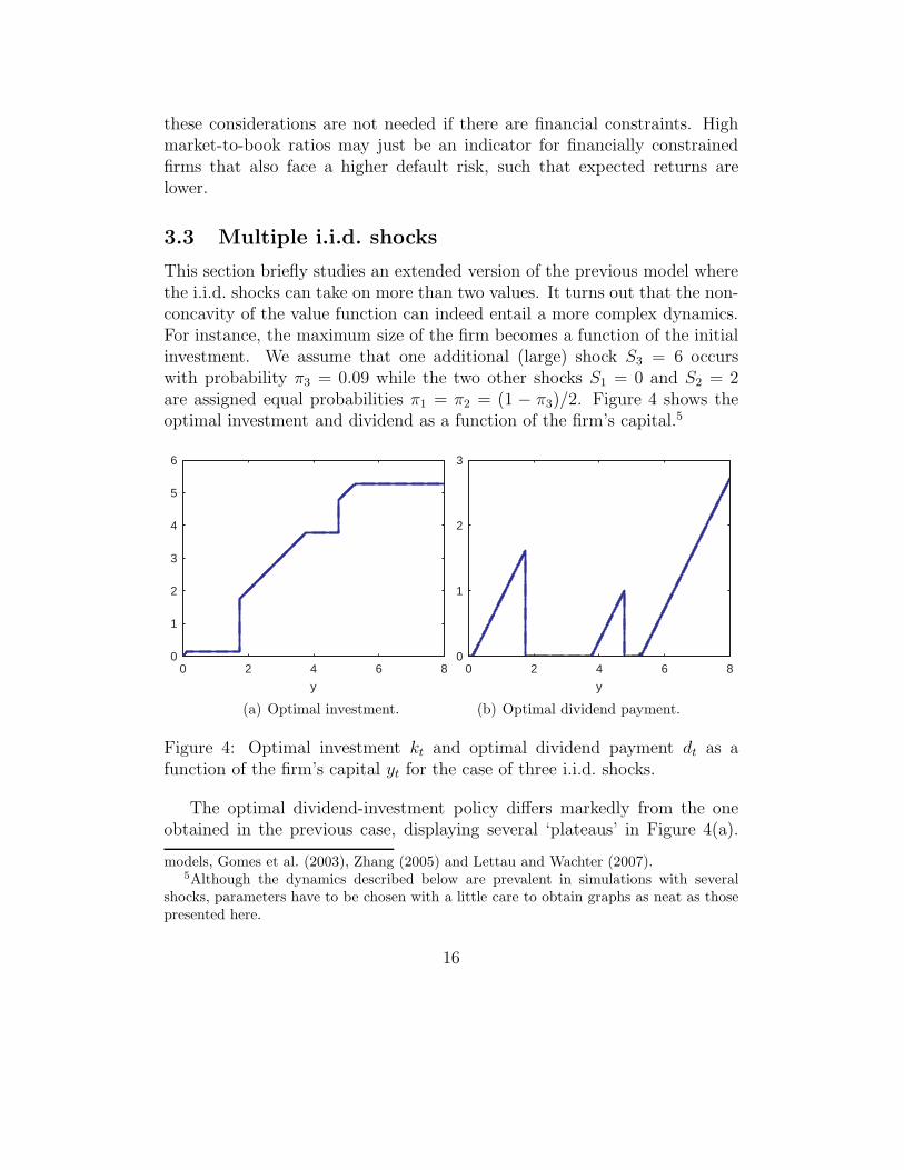
This section briefly studies an extended version of the previous model wherethe i.i.d. shocks can take on more than two values. It turns out that the non-concavity of the value function can indeed entail a more complex dynamics.For instance, the maximum size of the firm becomes a function of the initialinvestment. We assume that one additional (large) shock S3 = 6 occurswith probability π3 = 0.09 while the two other shocks S1 = 0 and S2 = 2are assigned equal probabilities π1 = π2 = (1 − π3)/2. Figure 4 shows theoptimal investment and dividend as a function of the firm’s capital.5

0 2 4 6 80

1

2

3

4

5

6

y

(a) Optimal investment.

0 2 4 6 80

1

2

3

y

(b) Optimal dividend payment.

Figure 4: Optimal investment kt and optimal dividend payment dt as afunction of the firm’s capital yt for the case of three i.i.d. shocks.

The optimal dividend-investment policy differs markedly from the oneobtained in the previous case, displaying several ‘plateaus’ in Figure 4(a).

models, Gomes et al. (2003), Zhang (2005) and Lettau and Wachter (2007).5Although the dynamics described below are prevalent in simulations with several

shocks, parameters have to be chosen with a little care to obtain graphs as neat as thosepresented here.

16

In the present example there are three distinctive plateaus at different levelsof capital stocks: low (k∗

l = 0.128), medium (k∗m = 3.766) and high (k∗

h =5.283). Each of these plateaus corresponds to a capital level above whichthe firm starts paying dividends. A firm with a capital stock below k∗

l paysout all earnings exceeding k∗

l and maintains this size until the shock S2 orS3 causes it to go bankrupt. The level k∗

h corresponds to the maximum sizeto which a firm can grow organically with an initial capital of y∗

h = 1.739or more. For a capital level below y∗

h, the firm size converges to an optimalcapital level of k∗

l . If the initial endowment is on the medium plateau betweenk∗

m and k∗m = 4.761, the firm will pay dividends of y− k∗

m and shrinks to sizek∗

m. If there is no negative shock (i.e., S1 = 0 is realized), the company willgrow in the next period from k∗

m directly to k∗h. Therefore, the effect of the

medium level typically occurs only for one period. A firm of size k∗h will retain

earnings after one shock of size S2, with the aim of reaching its previous size.If the large shock S3 is realized, however, the capital stock falls below y∗

h andthe firm will not grow to its previous size but rather shrink to size k∗

l .

4 Business cycles and optimal investment

The business cycle has a significant impact on firms’ optimal dividend-invest-ment policies. In this section we aim to study its effect within the frameworkof our model. The business cycle is implemented as exogenous market condi-tions with a certain degree of persistence, modeled by a Markov process withtwo shocks S1 = 0 (boom) and S2 = 2 (recession) and (symmetric) transi-tion probabilities π11 = π22 = p. The probability of a change of the regimeis given by π12 = π21 = 1 − p. The higher p, the higher is the persistence ofa state and, thus, the average duration of regimes. The value function andthe optimal policy of the firm will depend on the current state of the shock.

We are interested in qualitative differences in the firm’s optimal policybetween booms and recessions and, in particular, the effect of the duration ofrecessions (measured by p) and the depth (varying S2) on the firm’s optimalpolicy. The production function and parameters are given by (7)–(8) andare identical to the case studied in Section 3 (which is obtained by settingp = 0.5).

17

4.1 Optimal dividend-investment policy

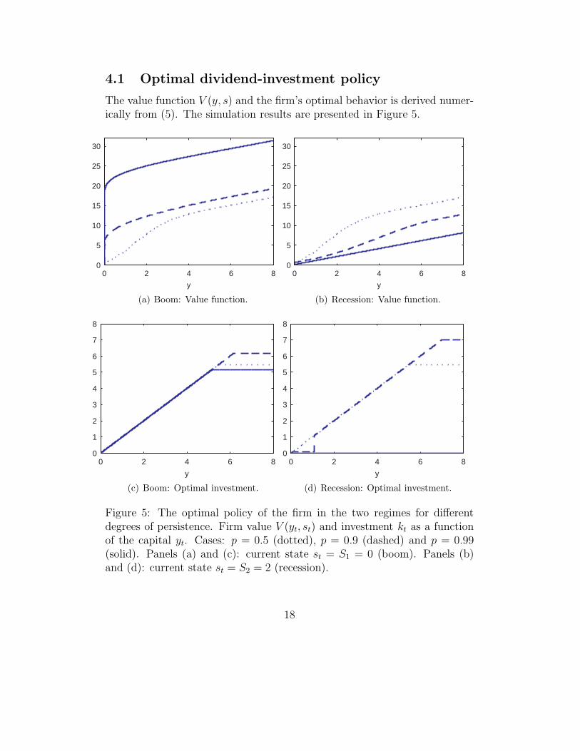
The value function V (y, s) and the firm’s optimal behavior is derived numer-ically from (5). The simulation results are presented in Figure 5.

0 2 4 6 80

5

10

15

20

25

30

y

(a) Boom: Value function.

0 2 4 6 80

5

10

15

20

25

30

y

(b) Recession: Value function.

0 2 4 6 80

1

2

3

4

5

6

7

8

y

(c) Boom: Optimal investment.

0 2 4 6 80

1

2

3

4

5

6

7

8

y

(d) Recession: Optimal investment.

Figure 5: The optimal policy of the firm in the two regimes for differentdegrees of persistence. Firm value V (yt, st) and investment kt as a functionof the capital yt. Cases: p = 0.5 (dotted), p = 0.9 (dashed) and p = 0.99(solid). Panels (a) and (c): current state st = S1 = 0 (boom). Panels (b)and (d): current state st = S2 = 2 (recession).

18

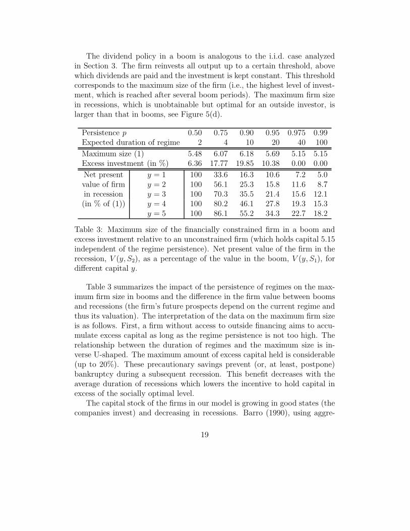
The dividend policy in a boom is analogous to the i.i.d. case analyzedin Section 3. The firm reinvests all output up to a certain threshold, abovewhich dividends are paid and the investment is kept constant. This thresholdcorresponds to the maximum size of the firm (i.e., the highest level of invest-ment, which is reached after several boom periods). The maximum firm sizein recessions, which is unobtainable but optimal for an outside investor, islarger than that in booms, see Figure 5(d).

Persistence p 0.50 0.75 0.90 0.95 0.975 0.99Expected duration of regime 2 4 10 20 40 100

Maximum size (1) 5.48 6.07 6.18 5.69 5.15 5.15Excess investment (in %) 6.36 17.77 19.85 10.38 0.00 0.00

Net present y = 1 100 33.6 16.3 10.6 7.2 5.0value of firm y = 2 100 56.1 25.3 15.8 11.6 8.7in recession y = 3 100 70.3 35.5 21.4 15.6 12.1(in % of (1)) y = 4 100 80.2 46.1 27.8 19.3 15.3

y = 5 100 86.1 55.2 34.3 22.7 18.2

Table 3: Maximum size of the financially constrained firm in a boom andexcess investment relative to an unconstrained firm (which holds capital 5.15independent of the regime persistence). Net present value of the firm in therecession, V (y, S2), as a percentage of the value in the boom, V (y, S1), fordifferent capital y.

Table 3 summarizes the impact of the persistence of regimes on the max-imum firm size in booms and the difference in the firm value between boomsand recessions (the firm’s future prospects depend on the current regime andthus its valuation). The interpretation of the data on the maximum firm sizeis as follows. First, a firm without access to outside financing aims to accu-mulate excess capital as long as the regime persistence is not too high. Therelationship between the duration of regimes and the maximum size is in-verse U-shaped. The maximum amount of excess capital held is considerable(up to 20%). These precautionary savings prevent (or, at least, postpone)bankruptcy during a subsequent recession. This benefit decreases with theaverage duration of recessions which lowers the incentive to hold capital inexcess of the socially optimal level.

The capital stock of the firms in our model is growing in good states (thecompanies invest) and decreasing in recessions. Barro (1990), using aggre-

19

gated US investment data, shows that investment is pro-cyclical. Defaults inour model happen only in a recession which mimics the empirical fact thatdefault probabilities are larger in periods of falling stock prices (Vassalou andXing (2004) and Chava and Jarrow (2004)) which coincide with falling GDP(Chen (2010)).

The effect of regime duration on the variation of the firm value betweenbooms and recessions is as follows, see Table 3. Smaller firms are harder hitby a recession. Whereas a large company will only lose about one-third ofits value when entering a recession that lasts on average 10 periods, a smallfirm will see its value decline to 16.3%. This is caused by the low chances ofsurvival in a persistent recession when the firm has little capital.

It is more attractive for an outside investor to invest during booms (sincethe same amount of capital y delivers a higher value V (y, S0) > V (y, S1)),implying that new companies will be founded mainly during booms. Thisfeature matches the waves of IPOs documented by Ibbotson and Jaffe (1975)and Pastor and Veronesi (2005) who show that IPOs are more frequent inrising stock markets. A pro-cyclical pattern of firms’ output, entry and exitis also found in the computational study by Delli Gatti et al. (2003). In theirmodel firms face quadratic adjustment cost of capital and exogenously spec-ified dividends. Companies default, if they are not able to pay the intereston their debts.

4.2 Effect of the depth of recession

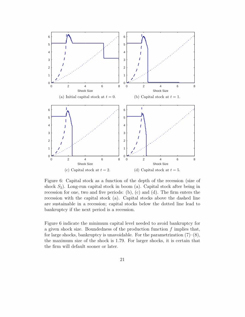
We next study the effect of the depth of the recession on the firm’s optimaldividend-investment policy. The depth is given by the size of the shock S2

which will be varied in what follows (we set p = 0.9 and S1 = 0).Bankruptcy eventually happens irrespective of the firm’s policy if the

shock is larger then the threshold S2 > 1.79. For a smaller shock (S2 ≤ 1.79),there are sustainable levels of capital, i.e., f(k, S2) ≥ k. The size of the shockaffects the firm’s behavior during recessions as well as booms. Figure 6 showsthe evolution of the firm’s capital stock over time during a recession lastingfive periods with the depth of the recession as a parameter. We assume thatthe firm enters the recession with the maximum capital level that it wouldattain in a boom.

The maximum size of the firm depends on the depth of the recession, asshown in Figure 6 (a). A company survives a recession of arbitrary length aslong as its capital stock k is sustainable in a recession. The dashed lines in

20

0 2 4 6 80

1

2

3

4

5

6

Shock Size

(a) Initial capital stock at t = 0.

0 2 4 6 80

1

2

3

4

5

6

Shock Size

(b) Capital stock at t = 1.

0 2 4 6 80

1

2

3

4

5

6

Shock Size

(c) Capital stock at t = 2.

0 2 4 6 80

1

2

3

4

5

6

Shock Size

(d) Capital stock at t = 5.

Figure 6: Capital stock as a function of the depth of the recession (size ofshock S2). Long-run capital stock in boom (a). Capital stock after being inrecession for one, two and five periods: (b), (c) and (d). The firm enters therecession with the capital stock (a). Capital stocks above the dashed lineare sustainable in a recession; capital stocks below the dotted line lead tobankruptcy if the next period is a recession.

Figure 6 indicate the minimum capital level needed to avoid bankruptcy fora given shock size. Boundedness of the production function f implies that,for large shocks, bankruptcy is unavoidable. For the parametrization (7)–(8),the maximum size of the shock is 1.79. For larger shocks, it is certain thatthe firm will default sooner or later.

21

For smaller shock sizes, S2 ≤ 1.79, the firm accumulates capital up tothe socially optimal level of 5.15 and, at this level, does not face any risk ofbankruptcy. If the shock S2 is larger, the firm holds more capital in booms.Holding this ‘excess’ capital reduces the risk of bankruptcy by postponingeventual bankruptcy during a recession because the firm has a capital buffer.This is illustrated in Figure 6 (b)–(d) by the ‘hump’ in the graph, whichis located at shocks of size 1.76 ≤ S2 ≤ 2.48. The excess capital held bythe firm first increases and then decreases with the depth of the recession.These precautionary savings are optimal because additional capital helps topostpone bankruptcy by many periods if the shock is just above the threshold1.76. As the shock becomes larger, more excess capital is required to obtainthe same benefit. At some shock size (here 2.12), the costs start to outweighthe benefit, leading to lower precautionary savings.

If the shock size S2 is larger than 2.48, the firm does not hold any excesscapital in booms but rather chooses to accumulate capital up to the sociallyoptimal level. When entering a recession, the firm pays out almost all ofits remaining capital and keeps only a very small amount, which ensuressurvival only if a boom follows in the next period. Without instantaneousrecovery, the firm will be bankrupt. If shocks are even more extreme (suchthat they would lead to the destruction of all of the firm’s capital in oneperiod of recession), the maximum size of the firm is 3.18. The inability tosurvive recessions induces firms to limit their size in the boom phase belowthe socially optimal one. This optimal behavior is evidenced as the downwardstep observed in Figure 6 (a) (and, although less visibly, in panel (b)).

5 Optimal policy of the central bank

We finally study the impact of the interest rate set by a central bank inresponse to prevailing economic conditions. The central bank is not ableto anticipate the regime prevailing in the next period, but has to choosethe interest rate r(st) as a function of the currently observed state st. Wedenote by r1 := r(S1) resp. r2 := r(S2) the interest rate set in a boomresp. recession. (The policy will always lag the state of the economy by oneperiod). We further assume that there is a given average interest rate r∗

that the bank has to meet. In the symmetric case where, on average, boomsand recessions last for the same number of periods, this condition can bewritten as (1 + r1)(1 + r2) = (1 + r∗)2. We will use the same specification of

22

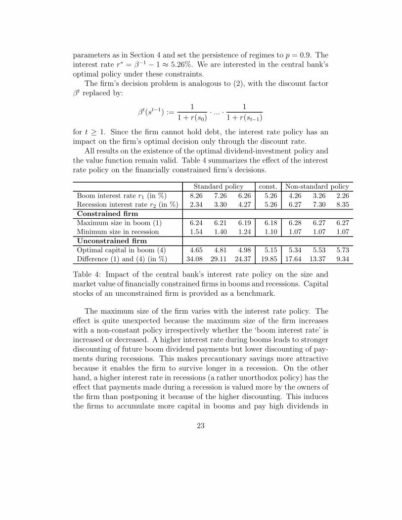
parameters as in Section 4 and set the persistence of regimes to p = 0.9. Theinterest rate r∗ = β−1 − 1 ≈ 5.26%. We are interested in the central bank’soptimal policy under these constraints.

The firm’s decision problem is analogous to (2), with the discount factorβt replaced by:

βt(st−1) :=1

1 + r(s0)· ... ·

1

1 + r(st−1)

for t ≥ 1. Since the firm cannot hold debt, the interest rate policy has animpact on the firm’s optimal decision only through the discount rate.

All results on the existence of the optimal dividend-investment policy andthe value function remain valid. Table 4 summarizes the effect of the interestrate policy on the financially constrained firm’s decisions.

Standard policy const. Non-standard policy

Boom interest rate r1 (in %) 8.26 7.26 6.26 5.26 4.26 3.26 2.26Recession interest rate r2 (in %) 2.34 3.30 4.27 5.26 6.27 7.30 8.35

Constrained firm

Maximum size in boom (1) 6.24 6.21 6.19 6.18 6.28 6.27 6.27Minimum size in recession 1.54 1.40 1.24 1.10 1.07 1.07 1.07

Unconstrained firm

Optimal capital in boom (4) 4.65 4.81 4.98 5.15 5.34 5.53 5.73Difference (1) and (4) (in %) 34.08 29.11 24.37 19.85 17.64 13.37 9.34

Table 4: Impact of the central bank’s interest rate policy on the size andmarket value of financially constrained firms in booms and recessions. Capitalstocks of an unconstrained firm is provided as a benchmark.

The maximum size of the firm varies with the interest rate policy. Theeffect is quite unexpected because the maximum size of the firm increaseswith a non-constant policy irrespectively whether the ‘boom interest rate’ isincreased or decreased. A higher interest rate during booms leads to strongerdiscounting of future boom dividend payments but lower discounting of pay-ments during recessions. This makes precautionary savings more attractivebecause it enables the firm to survive longer in a recession. On the otherhand, a higher interest rate in recessions (a rather unorthodox policy) has theeffect that payments made during a recession is valued more by the owners ofthe firm than postponing it because of the higher discounting. This inducesthe firms to accumulate more capital in booms and pay high dividends in

23

recessions, entailing an extremely high bankruptcy risk. The excess capitalstock (last row in Table 4) held by the financially constrained firms in goodtimes (booms) is increasing the lower the interest rate is set in recessions.

The minimum size (defined here as smallest the capital stock at whichthe firm chooses to continue operations in a recession rather than payingout almost all remaining capital) increases when the recession interest ratedecreases. The effect of this standard interest rate policy, however, is drivenby the high boom interest rate. In a recession the firm does not pay anydividends, their payment is only resumed in a boom which makes the capitalholdings at the end of a recession more valuable. The firm therefore holdson to a higher capital stock in a recession.

Summarizing, the standard policy of low interest rates in recessions givesfinancially constrained firms an incentive to retain more of its earnings ingood times (booms) and to stay longer in business in bad times (recession).In this sense, investments happen in booms out of precautionary motives.The persistence of regimes plays a vital role in the firm’s decision, in thepresence of i.i.d. shocks no adjustment to the business cycle would occur.

In the theoretical models of Bernanke and Gertler (1989), Kiyotaki andMoore (1997) and Carlstrom and Fuerst (1997), firms with limited access tothe credit market (due to information asymmetries) cannot finance profitableinvestments because of macroeconomic shocks which reduce the value of thefirms’ collateral. The presence of this investment pattern is confirmed empir-ically by Gertler and Gilchrist (1994) and Bernanke et al. (1996). Monetarypolicy is found by Cooley and Quadrini (2006) to have a stronger (in termsof output and debts) impact of financially constrained small firms.

In our model, in contrast, financially constrained firms reduce their in-vestment less than unconstrained firms at the outset of a recession becausethey accumulated precautionary savings in the previous boom. However, ourresults are about a different type of firm (those that do not have any accessto credit) and, in addition, firms face persistent (rather than i.i.d.) shocks.We would argue that precautionary saving motives of financially constrainedfirm are more important under persistent recession regimes.

6 Conclusions

This paper studies the optimal behavior of a financially constrained firmin the presence of additive production shocks. The model is one of pure

24

capital accumulation under i.i.d. as well as Markov (business cycle) shocks.Several stylized economic and financial characteristics of the firm life cyclecan be illustrated within this simple model. The dynamic captures the higherdefault risk, productivity and volatility of small firms, the concentration ofdividend payments on large firms, a falling Tobin’s q in firm size, the leverageeffect, the value premium, the pro-cyclically investment and firm entries, andcounter-cyclical default probabilities. We also study the impact of a centralbank’s interest policy on firms’ precautionary savings and their optimal size.

The approach offers several avenues for future research without losingmuch of the simplicity of the model. It would be interesting to weaken the(extreme) assumption of lack of access to any outside finance by allowingfirms to raise at least some capital from, e.g., venture capitalists. The as-sumption on the risk-neutrality of the owner-entrepreneur can be replacedby other (neoclassical or behavioral) preferences. One could also study theimpact of a proportional shock in the presence of fixed costs rather thanimposing an additive output shock as in our model. Finally, competition ofseveral firms in an output market (with some stochastic aggregate demandfunction) can also be studied in a generalized model.

References

Albuquerque, R., Hopenhayn, H.A., 2004. Optimal Lending Contracts and FirmDynamics. Review of Economic Studies 71, 285–315.

Almeida, H., Campello, M., Weisbach, M.S., 2004. The Cash Flow Sensitivity ofCash. Journal of Finance 59, 1777–1804.

Bae, J., Kim, C.J., Nelson, C.R., 2007. Why Are Stock Returns and VolatilityNegatively Correlated? Journal of Empirical Finance 14, 41–58.

Barro, R.J., 1990. The Stock Market and Investment. Review of Financial Studies3, 115–131.

Bekaert, G., Wu, G., 2000. Asymmetric Volatility and Risk in Equity Markets.Review of Financial Studies 13, 1–42.

Bernanke, B., Gertler, M., Gilchrist, S., 1996. The Financial Accelerator and theFlight to Quality. Review of Economics and Statistics 78, 1–15.

Bernanke, B.S., Gertler, M., 1989. Agency Costs, Net Worth, and Business Fluc-tuations. American Economic Review 79, 14–31.

25

Black, F., 1976. Studies of Stock Price Volatility Changes. Proceedings of the Meet-ings of the American Statistical Association, Business and Economics StatisticsDivision, 177–181.

Brennan, M.J., Wang, A.W., Xia, Y., 2004. Estimation and Test of a Simple Modelof Intertemporal Capital Asset Pricing. Journal of Finance 59, 1743–1775.

Campbell, J.Y., Hentschel, L., 1992. No News is Good News: An AsymmetricModel of Changing Volatility in Stock Returns. Journal of Financial Economics31, 281–318.

Campbell, J.Y., Vuolteenaho, T., 2004. Bad Beta, Good Beta. American EconomicReview 94, 1249–1275.

Carlstrom, C.T., Fuerst, T.S., 1997. Agency Costs, Net Worth, and Business Fluc-tuations: A Computable General Equilibrium Analysis. American EconomicReview 87, 893–910.

Chan, L.K.C., Hamao, Y., Lakonishok, J., 1991. Fundamentals and Stock Returnsin Japan. Journal of Finance 46, 1739–1764.

Chava, S., Jarrow, R.A., 2004. Bankruptcy Prediction with Industry Effects.Review of Finance 8, 537–569.

Chen, H., 2010. Macroeconomic Conditions and the Puzzles of Credit Spreads andCapital Structure. Journal of Finance, forthcoming.

Christie, A.A., 1982. The Stochastic Behavior of Common Stock Variances : Value,Leverage and Interest Rate Effects. Journal of Financial Economics 10, 407–432.

Clementi, G.L., Hopenhayn, H.A., 2006. A Theory of Financing Constraints andFirm Dynamics. Quarterly Journal of Economics 121, 229–265.

Cooley, T.F., Quadrini, V., 2001. Financial Markets and Firm Dynamics. Ameri-can Economic Review 91, 1286–1310.

Cooley, T.F., Quadrini, V., 2006. Monetary Policy and the Financial Decisions ofFirms. Economic Theory 27, 243–270.

DeAngelo, H., DeAngelo, L., Stulz, R.M., 2006. Dividend Policy and the Earned /Contributed Capital Mix: A Test of the Life-Cycle Theory. Journal of FinancialEconomics 81, 227–254.

26

Delli Gatti, D., Gallegati, M., Giulioni, G., Palestrini, A., 2003. Financial Fragility,Patterns of Firms’ Entry and Exit and Aggregate Dynamics. Journal of Eco-nomic Behavior & Organization 51, 79–97.

Dhawan, R., 2001. Firm Size and Productivity Differential: Theory and Evidencefrom a Panel of US Firms. Journal of Economic Behavior & Organization 44,269–293.

Dunne, T., Roberts, M.J., Samuelson, L., 1989. The Growth and Failure of U.S.Manufacturing Plants. Quarterly Journal of Economics 104, 671–698.

Erickson, T., Whited, T.M., 2000. Measurement Error and the Relationship be-tween Investment and ”q”. Journal of Political Economy 108, 1027–1057.

Evans, D.S., 1987a. Tests of Alternative Theories of Firm Growth. Journal ofPolitical Economy 95, 657–674.

Evans, D.S., 1987b. The Relationship between Firm Growth, Size, and Age: Es-timates for 100 Manufacturing Industries. Journal of Industrial Economics 35,567–581.

Fama, E.F., French, K.R., 1992. The Cross-Section of Expected Stock Returns.Journal of Finance 47, 427–465.

Fama, E.F., French, K.R., 1996. Multifactor Explanations of Asset Pricing Anoma-lies. Journal of Finance 51, 55–84.

Fama, E.F., French, K.R., 1998. Value versus Growth: The International Evidence.Journal of Finance 53, 1975–1999.

Fama, E.F., French, K.R., 2001. Disappearing Dividends: Changing Firm Char-acteristics or Lower Propensity to Pay? Journal of Financial Economics 60,3–43.

Fazzari, S.M., Hubbard, R.G., Petersen, B.C., 1988. Financing Constraints andCorporate Investment. Brookings Papers on Economic Activity 1, 141–195.

French, K.R., Schwert, G.W., Stambaugh, R.F., 1987. Expected Stock Returnsand Volatility. Journal of Financial Economics 19, 3–29.

Gertler, M., Gilchrist, S., 1994. Monetary Policy, Business Cycles, and the Be-havior of Small Manufacturing Firms. Quarterly Journal of Economics 109,309–340.

27

Gomes, J., Kogan, L., Zhang, L., 2003. Equilibrium Cross Section of Returns.Journal of Political Economy 111, 693–732.

Gort, M., Klepper, S., 1982. Time Paths in the Diffusion of Product Innovations.Economic Journal 92, 630–653.

Greenwald, B., Stiglitz, J.E., Weiss, A., 1984. Informational Imperfections in theCapital Market and Macroeconomic Fluctuations. American Economic Review74, 194–199.

Grossman, S.J., Hart, O.D., 1982. Corporate Financial Structure and ManagerialIncentives, in: The Economics of Information and Uncertainty. National Bureauof Economic Research, Inc. NBER Chapters, pp. 107–140.

Grullon, G., Michaely, R., Swaminathan, B., 2002. Are Dividend Changes a Signof Firm Maturity? Journal of Business 75, 387–424.

Guiso, L., 1998. High-tech Firms and Credit Rationing. Journal of EconomicBehavior & Organization 35, 39–59.

Hahn, J., Lee, H., 2006. Yield Spreads as Alternative Risk Factors for Size andBook-to-Market. Journal of Financial & Quantitative Analysis 41, 245–269.

Hall, B.H., 1987. The Relationship between Firm Size and Firm Growth in theU.S. Manufacturing Sector. Journal of Industrial Economics 35, 583–606.

Ibbotson, R.G., Jaffe, J.F., 1975. ”Hot Issue” Markets. Journal of Finance 30,1027–1042.

Jensen, M.C., 1986. Agency Costs of Free Cash Flow, Corporate Finance, andTakeovers. American Economic Review 76, 323–329.

Jensen, M.C., Meckling, W.H., 1976. Theory of the Firm: Managerial Behavior,Agency Costs and Ownership Structure. Journal of Financial Economics 3,305–360.

Jovanovic, B., 1982. Selection and the Evolution of Industry. Econometrica 50,649–670.

Kim, C.J., Morley, J.C., Nelson, C.R., 2004. Is There a Positive Relationshipbetween Stock Market Volatility and the Equity Premium? Journal of Money,Credit and Banking 36, 339–360.

28

Kiyotaki, N., Moore, J., 1997. Credit Cycles. Journal of Political Economy 105,211–248.

Klepper, S., 1996. Entry, Exit, Growth, and Innovation over the Product LifeCycle. American Economic Review 86, 562–583.

Lettau, M., Wachter, J.A., 2007. Why Is Long-Horizon Equity Less Risky? ADuration-Based Explanation of the Value Premium. Journal of Finance 62,55–92.

Liew, J., Vassalou, M., 2000. Can Book-to-Market, Size and Momentum Be RiskFactors that Predict Economic Growth? Journal of Financial Economics 57,221–245.

Livdan, D., Sapriza, H., Zhang, L., 2009. Financially Constrained Stock Returns.Journal of Finance 64, 1827–1862.

Martinelli, C., 1997. Small Firms, Borrowing Constraints, and Reputation. Journalof Economic Behavior & Organization 33, 91–105.

Mayfield, S., 2004. Estimating the Market Risk Premium. Journal of FinancialEconomics 73, 465–496.

Modigliani, F., Miller, M.H., 1958. The Cost of Capital, Corporation Finance andthe Theory of Investment. American Economic Review 48, 261–297.

Mueller, D.C., 1972. A Life Cycle Theory of the Firm. Journal of IndustrialEconomics 20, 199–219.

Mueller, D.C., Tilton, J.E., 1969. Research and Development Costs as a Barrierto Entry. Canadian Journal of Economics / Revue Canadienne d’Economique2, 570–579.

Myers, S.C., Majluf, N.S., 1984. Corporate Financing and Investment Decisionswhen Firms Have Information that Investors Do not Have. Journal of FinancialEconomics 13, 187–221.

Opler, T., Pinkowitz, L., Stulz, R., Williamson, R., 1999. The Determinants andImplications of Corporate Cash Holdings. Journal of Financial Economics 52,3–46.

Pastor, L., Veronesi, P., 2005. Rational IPO Waves. Journal of Finance 60, 1713–1757.

29

Petkova, R., 2006. Do the Fama-French Factors Proxy for Innovations in PredictiveVariables? Journal of Finance 61, 581–612.

Pindyck, R.S., 1984. Risk, Inflation, and the Stock Market. American EconomicReview 74, 335–351.

Riddick, L.A., Whited, T.M., 2009. The Corporate Propensity to Save. Journalof Finance 64, 1729–1766.

Rosenberg, B., Reid, K., Lanstein, R., 1985. Persuasive Evidence of Market Inef-ficiency. Journal of Portfolio Management 11, 9–16.

Schwert, G.W., 1989. Why Does Stock Market Volatility Change Over Time?Journal of Finance 44, 1115–1153.

Stattman, D., 1980. Book Values and Stock Returns. Chicago MBA: A Journalof Selected Papers 4, 25–45.

Stiglitz, J.E., Weiss, A., 1981. Credit Rationing in Markets with Imperfect Infor-mation. American Economic Review 71, 393–410.

Stokey, N.L., Lucas, R.E., Prescott, E.C., 1989. Recursive Methods in EconomicDynamics. Harvard University Press.

Tobin, J., 1969. A General Equilibrium Approach to Monetary Theory. Journalof Money, Credit and Banking 1, 15–29.

Turner, C.M., Startz, R., Nelson, C.R., 1989. A Markov Model of Heteroskedas-ticity, Risk, and Learning in the Stock Market. Journal of Financial Economics25, 3–22.

Vassalou, M., Xing, Y., 2004. Default Risk in Equity Returns. Journal of Finance59, 831–868.

Whited, T.M., Wu, G., 2006. Financial Constraints Risk. Review of FinancialStudies 19, 531–559.

Wu, G., 2001. The Determinants of Asymmetric Volatility. Review of FinancialStudies 14, 837–859.

Zhang, L., 2005. The Value Premium. Journal of Finance 60, 67–103.

30