1126 E. 59th St, Chicago, IL 60637 Main: 773.702.5599

bfi.uchicago.edu

WORKING PAPER

The Case of Chile Rodrigo Caputo and Diego SaraviaAUGUST 2018

The Monetary and Fiscal History of Chile

1960-2016∗

Rodrigo Caputo

CESS, Oxford University-USACH

rodrigo.caputo@cantab.net

Diego Saravia

Central Bank of Chile

dsaravia@bcentral.cl

July 19, 2018

Abstract

Chile has experienced deep structural changes in the last fifty years. In the

1970s a massive increase in government spending, not financed by an increase in

taxes or debt, induced high and unpredictable inflation. Price stability was

achieved in the early 1980s, after a fixed exchange rate regime was adopted. This

regime, however, generated a sharp real exchange rate appreciation that

exacerbated the external imbalances of the economy. The regime was abandoned

and nominal devaluations took place. This generated the collapse of the financial

system that had to be rescued by the government. There was no debt default, but

in order to service the public debt, the fiscal authority had to generate surpluses.

Since 1990, this was a systematic policy followed by almost all administrations and

helped achieve two different, but related, goals. It contributed to reducing the fiscal

debt and enabled the Central Bank to pursue an independent monetary policy

aimed at reducing inflation.

∗We are grateful to Jorge Alamos, Luis Felipe Céspedes, Jose Dıaz, Pablo Garcıa, Alfonso Irarrazabal, Jose

Matus, Juan Pablo Medina, Juan Pablo Nicolini, Eric Parrado, Claudio Soto, Jaime Troncoso, Rodrigo Valdés,

Gert Wagner, and seminar participants at the Central Bank of Chile, the University of Chicago, the University of

Barcelona, LACEA 2017, and the BFI-University of Chicago 2017 Conference for helpful comments and

discussions. We extend our gratitude to Roberto Alvarez, Manuel Agosın, Jose De Gregorio, Rolf Luders,

Patricio Meller, Felipe Morande, Gabriel Palma, and Pedro Videla who discussed, extensively, a previous

version of this paper. Stefano Banfi, Rolando Campusano, Matías Morales, Fabian Sepulveda, Catalina Larraın

and Felipe Leal provided excellent research assistance in different stages of this project. Rodrigo Caputo thanks

the hospitality of both the BI Norwegian Business School and Nuffield College, Oxford University. The views

expressed here are those of the authors and do not necessarily reflect the position of the Central Bank of Chile or

its board members.

1 Introduction

Thirty years ago, when referring to the study of the economic history of Chile, Edwards

and Edwards (1987) asserted that: “the study of Chile’s modern economic history usually

generates a sense of excitement and sadness. Excitement, because from 1945 to 1983 Chile

has been a social laboratory of sorts, where almost every possible type of economic policy

has been experimented. Sadness, because to a large extent all these experiments have ended

up in failure and frustration.” Today, when analyzing the recent economic history of Chile,

we still share the sense of excitement: many economic policies, new to the country, have

been adopted since then. However, we do not have a sense of sadness mainly because the

economy has been on a stable economic path for the last three decades 1. Of course, the

Chilean economy today faces substantial challenges, and looking into the past may be

useful for designing efficient policies and avoiding costly mistakes. In this chapter, we

review the economic history of Chile from 1960 to 2017 in order to understand the role of

monetary, fiscal, and debt management policies in determining the macroeconomic

outcomes in Chile.

In terms of growth, inflation, and fiscal deficits (Figures 1 to 3), we are able to identify

four different phases that are homogenous in terms of outcomes and policies. The first,

from 1960 to 1973, is characterized by a very stable growth path: GDP per capita grew

around 2 % a year, with a minor contraction in 1965 (see Figure 1). In this phase per capita

GDP did not deviate significantly from a predetermined trend. In terms of inflation this

phase is characterized by high and persistent inflation rates as shown in Figure 2. On

average annual inflation was 30%, although it increased to 100% in 1972. This was not a

new phenomenon: inflation had a long history in Chile, becoming entrenched during and

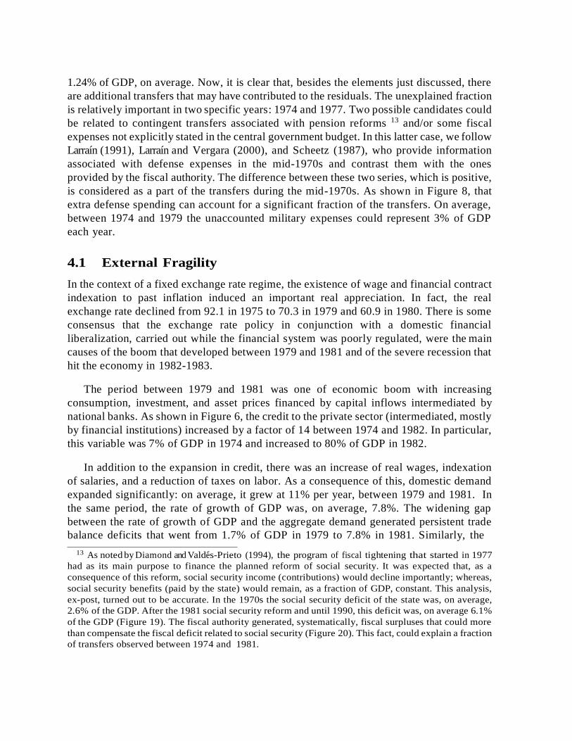
after the 1930s. 2 In terms of fiscal policy, this period was characterized by systematic, and

mild, fiscal deficits as shown in Figure 3. Until 1970, these deficits were relatively small:

on average, 2%. This trend was broken in 1971 and 1972, years in which fiscal deficits

reached 8% and 12% of GDP, respectively. As with inflation, the existence of mild fiscal

deficits was a persistent feature of the Chilean economy, but the figures in 1971 and 1972

were, even for Chilean standards, very high.

The second phase goes from 1974 to 1981 and is characterized by great real and nominal

instability. As shown in Figure 1, there is a pronounced bust-boom cycle in which per capita

GDP declined in 1975 by almost 30%, relative to the predetermined trend. Then it

recovered over a period of five years, so that by 1981 the per capita GDP was almost back

to the trend level. In terms of inflation, this period witnessed the exacerbation of

inflationary pressures of the previous phase. In 1973 inflation reached 400% and in 1974,

after price controls were removed, it reached 600%. This was the highest inflation

1According to World Bank data, per capita GDP in Chile (PPP in constant 2011 US dollars) increased

from US$8.995 in 1990 to US$22.707 in 2016. This is an increase of 153%. In the same period, per

capita GDP in Latin America increased 48%. 2See Velasco (1994).

level ever reached in the history of the country. Inflation declined slowly. By 1981 it had

reached 20% in a context in which the exchange rate was fixed. The fiscal deficit continued

to increase from the previous phase: by 1973 it had reached an unprecedented level of 23%

of GDP. 3 From 1974 onward, there was an important fiscal adjustment. Despite this fact,

inflation remained relatively high until the last years of this phase.

The third phase, from 1982 to 1990, is again a severe bust-boom cycle episode. There

are, however, two features that are different from the previous episode. The first is that the

fiscal discipline, implemented in the mid-1970s, was still present for most of the time. As

shown in Figure 3, in this phase the fiscal deficit was almost zero: 0.1% on average. The

second difference is that inflation increased substantially but did not return to the

hyperinflation levels of the early 1970s. As shown in Figure 2, inflation increased from

10% in 1982 to 27% in 1983. It remained at this level during the whole period. Overall, the

main feature of this phase is the deep and long recession that affected the economy. In

particular, as a result of the severe balance of payment crisis of the early 1980s, real per

capita GDP declined by 20% between 1981 and 1983, as shown in Figure 1. Then, it

gradually recovered, so that in 1990 the per capita GDP was at the same level as in 1981.

The last phase goes from 1991 to 2017. This period marks the beginning of a disinflation

process that was never reverted and that was unprecedented in Chile. It is the longest period

with single-digit inflation rates. As shown in Figure 2, inflation was 22% in 1991, and

declined gradually to 3.5% in 2001. Ten years later, in 2011, inflation was at the same level:

3.3%. By 2017 inflation was 2.2%. In terms of economic growth, this period is

characterized by systematic increases in real per capita GDP each year (two exceptions are

the mild contractions of 1999 and 2009). As shown in Figure 1, per capita GDP almost

doubled between 1991 and 2017. Also, since 1994 this variable has been growing above

the 2% trend. Today real per capita GDP is 24% higher than the level implicit in the

constant trend line. In terms of fiscal behavior, as is clear from Figure 3, the fiscal discipline

of the previous decades was maintained: on average, there was a fiscal surplus of 0.9% of

GDP.

To understand the role of different policies in each of the four phases, we describe the

main macroeconomic developments and discuss the policies implemented and the

limitations, or unexpected consequences, they may have induced. Of course, because of the

length of the paper, not all developments can be described in detail. When appropriate, we

use the contributions in the literature to expalin developments observed in the data. In the

analysis of the different periods, we use the fiscal budget constraint, described in Chapter

2 in this book, as the common conceptual framework. This allows us to associate the

sources and uses of funds and to relate them to economic outcomes, like inflationary

episodes for example.

3The data on public deficits include the deficits of public sector companies.

2 Macroeconomic, debt evolution, and fiscal

adjustment in Chile: 1960-2016

Over the past sixty years Chile experienced radical economic changes and witnessed real

and nominal instability. Policies shifted from an imports substitution strategy, adopted by

many Latin American economies in the 1940s, to market-oriented policies, in which the role

of the state, both as producer and regulator, greatly diminished. In this period Chile

presented a scenario of a wide range of economic policies and economic outcomes. It

experienced almost all definitions of inflation, from moderate to hyperinflation. It had

periods of high fiscal deficits and periods of fiscal surpluses, balance of payments crises,

banking crises, successful and unsuccessful stabilization plans, together with severe

economic recessions in the 1970s and 1980s. In political terms, changes were drastic: after

a relatively long period of democracy since 1925, the military seized power in 1973,

overthrowing Salvador Allende, an elected socialist president. Democracy was recovered

in 1990 and since then seven elected presidents have been in office.

Before discussing in detail the four phases that characterize the Chilean economy, we

present the fiscal budget constraint decomposition in Table 1. It considers, as stressed in

Chapter 2, the sources of fiscal financing: external debt, domestic debt, and seigniorage. It

also takes into account the main fiscal obligations: interest payments and the primary

deficit. Both sources and obligations can change as a consequence of specific policies ;

hence, movements in these variables could reflect ex professo policy innovations. Sources

and obligations, however, may also change as a result of exogenous shocks unrelated to

policy. For instance, a decline in foreign funding could trigger a fiscal adjustment, which is

a response induced by exogenous shocks rather than an explicit fiscal action. Now, we are

able to compute independent measures of all components of the budget constraint. As a

result, total sources and obligations will not necessarily coincide at any point in time.

The difference between the sources and obligations gives rise to the implicit transfer, which

measures the excess or unrecorded spending in any given period (if positive), or they may reflect

unaccounted income sources (taxes) when negative. In Table 1, we present sources, obligations,

and implicit transfers. In general, periods of high volatility are associated with relatively high

and positive implicit transfers. Figure 7 shows the implicit transfer as a percentage of GDP for

every year in the period 1960 to 2016. Implicit transfers increase substantially in the early 1970s

and in the early 1980s. Both were periods of important macroeconomic volatility. In Figure 8

we present all the “off the books” measures that we could identify. As is clear, in different

periods the implicit transfers play a role as an element that put pressure on the public finances.

We can identify the role of public deficits, in the early 1970s, or Treasury notes in the 1980s

issued to rescue the private banks. We will describe in each period the determinants of the

implicit transfers and to what extent they were the source of economic instability or a

consequence of policy responses to attenuate exogenous shocks.

The role of public debt is also crucial to determine the magnitude and sources of implicit

transfers. As seen in Figure 9, public total debt increased substantially in the early 1970s

and early 1980s. This correlation does not necessarily reflect causation, as it may be driven

by exogenous shocks. For instance, the exchange rate depreciation in the mid-1970s

determined an increase in the ratio of external public debt to GDP; however, if we fix the

exchange rate level and generate a counterfactual path for the external debt, Figure 10, we

can see that the increase in the debt position of the government is not only driven by policy

decisions, but also by exogenous shocks. Public debt is also influenced by the implicit

transfers, as these represent a liability; they increase the debtor position of the government.

To illustrate this point, in Figure 11 we present an exercise in which the level of implicit

transfers, denoted τt in Chapter 2, is kept to zero in each period. As is clear, in this

counterfactual scenario the debt position of the government could have been substantially

lower, especially in the 1960s and 1970s.

Now, we describe in more detail the main features that characterize each of the four

phases. The 1960s was a period of relatively high inflation with mild fiscal deficits. The

persistent inflation in the 1960s was, as in the previous periods of Chilean history, closely

related to fiscal deficits and wage indexation. The beginning of the 1970s was a period of

socialist reforms. In this period fiscal deficits increased substantially and were financed by

money issuance. As a consequence, the high inflation episodes of the previous decades

turned to hyperinflation. We think that in this first period, from 1960 to 1973, the main

policy mistake was to rely on inflation taxes to finance an ambitious fiscal policy expansion

that turned out to be unsustainable, because in the end the base over which the inflation tax

was obtained (money) was reduced significantly during hyperinflation periods.

In the mid-1970s, market-oriented reforms were followed and a period of fiscal

adjustment begun. The reduction of inflation was relatively slow in the second half of the

1970s and a stabilization plan, based on fixing the nominal exchange rate, was implemented

in 1978. This policy coincided with the opening of the capital account and the expansion

of the financial sector. Credit was intermediated by private banks to households. Those

credits were, in a large proportion, denominated in foreign currency. Also, they were

provided by foreigners through the local financial system. In this context, there was an

increase in private absorption financed by banks. Eventually, the fixed exchange rate regime

was abandoned and the balance of payments crisis turned into a banking crisis: the private

sector was unable to pay credits denominated in foreign currency once the devaluation

materialized. In this context, the government and the Central Bank intervened in order to

rescue the private sector. We should stress that this crisis was not generated by excessive

fiscal deficits. In fact, the fiscal authority was able, from 1974 until today, to generate mild

fiscal deficits and, in many cases, substantial fiscal surpluses. We think that a crucial policy

mistake in this case was in the sequence of policy reforms. In particular, fixing the

exchange rate, indeed, successfully stabilized inflation. The problem was to fix the

exchange rate at the same time as the economy was completely open to foreign capital

flows intermediated by the financial system.

The policy efforts after the financial crisis were concentrated in putting the country

back on the growth path and fortifying the financial system. The contraction of GDP in

1982 and 1983 was severe, as shown in Figure 1. The main focus of the policies implemented

soon after this recession were designed to solve the balance of payments crisis along with

the financial crisis. To that end, the fiscal authority and the Central Bank designed a

program to rescue the private banks. In this context, the central government implemented

austerity measures with two objectives in mind: to prevent an increase in the fiscal deficit

and to be able to support the rescue plans of the private sector. These austerity measures

were difficult to implement and, of course, were very unpopular. In the end, however, these

painful measures worked. In particular, from 1984 to 1990 the rate of growth in per capita

output was positive and employment recovered. The emphasis on controlling inflation was

diminished and from 1984 to 1990 inflation was much higher than in 1982, when it reached

single-digit values. Despite this fact, inflation was relatively stable and below the

hyperinflation levels of the early 1970s.

In 1990 the per capita GDP was already above, by 12%, the level of 1981. The economy

was growing in a stable way, although inflation problems persisted. The Central Bank was

granted independence in 1989 and, from the early 1990s, it pursued an inflation targeting

regime. This regime was implemented despite the fact that there was, for more of the 1990s,

an exchange rate band. The inflation target was set each year for the year-on-year inflation

of the end of the year (December). The target was slowly declining from 1990 until 1999.

In that year, Chile adopted a flexible exchange rate and a full-fledged inflation targeting

regime was implemented. Specifically, since that year the Central Bank set an inflation

target of 3%, with a tolerance range of 1% (above or below), with the objective of

anchoring market expectations in a two-year horizon. Also, since 1999 the fiscal authority

has followed a structural balance fiscal rule, which despite many changes, is

countercyclical.

Now, there is the view among some economists, Calvo and Mendoza (1998), that the

exchange rate appreciation helped to stabilize inflation during the 1990s. We tend to

disagree with this hypothesis and believe, as shown by Valdes (1998), that the nominal

anchor from 1991 to 1999 was indeed the declining inflation target announced by the

Central Bank. We will provide some evidence of the joint behavior of inflation and exchange

rate that support this hypothesis.

3 Slow growth, public deficits, and inflation: 1960-

1973

In the 1940s Chile, as well as many Latin American economies, adopted an

industrialization process based on import substitution. The idea was to promote the

development of a domestic industrial sector. This, in turn, could be achieved if those

industries were granted a high degree of protection in the form of import tariffs and quotas.

The protection was supposed to be only a temporary measure. Protectionism, however,

became a permanent feature of the Chilean economy. During the 1950s and early 1960s,

this strategy began to run out of steam. 4

During the 1960s, the fiscal authority had access, mainly, to foreign debt, which

increased from 10% of GDP in 1960 to 22% in 1969. Internal public debt, on the other

hand, was at 7% of GDP on average, well below the level it reached in subsequent years

(Figure 9). Inflation was in general high, although below the hyperinflation levels reached

in the mid-1970s (see Figure 4). It moved from 45% in 1963 to 30% in 1969 (see Figure2).

Chile experienced high inflation levels since the 1940s, although during the 1950s this

became a serious problem. In an effort to tackle this problem, in July 1955 the government

hired the Klein-Saks consulting firm to provide technical advice regarding anti-inflationary

policy. The mission’s diagnosis of Chile’s inflationary pressures revolved around four basic

areas: (1) fiscal deficit, (2) monetary expansion, (3) exchange rate policy, and (4) wage rate

policy. In addition, the mission forcefully argued that the state of government finances and,

in particular, the extremely high fiscal deficit was at the heart of the inflationary process

(Edwards, 2007). In this context, when Alessandri was elected in September 1958 an

inflationary stabilization policy was implemented. This consisted of reducing the fiscal

deficit and fixing the nominal exchange rate to the dollar. The fixed exchange rate lasted

until 1962 when a balance of payments crisis took place (this and 1979-1982 are the only

two periods of fixed exchange rates in the whole period of analysis; plus, a short attempt in

1970). During 1959, the first year of Alessandri´s government, the fiscal deficit, that

averaged 2% of the GDP in the previous administration, was drastically reduced and

reverted. In that year the government was able to generate a fiscal surplus of 1.6% of the

GDP. Besides the fiscal adjustment, Alessandri’s administration pushed (and succeeded)

for wage adjustments well below past inflation. In particular, in 1960 wages increased by

10%, despite the fact that past (1959) inflation was 33%. These elements contributed to

anchor inflation expectations and increased the credibility of the stabilization plan. In 1960

and 1961, inflation declined to single digits: 5.5% and 9.6% respectively.

The stabilization plan was apparently a success. The low level of inflation, however,

was not going to last. In 1960 and 1962 the fiscal deficit increased to nearly 3% of GDP.

At the same time a balance of payments crisis took place in 1961 and 1962 inducing the

abandonment of the fixed exchange rate, and the nominal exchange rate depreciated 33%

in October 1962. Soon after the nominal depreciation, prices increased substantially.

Inflation increased to 27.7% in 1962 (mostly explained by events during the last quarter),

45.3% in 1963, and 38.5% in 1964. Hence, inflation returned to its historical levels, with a

fiscal deficit that, though not exorbitant, seemed to constitute a source of inflationary

pressures in a context when fiscal debt was a stable proportion of GDP (around 30%).

4Further details in Edwards and Edwards (1987).

Now, using the budget constraint in Chapter 2, we conclude that financing needs during

Alessandri’s administration were, on average, 2.68% of GDP. In the 1961-1964 period,

primary fiscal deficits constituted the main fiscal obligation. These deficits, representing

3.20% of GDP, were financed mainly by seigniorage (2.21% of GDP) and to a lesser extent

by external debt (0.87% of GDP). Transfers, computed as residual, represented a very small

proportion of overall financing needs: 0.24% of the GDP. As can be seen in Figure 7,

extraordinary transfers (which are calculated as the residual term of budget constraint in

Chapter 2) were close to zero during Alessandri’s administration.

Overall, during Alessandri’s administration, the modest contribution of external and

internal debt to finance the public deficit generated a close link between public deficits,

seigniorage, and inflation. Accordingly, the roots of inflation in that period could be traced

back to persistent fiscal deficits, as was the case in the previous administrations.

Frei was elected with 56% of the votes and took office in November 1964. The

government’s main economic focus was the implementation of basic structural changes,

such as the land reform process and the Chilean participation in the ownership of the Big

Copper Mines. These reforms were slowly implemented in order not to impair

macrostability. There was a certain perception that structural reforms could generate short-

run disequilibriums; hence, when there was an accumulation of inflationary pressures,

priority was to be given to the restoration of macrostability.

Frei’s program was, in terms of social policies, quite ambitious. The public sector was

given a more active role in improving income distribution and increasing the investment

capacity of the economy. Some of the goals of Frei’s program were to increase real wages

in the public sector, government expenditure in social areas (education and health, among

others), and public investment in infrastructure and housing first, and then in other sectors

of the economy. Public investment was expected to be financed b y an increase in income

taxes and more foreign debt.

In macroeconomic terms, Frei’s administration faced significant challenges. One of

them was to stabilize inflation from levels of 40% in 1964. The stabilization plan was to

be gradual: the government expected to bring down inflation to 25%, 15%, and 10% in

each of the first three years in office (Ffrench-Davis 1973). During the first year in office,

1965, inflation declined to 25%, and in 1966 inflation decline further, to 17%. The fiscal

deficit was reduced to 1.5% of GDP in 1966 and continued to adjust in the following years.

This occurred in a context in which GDP growth was, on average, 6% in 1965 and 1966.

The stabilization program was, at least until 1967, successful. There were two elements that

determined that, after 1967, the stabilization plan was no longer viable. First, despite the

fact that the fiscal authority increased its savings (fiscal deficit declined importantly) and

investment, the national level of investment did not increase enough. Second, wages

adjusted much more than was expected initially. During these years, the exchange rate

policy followed was of mini-devaluations to prevent real exchange rate

appreciation. These elements put upward pressure on inflation that began to increase in

1967 (21.9%) until the last year of the government, 1970, to 34.9%.

During Frei’s administration financing sources increased, on average, to 4.52% of GDP.

Compared with the previous government, the availability of foreign debt more than

doubled, representing 2.13% of GDP, the availability of domestic debt followed a similar

increasing pattern. Frei’s administration could not stabilize inflation, particularly at the end

of the government period. On average, inflation was 25%, almost the same figure that

prevailed during Alessandri’s administration (see Figure 2). In this context it is not

surprising that seigniorage under Frei’s and Alessandri’s administrations was nearly

identical: 2.19% of GDP.

In terms of obligations, in this period there was a significant decline in the primary

deficit, which moved from 3.2% of GDP during Alessandri’s administration to 0.90% in

Frei´s administration. This decline in obligations, coupled with a sharp increase in funding

sources, determined an increase in extraordinary transfers, τt, that on average represented

3.99% of GDP. As can be seen in Figure 7, these transfers increased systematically from

1965 to 1970.

Now, in order to identify the nature of the extraordinary transfers, we compute

additional obligations, not accounted in the central government primary deficit, taken

during this administration. As seen in Figure 8, reserve accumulation, expenditures related

to nationalizations, and the financing of public enterprise deficits could explain an

important fraction of the extraordinary transfers, especially at the end of Frei’s

administration. In particular, reserve accumulation represents, on average, 0.8% of GDP in

this period. Nationalizations and the financing of public enterprise deficits represent 0.42%

and 0.53% of GDP, respectively, in the same period.

The beginning of the 1970s was a period of great political instability: three years of a

socialist government ended in 1973 with a military coup that put the armed forces into

power until 1990. Despite the fact that different economic policies were implemented under

each government, some economic problems were long-lasting. This decade witnessed high

inflation, deep contractions in output (1972, 1973, and 1975), and high unemployment. 3.1 The socialist experience: 1970-1973

In September 1970 Allende was elected with 37% of votes and took office in November

1970. His economic program was characterized by several left-wing oriented structural

reforms, including the nationalization of the banking sector and of most industries. In terms

of fiscal policy, an aggressive expansion of government spending generated an

unprecedented increase in the public deficit.

An essential assumption of the economic program was that, in 1970, there was

substantial unutilized capital capacity in the manufacturing sector. In this context, it was

expected that an increase in aggregate demand could be accommodated without generating

inflationary pressures in the short run. As a result, in 1971 an aggressive expansionary fiscal

policy was implemented. The fiscal deficit, as a percentage of GDP, rose from 0.5% in 1970

to 7.3% in 1971; whereas, nominal growth of high-power money increased from 66% in 1970

to 136% in 1971. Not surprisingly, aggregate demand grew at double-digit rates, 10.5% in

1971, while real GDP experienced an expansion of 9.4% with an important decline in the

unemployment rate to 3.9%. In the first year of Allende’s government, prices did not

increase substantially. This fact is attributed to the existence of price controls, and

commodity and factor market rationing. 5

The output expansion of 1971 was not to be sustained in the following years. In 1972

the fiscal deficit increased further, to 11.4% of GDP. The rate of growth of high-powered

money was 178% and prices, despite the official controls, could not be contained: inflation

reached almost 255% on annual basis.6 In terms of real activity, a particularly serious

problem evolved around the de facto process of expropriations of manufacturing firms

implemented by Allende’s administration. In particular, government interventions were

usually preceded by long labor strikes and seizures of the firms’ installations by their

workers that generated significant output losses. In October 1972, a national strike

generated a further decline in activity. 7 In 1972 real output declined by 1.2% and the trade

deficit reached 3.5% of GDP. In 1973 the economic crisis deepened. During this year, the

fiscal deficit almost doubled, reaching 23% of GDP, the highest level experienced in the

previous forty years (see Figure 3). At the same time there were clear signs that the

inflationary process was tending toward hyperinflation. In 1973 inflation reached 433% on

average; whereas, the rate of growth of money was 365% (see Figure 4).

The expansionary policies caused a progressive deterioration of the current account

deficit that was 3% on average in the 1971-1973 period. In this context, the government

used the large foreign reserves it had inherited from the previous administration to finance

those deficits. As a consequence, foreign reserves declined importantly during Allende’s

administration.

From 1971 to 1973 nominal and real volatility increased substantially. Three elements

characterized this period: first, a sequence of increasing fiscal deficits; second, an important

expansion of the high-powered money; and, finally, an inflationary process that became a

hyperinflation. To understand the correlation among the previous variables and fiscal debt

strategies, we follow Sargent (2013) who develops a framework to analyze the inflationary

consequences of government deficits and of alternative ways of financing them. 5More details in Edwards and Edwards (1987) and Corbo and Fischer (1994). 6For the period 1970-1980 we use alternative prices series proposed in Schmidt-Hebbel and Marshall

(1981) due to somewhat unreliable official series. 7Further details in Edwards and Edwards (1987).

To see the extent to which the budget constraint in Chapter 2 can be used to understand

the period of nominal volatility in Chile, we first analyze the relationship between money

and inflation. From November 1970 to April 1972, the annual growth rate of high-powered

money increased from 82% to 108%, without inflation experiencing any substantial change

(see Figure 4). In fact, in April 1972 inflation was 55%, a level higher than the one

experienced the previous decade. 8 In May 1972, however, inflation increased substantially

and, from that date until December 1979, inflation and money growth tended to move

together.

In the absence of enough funding to cover both the fiscal deficit and the interest rate

payments of the debt, the government had to rely on seigniorage as a source of funding (see

Figure 13). As is clear, between 1971 and 1974 the fiscal deficit and seigniorage moved in

the same direction. Furthermore, in quantitative terms, the magnitude of increase is qu ite

similar, with the exception of 1973 in which the fiscal deficit of 22.5% could be highly

financed with seigniorage. The evolution of debt, on the other hand, suggests that Allende’s

government was unwilling (or unable) to increase domestic and foreign borrowing

considerably. On one hand, between 1970 and 1973 foreign public debt was almost

constant at US$ 2 million. This means that, as a percentage of GDP external debt actually

declined in those years (see Figure 9). On the other hand, domestic debt increased, as a

percentage of GDP, from 2.6% in 1970 to 3.2% in 1973 (Figure 12). This increase was, of

course, not enough to finance a fiscal deficit that went, during the same period, from 0.5%

to 22.5% of GDP.

The evidence presented thus far indicates that fiscal deficits, which increased

substantially between 1971 and 1973, could not be completely financed by additional

public debt (domestic and foreign). As a consequence, seigniorage became the most

important source of funds for the fiscal authority. The implication of this strategy was that

inflation became, in the end, a fiscal phenomenon. As shown in Figure 15, the fiscal deficit

was, by far, the most important component of obligations in the 1971-1973 period;

whereas, the sources of funds were seigniorage and, to a smaller degree, an increase in

domestic public debt.

We construct the path of obligations and sources for this period. In the 1971-1973

period financing needs, compared to the 1960s, increased substantially, mainly by the

increased importance of fiscal deficits that averaged 9.10% of GDP. These needs were

covered mostly by seigniorage that represented 12.9% of GDP in that period. The avail-

ability of external funding and domestic funding in US dollars declined greatly during

Allende´s administration. Domestic debt in local currency increased, although it could

finance a small fraction of overall fiscal needs (representing 0.9% of GDP). Transfers, τt

were around 7% of GDP during this period (see Figure 7).

8Price controls and sticky prices may have contributed to a delayed response of prices to the increase

in money growth.

In Figure 8 we present the potential factors behind the residuals of the budget constraint

(i.e., the transfers). We do so by calculating the transfers implied by the budget constraint

considering counterfactual exercises. In these particular years, we can see that the transfers

calculated considering the public enterprise deficits are much lower than the ones without

considering them.9

Thus, during these years, the deficits of public enterprises are the key factor in

explaining the extraordinary transfers. In particular, they represent on average 7.2% of

GDP, which is roughly the same value of transfers in this period. 10

In aggregate terms the 1960-1973 period is characterized by the existence of important

fiscal deficits financed by seigniorage. This is especially true in the 1970-1973 period, so

the average deficit from 1960-1973 of 3.44% of GDP, the seigniorage of 4.43%, and the

implicit transfers of 3.67% in Table 1 underestimate the values observed in Allende´s

government.

4 From stabilization to BOP crisis: 1974-1981

The armed forces, led by General Pinochet, took power in September 1973 after a military

coup overthrew President Allende. Under Pinochet´s administration several structural

changes were carried out. In 1974, Chile followed a stabilization policy based on a

reduction of the government’s deficit (from 22.5% of GDP in 1973 to 0.4% in 1975)

through the elimination of subsidies and the increase in taxes (VAT among others), the

reduction of public employment, and the reprivatization of public companies that were in

a precarious financial situation and required the permanent support of public funds. The

government liberalized prices that were regulated, including a gradual unification of the

multiple exchange rates in place (up to six during Allende´s government). Inflation

continued at high levels; in April 1974 the inflation rate (measured as a year-on-year

variation) increased to more than 700%, reflecting in part the behavior of liberalized

prices.

The monetary base was increased at high but declining rates in the first years of

Pinochet’s government. In 1973, the rate of expansion in nominal terms was 365% while

it was 320%, 283%, and 272% in 1974, 1975, and 1976, respectively. The monetary base

in real terms contracted in 1973 by 34%, while it contracted by 11% in 1974 and 14% in

1975. In 1976 this monetary growth rate in real terms returned to positive values by

increasing 24%. These variations are indicative of a reduction in the real demand of money

until 1976. The monetary base continued increasing in real terms at positive (but lower)

rates until 1981, the year when the financial crisis began.

In 1975, a severe crisis hit the economy, and real output growth declined by 13%. The

recession of 1975 was generated by several factors. First, there was an important decline in

9 In the basic framework, fiscal deficits do not include public enterprises deficits. 10The grey blocks for the years 1971, 1972, and 1973, explain almost all the transfers.

terms of trade at the end of 1974, with copper prices falling by about 50% in real terms and

the price of oil rising by a factor of four. Second, the fiscal adjustment undertaken, which

reduced the fiscal deficit to 0.4% of GDP, had an adverse effect on the aggregate demand

that in 1975 declined by 21%. Inflation did not decline substantially from the previous year:

it was 343% in December 1975. Despite the recession, the reduction of fiscal deficits, the

lower rate of growth of the monetary base, and the openness of the economy, inflation

continued to be high and erratic. This path was incorporated in inflation expectations. The

economy was highly indexed; salaries and the exchange rate were indexed to past inflation. 11This was the case until 1978 when the exchange rate followed a predetermined rate of

devaluation in an effort to anchor inflation expectations and to reduce inflation. This policy

ended with a fixed exchange rate in June 1979. Between 1976 and June 1979 the reduction

in inflation and accumulation of reserves were the driving forces of monetary exchange

rates and financial policies. It is likely that it took longer to reduce inflation because of the

conflicting implications of policies directed at reducing inflation and increasing

international reserves. In 1979 inflation, though not at the level of the early 1970s, was at

double-digit levels, 39% at the end of 1979. Eventually, at the beginning of the 1980s,

inflation was stabilized.

From 1974 to 1976 seigniorage was an important source of revenues, accounting for

7.4% of GDP on average in those years. Those revenue sources were important in a context

in which the burden of foreign public debt increased. In particular, as a result of nominal

exchange rate devaluations12, foreign public debt increased from 27% of GDP in 1973 to

over 40% of GDP in 1975 (Figure 9). To assess the impact of the nominal devaluation on

the public finances, we perform a contrafactual simulation of the foreign public debt. In

particular, we let the nominal rate to devalue, from 1973 onwards, in a way in which the

real exchange rate is constant at its 1973 level. In other words, we generate a counterfactual

nominal exchange rate series that is adjusted by the inflation differential between Chile and

its main trading partners. As shown in Figure 9, nominal devaluations between 1974 and

1975 increased the burden of public external debt by more than 20% of GDP. Nominal

devaluations also increased the burden of domestic debt that, after 1973, was denominated

mainly in US dollars (see Figure 12).

In order to assess the impact of the devaluations on the external fiscal debt, we per-

formed a counterfactual exercise in which we fix the level of the real exchange rate from

1974 onward and compute a counterfactual path for the nominal exchange rate according

to the actual level of foreign prices and domestic inflation. As a result of this exercise, we

obtain a counterfactual path for the evolution of debt. As shown in Figure 10, the

devaluation of the exchange rate contributed to a significant increase in the external debt

position of the fiscal authority.

11See Edwards (1985) and De Gregorio (1991) and Corbo and Fischer (1994) who discuss the importance

of wage indexation as a self-preserving device of inflationary pressures. 12The nominal exchange rate increased from 0.11 in 1973 to 13.05 in 1976.

From 1974 to 1981 the fiscal deficit was reduced substantially (Figure 3). This was

determined by a combination of a sharp increase in fiscal revenues after 1974 (Figure 17)

and an important contraction in government expenditures (Figure 18). In the period 1974-

1981 there was a primary fiscal surplus of 0.6% of GDP. This determined that financial

needs during that period declined importantly from those in the previous administration:

5.0% of GDP (Table 1). In this period the country regained access to foreign financial

markets and, as a consequence, both external debt interest payments (on average 0.8% of

GDP) and external debt (0.3% of GDP) contributed as sources and obligations. In this

period, and particularly between 1974 and 1981, inflation was at high levels and

seigniorage was an important source of financing: 4.5% of GDP. Other sources of financing,

external debt, and domestic debt denominated in US dollars, accounted for nearly 1% of

GDP (Table 1).

The sharp contraction of fiscal deficits in this period along with a positive source of

financing implied that transfers, τt, increased substantially from the previous

administration. In particular, these transfers accounted for nearly 7% of GDP and were

particularly important in 1974 and 1975 (Figure 7). Now, given the fact that the real

exchange rate depreciated substantially in 1974 and 1975, foreign debt could be

contributing to the transfers’ term in the budget constraint. To show the effects that the

depreciations had in the transfers, we compute the contribution of foreign debt assuming

that the nominal exchange rate between 1974 and 1975 evolves so as to keep the real

exchange rate at the same level as the one observed in 1973. In this counterfactual scenario,

transfers in 1974 and 1975 declined importantly. This can be seen in Figure 8 where the

green blocks in the years 1974 and 1975 refer to the transfer, if the real exchange rate would

have been constant.

As discussed above, an objective of the government in the second half of the 1970s was

to increase the level of reserves. Given that increases of the monetary base could be the

consequence of this policy and that it would not have a correlation in the expenditure side

of the budget constraint (thus, affecting the transfers), we compare the increases in reserves

as a share of output with the effective transfers that follow from the equation. As it can be

seen in Figure 8, the direction and size of the increase in reserves seems likely to be an

important factor of the transfers in the years 1976, 1978, 1979, and 1980.

As a summary, we find that from 1974 to 1981 there was an important increase in

seigniorage in a context in which the monetary base was still growing at high rates

(although below the rate of growth reached in 1973). Given that fiscal deficits were

drastically reduced, it follows that implicit transfers during this period were relatively

large: on average nearly 7% of GDP. Now we could identify two elements that could

partially explain those residuals. First, the impact of large depreciations account for, on

average, 1.34% of GDP in that period. Second, reserve accumulation, after the exchange

rate was controlled (in 1978), could also explain an important fraction of transfers:

1.24% of GDP, on average. Now, it is clear that, besides the elements just discussed, there

are additional transfers that may have contributed to the residuals. The unexplained fraction

is relatively important in two specific years: 1974 and 1977. Two possible candidates could

be related to contingent transfers associated with pension reforms 13 and/or some fiscal

expenses not explicitly stated in the central government budget. In this latter case, we follow

Larraín (1991), Larraín and Vergara (2000), and Scheetz (1987), who provide information

associated with defense expenses in the mid-1970s and contrast them with the ones

provided by the fiscal authority. The difference between these two series, which is positive,

is considered as a part of the transfers during the mid-1970s. As shown in Figure 8, that

extra defense spending can account for a significant fraction of the transfers. On average,

between 1974 and 1979 the unaccounted military expenses could represent 3% of GDP

each year.

4.1 External Fragility

In the context of a fixed exchange rate regime, the existence of wage and financial contract

indexation to past inflation induced an important real appreciation. In fact, the real

exchange rate declined from 92.1 in 1975 to 70.3 in 1979 and 60.9 in 1980. There is some

consensus that the exchange rate policy in conjunction with a domestic financial

liberalization, carried out while the financial system was poorly regulated, were the main

causes of the boom that developed between 1979 and 1981 and of the severe recession that

hit the economy in 1982-1983.

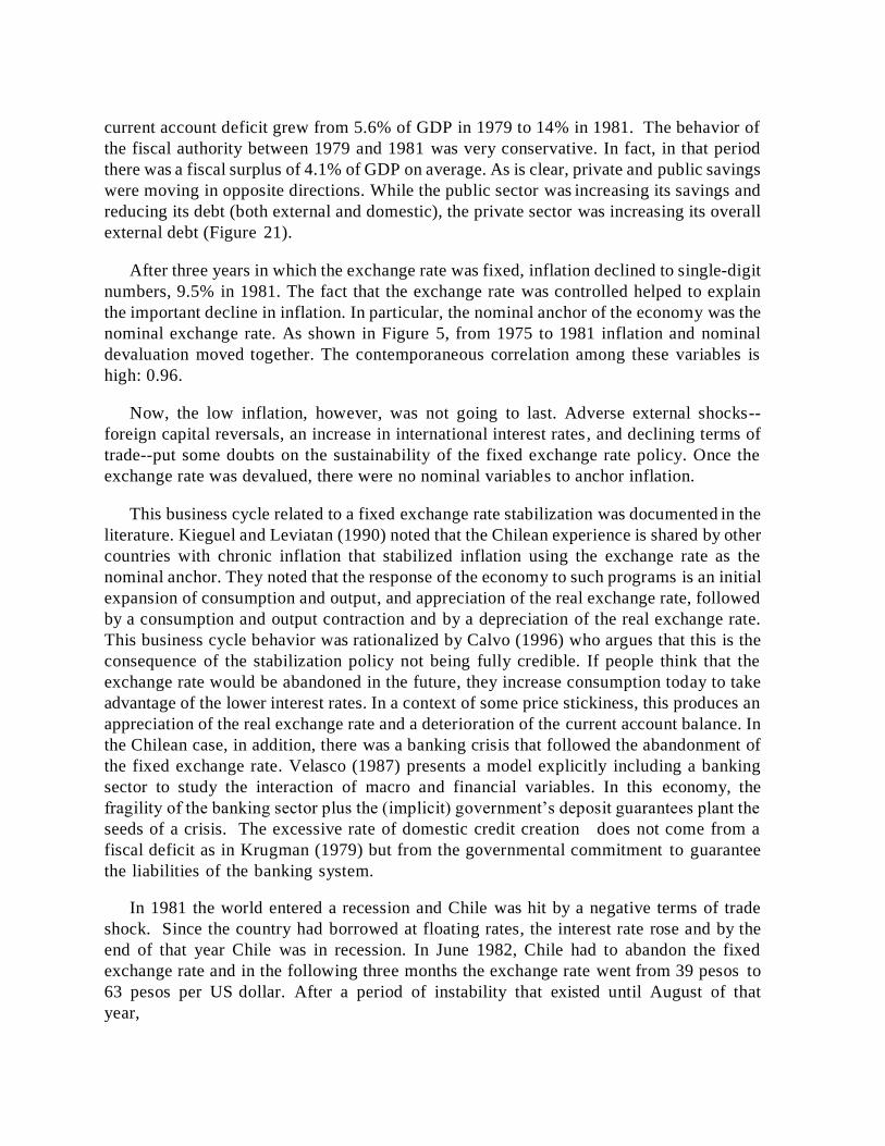
The period between 1979 and 1981 was one of economic boom with increasing

consumption, investment, and asset prices financed by capital inflows intermediated by

national banks. As shown in Figure 6, the credit to the private sector (intermediated, mostly

by financial institutions) increased by a factor of 14 between 1974 and 1982. In particular,

this variable was 7% of GDP in 1974 and increased to 80% of GDP in 1982.

In addition to the expansion in credit, there was an increase of real wages, indexation

of salaries, and a reduction of taxes on labor. As a consequence of this, domestic demand

expanded significantly: on average, it grew at 11% per year, between 1979 and 1981. In

the same period, the rate of growth of GDP was, on average, 7.8%. The widening gap

between the rate of growth of GDP and the aggregate demand generated persistent trade

balance deficits that went from 1.7% of GDP in 1979 to 7.8% in 1981. Similarly, the

13 As noted by Diamond and Valdes-Prieto (1994), the program of fiscal tightening that started in 1977

had as its main purpose to finance the planned reform of social security. It was expected that, as a

consequence of this reform, social security income (contributions) would decline importantly; whereas,

social security benefits (paid by the state) would remain, as a fraction of GDP, constant. This analysis,

ex-post, turned out to be accurate. In the 1970s the social security deficit of the state was, on average,

2.6% of the GDP. After the 1981 social security reform and until 1990, this deficit was, on average 6.1%

of the GDP (Figure 19). The fiscal authority generated, systematically, fiscal surpluses that could more

than compensate the fiscal deficit related to social security (Figure 20). This fact, could explain a fraction

of transfers observed between 1974 and 1981.

current account deficit grew from 5.6% of GDP in 1979 to 14% in 1981. The behavior of

the fiscal authority between 1979 and 1981 was very conservative. In fact, in that period

there was a fiscal surplus of 4.1% of GDP on average. As is clear, private and public savings

were moving in opposite directions. While the public sector was increasing its savings and

reducing its debt (both external and domestic), the private sector was increasing its overall

external debt (Figure 21).

After three years in which the exchange rate was fixed, inflation declined to single-digit

numbers, 9.5% in 1981. The fact that the exchange rate was controlled helped to explain

the important decline in inflation. In particular, the nominal anchor of the economy was the

nominal exchange rate. As shown in Figure 5, from 1975 to 1981 inflation and nominal

devaluation moved together. The contemporaneous correlation among these variables is

high: 0.96.

Now, the low inflation, however, was not going to last. Adverse external shocks--

foreign capital reversals, an increase in international interest rates, and declining terms of

trade--put some doubts on the sustainability of the fixed exchange rate policy. Once the

exchange rate was devalued, there were no nominal variables to anchor inflation.

This business cycle related to a fixed exchange rate stabilization was documented in the

literature. Kieguel and Leviatan (1990) noted that the Chilean experience is shared by other

countries with chronic inflation that stabilized inflation using the exchange rate as the

nominal anchor. They noted that the response of the economy to such programs is an initial

expansion of consumption and output, and appreciation of the real exchange rate, followed

by a consumption and output contraction and by a depreciation of the real exchange rate.

This business cycle behavior was rationalized by Calvo (1996) who argues that this is the

consequence of the stabilization policy not being fully credible. If people think that the

exchange rate would be abandoned in the future, they increase consumption today to take

advantage of the lower interest rates. In a context of some price stickiness, this produces an

appreciation of the real exchange rate and a deterioration of the current account balance. In

the Chilean case, in addition, there was a banking crisis that followed the abandonment of

the fixed exchange rate. Velasco (1987) presents a model explicitly including a banking

sector to study the interaction of macro and financial variables. In this economy, the

fragility of the banking sector plus the (implicit) government’s deposit guarantees plant the

seeds of a crisis. The excessive rate of domestic credit creation does not come from a

fiscal deficit as in Krugman (1979) but from the governmental commitment to guarantee

the liabilities of the banking system.

In 1981 the world entered a recession and Chile was hit by a negative terms of trade

shock. Since the country had borrowed at floating rates, the interest rate rose and by the

end of that year Chile was in recession. In June 1982, Chile had to abandon the fixed

exchange rate and in the following three months the exchange rate went from 39 pesos to

63 pesos per US dollar. After a period of instability that existed until August of that

year,

the exchange rate followed a crawling peg based on a PPP rule, with some discrete and

bigger devaluations (September 1984, 23 %, in February and June 1985, 5% in each case).

The initial devaluation increased the burden of foreign debt deepening the financial cris is.

Jointly with the abandonment of the fixed exchange rate, the compulsory wage indexation

was eliminated. In 1982 the economy experienced a severe recession: output declined by

11% and aggregate demand felt by 19%. Unemployment was nearly 20%, even after

considering the emergency programs established by the government. The monetary base

contracted in real terms by 15% in 1981 and by 41% in 1982 (in both years the nominal

monetary base also diminished). The stabilization plans of the late 1970s had failed.14

5 Saving the banking system: the fiscal burden of the

debt crisis (1982-1990)

The crisis that followed the phase of economic euphoria described above put the banking

system at severe risk. As noted previously, the main debtor with the rest of the world was

the private sector. Between 1975 and 1982 the private foreign debt, as a percentage of GDP,

increased from 10.5% to 41.8%. In the same period, the public external debt declined from

54.3% to less than 27% (see Figure 21). An important part of the private external debt was

intermediated by domestic private banks, and a currency mismatch emerged in their

balance sheets. The sharp depreciation of the peso, in a context of a severe recession, made

many banks insolvent. They could not recover an important proportion of their credits and,

as a consequence, were unable to repay their foreign loans.

In 1982 the Pinochet government approached the IMF in order to obtain financial

assistance to service the foreign debt. Private banks were also approached, and a

rescheduling of the foreign debt was proposed. A standby agreement with the IMF, which

called for a new orthodox stabilization program, was signed. On the other hand, from the

beginning of the debt crisis the government developed a strategy of renegotiating the

foreign debt, but with the declared goal of servicing it in full. The idea was to reestablish

full access to international capital markets. In sharp contrast with other Latin American

countries, default in Chile was never an option. The cost of this strategy was enormous and

was borne by the fiscal authority and the central bank. 15

In order to prevent widespread bankruptcies, the government introduced rescue

programs that were implemented, in an important proportion, by the Central Bank16. As

noted by Sanhueza (2001), the Central Bank undertook three sets of measures to save the

banking system.

14Although 1983 and 1984 the monetary base grew in nominal terms, it continued decreasing in real

terms. It was in 1985 when the monetary base began to grow again in real terms. 15For further discussion, see Edwards (1985) and Corbo and Fischer (1994). 16The Chilean Central Bank has been autonomous since 1989.

First, the Central Bank distributed subsidies to financial institutions in the form of

contracts to buy foreign currency at a price below the market equilibrium (the so-called

Dolar Preferencial program). Until September 1984 this subsidy corresponded to 17% of

debt service and after that month was 35 % until June 1985, when it ended. The losses of

this program incurred by the Central Bank are estimated in US$2.4 billion.

Second, different debt restructuring programs were implemented to alleviate the

situation of debtors. In August 1982, the Central Bank lent US$250 million directly to

debtors to repay their debt with banks. In October of that year, the Central Bank issued

money to buy long-term bonds from the banks, which used these funds to restructure their

debt. In April 1983 and June 1984, two more debt restructure programs were implemented.

These last two programs did not imply an increase in the monetary base because Central

Bank funds given to the banks had to be invested in Central Bank bonds as required by the

targets of the monetary programs agreed upon with the IMF.

Third, several private banks were liquidated and the Central Bank provided the liquidity

necessary to cover bank liabilities and expenses during the liquidation process. For

financial institutions intervened and sold off between 1981 and 1982, the Central Bank

provided special credit lines to pay off liabilities at 100% par value. Between 1982 and

1987, the Central Bank offered to buy part of commercial banks’ and finance companies’

risk portfolio, subject to an eventual buyback. The purpose of this measure was to avoid

the insolvency of banks. The amount of these operations was the equivalent of 30% of the

system’s total outstanding loans for that period, representing 25% of the GDP.

Because of the rescue plan, the Central Bank experienced heavy operational losses. In

1985, as a consequence of having assets with low or zero return and liabilities generating

large payments, the Central Bank experienced an operational loss equivalent to 18% of the

GDP in that year (see Figure 22). The Central Bank was able to access domestic and foreign

financial markets to finance its rescue operations. In practice the Central Bank also relied

on direct transfers from the Treasury in the form of long-term bonds. Those entered the

balance sheet of the Central Bank as assets and appear as domestic fiscal debt. In fact in

1985, the fiscal debt was in a large proportion the Treasury bonds that were transferred to

the Central Bank representing nearly 20% of that year’s GDP (compare Figures 12 and 14)

.

The total net cost to the Central Bank of the portfolio purchase program was equivalent

to 6.7% of the 1983 GDP, when the social cost of capital is used as the discount rate, and

it was equivalent to 5.4% of GDP when the cash flow is measured as a proportion of each

year’s GDP. 17

17This cost is computed by Sanhueza (2001). In this case, cash flow estimates are divided into two parts:

flows from the Central Bank to financial institutions for payment of portfolio purchases, which reached 8.9%

of GDP, and cash flows from financial institutions to the Central Bank for buying back portfolios, which

reached 2.2% of GDP.

The above strategy implied that the rescue plan was mainly financed by issuing domestic

and foreign interest-bearing liabilities of the Central Bank and receiving transfers (long-

term bonds) from the Treasury. For this strategy to be successful and coherent with price

stability, the maturity of the Central Bank debt (and Treasury transfers) have to be such that

it does not put too much pressure on public finances. In the literature there are two,

complementary, ways in which this can be done. First, a long maturity debt contract can

rule out an equilibrium in which default is expected and as a consequence, funds cannot be

raised and default materialized. 18 In the case of Chile, we see in Figures 23 and 24, that

the increase in debt, both by the Central Bank and the fiscal authority was concentrated in

long-term bonds. As a consequence, the long maturity of debt has prevented the existence

of an equilibrium in which deficits are financed by printing money. The same can be said

regarding the public domestic debt. In this case, the bond transferred to the Central Bank

was a twenty-seven-year Treasury bond. Furthermore, this bond was indexed to inflation

and then converted to US dollars in the late 1980s (see Figure 12). As a consequence, debt

repudiation was avoided by having an indexed bond or US dollar-denominated bond. 19

The financial crisis and its implications demanded that the focus of economic policies

were concentrated in the recovery of the economy and of a troubled financial sector.

Regarding the inflation rate, the goal was to maintain it under control but without trying to

reduce it significantly. After 1985 monetary policy involved periodic devaluations in order

to avoid appreciation of the real exchange rate. The result of these policies was an annual

average inflation rate of around 20% between 1982 and 1989. In 1988 elections took place

and the uncertainty about the change in political regime may have affected the higher

inflation rate observed in 1989.

As for the budget constraint accounting used in the paper, during the period from 1982

to 1989, seigniorage reduced its relative importance as a source of financing, representing,

on average, 0.5% of GDP. External debt, on the other hand, had a negative contribution of

1 % of GDP (Table 1). In this period, the main source of financing is related to domestic

credit in local currency (0.2 % of GDP) and domestic credit in US dollars (1.7 % of GDP).

In terms of obligations, the fiscal authority was able to generate a surplus of 1.3% of GDP.

The difference between sources and obligations is such that transfers, τt, represented, on

average, 3.8% of GDP.

Transfers were particularly important in the1982-1989 period (Figure 7). The Treasury

bonds transferred to the Central Bank and the private debt guaranteed account for most of

the transfers in this period (Figure 8). See for example in the year 1985 the transfers are

almost completely explained by the issuance of Treasury notes.

To summarize, in the latter stage of Pinochet’s government, fiscal financing needs were

determined mostly by the fiscal debt the Treasury acquired with the Central Bank.

18See Calvo (1995) and Cole and Kehoe (1996). 19This is stressed by Calvo (1988).

With the exception of the years when the crises were at their peak, fiscal deficits were

absent in this period. In the same way, external debt or domestic (private) debt were not

important sources of funding (Table 1).

6 Fiscal discipline, fiscal rules and inflation targeting:

1991-2017

Chile avoided defaulting its, mainly private, external debt. The cost of this strategy was

assumed by the Central Bank and the fiscal authority (Treasury), which assumed, de facto,

the debt obligations of the private sector. As is clear, the rescue strategy implied an increase

in the debt position of both the Treasury and the Central Bank. To avoid debt dilution and

liquidity problems, debt obligations were indexed and set to long horizons. Now, those

debts have to be, eventually, paid and the only way to achieve this is by generating fiscal

surpluses. This idea, present since the mid-1970s, was followed by the Pinochet

administration in the late 1980s as well as by the democratic governments that came after.

In fact, from 1987 to 2017 the fiscal authority has, in general, generated a surplus (see

Figure 3). Net asset accumulation over time by the central government helped meet future

public-sector commitments that grow at a higher rate than fiscal revenues, and potential

expenditures on contingent liabilities. Furthermore, they also helped financing Central

Bank losses due to the carryover of quasi-fiscal costs of the rescue of commercial banks in

the early 1980s and the sterilization of large capital inflows in the 1990s.

Despite this prudent fiscal policy, and the Central Bank’s autonomy since October 1989,

the reduction of the inflation rate during the 1990s was gradual in order to avoid social

costs of a stabilization plan. It is important to note that this gradual reduction in inflation

rates was possible because of very favorable external conditions and, as discussed above,

the fiscal discipline. Until 1999, there was an exchange rate band. During this period there

was a permanent appreciation pressure on the Chilean peso (it was regularly at the lower

part of the band) because of the significant capital inflows and terms of trade levels. This

implied a lower imported inflation. This crawling peg system was in place until the Asian

crisis. At that moment the pressures on the appreciation of the peso dissipated.

The depreciation of the peso made it difficult to continue defending the band in con-

ditions present after the Asian crisis (decline in terms of trade, tighter credit conditions)

and in September 1999, once uncertainty calmed down, the Central Bank announced the

abandonment of the band and inflation became the only explicit and formal target of the

monetary authority.

There is the view among some economists, Calvo and Mendoza (1998), that the ex-

change rate appreciation helped to stabilize inflation during the 1990s. We tend to disagree

with this hypothesis and believe, as shown by Valdes (1998), that the nominal anchor from

1991 to 1999 was indeed the declining inflation target announced by the Central Bank

during the 1990s. To illustrate this point, it is useful to compare the evolution of the nominal

exchange rate and inflation in the 1990s and in the 1970s. In panel A of Figure 5, we can

see a close correlation between inflation and nominal devaluations from 1975 to 1981. The

sample correlation among those variables is almost one (0.96, to be precise). In panel B

Figure 5 we can see that this correlation is not very strong in the 1991-1999 period. In fact,

the sample correlation is 0.4. In addition, at the end of the sample there is an important and

persistent devaluation without inflationary consequences. In short, the stabilization

experiences of the 1970s and of the 1990s are very different. In the former, the exchange

rate was the facto de nominal anchor of the economy; whereas, in the latter case the nominal

anchor was the inflation target announced by the central bank.

Summing up, fiscal discipline allowed a transition to a smooth road from the troubled

1980s to the adoption of an inflation target regime almost ten years later. This, despite the

fact that the Central Bank was experiencing operational losses (Figure 22) and had a net

worth that has declined steadily since the mid-1980s. In particular, in 2010 the net worth

of the Central Bank was -3.5% of that year GDP (see Figure 25).

An important fiscal institutional arrangement in Chile has been the adoption of a fiscal

rule. In 2001 the government implemented a fiscal policy based on a yearly structural

surplus of 1% of GDP. The basic logic of the rule is to stabilize public expenditures over

the business cycle and the swings of the copper price, preventing excessive adjustments in

periods of recession or unsustainable expenditure levels in periods of prosperity. Hence,

the rule is designed to generate savings in times of prosperity to pay debt contracted in

times of recession, thus softening the economic cycle and granting sustainability to public

finances. At the same time, because it is a known and transparent rule, it reduces uncertainty

for economic agents regarding the future behavior of public finances and stabilizes public

expenditure in economic and socially sensitive areas, such as investment and social

spending. To establish the credibility of this rule, independent panels of experts have a

substantial influence in establishing the reference long-run value of the copper price as well

as the trend growth of GDP.

Going back to our budget constraint framework (in Table 1), from 1991 to 2010 the

fiscal authority has managed to generate surpluses in a systematic way. On average, these

surpluses represented 3% of GDP, relaxing the financing needs of the government. The rest

of the obligations were, on average, a small fraction of GDP. Transfers represented 2.2%

of GDP in the period from 1991 to 2010. As can be seen in Figure 8, fiscal incomes derived

from copper seem to explain an important fraction of the transfers for the years around

2005. A potential additional explanation for these high transfers is that they may constitute

assets accumulated by the state in order to be used when the cycle is adverse or the price

of copper declines. In short, transfers in this period are going to wealth funds20.

20The fiscal responsibility law of 2006 allowed for setting up two sovereign wealth funds and es-

ymt

6.1 Fiscal Rule

The structural balance fiscal rule followed by Chile has experienced several changes over

time, although this has been, in theory, countercyclical 21. In order to determine the de

facto nature of the fiscal rule, we discuss some estimation of the fiscal rule in Chile

performed by Caputo and Irarrazabal (2015). These rules are estimated according to the

specification suggested by Fernandez-Villaverde et al. (2011):

vt = c + αvt−1 + β(ymt − ymt) + γ(τcu,t − τ cu,t) (6.1)

where vt = (gt−τt) , gt is government spending, τt is fiscal income, excluding copper-

related revenues, ym is the real GDP noncopper, and τcu is the fiscal income (in real

terms) related to copper. The bar on top represents the filtered variable (Hodrick-Prescott).

If the fiscal authority is following a countercyclical fiscal rule, the coefficients β and γ are

expected to be negative. The results for the whole sample indicate that fiscal rule has

been countercyclical in the case of noncopper GDP as well as in the case of the price

of copper. From 1990 to 1999, the rule is almost neutral with a long-run response to

the GDP cycle, which is not different from zero, and a response to copper-related

income, which is negative and statistically different from zero. For the latter sample

period, 2000 to 2014, the response to both the GDP cycle and the price of copper increase

(in absolute value) quite importantly. This result suggests that in the last fourteen years

fiscal policy has been decisively countercyclical.

The countercyclical nature of the fiscal rule can explain to some degree the evolution

of transfers since 2000: in times when the GDP cycle and the price of copper cycle are

positive, the fiscal authority generates fiscal surpluses which are, eventually, used to

increase the net asset position of fiscal authority. Hence, it is not surprising that during the

2000s transfers increased importantly and not only explained by higher copper prices.

To summarize, after the debt crisis of the early 1980s it was clear that the only way to

both service the debt and avoid nominal volatility was to generate fiscal surpluses. This

was done in a systematic way since 1987 and, as a consequence, enabled the Treasury to

service its foreign and domestic debt (with the Central Bank). In recent years the fiscal

authority has followed a more countercyclical policy that can explain, to some extent, the

important level that transfers have reached. This, in turn, enabled the Central Bank to

pursue an inflation targeting regime. One important consequence of this strategy is that it

broke the correlation between fiscal deficits, seigniorage, and inflation that was prevalent

in the 1970s (see Figure 13).

tablishing the basic institutional framework necessary for their management. These funds included the

Pension Reserve Fund (PRF), created at the end of 2006, and the Economic and Social Stabilization

Fund (ESSF), launched in early 2007. 21See Tapia (2015), Ffrench-Davis (2016) and Cespedes et al. (2014).

7 Conclusions

In the last fifty years Chile experienced deep structural changes. In the 1960s two different

administrations, Alessandri and Frei, attempted to stabilize inflation. Inflation declined in

some particular years, but it could not be contained permanently. During Alessandri’s

government there was a clear link between inflation and fiscal deficits. This link became

less apparent during Frei’s administration, which adjusted fiscal deficits, but was not able

to reduce inflation. According to our results, in this period seigniorage was used to finance

transfers not explicit in the central government deficits and related to the cost of

nationalizations and the financing of public enterprise deficits.

In the early 1970s a massive increase in government spending, which was not financed

by an increase in taxes or debt, induced nominal instability in the form of high and

unpredictable inflation. Between 1973 and 1974 Chile experienced a hyperinflation process

that had no precedent in the past history. Between 1971 and 1973, seigniorage contributed

to financing the central government deficit. In addition, it contributed to financing the

public enterprise deficits, which represented, on average, 7.2% of GDP in that period.

After the military took power in September 1973, there were some attempts to stabilize

the economy. However, inflation could not be stabilized until the late 1970s. The rate of

growth in high-power money, inflation as well as seigniorage declined, but remained at

relatively high levels. Given that fiscal deficits were drastically reduced, it follows that

implicit transfers during this period were relatively large: on average nearly 7% of GDP.

Reserve accumulations and the impact of large depreciations in the early 1970s can explain

a fraction of these transfers. The rest could be related to contingent liabilities and/or

expenses undertaken by the government and not fully reflected in the fiscal deficit.

In the early 1980s, after the exchange rate was controlled, inflation converged to lower

levels. However, as a consequence of nominal wages that were indexed to past inflation, the

real exchange rate experienced a sharp appreciation. This, in turn, generated external

imbalances that could not be sustained once capital inflows reversed in 1982. In this

context, the exchange rate regime had to be abandoned to restore the external equilibrium.

This, however, came at an important cost: the banking system collapsed and had to be

rescued by the Central Bank and the Treasury. During this period both seigniorage and the

public deficit were very small. The implicit transfers in this period are related to actions

taken by the government and the central bank to safe the private banking sector.

During the 1980s the government did not enter in debt default, but in order to service

its debt, the fiscal authority had to generate, consistently over time, surpluses. Since 1987

this was a systematic policy followed by all administrations. This policy helped achieving

two different, but related, goals. On the one hand, it contributed to reducing the fiscal

debt and, on the other, enabled the Central Bank to pursue an independent monetary

policy aimed at reducing inflation.

In terms of the accounting exercise we implement, we found that there were

unaccounted transfers of 4% of the GDP on average between 1960 to 2010. Once we

include all the potential components associated with the transfers, the residual we obtained

is close to 1% of GDP and it fluctuates in a nonsystematic way.

References

Arenas de Mesa, A., and M. Marcel. 1991. “Reformas a la Seguridad Social en Chile,.” Serie

de Monografías No 5.

Calvo, G. A. 1988. “Servicing the Public Debt: The Role of Expectations .” American

Economic Review 78 (4): 647-61.

_________. 1995. “Varieties of Capital-Market Crises.” Research Department Publications

4008. Inter-American Development Bank, Research Department.

_________, 1996. “Exchange-Rate-Based Stabilisation under Imperfect Credibility.”

Money, Exchange Rates, and Output, chap. 18. Massachusetts Institute of Technology,

365-390.

Calvo, G. A., and E. Mendoza. 1998. “Empirical Puzzles of Chilean Stabilization Policy.”

Technical report.

Caputo, R., and A, Irarrazabal. 2015. “The Business Cycle of a Commodity Exporter.”

Cespedes, L. F., E. Parrado, and A.Velasco. 2014. “Fiscal Rules and the Management of

Natural Resource Revenues: The Case of Chile.” Annual Review of Resource Economics

6 (1): 105-132.

Mimeo.

Cole, H. L., and T. J. Kehoe. 1996. “A Self-Fulfilling Model of Mexico’s 1994-1995 Debt

Crisis.” Journal of International Economics 41 (3-4): 309-330.

Corbo, V., and S. Fischer. 1994. “Lessons from the Chilean Stabilization and Recovery.”

In Bosworth, B. P., R. Dornbusch, and R. Laban, The Chilean Economy: Policy Lessons

and Challenges. Brookings Institution.

De Gregorio, J. 1991. “Indexacion versus Credibilidad en un Programa de Estabilizacion:

La Experiencia Chilena a Mediados de los 70.” Latin American Journal of Economics-

formerly Cuadernos de Economía 28 (83): 189-199.

Diamond, P., and S. Valdes-Prieto. 1994. Social Security Reform. In Bosworth, B. P., R.

Dornbusch, and R. Laban. The Chilean Economy: Policy Lessons and Challenges .

Brookings Institution.

Díaz, J., R. Lu ders, and G. Wagner. 2016. “Chile 1810-2010: La República en Cifras."

Ediciones UC.

Edwards, S. 1985. “Stabilization with Liberalization: An Evaluation of Ten Years of Chile’s

Experiment with Free-Market Policies, 1973-1983.” Economic Development and

Cultural Change 33 (2): 223-54.

_________. 2007. “Establishing credibility: The role of foreign advisors in Chile’s 1955-

1958 stabilization program.” The Decline of Latin American Economies: Growth, Insti-

tutions, and Crises. National Bureau of Economic Research, Inc., 291–332.

Edwards, S., and A. Edwards. 1987. Monetarism and Liberalization: the Chilean Experi-

ment. The University of Chicago Press.

Fernandez-Villaverde, J., P. A. Guerron-Quintana, K. Kuester, and J. Rubio-Ramırez.

2011. “Fiscal Volatility Shocks and Economic Activity.” Technical report. National

Bureau of Economic Research.

Ffrench-Davis, R. 1973. Polıticas Economicas en Chile: 1952-1970.

_________ 2016. “La experiencia de chile con el balance fiscal estructural.” Cuadernos de

Economía 35: 149-171.

Kieguel, M., and N. Leviatan. 1990 “The Business Cycle Associated with Exchange Rate

Based Stabilization.” Unpublished manuscript. Washington, D.C.: The World Bank.

Krugman, P. 1979. “A Model of Balance-of-Payments Crises.” Journal of Money, Credit

and Banking 11 (3): 311-25.

Larraín, F. 1991. “Public Sector Behavior in a Highly Indebted Country: The Contrasting

Chilean Experience. The public Sector and the Latin American Crisis, 89-136.

Larraín, F., and P. Meller. 1991. “The Socialist-Populist Chilean Experience, 1970-1973.”

In Dornbusch, R. and S. Edwards. The Macroeconomics of Populism in Latin America.

National Bureau of Economic Research, Inc., 175-221.

Larraín, F. and R.Vergara. 2000. “Un Cuarto de Siglo de Reformas Fiscales, chapter 3,

pp. In Larraın, F and Vergara, R. La Transformacion Economica de Chile. Centro

de Estudios Publicos, 73-109.

Sanhueza, G. I. 2001. “Chilean Banking Crisis of the 1980s: Solutions and Estimation of

the Costs.” Working Papers Central Bank of Chile 104. Central Bank of Chile.

Scheetz, T. 1987. “Public sector expenditures and financial crisis in Chile.” World Devel-

opment 15 (8): 1053-1075.

Schmidt-Hebbel, K., and P. Marshall. 1981. “Revision del ipc para el perıodo 1970-1980:

Una nota.” Documento del Departamento de Estudios de Empresas BHC .

Tapia, H. 2015. “Fiscal Rule in Chile: From Automatic Pilot to Navigation Device.” Mimeo.

Human Development Report Office.

Valdes, R. 1998. “Efectos de la politica monetaria en chile.” Cuadernos de Economıa

35 (104): 97-125.

Velasco, A. 1987. “Financial Crises and Balance of Payments Crises.” Journal of

Development Economics 27, 263-283.

Velasco, A. 1994. “The state and economic policy: Chile 1952 - 92.” In Bosworth, B. P.,

R. Dornbusch, and R.Laban The Chilean Economy: Policy Lessons and Challenges .

Brookings Institution.

Table 1: Budget Constraint Decomposition: 1960-2016

1960-1973 1974-1981 1982-19990 19991-2016 Periods

Sources:

External debt 0,64% 0,33% -0,99% -0,03%

Domestic debt (CLP + Indexed) 0,23% -0,21% 0,16% 0,60%

Domestic debt (USD) -0,26% 0,36% 1,65% -0,69%

Seigniorage 4,43% 4,53% 0,49% 0,52%

Total 5,04% 5,01% 1,32 % 0,40%

Obligations:

External debt interest payment -0,93% 0,78% 0,63% 0,04%

Domestic debt interest payment (CLP) -0,89% -1,35% -2,14% -0,12%

Domestic debt interest payment (USD) -0,25% -0,53% 0,26% 0,09%

Primary Deficit 3,44% -0,58% -1,28% -2,11%

Parcial Total 1,37% -1,69% -2,52% -2,10%

Implicit Transfers (Residuals) 3,67% 6,70% 3,83% 2,50%

Total 5,04% 5,01% 1,32 % 0,40%

Figure 1: Log of per-capita GDP (1960-2017)

2,50

2,30

2,10

1,90

1,70

1,50

1,30

1,10

0,90

1960 1965 1970 1975 1980 1985 1990 1995 2000 2005 2010 2015

Real per-capita GDP 2% Growth Rate

Source: World Bank and Central Bank of Chile website www.bcentral.cl

27

Figure 2: Inflation in log-scale (1960-2017)

900

90

9

1 1960 1965 1970 1975 1980 1985 1990 1995 2000 2005 2010 2015

Source: Central Bank of Chile.

28

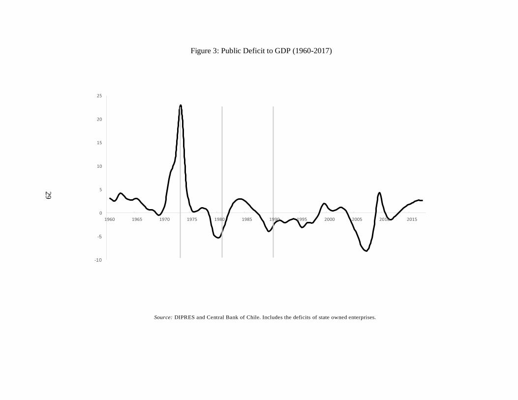
Figure 3: Public Deficit to GDP (1960-2017)

25

20

15

10

5

0

-5

-10

Source: DIPRES and Central Bank of Chile. Includes the deficits of state owned enterprises.

29

Figure 4: High-Powered Money Growth and CPI Inflation (annual rates)

900

800

700

600

500

400

300

200

100

0

1960 1965 1970 1975 1980 1985 1990 1995 2000 2005 2010

SourYcee:ar National Statistics Institute of Chile, Schmidt-Hebbel and Marshall (1981) and Central Bank of Chile website www.bcentral.cl

30

Alessandri Frei Montalva Allende Pinochet I Pinochet II Inflation (YoY)

Money Growth (YoY)

Aylwin Frei Ruiz-Tagle Lagos Bachelet Piñera

%

01-02-75

01-06-75

01-10-75

01-02-76

01-06-76

01-10-76

01-02-77

01-06-77

01-10-77

01-02-78

01-06-78

01-10-78

01-02-79

01-06-79

01-10-79

01-02-80

01-06-80

01-10-80

01-02-81

01-06-81

01-10-81

Fig

ure 5

: S

tab

ilizatio

n P

hase

s: Infla

tion

an

d D

ev

alu

atio

ns

Rate

s

31

600

%

500

%

400

%

300

%

200

%

100

%

0%

27%

22%

17%

12%

7%

2%

-3%

-8%

-13%

So

urce: C

en

tral B

an

k o

f Ch

ile w

ebsite

ww

w.b

cen

tral.c

l

Pan

el A: 1

975 - 1981

(samp

le correlatio

n:0

.96)

Pan

el B: 1

990 - 1999

(samp

le correlatio

n:0

.41)

No

min

al Exchan

ge Ra

te

No

min

al Exchan

ge Ra

te

Inflatio

n

Inflatio

n

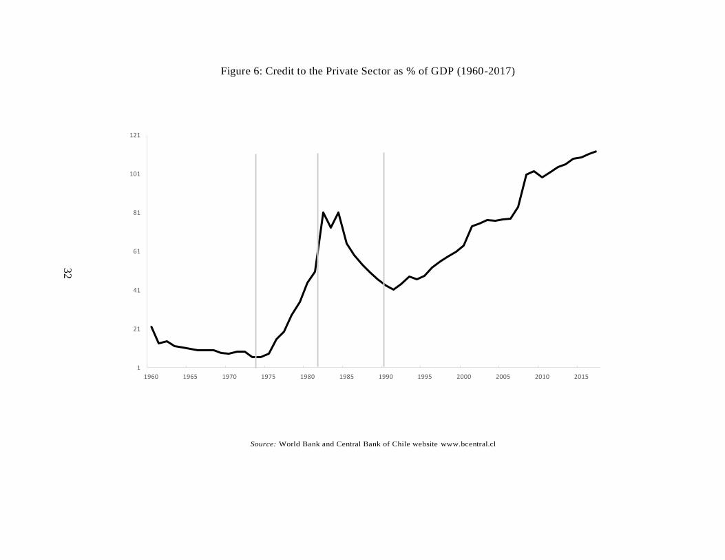
Figure 6: Credit to the Private Sector as % of GDP (1960-2017)

121

101

81

61

41

21

1

1960 1965 1970 1975 1980 1985 1990 1995 2000 2005 2010 2015

Source: World Bank and Central Bank of Chile website www.bcentral.cl

32

Figure 7: Budget Constraint: Baseline Scenario

20%

15%

10%

5%

0%

-5%

-10%

1960 1965 1970 1975 1980 1985 1990 1995 2000 2005 2010 2015 Year

Delta Reserves/GDP Base Residuals Total Residuals

% o

ver

GD

P

33

Figure 8: Potential Factors Behind the Residuals

20%

15%

10%

5%

0%

-5%

-10%

1960 1965 1970 1975 1980 1985 1990 1995 2000 2005 2010 2015 Year

Delta Reserves/GDP Treasury Notes Exchange Rates Private Debt Guarantee Copper Income

Nacionalizations Public Enterprises Deficit Base Residuals Military Total Residuals

% o

ver

GD

P

34

Figure 9: Public Internal and External Debt (as % of GDP)

80

70

60

50

40

30

20

10

0 1960 1970 1980 1990 2000 2010

Source: Central Bank of Chile (2002), “Indicadores EconoYmeiacors y Sociales”; Central Bank of Chile, “Chilean External

Debt” (1977 - 2014); Central Bank of Chile website www.bcentral.cl; General Comptroller Republic of Chile, annual memories and annual Financial Management of the Public Sector Report; General Treasury of the Republic of Chile

Public Internal Debt

Public External Debt (LT)

% o

ve

r G

DP

Figure 10: Long-Term Public External Debt: Counterfactual Evolution w/ Constant Real

Exchange Rate at 1973 (as % of GDP)

80

70

60

50

40

30

20

10

0 1960 1965 1970 1975 1980 1985 1990 1995 2000 2005 2010

Source: Central Bank of Chile (2002), “Indicadores EconYomeaicros y Sociales”; Central Bank of Chile, “Chilean External

Debt” (1977 - 2014); Central Bank of Chile website www.bcentral.cl

Current

Counterfactual

% o

ver

GD

P

Figure 11: Counterfactual Path for Public Debt

Source: Source: author´s calculations.

37

Figure 12: Public Internal Debt (as % of GDP)

60

50

40

30

20

10

Source:

0 1960 1970 1980 1990 2000 2010

Year

General Comptroller Republic of Chile, annual memories and annual Financial Management of the Public Sector Report;

General Treasury of the Republic of Chile; Central Bank of Chile annual memories

38

Indexed

CLP

USD %

ove

r G

DP

30

25 e Lagos Bachelet 2

20

15

10

-5

10

Piñera Bachelet

Total Deficit

Segniorage

Frei Ruiz-Tagl Aylwin Pinochet II Pinochet I Allende

Figure 13: Seigniorage and Public Deficit (as % of GDP)

-

Source:

-15

1960 1970 1980 1990 2000 2010

Year

Díaz, Luders and Wagner (2016) “Chile 1810-2010: La República en Cifras”, Ediciones UC; Central Bank of Chile (2002),

“Indicadores Economicos y Sociales”; “Estado de Operaciones de Gobierno Central Total”, DIPRES; National Statistics Institute of Chile; Schmidt-Hebbel and

Marshall (1981)

% o

ve

r G

DP

39

Figure 14: Public Internal Debt without Treasury Notes (as % of GDP)

60

50

40

30

20

10

Source:

0 1960 1970 1980 1990 2000 2010

Year

Contraloria General de la Republica, annual memories and annual Financial Management of the Public Sector Report;

General Treasury of the Republic of Chile; Central Bank of Chile annual memories

Indexed

CLP

USD %

ove

r G

DP

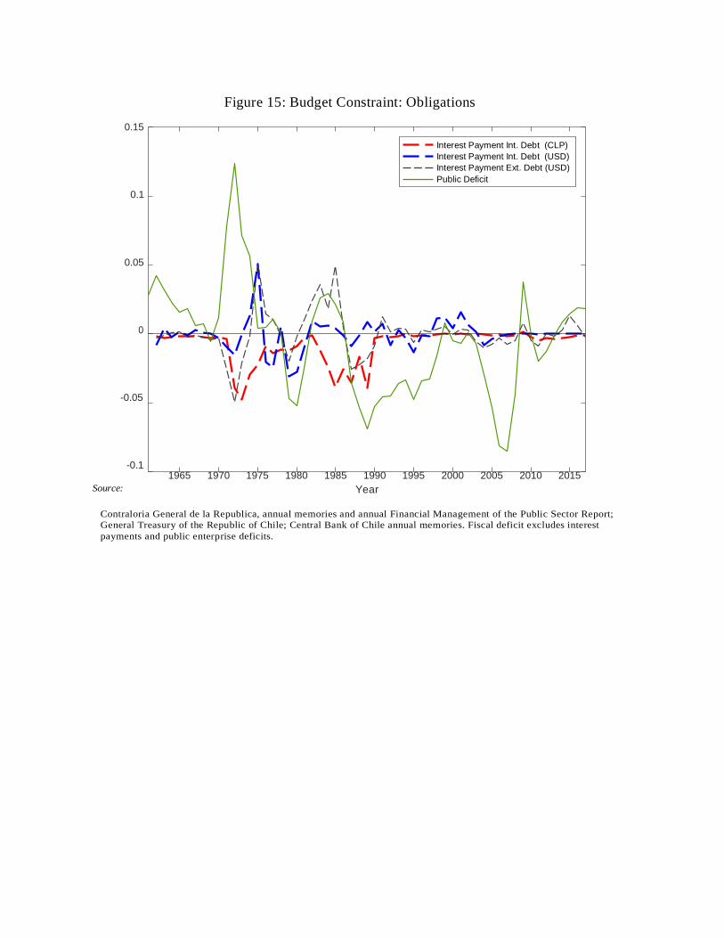
Figure 15: Budget Constraint: Obligations

0.15

0.1

0.05

0

-0.05

Source:

-0.1 1965 1970 1975 1980 1985 1990 1995 2000 2005 2010 2015

Year

Contraloria General de la Republica, annual memories and annual Financial Management of the Public Sector Report;

General Treasury of the Republic of Chile; Central Bank of Chile annual memories. Fiscal deficit excludes interest

payments and public enterprise deficits.

Interest Payment Int. Debt (CLP)

Interest Payment Int. Debt (USD)

Interest Payment Ext. Debt (USD)

Public Deficit

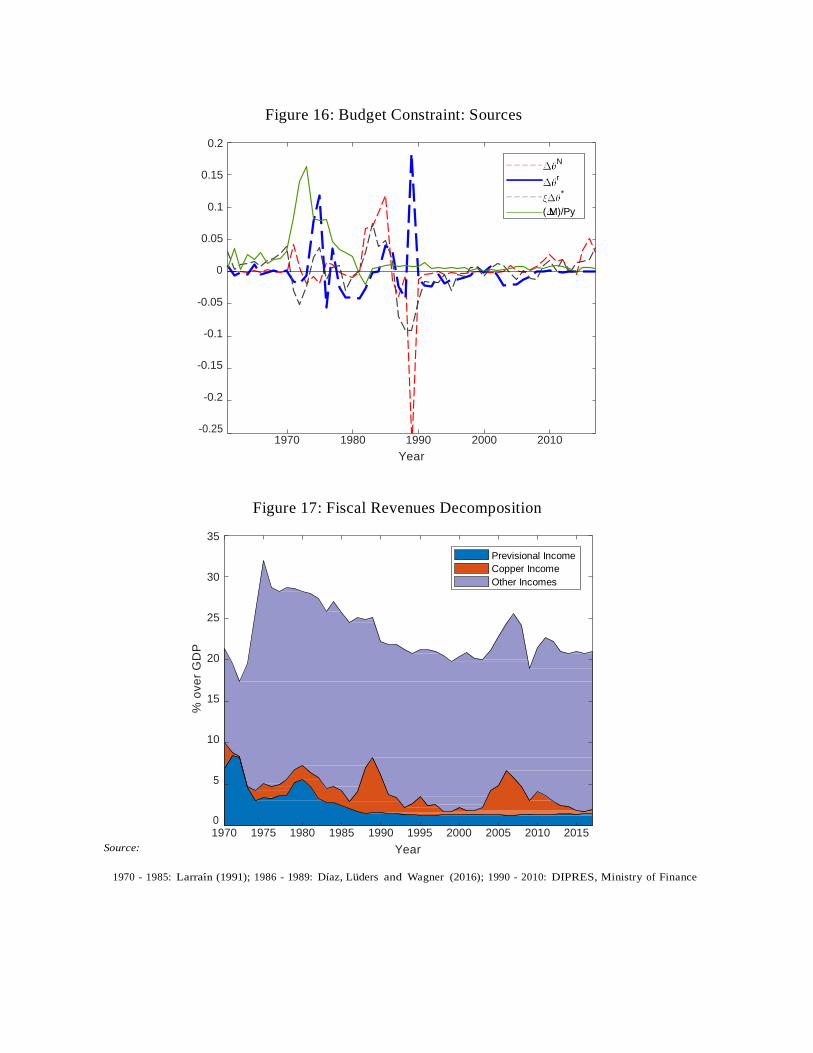
Figure 16: Budget Constraint: Sources

0.2

0.15

0.1

0.05

0

-0.05

-0.1

-0.15

-0.2

-0.25 1970 1980 1990 2000 2010

Year

Figure 17: Fiscal Revenues Decomposition

35

30

25

20

15

10

5

Source:

0 1970 1975 1980 1985 1990 1995 2000 2005 2010 2015

Year

1970 - 1985: Larraın (1991); 1986 - 1989: Díaz, Luders and Wagner (2016); 1990 - 2010: DIPRES, Ministry of Finance

N

r

*

( M)/Py

Previsional Income

Copper Income

Other Incomes

% o

ve

r G

DP

Figure 18: Fiscal Expenditure Decomposition

45

40

35

30

25

20

15

10

5

Source:

0 1970 1975 1980 1985 1990 1995 2000 2005 2010 2015

Year

1970 - 1985: Larraın (1991); 1986 - 1989: Díaz, Luders and Wagner (2016): 1990 - 2010: DIPRES, Ministry of Finance

Figure 19: Social Security Deficit

8

7

6

5

4

3

2

1

Source:

0 1970 1975 1980 1985 1990 1995 2000 2005 2010 2015

Year

1970 - 1985: Larraın (1991); 1986 - 1989: Arenas de Mesa and Marcel (1991); 1990 - 2010: DIPRES, Ministry of Finance.

Previsional Expenditure

Other Expenditures

% o

ve

r G

DP

Reform Social Security Deficit

% o

ve

r G

DP

Figure 20: Fiscal Deficit

25

20

15

10

5

0

-5

-10

Source:

-15 1970 1975 1980 1985 1990 1995 2000 2005 2010 2015

Year

1970 - 1985: Larraın (1991); 1986 - 1989: Arenas de Mesa and Marcel (1991); 1990 - 2010: DIPRES, Ministry of Finance.

Primary Deficit without Social Security Deficit

Primary Deficit

% o

ve

r G

DP

Figure 21: Public (with Central Bank) and Private External Debt (as % of GDP)

90

80

70

60

50

40

30

20

10

Source:

0 1975 1980 1985 1990 1995 2000 2005 2010 2015

Year

Central Bank of Chile (2002), “Indicadores Economicos y Sociales”; Central Bank of Chile, “Chilean External Debt”

(1977 - 2014); Central Bank of Chile website www.bcentral.cl

Public Ext Debt

Private Ext Debt

% o

ve

r G

DP

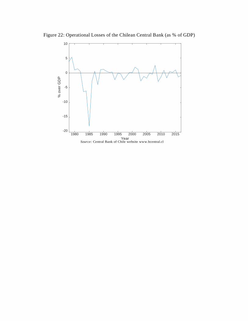
Figure 22: Operational Losses of the Chilean Central Bank (as % of GDP)

10

5

0

-5

-10

-15

-20 1980 1985 1990 1995 2000 2005 2010 2015

Year Source: Central Bank of Chile website www.bcentral.cl

% o

ve

r G

DP

Figure 23: Short and Long Term Public External Debt (as % of GDP)

90

80

70

60

50

40

30

20

10

Source:

0 1975 1980 1985 1990 1995 2000 2005 2010 2015

Year

Central Bank of Chile (2002), “Indicadores Economicos y Sociales”; Central Bank of Chile, “Chilean External Debt”

(1977 - 2014); Central Bank of Chile website www.bcentral.cl

Short Term

Long Term

% o

ve

r G

DP

Figure 24: Short and Long Term Central Bank External Debt (as % of GDP)

30

25

20

15

10

5

Source:

0 1975 1980 1985 1990 1995 2000 2005 2010 2015

Year

Central Bank of Chile (2002), “Indicadores Economicos y Sociales”; Central Bank of Chile, “Chilean External Debt”

(1977 - 2014); Central Bank of Chile website www.bcentral.cl

Short Term

Long Term

% o

ve

r G

DP

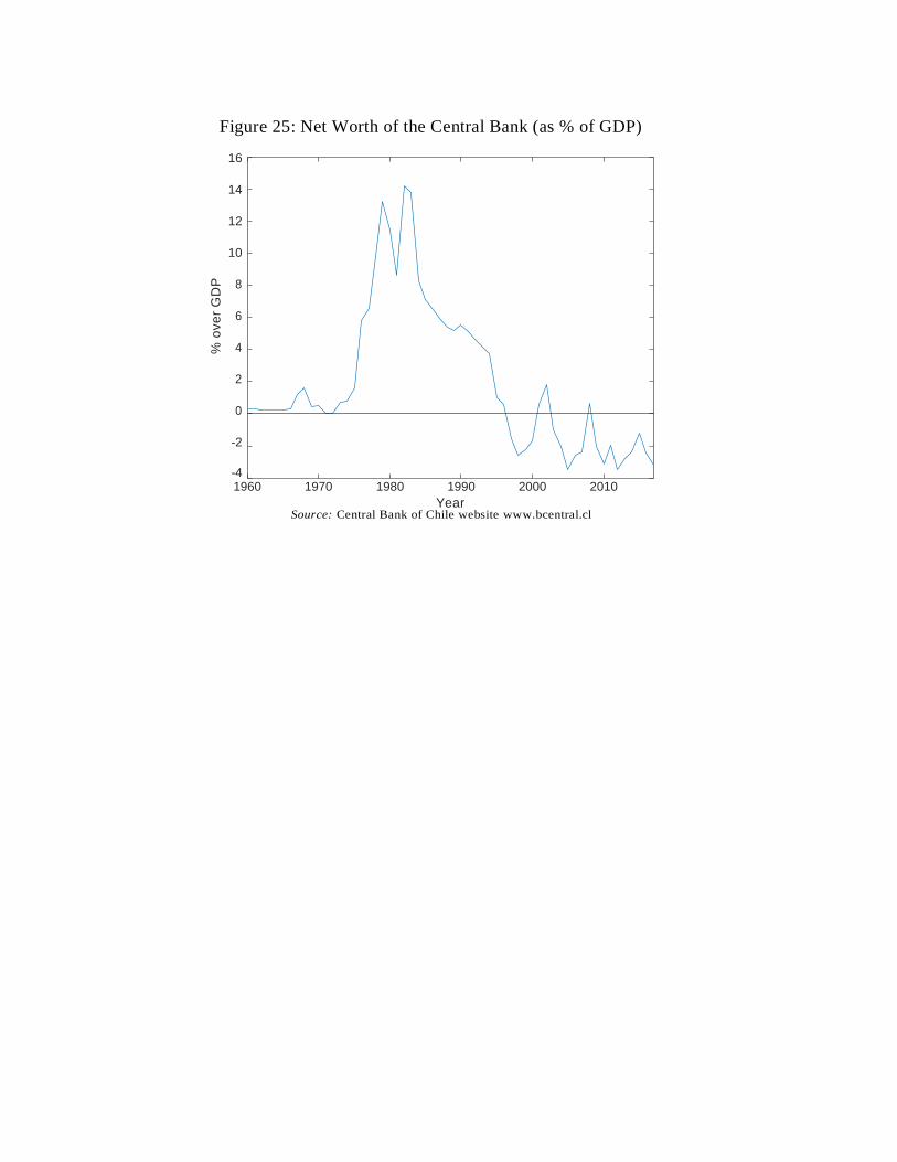
Figure 25: Net Worth of the Central Bank (as % of GDP)

16

14

12

10

8

6

4

2

0

-2

-4 1960 1970 1980 1990 2000 2010

Year Source: Central Bank of Chile website www.bcentral.cl

% o

ve

r G

DP

8