Working Papers in

Trade and Development  

Regional Economic Modelling for

Indonesia of the IRSA-INDONESIA5

Budy P Resosudarmo

Arief A Yusuf

Djoni Hartono

and

Ditya A Nurdianto

December 2009 Working Paper No. 2009/21

 The Arndt‐Corden Division of Economics 

ANU College of Asia and the Pacific 

1 

 

2 

 

Regional Economic Modelling for Indonesia:

Implementation of the IRSA-INDONESIA5

Budy P Resosudarmo The Arndt-Corden Division of Economics

ANU College of Asia and the Pacific The Australian National University

Arief A Yusuf

Padjadjaran University Bandung

Djoni Hartono

University of Indonesia Jakarta

and

Ditya A Nurdianto

The Arndt-Corden Division of Economics ANU College of Asia and the Pacific The Australian National University

 

Corresponding Address : Budy P Resosudarmo

The Arndt-Corden Division of Economics The ANU College of Asia and the Pacific

Coombs Building 9 The Australian National University

Canberra ACT 0200

Email: budy.resosudarmo@anu.edu.au

December 2009 Working paper No. 2009/21

 

3 

This Working Paper series provides a vehicle for preliminary circulation of research results in the fields of economic development and international trade. The series is intended to stimulate discussion and critical comment. Staff and visitors in any part of the Australian National University are encouraged to contribute. To facilitate prompt distribution, papers are screened, but not formally refereed.

 

 

 

 

 

 

 

 

 

 

 

 

 

 

 

 

 

Copies may be obtained from WWW Site http://rspas.anu.edu.au/economics/publications.php

4 

 

 

  

Regional Economic Modelling for Indonesia: Implementation of the IRSA­INDONESIA5  

  

Budy P. Resosudarmo,  Australian National University, Canberra, Australia 

 Arief A. Yusuf,  

Padjadjaran University, Bandung, Indonesia  

Djoni Hartono,  University of Indonesia, Jakarta, Indonesia 

 Ditya A. Nurdianto,  

 Australian National University, Canberra, Australia  

 

 

Abstract: 

Ten years after the implementation of a major decentralization policy, issues of inter‐regional 

disparities in income and rates of natural resource extraction still figure prominently in Indonesian 

economic policy debate.   There is great interest in identifying the macro policies that would reduce 

regional income disparity and better control the rate of natural extraction, while maintaining 

reasonable national economic growth.  In this paper we develop an inter‐regional computable 

general equilibrium model (IRSA‐INDONESIA5) as an appropriate tools for analysis these issues and 

employ it to examine economy‐wide impacts of various policies under consideration. 

JEL: C68, O20, Q50 

Keywords: Computable General Equilibrium, Development Planning and Policy, Environmental Economics. 

 

 

5 

Regional Economic Modelling for Indonesia: Implementation of the IRSA­INDONESIA5  

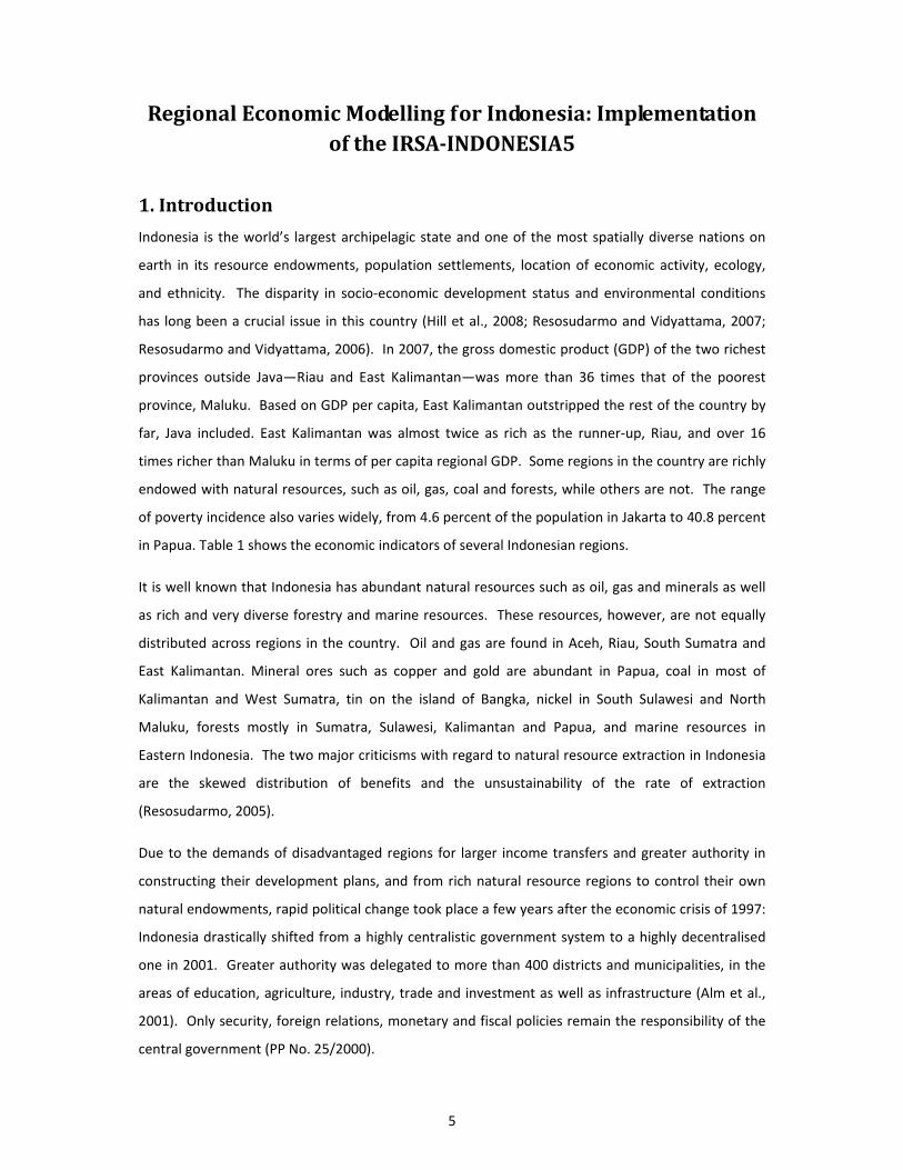
1. Introduction 

Indonesia  is the world’s  largest archipelagic state and one of the most spatially diverse nations on 

earth  in  its  resource endowments, population  settlements,  location of economic activity, ecology, 

and ethnicity.   The disparity  in  socio‐economic development  status and environmental  conditions 

has  long been a crucial  issue  in this country  (Hill et al., 2008; Resosudarmo and Vidyattama, 2007; 

Resosudarmo and Vidyattama, 2006).  In 2007, the gross domestic product (GDP) of the two richest 

provinces outside  Java—Riau  and  East  Kalimantan—was more  than  36  times  that of  the  poorest 

province, Maluku.  Based on GDP per capita, East Kalimantan outstripped the rest of the country by 

far,  Java  included. East Kalimantan was  almost  twice  as  rich  as  the  runner‐up, Riau,  and over 16 

times richer than Maluku in terms of per capita regional GDP.  Some regions in the country are richly 

endowed with natural resources, such as oil, gas, coal and forests, while others are not.  The range 

of poverty incidence also varies widely, from 4.6 percent of the population in Jakarta to 40.8 percent 

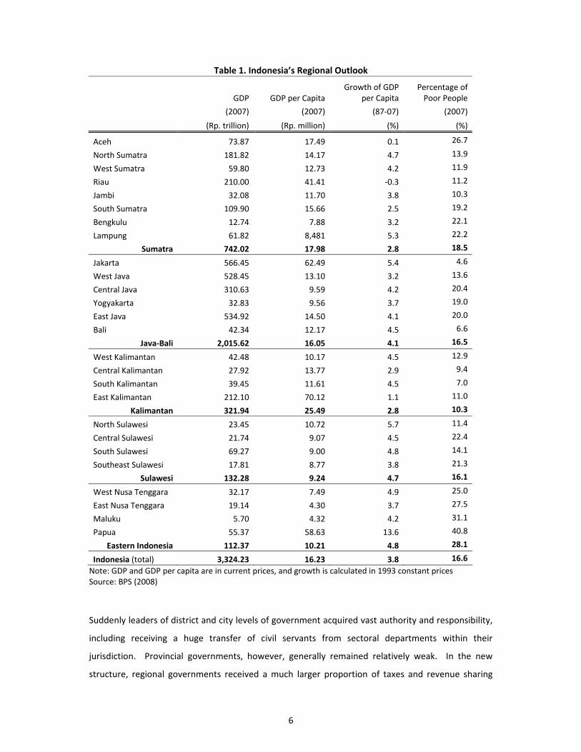
in Papua. Table 1 shows the economic indicators of several Indonesian regions.  

It is well known that Indonesia has abundant natural resources such as oil, gas and minerals as well 

as rich and very diverse forestry and marine resources.   These resources, however, are not equally 

distributed across regions  in the country.   Oil and gas are  found  in Aceh, Riau, South Sumatra and 

East  Kalimantan. Mineral  ores  such  as  copper  and  gold  are  abundant  in  Papua,  coal  in most  of 

Kalimantan  and West  Sumatra,  tin  on  the  island  of  Bangka,  nickel  in  South  Sulawesi  and  North 

Maluku,  forests  mostly  in  Sumatra,  Sulawesi,  Kalimantan  and  Papua,  and  marine  resources  in 

Eastern Indonesia.  The two major criticisms with regard to natural resource extraction in Indonesia 

are  the  skewed  distribution  of  benefits  and  the  unsustainability  of  the  rate  of  extraction 

(Resosudarmo, 2005).  

Due to the demands of disadvantaged regions  for  larger  income transfers and greater authority  in 

constructing  their development plans, and  from rich natural  resource  regions  to control  their own 

natural endowments, rapid political change took place a few years after the economic crisis of 1997: 

Indonesia drastically shifted from a highly centralistic government system to a highly decentralised 

one  in 2001.   Greater authority was delegated to more than 400 districts and municipalities,  in the 

areas of education, agriculture,  industry, trade and  investment as well as  infrastructure (Alm et al., 

2001).  Only security, foreign relations, monetary and fiscal policies remain the responsibility of the 

central government (PP No. 25/2000).   

6 

Table 1. Indonesia’s Regional Outlook 

   GDP  GDP per Capita Growth of GDP 

per Capita Percentage of Poor People 

  (2007)  (2007)  (87‐07)  (2007) 

   (Rp. trillion)  (Rp. million)  (%)  (%) 

Aceh  73.87           17.49  0.1           26.7 

North Sumatra  181.82           14.17  4.7           13.9 

West Sumatra  59.80           12.73  4.2           11.9 

Riau  210.00           41.41  ‐0.3           11.2 

Jambi  32.08           11.70  3.8           10.3 

South Sumatra  109.90           15.66  2.5           19.2 

Bengkulu  12.74             7.88  3.2           22.1 

Lampung  61.82             8,481  5.3           22.2 

Sumatra  742.02           17.98  2.8           18.5 

Jakarta  566.45           62.49  5.4             4.6 

West Java  528.45           13.10  3.2           13.6 

Central Java  310.63             9.59  4.2           20.4 

Yogyakarta  32.83             9.56  3.7           19.0 

East Java  534.92           14.50  4.1           20.0 

Bali  42.34           12.17  4.5             6.6 

Java‐Bali  2,015.62           16.05  4.1           16.5 

West Kalimantan  42.48           10.17  4.5           12.9 

Central Kalimantan  27.92           13.77  2.9             9.4 

South Kalimantan  39.45           11.61  4.5             7.0 

East Kalimantan  212.10           70.12  1.1           11.0 

Kalimantan  321.94           25.49  2.8           10.3 

North Sulawesi  23.45           10.72  5.7           11.4 

Central Sulawesi  21.74             9.07  4.5           22.4 

South Sulawesi  69.27             9.00  4.8           14.1 

Southeast Sulawesi  17.81             8.77  3.8           21.3 

Sulawesi  132.28             9.24  4.7           16.1 

West Nusa Tenggara  32.17             7.49  4.9           25.0 

East Nusa Tenggara  19.14             4.30  3.7           27.5 

Maluku  5.70             4.32  4.2           31.1 

Papua  55.37           58.63  13.6           40.8 

Eastern Indonesia  112.37           10.21  4.8           28.1 

Indonesia (total)  3,324.23  16.23  3.8           16.6 

Note: GDP and GDP per capita are in current prices, and growth is calculated in 1993 constant prices Source: BPS (2008) 

 

Suddenly leaders of district and city levels of government acquired vast authority and responsibility, 

including  receiving  a  huge  transfer  of  civil  servants  from  sectoral  departments  within  their 

jurisdiction.    Provincial  governments,  however,  generally  remained  relatively weak.    In  the  new 

structure,  regional  governments  received  a much  larger proportion of  taxes  and  revenue  sharing 

7 

from natural  extraction  activities  in  their  regions, with  it being  typical  for budgets  to  triple  after 

decentralisation.   Yet  the  issues of  regional  income per  capita disparity and  the excessive  rate of 

natural resource extraction remain (Resosudarmo and Jotzo, 2009).   

There is great interest in identifying the macro policies that would reduce regional income disparity 

and better control  the  rate of natural extraction, while maintaining  reasonable national economic 

growth;  i.e. policies  that will enable  Indonesia  to pursue a path of sustainable development.   The 

question is what kind of economic tool is appropriate to analyse the impact of any macro policy on 

regional and national performances as well as environmental conditions.  This manuscript would like 

to  suggest  that  an  inter‐regional  computable  general  equilibrium  model,  in  particular  IRSA‐

INDONESIA5 which was developed under the Analyzing Path of Sustainable Indonesia (APSI) project, 

is  one  of  the  appropriate  tools  to  analyse  these  issues.    This manuscript  aims  to  explain  IRSA‐

INDONESIA5 and provide several policy analyses using it; in particular, on the issues of development 

gap among regions in the country, achieving low carbon growth and reducing deforestation. 

2. The Computable General Equilibrium Model 

Market equilibrium represents a market condition such that the quantity of goods demanded equals 

the quantity supplied at a price at which suppliers are prepared to sell and consumers to buy.  Thus, 

the current state of exchange between buyers and sellers persists.  When all markets in an economy 

are  in an equilibrium state,  it can be called a general equilibrium condition.   A computable general 

equilibrium (CGE) model uses realistic economic data to model the condition as to how an economy 

reaches  it general equilibrium condition.   CGE then consists of a system of mathematical equations 

representing  all  agents’  behaviour;  i.e.  consumers’  and  producers’  behaviours  and  the  market 

clearing conditions of goods and services in the economy.  This system of equations is usually divided 

into five blocks of equations, namely: 

• The Production Block:  Equations in this block represent the structure of production activities 

and producers’ behaviour. 

• The Consumption Block:   This block  consists of equations  that  represent  the behaviour of 

households and other institutions. 

• The Export‐Import Block:  This block models the country’s decision to export or import goods 

and services. 

8 

• The  Investment  Block:    Equations  in  this  block  simulate  the  decision  to  invest  in  the 

economy,  and  the  demand  for  goods  and  services  used  in  the  construction  of  the  new 

capital. 

• The Market Clearing Block:  Equations in this block determine the market clearing conditions 

for labour, goods, and services in the economy.  The national balance of payments also falls 

within this block. 

An inter‐regional CGE model is a CGE that models multi‐region economies within a country.  In this 

model,  regions  which  consist  of  multiple  sectors  are  typically  inter‐connected  through  trade, 

movements  of  people  and  capital,  and  government  fiscal  transfers.    In  general  there  are  two 

approaches  to  constructing  an  inter‐regional  CGE  model:  the  top‐down  and  the  bottom‐up 

approaches.  The top‐down inter‐regional CGE model solves the general equilibrium condition at the 

national  level, which means  the  optimisation  is  done  at  this  level.  National  results  for  quantity 

variables  are  broken  down  into  regions  using  a  share  parameter.  This  approach,  therefore, 

recognises regional variations in quantity but not in price.   

The bottom–up model on the other hand consists of  independent sub‐regional equilibrium models 

that  are  inter‐linked  and  aggregated  at  the  national  level  as  an  economy‐wide  system.  In  this 

approach, optimisations are done at the regional level. The results of these regional models are then 

combined  to produce  an  aggregate  economy‐wide  outcome.  This  approach,  therefore,  allows  for 

both price and quantity to vary  independently by region. By  implication, this approach enables one 

to analyse the impact of a region specific shock to an economy. The downside, however, is that the 

approach  requires  more  data  and  computing  resources  compared  to  the  top‐down  approach. 

Therefore, sectoral or  regional details often need  to be sacrificed  in order  to compensate  for  this 

drawback.  IRSA‐INDONESIA5 falls into this category of inter‐regional CGE model. 

2.1. CGE on Indonesia 

The CGE model of  the  Indonesian economy became  available  at  the end of  the 1980s.    Included 

among the  first generation of  Indonesian CGEs are  those developed by BPS,  ISS and CWFS  (1986), 

Behrman, Lewis and Lotfi (1988)1, Ezaki (1989), and Thorbecke (1991).  They were developed in close 

collaboration  with  the  Indonesian  National  Planning  and  Development  Agency  (Bappenas),  the 

Ministry of Finance and the Central Statistics Agency (BPS or Badan Pusat Statistik).   They all were 

static  CGE models.    The models  of  Behrman  et  al.  (1988)  and  Ezaki  (1989) were  based  on  the 

Indonesian  input‐output  (IO)  tables, meaning  their  classifications  of  labour  and  household were                                                             1 See Lewis (1991) for detail specification of the CGE utilized. 

9 

limited and their models of household consumption were not complete. The models by BPS, ISS and 

CWFS  (1986) and Thorbecke  (1991) were based on  the  Indonesian  social accounting matrix  (SAM) 

that  is  generally  a more  complete  system  of  data  than  an  input‐output  table.    The models  by 

Behrman et al. (1988) and Thorbecke (1991) were written using GAMS software, while BPS, ISS and 

CWFS  (1986)  and  Ezaki  (1989) were written  in  other  computer  languages.    The models  of  Ezaki 

(1989) and Thorbecke (1991), in addition to the real sector, also include the financial sector in order 

to determine absolute prices endogenously.  All of these CGE models were developed to analyse the 

structural  adjustment program  implemented by  Indonesia  as  a  response  to  the decline  in  the oil 

price in the early 1980s. 

The second generation models of  Indonesian CGEs came out  in  the 2000s.   Among others are  the 

following:    Abimanyu  (2000)  in  collaboration with  the  Centre  of  Policy  Studies  (CPS)  at Monash 

University developed an INDORANI CGE model based on the Indonesian IO table.  It is an application 

of  the  Australian  ORANI model  for  Indonesia  (Dickson,  1982),  and  so works  on  the  platform  of 

GEMPACK Software.   There are two other derivatives of the ORANI model for  Indonesia, which are 

the Wayang model by Warr (2005) and the  Indonesia‐E3 by Yusuf (Yusuf and Resosudarmo, 2008).  

The  advantage  of  Wayang  over  INDORANI  is  that  Wayang  is  based  on  the  Indonesian  social 

accounting  matrix  and  so  has  more  household  classifications.  The  Indonesia‐E3  disaggregated 

households available  in the Indonesian SAM even further  into 100 urban and 100 rural households 

so as to produce gini and poverty indexes.  All of these CGE models are static in nature.  INDORANI 

includes pollution emission equations  for NO2, CO, SO2, SPM and BOD, while  Indonesia‐E3  for CO2 

emissions. 

In  the  GAMS  software  environment,  Azis  (2000)  combined  the  models  by  Lewis  (1991)  and 

Thorbecke  (1991)  to develop a new dynamic  financial CGE model  for  Indonesia and analysed  the 

impact of the 1997–98 Asian financial crisis on the Indonesian economy.  The advantage of this CGE 

is the  inclusion of the  financial sector, so  it can simulate  financial policies.   The  Indonesian Central 

Bank  currently  utilises  this  model  for  their  policy  analysis.    Another  dynamic  CGE  model  for 

Indonesia was developed by Resosudarmo (2002 and 2008).   It doesn’t include the financial sector, 

but does include close‐loop relationships between the economy and air pollutants such as NO2, SO2 

and SPM (2002) and between the economy and pesticide use (2008). 

Concerning inter‐regional models, one of the first such CGEs (IRCGE) for Indonesia was developed by 

Wuryanto  (Resosudarmo et al., 1999).   On  the production  side,  it divides  Indonesia  into  Java and 

non‐Java, while households comprise those  in Sumatra,  Java, Kalimantan, Sulawesi and the rest of 

Indonesia.  It is a static CGE, based on the Indonesian inter‐regional SAM (IRSAM), and runs on GAMS 

10 

platform software.   Another model was developed by Pambudi  (Pambudi and Parewangi, 2004)  in 

collaboration with  the  CPS  at Monash University.  It  is  a  provincial  level  CGE,  static  in  nature,  a 

derivative of  the  inter‐regional version of  the ORANI model, based on  the  Indonesia  IO  table, and 

utilises  GEMPACK  Software.    The models  by Wuryanto  and  Pambudi  are  both  bottom‐up  IRCGE 

models. 

Note  that  there  are  other  CGE models  for  Indonesia  available  of  equal  importance  to  the  ones 

mentioned above.   They have not been mentioned simply because  the authors of  this manuscript 

are not that familiar with them. 

2.2. IRSA­INDONESIA5: Main Features 

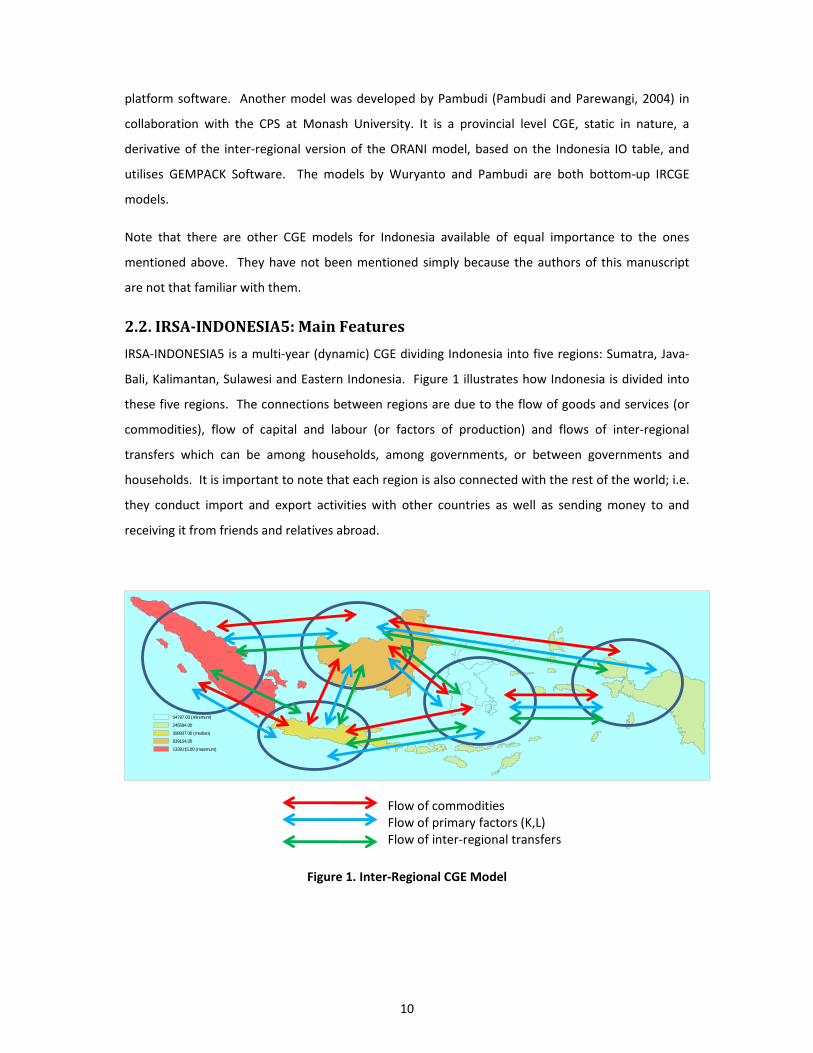
IRSA‐INDONESIA5  is a multi‐year (dynamic) CGE dividing  Indonesia  into five regions: Sumatra, Java‐

Bali, Kalimantan, Sulawesi and Eastern Indonesia.   Figure 1  illustrates how Indonesia  is divided  into 

these five regions.  The connections between regions are due to the flow of goods and services (or 

commodities),  flow  of  capital  and  labour  (or  factors  of  production)  and  flows  of  inter‐regional 

transfers  which  can  be  among  households,  among  governments,  or  between  governments  and 

households.  It is important to note that each region is also connected with the rest of the world; i.e. 

they  conduct  import  and  export  activities with other  countries  as well  as  sending money  to  and 

receiving it from friends and relatives abroad.   

 

Figure 1. Inter‐Regional CGE Model 

 

54797.00 (minimum)

245594.00

398937.00 (median)

639154.00

1339115.00 (maximum)

 

 

 

Flow of commoditiesFlow of primary factors (K,L) Flow of inter‐regional transfers

11 

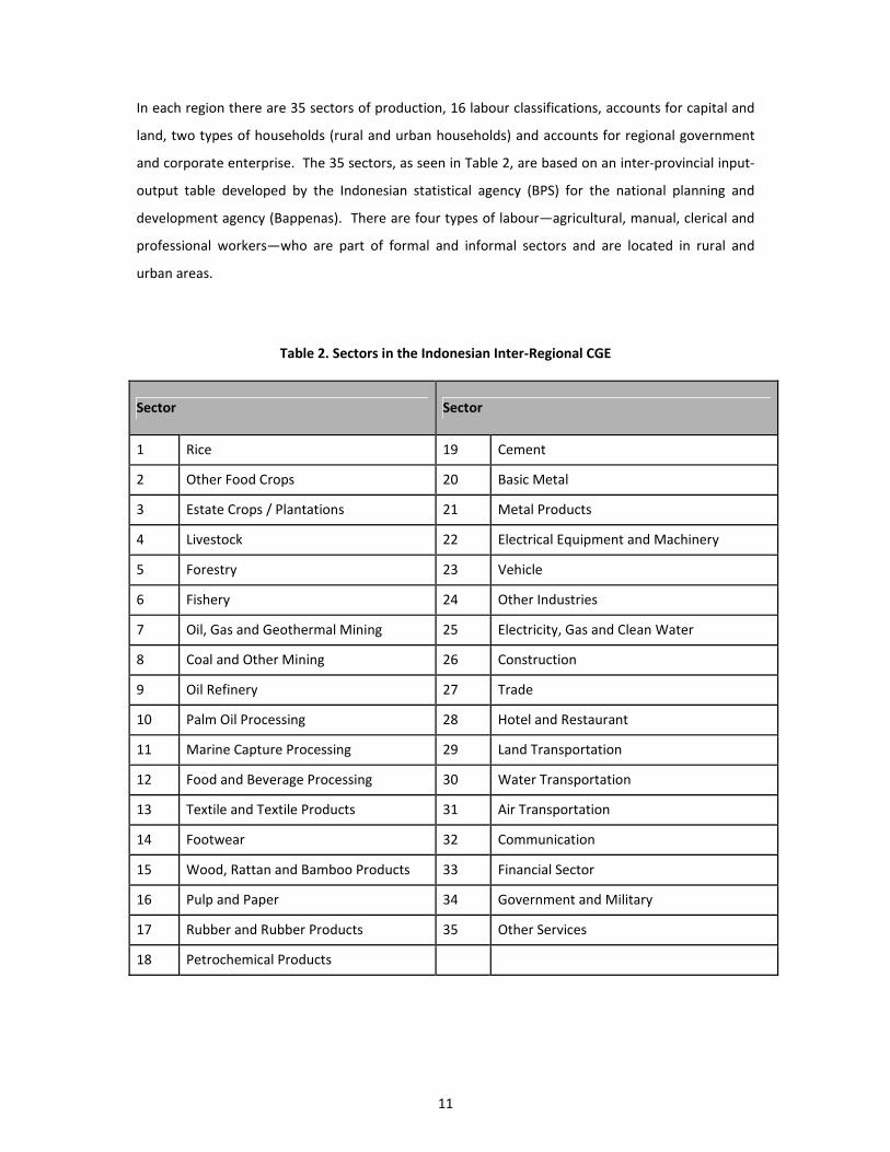
In each region there are 35 sectors of production, 16 labour classifications, accounts for capital and 

land, two types of households (rural and urban households) and accounts for regional government 

and corporate enterprise.  The 35 sectors, as seen in Table 2, are based on an inter‐provincial input‐

output  table  developed  by  the  Indonesian  statistical  agency  (BPS)  for  the  national  planning  and 

development agency (Bappenas).  There are four types of labour—agricultural, manual, clerical and 

professional workers—who  are  part  of  formal  and  informal  sectors  and  are  located  in  rural  and 

urban areas.  

 

Table 2. Sectors in the Indonesian Inter‐Regional CGE 

Sector   Sector  

1   Rice   19   Cement  

2   Other Food Crops   20   Basic Metal  

3   Estate Crops / Plantations   21   Metal Products  

4   Livestock   22   Electrical Equipment and Machinery  

5   Forestry   23   Vehicle  

6   Fishery   24   Other Industries  

7   Oil, Gas and Geothermal Mining   25   Electricity, Gas and Clean Water  

8   Coal and Other Mining   26   Construction  

9   Oil Refinery   27   Trade  

10   Palm Oil Processing   28   Hotel and Restaurant  

11   Marine Capture Processing   29   Land Transportation  

12   Food and Beverage Processing   30   Water Transportation  

13   Textile and Textile Products   31   Air Transportation  

14   Footwear   32   Communication  

15   Wood, Rattan and Bamboo Products   33   Financial Sector  

16   Pulp and Paper   34   Government and Military  

17   Rubber and Rubber Products   35   Other Services  

18   Petrochemical Products          

 

12 

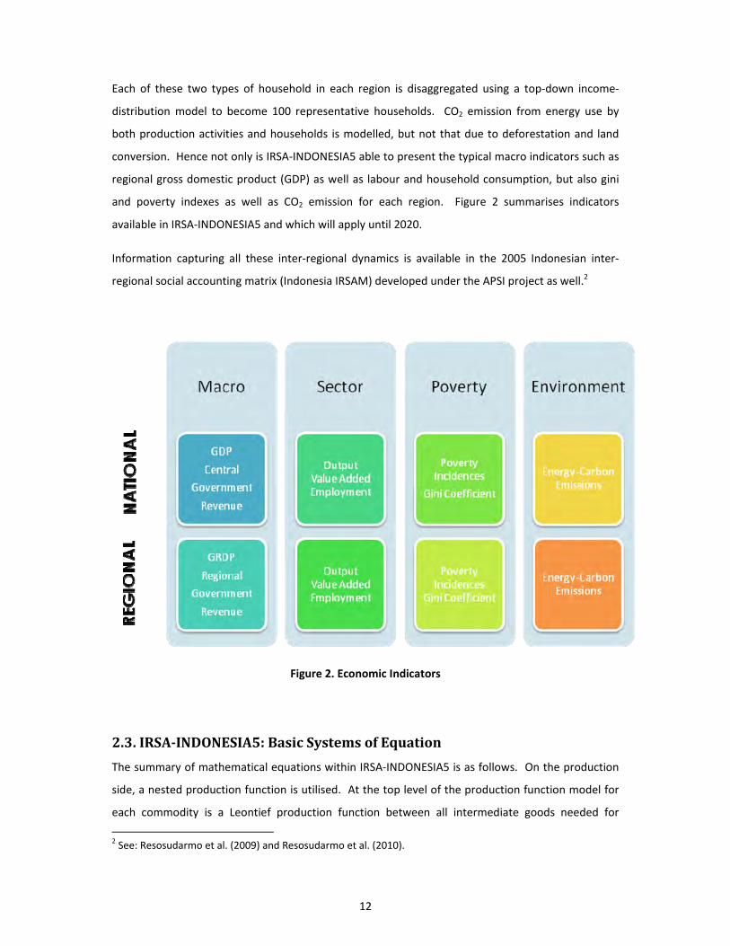
Each of  these  two  types of household  in  each  region  is disaggregated using  a  top‐down  income‐

distribution model  to become 100  representative households.   CO2  emission  from energy use by 

both production activities and households  is modelled, but not that due to deforestation and  land 

conversion.  Hence not only is IRSA‐INDONESIA5 able to present the typical macro indicators such as 

regional gross domestic product (GDP) as well as  labour and household consumption, but also gini 

and  poverty  indexes  as  well  as  CO2  emission  for  each  region.    Figure  2  summarises  indicators 

available in IRSA‐INDONESIA5 and which will apply until 2020. 

Information  capturing  all  these  inter‐regional  dynamics  is  available  in  the  2005  Indonesian  inter‐

regional social accounting matrix (Indonesia IRSAM) developed under the APSI project as well.2 

 

 

Figure 2. Economic Indicators 

 

2.3. IRSA­INDONESIA5: Basic Systems of Equation 

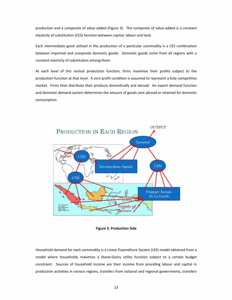
The summary of mathematical equations within IRSA‐INDONESIA5  is as follows.  On the production 

side, a nested production function is utilised.  At the top level of the production function model for 

each  commodity  is  a  Leontief  production  function  between  all  intermediate  goods  needed  for 

                                                            2 See: Resosudarmo et al. (2009) and Resosudarmo et al. (2010). 

13 

production and a composite of value added (Figure 3).  The composite of value‐added is a constant 

elasticity of substitution (CES) function between capital, labour and land.   

Each  intermediate good utilised  in  the production of a particular commodity  is a CES combination 

between  imported and composite domestic goods.   Domestic goods come  from all  regions with a 

constant elasticity of substitution among them. 

At  each  level  of  this  nested  production  function,  firms  maximise  their  profits  subject  to  the 

production function at that level.  A zero profit condition is assumed to represent a fully competitive 

market.  Firms then distribute their products domestically and abroad.  An export demand function 

and domestic demand system determines the amount of goods sent abroad or retained for domestic 

consumption. 

 Figure 3. Production Side 

 

Household demand for each commodity is a Linear Expenditure System (LES) model obtained from a 

model  where  households  maximise  a  Stone‐Geary  utility  function  subject  to  a  certain  budget 

constraint.    Sources  of  household  income  are  their  income  from  providing  labour  and  capital  in 

production activities in various regions, transfers from national and regional governments, transfers 

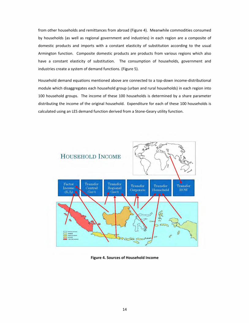
14 

from other households and remittances from abroad (Figure 4).  Meanwhile commodities consumed 

by households  (as well as  regional government and  industries)  in each  region are a  composite of 

domestic  products  and  imports with  a  constant  elasticity  of  substitution  according  to  the  usual 

Armington  function.   Composite domestic products  are products  from  various  regions which  also 

have  a  constant  elasticity  of  substitution.    The  consumption  of  households,  government  and 

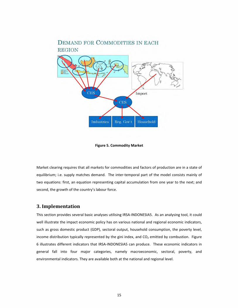
industries create a system of demand functions. (Figure 5).  

Household demand equations mentioned above are connected to a top‐down income‐distributional 

module which disaggregates each household group (urban and rural households) in each region into 

100 household groups.   The  income of  these 100 households  is determined by a share parameter 

distributing the income of the original household.  Expenditure for each of these 100 households  is 

calculated using an LES demand function derived from a Stone‐Geary utility function. 

 

 Figure 4. Sources of Household Income 

15 

 Figure 5. Commodity Market 

 

Market clearing requires that all markets for commodities and factors of production are in a state of 

equilibrium;  i.e. supply matches demand.   The  inter‐temporal part of the model consists mainly of 

two equations: first, an equation representing capital accumulation from one year to the next; and 

second, the growth of the country’s labour force. 

3. Implementation 

This section provides several basic analyses utilising IRSA‐INDONESIA5.  As an analysing tool, it could 

well illustrate the impact economic policy has on various national and regional economic indicators, 

such as gross domestic product  (GDP), sectoral output, household consumption, the poverty  level, 

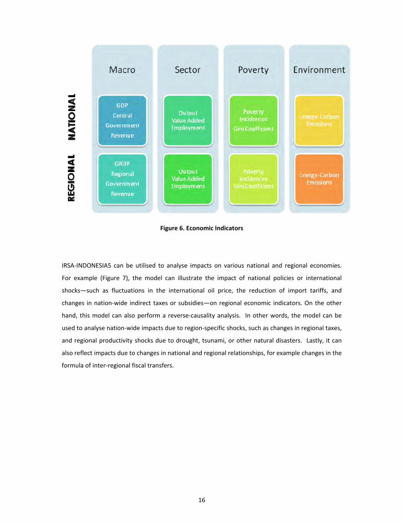
income distribution typically represented by the gini index, and CO2 emitted by combustion.  Figure 

6  illustrates different  indicators that  IRSA‐INDONESIA5 can produce.   These economic  indicators  in 

general  fall  into  four  major  categories,  namely  macroeconomic,  sectoral,  poverty,  and 

environmental indicators. They are available both at the national and regional level.   

 

16 

 

Figure 6. Economic Indicators 

 

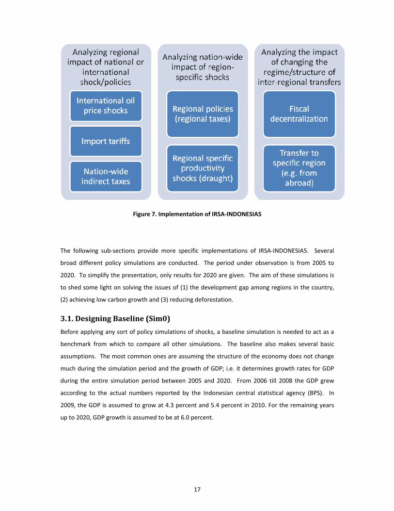
IRSA‐INDONESIA5  can be utilised  to  analyse  impacts on  various national  and  regional economies.  

For  example  (Figure  7),  the model  can  illustrate  the  impact  of  national  policies  or  international 

shocks—such  as  fluctuations  in  the  international  oil  price,  the  reduction  of  import  tariffs,  and 

changes  in nation‐wide  indirect  taxes or subsidies—on  regional economic  indicators. On  the other 

hand,  this model can also perform a  reverse‐causality analysis.    In other words,  the model can be 

used to analyse nation‐wide impacts due to region‐specific shocks, such as changes in regional taxes, 

and regional productivity shocks due to drought, tsunami, or other natural disasters.   Lastly,  it can 

also reflect impacts due to changes in national and regional relationships, for example changes in the 

formula of inter‐regional fiscal transfers.  

 

17 

 

Figure 7. Implementation of IRSA‐INDONESIA5 

 

The  following  sub‐sections  provide more  specific  implementations  of  IRSA‐INDONESIA5.    Several 

broad different policy  simulations  are  conducted.   The period under observation  is  from 2005  to 

2020.  To simplify the presentation, only results for 2020 are given.  The aim of these simulations is 

to shed some  light on solving the  issues of (1) the development gap among regions  in the country, 

(2) achieving low carbon growth and (3) reducing deforestation. 

3.1. Designing Baseline (Sim0) 

Before applying any sort of policy simulations of shocks, a baseline simulation is needed to act as a 

benchmark  from which  to  compare  all  other  simulations.    The  baseline  also makes  several  basic 

assumptions.  The most common ones are assuming the structure of the economy does not change 

much during the simulation period and the growth of GDP;  i.e.  it determines growth rates for GDP 

during  the entire  simulation period between 2005  and 2020.    From 2006  till 2008  the GDP  grew 

according  to  the  actual  numbers  reported  by  the  Indonesian  central  statistical  agency  (BPS).    In 

2009, the GDP  is assumed to grow at 4.3 percent and 5.4 percent  in 2010. For the remaining years 

up to 2020, GDP growth is assumed to be at 6.0 percent. 

18 

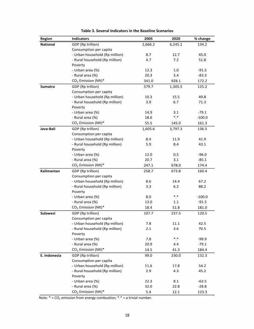
Table 3. Several Indicators in the Baseline Scenarios 

Region Indicators 2005 2020 % change

National GDP (Rp trillion) 2,666.2 6,245.1 134.2

Consumption per capita 

‐ Urban household (Rp million) 8.7 12.7 45.0

‐ Rural household (Rp million) 4.7 7.2 51.8

Poverty

‐ Urban area (%) 12.3 1.0 ‐91.5

‐ Rural area (%) 20.3 3.4 ‐83.3

CO2 Emission (Mt)* 341.0 928.1 172.2

Sumatra GDP (Rp trillion) 579.7 1,305.5 125.2

Consumption per capita 

‐ Urban household (Rp million) 10.3 15.5 49.8

‐ Rural household (Rp million) 3.9 6.7 71.3

Poverty

‐ Urban area (%) 14.9 3.1 ‐79.1

‐ Rural area (%) 18.6 *.* ‐100.0

CO2 Emission (Mt)* 55.5 145.0 161.3

Java‐Bali GDP (Rp trillion) 1,605.6 3,797.3 136.5

Consumption per capita 

‐ Urban household (Rp million) 8.4 11.9 41.9

‐ Rural household (Rp million) 5.9 8.4 43.1

Poverty

‐ Urban area (%) 12.0 0.5 ‐96.0

‐ Rural area (%) 20.7 3.1 ‐85.1

CO2 Emission (Mt)* 247.1 678.0 174.4

Kalimantan GDP (Rp trillion) 258.7 673.8 160.4

Consumption per capita 

‐ Urban household (Rp million) 8.6 14.4 67.2

‐ Rural household (Rp million) 3.3 6.2 88.2

Poverty

‐ Urban area (%) 8.0 *.* ‐100.0

‐ Rural area (%) 13.0 1.1 ‐91.5

CO2 Emission (Mt)* 18.4 51.8 181.0

Sulawesi GDP (Rp trillion) 107.7 237.5 120.5

Consumption per capita 

‐ Urban household (Rp million) 7.8 11.1 42.5

‐ Rural household (Rp million) 2.1 3.6 70.5

Poverty

‐ Urban area (%) 7.8 *.* ‐99.9

‐ Rural area (%) 20.9 4.4 ‐79.1

CO2 Emission (Mt)* 14.5 41.3 184.4

E. Indonesia GDP (Rp trillion) 99.0 230.0 132.3

Consumption per capita 

‐ Urban household (Rp million) 11.6 17.8 54.2

‐ Rural household (Rp million) 2.9 4.3 45.2

Poverty

‐ Urban area (%) 22.3 8.1 ‐63.5

‐ Rural area (%) 32.0 22.8 ‐28.8

CO2 Emission (Mt)* 5.4 12.1 123.3  Note: * = CO2 emission from energy combustion; *.* = a trivial number. 

19 

Table 3 provides several general indicators as a result of this baseline scenario.  It demonstrates the 

Indonesian GDP  in 2020 will be approximately 134 percent higher than  in 2005.  Of the Indonesian 

regions,  it  is expected  that Kalimantan will grow  the  fastest.   Urban poverty at  the national  level 

goes down to 1 percent, while rural poverty is 3 percent in 2020.  The poverty level in rural Sumatra, 

urban  Java, urban Kalimantan and urban Sulawesi  is expected to be zero or close to zero by then.  

The level of total CO2 emission from energy combustion is predicted to be 172 percent higher than in 

2005. 

3.2. Fiscal Decentralisation (Sim1) 

In general, a fiscal decentralisation policy simulation scenario  is where  local governments receive a 

greater  fiscal  transfer allocation  from  the  central government.    In  this  type of policy  scenario  the 

central government is asked to increase its fiscal transfer to local governments through a central‐to‐

regional fiscal transfer, which consists of four types of fund allocation, i.e. tax revenue shared funds, 

natural resource revenue shared funds, specific allocation funds (DAK or Dana Alokasi Khusus), and 

general allocation funds (DAU or Dana Alokasi Umum).  Typically, the central government increases 

its transfers to local governments through the general allocation fund or specific allocation fund. In 

doing so, the central government has at  least three options for allocating the  increased budget for 

each region. The first would be to increase each regional government’s budget proportionally to its 

current  budget;  or  secondly,  it  could  increase  transfers  to  each  regional  government  by  giving 

certain  amounts  of  additional  lump‐sum  funds.  The  implication  is  that  the  central  government 

expenditure will be reduced by an equal amount in both scenarios. 

The hypothesis is that when the central government increases its transfer to regional governments, 

it has to reduce  its expenditure; or  in this simulation, consumption expenditure or expenditure on 

goods  and  services  is  expected  to  decrease.  This  tends  to  have  a  contractionary  effect  on  the 

economy through the decline in demand for commodities. On the other hand, regional governments 

after receiving a  larger fiscal transfer from the central government will  increase their consumption 

expenditure.  This  tends  to  have  an  expansionary  effect  on  the  economy.  Whether  or  not  the 

national demand will decline depends on which  force  is  stronger. The  impact on each  region also 

depends on  the nature of  inter‐regional  trade. The  regions  that  supply a  considerable amount of 

goods and services to the central government will be more affected.  

The third option is that the central government increases its fiscal transfer to some regions, typically 

the  regions  that  lag  behind,  and  decreases  the  amount  of  fiscal  transfer  to  the more  advanced 

regions.  The main hypothesis is that those regions that lag behind will grow faster and so close the 

development  gap  among  regions  in  the  county.    It  is  important  to note  that  the more  advanced 

20 

regions will be negatively affected and so it is not that clear what the impact of this policy will be on 

the national economy. 

The  simulation  run  for  this  manuscript  falls  into  the  third  option;  in  this  simulation,  Eastern 

Indonesia receives an additional transfer of 5 percent from the central government. The additional 

funds for Eastern Indonesia are acquired from an equal amount of fiscal transfer reduction for Java‐

Bali.  The main argument for doing this is that Eastern Indonesia is the least developed region in the 

country and  that  increased  fiscal  transfers  from  the  central government will enable  the  region  to 

catch up. 

3.3. Regional Productivity (Sim2) 

The second simulation deals with regional productivity.   Productivity can arise  from either or both 

capital  and  labour.    Capital  productivity  can  improve  due  to,  among  other  things,  equipment 

maintenance and the adoption of new technology.  Meanwhile, labour productivity can increase due 

to  labour quality  improvements.    These  improvements  could be due  to better  education or new 

knowledge. 

In  this  second  simulation  it  is assumed  that  the  rate of  improvement  in  labour quality  in Eastern 

Indonesia  is higher than the average rate of  improvement  in the other  islands.   Please note that  it 

might be the case that by 2020 the labour quality in Eastern Indonesia will still be lower than in the 

rest of Indonesia.  The main reasons for this faster growth of labour quality in Eastern Indonesia are 

that  it starts from a  lower base, there  is a movement of  labour with higher skills  into the area and 

the quality of education  in  the area  is  improved. Better  labour quality,  in  turn,  translates  into an 

increase in both labour and capital productivity by as much as 1 percent higher than the baseline. 

With  this acceleration of  labour and  capital productivity  it  is expected  that Eastern  Indonesia will 

develop faster than it would under the baseline scenario and this will benefit the nation as a whole 

in terms of poverty reduction and higher growth. 

3.4. Energy Efficiency (Sim3) 

With  increasing  global  concern  regarding  climate  change,  adaptation  and  mitigation  strategies 

become very important.  Indonesia faces a variety of climate change impacts, from sea‐level rise to a 

changing hydrological  cycle and more  frequent droughts and  floods,  to greater  stresses on public 

health.  These will require attention and corrective action if development is to be safeguarded in the 

face of changes  in  the natural world.  Indonesia  itself  is a  significant emitter of greenhouse gases, 

especially  connected  to  deforestation.  However,  reducing  these  emissions  creates  its  own 

challenges; particularly in calculating how these activities will affect the economy and the people.  

21 

The third simulation relates to the improvement in efficiency of energy use.  There are many forms 

energy efficiency can  take, albeit mostly  related  to maintenance and  technological  improvements. 

Energy efficiency can also occur both  in the private and  industrial sectors. Cases where households 

decide to use more energy efficient light bulbs and heaters are an example of how household energy 

efficiency can occur.  Meanwhile, energy efficiency in the industrial sector mainly relates to capital, 

specifically equipment.   Equipment maintenance and technological  improvements are examples of 

how energy efficiency can be achieved in this sector. 

Note  that  the  industrial sector  itself consists of many smaller sectors, such as  food and beverage, 

cement, basic metal, rubber, and others.  As such, energy efficiency in the industrial sector does not 

necessarily  mean  an  increase  in  efficiency  for  all  sectors  at  once.    Implementation  of  IRSA‐

INDONESIA5 can simulate an  increase  in energy efficiency  in all sectors at once or selected sectors 

only.    Furthermore,  in  some  cases,  energy  efficiency  involves  additional  costs,  e.g.  through  the 

adoption  of  new  energy  efficient  technology  acquired  from  abroad  which  the  government  can 

subsidise or, alternately for which the industrial sector bears the entire cost.  

There  is  an  instance  in  the  simulation  run  in  this  manuscript  where  the  stimulus  occurs  from 

equipment maintenance and technological  improvements.   The simulation  looks at the  impact of a 

gradual improvement in energy efficiency of up to 10 percent by 2015 beginning in 2010 in the food 

processing,  textile,  rubber,  cement,  basic metal  and  pulp  and  paper  industries;  i.e.  the  energy 

intensive industries.  

The possible impact will be that these energy intensive industries increase their production since it is 

cheaper for them to produce their products, so enabling them to reduce product prices.  However, 

energy sectors, such as oil and gas, mining and refineries will decline.  The economies of regions that 

rely  most  heavily  on  their  energy  sectors,  particularly  Kalimantan,  will  be  negatively  affected.  

Meanwhile regions where food processing, textile, rubber, cement, basic metal and pulp and paper 

industries are mostly located, particularly Java, will be positively affected. 

3.5. Electricity Sector (Sim4) 

This simulation concerns how electricity has been generated.  It investigates what the impact on the 

economy would be  if  the electricity  sector were  to be more efficient  in utilising energy  inputs  to 

produce  electricity.    First,  electricity  could  be  cheaper  and  so  induce  higher  economic  growth.  

Second,  CO2  emissions  could  be  lower,  in  particular,  since most  coal  is  utilised  by  the  electricity 

power generating sector rather than by other sectors.  

22 

In this simulation, it is assumed that the electricity sector becomes gradually more efficient in using 

fossil  fuels.    It becomes 20 percent more efficient between 2010 and 2015.    It  is assumed  in  this 

simulation that there  is no significant cost associated with the  improvement.    In other words, such 

costs  are  taken  care  of  exogenously.    In  general  this  situation  will  improve  the  economic 

performance of all regions. 

3.6. Energy Subsidy Policy (Sim5) 

Subsidies have  always been  an  important  instrument  for  the  Indonesian  government.    This  issue 

generally relates to the question of who benefits the most from a government subsidy—certainly an 

important issue as it has direct bearing on the purpose of a subsidy.  Of course, there are many types 

of  subsidies,  ranging  from  direct  transfers  to  low‐income  households  from  the  government  to 

industrial subsidies to help reduce production costs in a certain sector.  

This simulation, however, does not look into the impacts of implementing a subsidy.  Instead it looks 

at the  impacts of reducing fuel subsidies.    In other words, the  fifth simulation  looks at the gradual 

elimination of fuel subsidies from the year 2010 until  its full abolition  in 2015.   The entire financial 

gain from subsidy reduction is distributed back into the economy through government spending.  It 

is hard to form expectations on what will happen to the economy.    In general the economy might 

perform better compared to the baseline, but this will probably not be the case in all regions. 

3.7. Carbon Tax (Sim6) 

In this simulation, it is assumed there  is a carbon tax of as much as Rp. 10,000 per ton of CO2 from 

2010  onwards.  This  carbon  tax  revenue  enables  the  government  to  spend more  on  goods  and 

services.  It is expected that industries using highly polluting energy, such as coal, will be negatively 

affected.  On the other hand increasing the government budget will create the stimulus to boost the 

economy.  It remains to be seen which force is stronger.   

3.7. Deforestation (Sim7) 

In this simulation, deforestation outside Java‐Bali is assumed to be reduced by 10 percent from 2012 

onwards mainly due  to effective  control of  logging  activities;  i.e.  the  amount of  logs produced  is 

controlled so as to decline by as much as 10 percent from the amount under the baseline condition.  

Here, no compensation is offered.  In a way, this simulation can also be a benchmark for comparison 

in  other  simulations  related  to  reducing  rate  of  deforestation,  specifically  cases  involving  carbon 

emission reduction compensation.   

The hypothesis is that regions with important forest and forest product industries will be negatively 

affected.  Since these industries are in general situated Indonesia‐wide, including Java where forest 

23 

cover has been limited, all regions will be negatively affected.  This simulation provides an indication 

as to how funding from emission reduction compensation projects such as reducing emission from 

deforestation and forest degradation (REDD) should be channelled. 

4. Observations regarding Results 

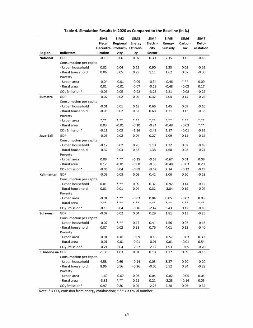
The  following  sections  look  at  the  results  of  simulations mentioned  above.  They  compare  four 

economic  indicators,  namely  gross  domestic  product  (GDP),  household  consumption  per  capita, 

poverty, and carbon emission, for all the simulations with respect to the baseline simulation (Table 

4).    All  numbers  are  percentage  changes;  i.e.  results  from  the  policy  simulations  divided  by  the 

baseline minus one multiplied by a hundred, except for poverty.  Poverty is the difference between 

poverty outcomes from the policy simulation and the baseline situation. 

GDP  is  the most  common measure  of  regional  economic  performance.  A  higher  GDP  tends  to 

indicate  higher welfare  in  the  region.    The  indicator  that most  specifically measures  household 

welfare  is household consumption per capita.   It  is assumed that the more a household consumes, 

the better off  it  is.   This  is the  indicator typically used to differentiate rural and urban households.  

Even when  rural and urban households are affected  similarly, whether positively or negatively,  in 

many cases, magnitudes of the impact do differ.   

Concerning  the poverty  indicator,  the most  common parameter  is  the head‐count poverty  index.  

This index shows the percentage of poor people in a certain region; i.e. those living below a certain 

poverty line.  The World Bank commonly use $1 a day or $2 a day as the poverty line.  BPS produces 

a poverty  line  for each province  in  Indonesia each year.    In 2008, the poverty  line  for urban areas 

was slightly above Rp. 200,000 per capita per month and slightly below Rp. 200,000 per capita per 

month  for  rural areas.   This work will use  the poverty  lines produced by BPS and  so  the poverty 

indicators show the percentage of poor people based on their definitions. 

CO2  emission  indicators  present  the  total  emission  from  fuel  combustion  activities  per  year.    As 

mentioned before, these numbers exclude the amount of emission from deforestation, land use and 

other factors.  

24 

Table 4. Simulation Results in 2020 as Compared to the Baseline (in %) 

SIM1 SIM2 SIM3 SIM4 SIM5 SIM6 SIM7

Region Indicators

Fiscal 

Decentra‐

lization

Regional 

Producti‐

vity 

Energy 

Efficien‐

cy

Electri‐

city 

Sector

Energy 

Subsidy

Carbon 

Tax

Defo‐

restation

National GDP  ‐0.10 0.06 0.07 0.30 2.15 0.15 ‐0.18

Consumption per capita 

‐ Urban household 0.02 0.04 0.21 0.90 1.23 0.05 ‐0.16

‐ Rural household  0.06 0.05 0.29 1.11 1.62 0.07 ‐0.30

Poverty

‐ Urban area ‐0.04 ‐0.01 ‐0.09 ‐0.34 ‐0.46 *.** 0.09

‐ Rural area  0.01 ‐0.01 ‐0.07 ‐0.29 ‐0.48 ‐0.03 0.17

CO2 Emission* ‐0.06 0.05 ‐0.92 ‐3.26 2.21 ‐0.08 ‐0.22

Sumatra GDP  ‐0.07 0.02 0.05 0.32 2.04 0.14 ‐0.26

Consumption per capita 

‐ Urban household ‐0.01 0.01 0.18 0.66 1.45 0.09 ‐0.10

‐ Rural household  ‐0.05 0.02 0.32 0.68 1.71 0.13 ‐0.53

Poverty

‐ Urban area *.** *.** *.** *.** *.** *.** *.**

‐ Rural area  0.03 ‐0.01 ‐0.10 ‐0.24 ‐0.48 ‐0.03 *.**

CO2 Emission* ‐0.11 0.03 ‐1.86 ‐2.48 2.17 ‐0.01 ‐0.35

Java‐Bali GDP  ‐0.03 0.02 0.07 0.27 2.09 0.15 ‐0.15

Consumption per capita 

‐ Urban household ‐0.17 0.02 0.26 1.10 1.22 0.02 ‐0.18

‐ Rural household  ‐0.37 0.03 0.33 1.38 1.68 0.03 ‐0.24

Poverty

‐ Urban area 0.09 *.** ‐0.15 ‐0.59 ‐0.67 0.01 0.09

‐ Rural area  0.12 ‐0.01 ‐0.08 ‐0.36 ‐0.48 ‐0.03 0.20

CO2 Emission* ‐0.06 0.04 ‐0.69 ‐3.57 2.14 ‐0.12 ‐0.19

Kalimantan GDP  ‐0.09 0.03 0.09 0.42 3.06 0.20 ‐0.18

Consumption per capita 

‐ Urban household 0.01 *.** 0.09 0.37 ‐0.92 0.14 ‐0.12

‐ Rural household  0.01 0.01 0.04 0.32 ‐3.84 0.19 ‐0.04

Poverty

‐ Urban area ‐0.01 *.** ‐0.03 0.04 0.05 ‐0.02 0.03

‐ Rural area  *.** *.** *.** *.** *.** *.** *.**

CO2 Emission* ‐0.13 0.04 ‐0.16 ‐2.47 3.43 0.12 ‐0.18

Sulawesi GDP  ‐0.07 0.02 0.04 0.29 1.81 0.13 ‐0.25

Consumption per capita 

‐ Urban household ‐0.07 *.** 0.17 0.41 1.56 0.07 ‐0.15

‐ Rural household  0.07 0.02 0.38 0.76 4.01 0.13 ‐0.40

Poverty

‐ Urban area ‐0.01 ‐0.01 ‐0.09 ‐0.18 ‐0.57 ‐0.03 0.39

‐ Rural area  ‐0.01 ‐0.01 ‐0.01 ‐0.01 ‐0.01 ‐0.01 0.54

CO2 Emission* ‐0.21 0.04 ‐2.57 ‐2.12 1.93 ‐0.05 ‐0.20

E. Indonesia GDP  ‐1.38 1.03 0.01 0.18 1.27 0.09 ‐0.13

Consumption per capita 

‐ Urban household 4.58 0.69 ‐0.14 0.03 3.27 0.20 ‐0.20

‐ Rural household  8.96 0.56 ‐0.26 ‐0.05 5.52 0.34 ‐0.28

Poverty

‐ Urban area ‐1.69 ‐0.07 0.03 0.04 ‐0.82 ‐0.05 0.04

‐ Rural area  ‐3.31 *.** 0.11 0.21 ‐2.23 ‐0.14 0.05

CO2 Emission* 0.97 0.80 0.04 ‐2.23 2.28 0.06 ‐0.32  Note: * = CO2 emission from energy combustion; *.** = a trivial number. 

25 

 

4.1. Fiscal Decentralisation (Sim1) 

Results of this simulation can be seen  in column SIM1 of Table 4.   The  initial  intuition  is that more 

central  government  transfers  to  Eastern  Indonesia  will  benefit  the  region;  i.e.  The  Eastern 

Indonesian  economy  under  this  policy  will  be  higher  than  it  is  under  the  baseline  condition.  

However,  this policy might negatively  affect  the  region,  in  this  case  Java‐Bali, which  receives  less 

fiscal transfer from the central government.  Since the initial condition is that the economy of Java‐

Bali performs better than  that of Eastern  Indonesia, the policy of  increasing  the  fiscal  transfer will 

lower the gap between Eastern Indonesia and Java‐Bali.  

In the short‐run the above intuition might be true, but in the long‐run not.  The lower performance 

of Java‐Bali compared to the baseline situation, in the long‐run negatively affects the performance of 

the whole nation, including Eastern Indonesia.  It can be seen from Table 4 that GDPs of all regions 

decline in 2020.  Even more surprising is that Eastern Indonesia suffers the most in its GDP reduction 

compared  to  the  baseline  even  though  it  receives  an  increase  in  funding  from  the  central 

government.  This shows that Eastern Indonesia does depend on other regions such that an increase 

in revenue to the region cannot compensate for the contraction in all other regions.  

On household consumption per capita, it can be seen that Eastern Indonesia is the only region likely 

to benefit  from  an  increased  transfer of  funding  to  the  region.    The household  consumption per 

capita  in  the  region  increases  by  almost  9  in  percent  urban  areas  and  5  percent  in  rural  areas, 

compared to the situation under baseline conditions.  This higher household consumption per capita 

is translated  into a  lower  level of poverty by as much as 3 and 2 percent  in urban and rural areas, 

respectively. 

Household consumption per capita does not change much in other regions.  In this simulation Java‐

Bali  faces  a  lower  transfer  of  funding  from  the  central  government  compared  to  the  baseline 

situation, and so  it  is natural  that household consumption per capita  in  this  region  is affected  the 

most negatively.   A  lower household consumption per capita  is then translated to a higher poverty 

level in this region.  Observing what is happening in the Eastern Indonesian and Java‐Bali regions, it 

can be concluded that shifting funding from rich to poor regions does work in reducing the poverty 

level of poor regions. 

4.2. Regional Productivity (Sim2) 

In this scenario, productivity  in Eastern  Indonesia alone  improves  faster and  induces a higher GDP 

for  Eastern  Indonesia  in 2020  than  it does under  the baseline  condition. Better productivity  also 

26 

induces a higher consumption per capita  in rural and urban areas  in these regions, and translating 

into a lower level of poverty.  In rural areas, however, the change in the poverty level is minimal. 

The other regions also benefit from a more productive Eastern Indonesia as their GDPs  in 2020 are 

also  slightly higher  in  this scenario compared  to  the baseline.   Nevertheless  the  impacts on other 

regions’ GDPs are not that large and so household consumption per capita in other regions are only 

marginally higher than the baseline situation.  Poverty levels in rural and urban Sulawesi, rural Java‐

Bali and rural Sumatra in 2020 are lower than their baseline levels. 

It can be  seen  in  this  scenario  that productivity  improvement achieves both  the  targets of higher 

national  economic  growth  and  reduction  in  the  development  gap  between  regions.    Given  this 

result, there is certainly room for the government to incur “extra” costs to ensure the improvement 

of productivity such as by improving the educational system in less developed regions. 

4.3. Energy Efficiency (Sim3) 

More efficient use of energy  in  the energy  intensive sectors—i.e.  food processing,  textile,  rubber, 

cement,  basic metal  and  pulp  and  paper  industries—is  expected  to  lower  the  operation  costs  of 

those sectors, and enable them to sell their products at a lower price.  This generates higher demand 

for the products of those sectors and so induces higher returns to factor inputs including incomes of 

workers  who  work  in  those  sectors.    These  higher  returns  potentially  improve  household 

consumption  so  households will  be  able  to  spend more, with  the  outcome  that  the  economy  is 

expected  to grow.   On  the other hand, more efficient use of energy  reduces demand  for energy 

products meaning  lower  returns  to  factor  inputs  in  the  energy  sectors  including  work  income.  

Ultimately,  these  lower  incomes  could  potentially  reduce  the  economy.    Hence, more  efficient 

energy usage could either lower or raise the economy. 

The result in column SIM3 in Table 4 shows that more efficient energy usage by the energy intensive 

sector does induce a higher GDP in 2020 compared to the baseline scenario.  It is important to note 

that in those regions where energy sectors dominate, regional GDPs in the short run might be lower 

than under  the baseline  scenarios.   However, since other  regions grew  faster,  in  the  long‐run  the 

regions where energy sectors are dominant will  receive  spillover benefits.    It  turns out under  this 

scenario such benefits  in  the  long‐run are higher  than  the negative  impact of a  lower demand  for 

energy in the short‐run. 

In  this  scenario, household  consumption per  capita  in  general  is higher  in  all  regions  than  in  the 

baseline scenario.   This higher  income per capita  is translated  into a  lower  level of poverty  in most 

27 

regions, except for urban Sumatra and rural Kalimantan.  In those areas, the levels of poverty remain 

the same as under the baseline condition.  

Under  this  scenario  CO2  emission  from  energy  combustion  in  2020  is  lower  than  in  the  baseline 

condition, representing  lower consumption of fuels.   The ability to improve energy efficiency in the 

energy intensive sectors not only creates higher growth, but also reduces CO2 emission from energy 

combustion.   Therefore  the ability  to  improve energy efficiency  in  the energy  intensive  sectors  is 

certainly  one  way  to  control  CO2  emission.    Since  the  economy  would  benefit  from  this 

improvement,  there  is  room  for  the  government  to  create programs or  incentives  to  ensure  this 

improvement in energy efficiency. 

4.4. Electricity Sector (Sim4) 

A more  efficient  electricity  sector makes  it  cheaper  to  produce  electricity.    The  lower  price  of 

electricity lowers costs in all other sectors except for the primary energy sector.  Households will also 

be able to consume more goods and services other than electricity.  The overall potential  impact is 

the  economy  becoming  larger  than  the  baseline  situation.    On  the  other  hand,  due  to  a more 

efficient electricity sector, primary energy sectors might decline and so potentially negatively affect 

the economy.   Ultimately  it  remains  to be  seen whether or not a more efficient electricity  sector 

benefits the economy. 

Column SIM4  in Table 4 shows that  it turns out that a more efficient electricity sector does  induce 

higher GDPs in all regions by 2020 compared to the baseline situation. The benefits of having a more 

efficient electricity  sector are greater  than  the negative  impact due  to  the decline  in  the primary 

energy sector.  As GDPs increase, household consumption per capita in both rural and urban areas in 

all  regions  increases  as  well,  except  in  rural  Eastern  Indonesia.    Poverty,  except  in  Papua  and 

Kalimantan,  declines.    In  Papua  and  Kalimantan,  the  increasing  poverty  is  due  to  the  increase  in 

income  of  relatively  rich  households,  while  it  declines  somewhat  in  the  case  of  relatively  poor 

households. 

In terms of CO2 emissions from energy combustion, a more efficient electricity sector is an effective 

way to reduce these emissions. It is argued that it is even more effective than more efficient energy 

use  in  those  intensive  industries.   The main  reason  for  this  is  that  coal,  the dirtiest of  all energy 

sources in terms of CO2 emission, is mostly consumed by the electricity sector, whereas the intensive 

energy industries use various types of energy.  It is important to note as well that in terms of policy 

implementation, it is most likely easier to improve the efficiency of the electricity sector, since there 

are fewer electric power generators than energy intensive industries. 

28 

4.5. Energy Subsidy Policy (Sim5) 

It  is  important to note that currently the energy subsidy  is for gasoline and kerosene.   This subsidy 

should  be  eliminated  for  the  simple  reason  that  it  encourages  inefficient  use  of  energy.  A more 

sophisticated reason is that this inefficient use of energy leads to a state of equilibrium of goods and 

services  in which society will not achieve the maximum possible benefits.   Eliminating this subsidy 

should increase the GDP of the country.  Column SIM5 in Table 4 illustrates this situation; compared 

to baseline conditions GDP for 2020 increases in all regions.  And in general, a higher GDP leads to an 

increase in household consumption per capita and a reduction of poverty. 

It  is  important to observe the case of Kalimantan.   Under this elimination of energy subsidy policy, 

the GDP of this  region  in 2020  is higher  than under the baseline condition.   And compared  to  the 

change in GDP of other regions in 2020 under this scenario and in the baseline condition, the change 

in  Kalimantan  is  the  highest.    However,  first,  this  is  not  true  for  the  changes  in  household 

consumption per capita, meaning considerable GDP gains go to an  increase  in return to capitals  in 

the region compared to other regions, except for Papua.   This means that  industries  in Kalimantan 

tend  to be  capital  intensive ones.   The  second  issue  concerning Kalimantan  is  that an  increase  in 

household  consumption  per  capita  is  not  automatically  translated  into  a  reduction  of  poverty.  

Capital intensive industries tend to employ more highly skilled workers, and so when the size of the 

economy  increases—i.e.  the  capital  intensive  industries  are  expanded—  it  is mostly  the  skilled 

workers, who are  relatively not poor, who  receive a higher  income.   The  impact of  this economic 

expansion on the poor is relatively small. 

The elimination of an energy subsidy does not always lead to less CO2 emission for several reasons.  

First, elimination of gasoline and kerosene subsidies could  lead  to greater use of coal which emits 

more CO2 than gasoline and kerosene.  Second, the elimination of an energy subsidy might lead to a 

reduction  in the use of energy and so  less CO2 would be emitted  in the short run.    In the  long‐run, 

since the economy grew faster without the energy subsidy, the economy will consume more energy. 

But energy intensity (energy use per unit of GDP) remains lower under the elimination of the subsidy 

compared to the situation without energy subsidy elimination.  Simulation in this work demonstrates 

the second case.    In  the short  run, CO2 declines, but not  in the  long run, since  the economy grew 

faster than in the baseline situation. 

4.6. Carbon Tax (Sim6) 

A carbon  tax per  ton of CO2 makes a dirty  type of energy  relatively more expensive.   Under such 

conditions  coal would become  relatively more  expensive,  and  gas  and  renewable  energy  sources 

relatively  cheaper.    A  carbon  tax  in  general makes  it more  costly  to  produce  products  and  so 

29 

potentially  negatively  affects  the  economy.    However,  in  this  scenario,  the whole  revenue  from 

carbon  tax  is  redistributed  to  the  economy  by  increasing  government  spending.    This  spending 

should  positively  affect  the  economy.    Therefore, whichever  force  is  bigger  (the  negative  or  the 

positive force) will determine the overall impact of a carbon tax on the economy. 

Column SIM6 in Table 4 shows that a carbon tax, overall, positively affects the economy.  GDPs in all 

regions in 2020 are higher than  in the baseline condition.  The  level of CO2 emission  in 2020  is also 

lower  than  the  baseline  level.    It  is  important  to  note  that  when  the  carbon  tax  is  initially 

implemented, the level of CO2 emission is much lower than it is under the baseline condition.  How 

low  it  is depends on whether or not  the model  allows  a  substitution of dirty  sources  for  cleaner 

sources  of  energy.   Nevertheless,  since  the  economy  under  a  carbon  tax  grew  faster  than  it  did 

without one, the gap of CO2 emission under these two scenarios is reduced.  Eventually the total CO2 

emission under a carbon tax will be higher than it is without one, since the economy is much larger.  

However, carbon emission  intensity will still be  lower under a carbon  tax  than under  the baseline 

situation. 

In the carbon tax simulation, in general, household consumption per capita increases in all regions in 

2020, in both rural and urban areas.  Poverty levels are lower, except in urban Java.  The majority of 

sectors using coal as their energy inputs are in Java, and are negatively affected by this carbon tax.  

These are mostly intensive capital industries and employ skilled workers in urban areas.  The 

negative impact on urban people in Java cannot be compensated for by the positive impact due to 

an increase in government budget. 

4.7. Deforestation (Sim7) 

When less timber extraction is allowed from off‐Java islands, the national GDP in 2020 is lower than 

in the baseline condition.   In terms of GDP, Sumatra and Kalimantan are affected the most.   This  is 

natural since most timber comes from these two islands and so a 10 percent reduction is significant 

for  them.   What  is  rather  surprising  is  the  result  for  Java‐Bali.   Although  it  does not  have much 

remaining  forest  and  therefore  no  restrictions  on  harvesting  timber,  the  region  is  negatively 

affected.  The main reason for this is that majority of wood processing industries are in Java and they 

are affected when less wood is available.  As a consequence of this lower GDP, both urban and rural 

household consumption per capita in all regions in 2020 is lower than it is in the baseline, and urban 

and rural poverty levels in all regions are higher. 

30 

This simulation indicates that people do need compensation for timber harvesting restrictions.  This 

compensation  should  not  only  be  distributed  to  rural  people  (i.e.  forest  communities)  in  forest 

production regions, but also to urban people in those regions and to also to the people in Java‐Bali. 

5. Final Remarks 

This manuscript aims to introduce IRSA‐INDONESIA5 which was developed under the Analyzing Path 

of  Sustainable  Indonesia  (APSI)  project  as  a  policy  tool  for  the  Indonesian  government.    IRSA‐

INDONESIA5  is a dynamic  inter‐regional CGE.   This manuscript also  shows how  this model can be 

implemented to help resolve several problems faced by Indonesia.  Here are several general lessons 

from the implementation of IRSA‐INDONESIA5 with regard to the issues of (1) the development gap 

among  regions  in  the  country,  (2)  achieving  low  carbon  growth  and  (3)  reducing  deforestation.  

Further more detailed research is needed to achieve more detailed policy lessons. 

Reducing the development gap and enhancing national economic growth: SIM1 and SIM2 reveal that 

the best way to reduce the development gap among regions is by creating effective programs to 

accelerate the growth of human capital in the less developed regions.  This way, they will grow faster 

and this will spread to other regions so that ultimately the whole country will grow faster. 

There is certainly some room to reallocate the transfers from the central to regional governments in 

favour of  less developed  regions.   However  this policy  should be executed  cautiously  so  that  the 

negative impact on other regions is relatively small.   

Achieving  low  carbon  and  high  economic  growth:    In  the  short‐term,  the  elimination  of  energy 

subsidies and/or implementation of a carbon tax work well in reducing CO2 emission and producing 

higher economic growth.  Such measures can be implemented gradually.  For instance, the rate of a 

carbon tax can be initially low and then gradually be increased.  

In  the  long‐run, however,  technological  improvement, particularly  toward a more energy efficient 

technology, is needed to maintain a relatively low level of emission with continued high growth.  For 

Indonesia,  the  first  step  is  to  improve  the  efficiency  of  energy  use  in  the  electricity  sector.  The 

second  step  is  to  force  the  energy  intensive  industries  to be more  efficient  in using  energy,  and 

eventually  all  industries  as  well  as  households.  Technological  improvement,  if  available,  can  be 

effective in achieving lower CO2 emission while encouraging the economy to grow faster.  Hence, the 

government should consider investing in programs that ensure the transfer of more energy efficient 

technology to the country. 

31 

Reducing deforestation:  If reducing deforestation means reducing the amount of timber harvested, 

then  it  negatively  affects  the  economy.    To  eliminate  this  negative  impact,  deforestation 

compensation  is needed.    In general  there are  two ways of utilising  this  compensation.    Firstly  it 

could be distributed to households.   It  is  important to note that this compensation should not only 

be  given  to  forest  communities,  but  also  to  the  poor  in  urban  areas  and  regions  where  wood 

processing industries are located.  This compensation funding is expected to compensate for income 

lost due to the reduced activity of the logging and wood processing industries.  If households receive 

more income, it is also expected that household consumption will encourage the economy to grow 

faster. 

Secondly,  this  deforestation  compensation  could  be  distributed  to  the  government,  including 

regional  governments,  with  two  aims  in mind.    First,  it  is  expected  that  with  this  funding  the 

government could create effective reforestation programs or improve the forest industry areas that 

are  currently  inefficient,  so  that  reduced  deforestation  can  be  achieved  without  any  or  only  a 

marginal  reduction  in  logging.   Second,  the government would be able  to  spend more on various 

goods and services and so encourage the economy to grow, compensating for the decline due to a 

reduction  in  timber harvesting.    It  is  important  to note  that  combinations of  the  various options 

mentioned above are  certainly possible and are  to be encouraged  so  that  the maximum benefits 

from deforestation compensation can be achieved. 

References 

Abimanyu,  A.  (2000),  “Impact  of  Agriculture  Trade  and  Subsidy  Policy  on  the  Macroeconomy, 

Distribution, and Environment  in Indonesia: A Strategy for Future Industrial Development”, The 

Developing Economies, 38(4): 547–571. 

Alm, J., R.H. Aten and R. Bahl (2001), “Can Indonesia Decentralise Successfully? Plans, Problems and 

Prospects”, Bulletin of Indonesian Economic Studies, 37(1):83‐102. 

Azis,  I.J.  (2000),  “Modelling  the  Transition  from  Financial  Crisis  to  Social  Crisis”,  Asian  Economic 

Journal, 14(4): 357‐387. 

Behrman, J.R., J.D. Lewis and S. Lofti (1989), “The Impact of Commodity Price Instability: Experiments 

with  A  General  Equilibrium Model  for  Indonesia”.  In  Economics  in  Theory  and  Practice:  An 

Eclectic Approach, L. R. Klein and J. Marquez  (eds), Dordrecht: Kluwer Academic Publisher, pp. 

59–100. 

32 

Central Bureau of Statistics,  Institute of Social Studies and Center for World Food Studies (BPS,  ISS 

and  CWFS)  (1986),  Report  on Modelling:  The  Indonesian  Social  Accounting Matrix  and  Static 

Disaggregated Model, Jakarta: Central Bureau of Statistics. 

Central Statistical Agency  (BPS or Badan Pusat Statistik)  (2008),  Statistical Year Book of  Indonesia 

2008, Jakarta: BPS. 

Ezaki, M.  (1989),  “Oil Price Declines and Structural Adjustment Policies  in  Indonesia: A Static CGE 

Analysis for 1980 and 1985”, The Philippine Review of Economics and Business, 26(2): 173‐ 207. 

Hill, H., B. P. Resosudarmo, and Y. Vidyattama (2008), “Indonesia's Changing Economic Geography”, 

Bulletin of Indonesian Economic Studies, 44(3):407‐435. 

Dixon, P., B.R. Parmenter,  J. Sutton and D.P. Vincent  (1982), ORANI: A Multisectoral Model of  the 

Australian  Economy,  Contributions  to  Economic  Analysis  142,  North‐Holland  Publishing 

Company. 

Lewis,  J.D.  (1991), “A Computable General Equilibrium  (CGE) Model of  Indonesia”, HIID’s series of 

Development Discussion Papers No. 378, Harvard University. 

Pambudi, D., A.A. Parewangi  (2004), “Illustrative Subsidy Variations  to Attract  Investors  (Using  the 

EMERALD Indonesia Multi‐Regional CGE Model)”, Buletin Ekonomi Moneter dan Perbankan, 7(3): 

387‐436. 

Resosudarmo, B.P. (2002), “Indonesia’s Clean Air Program”, Bulletin of Indonesian Economic Studies, 

38 (3): 343–365. 

Resosudarmo,  B.P.  (ed.)  (2005),  The  Politics  and  Economics  of  Indonesia  Natural  Resources, 

Singapore: Institute for Southeast Asian Studies. 

Resosudarmo,  B.P.  (2008),  “The  Economy‐wide  Impact  of  Integrated  Pest  Management  in 

Indonesia”, ASEAN Economic Bulletin, 25(3): 316–333. 

Resosudarmo, B.P. and F.  Jotzo  (eds.)  (2009), Working with Nature against Poverty: Development, 

Resources and  the  Environment  in Eastern  Indonesia,  Singapore:  Institute  for  Southeast Asian 

Studies. 

Resosudarmo,  B.P.,  D.  Hartono  and  D.A.  Nurdianto  (2009),  “Inter‐Island  Economic  Linkages  and 

Connections in Indonesia”, Economics and Finance Indonesia, 56(3): 297‐327. 

33 

Resosudarmo,  B.P.,  D.A.  Nurdianto  and  D.  Hartono  (2010),  “Inter‐Island  Economic  Linkages  and 

Connections in Indonesia”, Jurnal Ekonomi dan Bisnis Indonesia, (forthcoming). 

Resosudarmo, B.P.,  L.E. Wuryanto, G.J.D. Hewings,  and  L.  Saunders  (1999),  “Decentralization  and 

Income Distribution in the Inter‐Regional Indonesian Economy”, in Advances in Spatial Sciences: 

Understanding and Interpreting Economic Structure, G.J.D. Hewings, M. Sonis, M. Madden and Y. 

Kimura (eds), Heidelberg, Germany: Springer‐Verlag, pp. 297‐315. 

Resosudarmo, B.P. and Y. Vidyattama (2006), “Regional Income Disparity in Indonesia: A Panel Data 

Analysis”, ASEAN Economic Bulletin, 23(1): 31‐44. 

Resosudarmo, B.P. and Y. Vidyattama (2007), “East Asian Experience: Indonesia”, in The Dynamics of 

Regional Development: The Philippines in East Asia, A.M. Balisacan and H. Hill (eds.), Cheltenham 

Glos, UK: Edward Elgar, pp. 123‐153. 

Thorbecke,  T.  (1991),  “Adjustment,  Growth  and  Income  Distribution  in  Indonesia”,  World 

Development, 19(11): 1595‐1614. 

Warr,  P.  (2005),  “Food  Policy  and  Poverty  in  Indonesia:  A  General  Equilibrium  Analysis”,  The 

Australian Journal of Agricultural and Resource Economics, 49: 429–451. 

Yusuf, A.A. and B.P. Resosudarmo  (2008), “Mitigating Distributional  Impact of Fuel Pricing Reform: 

The Indonesian Experience”, ASEAN Economic Bulletin, 25(1): 32–47. 

 

34 

Working Papers in Trade and Development List of Papers (including publication details as at 2009)

99/1 K K TANG, ‘Property Markets and Policies in an Intertemporal General Equilibrium

Model’. 99/2 HARYO ASWICAHYONO and HAL HILL, ‘‘Perspiration’ v/s ‘Inspiration’ in Asian

Industrialization: Indonesia Before the Crisis’. 99/3 PETER G WARR, ‘What Happened to Thailand?’. 99/4 DOMINIC WILSON, ‘A Two-Sector Model of Trade and Growth’. 99/5 HAL HILL, ‘Indonesia: The Strange and Sudden Death of a Tiger Economy’. 99/6 PREMA-CHANDRA ATHUKORALA and PETER G WARR, ‘Vulnerability to a Currency

Crisis: Lessons from the Asian Experience’. 99/7 PREMA-CHANDRA ATHUKORALA and SARATH RAJAPATIRANA, ‘Liberalization

and Industrial Transformation: Lessons from the Sri Lankan Experience’. 99/8 TUBAGUS FERIDHANUSETYAWAN, ‘The Social Impact of the Indonesian Economic

Crisis: What Do We Know?’ 99/9 KELLY BIRD, ‘Leading Firm Turnover in an Industrializing Economy: The Case of

Indonesia’. 99/10 PREMA-CHANDRA ATHUKORALA, ‘Agricultural Trade Liberalization in South Asia:

From the Uruguay Round to the Millennium Round’. 99/11 ARMIDA S ALISJAHBANA, ‘Does Demand for Children’s Schooling Quantity and

Quality in Indonesia Differ across Expenditure Classes?’ 99/12 PREMA-CHANDRA ATHUKORALA, ‘Manufactured Exports and Terms of Trade of

Developing Countries: Evidence from Sri Lanka’. 00/01 HSIAO-CHUAN CHANG, ‘Wage Differential, Trade, Productivity Growth and

Education.’ 00/02 PETER G WARR, ‘Targeting Poverty.’ 00/03 XIAOQIN FAN and PETER G WARR, ‘Foreign Investment, Spillover Effects and the

Technology Gap: Evidence from China.’ 00/04 PETER G WARR, ‘Macroeconomic Origins of the Korean Crisis.’ 00/05 CHINNA A KANNAPIRAN, ‘Inflation Targeting Policy in PNG: An Econometric Model

Analysis.’ 00/06 PREMA-CHANDRA ATHUKORALA, ‘Capital Account Regimes, Crisis and Adjustment

in Malaysia.’

35 

00/07 CHANGMO AHN, ‘The Monetary Policy in Australia: Inflation Targeting and Policy Reaction.’

00/08 PREMA-CHANDRA ATHUKORALA and HAL HILL, ‘FDI and Host Country

Development: The East Asian Experience.’ 00/09 HAL HILL, ‘East Timor: Development Policy Challenges for the World’s Newest Nation.’ 00/10 ADAM SZIRMAI, M P TIMMER and R VAN DER KAMP, ‘Measuring Embodied

Technological Change in Indonesian Textiles: The Core Machinery Approach.’ 00/11 DAVID VINES and PETER WARR, ‘ Thailand’s Investment-driven Boom and Crisis.’ 01/01 RAGHBENDRA JHA and DEBA PRASAD RATH, ‘On the Endogeneity of the Money

Multiplier in India.’ 01/02 RAGHBENDRA JHA and K V BHANU MURTHY, ‘An Inverse Global Environmental

Kuznets Curve.’ 01/03 CHRIS MANNING, ‘The East Asian Economic Crisis and Labour Migration: A Set-Back

for International Economic Integration?’ 01/04 MARDI DUNGEY and RENEE FRY, ‘A Multi-Country Structural VAR Model.’ 01/05 RAGHBENDRA JHA, ‘Macroeconomics of Fiscal Policy in Developing Countries.’ 01/06 ROBERT BREUNIG, ‘Bias Correction for Inequality Measures: An application to China

and Kenya.’ 01/07 MEI WEN, ‘Relocation and Agglomeration of Chinese Industry.’ 01/08 ALEXANDRA SIDORENKO, ‘Stochastic Model of Demand for Medical Care with

Endogenous Labour Supply and Health Insurance.’ 01/09 A SZIRMAI, M P TIMMER and R VAN DER KAMP, ‘Measuring Embodied

Technological Change in Indonesian Textiles: The Core Machinery Approach.’ 01/10 GEORGE FANE and ROSS H MCLEOD, ‘Banking Collapse and Restructuring in

Indonesia, 1997-2001.’ 01/11 HAL HILL, ‘Technology and Innovation in Developing East Asia: An Interpretive

Survey.’ 01/12 PREMA-CHANDRA ATHUKORALA and KUNAL SEN, ‘The Determinants of Private

Saving in India.’ 02/01 SIRIMAL ABEYRATNE, ‘Economic Roots of Political Conflict: The Case of Sri Lanka.’ 02/02 PRASANNA GAI, SIMON HAYES and HYUN SONG SHIN, ‘Crisis Costs and Debtor

Discipline: the efficacy of public policy in sovereign debt crises.’ 02/03 RAGHBENDRA JHA, MANOJ PANDA and AJIT RANADE, ‘An Asian Perspective on a

World Environmental Organization.’

36 

02/04 RAGHBENDRA JHA, ‘Reducing Poverty and Inequality in India: Has Liberalization

Helped?’ 02/05 ARCHANUN KOHPAIBOON, ‘Foreign Trade Regime and FDI-Growth Nexus: A Case

Study of Thailand.’ 02/06 ROSS H MCLEOD, ‘Privatisation Failures in Indonesia.’ 02/07 PREMA-CHANDRA ATHUKORALA, ‘Malaysian Trade Policy and the 2001 WTO Trade

Policy Review.’ 02/08 M C BASRI and HAL HILL, ‘Ideas, Interests and Oil Prices: The Political Economy of

Trade Reform during Soeharto’s Indonesia.’ 02/09 RAGHBENDRA JHA, ‘Innovative Sources of Development Finance – Global Cooperation

in the 21st Century.’ 02/10 ROSS H MCLEOD, ‘Toward Improved Monetary Policy in Indonesia.’ 03/01 MITSUHIRO HAYASHI, ‘Development of SMEs in the Indonesian Economy.’ 03/02 PREMA-CHANDRA ATHUKORALA and SARATH RAJAPATIRANA, ‘Capital Inflows

and the Real Exchange Rate: A Comparative Study of Asia and Latin America.’ 03/03 PETER G WARR, ‘Industrialisation, Trade Policy and Poverty Reduction: Evidence from

Asia.’ 03/04 PREMA-CHANDRA ATHUKORALA, ‘FDI in Crisis and Recovery: Lessons from the

1997-98 Asian Crisis.’ 03/05 ROSS H McLEOD, ‘Dealing with Bank System Failure: Indonesia, 1997-2002.’ 03/06 RAGHBENDRA JHA and RAGHAV GAIHA, ‘Determinants of Undernutrition in Rural

India.’ 03/07 RAGHBENDRA JHA and JOHN WHALLEY, ‘Migration and Pollution.’ 03/08 RAGHBENDRA JHA and K V BHANU MURTHY, ‘A Critique of the Environmental

Sustainability Index.’ 03/09 ROBERT J BAROO and JONG-WHA LEE, ‘IMF Programs: Who Is Chosen and What Are

the Effects? 03/10 ROSS H MCLEOD, ‘After Soeharto: Prospects for reform and recovery in Indonesia.’ 03/11 ROSS H MCLEOD, ‘Rethinking vulnerability to currency crises: Comments on

Athukorala and Warr.’ 03/12 ROSS H MCLEOD, ‘Equilibrium is good: Comments on Athukorala and Rajapatirana.’ 03/13 PREMA-CHANDRA ATHUKORALA and SISIRA JAYASURIYA, ‘Food Safety Issues,

Trade and WTO Rules: A Developing Country Perspective.’

37 

03/14 WARWICK J MCKIBBIN and PETER J WILCOXEN, ‘Estimates of the Costs of Kyoto-

Marrakesh Versus The McKibbin-Wilcoxen Blueprint.’ 03/15 WARWICK J MCKIBBIN and DAVID VINES, ‘Changes in Equity Risk Perceptions:

Global Consequences and Policy Responses.’ 03/16 JONG-WHA LEE and WARWICK J MCKIBBIN, ‘Globalization and Disease: The Case of

SARS.’ 03/17 WARWICK J MCKIBBIN and WING THYE WOO, ‘The consequences of China’s WTO

Accession on its Neighbors.’ 03/18 MARDI DUNGEY, RENEE FRY and VANCE L MARTIN, ‘Identification of Common and

Idiosyncratic Shocks in Real Equity Prices: Australia, 1982 to 2002.’ 03/19 VIJAY JOSHI, ‘Financial Globalisation, Exchange Rates and Capital Controls in

Developing Countries.’ 03/20 ROBERT BREUNIG and ALISON STEGMAN, ‘Testing for Regime Switching in

Singaporean Business Cycles.’ 03/21 PREMA-CHANDRA ATHUKORALA, ‘Product Fragmentation and Trade Patterns in

East Asia.’ 04/01 ROSS H MCLEOD, ‘Towards Improved Monetary Policy in Indonesia: Response to De

Brouwer’ 04/02 CHRIS MANNING and PRADIP PHATNAGAR, ‘The Movement of Natural Persons in

Southeast Asia: How Natural? 04/03 RAGHBENDRA JHA and K V BHANU MURTHY, ‘A Consumption Based Human

Development Index and The Global Environment Kuznets Curve’ 04/04 PREMA-CHANDRA ATHUKORALA and SUPHAT SUPHACHALASAI, ‘Post-crisis

Export Performance in Thailand’ 04/05 GEORGE FANE and MARTIN RICHARDSON, ‘Capital gains, negative gearing and

effective tax rates on income from rented houses in Australia’ 04/06 PREMA-CHANDRA ATHUKORALA, ‘Agricultural trade reforms in the Doha Round: a

developing country perspective’ 04/07 BAMBANG-HERU SANTOSA and HEATH McMICHAEL, ‘ Industrial development in

East Java: A special case?’ 04/08 CHRIS MANNING, ‘Legislating for Labour Protection: Betting on the Weak or the

Strong?’ 05/01 RAGHBENDRA JHA, ‘Alleviating Environmental Degradation in the Asia-Pacific

Region: International cooperation and the role of issue-linkage’

38 

05/02 RAGHBENDRA JHA, RAGHAV GAIHA and ANURAG SHARMA, ‘Poverty Nutrition Trap in Rural India’

05/03 PETER WARR, ‘Food Policy and Poverty in Indonesia: A General Equilibrium Analysis’ 05/04 PETER WARR, ‘Roads and Poverty in Rural Laos’ 05/05 PREMA-CHANDRA ATHUKORALA and BUDY P RESOSUDARMO, ‘The Indian Ocean

Tsunami: Economic Impact, Disaster Management and Lessons’ 05/06 PREMA-CHANDRA ATHUKORALA, ‘Trade Policy Reforms and the Structure of

Protection in Vietnam’ 05/07 PREMA-CHANDRA ATHUKORALA and NOBUAKI YAMASHITA, ‘Production

Fragmentation and Trade Integration: East Asia in a Global Context’ 05/08 ROSS H MCLEOD, ‘Indonesia’s New Deposit Guarantee Law’ 05/09 KELLY BIRD and CHRIS MANNING, ‘Minimum Wages and Poverty in a Developing

Country: Simulations from Indonesia’s Household Survey’ 05/10 HAL HILL, ‘The Malaysian Economy: Past Successes, Future Challenges’ 05/11 ZAHARI ZEN, COLIN BARLOW and RIA GONDOWARSITO, ‘Oil Palm in Indonesian

Socio-Economic Improvement: A Review of Options’ 05/12 MEI WEN, ‘Foreign Direct Investment, Regional Geographical and Market Conditions,

and Regional Development: A Panel Study on China’ 06/01 JUTHATHIP JONGWANICH, ‘Exchange Rate Regimes, Capital Account Opening and

Real Exchange Rates: Evidence from Thailand’ 06/02 ROSS H MCLEOD, ‘Private Sector Lessons for Public Sector Reform in Indonesia’ 06/03 PETER WARR, ‘The Gregory Thesis Visits the Tropics’ 06/04 MATT BENGE and GEORGE FANE, ‘Adjustment Costs and the Neutrality of Income

Taxes’ 06/05 RAGHBENDRA JHA, ‘Vulnerability and Natural Disasters in Fiji, Papua New Guinea,

Vanuatu and the Kyrgyz Republic’ 06/06 PREMA-CHANDRA ATHUKORALA and ARCHANUN KOHPAIBOON, ‘Multinational

Enterprises and Globalization of R&D: A Study of U.S-based Firms 06/07 SANTANU GUPTA and RAGHBENDRA JHA, ‘Local Public Goods in a Democracy:

Theory and Evidence from Rural India’ 06/08 CHRIS MANNING and ALEXANDRA SIDORENKO, ‘The Regulation of Professional

Migration in ASEAN – Insights from the Health and IT Sectors’ 06/09 PREMA-CHANDRA ATHUKORALA, ‘Multinational Production Networks and the

New Geo-economic Division of Labour in the Pacific Rim’

39 

06/10 RAGHBENDRA JHA, RAGHAV GAIHA and ANURAG SHARMA, ‘On Modelling

Variety in Consumption Expenditure on Food’ 06/11 PREMA-CHANDRA ATHUKORALA, ‘Singapore and ASEAN in the New Regional

Division of Labour’ 06/12 ROSS H MCLEOD, ‘Doing Business in Indonesia: Legal and Bureaucratic Constraints’ 06/13 DIONISIUS NARJOKO and HAL HILL, ‘Winners and Losers during a Deep Economic

Crisis; Firm-level Evidence from Indonesian Manufacturing’ 06/14 ARSENIO M BALISACAN, HAL HILL and SHARON FAYE A PIZA, ‘Regional

Development Dynamics and Decentralization in the Philippines: Ten Lessons from a ‘Fast Starter’’

07/01 KELLY BIRD, SANDY CUTHBERTSON and HAL HILL, ‘Making Trade Policy in a New

Democracy after a Deep Crisis: Indonesia 07/02 RAGHBENDRA JHA and T PALANIVEL, ‘Resource Augmentation for Meeting the

Millennium Development Goals in the Asia Pacific Region’ 07/03 SATOSHI YAMAZAKI and BUDY P RESOSUDARMO, ‘Does Sending Farmers Back to

School have an Impact? A Spatial Econometric Approach’ 07/04 PIERRE VAN DER ENG, ‘De-industrialisation’ and Colonial Rule: The Cotton Textile

Industry in Indonesia, 1820-1941’ 07/05 DJONI HARTONO and BUDY P RESOSUDARMO, ‘The Economy-wide Impact of

Controlling Energy Consumption in Indonesia: An Analysis Using a Social Accounting Matrix Framework’

07/06  W MAX CORDEN, ‘The Asian Crisis: A Perspective after Ten Years’  07/07  PREMA-CHANDRA ATHUKORALA, ‘The Malaysian Capital Controls: A Success

Story?  07/08 PREMA-CHANDRA ATHUKORALA and SATISH CHAND, ‘Tariff-Growth Nexus in

the Australian Economy, 1870-2002: Is there a Paradox?, 07/09 ROD TYERS and IAN BAIN, ‘Appreciating the Renbimbi’ 07/10 PREMA-CHANDRA ATHUKORALA, ‘The Rise of China and East Asian Export

Performance: Is the Crowding-out Fear Warranted? 08/01 RAGHBENDRA JHA, RAGHAV GAIHA AND SHYLASHRI SHANKAR, ‘National

Rural Employment Guarantee Programme in India — A Review’ 08/02 HAL HILL, BUDY RESOSUDARMO and YOGI VIDYATTAMA, ‘Indonesia’s Changing

Economic Geography’ 08/03 ROSS H McLEOD, ‘The Soeharto Era: From Beginning to End’

40 

08/04 PREMA-CHANDRA ATHUKORALA, ‘China’s Integration into Global Production Networks and its Implications for Export-led Growth Strategy in Other Countries in the Region’

08/05 RAGHBENDRA JHA, RAGHAV GAIHA and SHYLASHRI SHANKAR, ‘National Rural

Employment Guarantee Programme in Andhra Pradesh: Some Recent Evidence’ 08/06 NOBUAKI YAMASHITA, ‘The Impact of Production Fragmentation on Skill Upgrading:

New Evidence from Japanese Manufacturing’ 08/07 RAGHBENDRA JHA, TU DANG and KRISHNA LAL SHARMA, ‘Vulnerability to

Poverty in Fiji’ 08/08 RAGHBENDRA JHA, TU DANG, ‘ Vulnerability to Poverty in Papua New Guinea’ 08/09 RAGHBENDRA JHA, TU DANG and YUSUF TASHRIFOV, ‘Economic Vulnerability and

Poverty in Tajikistan’ 08/10 RAGHBENDRA JHA and TU DANG, ‘Vulnerability to Poverty in Select Central Asian

Countries’ 08/11 RAGHBENDRA JHA and TU DANG, ‘Vulnerability and Poverty in Timor- Leste 08/12 SAMBIT BHATTACHARYYA, STEVE DOWRICK and JANE GOLLEY, ‘Institutions and

Trade: Competitors or Complements in Economic Development? 08/13 SAMBIT BHATTACHARYYA, ‘Trade Liberalizaton and Institutional Development’ 08/14 SAMBIT BHATTACHARYYA, ‘Unbundled Institutions, Human Capital and Growth’ 08/15 SAMBIT BHATTACHARYYA, ‘Institutions, Diseases and Economic Progress: A Unified

Framework’ 08/16 SAMBIT BHATTACHARYYA, ‘Root causes of African Underdevelopment’ 08/17 KELLY BIRD and HAL HILL, ‘Philippine Economic Development: A Turning Point?’ 08/18 HARYO ASWICAHYONO, DIONISIUS NARJOKO and HAL HILL, ‘Industrialization

after a Deep Economic Crisis: Indonesia’ 08/19 PETER WARR, ‘Poverty Reduction through Long-term Growth: The Thai Experience’ 08/20 PIERRE VAN DER ENG, ‘Labour-Intensive Industrialisation in Indonesia, 1930-1975:

Output Trends and Government policies’ 08/21 BUDY P RESOSUDARMO, CATUR SUGIYANTO and ARI KUNCORO, ‘Livelihood

Recovery after Natural Disasters and the Role of Aid: The Case of the 2006 Yogyakarta Earthquake’

08/22 PREMA-CHANDRA ATHUKORALA and NOBUAKI YAMASHITA, ‘Global Production

Sharing and US-China Trade Relations’

41 

09/01 PIERRE VAN DER ENG, ‘ Total Factor Productivity and the Economic Growth in Indonesia’

09/02 SAMBIT BHATTACHARYYA and JEFFREY G WILLIAMSON, ‘Commodity Price Shocks

and the Australian Economy since Federation’ 09/03 RUSSELL THOMSON, ‘Tax Policy and the Globalisation of R & D’ 09/04 PREMA-CHANDRA ATHUKORALA, ‘China’s Impact on Foreign Trade and Investment

in other Asian Countries’ 09/05 PREMA-CHANDRA ATHUKORALA, ‘Transition to a Market Economy and Export

Performance in Vietnam’ 09/06 DAVID STERN, ‘Interfuel Substitution: A Meta-Analysis’ 09/07 PREMA-CHANDRA ATHUKORALA and ARCHANUN KOHPAIBOON, ‘Globalization

of R&D US-based Multinational Enterprises’ 09/08 PREMA-CHANDRA ATHUKORALA, ‘Trends and Patterns of Foreign Investments in

Asia: A Comparative Perspective’ 09/09 PREMA-CHANDRA ATHUKORALA and ARCHANUN KOHPAIBOON,’ Intra-

Regional Trade in East Asia: The Decoupling Fallacy, Crisis, and Policy Challenges’ 09/10 PETER WARR, ‘Aggregate and Sectoral Productivity Growth in Thailand and Indonesia’ 09/11 WALEERAT SUPHANNACHART and PETER WARR, ‘Research and Productivity in

Thai Agriculture’ 09/12 PREMA-CHANDRA ATHUKORALA and HAL HILL, ‘Asian Trade: Long-Term Patterns

and Key Policy Issues’ 09/13 PREMA-CHANDRA ATHUKORALA and ARCHANUN KOHPAIBOON, ‘East Asian

Exports in the Global Economic Crisis: The Decoupling Fallacy and Post-crisis Policy Challenges’.

09/14 PREMA-CHANDRA ATHUKORALA, ‘Outward Direct Investment from India’ 09/15 PREMA-CHANDRA ATHUKORALA, ‘Production Networks and Trade Patterns: East

Asia in a Global Context’ 09/16 SANTANU GUPTA and RAGHBENDRA JHA, ‘Limits to Citizens’ Demand in a

Democracy’ 09/17 CHRIS MANNING, ‘Globalisation and Labour Markets in Boom and Crisis: the Case of

Vietnam’ 09/18 W. MAX CORDEN, ‘Ambulance Economics: The Pros and Cons of Fiscal Stimuli’ 09/19 PETER WARR and ARIEF ANSHORY YUSUF, ‘International Food Prices and Poverty in

Indonesia’

42 

09/20 PREMA-CHANDRA ATHUKORALA and TRAN QUANG TIEN, ‘Foreign Direct Investment in Industrial Transition: The Experience of Vietnam’

09/21 BUDY P RESOSUDARMO, ARIEF A YUSUF, DJONI HARTONO and DITYA A

NURDIANTO, ‘Regional Economic Modelling for Indonesia: Implementation of the IRSA-INDONESIA5’