workIng papers Optimal a ligning of the Sums of …signals must be continued invariably for a long time. This all requires the emission of more than two binary signals on one carrier

56 InsideGNSS j a n u a r y / f e b r u a r y 2 0 1 2 www.insidegnss.com

The theory of optimal alignment of GNSS navigation signals is evolv-ing. While current GNSS efforts assume signals to be on only one

carrier frequency, varying amplitudes of more than two signals can greatly reduce system efficiency. Alignment of these amplitudes can reduce system losses provided that the best signal com-bination is chosen. This column reviews applicable alignment methods and pro-poses a new methodology for selecting the optimal signal combination.

GNSS current development assumes the broadcasting of a set of binary navi-gation signals on one carrier frequency. The sum of two or more signals has varying amplitude that reduces the power amplifier efficiency. This effect results in the need for aligning the group signal amplitude.

This article presents the compari-son of optimal aligning with other well-known alignment methods (such as alternate binary offset carrier —Alt-BOC — or interplex modulation) and includes an overview of signal alignment methods. The discussion will introduce a new symmetrized signals class, ensur-ing significant reductions in the aligning loss factor, is introduced. For instance, use of interplex modulation for three equipollent binary phase signals results in 25 percent power loss, while optimal aligning with symmetrization provides for only 12.7 percent loss. The use of optimal aligning for four signals yields a loss of 14.64 percent.

The article also describes our meth-odology for choosing the best signal combination. As an example, optimal combinations of three and four signals

were discovered. Further, it also pro-poses design for GLONASS L3 and L5 signals based on summarizing the Alt-BOC signal.

IntroductionThe navigation signals emitted by the first generation of GLONASS and GPS satellites were binary signals located on two carrier wave quadratures. One of these quadratures was allocated for the open access signals, Soa(t), and another one for the authorized access signals, Saa(t):

where θi(t) = ±1, are the binary code sequences. Meanwhile, if we have arbitrary binary signals, θ1(t) and θ2(t), the amplitude of the composite signal is kept constant:

workIng papers

Two or more modernized GnSS signals transmitted on the same carrier produce varying amplitudes that reduce the power amplifier efficiency and results in the need for aligning the group signal amplitude. In this column, two russian signals experts introduce a new symmetrized signals class that enables significant reductions in the loss factor created during this amplitude alignment compared to existing methods. The authors also propose optimal combinations of three and four signals when exploiting multiple GnSS systems and offer a design for GLOnaSS L3 and L5 signals based on this analysis.

Optimal aligning of the Sums of GnSS navigation Signals

VLadImIr KharISOV VNIIR PRogRessaLexander POVaLyaeV RussIaN sPace systems

Phot

o co

urte

sy o

f NAS

A

www.insidegnss.com j a n u a r y / f e b r u a r y 2 0 1 2 InsideGNSS 57

and only the phase of the composite signal changes. This is a particularly important property for the efficient

operation of the power output satellite-signal amplifier. Effi-ciency of this amplifier in linear mode, which is necessary for signal amplification with variable amplitude, suddenly decreas-es in comparison with the saturation mode where signal ampli-fication with a constant amplitude is possible.

In further GNSS development, the necessity of structural enhancement of the signals transmitted on the same carrier arose. New and more effective modulation types were created. Use of signal division for open- and authorized-access transmis-sions on pilot and data components was suggested to provide increased interference immunity of the user equipment (UE).

For the purpose of maintaining the operability of earlier UE models (“backwards compatibility”), the emission of “legacy” signals must be continued invariably for a long time. This all requires the emission of more than two binary signals on one carrier frequency.

However, the sum of more than two independent binary composite signals has a variable amplitude. The different means of alignment of the amplitude leads to different energy losses and introduces the possibility of mutual interference between the components of the composite signal. Hence, the need arose to find optimal methods for the sum alignment of binary com-plex signals. The first task is providing minimum energy losses. The second task is researching the value of possible mutual interferences and possible power redistribution between the component signals of the sum.

An obvious solution to sum alignment task for new signals consists of the application of their time-division multiplex. Such decisions are already applied in the current GLONASS system and GPS L2C signals. In this case, energy losses on alignment equal zero. However, the time-division multiplex has a number of essential faults. Time-division multiplex can-not be applied for augmentation of the legacy signals’ structure, and we cannot augment the signals generated on the basis of time-division multiplex in the future. For this reason, in this work we consider the alignment methods of binary composite signals other than time-division multiplex.

review of Current alignment MethodsIn the literature we can find the following methods applied for signal alignment in different initial conditions: interplex modulation and AltBOC modulation (For full citations, see the Additional Resources section near the end of this article): Interplex modulation was proposed by U. T. Butman for the alignment task solution when the third noncorrelated binary signal θ3(t) is added to the two previously noncorrelated binary signals θ1(t), θ2(t) located on different quadratures of the car-rier. This third signal sums with the signal located on one of the quadratures and, as a result, forms the composite signal SΣ(t). For SΣ(t) alignment, the leveling signal, e(t), is added into another quadrature:

Here, is the power of the ith component in the composite signal.

The algorithm for generating the leveling signal, e(t), can be synthesized from the constant condition of amplitude, Sout(t), or, what is the same, from the instantaneous power, |Sout(t)|

2. Taking into account that θi(t) takes only the value ±1, we obtain:

From Equation (4) the constant condition |Sout(t)|2 can be

inferred:

Then we find the formula for the leveling signal, e(t):

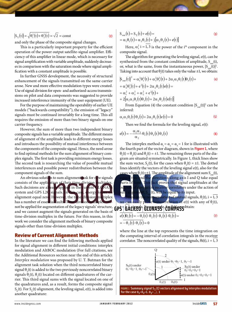
The interplex method α1 = α2 = α3 = 1 for is illustrated with the fourth part of the vector diagram, shown in figure 1, where θ1(t) = θ2(t) and θ3(t) = ±1. The remaining three parts of the dia-gram are situated symmetrically. In Figure 1, thick lines show the sum vector, SΣ(t), for the cases when θ3(t) = ±1. The dotted lines identify the vectors of the leveling signal e(t), also for the cases when θ3(t)=±1. The amplitude of the alignment sum Sout(t), equals two and the directions along axis I and Q take equal parts of time. This fact proves that signal amplitudes at the outputs of navigation receiver correlators under the action of sum alignment, Sout(t), will be equal to its input.

Based on the noncorrelation of mutual signals, θi(t), we can easily prove noncorrelation of e(t) with any of θi(t),

, signals. For example, for θi(t) we obtain:

where the line at the top represents the time integration on the computing interval of correlation integrals in the receiver correlator. The noncorrelated quality of the signals, θi(t),

FIGURE 1 Summary signal SΣ(t) vectors alignment by interplex modulation for the case 01=02=1. 03= _|_ 1


with each other and their noncorrelation with the leveling signal, e(t), supports the absence of mutual interferences and interferences that occur due to the input of the leveling signal.

The power of the leveling signal, e(t), defines the losses related to alignment. The power is equal to Pe = (α1α3/α2)

2. For the quantitative characteristic we use the loss coefficient on alignment (LCA), η, which is equal to the power ratio of the leveling signal to the power of the equalized signal.

We can easily show that the LCA does not depend on absolute values of αi, but only on relative values,

. For this purpose we should divide the numerator and the denominator in (8) by

that reduces to (9):

Equation (9) for LCA allows us to optimize the composite signal, SΣ(t), for alignment. Actually, η monotonously reduces with augmentation, μ2, which identifies the fractional power of the signal coincident on the quadrature with the leveling signal, e(t). Hence, under the given power of the component signals, the signal with the maximum , should be the unique one on its quadrature in the composite signal SΣ(t), i.e.,

where k ≠ m ≠ i. The LCA of such a signal is

Three-component signals of the L1 GPS band and E1-L1-E2 Galileo band, which apply the interplex modulation meet the optimality condition. Actually, as discussed in the article by E. Robeyrol et alia, in the GPS power ratio, =0 dB: 0.5 dB: -3dB, i.e., the C/A signal with maximum power =0.5dB is the unique one on its quadrature. This particular case of inter-plex modulation, suggested by P. Dafesh et alia, received its own name CASM (coherent adaptive subcarrier modulation). In Galileo, for alignment of the CBOC-signal (composite binary offset carrier) — which is the original version of the BOC signal — at power ratio =1:2:1, the second component PRS signal has been singled out into a special quadrature, and the data and pilot components of the open access signal combine on a common quadrature.

Normalization of μi coefficients in (9) allows us to present them as the points on the unit sphere by means of the angles, which assign the latitude B and longitude L.

at, . This allows us to present depen-dence LCA from αi (8) via B and L. This relationship in the form of level lines is shown in figure 2.

We can specify three fields. In each field one of, αk, is maximal. The maximum value of LCA, η=0.25 at alignment with the method of interplex modulation will be at the power equality of the composite signals, (μ1=μ2=μ3), when

and L=π/4. Such a value of LCA cannot be considered accept-able because the power of the aligned and useful component signals is equal. That is why both GPS and Galileo systems chose component signals that are not equal in power. From (8) it follows that η=0.177 for GPS, and η=1/9 ≈0.1 for Galileo. This is less than η=0.25 under the condition of equal power. Hereafter, we will provide several options that reduce the losses on the alignment of equal-strength signals if we combine these signals on the same or nearby frequencies.

AltBOC modulation was developed for the transfer of two independent pairs of orthogonal binary signals, located on close carrier frequencies, via common antenna. If we amplify these signals separately, we should carry out band-pass filter-ing of each one before their integration for emission. Due to the closeness of carrier frequencies, such a filtration leads to inadmissible distortions in emitted signals. These distortions are removed by means of common signal generation from two independent signals followed by signal amplification in one power amplifier. This option provides the necessary common signal alignment.

AltBOC modulation is used in the Galileo system for emis-sion of two independent signals over the range E5a-E5b on different carrier frequencies. The authors who recommended

workIng papers

FIGURE 2 Dependence LCA from B and L for interplex modulation

1.5

1

0.5

0

B

0 0.5 1 1.5L


AltBOC modulation describe it in the papers by L. Lestarquit et alia and G. W. Hein et alia and listed in Additional References) as a particular method, which leads to amplitude stability of the leveling signal. The main principle of AltBOC modulation is not described and remains unclear.

The foregoing review demonstrates the unsatisfactory status of sum alignment theory of navigation signals in GNSS. The various alignment methods do not have a common theoretical basis and have been developed by the designers based on an intuitive approach. Alignment principles serving as the basis of AltBOC modulation remain unclear.

synthesis of alignment Methods Based on LCa Minimum CriterionIn the general case, the composite signal, which should be aligned, can be noted as

where ψΣ(t) is the phase of the composite signal; Si(t), is the ith component of the composite signal

is the power of the ith component, θi(t)=±1; ψi(t) is the vector angle in the complex plane with the values θi(t) = ±1 along it; and М is the number of components in the composite signal, SΣ(t).

Let us introduce the aligned composite signal, Sal(t), like this:

where Se(t) is the leveling signal which is defined by amplitude C and phase φ(t). Taking into account (13) and (14), LCA can be shown thus:

where

Minimum LCA along the amplitude C with fixed value φal(t) can be found by evaluating the following equation:

Hence, we obtain:

Substituting (18) into (15) yields:

In the general case, , and equality can be reached only when the value of x equals 0. Hence, taking (16) into account, the minimum (19) according to φal(t) can be reached in this way:

and in this case,

From (20) and ( 21) it follows that the optimal alignment method should keep constant the phase of the composite signal, SΣ(t) (13), at every moment and align the signal’s amplitude to that value which is equal to the relation of the average power of the composite signal to the average value of its amplitude. From the basic property

and , it follows that in the general case, amplitude of the optimally aligned composite signal is more than the aver-age amplitude Copt of the composite signal, SΣ(t).

Clearly, then, only the relative correlation between ampli-tudes SΣ(t) and Sal(t) is important and not the absolute value of the amplitude С of the aligned signal. For this reason, we will take on a value Copt = 1. With this proviso, we have proved a very simple, but not quite expected result: generation of the optimally aligned composite signal is carried out by means of a simple and well known procedure of tight restriction of the composite signal:

where, for the complex value,

Note that the aforementioned method of optimum align-ment does not define the aligned composite signal Sal(t) (12) on time intervals, where SΣ(t) = 0. The exit from this uncertain situation can be inferred from physical reasoning. On time


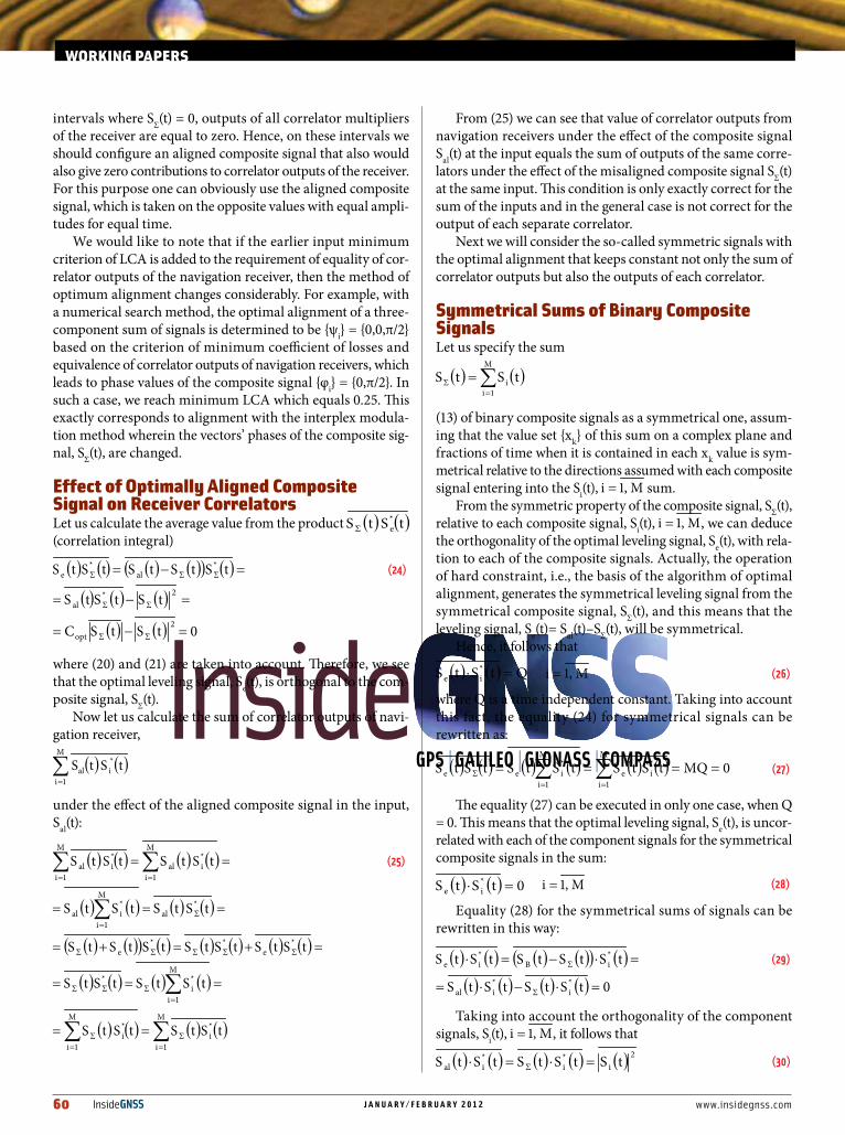
intervals where SΣ(t) = 0, outputs of all correlator multipliers of the receiver are equal to zero. Hence, on these intervals we should configure an aligned composite signal that also would also give zero contributions to correlator outputs of the receiver. For this purpose one can obviously use the aligned composite signal, which is taken on the opposite values with equal ampli-tudes for equal time.

We would like to note that if the earlier input minimum criterion of LCA is added to the requirement of equality of cor-relator outputs of the navigation receiver, then the method of optimum alignment changes considerably. For example, with a numerical search method, the optimal alignment of a three-component sum of signals is determined to be {ψi} = {0,0,π/2} based on the criterion of minimum coefficient of losses and equivalence of correlator outputs of navigation receivers, which leads to phase values of the composite signal {φi} = {0,π/2}. In such a case, we reach minimum LCA which equals 0.25. This exactly corresponds to alignment with the interplex modula-tion method wherein the vectors’ phases of the composite sig-nal, SΣ(t), are changed.

effect of optimally aligned Composite signal on receiver CorrelatorsLet us calculate the average value from the product (correlation integral)

where (20) and (21) are taken into account. Therefore, we see that the optimal leveling signal, Se(t), is orthogonal to the com-posite signal, SΣ(t).

Now let us calculate the sum of correlator outputs of navi-gation receiver,

under the effect of the aligned composite signal in the input, Sal(t):

From (25) we can see that value of correlator outputs from navigation receivers under the effect of the composite signal Sal(t) at the input equals the sum of outputs of the same corre-lators under the effect of the misaligned composite signal SΣ(t) at the same input. This condition is only exactly correct for the sum of the inputs and in the general case is not correct for the output of each separate correlator.

Next we will consider the so-called symmetric signals with the optimal alignment that keeps constant not only the sum of correlator outputs but also the outputs of each correlator.

symmetrical sums of Binary Composite signalsLet us specify the sum

(13) of binary composite signals as a symmetrical one, assum-ing that the value set {xk} of this sum on a complex plane and fractions of time when it is contained in each xk value is sym-metrical relative to the directions assumed with each composite signal entering into the Si(t), sum.

From the symmetric property of the composite signal, SΣ(t), relative to each composite signal, Si(t), , we can deduce the orthogonality of the optimal leveling signal, Se(t), with rela-tion to each of the composite signals. Actually, the operation of hard constraint, i.e., the basis of the algorithm of optimal alignment, generates the symmetrical leveling signal from the symmetrical composite signal, SΣ(t), and this means that the leveling signal, Se(t)= Sal(t)–SΣ(t), will be symmetrical.

Hence, it follows that

where Q is a time independent constant. Taking into account this fact, the equality (24) for symmetrical signals can be rewritten as:

The equality (27) can be executed in only one case, when Q = 0. This means that the optimal leveling signal, Se(t), is uncor-related with each of the component signals for the symmetrical composite signals in the sum:

Equality (28) for the symmetrical sums of signals can be rewritten in this way:

Taking into account the orthogonality of the component signals, Si(t), , it follows that

workIng papers


i.e., at the outputs of correlators in the case of the influence of an optimally aligned symmetrical sum, we receive the same value as in the case of influence for a non-aligned sum, SΣ(t). This property of the symmetrically aligned sums of signals gen-erally is not incident to arbitrary asymmetrically aligned sums with signal power rescheduling at the outputs of correlators corresponding to components of the sum.

In a later section, we consider the method of construction of the symmetric sums of signals (symmetrization method) from any asymmetrical sums.

The symmetrical sums of composite binary signals with optimal alignment represent the signals with phase modula-tion. Therefore, for convenience later on, we will refer to these as multicomponent signals with phase modulation (MSPM).

examples of symmetrical sums of Complex Binary signalsLet us consider the following example of a three-component symmetrical MSPM:

The vector diagram of this signal is shown in figure 3.The distribution of values of a three-component MSPM is

shown in figure 4. Comparing Figures 3 and 4 we can see the symmetry of distribution of the sum which consists of three signals, Si(t), relative to the value of each signal entering into the sum, SΣ(t).

The values of the aligned signal are shown in Figure 4 with asterisks located on the circle of radius two. In six cases out of eight, these values coincide with the initial composite signal, SΣ(t).

As shown in Figure 4, six values of the composite signal lie on the radius circle 2 symmetrically with regard to each of three directions,

defined by the component signals. The portion of time р when the composite signal takes on each of these values (i.e., the probability value), is equal to pi = 1/8, . Two more val-ues in the distribution generated by values θ1 = θ2 = θ3 = ±1, with a relative part of time pi = 1/8, i = 7, 8 are equal to x7 = x8 = 0. Using these values, we can find the average value of the amplitude

and average power of the composite signal

Hence, from (16) and (17),

Provided that SΣ(t) = 0, (x7 = x8 = 0), as noted above, the aligned signal can have any phase if its summary contribution (integral) equals zero for the time frame when SΣ(t) = 0. (This is one quarter of the entire integration time).

As examples of a four-component MSPM, we will consider two composite signals:

Vector diagrams of these signals are shown in figures 5a and 5b.

FIGURE 3 Vector diagram of three-component symmetrical MSPM

FIGURE 4 Distribution of values of three-component symmetrical MSPM

FIGURE 5 Vector diagrams of four-component symmetrical MSPM


The value distribution of the sums of the two four-compo-nent MSPMs in Figure 5 is shown with asterisks in figures 6a and 6b. From comparison of the latter figures, we can see the symmetry of distributions of the sums from four signals, Si(t),

relative to the value of each signal entering into sums and .

The general number of values in both cases equals 16. How-ever, a portion of the values is repeated twice, and the zero value is repeated four times.

Let us consider the parameters of the first composite signal, , which is shown in Figure 5a.

The values of this signal distributed on two circles is shown in Figure 6a. The radius of the larger circle can be found as signal amplitude, for example, when θ1 = θ2 = θ3 = θ4 = 1,

The radius of the smaller circles has the signal amplitude for the case when θ1 = θ3 = θ4 = 1, θ2 = –1,

Hence, the average amplitude value is equal to

The average value of signal power, as it must be for the sum of 4 noncorrelated (orthogonal) signals, is equal to:

Values of the aligned sum of signals are shown in Figure 6a with the asterisks located in circles. The aligned signal takes on one of eight values with equal probability.

Let us now calculate the characteristics of the second com-posite signal, . According to Figure 6b, four of its values are located at zero, two times four values (total eight) are located on a circle of small radius and four single values are located on a big circle.

The radius of a small circle can be found, for example, as the amplitude of a signal when θ1 = θ2 = 1, θ3 = 1, θ4 = –1. Obvi-ously, the corresponding amplitude will be equal to two. The radius of a big circle can be found as the amplitude of a signal when θ1 = θ2 = θ3 = θ4 = 1. Thus, we can easily see that the cor-

responding amplitude is equal to . From here we can find and :

whence we can find

The second four-component signal MSPM, , is clearly almost two times worse than that of the first signal on LCA.

The considered examples of three- and four-component MSPM signals show how to construct five-, six-, etc., compo-nent MSPM signals.

symmetrization Method of arbitrary sum signalsWe pointed out earlier that for asymmetrical sums of signals, in the course of carrying out the optimal alignment, the ener-gy redistribution of the aligned signal between the correlators occurs. Let us now consider the optimal alignment of a three-component asymmetrical sum as an example:

In figure 7 we can see the fourth part of phase diagram of the initial sum SΣ(t) which is shown with asterisks. The other three parts are located symmetrically. The vectors of the signals , are shown with the thick lines. The vectors of the signals Si(t)

resulting from the optimal alignment are shown with the dotted lines. From Figure 7 we can easily obtain the signals’ amplitudes at the correlators’ outputs of the navigation receiver

workIng papers

FIGURE 6 Value distribution of the sums of two four-component MSPM


i.e., the power of the third signal, occupying quadrature Q, at the output of the corresponding correlator is larger by 2.62 than the power of the first and the second signals combined on the I quadrature.

However, the LCA for such an aligned three-component sum is notably less than the LCA of the symmetrical three-component sum, presented in Figure 3, which is equal to 0.25. In fact, according to Figure 7, the spectrum of values |SΣ(t)| con-sists of two equiprobable “conditions” . Hence, we obtain

From orthogonality of composite signals, Si(t), , it fol-lows that

From here, according to (20), LCA for the sum presented in Figure 7 is equal to

It is less by almost half than 0.25, the LCA obtained for the symmetrical three-component sum presented in Figure 3.

One can propose a symmetrization method of the initial sum, SΣ(t). For this purpose, instead of SΣ(t) we will form in turn one of three signals:

In this regard, each of component signals, θi(t), is situated on quadrature Q for an equal part (one third) of the time and take up the quadrature I in combination with another component signal for two thirds of the time. In figure 8 we can see the phase diagrams of a signal (34) in reference to the direc-tion that is given with an arbitrarily chosen component, θ*(t).

Given such a direction, in Figure 8 we use the direction of horizontal axes. In Figure 8a we can see the relative phase diagram of the signal (31) for two thirds of the time, when the component θ*(t) is situated on quadrature I. Figure 8a shows the portions of time when a composite signal vector will be in the time intervals of the component θ*(t) location on the quadra-ture I. The relative phase diagram of the signal (31) is shown in

Figure 8b for one-third of the time when its component θ*(t) is situated on the quadrature Q. Figure 8b identifies the portions of time when a composite signal vector will be in the time inter-vals of component θ*(t) location on the quadrature Q.

Figure 8c shows the total relative phase diagram of an MSPM signal (from Equation 31) The fractional values near the asterisks in Figure 8c identify the portions of time that a com-posite signal vector will be in reference to the direction given by the component θ*(t). We see that the total phase diagram is symmetrical in relation to the direction given by the arbitrarily chosen component θ*(t). It then follows that the signal (31) is symmetrical and, hence, demonstrates for this signal the prop-erty of equivalence proved earlier of aligned signal action on each receiver correlator by the action of the nonaligned signal (with the power reduced by 12.73 percent) and absent of distor-tions from the action of aligned signal.

Generally, for an arbitrary M-component signal,

the symmetrization procedure consists of forming the time mix of signals with all combinations from the M component

FIGURE 7 Phase diagram of three-component aligned sum

FIGURE 8 Phase diagram of symmetrized three-component sum


signals on the two-quadrature axis. The number of these is generally .

Unfortunately, the permutation of component signals between the quadratures assumed in the symmetrization meth-od is impossible for existing GNSS signals, and in the general case for the users it is equivalent to changing a signal with two-phase modulation (BPSK) to a signal with four-phase modu-lation (QPSK). A later section considers from a GNSS user’s perspective the particular variants of symmetrization that are not brought to such modification of two or three signals.

In figure 9 we provide in the form of level lines the depen-dence of LCA obtained by simulation for a symmetrized three-component signal, α1θ1(t) + α3θ3(t) +jα2θ2(t), in coordinates B and L, introduced in the first section of this article.

From Figure 9 we see that the LCA maximum value is reached at and L = π/4, which is equivalent to α1 = α2 = α3, and equals η=0.1273.

Comparing Figure 9 with LCA ηint (for interplex modula-tion), we see that for all correlations, α1, α2, α3, LCA ηs (the sym-metrized signals with optimal alignment) have become quite less than at interplex modulation.

If we have equal powers of component signals, we can reach almost double gain (0.1273 and 0.25). For the accepted ratio in Galileo, , we get ηint = 1/9 ≈ 0.11 against

For GPS, if , ηint = 1/6 ≈ 0.167 against

optimal phases for Multi-Component signal sums Using Minimum LCa CriterionBy the method of numerical search and also using numerical sorting of all phases ψi, we found the optimal value of the phas-es for three- and four-component sums of the signals providing the minimum value of LCA in the course of optimal alignment

as described earlier. For three-component signals at any ratio of amplitudes, only one minimum is reached at {ψi} = {0, 0, π/2} or any other permutation of phase components (asymmetrical signal). Thus for equal amplitudes, the minimum LCA value is equal to η =0.1273.

Four-component signals have two similar minimums: η1=0.1464, obtained if {ψi} = {0, π/4, π/2, 3π/4} (symmetric sum), and η2=0.1432, achieved if {ψi} = {0, 0, 0, π/2} or at any other combination with the arrangement of three components on one quadrature and one component on another one (asym-metrical sum). The preferred relationship should be the first phase distribution, {ψi} = {0, π/4, π/2, 3π/4}, as it is symmetri-cal and the loss coefficient, η1=0.1464, corresponding to this arrangement is insignificantly less than the absolute minimum η2=0.1432.

synthesis of altBoC signalAltBOC modulation was developed for the transmission of two independent pairs of orthogonal binary signals

where θ1(t) = θ11(t) + jθ12(t) and θ2(t) = θ21(t) + jθ22(t) are complex binary signals with two quadratures, θ11(t), θ12(t), θ21(t), θ22(t) taking the value ±1, emitted on the different, but nearby car-rier frequencies ω1, ω2, (ω1 < ω2), through the common antenna. Given that θ1(t), θ2(t) are binary, their phases take the values, (2k + 1) . π/4, k = .

Let us consider the optimal LCA minimum AltBOC-like signal as a generalization of the optimal four-component MSPM signal considered in previous sections with η=0.1464. It is not difficult to ascertain that this coincides with

within the substitution θ11 = θ1, θ12 = θ3, θ21 = θ2, and θ22 = θ4. If we represent

where a clear connection ki with θi1, θi2, is defined by Table 1,

θi1 1 –1 1 –1

θi2 1 1 –1 –1

ki 0 1 3 2

TABLE 1 Connection ki with θi1, θi2

SΣ(t) can be presented as

For generation of an AltBOC-like signal, the components θ1(t) and θ2(t) should be shifted on the frequencies ω1 and ω2, i.e., the signal becomes:

FIGURE 9 Dependence LCA from B and L for symmetrized three-component signal

1.5

1

0.5

0

B

0 0.5 1 1.5L

workIng papers


where δi(t) are approximations of the linearly varying phase, ωi(t), of frequency shift, which we will soon choose. Removing the average geometrical of summands from the square brack-ets, we now have:

where k+ = k1 + k2, k- = k2 – k1, δ+(t) = (δ2(t) + δ1(t))/2, δ–(t) = δ2(t) – δ1(t))/2. The value of signal amplitude is equal to

Taking into account that |cos(x)| has the period π, the sum-mand under a cosine can be considered modulo π and we can suppose that k– = mod(k2, – k1,4), that is takes values 0…3. For equally probable values, θij(t), i, j = , the distribution of k1 and k2, is obviously uniform in . It is not difficult to make sure that modulo k– are also equiprobable. Summation with an arbitrary constant maintains a probability distribution that is equiprobable.

This implies that, if δ–(t) is divisible by π/4, then the prob-ability distribution of the modulo 4 cosine argument does not change. Distribution of |SΣ(t)| at that point remains the same as well, i.e., the optimal value LCA = 0.1464. This is why k– has four equally probable values 0, 1, 2, 3. In other words, we should accept the step approximation of phase δ–(t) with step values equal to π/4 (figure 10):

where the step height is defined with difference frequency f– = f2 – f1 – (ω2 – ω1)/2π

Total phase does not influence amplitude distribution, therefore it is naturally accepted as equal to δ+(t) = (ω2 + ω1) . t/2. In this connection, δ2,1(t) = (ω2 + ω1) . t/2 + δ–(t).

Strict restriction of a summary signal leads to an expression for the aligned signal depending on discrete parameters θ1 and θ2 (through k– and k+) and the step number (discrete time, ).

where cr(x) = sign(cos(x)).The AltBOC signal presentation given by the European

GNSS Open Service Signal in Space Interface Control Docu-ment (OS SIS ICD) generalizes the case of nonzero frequency by means of the following expression:

From (42) it follows that the phase set number (one out of eight) is determined by the expression

The restriction on the set of frequencies f1 and f2 arises from the obvious requirement of the integer number of steps, ri, on the length τi of the symbols of code sequences θ1 and θ2

Integration of conditions (41) and (44) sets the restriction on the choice of frequency difference

Having referred to a particular case of AltBOC signal real-ized in a signal of frequency band E5 for Galileo, where f2 + –f1 = 15fb, τ1 = τ2 = 15fb = 1/10fb, we determine that f2 – f1 = 30fb, f2 + f1 = 0, h = 1/4(f2 – f1) = 1/20fb. The condition in (45) is obvi-ously fulfilled, and r1 = r2 = 12.

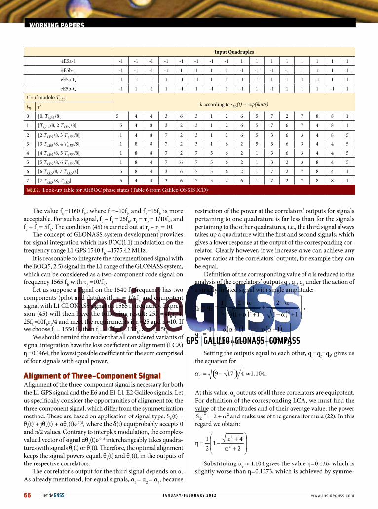
Expression (42) defines the phase value state. Comparison of k values for all θ1(t), θ2(t), and to Table 6 in the Galileo OS SIS ICD —republished here as Table 2 — demonstrates their full coincidence. This shows that the E5 Galileo signal can be considered as a particular case of the aligned four-component signal.

For the prospective signals L3 and L5 in the GLONASS system, we propose frequencies that are equal to 1175 fb and 1150 fb (fb = 1.023 MHz), respectively, and we also apply two-component signals with symbol duration of ranging code τ = 1/10fb. The application of the AltBOC signal with its symmetri-cal subcarriers is assumed to generate the carrier on f0=1162.5 fb frequency. Such a value is inconvenient for the frequency synthesizer and gives rise to increasing phase noise within that system element.

FIGURE 10 Stepped approximation of phase δ–(t)


The value f0=1160 fb, where f1=–10fb and f2=15f b is more acceptable. For such a signal, f2 – f1 = 25fb, τ1 = τ2 = 1/10fb, and f2 + f1 = 5fb. The condition (45) is carried out at r1 – r2 = 10.

The concept of GLONASS system development provides for signal integration which has BOC(1,1) modulation on the frequency range L1 GPS 1540 fb =1575.42 MHz.

It is reasonable to integrate the aforementioned signal with the BOC(5, 2.5) signal in the L1 range of the GLONASS system, which can be considered as a two-component code signal on frequency 1565 fb with τ2 =10/fb.

Let us suppose a signal on the 1540 fb frequency has two components (pilot and data) with τ1 = 1/4fb and equipotent signal with L1 GLONASS signal on 1565 fb frequency. Expres-sion (45) will then have the following result: 25f b=4f br1/4, 25fb=10fbr2/4 and meet the requirements if r1=25 and r2=10. If we choose f0 = 1550 fb, then f1=-10 fb, f2=15 fb, and f+=5fb.

We should remind the reader that all considered variants of signal integration have the loss coefficient on alignment (LCA) η =0.1464, the lowest possible coefficient for the sum comprised of four signals with equal power.

alignment of Three-Component signal Alignment of the three-component signal is necessary for both the L1 GPS signal and the E6 and E1-L1-E2 Galileo signals. Let us specifically consider the opportunities of alignment for the three-component signal, which differ from the symmetrization method. These are based on application of signal type: SΣ(t) = θi(t) + jθ2(t) + αθ3(t)e

jδ(t), where the δ(t) equiprobably accepts 0 and π/2 values. Contrary to interplex modulation, the complex-valued vector of signal αθ3(t)e

jδ(t) interchangeably takes quadra-tures with signals θ1(t) or θ2(t). Therefore, the optimal alignment keeps the signal powers equal, θ1(t) and θ2(t), in the outputs of the respective correlators.

The correlator’s output for the third signal depends on α. As already mentioned, for equal signals, α1 = α2 = α3, because

restriction of the power at the correlators’ outputs for signals pertaining to one quadrature is far less than for the signals pertaining to the other quadratures, i.e., the third signal always takes up a quadrature with the first and second signals, which gives a lower response at the output of the corresponding cor-relator. Clearly however, if we increase α we can achieve any power ratios at the correlators’ outputs, for example they can be equal.

Definition of the corresponding value of α is reduced to the analysis of the correlators’ outputs q1, q2, q3 under the action of a strictly limited signal with single amplitude:

Setting the outputs equal to each other, q1=q2=q3, gives us the equation for

At this value, αe outputs of all three correlators are equipotent. For definition of the corresponding LCA, we must find the value of the amplitudes and of their average value, the power

and make use of the general formula (22). In this regard we obtain:

Substituting αe ≈ 1.104 gives the value η=0.136, which is slightly worse than η=0.1273, which is achieved by symme-

workIng papers

Input Quadruples

eE5a-1 -1 -1 -1 -1 -1 -1 -1 -1 1 1 1 1 1 1 1 1

eE5b-1 -1 -1 -1 -1 1 1 1 1 -1 -1 -1 -1 1 1 1 1

eE5a-Q -1 -1 1 1 -1 -1 1 1 -1 -1 1 1 -1 -1 1 1

eE5b-Q -1 1 -1 1 -1 1 -1 1 -1 1 -1 1 1 1 -1 1

t' = t' modolo Ts,E5k according to sE5(t) = exp(jkπ/r)iTs t'

0 [0, Ts,E5 /8[ 5 4 4 3 6 3 1 2 6 5 7 2 7 8 8 1

1 [Ts,E5 /8, 2 Ts,E5 /8[ 5 4 8 3 2 3 1 2 6 5 7 6 7 4 8 1

2 [2 Ts,E5 /8, 3 Ts,E5 /8[ 1 4 8 7 2 3 1 2 6 5 3 6 3 4 8 5

3 [3 Ts,E5 /8, 4 Ts,E5 /8[ 1 8 8 7 2 3 1 6 2 5 3 6 3 4 4 5

4 [4 Ts,E5 /8, 5 Ts,E5 /8[ 1 8 8 7 2 7 5 6 2 1 3 6 3 4 4 5

5 [5 Ts,E5 /8, 6 Ts,E5 /8[ 1 8 4 7 6 7 5 6 2 1 3 2 3 8 4 5

6 [6 Ts,E5/8, 7 Ts,E5/8[ 5 8 4 3 6 7 5 6 2 1 7 2 7 8 4 1

7 [7 Ts,E5 /8, Ts,E5[ 5 4 4 3 6 7 5 2 6 1 7 2 7 8 8 1

TABLE 2. Look-up table for AltBOC phase states (Table 6 from Galileo OS SIS ICD)


trization, but essentially better than η=0.25, as in interplex modulation.

A function selection δ(t) remains to be concretized. Two possible selections are obvious. The first one appears to be a convenient alternative (or expansion) of the AltBOC-like signal for generation of the double frequency three-component signal. For this purpose, we should choose

which is equivalent to the phase step approximation +2π f t of the third signal with frequency shift f = ±1/4h. As a result of such a selection for δ(t) we receive the integration of three binary phase signals (BPSK), with one of these signals shifted relative to the two others on frequency, f = ±1/4h. From the user’s point of view, these three signals will have equal power.

The second selection of δ(t) can be used if the frequency shift of the third signal is unacceptable. In this case

where sr(x)=sign(sin(x)) and δ(t) takes the value 0 or π/2 in alternating fashion. In this case, the third signal becomes the quadrature phase signal (QPSK), but the first and the second ones remain the usual BPSK signals.

ConclusionThe theory of optimal alignment of the GNSS navigation signals sum is developing. A review of applicable alignment methods is presented. Alignment methods for the synthesis of summarized signals on the LCA minimum criterion is devel-oped. Examples of sums of composite signals are considered. Symmetrization methods of arbitrary signal sums are also con-sidered. Concrete examples of new GLONASS signal synthesis are proposed.

additional resources[1] Avila-Rodriguez, J.-A. “The MBOC Modulation: The Final Touch to the Galileo Frequency and Signal Plan,” Proceedings of the 20th International Technical Meeting of the Satellite Division of The Institute of Navigation (ION GNSS 2007), Fort Worth, Texas USA, September 25–28, 2007

[2] Betz, J., “The Offset Carrier Modulation for GPS Modernization,” Proceed-ings of The Institute of Navigation 1999 National Technical Meeting, San Diego, California USA, January 1999

[3] Butman, U. T., “Interplex – An efficient Multichannel PSK/PM Telemetry System,” IEEE Transactions on Communication, Vol. 20, No. 3, June 1972

[4] CNES Technical Note DTS/AE/TTL/RN – 2003-48, “Spectral Control with Constant Envelope Modulations Application to Galileo BOC Signals in E2-L1-E1,” 2003

[5] Dafesh, P. A., S. Lazar, T. M. Nguyen, “Coherent Adaptive Subcarrier Mod-ulation (CASM) for GPS Modernization,” Proceedings of the 1999 National Technical Meeting of The Institute of Navigation (ION NTM 1999), San Diego, California USA, January 1999

[6] European GNSS (Galileo) Open Service, Signal in Space Interface Control Document, European Union, 2010

[7] Global Navigation Satellite System (GLONASS) Interface Control Document, (Edition 5.1), http://rniikp.ru/ru/pages/about/publ/ikd51ru.pdf

[8] Hein, G. W., J. Godet, J.-L. Issler, J.-C. Martin, P. Erhard, R. Lucas-Rodri-guez, T. Pratt, “Status of Galileo Frequency and Signal Design,” Proceedings of ION GPS 2002, Portland, OR, September 24–27, 2002

[9] Hein, G. W., “A Candidate for the Galileo L1 OS Optimized Signal,” Proceed-ings of the 18th International Technical Meeting of the Satellite Division of The Institute of Navigation (ION GNSS 2005), September 23–16, 2005

[10] Ipatov, V.P., Shebshaevich B.V. “Spectrum-Compact Signals. A Suitable Option for Future GNSS,” Inside GNSS. Vol. 6, No 1, pp.47–53, January/Febru-ary 2011

[11] Lestarquit, L., G. Artand, L.-L. Issler, “AltBOC for Dummies or Everything You Always Wanted to Know About AltBOC,” Proceedings of the 21st Interna-tional Technical Meeting of The Institute of Navigation (ION GNSS 2008), Savannah, Georgia USA, September 16–19, 2008

[12] Navstar Global Positioning System, Interface Specification, IS-GPS-200, Revision D, IRN-200D-001, Navstar GPS Space Segment/Navigation User Interfaces, http://www.naic.edu/~phil/rfi/gps/AFD-070803-059-1.pdf, March 7, 2006

[13] Robeyrol, E., C. Macabiau, L. Ries, J. L. Issler, M. L. Bouchet, “Interplex Modulation for Navigation Systems at the L1 Band,” Proceedings of the 2006 National Technical Meeting of The Institute of Navigation (ION NTM 2006), Monterey, CA, January 18–20, 2006

authorsVladimir Kharisov is the science director of JSC “VNIIR Progress” and a professor of the Zhukovsky Air Force Engineering Academy. He has developed signal theory for more than 30 years and has published more than 150 papers and several monographs in signal theory and satellite navigation. More recent-ly, he has actively worked on developing new code

division GLONASS signals.

Alexander Povalyaev is the deputy head of the division in the JSC “Russian Space Systems” and is a professor at the Moscow Aviation Institute. He has developed methods and algorithms for GNSS carrier phase mea-surements processing for more than 30 years and has published more than 50 papers as well as a mono-graph in satellite navigation. In recent years, he has

actively worked on developing new code division GLONASS signals.

Guenter W. Hein serves as the editor of the Working Papers column. He is head of the Galileo Operations and Evolution Department of the European Space Agency. Previously, he was a full professor and direc-tor of the Institute of Geodesy and Navigation at the University FAF Munich. In 2002 he received the pres-tigious Johannes Kepler Award from the U.S. Institute

of Navigation (ION) for “sustained and significant contributions to satellite navigation.” He is one of the CBOC inventors.

Documents

workIng papers Optimal a ligning of the Sums of …signals must be continued invariably for a long time. This all requires the emission of more than two binary signals on one carrier