Embed Size (px)
Citation preview

Workload Design: Selecting Representative Program-Input Pairs
Lieven Eeckhout Hans Vandierendonck Koen De BosschereDepartment of Electronics and Information Systems (ELIS), Ghent University, Belgium
E-mail:�leeckhou,hvdieren,kdb � @elis.rug.ac.be
Abstract
Having a representative workload of the target domainof a microprocessor is extremely important throughout itsdesign. The composition of a workload involves two issues:(i) which benchmarks to select and (ii) which input datasets to select per benchmark. Unfortunately, it is impossi-ble to select a huge number of benchmarks and respectiveinput sets due to the large instruction counts per benchmarkand due to limitations on the available simulation time. Inthis paper, we use statistical data analysis techniques suchas principal components analysis (PCA) and cluster anal-ysis to efficiently explore the workload space. Within thisworkload space, different input data sets for a given bench-mark can be displayed, a distance can be measured betweenprogram-input pairs that gives us an idea about their mu-tual behavioral differences and representative input datasets can be selected for the given benchmark. This method-ology is validated by showing that program-input pairs thatare close to each other in this workload space indeed ex-hibit similar behavior. The final goal is to select a limitedset of representative benchmark-input pairs that span thecomplete workload space. Next to workload composition,there are a number of other possible applications, namelygetting insight in the impact of input data sets on programbehavior and profile-guided compiler optimizations.
1 Introduction
The first step when designing a new microprocessor isto compose a workload that should be representative for theset of applications that will be run on the microprocessoronce it will be used in a commercial product [1, 7]. A work-load then typically consists of a number of benchmarks withrespective input data sets taken from various benchmarkssuites, such as SPEC, TPC, MediaBench, etc. This work-load will then be used during the various simulation runs toperform design space explorations. It is obvious that work-load design, or composing a representative workload, is ex-tremely important in order to obtain a microprocessor de-sign that is optimal for the target environment of operation.The question when composing a representative workload isthus twofold: (i) which benchmarks and (ii) which inputdata sets to select. In addition, we have to take into accountthat even high-level architectural simulations are extremely
time-consuming. As such, the total simulation time shouldbe limited as much as possible to limit the time-to-market.This implies that the total number of benchmarks and in-put data sets should be limited without compromising thefinal design. Ideally, we would like to have a limited setof benchmark-input pairs spanning the complete workloadspace, which contains a variety of the most important typesof program behavior.
Conceptually, the complete workload design space canbe viewed as a � -dimensional space with � the num-ber of important program characteristics that affect perfor-mance, e.g., branch prediction accuracy, cache miss rates,instruction-level parallelism, etc. Obviously, � will be toolarge to display the workload design space understand-ably. In addition, correlation exists between these vari-ables which reduces the ability to understand what programcharacteristics are fundamental to make the diversity in theworkload space. In this paper, we reduce the � -dimensionalworkload space to a � -dimensional space with ����� ( ���to ��� � typically) making the visualisation of the workloadspace possible without losing important information. Thisis achieved by using statistical data reduction techniquessuch as principal components analysis (PCA) and clusteranalysis.
Each benchmark-input pair is a point in this (reduced) � -dimensional space obtained after PCA. We can expect thatdifferent benchmarks will be ‘far away’ from each otherwhile different input data sets for a single benchmark willbe clustered together. This representation gives us an ex-cellent opportunity to measure the impact of input data setson program behavior. Weak clustering (for various inputsand a single benchmark) indicates that the input set has alarge impact on program behavior; strong clustering on theother hand, indicates a small impact. This claim is validatedby showing that program-input pairs that are close to eachother in the workload space indeed exhibit similar behavior.I.e., ‘close’ program-input pairs react in similar ways whenchanges are made to the architecture.
In addition, this representation gives us an idea whichinput sets should be selected when composing a workload.Strong clustering suggests that a single or only a few inputsets could be selected to be representative for the cluster.This will reduce the total simulation time significantly fortwo reasons: (i) the total number of benchmark-input pairsis reduced; and (ii) we can select the benchmark-input pairwith the smallest dynamic instruction count among all the

pairs in the cluster. The reduction of the total simulationtime is an important issue for the evaluation of micropro-cessor designs since todays and future workloads tend tohave large dynamic instruction counts.
Another important application, next to getting insightin program behavior and workload composition, is profile-driven compiler optimizations. During profile-guided op-timizations, the compiler uses information from previousprogram runs (obtained through profiling) to guide com-piler optimizations. Obviously, for effective optimizations,the input set used for obtaining this profiling informationshould be representative for a large set of possible inputsets. The methodology proposed in this paper can be usefulin this respect because input sets that are close to each otherin the workload space will have similar behavior.
This paper is organized as follows. In section 2, the pro-gram characteristics used are enumerated. Principal compo-nents analysis, cluster analysis and their use in this contextare discussed in section 3. In section 4, it is shown thatthese data reduction techniques are useful in the context ofworkload characterization. In addition, we discuss how in-put data sets affect program behavior. Section 5 discussesrelated work. We conclude in section 6.
2 Workload Characterization
It is important to select program characteristics that af-fect performance for performing data analysis techniquesin the context of workload characterization. Selectingprogram characteristics that do not affect performance,such as the dynamic instruction count, might discriminatebenchmark-input pairs on a characteristic that does not af-fect performance, yielding no information about the behav-ior of the benchmark-input pair when executed on a micro-processor. On the other hand, it is important to incorpo-rate as many program characteristics as possible so that theanalysis done on it will be predictive. I.e., we want stronglyclustered program-input pairs to behave similarly so that asingle program-input pair can be chosen as a representativeof the cluster. The determination of what program charac-teristics to be included in the analysis in order to obtain apredictive analysis is a study on its own and is out of thescope of this paper. The goal of this paper is to show thatdata analysis techniques such as PCA and cluster analysiscan be a helpful tool for getting insight in the workloadspace when composing a representative workload.
We have identified the following program characteris-tics:�
Instruction mix. We consider five instruction classes:integer arithmetic operations, logical operations, shiftand byte manipulation operations, load/store opera-tions and control operations.�Branch prediction accuracy. We consider the branchprediction accuracy of three branch predictors: a bi-modal branch predictor, a gshare branch predictor anda hybrid branch predictor. The bimodal branch pre-dictor consists of an 8K-entry table containing 2-bit
saturating counters which is indexed by the programcounter of the branch. The gshare branch predic-tor is an 8K-entry table with 2-bit saturating coun-ters indexed by the program counter xor-ed with thetaken/not-taken branch history of 12 past branches.The hybrid branch predictor [10] combines the bi-modal and the gshare predictor by choosing amongthem dynamically. This is done using a meta predictorthat is indexed by the branch address and contains 8K2-bit saturating counters.�Data cache miss rates. Data cache miss rates weremeasured for five different cache configurations: an8KB and a 16KB direct mapped cache, a 32KB anda 64KB two-way set-associative cache and a 128KBfour-way set-associative cache. The block size was setto 32 bytes.�Instruction cache miss rates. Instruction cache missrates were measured for the same cache configurationsmentioned for the data cache.�Sequential flow breaks. We have also measured thenumber of instructions between two sequential flowbreaks or, in other words, the number of instructionsbetween two taken branches. Note that this metric ishigher than the basic block size because some basicblocks ‘fall through’ to the next basic block.�Instruction-level parallelism. To measure the amountof ILP in a program, we consider an infinite-resourcemachine, i.e., infinite number of functional units, per-fect caches, perfect branch prediction, etc. In addition,we schedule instructions as soon as possible assum-ing unit execution instruction latency. The only de-pendencies considered between instructions are read-after-write (RAW) dependencies through registers aswell as through memory. In other words, perfect reg-ister and memory renaming are assumed in these mea-surements.
For this study, there are � � �program characteristics
in total on which the analyses are done.
3 Data Analysis
In the first two subsections of this section, we will dis-cuss two data analysis techniques, namely principal compo-nents analysis (PCA) and cluster analysis. In the last sub-section, we will detail how we used these techniques foranalyzing the workload space in this study.
3.1 Principal Components Analysis
Principal components analysis (PCA) [9] is a statisti-cal data analysis technique that presents a different viewon the measured data. It builds on the assumption thatmany variables (in our case, program characteristics) arecorrelated and hence, they measure the same or similarproperties of the program-input pairs. PCA computes new

variables, called principal components, which are linearcombinations of the original variables, such that all prin-cipal components are uncorrelated. PCA tranforms the� variables ����������������� into � principal components� ��� � ������ � with
��� ��� ��� ��� � � � � . This transforma-tion has the properties (i) � ����� � ���� � �!�"� � ��� � � ����� � � which means that
� � contains the most informa-tion and
� the least; and (ii) #%$�& � ��� � � � � � � �('*),+�.-which means that there is no information overlap betweenthe principal components. Note that the total variance in thedata remains the same before and after the transformation,namely � � � � � �!�"� � � � � � � � � � ���"� ��� � .
As stated in the first property in the previous paragraph,some of the principal components will have a high vari-ance while others will have a small variance. By removingthe components with the lowest variance from the analysis,we can reduce the number of program characteristics whilecontrolling the amount of information that is thrown away.We retain � principal components which is a significant in-formation reduction since � � � in most cases, typically� � to � � � . To measure the fraction of informationretained in this � -dimensional space, we use the amount ofvariance /0�21� � � � ���"� �3� �5476 /8� � � � � �!�"� � � �54 accounted forby these � principal components.
In this study the � original variables are the programcharacteristics mentioned in section 2. By examining themost important � principal components, which are linearcombinations of the original program characteristics, mean-ingful interpretations can be given to these principal com-ponents in terms of the original program characteristics. Tofacilitate the interpretation of the principal components, weapply the varimax rotation [9]. This rotation makes the co-efficients � � � either close to 9 1 or zero, such that the origi-nal variables either have a strong impact on a principal com-ponent or they have no impact. Note that varimax rotation isan orthogonal transformation which implies that the rotatedprincipal components are still uncorrelated.
The next step in the analysis is to display the variousbenchmarks as points in the � -dimensional space built up bythe � principal components. This can be done by computingthe values of the � retained principal components for eachprogram-input pair. As such, a view can be given on theworkload design space and the impact of input data sets onprogram behavior can be displayed, as will be discussed inthe evaluation section of this paper.
During principal components analysis, one can eitherwork with normalized or non-normalized data (the data isnormalized when the mean of each variable is zero andits variance is one). In the case of non-normalized data,a higher weight is given in the analysis to variables witha higher variance. In our experiments, we have used nor-malized data because of our heterogeneous data; e.g., thevariance of the ILP is orders of magnitude larger than thevariance of the data cache miss rates.
3.2 Cluster Analysis
Cluster analysis [9] is another data analysis techniquethat is aimed at clustering : cases, in our case program-
input pairs, based on the measurements of � variables, in ourcase program characteristics. The final goal is to obtain anumber of groups, containing program-input pairs that have‘similar’ behavior. A commonly used algorithm for doingcluster analysis is hierarchic clustering which starts with amatrix of distances between the : cases or program-inputpairs. As a starting point for the algorithm, each program-input pair is considered as a group. In each iteration of thealgorithm, the two groups that are most close to each other(with the smallest distance, also called the linkage distance)will be combined to form a new group. As such, closegroups are gradually merged until finally all cases will bein a single group. This can be represented in a so calleddendrogram, which graphically represents the linkage dis-tance for each group merge at each iteration of the algo-rithm. Having obtained a dendrogram, it is up to the userto decide how many clusters to take. This decision can bemade based on the linkage distance. Indeed, small linkagedistances imply strong clustering while large linkage dis-tances imply weak clustering.
How we define the distance between two program-inputpairs will be explained in the next section. To computethe distance between two groups, we have used the near-est neighbour strategy or single linkage. This means thatthe distance between two groups is defined as the smallestdistance between two members of each group.
3.3 Workload Analysis
The workload analysis done in this paper is a combina-tion of PCA and cluster analysis and consists of the follow-ing steps:
1. The � � �program characteristics as discussed in
section 2 are measured by instrumenting the bench-mark programs with ATOM [13], a binary instrumen-tation tool for the Alpha architecture. With ATOM, astatically linked binary can be transformed to an instru-mented binary. Executing this instrumented binary onan Alpha machine yields us the program characteris-tics that will be used throughout the analysis. Measur-ing these � � �
program characteritics was done forthe 79 program-input pairs mentioned in section 4.1.
2. In a second step, these ;�< (number of program-inputpairs) = �
( � � , number of program characteristics)data points are normalized so that for each programcharacteristic the average equals zero and the vari-ance equals one. On these normalized data points,principal components analysis (PCA) is done usingSTATISTICA [14], a package for statistical computa-tions. This works as follows. A 2-dimensional ma-trix is presented as input to STATISTICA that has 20columns representing the original program character-istics as mentioned in section 2. There are 79 rowsin this matrix representing the various program-inputpairs. On this matrix, PCA is performed by STATIS-TICA which yields us � principal components.

3. Once these � principal components are obtained, avarimax rotation can be done on these data for improv-ing the understanding of the principal components.This can be done using STATISTICA.
4. Now, it is up to the user to determine how many prin-cipal components need to be retained. This decision ismade based on the amount of variance accounted forby the retained principal components.
5. The � principal components that are retained can beanalyzed and a meaningful interpretation can be givento them. This is done based on the coefficients � � � , alsocalled the factor loadings, as they occur in the follow-ing equation
��� � � ��� � � � � � � , with��� � ��� ) � �
the principal components and � � � ��� - � � the orig-inal program characteristics. A positive coefficient � � �means a positive impact of program characteristic � �on principal component
���; a negative coefficient � � �
implies a negative impact. If a coefficient � � � is closeto zero, this means � � has (nearly) no impact on
� �.
6. The program-input pairs can be displayed in the work-load space built up by these � principal compo-nents. This can easily be done by computing
� � �� ��� � � � � � � for each program-input pair.
7. Within this � -dimensional space the Euclidean dis-tance can be computed between the various program-input pairs as a reliable measure for the way program-input pairs differ from each other. There are two rea-sons supporting this statement. First, the values alongthe axes in this space are uncorrelated since they aredetermined by the principal components which are un-correlated by construction. The absence of correla-tion is important when calculating the Euclidean dis-tance because two correlated variables—that essen-tially measure the same thing—will contribute a sim-ilar amount to the overall distance as an independentvariable; as such, these variables would be countedtwice, which is undesirable. Second, the variancealong the � principal components is meaningful sinceit is a measure for the diversity along each principalcomponent by construction.
8. Finally, cluster analysis can be done using the distancebetween program-input pairs as determined in the pre-vious step. Based on the dendrogram a clear view isgiven on the clustering within the workload space.
The reason why we chose to first perform PCA and sub-sequently cluster analysis instead of applying cluster anal-ysis on the initial data is as follows. The original variablesare highly correlated which implies that an Euclidean dis-tance in this space is unreliable due to this correlation as ex-plained previously. The most obvious solution would havebeen to use the Mahalanobis distance [9] which takes intoaccount the correlation between the variables. However,the computation of the Mahalanobis distance is based ona pooled estimate of the common covariance matrix whichmight introduce inaccuracies.
4 Evaluation
In this section, we first present the program-input pairsthat are used in this study. Second, we show the resultsof performing the workload analysis as discussed in sec-tion 3.3. Finally, the methodology is validated in sec-tion 4.3.
4.1 Experimental Setup
In this study, we have used the SPECint95 benchmarks(http://www.spec.org) and a database workloadconsisting of TPC-D queries (http://www.tpc.org),see Table 1. The reason why we chose SPECint95 insteadof the more recent SPECint2000 is to limit the simulationtime. SPEC opted to dramatically increase the runtimesof the SPEC2000 benchmarks compared to the SPEC95benchmarks which is beneficial for performance evaluationon real hardware but impractical for simulation purposes.In addition, there are more reference inputs provided withSPECint95 then with SPECint2000. For gcc (GNU C com-piler) and li (lisp interpreter), we have used all the referenceinput files. For ijpeg (image processing), penguin, spec-mun and vigo were taken from the reference input set. Theother images that served as input to ijpeg were taken fromthe web. The dimensions of the images are shown in brack-ets. For compress (text compression), we have adaptedthe reference input ‘14000000 e 2231’ to obtain differentinput sets. For m88ksim (microprocessor simulation) andvortex (object-oriented database), we have used the trainand the reference inputs. The same was done for perl (perlinterpreter): jumble was taken from the train input, andprimes and scrabbl were taken from the reference input;as well as for go (game): ‘50 9 2stone9.in’ from the traininput, and ‘50 21 9stone21.in’ and ‘50 21 5 stone21.in’from the reference input.
In addition to SPECint95, we used postgres v6.3 run-ning the decision support TPC-D queries over a 100MBBtree-indexed database. For postgres, we ran all TPC-Dqueries except for query 1 because of memory constraintson our machine.
The benchmarks were compiled with optimization level-O4 and linked statically with the -non shared flag for theAlpha architecture.
4.2 Results
In this section, we will first perform PCA on the datafor the various input sets of gcc. Subsequently, the samewill be done for postgres. Finally, PCA and cluster analy-sis will be applied on the data for all the benchmark-inputpairs of Table 1. We present the data for gcc and postgresbefore presenting the analysis of all the program-input pairsbecause these two benchmarks illustrate different aspects ofthe techniques in terms of the number of principal compo-nents, clustering, etc.

benchmark input dyn (M) stat mem (K)gcc amptjp 835 147,402 375
c-decl-s 835 147,369 375cccp 886 145,727 371cp-decl 1,103 143,153 579dbxout 141 120,057 215emit-rtl 104 127,974 108explow 225 105,222 280expr 768 142,308 653gcc 141 129,852 125genoutput 74 117,818 104genrecog 100 124,362 133insn-emit 126 84,777 199insn-recog 409 105,434 357integrate 188 133,068 199jump 133 126,400 130print-tree 136 118,051 201protoize 298 137,636 159recog 227 123,958 161regclass 91 125,328 117reload1 778 146,076 542stmt-protoize 654 148,026 261stmt 356 138,910 250toplev 168 125,810 218varasm 166 139,847 168
postgres Q2 227 57,297 345Q3 948 56,676 358Q4 564 53,183 285Q5 7,015 60,519 654Q6 1,470 46,271 1,080Q7 932 69,551 631Q8 842 61,425 11,821Q9 9,343 68,837 10,429Q10 1,794 62,564 681Q11 188 65,747 572Q12 1,770 65,377 258Q13 325 65,322 264Q14 1,440 67,966 448Q15 1,641 67,246 640Q16 82,228 58,067 389Q17 183 54,835 366
benchmark input dyn (M) stat mem (K)li boyer 226 9,067 36
browse 672 9,607 39ctak 583 8,106 18dderiv 777 9,200 16deriv 719 8,826 15destru2 2,541 9,182 16destrum2 2,555 9,182 16div2 2,514 8,546 19puzzle0 2 8,728 19tak2 6,892 8,079 16takr 1,125 8,070 36triang 3 9,008 15
ijpeg band (2362x1570) 2,934 16,183 5,718beach (512x480) 254 16,039 405building (1181x1449) 1,626 16,224 2,742car (739x491) 373 16,294 596dessert (491x740) 353 16,267 587globe (512x512) 274 16,040 436kitty (512x482) 267 16,088 412monalisa (459x703) 259 16,160 508penguin (1024x739) 790 16,128 1,227specmun (1024x688) 730 15,952 1,136vigo (1024x768) 817 16,037 1,273
compress 14000000 e 2231 (ref) 60,102 4,507 4,60110000000 e 2231 42,936 4,507 3,3185000000 e 2231 21,495 4,494 1,7151000000 e 2231 4,342 4,490 433500000 e 2231 2,182 4,496 272100000 e 2231 423 4,361 142
m88ksim train 24,959 11,306 4,834ref 71,161 14,287 4,834
vortex train 3,244 78,766 1,266ref 92,555 78,650 5,117
perl jumble 2,945 21,343 5,951primes 17,375 16,527 8scrabbl 28,251 21,674 4,098
go 50 9 2stone9.in 593 55,894 4550 21 9stone21.in 35,758 62,435 5750 21 5stone21.in 35,329 62,841 57
Table 1. Characteristics of the benchmarks used with their inputs, dynamic instruction count (inmillions), static instruction count (number of instructions executed at least once) and data memoryfootprint in 64-bit words (in thousands).
4.2.1 Gcc
PCA and varimax rotation extract two principal componentsfrom the data of gcc with 24 input sets. These two prin-cipal components together account for 96.9% of the totalvariance; the first and the second component account for49.6% and 47.3% of the total variance, respectively. In Fig-ure 1, the factor loadings are presented for these two prin-cipal components. E.g., this means that the first principalcomponent is computed as � # � � � ����=�������� � < ��= )� $ � ��� � � < � =������ �!� � � � . The first component ispositively dominated, see Figure 1, by the branch predic-tion accuracy, the percentage of arithmetic and logical oper-ations; and negatively dominated by the I-cache miss rates.The second component is positively dominated by the D-cache miss rates, the percentage of shift and control oper-ations; and negatively dominated by the ILP, the percent-age of load/store operations and the number of instructionsbetween two taken branches. Figure 2 presents the vari-ous input sets of gcc in the 2-dimensional space built up
by these two components. Data points in this graph with ahigh value along the first component, have high branch pre-diction accuracies and high percentages of arithmetic andlogical operations compared to the other data points; in ad-dition, these data points also have low I-cache miss rates.Note that these data are normalized. Thus, only relative dis-tances are important. For example, emit-rtl and insn-emitare relatively closer to each other than emit-rtl and cp-decl.
Figure 2 shows that gcc executing input set explow ex-hibits a different behavior than the other input sets. Thisis due to its high D-cache miss rates, its high percentageof shift and control operations, and its low ILP, its lowpercentage of load/store operations and its low number ofinstructions between two taken branches. The input setsemit-rtl and insn-emit have a high I-cache miss rate, a lowbranch prediction accuracy and a low percentage of arith-metic and logical operations; for reload1 the opposite istrue. This can be concluded from the factor loadings pre-sented in Figure 1; we also verified that this is true by in-specting the original data. The strong cluster in the middle

-1
-0.8
-0.6
-0.4
-0.2
0
0.2
0.4
0.6
0.8
1IL
P
bim
od
alB
P
gsh
are
BP
hyb
rid
BP
ld/s
to
ps
ari
tho
ps
log
op
s
sh
ifto
ps
ctr
lo
ps
flo
wb
rea
k
I$8
KB
I$1
6K
B
I$3
2K
B
I$6
4K
B
I$1
28
KB
D$
8K
B
D$
16
KB
D$
32
KB
D$
64
KB
D$
12
8K
B
principal component 1
principal component 2
Figure 1. Factor loadings for gcc.
-2
-1
0
1
2
3
4
5
-3 -2 -1 0 1 2 3
principal component 1
pri
ncip
alco
mp
on
en
t2
explow
emit-rtl
insn-emit
protoize
varasm
recog
print-tree
expr
reload1
dbxout
insn-recogcp-decl
toplev
integratecccp
c-decl-s
Figure 2. Workload space for gcc.
of the graph contains the input sets gcc, genoutput, gen-recog, jump, regclass, stmt and stmt-protoize. Note thatalthough the characteristics mentioned in Table 1 (i.e., dy-namic and static instruction count, and data memory foot-print) are significantly different, these input sets result in aquite similar program behavior.
4.2.2 TPC-D
PCA extracted four principal components from the data ofpostgres running 16 TPC-D queries, accounting for 96.2%of the total variance; The first component accounts for38.7% of the total variance and is positively dominated, seeFigure 3, by the percentage of arithmetic operations, the I-cache miss rate and the D-cache miss rate for small cachesizes; and negatively dominated by the percentage of logicaloperations. The second component accounts for 24.7% ofthe total variance and is postively dominated by the numberof instructions between two taken branches and negativelydominated by the branch prediction accuracy. The thirdcomponent accounts for 16.3% of the total variance and ispositively dominated by the D-cache miss rates for large
-1
-0.8
-0.6
-0.4
-0.2
0
0.2
0.4
0.6
0.8
1
ILP
bim
od
alB
P
gsh
are
BP
hyb
rid
BP
ld/s
to
ps
ari
tho
ps
log
op
s
sh
ifto
ps
ctr
lo
ps
flo
wb
rea
k
I$8
KB
I$1
6K
B
I$3
2K
B
I$6
4K
B
I$1
28
KB
D$
8K
B
D$
16
KB
D$
32
KB
D$
64
KB
D$
12
8K
B
principal component 1
principal component 2
principal component 3
principal component 4
Figure 3. Factor loadings for postgres.
-1
-0.8
-0.6
-0.4
-0.2
0
0.2
0.4
0.6
0.8
1
ILP
bim
od
alB
P
gsh
are
BP
hyb
rid
BP
ld/s
to
ps
ari
tho
ps
log
op
s
sh
ifto
ps
ctr
lo
ps
flo
wb
rea
k
I$8
KB
I$1
6K
B
I$3
2K
B
I$6
4K
B
I$1
28
KB
D$
8K
B
D$
16
KB
D$
32
KB
D$
64
KB
D$
12
8K
B
principal component 1
principal component 2
principal component 3
principal component 4
Figure 5. Factor loadings for all program-input pairs.
cache sizes. The fourth component accounts for 16.4% ofthe total variance and is positively dominated by the per-centage of shift operations and negatively dominated by thepercentage memory operations.
Figure 4 shows the data points of postgres running theTPC-D queries in the 4-dimensional space built up by thesefour (rotated) components. To display this 4-dimensionalspace understandably, we have shown the first principalcomponent versus the second in one graph; and the thirdversus the fourth in another graph. This graph does not re-veal a strong clustering among the various queries. Fromthis graph, we can also conclude that some queries exhibita significantly different behavior than the other queries. Forexample, queries 7 and 8 have significantly higher D-cachemiss rates for large cache sizes. Query 16 has a higherpercentage of shift operations and a lower percentage ofload/store operations.
4.2.3 Workload Space
Now we change the scope to the entire workload space.PCA extracts four principal components from the data of

-1.5
-1
-0.5
0
0.5
1
1.5
2
2.5
-2 -1 0 1 2
principal component 1
princip
alc
om
ponent2
-1.5
-1
-0.5
0
0.5
1
1.5
2
2.5
3
3.5
-2 -1 0 1 2 3
principal component 3
princip
alc
om
ponent4
Q17
Q3
Q2
Q4
Q6
Q10
Q16
Q5
Q9Q8
Q7 Q10
Q3
Q2
Q16
Q9
Q8
Q7
Q5
Q6
Q4
Q17
Q14
Q13
Q15
Q12
Q11
Q14
Q13
Q12Q15
Q11
Figure 4. Workload space for postgres: first component vs. second component (graph on the left)and third vs. fourth component (graph on the right).
all 79 benchmark-input pairs as described in Table 1, ac-counting for 93.1% of the total variance. The first compo-nent accounts for 26.0% of the total variance and is pos-itively dominated, see Figure 5, by the I-cache miss rate.The second principal component accounts for 24.9% of thetotal variance and is positively dominated by the amount ofILP and negatively dominated by the branch prediction ac-curacy and the percentage of logical operations. The thirdcomponent accounts for 21.3% of the total variance and ispositively dominated by the D-cache miss rates. The fourthcomponent accounts for 20.9% of the total variance and ispositively dominated by the percentage of load/store andcontrol operations and negatively dominated by the percent-age of arithmetic and shift operations as well as the numberof instructions between two sequential flow breaks.
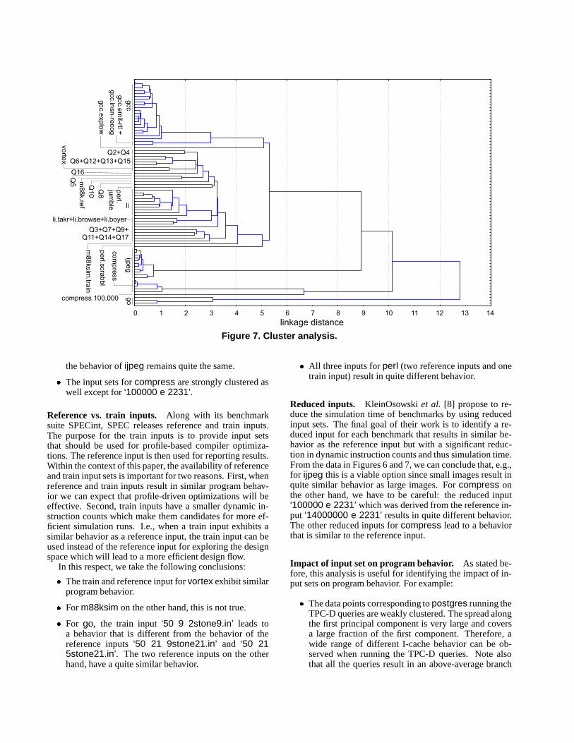
The results of the analyses that were done on these data,are shown in Figures 6 and 7. Figure 6 represents theprogram-input pairs in the 4-dimensional workload spacebuilt up by the four retained principal components. Thedendrogram corresponding to the cluster analysis is shownin Figure 7. Program-input pairs connected by small link-age distances are clustered in early iterations of the analysisand thus, exhibit ‘similar’ behavior. Program-input pairs onthe other hand, connected by large linkage distances exhibitdifferent behavior.
Isolated points. From the data presented in Figures 6and 7, it is clear that benchmarks go, ijpeg and compressare isolated in this 4-dimensional space. Indeed, in the den-drogram shown in Figure 7, these three benchmarks areconnected to the other benchmarks through long linkagedistances. E.g., go is connected to the other benchmarkswith a linkage distance of 12.8 which is much larger thanthe linkage distance for more strongly clustered pairs, e.g.,
2 or 4. An explanation for this phenomenon can be foundin Figure 6. Compress discriminates itself along the thirdcomponent which is due to its high D-cache miss rate. Forijpeg, the different behavior is due to, along the fourth com-ponent, the high percentage of arithmetic and shift opera-tions, the high number of instructions between two takenbranches and the low percentage of load/store and controloperations. For go the discrimination is made along the sec-ond component or the low branch prediction accuracy, thelow percentage of logical operations and the high amountof ILP.
Strong clusters. There are also several strong clusterswhich suggests that only a small number (or in some cases,only one) of the input sets should be selected to representthe whole cluster. This will ultimately reduce the total sim-ulation time since only a few (or only one) program-inputpairs need to be simulated instead of all the pairs within thatcluster. We can identify several strong clusters:�
The data points corresponding to the gcc benchmarkare strongly clustered, except for the input sets emit-rtl, insn-emit and explow. These three input sets ex-hibit a different behavior from the rest of the input sets.However, emit-rtl and insn-emit have a quite similarbehavior.�The data points corresponding to the lisp interpreter liexcept for browse, boyer and takr are strongly clus-tered as well. This can be clearly seen from Figure 7where this group is clustered with a linkage distancethat is smaller than 2. The three input sets with a dif-ferent behavior are grouped with the other li input setswith a linkage distance of approximately 3. The vari-ety within li is caused by the data cache miss rate mea-sured by the third principal component, see Figure 6.

-3
-2
-1
0
1
2
3
4
-2 -1 0 1 2 3
principal component 1
princip
alc
om
ponent2
-2.5
-1.5
-0.5
0.5
1.5
2.5
-2 -1 0 1 2 3 4
principal component 3
princip
alc
om
ponent4
Q17
gcc.emit-rtl
gcc.insn-emit
Q3
Q’svortex.train
vortex.ref
gcc.explowgccperl.scrabbl
m88ksim.ref
Q5
perl.jumble
perl.primes
m88ksim.train
ijpeg + li+ compress
go
ijpeg
compress
gcc.explow
compress.100,000
Q7
Q9
Q8
go.2stone9
m88ksim.train
perl.scrabbl
li.takr
li.browse
li.boyer
perl.primes
li.triang
li.destrum2
li.puzzle0
li
500,000
1,000,000
Q11
Q9Q7
Q2Q4
Q10
Q16
Q8
m88ksim.ref
Q’sQ11
perl.jumble
vortex.trainvortex.ref
gccgo
Figure 6. Workload space for all program-input pairs: first component vs. second component (uppergraph) and third vs. fourth component (bottom graph).
�According to Figure 7, there is also a small cluster con-taining TPC-D queries, namely queries 6, 12, 13 and15.�All input sets for ijpeg result in similar program behav-
ior since all input sets are clustered in one group. Animportant conclusion from this analysis is that in spiteof the differences in image dimensions, ranging fromsmall images (512x482) to large images (2362x1570),
0 2 4 6 8 10 12 14
com
pre
ss
linkage distance
go
gcc.e
mit-rtl +
gcc.in
sn
-reco
g
gcc
gcc.e
xp
low
Q6+Q12+Q13+Q15
vo
rtex
li
Q16Q5 m
88
k.re
f
Q1
0
Q8
pe
rl.ju
mb
le
Q3+Q7+Q9+Q11+Q14+Q17
m8
8ksim
.train
pe
rl.scra
bb
l
0 1 2 3 4 5 6 7 8 9 10 11 12 13 14
li.takr+li.browse+li.boyer
Q2+Q4
ijpe
g
compress.100,000
Figure 7. Cluster analysis.
the behavior of ijpeg remains quite the same.�The input sets for compress are strongly clustered aswell except for ‘100000 e 2231’.
Reference vs. train inputs. Along with its benchmarksuite SPECint, SPEC releases reference and train inputs.The purpose for the train inputs is to provide input setsthat should be used for profile-based compiler optimiza-tions. The reference input is then used for reporting results.Within the context of this paper, the availability of referenceand train input sets is important for two reasons. First, whenreference and train inputs result in similar program behav-ior we can expect that profile-driven optimizations will beeffective. Second, train inputs have a smaller dynamic in-struction counts which make them candidates for more ef-ficient simulation runs. I.e., when a train input exhibits asimilar behavior as a reference input, the train input can beused instead of the reference input for exploring the designspace which will lead to a more efficient design flow.
In this respect, we take the following conclusions:�The train and reference input for vortex exhibit similarprogram behavior.�For m88ksim on the other hand, this is not true.�For go, the train input ‘50 9 2stone9.in’ leads toa behavior that is different from the behavior of thereference inputs ‘50 21 9stone21.in’ and ‘50 215stone21.in’. The two reference inputs on the otherhand, have a quite similar behavior.
�All three inputs for perl (two reference inputs and onetrain input) result in quite different behavior.
Reduced inputs. KleinOsowski et al. [8] propose to re-duce the simulation time of benchmarks by using reducedinput sets. The final goal of their work is to identify a re-duced input for each benchmark that results in similar be-havior as the reference input but with a significant reduc-tion in dynamic instruction counts and thus simulation time.From the data in Figures 6 and 7, we can conclude that, e.g.,for ijpeg this is a viable option since small images result inquite similar behavior as large images. For compress onthe other hand, we have to be careful: the reduced input‘100000 e 2231’ which was derived from the reference in-put ‘14000000 e 2231’ results in quite different behavior.The other reduced inputs for compress lead to a behaviorthat is similar to the reference input.
Impact of input set on program behavior. As stated be-fore, this analysis is useful for identifying the impact of in-put sets on program behavior. For example:�
The data points corresponding to postgres running theTPC-D queries are weakly clustered. The spread alongthe first principal component is very large and coversa large fraction of the first component. Therefore, awide range of different I-cache behavior can be ob-served when running the TPC-D queries. Note alsothat all the queries result in an above-average branch

prediction accuracy, a high percentage of logical op-erations and low ILP (negative value along the secondprincipal component).�The difference in behavior between the input sets forcompress is mainly due to the difference in the datacache miss rates (along the third principal component).�In general, the variation between programs is largerthan the variation between input sets for the same pro-gram. Thus, when composing a workload, it is moreimportant to select different programs with a well cho-sen input set than to include various inputs for the sameprogram. For example, the program-input pairs forgcc (except for explow, emit-rtl and insn-emit) andijpeg are strongly clustered in the workload space. Insome cases however, for example postgres and perl,the input set has a relatively high impact on programbehavior.
4.3 Preliminary validation
As stated before, the purpose of the analysis presentedin this paper is to identify clusters of program-input pairsthat exhibit similar behavior. We will show that pairs thatare close to each other in the workload space indeed exhibitsimilar behavior when changes are made to the microarchi-tecture on which they run.
In this section, we present a preliminary validation inwhich we observe the behavior of several input sets for gccand one input set of each of the following benchmarks: goand li. The reason for doing a validation using a selectednumber of program-input pairs instead of all 79 program-input pairs is to limit simulation time. The simulations thatare presented in this section already took several weeks. Asa consequence, simulating all program-input pairs wouldhave been impractically long1. However, since gcc presentsa very diverse behavior (strong clustering versus isolatedpoints, see Figure 2), we believe that a succesful validationon gcc with some additional program-input pairs can be ex-trapolated to the complete workload space with confidence.
We have used seven input sets for gcc, namely explow,insn-recog, gcc, genoutput, stmt, insn-emit and emit-rtl. According to the analysis done in section 4.2.1, emit-rtland insn-emit should exhibit a similar behavior; the sameshould be true for gcc, genoutput and stmt. explow andinsn-recog on the other hand, should result in a differentprogram behavior since they are quite far away from theother input sets that are selected for this analysis. For goand li, we used 50 9 2stone9.in and boyer, respectively.
We used SimpleScalar v3.0 [2] for the Alpha architectureas simulation tool for this analysis. The baseline architec-ture has a window size of 64 instructions and an issue widthof 4.
In Figures 8, 9, 10 and 11, the number of instructions re-tired per cycle (IPC) is shown as a function of the I-cacheconfiguration, the D-cache configuration, the branch predic-tor and the window size versus issue width configuration,
1This is exactly the problem we are trying to solve.
1.1
1.2
1.3
1.4
1.5
1.6
1.7
1.8
1.9
8KB,
DM
16KB,
DM
16KB,
2WSA
32KB,
DM
32KB,
2WSA
32KB,
4WSA
Instruction Cache
IPC
explow
insn-recog
gcc
genoutput
stmt
insn-emit
emit-rtl
go
li
Figure 8. IPC as a function of the I-cache con-figuration; 16KB DM D-cache and 8K-entry bi-modal branch predictor.
1.3
1.4
1.5
1.6
1.7
1.8
1.9
8KB,
DM
16KB,
DM
16KB,
2WSA
32KB,
DM
32KB,
2WSA
32KB,
4WSA
Data Cache
IPC
explow
insn-recog
gcc
genoutput
stmt
insn-emit
emit-rtl
go
li
Figure 9. IPC as a function of the D-cacheconfiguration; 32KB DM I-cache and 8K-entrybimodal branch predictor.
respectively. We will first discuss the results for gcc. After-wards, we will detail on the other benchmarks.
For gcc, we clearly identify three groups of input setsthat have similar behavior, namely (i) explow and insn-recog, (ii) gcc, genoutput and stmt, and (iii) insn-emitand emit-rtl. For example, in Figure 10, the branch behav-ior of group (i) is significantly different from the other inputsets. Or, in Figure 11, the scaling behavior as a function ofwindow size and issue width is quite different for all threegroups. This could be expected for groups (ii) and (iii) asdiscussed earlier. The fact that explow and insn-recog ex-hibit similar behavior on the other hand, is unexpected sincethese two input sets are quite far away from each other in theworkload space, see Figure 2. The discrimination betweenthese two input sets is primarily along the second compo-
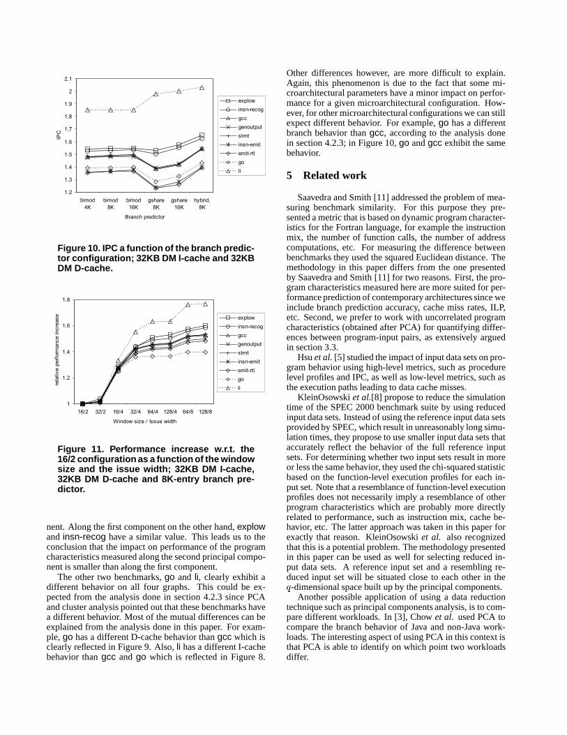
1.2
1.3
1.4
1.5
1.6
1.7
1.8
1.9
2
2.1
bimod
4K
bimod
8K
bimod
16K
gshare
8K
gshare
16K
hybrid,
8K
Branch predictor
IPC
explow
insn-recog
gcc
genoutput
stmt
insn-emit
emit-rtl
go
li
Figure 10. IPC a function of the branch predic-tor configuration; 32KB DM I-cache and 32KBDM D-cache.
1
1.2
1.4
1.6
1.8
16/2 32/2 16/4 32/4 64/4 128/4 64/8 128/8
Window size / Issue width
rela
tive
perf
orm
ance
incre
ase explow
insn-recog
gcc
genoutput
stmt
insn-emit
emit-rtl
go
li
Figure 11. Performance increase w.r.t. the16/2 configuration as a function of the windowsize and the issue width; 32KB DM I-cache,32KB DM D-cache and 8K-entry branch pre-dictor.
nent. Along the first component on the other hand, explowand insn-recog have a similar value. This leads us to theconclusion that the impact on performance of the programcharacteristics measured along the second principal compo-nent is smaller than along the first component.
The other two benchmarks, go and li, clearly exhibit adifferent behavior on all four graphs. This could be ex-pected from the analysis done in section 4.2.3 since PCAand cluster analysis pointed out that these benchmarks havea different behavior. Most of the mutual differences can beexplained from the analysis done in this paper. For exam-ple, go has a different D-cache behavior than gcc which isclearly reflected in Figure 9. Also, li has a different I-cachebehavior than gcc and go which is reflected in Figure 8.
Other differences however, are more difficult to explain.Again, this phenomenon is due to the fact that some mi-croarchitectural parameters have a minor impact on perfor-mance for a given microarchitectural configuration. How-ever, for other microarchitectural configurations we can stillexpect different behavior. For example, go has a differentbranch behavior than gcc, according to the analysis donein section 4.2.3; in Figure 10, go and gcc exhibit the samebehavior.
5 Related work
Saavedra and Smith [11] addressed the problem of mea-suring benchmark similarity. For this purpose they pre-sented a metric that is based on dynamic program character-istics for the Fortran language, for example the instructionmix, the number of function calls, the number of addresscomputations, etc. For measuring the difference betweenbenchmarks they used the squared Euclidean distance. Themethodology in this paper differs from the one presentedby Saavedra and Smith [11] for two reasons. First, the pro-gram characteristics measured here are more suited for per-formance prediction of contemporary architectures since weinclude branch prediction accuracy, cache miss rates, ILP,etc. Second, we prefer to work with uncorrelated programcharacteristics (obtained after PCA) for quantifying differ-ences between program-input pairs, as extensively arguedin section 3.3.
Hsu et al. [5] studied the impact of input data sets on pro-gram behavior using high-level metrics, such as procedurelevel profiles and IPC, as well as low-level metrics, such asthe execution paths leading to data cache misses.
KleinOsowski et al.[8] propose to reduce the simulationtime of the SPEC 2000 benchmark suite by using reducedinput data sets. Instead of using the reference input data setsprovided by SPEC, which result in unreasonably long simu-lation times, they propose to use smaller input data sets thataccurately reflect the behavior of the full reference inputsets. For determining whether two input sets result in moreor less the same behavior, they used the chi-squared statisticbased on the function-level execution profiles for each in-put set. Note that a resemblance of function-level executionprofiles does not necessarily imply a resemblance of otherprogram characteristics which are probably more directlyrelated to performance, such as instruction mix, cache be-havior, etc. The latter approach was taken in this paper forexactly that reason. KleinOsowski et al. also recognizedthat this is a potential problem. The methodology presentedin this paper can be used as well for selecting reduced in-put data sets. A reference input set and a resembling re-duced input set will be situated close to each other in the� -dimensional space built up by the principal components.
Another possible application of using a data reductiontechnique such as principal components analysis, is to com-pare different workloads. In [3], Chow et al. used PCA tocompare the branch behavior of Java and non-Java work-loads. The interesting aspect of using PCA in this context isthat PCA is able to identify on which point two workloadsdiffer.

Huang and Shen [6] evaluated the impact of input datasets on the bandwidth requirements of computer programs.
Changes in program behavior due to different input datasets are also important for profile-guided compilation [12],where profiling information from a past run is used by thecompiler to guide its optimisations. Fisher and Freuden-berger [4] studied whether branch directions from previ-ous runs of a program (using different input sets) are goodpredictors of the branch directions in future runs. Theirstudy concludes that branches generally take the same di-rections in different runs of a program. However, theywarn that some runs of a program exercise entirely differ-ent parts of the program. Hence, these runs cannot be usedto make predictions about each other. By using the aver-age branch direction over a number of runs, this problemcan be avoided. Wall [15] studied several types of profilessuch as basic block counts and the number of references toglobal variables. He measured the usefulness of a profile asthe speedup obtained when that profile is used in a profile-guided compiler optimisation. Seemingly, the best resultsare obtained when the same input is used for profiling andmeasuring the speedup. This implies that every input is dif-ferent in some sense and leads to different compiler optimi-sations.
6 Conclusion
In microprocessor design, it is important to have a repre-sentative workload to make correct design decisions. Thispaper proposes the use of principal components analysisand cluster analysis to efficiently explore the workloadspace. In this workload space, benchmark-input pairs canbe displayed and a distance can be computed that gives us anidea of the behavioral difference between these benchmark-input pairs. This representation can be used to measure theimpact of input data sets on program behavior. In addition,our methodology was succesfully validated by showing thatprogram-input pairs that are close to each other in the prin-cipal components space, indeed exhibit similar behavior asa function of microarchitectural changes. Interesting appli-cations for this technique are the composition of workloadsand profile-based compiler optimizations.
Acknowledgements
Lieven Eeckhout and Hans Vandierendonck are sup-ported by a grant from the Flemish Institute for the Promo-tion of the Scientific-Technological Research in the Industry(IWT). The authors would also like to thank the anonymousreviewers for their valuable comments.
References
[1] P. Bose and T. M. Conte. Performance analysis and its impacton design. IEEE Computer, 31(5):41–49, May 1998.
[2] D. C. Burger and T. M. Austin. The SimpleScalar ToolSet. Computer Architecture News, 1997. Version 2.0. See
also http://www.simplescalar.org for more infor-mation.
[3] K. Chow, A. Wright, and K. Lai. Characterization of Javaworkloads by principal components analysis and indirectbranches. In Proceedings of the Workshop on Workload Char-acterization (WWC-1998), held in conjunction with the 31stAnnual ACM/IEEE International Symposium on Microarchi-tecture (MICRO-31), pages 11–19, Nov. 1998.
[4] J. Fisher and S. Freudenberger. Predicting conditional branchdirections from previous runs of a program. In Proc. of theFifth International Conference on Architectural Support forProgramming Languages and Operating Systems (ASPLOS-V), pages 85–95, 1992.
[5] W. C. Hsu, H. Chen, P. Y. Yew, and D.-Y. Chen. On the pre-dictability of program behavior using different input data sets.In Proceedings of the Sixth Workshop on Interaction betweenCompilers and Computer Architectures (INTERACT 2002),held in conjunction with the Eighth International Sympo-sium on High-Performance Computer Architecture (HPCA-8), pages 45–53, Feb. 2002.
[6] A. S. Huang and J. P. Shen. The intrinsic bandwidth require-ments of ordinary programs. In Proceedings of the SeventhInternational Conference on Architectural Support for Pro-gramming Languages and Operating Systems (ASPLOS-VII),pages 105–114, Oct. 1996.
[7] L. K. John, P. Vasudevan, and J. Sabarinathan. Workload char-acterization: Motivation, goals and methodology. In L. K.John and A. M. G. Maynard, editors, Workload Characteriza-tion: Methodology and Case Studies. IEEE Computer Soci-ety, 1999.
[8] A. J. KleinOsowski, J. Flynn, N. Meares, and D. J. Lilja.Adapting the SPEC 2000 benchmark suite for simulation-based computer architecture research. In Workload Charac-terization of Emerging Computer Applications, Proceedingsof the IEEE 3rd Annual Workshop on Workload Character-ization (WWC-2000) held in conjunction with the Interna-tional Conference on Computer Design (ICCD-2000), pages83–100, Sept. 2000.
[9] B. F. J. Manly. Multivariate Statistical Methods: A primer.Chapman & Hall, second edition, 1994.
[10] S. McFarling. Combining branch predictors. Technical Re-port WRL TN-36, Digital Western Research Laboratory, June1993.
[11] R. H. Saavedra and A. J. Smith. Analysis of benchmarkcharacteristics and benchmark performance prediction. ACMTransactions on Computer Systems, 14(4):344–384, Nov.1996.
[12] M. D. Smith. Overcoming the challenges to feedback-directed optimization (keynote talk). In Proceedings of ACMSIGPLAN Workshop on Dynamic and Adaptive Compilationand Optimization, pages 1–11, 2000.
[13] A. Srivastava and A. Eustace. ATOM: A system for buildingcustomized program analysis tools. Technical Report 94/2,Western Research Lab, Compaq, Mar. 1994.
[14] I. StatSoft. STATISTICA for Windows. Computer programmanual. 1999. http://www.statsoft.com.
[15] D. W. Wall. Predicting program behavior using real or esti-mated profiles. In Proceedings of the 1991 International Con-ference on Programming Language Design and Implementa-tion (PLDI-1991), pages 59–70, 1991.