WORKSHOP 13

NORMAL MODES OF A RECTANGULAR PLATE

WS13-2NAS120, Workshop 13, May 2006Copyright© 2005 MSC.Software Corporation

WS13-3NAS120, Workshop 13, May 2006Copyright© 2005 MSC.Software Corporation

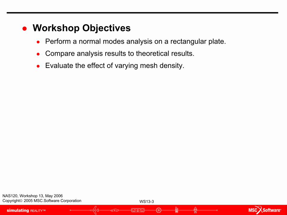
Workshop ObjectivesPerform a normal modes analysis on a rectangular plate.

Compare analysis results to theoretical results.

Evaluate the effect of varying mesh density.

WS13-4NAS120, Workshop 13, May 2006Copyright© 2005 MSC.Software Corporation

Problem DescriptionA rectangular plate is simply supported at all edges. Find the first 10 normal modes for this plate. E = 10 x 106 psiν =0.33ρ = 0.101 lb/in3

t = 0.125 in

WS13-5NAS120, Workshop 13, May 2006Copyright© 2005 MSC.Software Corporation

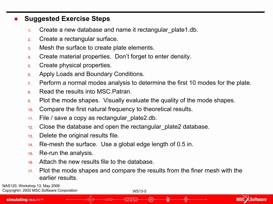
Suggested Exercise Steps1. Create a new database and name it rectangular_plate1.db. 2. Create a rectangular surface.3. Mesh the surface to create plate elements. 4. Create material properties. Don’t forget to enter density.5. Create physical properties.6. Apply Loads and Boundary Conditions.7. Perform a normal modes analysis to determine the first 10 modes for the plate.8. Read the results into MSC.Patran.9. Plot the mode shapes. Visually evaluate the quality of the mode shapes. 10. Compare the first natural frequency to theoretical results. 11. File / save a copy as rectangular_plate2.db.12. Close the database and open the rectangular_plate2 database.13. Delete the original results file.14. Re-mesh the surface. Use a global edge length of 0.5 in.15. Re-run the analysis.16. Attach the new results file to the database.17. Plot the mode shapes and compare the results from the finer mesh with the

earlier results.

WS13-6NAS120, Workshop 13, May 2006Copyright© 2005 MSC.Software Corporation

b c

d

f

g

Step 1. Create New Database

Create a new database called rectangular_plate1.db

a. File / New.b. Enter

rectangular_plate1 as the file name.

c. Click OK.d. Choose Default

Tolerance.e. Select MSC.Nastran as

the Analysis Code.f. Select Structural as the

Analysis Type. g. Click OK.

a

e

WS13-7NAS120, Workshop 13, May 2006Copyright© 2005 MSC.Software Corporation

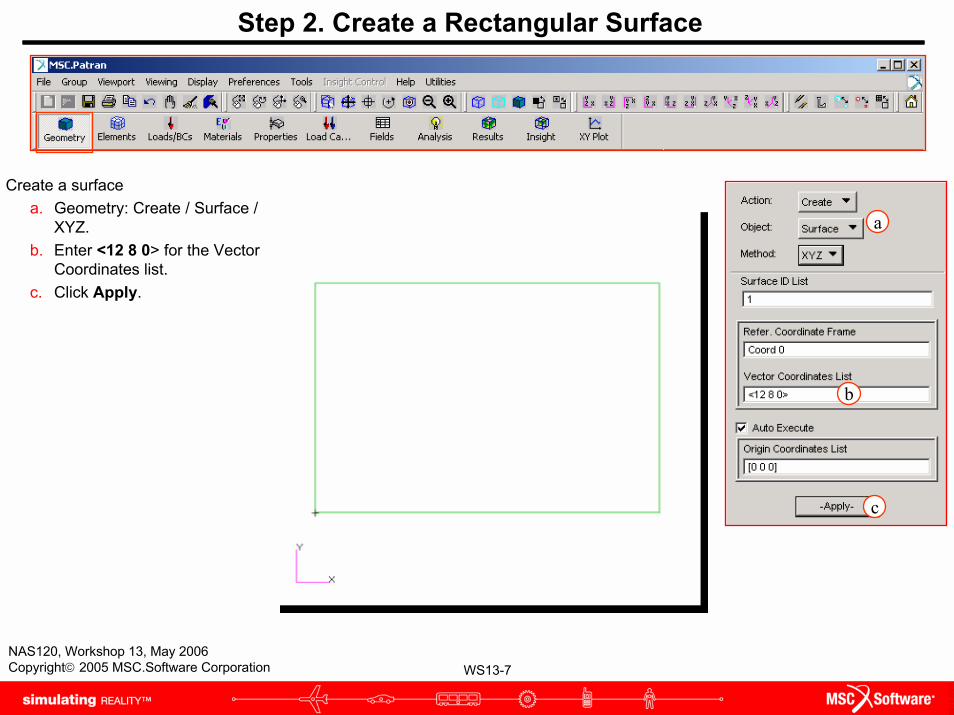
Step 2. Create a Rectangular Surface

Create a surfacea. Geometry: Create / Surface /

XYZ.b. Enter <12 8 0> for the Vector

Coordinates list.c. Click Apply.

b

c

a

WS13-8NAS120, Workshop 13, May 2006Copyright© 2005 MSC.Software Corporation

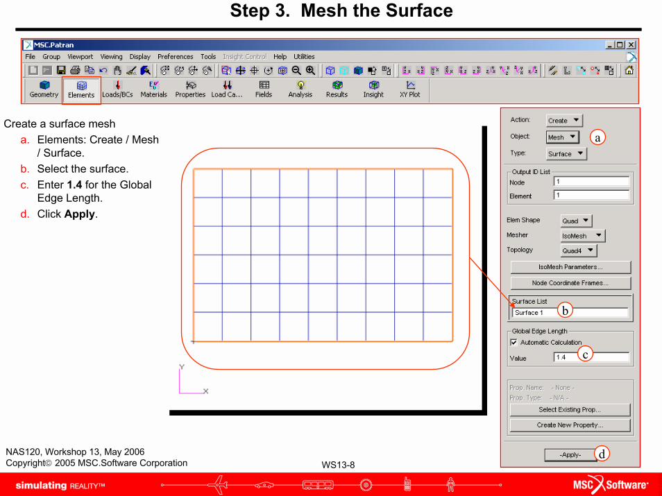
Step 3. Mesh the Surface

Create a surface mesha. Elements: Create / Mesh

/ Surface.b. Select the surface.c. Enter 1.4 for the Global

Edge Length.d. Click Apply.

a

b

c

d

WS13-9NAS120, Workshop 13, May 2006Copyright© 2005 MSC.Software Corporation

Step 4. Create Material Properties

Create an isotropic materiala. Materials: Create / Isotropic

/ Manual Input.b. Enter plate_material for

the Material Name.c. Click Input Properties.d. Enter 10e6 for the Elastic

Modulus.e. Enter 0.33 for the Poisson

Ratio.f. Enter 0.101 for the Density.g. Click OK. h. Click Apply.

d

g

e

f

a

c

b

h

WS13-10NAS120, Workshop 13, May 2006Copyright© 2005 MSC.Software Corporation

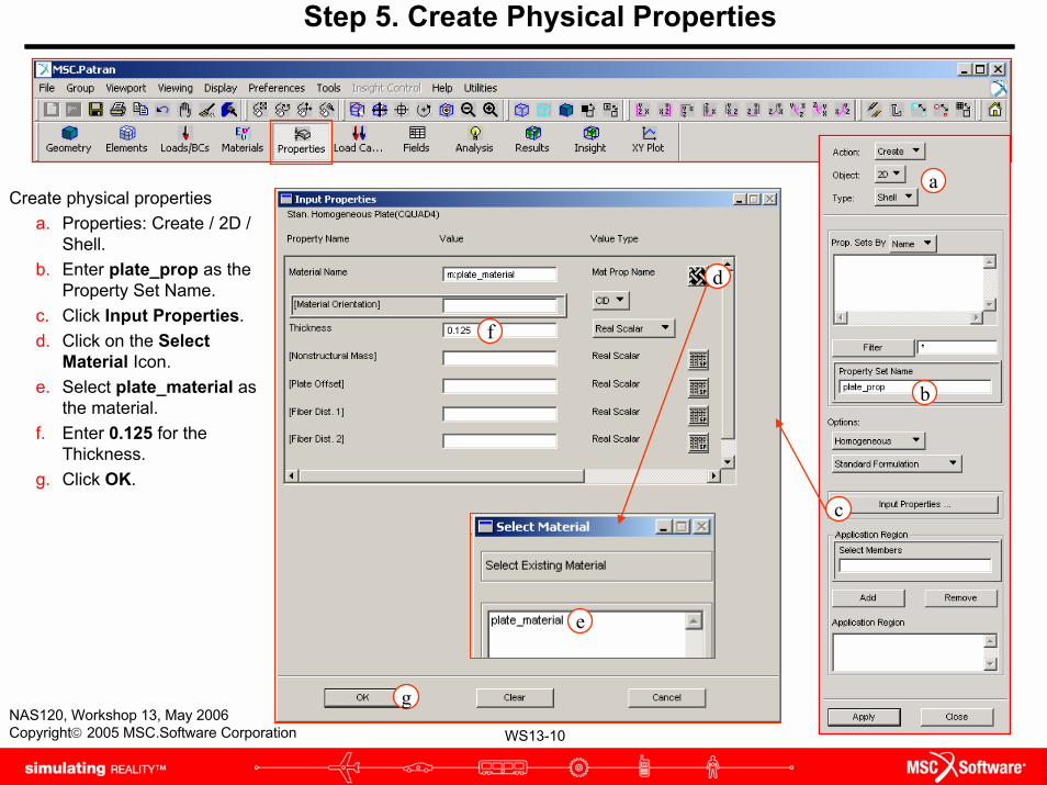
Step 5. Create Physical Properties

Create physical propertiesa. Properties: Create / 2D /

Shell.b. Enter plate_prop as the

Property Set Name.c. Click Input Properties.d. Click on the Select

Material Icon.e. Select plate_material as

the material.f. Enter 0.125 for the

Thickness.g. Click OK.

g

d

f

e

a

b

c

WS13-11NAS120, Workshop 13, May 2006Copyright© 2005 MSC.Software Corporation

Apply the physical propertiesa. Click in the Select

Members box.b. Screen pick the plate

as shown.c. Click Add.d. Click Apply.

b

Step 5. Create Physical Properties

a

c

d

WS13-12NAS120, Workshop 13, May 2006Copyright© 2005 MSC.Software Corporation

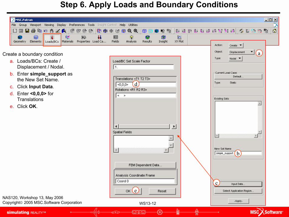
Step 6. Apply Loads and Boundary Conditions

Create a boundary conditiona. Loads/BCs: Create /

Displacement / Nodal.b. Enter simple_support as

the New Set Name.c. Click Input Data.d. Enter <0,0,0> for

Translations e. Click OK.

d

e

b

c

a

WS13-13NAS120, Workshop 13, May 2006Copyright© 2005 MSC.Software Corporation

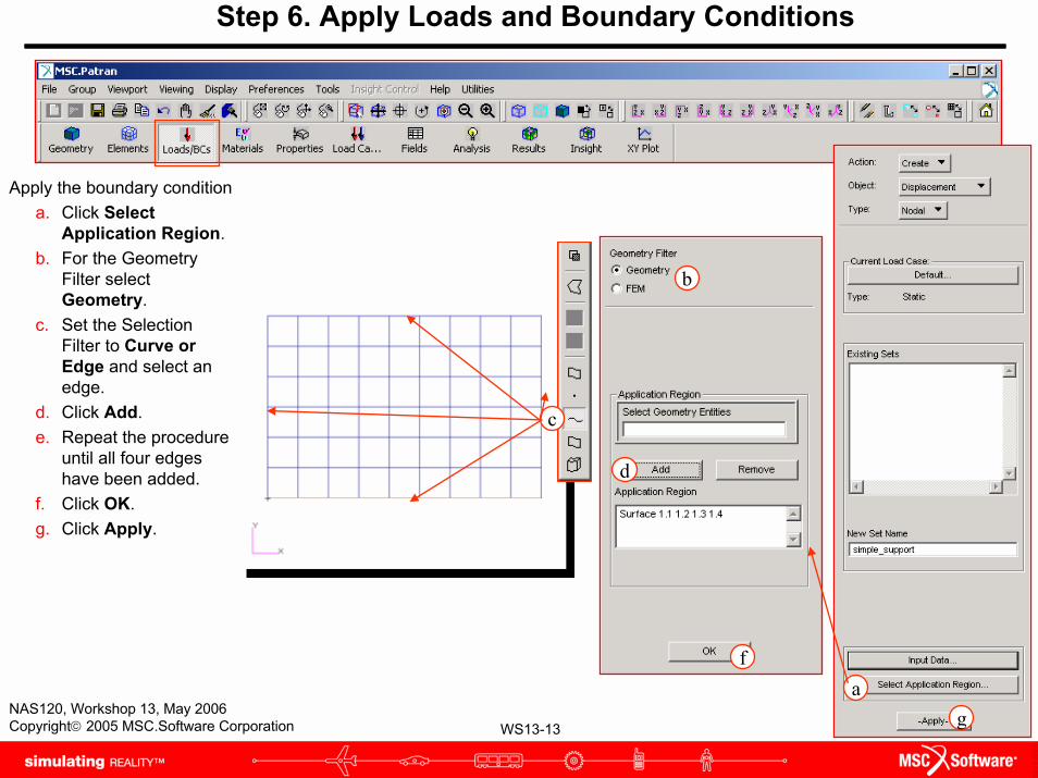
Apply the boundary conditiona. Click Select

Application Region.b. For the Geometry

Filter select Geometry.

c. Set the Selection Filter to Curve or Edge and select an edge.

d. Click Add.e. Repeat the procedure

until all four edges have been added.

f. Click OK. g. Click Apply.

f

d

b

Step 6. Apply Loads and Boundary Conditions

c

ag

WS13-14NAS120, Workshop 13, May 2006Copyright© 2005 MSC.Software Corporation

Step 7. Run Normal Modes Analysis

Analyze the modela. Analysis: Analyze / Entire

Model / Full Run.b. Click Solution Type.c. Choose Normal Modes.d. Click Solution Parameters.e. Enter 0.00259 for Wt.-Mass

conversion.f. Click OK.g. Click OK. h. Click Apply.

c

gf

e

d

a

h

b

WS13-15NAS120, Workshop 13, May 2006Copyright© 2005 MSC.Software Corporation

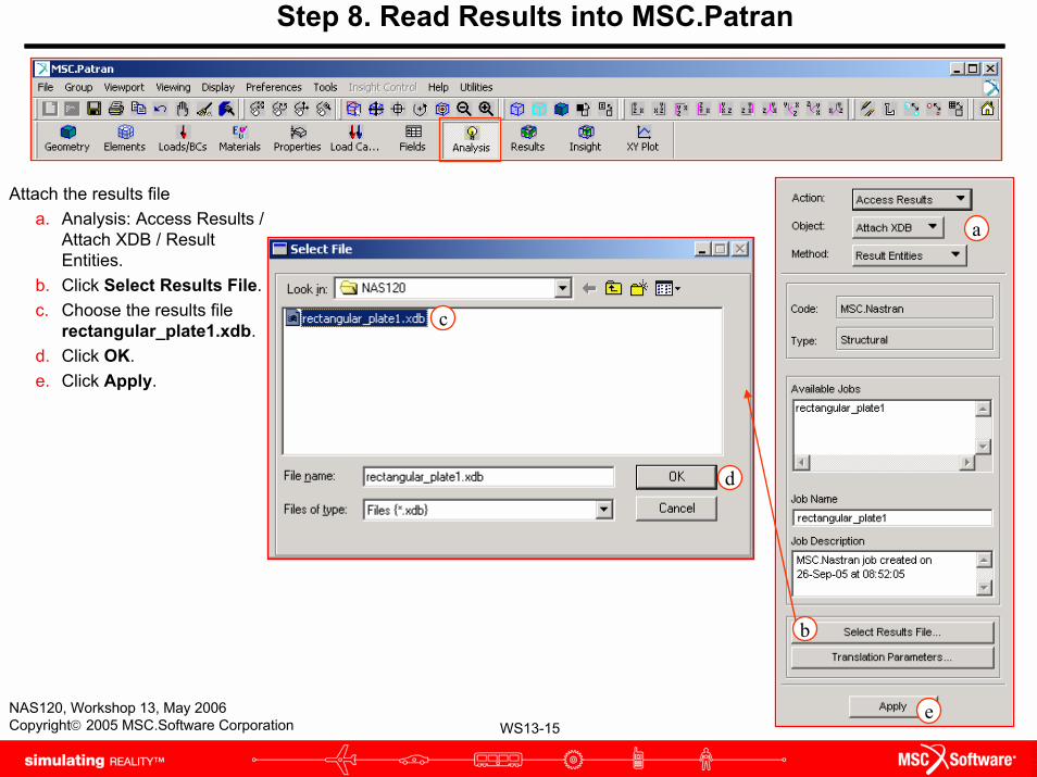
Step 8. Read Results into MSC.Patran

Attach the results filea. Analysis: Access Results /

Attach XDB / Result Entities.

b. Click Select Results File.c. Choose the results file

rectangular_plate1.xdb.d. Click OK. e. Click Apply.

a

b

c

e

d

WS13-16NAS120, Workshop 13, May 2006Copyright© 2005 MSC.Software Corporation

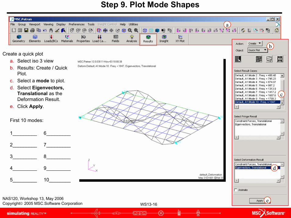
Step 9. Plot Mode Shapes

Create a quick plota. Select iso 3 viewb. Results: Create / Quick

Plot.c. Select a mode to plot.d. Select Eigenvectors,

Translational as the Deformation Result.

e. Click Apply.

First 10 modes:

1_________ 6_________

2_________ 7_________

3_________ 8_________

4_________ 9_________

5_________ 10________

b

e

d

a

c

WS13-17NAS120, Workshop 13, May 2006Copyright© 2005 MSC.Software Corporation

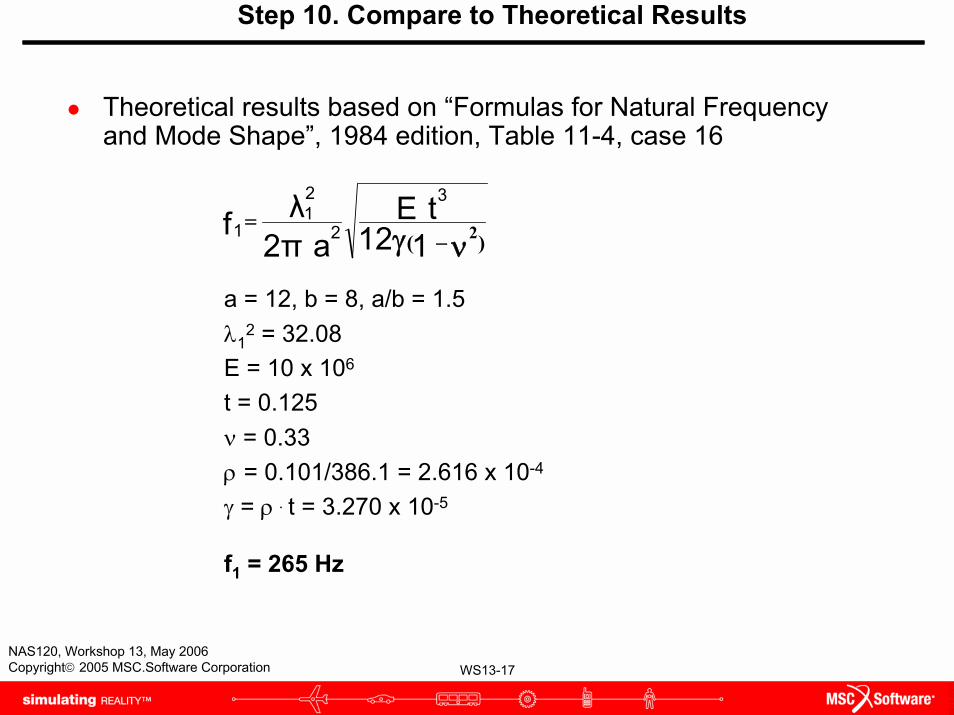
Step 10. Compare to Theoretical Results

Theoretical results based on “Formulas for Natural Frequency and Mode Shape”, 1984 edition, Table 11-4, case 16

)( 2νγ −=

112tE

a2πλf

3

2

21

1

a = 12, b = 8, a/b = 1.5λ1

2 = 32.08E = 10 x 106

t = 0.125ν = 0.33ρ = 0.101/386.1 = 2.616 x 10-4

γ = ρ . t = 3.270 x 10-5

f1 = 265 Hz

WS13-18NAS120, Workshop 13, May 2006Copyright© 2005 MSC.Software Corporation

Step 11. Save a Copy

Save a copy of the filea. File: Save a Copy.b. Type rectangular_plate2

as the file name.c. Click Save.

a

b c

WS13-19NAS120, Workshop 13, May 2006Copyright© 2005 MSC.Software Corporation

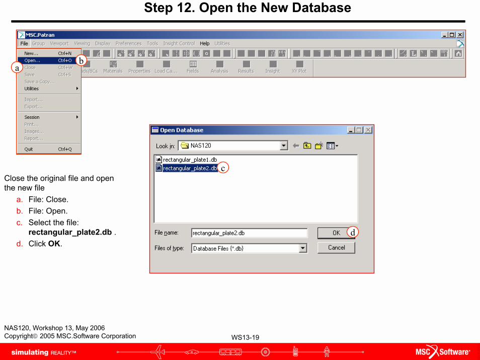
Step 12. Open the New Database

Close the original file and open the new file

a. File: Close.b. File: Open.c. Select the file:

rectangular_plate2.db .d. Click OK.

ab

c

d

WS13-20NAS120, Workshop 13, May 2006Copyright© 2005 MSC.Software Corporation

Step 13. Delete Old Results File

Delete XDB attachmenta. Analysis: Delete / XDB

Attachment.b. Select the

rectangular_plate1 .xdb attachment.

c. Click Apply.d. Choose Yes to delete

the attachment.e. Click on the front view

icon.

a

b

c

e

d

WS13-21NAS120, Workshop 13, May 2006Copyright© 2005 MSC.Software Corporation

Step 14. Re-Mesh the Surface

Create a finer mesha. Elements: Create / Mesh

/ Surface.b. Select the entire surface.c. Enter 0.5 for the Global

Edge Length.d. Click Apply.e. Choose Yes to delete

the existing mesh.

e

a

b

c

d

WS13-22NAS120, Workshop 13, May 2006Copyright© 2005 MSC.Software Corporation

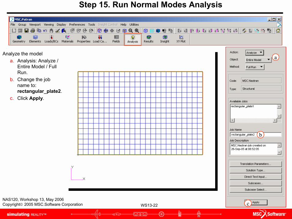
Step 15. Run Normal Modes Analysis

Analyze the modela. Analysis: Analyze /

Entire Model / Full Run.

b. Change the job name to: rectangular_plate2.

c. Click Apply.

a

b

c

WS13-23NAS120, Workshop 13, May 2006Copyright© 2005 MSC.Software Corporation

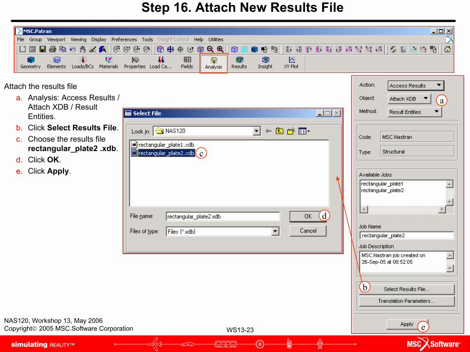
Step 16. Attach New Results File

Attach the results filea. Analysis: Access Results /

Attach XDB / Result Entities.

b. Click Select Results File.c. Choose the results file

rectangular_plate2 .xdb.d. Click OK. e. Click Apply.

a

b

c

e

d

WS13-24NAS120, Workshop 13, May 2006Copyright© 2005 MSC.Software Corporation

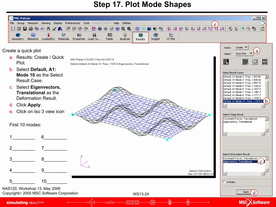
Step 17. Plot Mode Shapes

Create a quick plota. Results: Create / Quick

Plot.b. Select Default, A1:

Mode 10 as the Select Result Case.

c. Select Eigenvectors, Translational as the Deformation Result.

d. Click Apply.e. Click on Iso 3 view icon

First 10 modes:

1_________ 6_________

2_________ 7_________

3_________ 8_________

4_________ 9_________

5_________ 10________

a

d

c

e

b