The Second KDD Workshop on

Mining Multiple Information Sources

MMIS′08 Held in conjunction with the 14th ACM SIGKDD

International Conference, August 24, 2008

Las Vegas, Nevada, USA

Workshop Co-Chairs Xingquan Zhu Ruoming Jin Yuri Breitbart

ISBN: 978-1-60558-273-3

The Association for Computing Machinery, Inc. 1515 Broadway

New York, New York 10036

Copyright © 2008 by the Association for Computing Machinery, Inc (ACM). Permission to make digital or hard copies of portions of this work for personal or classroom use is granted without fee provided that the copies are not made or distributed for profit or commercial advantage and that copies bear this notice and the full citation on the first page. Copyrights for components of this work owned by others than ACM must be honored. Abstracting with credit is permitted. To copy otherwise, to republish, to post on servers or to redistribute to lists, requires prior specific permission and/or a fee. Request permission to republish from: Publications Dept. ACM, Inc. Fax +1-212-869-0481 or E-mail permissions@acm.org. For other copying of articles that carry a code at the bottom of the first or last page, copying is permitted provided that the per-copy fee indicated in the code is paid through the Copyright Clearance Center, 222 Rosewood Drive, Danvers, MA 01923. Notice to Past Authors of ACM-Published Articles

ACM intends to create a complete electronic archive of all articles and/or other material previously published by ACM. If you have written a work that was previously published by ACM in any journal or conference proceedings prior to 1978, or any SIG Newsletter at any time, and you do NOT want this work to appear in the ACM Digital Library, please inform permissions@acm.org, stating the title of the work, the author(s), and where and when published.

ISBN: 978-1-60558-273-3

Additional copies may be ordered prepaid from

ACM Order Department Phone: 1-800-342-6626 P.O. BOX 11405 (U.S.A. and Canada) Church Street Station +1-212-626-0500 New York, NY 10286-1405 (All other countries)

Fax: +1-212-944-1318 E-mail: acmhelp@acm.org

2

Preface

As data collection sources and channels continuous evolve, mining and correlating information from multiple information sources has become a crucial step in data mining and knowledge discovery. On one hand, comparing patterns from different databases and understanding their relationships can be extremely beneficial for applications such as Bioinformatics, Sensor Networking, and Business Intelligence. In particular, important information such as pattern trends and evolving rules buried in each individual database, are very hard to discover by examining a single dataset only whereas comparatively mining multiple databases will enable users to discover interesting patterns across a set of data collections that would not have been possible otherwise. On the other hand, many data mining and data analysis tasks such as classification, regression, and clustering, can significantly improve their performance if information from different sources can be properly leveraged and if the mining process has the power to survey all the data sources involved.

Unleashing the full power of multiple information sources is, however, a very challenging problem, considering that schemas used to represent each data collections might be different (data heterogeneousity), data distributions and patterns underlying different data sources may undergo continuous changes (concept evolving), and mining tasks for each data source might also be different (mining diversity). Even though existing researches have demonstrated several approaches to utilize multiple information sources, these methods are still rather ad-hoc and inadequately address some of the fundamental research issues in this field: (1) Harnessing Complex Data Relationship: Multiple information sources represent a collection of highly correlated data, issues such as data integration, data integration, model integration, and model transferring across different domains, play fundamental roles in supporting KDD from multiple information sources; (2) Integrative and Cooperative Mining: For heterogeneous information sources with diverse mining tasks, the mining should be able to unify all data to generate enhanced global models, as well as help individual data collections to cooperatively achieve their respective mining goals; and (3) Differentiation and Correlation: Differentiate and coordinate the difference between data sources at the knowledge level is one crucial step for users to gain a high-level understanding of their data.

The aim of this workshop is to bring together data mining experts to revisit the problem of pattern discovery from multiple information sources, and identify and synthesize current needs for such purposes. Representative questions to be addressed include but are not limited to:

1. Harnessing Complex Data Relationship a. Database similarity assessment b. Automatic schema mapping and relationship discovery c. New mapping framework for multiple information sources d. Data source classification and clustering e. Data cleansing, data preparation, data/pattern selection, conflict and inconsistency

resolution 2. Integrative and Cooperative Mining

a. Model integration for heterogeneous information sources b. Mode transferring across different data domains c. Incremental and scalable data mining algorithms d. Multi-tasks multi-sources co-learning for multiple information sources

3. Differentiation and Correlation a. Local pattern analysis and fusion b. Global pattern synthesizing and assessment

3

c. Merging local rules for global pattern discovery d. Pattern summarization from multiple datasets e. Multi-dimensional pattern search and comparison f. Pattern comparison across multiple data sources g. Inter pattern discovery from complex data sources

4. Stream data mining algorithms a. Clustering and classification of data of changing distributions b. Data stream processing, storage, and retrieval systems c. Sensor networking

5. Security and privacy issues in multiple information sources 6. Interactive data mining systems

a. Query languages for mining multiple information sources b. Query optimization for distributed data mining c. Distributed data mining operators in supporting interactive data mining queries

In this proceedings, we include two keynote speaks and 6 papers selected from the submissions. We are grateful to all program committee members for their constructive comments and suggestions in organizing the workshop. We thank them for finishing all the reviews in a very short amount of time. We would also like to thank all the authors who submitted their papers to the workshop; we could not make an excellent workshop program without their support. The support of the National Science Foundation of China (#60674109) is acknowledged! More information about the workshop can be found at: http://www.cse.fau.edu/~xqzhu/mmis/kdd08_mmis.html August 2008

Xingquan Zhu

Ruoming Jin

Yuri Breitbart

4

MMIS′08 Workshop Organizing and Program Committee

Workshop Co-Chairs:

Xingquan Zhu Florida Atlantic University, USA

Ruoming Jin Kent State University, USA

Yuri Breitbart Kent State University, USA

Program Committee:

Walid G. Aref Purdue University, USA

Philip Chan Florida Institute of Technology, USA

Dejing Dou University of Oregon, USA

Christopher Jermaine University of Florida, USA

Taghi Khoshgoftaar Florida Atlantic University, USA

Tao Li Florida International University, USA

Huan Liu Arizona State University, USA

Prem Melville IBM T.J. Watson, USA

Jieping Ye Arizona State University, USA

Xintao Wu UNC Charlotte, USA

Shichao Zhang University of Technology, Sydney

Aoying Zhou Fudan University, China

Zhi-hua Zhou Nanjing University, China

5

Table of Contents

Keynote Speak • Harnessing Multiple Information Sources using Compositional Data Mining …7

Naren Ramakrishnan, Virginia Tech, USA

• Load Shedding in Stream Processing ………………………………………………… 8 Haixun Wang, IBM Thomas J. Watson Research Center, USA

List of Workshop Papers

• Signalling Potential Adverse Drug Reactions from Multiple Administrative Health Databases…………………………………………………………………………. 9 Huidong Jin1,2, Jie Chen1,3, Hongxing He1, Chris Kelman4, Damien McAullay1, Christine M. O’Keefe5 1 CSIRO Mathematical and Information Sciences, Australia 2 NICTA Canberra Laboratory, Australia 3 SigNav Pty Ltd, Australia 4 NCEPH, the Australian National University, Australia 5 CSIRO Preventative Health National Research Flagship, Australia

• An Exploration of Understanding Heterogeneity through Data Mining ……….. 18 Haishan Liu, Dejing Dou Dept. of Computer and Information Science, University of Oregon, USA

• Multiclass Multifeature Split Decision Tree Construction in a Distributed Environment …………………………………………………………………………… . 26 Jie Ouyang, Nilesh Patel, Ishwar Sethi Dept. of Computer Science and Engineering, Oakland University, USA

• A Novel Approach for Discovering Chain-Store High Utility Patterns in a Multi-Stores Environment………………………………………………………………………33 Guo-Cheng Lan, Vincent S. Tseng Dept. of Computer Science and Information Eng., National Cheng Kung University, Taiwan

• Large Scale Security Log Sources Integration: An Ensemble Method……………39 Jiajia Mao, Yan Wen, Aiping Li, Yan Jia, Quanyuan Wu School of Computer, National University of Defense Technology, China

• Applying MDA to Integrate Mining Techniques into Data Warehouses: A Time Series Case Study…………………………………………………………………………47 Jesús Pardillo1, Jose-Norberto Mazón1, Jose Zubcoff2, Juan Trujillo1 1Dept. of Software and Computing Systems, University of Alicante, Span 2Dept. of Sea Sciences and Applied Biology, University of Alicante, Span

6

Keynote Speak

Harnessing Multiple Information Sources using Compositional Data Mining

Dr. Naren Ramakrishnan, Virginia Tech, USA

Bioinformatics and biological data mining is essentially a cottage industry today: as new categories of data and information become available, scientists identify new ways to 'chain' inferences across them. Different scientists bring different perspectives and hence a survey of biological data mining algorithms today will resemble a 'solution first' landscape of specialized applications. To further advance data mining, what is needed is a compositional approach to building complex data mining applications from simple algorithms. This will enable us to capture complex patterns as compositions of simpler patterns. In this talk, we present such an approach using two basic pattern classes: redescriptions and biclusters. Whereas redescriptions identify patterns within a domain, biclusters identify patterns across domains. Both of them mirror shifts-of-vocabulary that can be functionally cascaded in arbitrary ways to create rich chains of inferences. Given a relational database and its schema,we show how the schema can be automatically compiled into a compositional data mining program, and how compositional patterns can be efficiently computed without 'wasteful' data mining. Several applications will be described. The end-goal is to bring the same 'building block' emphasis to data mining multiple sources that languages like SQL bring to querying.

7

Keynote Speak

Load Shedding in Stream Process

Dr. Haixun Wang, IBM Thomas J. Watson Research Center, USA

We consider the problem of resource allocation in mining multiple data streams. Due to the large volume and the high speed of streaming data, mining algorithms must cope with the effects of system overload. How to realize maximum mining benefits under resource constraints becomes a challenging task. In this paper, we propose a load shedding scheme for classifying multiple data streams. We focus on the following problems: i) how to classify data that are dropped by the load shedding scheme? and ii) how to decide when to drop data from a stream? We introduce a quality of decision (QoD) metric to measure the level of uncertainty in classification when exact feature values of the data are not available because of load shedding. A Markov model is used to predict the distribution of feature values and we make classification decisions using the predicted values and the QoD metric. Thus, resources are allocated among multiple data streams to maximize the quality of classification decisions. Furthermore, our load shedding scheme is able to learn and adapt to changing data characteristics in the data streams. Experiments on both synthetic data and real-life data show that our load shedding scheme is effective in improving the overall accuracy of classification under resource constraints.

8

Signalling Potential Adverse Drug Reactions fromMultiple Administrative Health Databases

Huidong Jin∗ ‡

Huidong.Jin@nicta.com.auJie Chen

† ‡

jiechen@ieee.orgHongxing He

‡

Hongxing.he@hotmail.com‡CSIRO Mathematical and Information SciencesGPO Box 664, Canberra, ACT 2601, Australia

Chris KelmanNCEPH, the Australian

National University,Canberra, ACT 0200, AustraliaChris.Kelman@anu.edu.au

Damien McAullay‡

damien@psyexs.comChristine M. O’Keefe

CSIRO Preventative HealthNational Research Flagship,

Canberra, ACT 2601, AustraliaChristine.O’Keefe@csiro.au

ABSTRACTThis work is motivated by the real-world challenge of de-tecting Adverse Drug Reactions (ADRs) from multiple ad-ministrative health databases. ADRs are a leading causeof hospitalisation and death worldwide. Almost all currentpost-market ADR signalling techniques are based on sponta-neous ADR case reports, which significantly underestimatethe true incidence. On the other hand, various administra-tive health data are routinely collected. They, when linkedtogether, would contain evidence of all ADRs. To signal un-expected and infrequent patterns characteristic of ADRs, weproposed the Unexpected Temporal Association Rule and itsinterestingness measure, unexlev. Its associated mining al-gorithm, MUTARA, could short-list ADRs from real-worldadministrative health databases. In this work, we estab-lish a new algorithm, HUNT, for highlighting infrequentand unexpected patterns by comparing their ranks basedon unexlev with those based on traditional leverage. Ex-perimental results on real-world databases substantiate thatHUNT short-lists more ADRs than MUTARA. HUNT, e.g.,not only short-lists the drug alendronate associated with thecondition esophagitis as MUTARA does, but also short-listsalendronate with diarrhoea and vomiting for older (age≥60)females. Similar improved performance is found for oldermales as well as on other drugs. The techniques are promis-ing for post-market drug monitoring based on linked admin-istrative health databases and are included in a health data

∗Huidong Jin is currently with NICTA Canberra Labora-tory, Locked Bag 8001, Canberra, ACT 2601, Australia. Thework was done when he was with CSIRO.†Jie Chen is currently with SigNav Pty Ltd, Australia.

Permission to make digital or hard copies of all or part of this work forpersonal or classroom use is granted without fee provided that copies arenot made or distributed for profit or commercial advantage and that copiesbear this notice and the full citation on the first page. To copy otherwise, torepublish, to post on servers or to redistribute to lists, requires prior specificpermission and/or a fee.MMIS ’08, August 24, 2008, Las Vegas, Nevada, USA.Copyright 2008 ACM 978-1-60558-273-3 ...$5.00.

mining system delivered to a government agency.

Categories and Subject DescriptorsH.2.8 [Database Management]: Database Applications –Data mining, Scientific databases; J.3 [Life and MedicalSciences]: Health

General TermsAlgorithms, Performance, Experimentations

KeywordsAdverse drug reaction, post-market drug surveillance, unex-pected temporal associations, user-based exclusion, linkedadministrative health data

1. INTRODUCTIONAs defined by the International Committee on Harmoni-

sation (ICH), Adverse Drug Reactions (ADRs) concern “allnoxious and unintended responses to a medicinal productrelated to any dose. The phrase ‘responses to a medic-inal product’ means that a causal relationship between amedicinal product and an adverse event is at least a possi-bility [28].” ADRs as patterns represent causal relationshipsbetween adverse events and use of medicines, such as alen-dronate1 causing esophagitis [27]. In Australia, it has beenestimated that at least 80,000 hospital admissions each yearare medication related, at an annual cost of AU$350 mil-lion [23]. In the USA, the overall incidence of serious ad-verse events has been estimated to be 6.7% of hospitalisedpatients, which makes adverse events the fourth to sixthleading cause of death in hospital [15]. Among them, 30%to 60% are preventable/avoidable by careful prescribing andmonitoring [23]. Detailed knowledge of ADRs plays a crucialrole in preventing/avoiding adverse events [9]. For example,using ADR patterns like drug→symptom, computerised sys-tems are able to search health records to monitor and detectadverse events [3]. Such patterns can be used to find at-riskpatient groups [17] and also help practitioners ameliorate

9

their diagnoses and prescriptions [26]. Hence, systemati-cally signalling and then validating ADRs is of financial andsocial importance [13]. This work will focus on signallingADRs.

Due to practical limitations on patient numbers and trialduration, pre-market drug testing is unlikely to determineall ADRs, especially those with incidence rates less than

11000

[26]. There exist several post-market ADR detectiontechniques [9], known as signal detection in pharmacovigi-lance, like Multi-item Gamma Poisson Shrinker (MGPS) [6],Bayesian Confidence Propagation Neural Network(BCPNN) [2],and Proportional Reporting Ratios (PRRs) [5]. These ap-proaches operate on spontaneous ADR case reports, in whichdrugs reportedly cause conditions. These reports are col-lected via voluntary reporting systems such as the Aus-tralian ADR Reporting System [1, 9]. However, if only basedon these spontaneous ADR reports, the frequency of ADRsis underestimated, typically by a factor of about 20 [3].ADRs may go unnoticed until lots of patients have beenaffected, e.g., recent experience with rofecoxib [22, 14]. Incontrast, administrative health databases routinely recordhealth events for subsidy purposes, such as medical servicesin Medicare Benefits Scheme (MBS) database, drug pre-scriptions in Pharmaceutical Benefits Scheme (PBS) databaseand diagnoses in morbidity databases. They often cover sub-stantial populations and are readily available. They, afterbeing linked together, become valuable resources for gaininginsight into actual patient care. For example, investigatingthem together for signalling potential ADRs could greatlycomplement existing ADR signalling systems.

As the first attempt to highlight infrequent and unex-pected patterns having characteristics of ADRs from linkedadministrative databases, we proposed the new knowledgerepresentation, Unexpected Temporal Association Rules (UTARs),to describe patterns where an outcome unexpectedly oc-curs shortly after an event pattern [10]. Correspondingto unexpectedness, we introduced an interestingness mea-sure, unexlev, and a mining algorithm MUTARA [10]. MU-TARA empirically outperforms Temporal Association Rules(TARs) mining algorithms based on leverage such as OPUS ARt,which is extended from OPUS AR [30]. In this work, anew interestingness measure, rankRatio, is proposed. Weestablish a mining algorithm HUNT (Highlighting UTARs,Negating TARs). It can short-list more ADRs than MU-TARA and OPUS ARt do from linked health databases fora given drug. The HUNT algorithm is included in the up-dated iHealth Explorer tool [21] that was delivered to theAustralian Government Department of Health and Ageing(DoHA).

The rest of the paper is organised as follows. We outlineTARs and UTARs in Section 2, and then present rankRatioand HUNT algorithm designed to further highlight patternscharacteristic of ADRs in Section 3. Typical results and anempirical reliability examination of HUNT are presented inSection 4. We discuss related work in Section 5, followed by

1Alendronate is an aminobisphosphonate which specificallyinhibits osteoclast-mediated bone resorption. It was ap-proved for treatment of osteoporosis in postmenopausalwomen and Paget’s disease of bone. Alendronate is suspectedof inducing various side effects such as esophagitis [27], diar-rhoea, vomiting, breathing difficulties, headache, constipation,stomach pain, heartburn, itching, pain in bones, muscles, eyes,chest, or joints, swelling of eyes, face, lips, or throat, etc [22].

concluding comments in Section 6.

2. MINING INFREQUENT ANDUNEXPECTED PATTERNS

Throughout business, health, science, and engineering, alarge number of events are recorded with corresponding tem-poral information, i.e., timestamps. A typical example isinformation about patients’ interaction with the healthcaresystem, like prescribed drugs recorded in the PBS database,diagnoses in the morbidity databases and medical services inthe MBS database. Fig. 1 illustrated a set of timestampedevents, Ai or Cj from two linked databases for three in-dividuals. Among these temporal health event sequences,patterns characteristic of ADRs are normally unexpectedand infrequent. This is because (1) all drugs are rigorouslyscreened before marketing, and (2) post-market drugs foundto be strongly associated with adverse events are restrictedfor prescription or removed from the market. Furthermore,another difficulty is that a drug is strongly associated withcertain diagnoses because it is deliberately prescribed fortreatment/prevention. Therefore, it is unlikely to identifyADRs through finding frequent sequential patterns/associ-ations from the event sequences, as done in current tempo-ral data mining [25, 18]. We designed a new technique [10],by mining unexpected temporal association between adverseevents and use of specific medicines, to address the particu-lar challenge of signalling ADRs from the whole set of tem-poral health event sequences, Ω. We outline it as follows.

2.1 Temporal Association RulesWe first adopted Temporal Association Rules (TARs), de-

noted by AT→ C, to describe patterns like the antecedent

A followed by the consequent C within a time window oflength T [10]. This was extended from association rules [30,

16]. The notationT→ is used to indicate explicitly that the

antecedent A and/or the consequent C occur within subse-quences constrained by a time window of length T . Thisimposes the temporal constraints of effect time of events be-cause medicines are usually short-acting, e.g., within lessthan six months for acute or sub-acute ADRs [26].

To handle the infrequency of ADRs, we used an event-oriented data preparation technique for a given A [10], e.g.,Drug A6 in Fig. 1. The event-oriented data preparationtechnique chooses a T -constrained subsequence from eachsequence. Each T -constrained subsequence starts from thefirst A for each drug A user sequence, e.g., the event sub-sequence within the hazard period of User 1 in Fig. 1. Foreach drug nonuser sequence, the T -constrained subsequenceis randomly chosen for the sake of simplicity. For example,it consists of events within the control period of Nonuser 1 inFig. 1. Regarding the ordering within subsequences and theconsequent C, they may be existence patterns (i.e., a set ofevent types of any order) or sequential patterns (i.e., a list ofordered event types). For simplicity, we mainly discuss exis-tence patterns in this work. Thus, as illustrated in Fig. 1, thesubsequences for User 1 and Nonuser 1 are C1,C2,C3 andC2 within the hazard and the control periods respectively,if only C1-C5 are of interest. There are several measures of

TARs. The support, supp(AT→ C), is the proportion of

subsequences where A occurs before C at least once, amongall the T -constrained subsequences in Ω. The confidence

10

T h

time

A 1

A 2

A 3 A 5

A 1

C 4 A 1

A 1

A 6 A 6 C

1

C 3

C 3 C

2 User 1

T e

Effect period 2

T r

Reference period

T b

T e

Effect period 1

A 5

Hazard period

A 7

T h time

A 5

A 1

A 6 A 6 C 3

C 2

T r Reference period

T b

Hazard period

A 5

A 5

A 5

A 5

T c

Control period

Nonuser 1 time

A 4

A 5

A 8 A 8

A 4

A 3

A 3

A 5

C 2 C 4

C 5 A

1

A 2 A 3

C 3

User 2

Figure 1: Illustration of three temporal health event sequences and concepts of MUTARA and HUNT giventhe antecedent A6. For example, A1-A8 are prescribed drugs from the PBS database and C1-C5 are diagnosesfrom the morbidity databases. The T -constrained subsequences for Users 1 & 2 and Nonuser 1 include eventtypes within the hazard and the control periods respectively. Th

.= Tc = T . By default, a hazard period unites

the first 2 effect periods around A6, and a control period is set randomly for each nonuser sequence.

is conf(AT→ C) = supp(A

T→C)

supp(AT→)

where supp(AT→) indicates

the proportion of T -constrained subsequences that containA. The strength of temporal association is measured byleverage [10],

leverage(AT→ C) = supp(A

T→ C)−supp(AT→)×supp(

T→ C).(1)

For the three subsequences in Fig. 1, leverage(A6T→ C3) =

23− 2

3× 2

3= 2

9. This is greater than leverage(A6

T→ C1) = 19.

A TAR is said to be valid if its support, confidence, andleverage are greater than pre-specified thresholds θs, θc, andθl respectively. However, it is not so easy to set thresholdsthat give the “right” level of alerts.

To avoid the tricky problem of setting these problem-specific thresholds, we tried to short-list ADRs as TARswith the highest interestingness measures such as risk ratio,lift and leverage. For example, OPUS ARt simply appliesOPUS AR [30] on these T -constrained subsequences, andreturn pre-specified number of TARs that maximise lever-age [10]. However, experiments showed that OPUS ARt didnot perform well. This is mainly because that these mea-sures do not consider unexpectedness.

2.2 User-based Exclusion and UnexlevThe new knowledge representation, Unexpected Tempo-

ral Association Rules (UTARs), was proposed to embedtemporal unexpectedness directly [10]. A UTAR, denoted

by AT→ C, means that the consequent C occurs unexpect-

edly within a T -sized period after the antecedent A. Thetemporal unexpectedness is aggregated from individual sub-sequences in Ω.

The support of a UTAR, supp(AT→ C), is the propor-

tion of the T -constrained subsequences that contain A un-expectedly followed by C, among all of the T -constrainedsubsequences in Ω. That is, only the subsequences that

contain A and then unexpectedly contain C would favor

AT→ C. Within a single sequence, we bypass the problem

of determining whether event types unexpectedly follow Aand only exclude expected event types following A. Ouruser-based exclusion provides a method for this. It bor-rows the concept of reference periods from case-crossoverstudies [19]. A reference period is a Tr-sized period whichis a Tb-sized interval before the first occurrence of A asshown in Fig. 1. If an event type (e.g., suffering from adisease) occurs in the reference period, it is not unexpectedto see it after A. The event types within the reference pe-riod are probably expected to the user with respect to theantecedent A. They can be excluded for mining pairwiseUTARs. For User 1 in Fig. 1, e.g., C3 is in the referenceperiod, and then only C1, C2 is left for this subsequence.

So supp(A6T→ C3) = supp(A6

T→ C1) = 1

3.

The interestingness measure, unexlev , of the UTAR AT→

C is defined as the proportion of the subsequences thatexhibit the unexpected association in excess of those thatwould be supposed if A and unexpected C were independentof each other, among all of the T -constrained subsequencesin Ω. That is,

unexlev(AT→ C) = supp(A

T→ C)−supp(A

T→)×supp(T→ C)

(2)

where supp(T→ C) is the proportion of the subsequences that

unexpectedly contain C, among all the T -constrained subse-quences in Ω. For simplicity, we assume that a nonuser sub-sequence “unexpectedly contain” C once it contains C. For

the three sequences in Fig. 1, e.g., unexlev(A6T→ C3) = 1

9

and unexlev(A6T→ C1) = 1

9.

Similar to OPUS ARt, the mining algorithm MUTARAonly outputs a pre-specified number of, say 10, UTARs withthe highest unexlev values. Experiments on real-world data

11

Algorithm 1 HUNT (Highlighting UTARs, NegatingTARs)

1. Initialise parameters, including the antecedent A,event types of interest, the study period [tS , tE ], timeperiod lengths Te, Tc, Tr, and Tb, and the number ofoutput UTARs K;

2. Choose nonuser subsequences from the control periodfrom nonuser sequences;

3. Prepare user subsequences from user sequences whichhave A within the study period, and choose event typesfrom hazard periods;

4. Calculate and rank leverage of each event type basedon all the subsequences;

5. From each user subsequence, exclude some event typesusing the user-based exclusion with respect to the an-tecedent A;

6. Calculate and rank unexlev of each event type basedon the remaining user subsequences and the nonusersubsequences;

7. Calculate rankRatio for each event type, and returntop K event types with the highest rankRatio.

showed that MUTARA signalled potential ADRs success-fully [10]. MUTARA also could reject irrelevant associationslike hypertension NOS with alendronate [10].

3. FURTHER HIGHLIGHT UTARSFrom event sequences stored in multiple administrative

health databases, MUTARA only outputs the top 10 UTARswith the highest unexlev values. Usually, there are only afew known ADRs in the top 10 shortlists [10]. In addition,MUTARA cannot distinguish adverse events from “thera-peutic failures”very well, especially when data quality is notvery good. For example, in the linked databases for our ex-periments [10], clinical details are lacking and little conditioninformation is available other than hospitalisation diagnoses.A “therapeutic failure”means that despite a drug being pre-scribed for a specific condition, the condition still appearsafter the treatment. This may indicate ongoing manage-ment of a condition. For example, conditions related withosteoporosis often occur after taking alendronate [10], thoughit is prescribed to treat/prevent these conditions. Thus, os-teoporosis NOS and path FX vertebrae are ranked as, respec-tively, No 1 and 2 for older females by MUTARA in Table 1.In this section, we propose a new interestingness measure todegrade these uninteresting conditions in order to short-listmore side effects in the top 10.

Intuitively, a condition treated by a drug may occur bothbefore and after taking the drug for some patients. It meansthat its unexpected association strength is decreased ob-viously after the user-based exclusion operation. In otherwords, its rank based on unexlev is more likely lowered incomparison with its rank based on leverage. In contrast,in a single sequence, a genuine adverse event (or side ef-fect) must by definition occur after taking the drug. Itsunexlev is decreased slightly and its rank based on unexlevis more likely raised with respect to its rank based on lever-age. That is, the comparison between the ranks based onunexlev and leverage can further distinguish adverse eventsfrom others including “therapeutic failures”. We define therankRatio of a pattern C with respect to the antecedent

A, denoted by RR(AT→ C), as the ratio of its rank based on

leverage rankleverage(AT→ C) to its rank based on unexlev

rankunexlev(AT→ C). That is,

RR(AT→ C) =

rankleverage(AT→ C)

rankunexlev(AT→ C)

. (3)

It is worth noting that neither the difference of ranksnor the ratio of leverage to unexlev is good at highlightingADRs. Actually, there are often two large groups of con-ditions with very low leverage values (almost 0). The firstgroup of dozens of conditions, occur rarely after, but notbefore, A for a few patients. The second group, also dozensof conditions, occur after or before taking A by chance. The

difference of ranks [rankleverage(AT→ C)−rankunexlev(A

T→ C)]

could not distinguish adverse effects from the first group ofconditions. As caused by the second group of conditions,the difference of ranks for the first group are very large. Onthe other hand, the second group of conditions are probablyshort-listed by the ratio of leverage to unexlev as their un-exlev values are almost 0. Our rankRatio prefers conditionswith reasonable leverage and high unexlev values. It thuscould distinguish adverse effects from these two groups ofconditions.

Based on the measure rankRatio, we develop a simple buteffective algorithm to search for interesting UTARs whenthe antecedent, say a drug, is specified in advance. Weconcentrate on pairwise UTARs such as a pattern wherea drug induces a particular type of adverse event. PairwiseADRs are of great practical value, and success on signallingthem may pave the way towards mining sophisticated ADRsin future. The proposed mining algorithm, HUNT, is out-lined in Algorithm 1. We exemplify it on the three temporalevent sequences from the two types of administrative healthdatabases, as shown in Fig. 1.

In Step 1, we initialise parameters the same way as inMUTARA [10].

• The antecedent A is specified to restrict the searchspace, e.g., Drug A6. The sequences having A are usersequences, and otherwise nonuser sequences.

• Event types of interest determine the possible candi-dates for the consequent C, e.g., diagnoses C1-C5.

• A study period is specified by [tS , tE ] according to theantecedent A. User sequences that do not contain Awithin this period are ignored in Step 3.

• In order to offset low frequency, a hazard period maycover several effect periods in a single user sequence.Each effect period starts with an A and with effect pe-riod length Te. This ensures the existence of A withina Te-size period before any event in the hazard period.Based on some empirical results, the hazard period isby default set as the union of the first two effect peri-ods as illustrated in Fig. 1 for User 1.

• The time lengths Tc, Tr, and Tb indicate lengths of,respectively, the control period, the reference period,and the period between the first A and the starting pointof the reference period as shown in Fig. 1.

• The number of output UTARs, K, is set as 10.

In Step 2 of HUNT, for each nonuser sequence, we ran-domly choose the control period within [tS , tE + Tc]. To

12

avoid further selection biases caused by other confoundingfactors like age and gender, all drug nonusers are chosen fromthe same demographical stratum as drug users. The eventtypes within the control period comprise the nonuser subse-quence, say, C2 for Nonuser 1 in Fig. 1. In Step 3, a usersubsequence consists of event types of interest within thehazard period. For Users 1 & 2 in Fig. 1, the subsequencesare C1,C2,C3 and C2,C3 respectively. In Step 4, theleverage values and ranks of these event types are calcu-lated. For the three sequences in Fig. 1, with respect to A6,the ranks for C1, C2, C3 are No 2, 3, and 1 respectively.

In Step 5, for each user, event types within its referenceperiod are excluded from its subsequence. For example, forUser 1 in Fig. 1, C3, interpreted as a pre-condition, is re-moved from C1,C2,C3. Then in Step 6, using the remain-ing user and the nonuser subsequences, the unexlev valuesof these event types are calculated using Eq.(2). Their ranksbased on unexlev are calculated. For the three sequences inFig. 1, the ranks of C1, C2, C3 based on unexlev are No 1,3, and 1 respectively.

In Step 7, HUNT outputs top K event types with thehighest rankRatio according to Eq.(3). Together with theantecedent A, we have K most interesting UTARs. For thethree sequences in Fig. 1, e.g., the ranks based on rankRatioof C1, C2, C3 become No 1, 2, and 2 respectively. Thus,

rankRatio prefers AT→C1 to A

T→C3.

In our implementation, the first 4 steps of OPUS ARt arealmost the same as those of HUNT. After that, OPAR ARt

outputs top K event types with the highest leverage values.The differences of MUTARA from HUNT lie in Step 4 andthe last step of HUNT. MUTARA does not execute Step 4.In its last step, MUTARA outputs top K event types withthe highest unexlev values.

4. EXPERIMENTS AND RESULTS

4.1 Linked Administrative Health DatabasesThe CSIRO, through its Division of Mathematical and

Information Sciences, was commissioned by the now Aus-tralian Government Department of Health and Ageing inAugust 2002 to analyse a linked data set produced fromMedicare Benefits Scheme (MBS), Pharmaceutical BenefitsScheme (PBS) and Queensland Hospital morbidity data,more commonly referred to as the Queensland Linked DataSet (QLDS). The objective was to provide a demonstrationof the utility of data mining on de-identified administrativehealth data to investigate patterns of utilisation, adverseevents and other health outcomes.

The QLDS contained de-identified and confidentially linkedpatient level hospital separation data (from 1 July 1995 to30 June 1999), MBS data and data (both from 1 January1995 to 31 December 1999). All data were de-identified,and actual dates of service were removed, so that time se-quences were indicated only by time from first admission.This process provided strong privacy protection, consistentwith the requirements of relevant Federal and State legisla-tion. CSIRO held the QLDS in a secure computer environ-ment and limited access to authorised staff directly involvedin the data analysis.

The QLDS provides, though with some limitations, a uniqueand real-world data set appropriate for testing the proposedtechniques. Each record in the hospital data corresponds

to one inpatient episode, and each diagnosis is coded in theInternational Classification of Diseases, 9th revision, Clini-cal Modification (ICD-9-CM) system. For example, 53011and 53081 represent two kinds of esophagitis, namely re-flux esophagitis and esophageal reflux respectively. Thereare 2,020 different ICD-9-CM codes. Each record in thePBS data corresponds to one medicine supplied to one pa-tient, and the 3,842 distinct prescription items are mappedinto 758 distinct codes in the WHO Anatomical Therapeu-tic Chemical (ATC) system. For convenience, we refer to 1January 1995 as Day 1 hereinafter. Thus the time period is[1, 1826] for all the health events.

Considering that a drug is sometimes prescribed as treat-ment for a specific side effect, this drug could be used as aproxy or flag for the side effect. For example, prescriptionof lactulose is a good proxy for constipation [22]. SuspectedADRs can similarly be signalled by observing the use of adrug prescribed to treat side effects, e.g., the use of antacidsfor the treatment of esophagitis following use of alendronate.This can highlight some adverse events that are not severeenough to lead to hospital admission. This can not only han-dle the data incompleteness issue of the QLDS but also fur-ther illustrate the applicability of our proposed techniques,e.g., working on drug prescription sequences only.

Like other data mining results, it is unrealistic to expectevery interesting UTAR generated from the QLDS to be ofvalue to domain experts as an ADR signal. There are specificreasons inherent in the QLDS. First, it only contains hospi-talised patients, who may not provide a good representationof the general patient population [26]. Second, the QLDScontains incomplete health information. It does not containany diagnoses except for inpatient episodes. It does not con-tain any prescriptions within inpatient episodes. It does notcontain all health records for patients who moved into/out-of Queensland within the period [1, 1826]. Thus, similar tosignalling ADRs from spontaneous ADR reports [6, 9], ourgoal is to reliably short-list the unexpected associations be-tween adverse events and use of medicines among the mostinteresting UTARs. These short-listed UTARs will have tobe further evaluated, e.g., using causality analysis, clinicalreview [9], and other considerations in interpretation on anyfindings. Because this is yet to be done for our results, onlythose results consistent with domain knowledge in literatureare reported in this paper.

We only report some preliminary results generated byHUNT, in comparison with MUTARA and OPUS ARt, asapproved by the DoHA. We concentrate on two drugs intro-duced within the period [600, 1200], alendronate1 and ator-vastatin2. Since atorvastatin is well-tolerated and its adverseevents rarely lead to hospitalisation, we must resort to us-ing other prescribed drugs as proxies for signalling its sideeffects. To control confounding factors, we stratify the pop-ulation by age and gender. Because ADRs occur relativelymore frequently for older people [4], we only report resultson two strata, ‘older (age≥ 60) females’ and ‘older (age≥ 60)males’. Another factor is that this population consumes themajority of the two drugs, e.g., over 70% alendronate usersare not less than 60. We set Te = Tc = 180 in days foracute or sub-acute ADRs and Tr = Tb = 6 × Te. For the

2Atorvastatin is used with diet changes to reduce the amountof cholesterol and certain fatty substances in the blood. Itsside effects include stomach ulcer, urinary tract infection, di-arrhoea, bronchitis, etc [24].

13

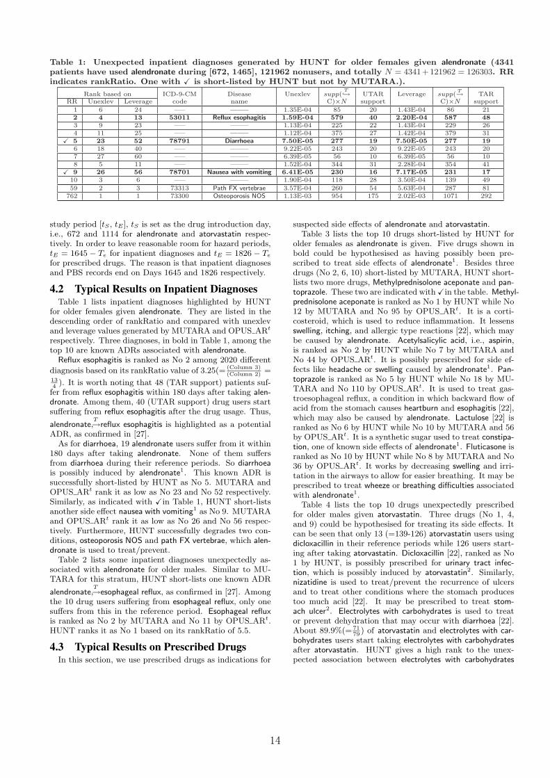
Table 1: Unexpected inpatient diagnoses generated by HUNT for older females given alendronate (4341patients have used alendronate during [672, 1465], 121962 nonusers, and totally N = 4341+121962 = 126303. RRindicates rankRatio. One with X is short-listed by HUNT but not by MUTARA.).

Rank based on ICD-9-CM Disease Unexlev supp(T→ UTAR Leverage supp(

T→ TARRR Unexlev Leverage code name C)×N support C)×N support

1 6 24 —– ——– 1.35E-04 85 20 1.43E-04 86 212 4 13 53011 Reflux esophagitis 1.59E-04 579 40 2.20E-04 587 483 9 23 —– ——– 1.13E-04 225 22 1.43E-04 229 264 11 25 —– ——– 1.12E-04 375 27 1.42E-04 379 31

X 5 23 52 78791 Diarrhoea 7.50E-05 277 19 7.50E-05 277 196 18 40 —– ——– 9.22E-05 243 20 9.22E-05 243 207 27 60 —– ——– 6.39E-05 56 10 6.39E-05 56 108 5 11 —– ——– 1.52E-04 344 31 2.28E-04 354 41

X 9 26 56 78701 Nausea with vomiting 6.41E-05 230 16 7.17E-05 231 1710 3 6 —– ——– 1.90E-04 118 28 3.50E-04 139 49

59 2 3 73313 Path FX vertebrae 3.57E-04 260 54 5.63E-04 287 81762 1 1 73300 Osteoporosis NOS 1.13E-03 954 175 2.02E-03 1071 292

study period [tS , tE ], tS is set as the drug introduction day,i.e., 672 and 1114 for alendronate and atorvastatin respec-tively. In order to leave reasonable room for hazard periods,tE = 1645 − Te for inpatient diagnoses and tE = 1826 − Te

for prescribed drugs. The reason is that inpatient diagnosesand PBS records end on Days 1645 and 1826 respectively.

4.2 Typical Results on Inpatient DiagnosesTable 1 lists inpatient diagnoses highlighted by HUNT

for older females given alendronate. They are listed in thedescending order of rankRatio and compared with unexlevand leverage values generated by MUTARA and OPUS ARt

respectively. Three diagnoses, in bold in Table 1, among thetop 10 are known ADRs associated with alendronate.

Reflux esophagitis is ranked as No 2 among 2020 different

diagnosis based on its rankRatio value of 3.25(= (Column 3)(Column 2)

=134

). It is worth noting that 48 (TAR support) patients suf-fer from reflux esophagitis within 180 days after taking alen-dronate. Among them, 40 (UTAR support) drug users startsuffering from reflux esophagitis after the drug usage. Thus,

alendronateT→reflux esophagitis is highlighted as a potential

ADR, as confirmed in [27].As for diarrhoea, 19 alendronate users suffer from it within

180 days after taking alendronate. None of them suffersfrom diarrhoea during their reference periods. So diarrhoeais possibly induced by alendronate1. This known ADR issuccessfully short-listed by HUNT as No 5. MUTARA andOPUS ARt rank it as low as No 23 and No 52 respectively.Similarly, as indicated with Xin Table 1, HUNT short-listsanother side effect nausea with vomiting1 as No 9. MUTARAand OPUS ARt rank it as low as No 26 and No 56 respec-tively. Furthermore, HUNT successfully degrades two con-ditions, osteoporosis NOS and path FX vertebrae, which alen-dronate is used to treat/prevent.

Table 2 lists some inpatient diagnoses unexpectedly as-sociated with alendronate for older males. Similar to MU-TARA for this stratum, HUNT short-lists one known ADR

alendronateT→esophageal reflux, as confirmed in [27]. Among

the 10 drug users suffering from esophageal reflux, only onesuffers from this in the reference period. Esophageal refluxis ranked as No 2 by MUTARA and No 11 by OPUS ARt.HUNT ranks it as No 1 based on its rankRatio of 5.5.

4.3 Typical Results on Prescribed DrugsIn this section, we use prescribed drugs as indications for

suspected side effects of alendronate and atorvastatin.Table 3 lists the top 10 drugs short-listed by HUNT for

older females as alendronate is given. Five drugs shown inbold could be hypothesised as having possibly been pre-scribed to treat side effects of alendronate1. Besides threedrugs (No 2, 6, 10) short-listed by MUTARA, HUNT short-lists two more drugs, Methylprednisolone aceponate and pan-toprazole. These two are indicated with Xin the table. Methyl-prednisolone aceponate is ranked as No 1 by HUNT while No12 by MUTARA and No 95 by OPUS ARt. It is a corti-costeroid, which is used to reduce inflammation. It lessensswelling, itching, and allergic type reactions [22], which maybe caused by alendronate. Acetylsalicylic acid, i.e., aspirin,is ranked as No 2 by HUNT while No 7 by MUTARA andNo 44 by OPUS ARt. It is possibly prescribed for side ef-fects like headache or swelling caused by alendronate1. Pan-toprazole is ranked as No 5 by HUNT while No 18 by MU-TARA and No 110 by OPUS ARt. It is used to treat gas-troesophageal reflux, a condition in which backward flow ofacid from the stomach causes heartburn and esophagitis [22],which may also be caused by alendronate. Lactulose [22] isranked as No 6 by HUNT while No 10 by MUTARA and 56by OPUS ARt. It is a synthetic sugar used to treat constipa-tion, one of known side effects of alendronate1. Fluticasone isranked as No 10 by HUNT while No 8 by MUTARA and No36 by OPUS ARt. It works by decreasing swelling and irri-tation in the airways to allow for easier breathing. It may beprescribed to treat wheeze or breathing difficulties associatedwith alendronate1.

Table 4 lists the top 10 drugs unexpectedly prescribedfor older males given atorvastatin. Three drugs (No 1, 4,and 9) could be hypothesised for treating its side effects. Itcan be seen that only 13 (=139-126) atorvastatin users usingdicloxacillin in their reference periods while 126 users start-ing after taking atorvastatin. Dicloxacillin [22], ranked as No1 by HUNT, is possibly prescribed for urinary tract infec-tion, which is possibly induced by atorvastatin2. Similarly,nizatidine is used to treat/prevent the recurrence of ulcersand to treat other conditions where the stomach producestoo much acid [22]. It may be prescribed to treat stom-ach ulcer2. Electrolytes with carbohydrates is used to treator prevent dehydration that may occur with diarrhoea [22].About 89.9%(= 71

79) of atorvastatin and electrolytes with car-

bohydrates users start taking electrolytes with carbohydratesafter atorvastatin. HUNT gives a high rank to the unex-pected association between electrolytes with carbohydrates

14

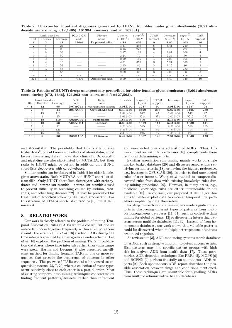
Table 2: Unexpected inpatient diagnoses generated by HUNT for older males given alendronate (1027 alen-dronate users during [672,1465], 101304 nonusers, and N=102331).

Rank based on ICD-9-CM Disease Unexlev supp(T→ UTAR Leverage supp(

T→ TARRR Unexlev Leverage code name (×10−5) C)×N support (×10−5) C)×N support

1 2 11 53081 Esophageal reflux 4.85 402 9 5.82 403 102 5 25 —– ——– 3.41 250 6 3.41 250 63 6 28 —– ——– 3.15 277 6 3.15 277 64 9 33 —– ——– 2.87 106 4 2.87 106 45 15 50 —– ——– 2.24 70 3 2.24 70 36 14 46 —– ——– 2.29 165 4 2.29 165 47 4 13 —– ——– 4.31 358 8 5.27 359 98 16 52 —– ——– 2.15 80 3 2.15 80 39 17 53 —– ——– 2.12 282 5 2.12 282 510 18 55 —– ——– 2.09 86 3 2.09 86 3· · · · · · · · · · · · · · · · · · · · · · · · · · · · · · · · ·323 11 5 73300 Osteoporosis NOS 2.59 134 4 8.40 140 10

Table 3: Results of HUNT: drugs unexpectedly prescribed for older females given alendronate (5,601 alendronateusers during [672, 1646], 121,962 non-users, and N=127,563).

Rank based on ATC Drug Unexlev supp(T→ UTAR Leverage supp(

T→ TARRR Unexlev Leverage code name C)×N support C)×N support

X 1 12 95 D07AC14 Methylprednisolone aceponate 3.08E-04 1247 94 3.08E-04 1247 942 7 44 B01AC06 Acetylsalicylic acid 6.49E-04 3420 233 6.87E-04 3425 2383 19 119 —– ——– 1.82E-04 542 47 1.82E-04 542 474 4 25 —– ——– 1.01E-03 5514 371 1.02E-03 5515 372

X 5 18 110 A02BC02 Pantoprazole 1.86E-04 599 50 2.16E-04 603 546 10 56 A06AD11 Lactulose 3.39E-04 1612 114 5.41E-04 1639 1417 6 32 —– ——– 8.22E-04 595 131 8.51E-04 599 1358 24 121 —– ——– 1.36E-04 788 52 1.81E-04 794 589 15 75 —– ——– 2.39E-04 945 72 4.34E-04 971 98

10 8 36 R03BA05 Fluticasone 5.44E-04 1607 140 7.91E-04 1640 173

and atorvastatin. The possibility that this is attributableto diarrhoea2, one of known side effects of atorvastatin, couldbe very interesting if it can be verified clinically. Dicloxacillinand nizatidine are also short-listed by MUTARA, but theirranks by HUNT might be better. In addition, only HUNTshort-lists electrolytes with carbohydrates.

Similar results can be observed in Table 5 for older femalesgiven atorvastatin. Both MUTARA and HUNT short-list di-cloxacillin. Only HUNT short-lists electrolytes with carbohy-drates and ipratropium bromide. Ipratropium bromideis usedto prevent difficulty in breathing caused by asthma, bron-chitis, and other lung diseases [22]. It may be prescribed fortreatment of bronchitis following the use of atorvastatin. Forthis stratum, MUTARA short-lists nizatidine [10] but HUNTmisses it.

5. RELATED WORKOur work is closely related to the problem of mining Tem-

poral Association Rules (TARs) where a consequent and anantecedent occur together frequently within a temporal con-straint. For example, Li et al [18] studied TARs during thetime intervals specified by a user-given calendar schema. Leeet al [16] explored the problem of mining TARs in publica-tion databases where time intervals rather than timestampswere used. Harms and Deogun [8] also presented an effi-cient method for finding frequent TARs in one or more se-quences that precede the occurrence of patterns in othersequences. The pairwise UTARs can also be viewed as se-quential patterns [25, 7, 20] where a collection of event typesoccur relatively close to each other in a partial order. Mostof existing temporal data mining techniques concentrate onfinding frequent patterns/itemsets, rather than infrequent

and unexpected ones characteristic of ADRs. Thus, thiswork, together with its predecessor [10], complements thesetemporal data mining efforts.

Existing association rule mining mainly works on singlemarket basket database [29] and discovers associations sat-isfying certain criteria [18], or having the highest preference,e.g., leverage in OPUS AR [30]. In order to find unexpectedrules of user interest, Wang et al studied to compare dis-covered rules from data with existing knowledge rules dur-ing mining procedure [29]. However, in many areas, e.g.,medicine, knowledge rules are either innumerable or notavailable [10]. In contrast, our proposed HUNT algorithmaims to better exploit data to discover temporal unexpect-edness implied by data themselves.

Existing research in data mining has made significant ef-forts in discovering different types of patterns from multi-ple homogeneous databases [11, 31], such as collective datamining for global patterns [12] or discovering interesting pat-terns across multiple databases [11, 32]. Instead of from ho-mogenous databases, our work shows that valuable patternscould be discovered when multiple heterogeneous databasesare linked together.

As reviewed in [3], ADR monitoring systems search databases

for ADRs, such as drugT→symptom, to detect adverse events.

Risk patterns may find specific patient groups with highrisk for a given ADR from health data [17]. Those post-market ADR detection techniques like PRRs [5], MGPS [6]and BCPNN [2] perform fruitfully on spontaneous ADR re-ports [9]. Each spontaneous ADR report describes the pos-sible association between drugs and conditions mentioned.Thus, those techniques are unsuitable for signalling ADRsfrom multiple administrative health databases.

15

Table 4: Results of HUNT: drugs unexpectedly prescribed for older males given atorvastatin (6236 atorvastatinusers during [1114, 1646], 78800 non-users, and N=85036).

Rank based on ATC Drug Unexlev supp(T→ UTAR Leverage supp(

T→ TARRR Unexlev Leverage code name C)×N support C)×N support

1 6 98 J01CF01 Dicloxacillin 6.25E-04 993 126 7.67E-04 1006 1392 3 46 —– ——– 1.09E-03 1490 202 1.65E-03 1541 2533 7 103 —– ——– 5.51E-04 466 81 7.25E-04 482 974 4 56 A02BA04 Nizatidine 7.39E-04 1461 170 1.40E-03 1522 2315 9 125 —– ——– 5.01E-04 237 60 5.23E-04 239 626 2 24 —– ——– 2.59E-03 2588 410 2.75E-03 2603 4257 8 90 —– ——– 5.45E-04 1100 127 9.04E-04 1133 1608 11 109 —– ——– 4.82E-04 586 84 6.68E-04 603 101

X 9 13 126 B05BB02 Electrolytes with carbohydrates 4.30E-04 469 71 5.18E-04 477 7910 18 150 —– ——– 3.27E-04 139 38 3.27E-04 139 38

Table 5: Results of HUNT: drugs unexpectedly prescribed for older females given atorvastatin (7,480 atorvastatinusers during [1114, 1646], 90,280 non-users, and N=97,760).

Rank based on ATC Drug Unexlev supp(T→ UTAR Leverage supp(

T→ TAR

RR Unexlev Leverage code name (×10−4) C)×N support C)×N support

1 4 103 —– ——– 4.57 148 56 4.66E-04 149 572 5 99 —– ——– 4.03 530 80 4.98E-04 540 903 7 129 —– ——– 3.18 117 40 3.27E-04 118 414 6 109 —– ——– 3.92 636 87 4.30E-04 640 915 3 52 —– ——– 6.37 1551 181 1.18E-03 1609 2396 10 128 J01CF01 Dicloxacillin 2.63 1036 105 3.29E-04 1043 1127 16 165 —– ——– 1.67 153 28 1.67E-04 153 28

X 8 15 148 B05BB02 Electrolytes with carbohydrates 1.68 452 51 2.25E-04 458 57X 9 13 122 R01AX03 Ipratropium bromide 2.09 321 45 3.60E-04 337 61

10 17 158 —– ——– 1.59 228 33 1.97E-04 232 37

6. CONCLUSIONSBased on our new knowledge representation, Unexpected

Temporal Association Rules (UTARs), we have proposed ainterestingness measure, rankRatio, in the context of sig-nalling unexpected and infrequent patterns characteristic ofADRs from multiple administrative health databases. Wehave developed a simple but effective mining algorithm HUNTto identify pairwise UTARs from the linked health dataset, the QLDS. It has short-listed more known ADRs thanMUTARA. It also has short-listed more interesting UTARswhich may suggest these consequent drugs are possibly pre-scribed for side effects of these antecedent drugs. Consid-ering data biases and incompleteness in the QLDS, theseshortlists would appear to be quite promising, though theystill require careful validation. Thus, the proposed tech-niques can help medical experts generate ADR signals morecomprehensively and effectively.

We have only concentrated on highlighting pairwise UTARsin this paper. However, the proposed mining techniquescan be extended to signal more sophisticated UTARs. Sig-nalling potential ADRs from multiple administrative healthdatabases without any prior specification of drug or condi-tion is also worth further research efforts.

7. ACKNOWLEDGMENTSThe authors acknowledge the Australian Government De-

partment of Health and Ageing (DoHA) and the Queens-land Department of Health for their great support. Theauthors thank R. Sparks and P. Graham from CSIRO, R.Hill, I. Boyd, K. Mackay, J. McEwen, J. Roediger, and C.Winfield from DoHA for their constructive suggestions andcomments.

8. REFERENCES[1] Australian ADR Reporting System.

http://www.tga.gov.au/problem/index.htm.

[2] A. Bate, M. Lindquist, I. Edwards, and R. Orre. Adata mining approach for signal detection andanalysis. Drug Safety, 25(6):393–397, 2002.

[3] D. W. Bates, R. S. Evans, H. Murff, P. D. Stetson,L. Pizziferri, and G. Hripcsak. Detecting adverseevents using information technology. Journal ofAmerican Medical Informatics Association,10(2):115–128, 2003.

[4] C. L. Burgess, C. D. Holman, and A. G. Satti.Adverse drug reactions in older Australians,1981–2002. The Medical Journal of Australia,182(6):267–270, March 2005.

[5] S. Evans, P. Waller, and S. Davis. Use of proportionalreporting ratios for signal generation from spontaneousadverse drug reaction reports. Pharmacoepidemiologyand Drug Safety, 10(6):483–486, Oct-Nov 2001.

[6] D. M. Fram, J. S. Almenoff, and W. DuMouchel.Empirical Bayesian data mining for discoveringpatterns in post-marketing drug safety. In Proceedingsof KDD’03, pages 359–368, 2003.

[7] J. Han, J. Pei, B. Mortazavi-Asl, Q. Chen, U. Dayal,and M.-C. Hsu. FreeSpan: frequent pattern-projectedsequential pattern mining. In Proceedings of KDD’00,pages 355–359, 2000.

[8] S. K. Harms and J. S. Deogun. Sequential associationrule mining with time lags. Journal of IntelligentInformation Systems, 22(1):7–22, 2004.

[9] M. Hauben and X. Zhou. Quantitative methods inpharmacovigilance: focus on signal detection. DrugSafety, 26(3):159–186, 2003.

16

[10] H. Jin, J. Chen, C. Kelman, H. He, D. McAullay, andC. M. O’Keefe. Mining unexpected associations forsignalling potential adverse drug reactions fromadministrative health databases. In PAKDD’06, pages867–876, April 2006.

[11] R. Jin and G. Agrawal. Systematic approach foroptimizing complex mining tasks on multipledatabases. In ICDE’06, page 17, Washington, DC,USA, 2006. IEEE Computer Society.

[12] H. Kargupta, B. Park, D. Hershbereger, andE. Johnson. Collective data mining: A new perspectivetoward distributed data mining. In H. Kargupta andP. Chan, editors, Advances in Distributed DataMining, pages 133–184. AAAI/MIT, 2000.

[13] C. Kelman, S. Perason, R. Day, C. Holman,E. Kliewer, and D. Henry. Evaluating medicines: let’suse all the evidence. Medical Journal of Australia,186(5):249–252, March 2007.

[14] P. E. Langton, G. J. Hankey, and J. W. Eikelboom.Cardiovascular safety of rofecoxib (Vioxx): lessonslearned and unanswered questions. The MedicalJournal of Australia, 181(10):524–525, 2004.

[15] J. Lazarou, B. Pomeranz, and P. Corey. Incidence ofadverse drug reactions in hospitalized patients: ameta-analysis of prospective studies. The Journal ofthe American Medical Association, 279(15):1200–1205,1998.

[16] C.-H. Lee, M.-S. Chen, and C.-R. Lin. Progressivepartition miner: An efficient algorithm for mininggeneral temporal association rules. IEEE Trans.Knowledge Data Eng., 15(4):1004–1017, 2003.

[17] J. Li, A. W.-C. Fu, H. He, J. Chen, H. Jin,D. McAullay, G. Williams, R. Sparks, and C. Kelman.Mining risk patterns in medical data. In Proceedings ofKDD’05, pages 770–775, 2005.

[18] Y. Li, P. Ning, X. S. Wang, and S. Jajodia.Discovering calendar-based temporal association rules.Data & Knowledge Engineering, 44(2):193–218, 2003.

[19] M. Maclure. The case-crossover design: a method forstudying transient effects on the risk of acute events.American Journal of Epidemiology, 133(2):144–153,1991.

[20] H. Mannila, H. Toivonen, and A. I. Verkamo.Discovery of frequent episodes in event sequences.Data Mining and Knowledge Discovery, 1(3):259–289,1997.

[21] D. McAullay, G. Williams, J. Chen, H. Jin, H. He,R. Sparks, and C. Kelman. A delivery framework forhealth data mining and analytics. InV. Estivill-Castro, editor, Twenty-Eighth AustralasianComputer Science Conference (ACSC2005),volume 38, pages 381–390, 2005.

[22] MedlinePlus. http://medlineplus.gov/.

[23] E. Roughead. The nature and extent of drug-relatedhospitalisations in Australia. Journal of Quality inClinical Practice, 19(1):19–22, March 1999.

[24] RxList.http://www.rxlist.com/cgi/generic/atorvastatin ad.htm.

[25] R. Srikant and R. Agrawal. Mining sequentialpatterns: generalizations and performanceimprovements. In Proceedings of EDBT’96, pages3–17, 1996.

[26] M. Stephens, J. Talbot, and P. Routledge, editors.Detection of New Adverse Drug Reactions. MacmillanReference Ltd, London, United Kingdom, 1998.

[27] The Adverse Drug Reactions Advisory Committee. Agut feeling for alendronate. Australian Adverse DrugReaction Bulletin, 18(3), August 1999.

[28] The ICH Expert Working Group. Post-approval safetydata management: Definitions and standards forexpedited reporting. ICH Harmonised TripartiteGuideline, Nov. 2003.http://www.fda.gov/cber/gdlns/ichexrep.htm.

[29] K. Wang, Y. Jiang, and L. V. Lakshmanan. Miningunexpected rules by pushing user dynamics. InProceedings of KDD’03, pages 246–255, 2003.

[30] G. I. Webb. Efficient search for association rules. InProceedings of KDD’00, pages 99–107, 2000.

[31] X. Wu, C. Zhang, and S. Zhang. Databaseclassification for multi-database mining. InformationSystems, 30(1):71–88, 2005.

[32] X. Zhu and X. Wu. Discovering relational patternsacross multiple databases. In ICDE’07, pages 726–735,2007.

17

An Exploration Of Understanding Heterogeneity ThroughData Mining

Haishan LiuUniversity of Oregon

Eugene, Oregon 97403ahoyleo@cs.uoregon.edu

Dejing DouUniversity of Oregon

Eugene, Oregon 97403dou@cs.uoregon.edu

ABSTRACTDevelopment of internet and Web have resulted in many distributedinformation resources which in general are structurally and seman-tically heterogeneous even in the same domain. However, hetero-geneity itself has not been studied in a formal way so that the rep-resentation of different kinds of heterogeneities can be genericallyprocessed by other programs automatically. Most descriptions andcategorization schemes of heterogeneities were given in languagesspecific to different research groups. We believe that efforts in-vested in a thorough research of heterogeneity can ultimately bene-fit both data integration and data mining communities. In this paperwe give a brief survey of various ways to categorize heterogene-ity in the literature, and then performed a case study on detectinga specific class of heterogeneity in the setting of Semantic Webontologies–the one that can be discovered by only data-driven ap-proaches. Finally we propose an automatic ontology matching sys-tem that can detect this heterogeneity by using redescription min-ing techniques. We also believe that automatic ontology matchingprocess is a helpful step in tasks of mining multiple informationsources in the heterogeneous scenario.

Categories and Subject DescriptorsH.2.8 [Database applications]: Data mining—distributed data min-ing; I.2.4 [Knowledge Representation Formalism and Methods]:Ontology; H.3.5 [Information Systems]: Information Storage andRetrieval—data integration

General TermsTheory, Design

KeywordsHeterogeneity, Ontology Matching, Redescription Mining

1. INTRODUCTIONIn both data integration and data mining communities, problems

that might arise due to heterogeneity of multiple data resources are

Permission to make digital or hard copies of all or part of this work forpersonal or classroom use is granted without fee provided that copies arenot made or distributed for profit or commercial advantage and that copiesbear this notice and the full citation on the first page. To copy otherwise, torepublish, to post on servers or to redistribute to lists, requires prior specificpermission and/or a fee.MMIS’08 August 24–27, 2008, Las Vegas, Nevada, USA.Copyright 2008 ACM 978-1-60558-273-3 ...$5.00.

already well known. It is generally agreed to categorize conflictsbetween data resources into structural heterogeneity and semanticheterogeneity [14]. Structural heterogeneity means that differentinformation sources store their data in different structures (e.g., re-lational vs. spreadsheet). Semantic heterogeneity considers differ-ences of the content of data items and their intended meanings. Inmost of the distributed data mining (DDM) literatures, the hetero-geneous scenario is restricted to the case where presumably differ-ent sets of attributes are defined across distributed databases [23]as disjoint models; in other words, data in each local site representthe incomplete knowledge about the complete data set. It is alsotermed as vertical data fragmentation [4].

There are significant progresses made by distributed data miningand information integration researchers in dealing with data hetero-geneity problems. However, many challenges remain. First, Dif-ferent research communities have different terms of definition andtheir focuses vary as well. Different languages specific to particularresearch groups are adopted to describe heterogeneity, which im-pedes effective knowledge sharing and reuse. In this paper we pro-pose to use mapping rules in formal language to categorize hetero-geneity and describe their characteristics. Second, heterogeneity ishard to discover automatically. Most of the current solution of dis-tributed data mining and data integration systems require a step ofmanual specification of correspondences (matchings) in meta-databefore heterogeneity resolution can be carried out. We propose anapproach in this paper to discover meta-data matchings in a highlyautomatic way. We also observe that some kind of heterogeneitycan be detected only by data-driven approaches. In the followingof this paper, the attention is focused on the study of heterogeneityin the setting of Semantic Web ontologies.

In general, an ontology can be defined as the formal specifi-cation of a vocabulary of concepts and the relationships amongthem in a specific domain. In traditional knowledge engineeringand in emerging Semantic Web research, ontologies play an impor-tant role in defining the semantics of data. We explore one kindof heterogeneity in ontologies that can be detected by data-drivenapproaches. A motivating example is given below.

Consider the scenario depicted in figure 1. The left (right) graphshows the structure of the source (target) ontology. The solid tri-angle connected to a node denotes the content of that node. Thedashed dotted line depicts the matching.

As shown in the figure, Vertebrate can be paired to mammal,fish, reptile, amphibian and bird respectively. Any matching algo-rithm that explores the hypernym/hyponym relationship betweenthe labels can discover these correspondences. However, the moreaccurate semantics should be Vertebrate!mammal, fish, reptile,amphibian, bird. The bi-directional arrow in the above expres-sion denotes equivalency, meaning the set of Vertebrate contains

18

M a m m a l

F i s h

R e p t i l e

A m p h i b i a n

B i r d

V e r t e b r a t e

U n i o n

Figure 1: A Motivating Example

no more than the union of mammal, fish, reptile, amphibian andbird. This cannot be verified unless the data of source and target isexamined. We developed novel methods to fulfil this task by meansof matching discovery based on redescription mining techniques.

Redescription mining is a recently proposed approach for datamining tasks in domains which exhibit an underlying richness anddiversity of data descriptors [26, 29, 22]. A redescription is a shift-of-vocabulary, or a different way of communicating informationabout a given subset of data. The goal of redescription mining isto determine the subsets that afford multiple definitions (i.e., de-scriptions) and to find these definitions, which is uniform with theobjective of ontology matching in terms of relating concepts fromdifferent ontologies defined in the same or similar domains.

Ontology matching research is a discipline that aims at facilitat-ing interoperability among different systems in Semantic Web anddatabases. Some ontology-based information integration systemshave been developed to process ontology/schema matching. A sur-vey can be found in [28]. Hence the general idea of our proposedapproach is to recast the problem of ontology matching to discover-ing redescriptions among the named entities, including classes andproperties, in different ontologies.

In terms of redescription, the matching depicted in figure 1 canbe written as:

V ertebrate ! Fish ∪Amphibian ∪Reptile∪Bird ∪Mammal

This is a complex matching since it involves multiple conceptswith a many-to-many correspondence. In some literature it is alsoreferred to as mapping since it specifies the relationship amongthose concepts in terms of a set theory expression, which can beeasily translated to ontology mappings in terms of other formal lan-guages such as First-Order Logic rules. In our previous research,we defined the term “ontology mappings" as formal specificationsof relationships of concepts from different ontologies. Ideally, theyshould be executable by software agents to perform tasks such asdata integration/translation and can be used in distributed data min-ing tasks. We treated the term “ontology matching" as correspon-dence between concepts, which is less formal than mapping rules.Matching discovery is the first step to generate the mapping in ourprevious work. In this paper, we call the proposed data-driven ap-proach. a complex matching discovery process.

During our previous work in data mining and data integration,

we have collected a corpus of real data from different domains 1.A great number of different kinds of heterogeneities have been ob-served.

Below is an example of how a category of heterogeneity, i.e., thenaming conflicts of concepts, can be captured generally using theformal ontology mapping rule (in first-order logic form):∀xP (x) → Q(x);This rule states that class P in the source ontology is mapped

to class Q in the target ontology, where classes in ontology areinterpreted as unary predicates. For example, P and Q can be in-stantiated as person and people, which falls into the synonym sub-category under the naming conflict heterogeneity.

The following rule represents the conflict of property values indifferent ontologies by a mathematical transformation of their val-ues:∀x, yR(x, y) → R′(x, f(y));Here the binary predicates R and R′ denote two properties; x

is the class, and y is the value of the property. For example wecan instantiate this rule with R and R′ being age and birth_year–both are properties of the person class, and the function f meansage = current_year − birth_year.

The rest of the paper is organized as follows. We first introducesome related work in Section 2 and summarize our preliminary un-derstanding of heterogeneities based on our and other groups’ pre-vious work. Then we introduce our framework based on machinelearning and data mining to discover and formally represent theheterogeneities between ontologies (in terms of complex match-ing). We text our methods in two case studies reported in Section 4.We conclude the paper by summarizing our contributions and dis-cussing the future work in Section 5.

2. RELATED WORKS AND BACKGROUND

2.1 Heterogeneity CategorizationVarious ways have been proposed to define different levels of

heterogeneities in the literature. Goh et al[11] identified three maincauses for semantic heterogeneity:

• Confounding conflicts occur when information items seemto have the same meaning, but differ in reality, e.g. due todifferent temporal contexts.

• Scaling conflicts occur when different reference systems areused to measure a value. Examples are different currencies.

• Naming conflicts occur when naming schemes of informa-tion differ significantly. A frequent phenomenon is the pres-ence of homonyms and synonyms.

Noy et al[20] briefly outlined a list of semantic heterogeneity in-cluding using the same linguistic terms to describe different con-cepts; using different terms to describe the same concept; usingdifferent modeling paradigms (e.g., using interval logic or pointsfor temporal representation); using different modeling conventionsand levels of granularity; having ontologies with differing coverageof the domain, and so on.

Won Kim et al developed a framework[15] for enumerating andclassifying the types of multidatabase system (MDBS) structuraland representational discrepancies. The conflicts in a multidatabasesystem were mainly categorized in two cases: schema conflicts anddata conflicts. They concluded that there are two basic causes ofschema conflicts. First is the use of different structures for the same1http://aimlab.cs.uoregon.edu/benchmark

19

information. Second is the use of different specifications for thesame structures. The data conflicts are mainly due to 1) wrongdata violating integrity constraints implicitly or explicitly, and 2)different representations for the same data.

In [12], Hammer et al proposed a systematic classification of dif-ferent types of syntactic and semantic heterogeneities, which wasthen used to compose queries that make up a benchmark systemfor information integration systems. The classification consists oftwelve cases including, for example, synonyms, simple mapping,union types, and etc.

A comprehensive scheme is proposed in [24]. Pluempitiwiriyawejet al classified heterogeneities of XML schemas defined in DTDfiles into three broad classes:

• Structural conflicts arise when the schema of the sources rep-resenting related or overlapping data exhibit discrepancies.Structural conflicts can be detected when comparing the un-derlying DTDs. The class of structural conflicts includesgeneralization conflicts, aggregation conflicts, internal pathdiscrepancy, missing items, element ordering, constraint andtype mismatch, and naming conflicts between the elementtypes and attribute names.

• Domain conflicts arise when the semantic of the data sourcesthat will be integrated exhibit discrepancies. Domain con-flicts can be detected by looking at the information containedin the DTDs and using knowledge about the underlying datadomains. The class of domain conflicts includes schematicdiscrepancy, scale or unit, precision, and data representationconflicts.

• Data conflicts refer to discrepancies among similar or relateddata values across multiple sources. Data conflicts can onlybe detected by comparing the underlying DOCs. The classof data conflicts includes ID-value, missing data, incorrectspelling, and naming conflicts between the element contentsand the attribute values.

2.2 Ontology and Ontology MatchingOntologies, which can be defined as the formal specification of a

vocabulary of concepts and the relationships among them, are play-ing a key role to define data semantics on the Semantic Web [2]and various scientific domains, such as biological and medical datarepositories. The general goal of Semantic Web is to make Webdata machine-“understandable", so that web agents can process andshare information automatically. Many publicly available, struc-turally and semantically rich resources such as databases, XMLdata and the Semantic Web data (e.g., RDF data) provide a uniqueand challenging opportunity to integrate information in new andmeaningful ways. Research involving the Semantic Web is expe-riencing huge gains in standardization in that Web Ontology Lan-guage (OWL [1]) becomes the W3C standard for ontological def-initions in web documents. OWL ontologies mainly consists ofclasses, datatypes and object properties and limited forms of ax-ioms, such as subsumption, inverse relation, cardinality constraintsof classes or properties. OWL also can be used to describe individ-ual objects or data instances.

However, it is extremely unreasonable to expect that ontologiesused for similar domains will be few in number [3]. For example, asthe amount of data collected in the fields of Biology and Medicinegrows at an amazing rate, it has become increasingly important tomodel and integrate the data with ontologies that are scientificallymeaningful and that facilitate its computational analysis. Hence,efforts such as the Gene Ontology (GO [10]) in Biology and the

Unified Medical Language System (UMLS [16]) in Medicine havebeen developed and have become fundamental to researchers work-ing in those domains. However, different labs or organizations maystill use different ontologies to describe their data.

Discovering semantic matchings has been one of major tasksand studied by both Semantic Web and database communities. Re-search in the Semantic Web has resulted in tools for ontology match-ing that are absolutely critical in semantic integration (see [20] fora survey). When two ontologies or two schemas do not have or donot share any data instances, the most straightforward approach isto study the similarity of names and structures of ontological con-cepts or schema attributes. For example, Chimaera [18] providesa ontology editor to allow user to merge ontologies. It suggestspotential matchings based on the names of classes and properties.Protégé [21] gives initial ontology alignments by plugging in oneof existing similarity matching algorithms. BMO [13] can generateblock matchings using a hierarchical bipartition algorithm. Thissystem builds a virtual document for each ontology and compareseach pair of concepts with the information in the virtual document.

If two ontologies share data instances, the most straightforwardway to compare them is to test the intersection of their instancesets. GLUE [6] is a system that employs multiple machine learn-ing techniques to semi-automatically discover one-to-one match-ings between two ontology taxonomies. The idea of the approachis to calculate the joint distributions of the classes, instead of com-mitting to a particular definition of similarity. Thus, any particularsimilarity measure can be computed as a function over the jointdistributions. iMAP [5] is a system that semi-automatically dis-covers one-to-one and even complex matchings between relationaldatabase schemas. The idea is to reformulated the matching prob-lem as a search in a match space.

2.3 Redescription MiningRedescription mining was first studied in [26]. Ramakrishnan et

al. defined a redescription as a shift-of-vocabulary, or a differentway of communicating information about a given subset of data in-stances. They also introduced CARTwheels algorithm to exploit theduality between class partitions and path partitions in an inducedclassification tree to model and mine redescriptions. Later in [29],Zaki and Ramakrishnan proposed an alternative algorithm to mineall minimal (non-redundant) redescriptions underlying a dataset us-ing notions of minimal generators of closed itemset. Parida andRamakrishnan [22] formally studied the space of redescriptionsunderlying a dataset and characterize their intrinsic structure. Italso analyzed when mining redescriptions is feasible and how tocustom-build a mining system for various biases.

In order to perform redescription mining algorithm to match on-tologies, a universal set of instances of the ontologies should bespecified in advance. This falls under the problem of object recon-ciliation. Object reconciliation problem is studied for determiningwhether two different data instances refer to the same real-worldentity. It is closely related to instance-based matching approaches.The research in [7] proposed methods to address the reconciliationproblem within the same schema. The algorithm takes three steps.It first construct the dependency graph based on the taxonomy in-formation. Every node in the graph consists of one pair of entitieswhich denotes a potential reconciliation decision. Second, it iter-atively computes the similarity scores of reconciliation decisions.The similarity score of one reconciliation decision can both affectand be affected by the similarity score of its neighbors. The algo-rithm terminated when a fixed point is reached. Finally, transitiveclosure is computed to determine the final reconciliation decisions.

Our work is an extension of redescription mining in ontology

20

matching to study heterogeneity. We focus on the scenario thattwo ontologies both have data instances and some of them referto the same real-world entities. We extend the CARTwheels algo-rithm to incorporate ontology structure heuristics to guide its searchin the space of redescriptions and to find more complex ontologymatchings rather than one-to-one matchings. We also explore a newmethod to reconcile the instances described by different ontologiesso that to generate a universal dataset for our redescription miningbased ontology matching algorithm.

3. SYSTEM FRAMEWORKHere we present our ontology-based approach using redescrip-

tion mining to detect the specific class of heterogeneity discussed insectoin 1. We assume that ontologies of given datasets are obtainedin advance by either human specification or automatic extractionby machine from (semi-)structured data sources. There are severalapproaches proposed to investigate the transformation of relationalschemas to ontologies (see [27, 17, 19]).

The proposed approach generally consists of following steps:first, parse the OWL document to extract both its the ontologystructural information and data instances; second, perform the ob-ject reconciliation algorithm to construct a universal dataset; thenperform the extended redescription mining process to discover com-plex ontology matchings.

We have also developed an ontology parser reported in [8], whichcan translate the OWL ontologies to our internal representation(Web-PDDL) of our ontology-based integration system. It facili-tates the access and manipulation of the taxonomy information ofthe ontologies, and also extracts the instances from the input on-tologies and prepares them as the input to the object reconciliationprocessor. Below we describe in detail about our object reconcilia-tion and extended redescription mining algorithms.

3.1 Object ReconciliationIn order to perform the redescription mining algorithm to match

ontologies, it is necessary to determine a universal set of data ob-jects. To fulfil this objective, we must be able to compare ontologyinstances with each other and decide if they represent the same realworld objects. Note that it is not guaranteed for the instances indifferent ontologies to be overlapping. For example, personnel on-tologies used by different institutions may have totally different in-stances. Redescription mining is not directly suitable for matchingtasks in such situations. Hence the existence of a set of equiva-lent instances will serve as the basic assumption in the proposedapproach.

One possible approach to establish equivalence between two ob-jects is to make use of a so-called correspondence function [9]:given two objects as input, the correspondence function determinesthe degree of equivalence between the two. However, it is very hardto design such a correspondence function since matchings betweenthe ontologies that describe the data objects are yet unknown, thuscompromising the comparison of objects in the elaborate level ofgranularity. We propose to address this problem by using machinelearning techniques that implicitly incorporate ontology structureinformation and achieve satisfactory result with even very simplecorrespondence function.

Consider finding the overlapping instances in ontology O1 andO2 in Figure 2, specifically, the overlapping instances of the setst1, t2, t3, t4, t5, t6 and s1, s2, s3, s4, s5, s6. Instead of apply-ing the correspondence function directly to all instances in differ-ent ontologies as shown in Figure 3, we propose a way to partioninstances into sub-groups and apply the correspondence functionto the instances in the related sub-groups. We first train a learner

X 1

X 2 X 3

X 4 X 5

Y 1

Y 2 Y 3

Y 5 Y 6

Y 4

t5 , t6

t1 , t2 t3 , t4 s 1 , s 2 s 3 , s 4

s 5 , s 6

O 1 O 2

Figure 2: Two taxonomies of different ontologies.

t 1t 2t 3t 4t5t6

s 1s 2s 3s 4s 5s 6

Figure 3: Applying the correspondence function directly to theinstances of two ontologies.

based on the instances of O1 with the target label being the classesin O1, namely, X1, X2, X3, X4 and X5; then we apply the learnedmodel to predict the class labels of the instances in O2. This pro-cess partitions the instances in O2 according to O1. Finally, the cor-respondence function is applied between all the pairs of instancesin the groups that have the same class label, as shown in Figure 4,supposing s3 and s4 are predicted to belong to class X4 in O1 (thepredicted class is denoted by X ′

4 in the figure), and so forth.In our implementation of the first test case described in detail in

the experiment section, we used a simple string similarity measureas the correspondence function. Specifically, we treated the contentof the instances in a bag-of-word representation. The classificationprocess is essentially a text categorization process.

t 1t 2

s 3s 4

X 4 X 4 ’

t 3t 4

s 1s 2

X 5 X 5 ’

t 5t 6

s 5s 6

X 3 X 3 ’

Figure 4: Applying the correspondence function to the relatedsubsets of instances.

21

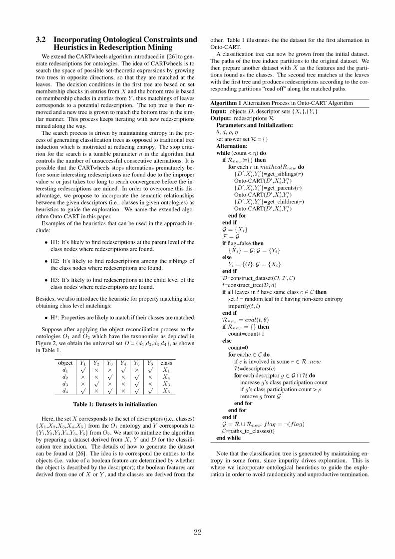
3.2 Incorporating Ontological Constraints andHeuristics in Redescription Mining

We extend the CARTwheels algorithm introduced in [26] to gen-erate redescriptions for ontologies. The idea of CARTwheels is tosearch the space of possible set-theoretic expressions by growingtwo trees in opposite directions, so that they are matched at theleaves. The decision conditions in the first tree are based on setmembership checks in entries from X and the bottom tree is basedon membership checks in entries from Y , thus matchings of leavescorresponds to a potential redescription. The top tree is then re-moved and a new tree is grown to match the bottom tree in the sim-ilar manner. This process keeps iterating with new redescriptionsmined along the way.

The search process is driven by maintaining entropy in the pro-cess of generating classification trees as opposed to traditional treeinduction which is motivated at reducing entropy. The stop crite-rion for the search is a tunable parameter n in the algorithm thatcontrols the number of unsuccessful consecutive alternations. It ispossible that the CARTwheels stops alternations prematurely be-fore some interesting redescriptions are found due to the impropervalue n or just takes too long to reach convergence before the in-teresting redescriptions are mined. In order to overcome this dis-advantage, we propose to incorporate the semantic relationshipsbetween the given descriptors (i.e., classes in given ontologies) asheuristics to guide the exploration. We name the extended algo-rithm Onto-CART in this paper.

Examples of the heuristics that can be used in the approach in-clude:

• H1: It’s likely to find redescriptions at the parent level of theclass nodes where redescriptions are found.

• H2: It’s likely to find redescriptions among the siblings ofthe class nodes where redescriptions are found.

• H3: It’s likely to find redescriptions at the child level of theclass nodes where redescriptions are found.

Besides, we also introduce the heuristic for property matching afterobtaining class level matchings:

• H*: Properties are likely to match if their classes are matched.

Suppose after applying the object reconciliation process to theontologies O1 and O2 which have the taxonomies as depicted inFigure 2, we obtain the universal set D = d1,d2,d3,d4, as shownin Table 1.

object Y1 Y2 Y3 Y4 Y5 Y6 classd1

√ × × √ × √X1

d2 × × √ × √ × X4

d3 × √ × × √ × X3

d4√ × √ × √ √

X5

Table 1: Datasets in initialization

Here, the set X corresponds to the set of descriptors (i.e., classes)X1,X2,X3,X4,X5 from the O1 ontology and Y corresponds toY1,Y2,Y3,Y4,Y5, Y6 from O2. We start to initialize the algorithmby preparing a dataset derived from X , Y and D for the classifi-cation tree induction. The details of how to generate the datasetcan be found at [26]. The idea is to correspond the entries to theobjects (i.e. value of a boolean feature are determined by whetherthe object is described by the descriptor); the boolean features arederived from one of X or Y , and the classes are derived from the

other. Table 1 illustrates the the dataset for the first alternation inOnto-CART.

A classification tree can now be grown from the initial dataset.The paths of the tree induce partitions to the original dataset. Wethen prepare another dataset with X as the features and the parti-tions found as the classes. The second tree matches at the leaveswith the first tree and produces redescriptions according to the cor-responding partitions “read off" along the matched paths.

Algorithm 1 Alternation Process in Onto-CART AlgorithmInput: objects D, descriptor sets Xi,YiOutput: redescriptions R

Parameters and Initialization:θ, d, ρ, ηset answer set R = Alternation:while (count < η) do

if Rnew!= thenfor each r in mathcalRnew do

D′,X ′i ,Y ′

i =get_siblings(r)Onto-CART(D′,X ′

i ,Y ′i )

D′,X ′i ,Y ′

i =get_parents(r)Onto-CART(D′,X ′

i ,Y ′i )

D′,X ′i ,Y ′

i =get_children(r)Onto-CART(D′,X ′

i ,Y ′i )

end forend ifG = XiF = Gif flag=false thenXi = G;G = Yi

elseYi = G;G = Xi

end ifD=construct_dataset(O,F , C)t=construct_tree(D, d)if all leaves in t have same class c ∈ C then

set l = random leaf in t having non-zero entropyimpurify(t, l)

end ifRnew = eval(t, θ)if Rnew = then

count=count+1else

count=0for eachc ∈ C do

if c is involved in some r ∈ R_newH=descriptors(c)for each descriptor g ∈ G ∩H do

increase g’s class participation countif g’s class participation count > ρremove g from G

end forend for

end ifG = R∪Rnew; flag = ¬(flag)C=paths_to_classes(t)

end while

Note that the classification tree is generated by maintaining en-tropy in some form, since impurity drives exploration. This iswhere we incorporate ontological heuristics to guide the explo-ration in order to avoid randomicity and unproductive termination.

22

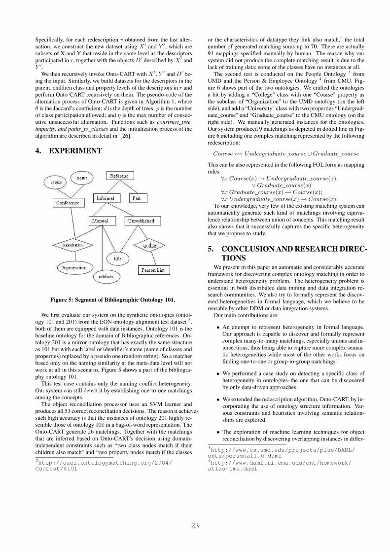
Specifically, for each redescription r obtained from the last alter-nation, we construct the new dataset using X ′ and Y ′, which aresubsets of X and Y that reside in the same level as the descriptorsparticipated in r, together with the objects D′ described by X ′ andY ′.

We then recursively invoke Onto-CART with X ′, Y ′ and D′ be-ing the input. Similarly, we build datasets for the descriptors in theparent, children class and property levels of the descriptors in r andperform Onto-CART recursively on them. The pseudo-code of thealternation process of Onto-CART is given in Algorithm 1, whereθ is the Jaccard’s coefficient; d is the depth of trees; ρ is the numberof class participation allowed; and η is the max number of consec-utive unsuccessful alternation. Functions such as construct_tree,impurify, and paths_to_classes and the initialization process of thealgorithm are described in detail in [26].

4. EXPERIMENT

Figure 5: Segment of Bibliographic Ontology 101.

We first evaluate our system on the synthetic ontologies (ontol-ogy 101 and 201) from the EON ontology alignment test dataset 2.both of them are equipped with data instances. Ontology 101 is thebaseline ontology for the domain of Bibliographic references. On-tology 201 is a mirror ontology that has exactly the same structureas 101 but with each label or identifier’s name (name of classes andproperties) replaced by a pseudo one (random string). So a matcherbased only on the naming similarity at the meta-data level will notwork at all in this scenario. Figure 5 shows a part of the bibliogra-phy ontology 101.

This test case contains only the naming conflict heterogeneity.Our system can still detect it by establishing one-to-one matchingsamong the concepts.

The object reconciliation processor uses an SVM learner andproduces all 53 correct reconciliation decisions. The reason it achievessuch high accuracy is that the instances of ontology 201 highly re-semble those of ontology 101 in a bag-of-word representation. TheOnto-CART generate 26 matchings. Together with the matchingsthat are inferred based on Onto-CART’s decision using domain-independent constraints such as “two class nodes match if theirchildren also match" and “two property nodes match if the classes2http://oaei.ontologymatching.org/2004/Contest/#101

or the characteristics of datatype they link also match," the totalnumber of generated matching sums up to 70. There are actually91 mappings specified manually by human. The reason why oursystem did not produce the complete matching result is due to thelack of training data; some of the classes have no instances at all.

The second test is conducted on the People Ontology 3 fromUMD and the Person & Employee Ontology 4 from CMU. Fig-ure 6 shows part of the two ontologies. We crafted the ontologiesa bit by adding a “College" class with one “Course" property asthe subclass of “Organization" to the UMD ontology (on the leftside), and add a “University" class with two properties “Undergrad-uate_course" and “Graduate_course" to the CMU ontology (on theright side). We manually generated instances for the ontologies.Our system produced 9 matchings as depicted in dotted line in Fig-ure 6 including one complex matching represented by the followingredescription:

Course ! Undergraduate_course ∪Graduate_course

This can be also represented in the following FOL form as mappingrules:

∀x Course(x) → Undergraduate_course(x);∨Graduate_course(x)

∀x Graduate_course(x) → Course(x);∀x Undergraduate_course(x) → Course(x).

To our knowledge, very few of the existing matching system canautomatically generate such kind of matchings involving equiva-lence relationship between union of concepts. This matching resultalso shows that it successfully captures the specific heterogeneitythat we propose to study.

5. CONCLUSION AND RESEARCH DIREC-TIONS

We present in this paper an automatic and considerably accurateframework for discovering complex ontology matching in order tounderstand heterogeneity problem. The heterogeneity problem isessential in both distributed data mining and data integration re-search communities. We also try to formally represent the discov-ered heterogeneities in formal language, which we believe to bereusable by other DDM or data integration systems.

Our main contributions are:

• An attempt to represent heterogeneity in formal language.Our approach is capable to discover and formally representcomplex many-to-many matchings, especially unions and in-tersections, thus being able to capture more complex seman-tic heterogeneities while most of the other works focus onfinding one-to-one or group-to-group matchings.

• We performed a case study on detecting a specific class ofheterogeneity in ontologies–the one that can be discoveredby only data-driven approaches.

• We extended the redescription algorithm, Onto-CART, by in-corporating the use of ontology structure information. Var-ious constraints and heuristics involving semantic relation-ships are explored.

• The exploration of machine learning techniques for objectreconciliation by discovering overlapping instances in differ-

3http://www.cs.umd.edu/projects/plus/DAML/onts/personal1.0.daml4http://www.daml.ri.cmu.edu/ont/homework/atlas-cmu.daml

23

P e r s o n E m p o l y e e

A d d r e s s O r g a n i z a t i o n

e m a i l A d d r e s s

a g e

s e x

t i t le

b i r t h d a y

h o m e p h o n e

w o r k p h o n e

n a m e

a l u m n u s w o r k F o r

a d d r e s s _ s t a t e

a d d r e s s _ z i p a d d r e s s _ s t r e e t

a d d r e s s _ c i t y

w o r k A d d r e s s

P e r s o n E m p l o y e e

s e x

n a m e _ p e r s o n

a g e

job- t i t le

e x p e r t i s e

h a s - e m p l o y e s

e m p l o y e r

o f f i ce

s t a r t - d a t e

e n d - d a t e

e m a i l

M i s s i o n

n a m e _ o r g a n i z a t i o n

a d d r e s s

p h o n e

b u i l d i n g

l a b

O r g a n i z a t i o n O f f i c e

p h o t o

I m a g e

s u b c l a s s s u b c l a s s

C o l l e g e

s u b c l a s s

U n i v e r s i t y

s u b c l a s s

U n d e r g r a d u a t e _ c o u r s e G r a d u a t e _ c o u r s eC o u r s e

Figure 6: UMD and CMU person ontologies.

ent ontologies, and thus enabling the construction of a uni-versal reconciled dataset for further mining algorithms.

In the future work, we plan to extensively explore the spectrumof heterogeneities with more real-world data from different do-mains stored in relational databases, XML documents or spread-sheets. We will further study the formal methodology to representand categorize data heterogeneities and continue to develop algo-rithms to automatically resolve heterogeneity. We also plan to dis-cover ontology matchings by combining the conceptual level andinstance level approach in an effective and efficient manner. In ourfuture work, there are mainly several challenges that need to beaddressed:

• One big difficulty for the ontology matching system that adoptsinstance level approach is the orthogonality of data. If thereare no overlapping instances supplied by the ontologies un-der consideration, it will be very hard to perform mining al-gorithms. What are the more intrinsic characteristics of dataand how to study them effectively deserve further study.

• Not all data heterogeneities can be represented in formal lan-guage as mappings or the expressions with set theories. Onthe other hand, even with sophisticated design, it is hard toget 100% accurate mappings without human involvement.Each mapping may have some associated probabilistic val-ues. Similar to what we have reported in [25], the mappingrules discovered by inductive logic programming have accu-racy for each rule.

• Although we argue that formal mappings rules can be used

by DDM or data integration systems because the rules aremachine processable, it is an open question whether existingDDM or data integration systems can process all discovereddata heterogeneities. We may need to design different DDMor data integration algorithms for different kinds of hetero-geneities.

• Besides the existing repositories that contain heterogeneousdata, it is hard to find appropriate datasets for the purpose oftesting and benchmarking the performance of systems thatdesigned to detect and resolve heterogeneity. Most of therepositories do not have golden standards for heterogeneityresolution.

On the other hand, the existing data repository (e.g., our col-lected data5) has only limited resources so that only a subsetof heterogeneities is exhibited in the data. For some specificstudy in DDM or data integration, researchers may requiredifferent kinds of combinations of heterogeneities, which isnot easily satisfied by any existing datasets. A benchmarksystem with the capability to automatic generate syntheticdata according to user’s demand of certain heterogeneitieswill be very helpful.

6. ACKNOWLEDGEMENTSWe thank the anonymous reviewers for their insightful comments

and helpful suggestion for the improvements of our work.

5http://aimlab.cs.uoregon.edu/benchmark

24

7. REFERENCES[1] OWL Web Ontology Language.

http://www.w3.org/TR/owl-ref/.[2] T. Berners-Lee, J. Hendler, and O. Lassila. The Semantic

Web. Scientific American, 284(5), May 2001.[3] J. D. Bruijn and A. Polleres. Towards an Ontology Mapping

Specification Language for the Semantic Web. Technicalreport, Digital Enterprise Research Institute, June 2004.

[4] D. Caragea, J. Z. 0002, J. Bao, J. Pathak, and V. Honavar.Algorithms and software for collaborative discovery fromautonomous, semantically heterogeneous, distributedinformation sources. In ALT, pages 13–44, 2005.

[5] R. Dhamankar, Y. Lee, A. Doan, A. Y. Halevy, andP. Domingos. iMAP: Discovering Complex Mappingsbetween Database Schemas. In Proceedings of the ACMConference on Management of Data, pages 383–394, 2004.

[6] A. Doan, J. Madhavan, P. Domingos, and A. Y. Halevy.Learning to Map Between Ontologies on the Semantic Web.In International World Wide Web Conferences (WWW),pages 662–673, 2002.

[7] X. Dong, A. Halevy, and J. Madhavan. Referencereconciliation in complex information spaces. In SIGMOD,pages 85–96, 2005.

[8] D. Dou, D. V. McDermott, and P. Qi. Ontology Translationon the Semantic Web. Journal of Data Semantics, 2:35–57,2005.

[9] D. Fang, J. Hammer, and D. McLeod. The identification andresolution of semantic heterogeneity in multidatabasesystems, 1994.

[10] T. Gene Ontology Consortium. Creating the Gene OntologyResource: Design and Implementation. Genome Research,11(8):1425–1433, 2001.

[11] C. H. Goh. Representing and reasoning about semanticconflicts in heterogeneous information systems. PhD thesis,1997. Supervisor-Stuart E. Madnick.

[12] J. Hammer, M. Stonebraker, and O. Topsakal. Thalia: Testharness for the assessment of legacy information integrationapproaches. In ICDE, pages 485–486, 2005.

[13] W. Hu and Y. Qu. Block matching for ontologies. In Proc. of5th International Semantic Web Conference, Athens, GA,USA, November 5-9, 2006, LNCS 4273, 2006.

[14] W. Kim and J. Seo. Classifying schematic and dataheterogeneity in multidatabase systems. Computer,24(12):12–18, 1991.

[15] W. Kim and J. Seo. Classifying schematic and dataheterogeneity in multidatabase systems. Computer,24(12):12–18, 1991.

[16] D. Lindberg, B. Humphries, and A. McCray. The UnifiedMedical Language System. Methods of Information inMedicine, 32(4):281–291, 1993.

[17] L. Lubyte and S. Tessaris. Extracting ontologies fromrelational databases. In Description Logics, 2007.

[18] D. L. McGuinness, R. Fikes, J. Rice, and S. Wilder. TheChimaera Ontology Environment. In Proceedings of theNational Conference on Artificial Intelligence, pages1123–1124, 2000.

[19] B. Motik, I. Horrocks, and U. Sattler. Bridging the gapbetween owl and relational databases. In WWW, pages807–816, 2007.

[20] N. F. Noy. Semantic integration: A survey of ontology-basedapproaches. SIGMOD Record, 33(4):65–70, 2004.

[21] N. F. Noy and M. A. Musen. PROMPT: Algorithm and Toolfor Automated Ontology Merging and Alignment. InProceedings of the National Conference on ArtificialIntelligence, pages 450–455, 2000.

[22] L. Parida and N. Ramakrishnan. Redescription mining:Structure theory and algorithms. In AAAI, pages 837–844,2005.

[23] B. Park and H. Kargupta. Distributed data mining:Algorithms, systems, and applications, 2002.

[24] C. Pluempitiwiriyawej and J. Hammer. A ClassificationScheme for Semantic and Schematic Heterogeneities in XMLData Sources. University of Florida, Gainesville, FL,technical report tr000-004 edition, September 2000.

[25] H. Qin, D. Dou, and P. LePendu. Discovering ExecutableSemantic Mappings Between Ontologies. In Proceedings ofthe International Conference on Ontologies, Databases andApplication of Semantics (ODBASE), pages 832–849, 2007.

[26] N. Ramakrishnan, D. Kumar, B. Mishra, M. Potts, and R. F.Helm. Turning cartwheels: an alternating algorithm formining redescriptions. In KDD, pages 266–275, 2004.

[27] L. Stojanovic, N. Stojanovic, and R. Volz. Migratingdata-intensive web sites into the semantic web. In SAC ’02:Proceedings of the 2002 ACM symposium on Appliedcomputing, pages 1100–1107, New York, NY, USA, 2002.ACM Press.

[28] H. Wache, T. Vogele, U. Visser, H. Stuckenschmidt,G. Schuster, H. Neumann, and S. Hubner. Ontology-basedintegration of information: A survey of existing approaches.In IJCAI–01 Workshop: Ontologies and InformationSharing, pages 108–117, 2001.

[29] M. J. Zaki and N. Ramakrishnan. Reasoning about sets usingredescription mining. In KDD, pages 364–373, 2005.

25

Multiclass Multifeature Split Decision Tree Construction ina Distributed Environment

Jie OuyangIntelligent Information

Engineering LabDepartment of ComputerScience and Engineering

Oakland University, Rochester,MI 48309

jouyang@oakland.edu

Nilesh PatelIntelligent Information

Engineering LabDepartment of ComputerScience and Engineering

Oakland University, Rochester,MI 48309

npatel@oakland.edu

Ishwar SethiIntelligent Information

Engineering LabDepartment of ComputerScience and Engineering

Oakland University, Rochester,MI 48309

isethi@oakland.edu

ABSTRACTThe decision tree-based classification is a popular approach for pat-tern recognition and data mining. Most decision tree inductionmethods assume training data being present at one central loca-tion. Given the growth in distributed databases at geographicallydispersed locations, the methods for decision tree induction in dis-tributed settings are gaining importance. This paper describes onesuch method that generates compact trees using multifeature splitsin place of single feature split decision trees generated bymost ex-isting methods for distributed data. Our method is based on Fisher’slinear discriminant function, and is capable of dealing with multi-ple classes in the data. For homogeneously distributed data, thedecision trees produced by our method are identical to decisiontrees generated using the Fisher’s linear discriminant function withcentrally stored data. For heterogeneously distributed data, a cer-tain approximation is involved with a small change in performancewith respect to the tree generated with centrally stored data. Exper-imental results for several well known data sets are presented andcompared with decision trees generated using the Fisher’s lineardiscriminant function with centrally stored data.

Categories and Subject DescriptorsI.5 [Computing Methodologies]: PATTERN RECOGNITION

General TermsAlgorithms, Performance

1. INTRODUCTIONThe decision tree-based classification is a popular approach for

pattern recognition and data mining. Methods for the induction ofdecision trees have been studied for past several decades. Oncebuilt, a decision tree can be used to classify previously unseen in-stances of patterns or to characterize patterns of different classes inthe form of rules to constitute a knowledge base for decisionsup-

Permission to make digital or hard copies of all or part of this work forpersonal or classroom use is granted without fee provided that copies arenot made or distributed for profit or commercial advantage and that copiesbear this notice and the full citation on the first page. To copy otherwise, torepublish, to post on servers or to redistribute to lists, requires prior specificpermission and/or a fee.MMIS ’08, August 24, 2008, Las Vegas, Nevada, USA.Copyright 2008 ACM 978-1-60558-273-3 ...$5.00.

port. The decision tree methodology has been applied to numerousapplications in different domains. A comprehensive survey of de-cision tree induction methods from multiple disciplines and theirapplications is provided by Murthy[12]. Almost all methodsre-viewed in this survey are based on the assumption that the trainingdata for building the decision tree is present at one centralsite.

With increasing globalization of businesses, advances in technol-ogy, and increasing concerns about the loss of privacy due todatamining, the interest in data mining methods that can operatein adistributed data environment has been growing. While it is alwayspossible to move data to one central location for mining, thecostsfor such a move can be high. Consequently, methods for decisiontree induction in a distributed data environment without large scalemovement of data have started receiving attention. A distributeddata environment can be homogeneous or heterogeneous. In a ho-mogeneous environment, different sites record similar informationalbeit for different objects. The distributed data in such situationsis also termed as horizontally partitioned data. In a heterogeneousenvironment, all sites record information for the same set of objectsalbeit different aspects of the information. Such data is referred asvertically partitioned data. Of course in reality, data maybe bothhorizontally and vertically partitioned.

Two basic approaches to distributed decision tree induction arepossible. One approach is to have an ensemble of decision treeswith each data site contributing its own local decision treeto theensemble. Examples of some popular ensemble methods are boost-ing, bagging, and random forests. Any of these methods can beemployed in a distributed environment. One problem with ensem-ble approach is the difficulty of converting the ensemble decisionto rules to form a knowledge base. Another drawback is that itapplies only to the horizontally partitioned data scenario. A novelwork in this type of approach is the orthogonal decision trees dueto Kargupta et al [10] where the Fourier transformation of trees isused to combine them to arrive at a final decision tree. The otherapproach to distributed decision tree induction is to develop onlyone single decision tree by organizing the computation for atra-ditional decision tree induction method at one site in such awaythat traffic between different data sites is minimized. The result-ing decision tree then can be used by each site independentlyif sodesired. This approach is applicable to both the horizontally andthe vertically partitioned data scenarios. Furthermore, the resultingsingle decision tree is useful for a knowledge base across the entireenterprise. Examples of this approach are exemplified by theworksdescribed in [5][2]. In both cases, single feature decisiontrees arebuilt for discrete features using entropy or Gini index as splittingcriteria. Since building single feature decision trees with discrete

26

features needs only different counts to evaluate different features aspotential split candidates, the extension to the distributed data en-vironment is achieved easily. These methods are, however, difficultto extend even to single feature decision trees when data consistsof continuous features. In such situations, choosing a split requiressearching through potential cutoff values across different features.Thus, there does not appear any efficient method of computationwith distributed data that can deal with continuous features.

In this paper, we suggest a method for decision tree induction ina distributed environment. Our method is based on Fisher’s lineardiscriminant function [7] to generate multifeature splitsfor deci-sion tree nodes. Since Fisher’s discriminant function is meant fortwo class problems, we suggest a method to extend it to multiclassproblems. For homogeneously distributed data, the decision treesproduced by our method are identical to decision trees generatedusing the Fisher’s linear discriminant function with centrally storeddata. For heterogeneously distributed data, a certain approximationis involved with a small change in performance with respect to thetree generated with centrally stored data. The organization of thepaper is as follows. Section 2 reviews some related work. Section 3discusses distributed fisher’s linear discriminant and shows differ-ent relationships in the partitioned data that are used for buildingthe decision tree in a distributed environment. Section 4 discussesextension to multiple classes by clustering classes into two superclasses. Section 5 presents the final algorithm followed by experi-mental results in Section 6. Finally a summary of the work is pro-vided in Section 7.

2. RELATED WORKThe most common approach for building a decision tree clas-

sifier in a distributed setting uses the tree aggregation techniquewhich combines the locally trained classifiers into a singledecisiontree. Researchers have suggested numerous tree ensebling tech-niques. Lazarevic et al[11] suggested a distributed boosting algo-rithm for homogeneously distributed data which combines the lo-cal classifiers into a weighted voting ensemble on each disjoint dataset. Prodromidis et al[14] proposed a distributed meta-learning en-vironment, in which the local classifiers are transfered to acen-tral site. The predictions of local classifiers on the central data isused to form the training set for meta learner. Finally an arbiter orcombiner is used to determine the final classification results. In adifferent work, Park et al[13] proposed a decision tree method forheterogeneously partitioned data. He combined the boosting andtree ensemble techniques where a measure was defined to selectmisclassified instances to train decision trees. Finally a Fouriertransformation based method is used to ensemble decision treesfrom local data sites. Caragea et al[4][5] proposed a different ap-proach for distributed learning. He decomposed the learning tasksinto two components; (1) hypothesis generation and (2) informa-tion extraction. The information extraction part is extended to dis-tributed environment while the hypothesis generation partis keptcentral. The information extracted by the information extractorsis fed to the hypothesis generator. As long as the information ex-tracted is the same in distributed and centralized settings, the hy-pothesis generator produces the same hypothesis. Hence their dis-tributed algorithms are apodictic to their centralized counterpart,which is termed exact distributed learning. Caragea suggested thedistributed information extraction based on sufficient statistics. Hefurther demonstrated applicability of his approach on decision treeinduction for both horizontally and vertically partitioned data. Aslight extension of Caragea’s work is also found in [4], where headdressed the issue of counting examples from heterogeneous andautonomous data sources by the query system INDUS[6]. These

approaches generate single feature decision trees which are moreappropriate for categorical features rather then numerical features.

Giannella et al[8] proposed a method for decision tree induc-tion for a heterogeneous environment. His method uses the featuresplitting criteria which tries to reduce the coordination cost for de-termining instances of current tree node. Instead of keeping a copyof node assignment at the local site, the algorithm tries to determinethe tree node instances when it is to be split. The procedure is basedon the dot product of binary vectors which are node assignment in-dicators of different sites. To reduce the communication cost of thebinary vectors, a random projection method is used to reducetheirdimensionality. The information loss caused by the random projec-tion is also analyzed. Baik et al[1] suggested a different method forreducing the intra node communication. He proposed encoding ofnode assignment bit vectors. Both these approaches also generatesa single feature split decision trees.

Bar-Or et al[2] suggested a distributed decision tree algorithmfor data sites organized in a hierarchical structure. Such structuremoves the information through a path from the leaf data site to theroot data site. In principle, this algorithm is more suitable for hor-izontally partitioned data. The method defines the lower andupperbound of the gain function which is further used to efficiently col-lect gain values using the hierarchical structure. Their approach issuitable for any high dimension data, provided that the correlationsin it are sparse.

3. DISTRIBUTED DECISION TREE INDUC-TION USING FISHER’S LINEAR DISCRIM-INANT

Decision Tree is among the most important non-parametric tech-nique for building classifiers. Decision tree algorithms such asC4.5[15] or CART[3] have attracted many researchers because itsability to provide intuitive interpretations. The standard decisiontree build process follows a top-down divide and conquer tech-nique, in which the induction starts with a root node containing alldata. The tree nodes are then recursively partitioned untila stop-ping condition is satisfied. Early decision tree induction methodsfollowed a single feature split technique. In this technique, onefeature with the greatest gain function value is picked for split-ting the tree. Single feature split decision trees could grow verylarge leading to suboptimal accuracy. Multifeature decision treeinduction techniques are introduced to overcome the size and per-formance issues. The later technique splits the data using combi-nation of features. If the combination criterion is linear,the treeis called linear discriminant tree. One method to determinethefeature combination coefficients is using perceptron learning[16].Another method is to use Fisher’s Linear Discriminant(FLD)[7] assuggested in [17].

3.1 Fisher’s Linear Discriminant(FLD)Fisher’s Linear Discriminant aims at finding the projectionvec-

tor W(combination coefficient vector) such that the projection ofthe original data has the best discriminant ability. Given aset ofaugmented training vectors,X1,X2, ...,Xn, from two classesC1

andC2, FLD tries to determineW such that it maximizes -

W = maxW

WT (m1 −m2)(m1 −m2)TWWT (S1 + S2)W

, (1)

wheremi andSi are the mean and the scatter matrix of classi re-spectively. The solution of Eq.1 can be represented as -

W = (S1 + S2)−1(m1 −m2). (2)

27

Assuming the projection of each class to be one dimensional Gaus-sian, the splitting threshold can be easily computed using the jointpoint,W0, of two Gaussian Probability Distribution Functions(PDFs).One well known issue with FLD is possible singularity of (S1+S2),making it difficult to obtained its inverse. This difficulty is oftentriggered by mismatch between number of data point instances withrespect to its dimensionality. Principle Component Analysis(PCA)is used as one common practice to overcome this problem. Specifi-cally, PCA is used to reduce the dimensionality of input databeforeFLD is applied. It should be noted that FLD is more suitable fornumerical data, although the non-numeric data can also be trainedto generate a decision tree using suitable preprocessing (data trans-formation) technique.

3.2 Statistics Required by FLDThe decision tree algorithm proposed in this paper is based on

performing FLD in a distributed environment. As established in thesubsection3.1, this requires computation of class means and scat-ters and thereby computing the projection vector that separates thetwo classes of data. In this section we establish the theoretical foun-dation to compute the class means and scatters in a homogeneousand heterogeneous distributed environment. Without loss general-ity, we consider the case of two data sites. Lets further considerone of these two sites to be a coordinating or a master site whichalso contains one partition of the data. Hence the datasetDn×d, isdivided among two sites, consider these to beX andY. Lets definefew terms which are central to our algorithm.

• Global Mean(m):Represents the mean of the total dataset.

• Global Scatter(S ):Represents the scatter (covariance) of thetotal dataset.

• Global Class Mean(mi ): Represents the mean of the data be-longing to classi.

• Global Class Scatter(Si): Represents the scatter (covariance)of the data belonging to classi.

• Local Class Mean(mi, j ): Represents the mean of the data be-longing to classi available at sitej.

• Local Class Scatter(Si, j ): Represents the scatter (covariance)of the data belonging to classi available at sitej.

Table.1 summarize the denotations of these different statistics. In

Statistics Global Global LocalStatistics Class Statistics Class Statistics

mean m mi mi, j

scatter S Si Si, j

Table 1: Statistics Required by FLD in Distributed Settings

the following subsection we introduce the theoretical foundation tocompute these statistics in a homogeneously and heterogeneouslypartitioned data.

3.2.1 Computing FLD Statistics in Homogeneous Set-ting

Consider dataDn×d being homogeneously partitioned betweentwo sites. LetX andY be the data partitions ofd dimensions where

n = nX + nY, Dn×d =

[

XY

]

. Given this distribution we can easily

compute class mean(mi ) and global mean(m) as -

mi, j =

∑

i, jXi, j

ni, j(3)

mi =

∑

jmi, jni, j

∑

jni, j

(4)

m=

∑

imini

∑

ini

(5)

Eq.4 and Eq.5 are computed at the master site. The communicationcost for transferringmi, j andni, j in the distributed environment ofK sites isO(KCd) whereC is the number of classes. AssumingDbeing zero mean, which can be achieved by shifting all the data byits global mean, the scatter ofD can be calculated as -

SD =

[

XY

]T [XY

]

(6)

=[

XT X + YTY]

= SX + SY

Generalizing Eq6 toK sites leads us to the solution -

Si =∑

j

Si, j (7)

S =k∑

i=0

Si (8)

The communication cost for transferringSi, j in an environment ofK sites isO(KCd2). Assumingd << n, K << n, andC << n, thetotal communication costKCd2

<< nd.

3.2.2 Computing FLD Statistics in a HeterogeneousSetting

It is conceivable that distributed data is not always partitionedhomogeneously (data split by samples). Many situations necessi-tates data split by its dimensionality. Such distribution is also refer-eed as vertical or heterogeneous data partitioning. LetX andY bethe data partitions with the conditiond = dX + dY. The data matrixD is denoted byD =

[

X Y]

. Again, without loss of generality wecan compute the means as -

mi =[

mi,1mi,2...mi,K]

(9)

m=

∑

imini

∑

ini

(10)

Again assumingD be the zero mean dataset, we can computescatter as -

SD =[

X Y]T [

X Y]

(11)

=

[

XT X XTYYTX YTY

]

=

[

SX XTYYTX SY

]

.

To calculate the nonlocal(off diagonal) items in Eq.11, one of thedata partitions needs to be transferred to the master site, which isundesirable. HenceSD has to be approximated. We can accomplishthis in two ways which are both based on approximating original

28

data using truncated singular value decomposition(SVD)[9]. As-sume dataX needs to be transferred to whereY is located. We canfactorizeX to its singular values as -

X = UΣV = U1Σ1,1VT1 + ... + UdXΣdX ,dX VT

dX, (12)

where the matrixV(right eigen vector matrix) contains a set of or-thonormal input or the basis vector directions forX, the matrixU(left eigen vector matrix) contains a set of orthonormal outputbasis vector directions forX, and the matrixΣ contains the singularvalues. The singular values are also considered scalar gaincon-trols. The first item in the expansion, the basis vector directions forX, contains the most information ofX, we can useU1Σ1,1VT

1 onlyto approximateX, denoted byX = U1Σ1,1VT

1 .Our first method approximatingSD aims computing as many ex-

act entries( entries with the same values inSD and its approxima-tion) as possible. Hence the sub-matricesXTY andYTX are respec-tively approximated byXTY andYT X while SX is an exact entrycomputed byV ∗ΣT ∗Σ ∗V. This approximation requires transmis-sion of onlyU1, Σ, andV, keeping the communication cost down toO(n+ d2) for two sites environment. Thus for an environment ofKsites, the cost is scaled toO(Kn+Kd2), orO(Kn) whend << n. Theapproximation ofXTY andYTX loses some information. The loseof information may lead to drop in overall classifier performance,which can be addressed by transferring more than 1, sayp, vectorsfrom U. The cost of communication then would beO(Kpn). Thesecond method is based on approximating the entire dataset.In thismethod, every local site performs SVD on locally stored dataandsends its ownU1, Σ, andV to the master site. The master site thenforms an approximation of the original dataset, and computes thescatter in a centralized manner. The difference of this method isthat only local items are exact entries inSD, e.g, SX will be re-placed with its approximation. Ironically, both techniques have thesame communication cost model.

The information transfer in method 1 can be done in a serial orparallel manner. In the serial approach, every site needs storagespace for the information from the previous site only. However inmethod 2, the master site needs storage space to hold informationfrom all local sites. On the contrary, method 2 requires one timeinformation transfer during the whole tree induction process whilemethod 1 requires information transfer for every tree node split.The implementation implication is the trade-off between space andtransmission.

4. MULTICLASS CLASSIFICATION USINGHIERARCHICAL SUPER CLASSING

The Fisher’s Linear Discriminant algorithm was originallypro-posed for a two class problem. Over these years, researchershaveproposed numerous FLD extensions to solve the multiclass prob-lems. For example, the authors of [17] have suggested the useof exchange method for reducing multiclass problems to two-classproblems. However the exchange method does not fit well for adistributed environment. To cope with multiclass problems, wepropose use of hierarchical structuring of the data and apply tradi-tional class method on this pre-organized data. Our solution keepsthe problem formation simple in a distributed environment.Thehierarchical structuring orders the data to transform the multiclassproblem to a two class problem. We generate this hierarchy byes-timating two super classes. This is accomplished by hierarchicallyclustering the class means at the master site. The super class assign-ment is then sent to each local sites to get the statistics of the superclasses. The super class means and scatters are obtained using theprocess outlined in previous section using Eq.3 and Eq.7. One is-

D a t a

L S

. . . . .

M S

C o m p u t e m i , j . . k , S i , j . . k , s p l i t l o c a l t r e e n o d e

m i , j . . k

C o m p u t e m s c 1 , s c 2 ,S s c 1 , s c 2 ,p e r f o r m P C A , F L D

n i , j . . k

S i , j . . k

m

WW 0

D a t a D a t a D a t a

1 L S 2 L S 3 L S K

Figure 1: Induction of Distributed Multifeature Decision Tree

sue of the super class generation is what class mean to use. Theclass mean can be computed in the original space, in the full scaleprinciple component space, or in the reduced principle componentspace. We performed the experiment using each to evaluate thedifference in classifier performance. Our empirical study did notobserve significant performance difference between each method.The experiment results reported in this paper uses the classmeansin the full scale principle component space.

In short, Principal Component Analysis, Hierarchical Super Class-ing, and Fisher’s Linear Discriminant constitute three keycompo-nents of our algorithm. These three steps are carried out iterativelyin the following manner -

1 Compute PCA to gets a full scale eigen vector matrix.

2 Calculate Global class means in the eigen vector space.

3 Generate Super classes using the class means from step [2].

4 Compute Super class means and scatters(Ssc1,Ssc2).

5 Asses the singularity ofSsc1 + Ssc2.

6 Remove the least significant eigen vector and repeat step 4and 5, if assessed close to singular; otherwise performanceFLD to compute projection vectorW.

It shall be noted that the repetition of step 4 does not require extracommunication. It is performed by removing certain vectorsfromthe means and scatters.

5. INDUCTION OF DISTRIBUTED MULTI-FEATURE DECISION TREE(DMDT)

The generalized Distributed Multifeature Decision Tree solutionis depicted in Figure 1. Consider the data, containingL classes, be-ing distributed amongK sites denoted asLS1, LS2, ..., LSk. Let usdenote the central or master site to beMS. Although our algorithmspecifically suggest separate master site, it is equally applicable ina peer to peer setting where there is no functional coordinator. Insuch situation, any one of the local site can fulfill this rolemastersite. Clearly, each participating site is responsible for computing itslocal class means (mi, j ) and local class scatter (Si, j). Furthermore,the local sites are also responsible for maintaining the decision tree.The master site is responsible for performing PCA, dividingthe

29

data among super classes, and computing the projection plane us-ing the FLD. Following pseudo code captures the steps involved ininduction of a multifeature decision tree in a distributed environ-ment. For completeness, we outline three pseudo code algorithms,one for homogeneous and two for heterogeneous data distributions.The use of→ signifies the data transmission direction.

Algorithm 1 DMDT in Homogeneous Environment1: ∀ j ∈ K and∀i ∈ L, Compute(mi, j ,ni, j )→ MS2: LS j ← Compute(m)3: Compute(Si, j )→ MS4: Compute(S) @ MS5: PCA@ MS6: LS j ← GenerateSuperclass(S C1,S C2)7: LS j ← Compute(msc1 ,msc2)8: Compute(Ssc1, j ,Ssc2, j )→ MS9: Compute(Ssc1 ,Ssc1) @ MS

10: while Singular(Ssc1 + Ssc2) do11: Remove the least significant principle component.12: end while13: FLD @ MS14: LS j ← (W, W0)

Please note that the transmission ofm to LS j can be saved in im-plementation as the global data can be made zero mean by makingeach local dataset zero mean. The two algorithms for the hetero-geneous environment correspond to the two approximation solu-tions described in section 3.2. The first pseudo code describes thecomputation steps carried out at each non-leaf tree node, while thesecond piece of pseudo code describes the tree induction process.

Algorithm 2 DMDT in Heterogeneous Environment 11: ∀ j ∈ K and∀i ∈ L, Compute(mi, j ,ni, j )→ MS2: ∀ j ∈ K, S VD(U1...p, j ,Σ j ,Vj)→ MS3: Compute(mi , S) @ MS4: PCA@ MS5: GenerateSuperclass(S C1, S C2) @ MS6: Compute(msc1, msc2, Ssc1, Ssc2) @ MS7: while Singular(Ssc1 + Ssc2) do8: Remove the least significant principle component.9: end while

10: FLD @ MS11: LS j ← (W, W0)

Algorithm 3 DMDT in Heterogeneous Environment 21: ∀ j ∈ K, S VD(U1...p, j ,Σ j ,Vj)→ MS2: ∀ j ∈ K, Compute(U1...p, j ∗ Σ j ∗ Vj) @ MS3: Compute(FLDT) @ MS

Once the tree induction process is complete, we perform the clas-sification to assess the performance of our classifier. Classificationof the new instance for homogeneous distributed environment is nodifferent than the centralized setting. Since each site carriesa copyof the decision tree, new data is classified immediately without anycommunication overhead. It is not the same for the heterogeneousdistribution of data. It requires the data transformation before clas-sification. Considerx be the feature partition of a new instance atsite j. Let Σ j andVj be the components obtained by SVD of thetraining samples atj. The row inU for x can be obtained from

x× Vj × (Σ j )−1. The transformation ofx is computed as -

x = (x× Vj × (Σ j )−1)1...p × Σ j × Vj (13)

x is then sent to the master site to fill in its position in the approx-imated instances. The approximated instance is then classified atthe master site.

6. ACCURACY EXPERIMENTAL RESULTSTo assess the performance of our decision tree constructed in a

distributed environment, we compared its accuracy againsta cen-trally build decision tree. The experiments are conducted over 13UCI datasets. The data sizes range from couple hundreds to severalthousands and the dimensions range from 5 to 65. To test the abil-ity of DMDT to process multiclass problems, the class numbers ofthese datasets range from 2 to 10. In addition, the complexity of thedatasets varies as the accuracy of some popular decision tree algo-rithms on them ranges from around 50% to around 90%. In orderto check the accuracy of our classifier, we performed two runsoffive folds cross validation on each dataset.

The first experiment measures the accuracy of distributed classi-fier in both homogeneous and heterogeneous environments with re-spect to the centralized version. To simulate a homogeneousdistri-bution of 4 sites, we first permuted the data instances and then par-titioned it in 4 random segments. Each segment is then distributedto four virtual processing sites. Due to relatively small dimension-ality, we simulate the heterogeneous distribution using only 3 sites.In this setting, the features are evenly partitioned and distributedamong available 3 sites. In addition, each site receives a copy ofthe class labels. It shall be noted that heterogeneous distributionis only tested on the datasets having greater than six features. Theconstraint was necessary to ensure that each site receives at leasttwo features. The experimental results are tabulated in Table.2.Column with titleHetero 1shows the results from algorithm2 whilethe column titledHetero 2corresponds to algorithm3. Both are ob-tained with the number of left eigen vectors, denoted byp = 1.

Dataset Classes Instances Features Centralized Homo Hetero 1 Hetero 2

Breast 2 683 10 96.63±1.26 96.93±1.78 96.93±0.76 96.78±0.62

Bupa 2 345 7 67.83±2.25 68.99±4.79 62.90±3.15 64.35±4.49

Vote 2 435 17 95.63±0.90 95.86±1.81 93.10±3.07 94.71±1.81

Ionosphere 2 351 35 88.03±3.40 89.18±1.97 89.18±3.09 90.02±2.55

Wine 3 178 14 98.31±1.44 98.32±1.45 88.18±4.49 88.19±2.27

Iris 3 150 5 97.33±2.62 97.33±2.62 - -

Car 4 1728 7 85.39±2.02 88.34±1.68 76.1±3.10 79.28±0.73

Dermatology 6 358 35 97.48±1.10 97.48±2.35 63.41±8.65 84.09±5.43

Segment 7 2310 20 91.16±6.2 92.66±6.32 78.40±5.86 84.29±5.33

Zoo 7 108 18 92.10±7.86 91.1±3.92 83.10±5.51 90.05±3.41

Glass 7 214 10 57.89±8.47 57.48±4.21 64.03±3.53 61.69±4.94

Optdigits 10 3823 65 94.45±0.49 95.19±0.97 34.5±8.37 80.49±0.99

Pendigits 10 7494 17 95.26±0.40 97.67±0.72 86.18±11.37 80.33±10.10

Table 2: Performance of Distributed Multifeature DecisionTree

As expected, the performance of DMDTs in a homogeneous en-vironment is same as Linear Discriminant Tree in a centralized en-vironment. However, in heterogeneous environment, performancedrops are observed for both algorithms for most datasets. Insomecases, the observed drops are significant. This is due to use ofonly first left eigen vector in our approximation process. Itis also

30

observed that the performance drops do not have any strong cor-relation with the average number of features per site. Algorithm3has systematically outperformed algorithm2. The reason for that isobserved in the consistency of approximated scatter matrix, whichwas found to be better in algorithm3 than algorithm2.

The second experiment measures the impact ofp on the perfor-mance. In this case, the results are obtained only using algorithm3as Table2 shows algorithm3 outperforms algorithm2. The columntitled Featuresrepresents the average number of features at eachsite. The value ofp is increased by one for each trial. The exper-iment was stopped as soon as the accuracy obtained with certainp value is close to the accuracy of the centralized version. Table3

Dataset Classes Features Centralized p=1 p=2 p=3 p=6

Breast 2 3.33 96.63±1.26 96.78±0.62 - - -

Bupa 2 2.33 67.83±2.25 64.35±4.49 68.12±1.37 - -

Vote 2 5.67 95.63±0.90 94.71±1.81 95.63±1.61 - -

Ionosphere 2 11.67 88.03±3.40 90.02±2.55 - - -

Wine 3 4.67 98.31±1.44 88.19±2.27 97.76±2.2 - -

Car 4 2.33 85.39±2.02 79.28±0.73 87.85±2.24 - -

Dermatology 6 11.67 97.48±1.10 84.09±5.43 92.72±2.58 93.57±1.51 96.92±1.74

Segment 7 6.67 91.16±6.2 84.29±5.33 92.55±0.99 - -

Zoo 7 6 92.10±7.86 90.05±3.41 99.05±2.01 - -

Glass 7 3.33 57.89±8.47 61.69±4.94 62.58±4.76 - -

Optdigits 10 21.67 94.45±0.49 80.49±0.99 88.1±1.27 90.17±2.89 93.28±2.4

Pendigits 10 5.67 95.26±0.40 80.33±10.10 90.73±3.67 95.72±1.19 -

Table 3: Impact of p on Heterogeneous Data Distribution

captures the results of our second experiment run measuringtheimpact ofp. It is apparent that in most cases (9 datasets out of 12)our method reports comparable results with less than half ofthecommunication bandwidth requirement.

Third, we compare the performance of DMDT with two popu-lar decision tree algorithms, ID3 and CART. We only refer to theexperimental results of their centralized versions since the theoret-ical proof described in[4][5] shows that the performance ofexactdistributed learning will be the same as its centralized counterpart.The comparison is shown in Table4. We quote the accuracy ofID3 and CART from [17]. The performance for heterogeneoussettings is only presented for algorithm3 withp set to 1 since itoutperforms algorithm2. The comparison shows that the DMDT

Dataset ID3 CART Homo Hetero 2

Breast 94.1±1.2 94.9±1.4 96.93±1.78 96.78±0.62

Bupa 62.3±5.3 61.7±3.4 68.99±4.79 64.35±4.49

Vote 94.9±1.1 90.3±3.2 95.86±1.81 94.71±1.81

Ionosphere 87.6±3.2 86.8±4.0 89.18±1.97 90.02±2.55

Wine 88.7±3.7 87.3±4.4 98.32±1.45 88.19±2.27

Iris 93.9±2.8 89.3±4.4 97.33±2.62 -

Car 81.0±1.3 83.8±2.0 88.34±1.68 79.28±0.73

Dermatology 92.8±2.4 80.9±4.6 97.48±2.35 84.09±5.43

Segment 91.1±1.2 88.1±1.7 92.66±6.32 84.29±5.33

Zoo 91.3±6.3 69.9±9.7 91.1±3.92 90.05±3.41

Glass 60.7±6.2 53.9±4.2 57.48±4.21 61.69±4.94

Optdigits 78.4±1.5 81.4±2.1 95.19±0.97 80.49±0.99

Pendigits 85.7±1.0 87.1±2.9 97.67±0.72 80.33±10.10

Table 4: Performance Comparison

algorithm systematically performs better than ID3 and CARTinhomogeneous settings. This is because DMDT’s more suitablefor

describing oblique decision surfaces. Also fisher’s lineardiscrimi-nant analysis increases the generality of the decision tree. The per-formance of algorithm3 is comparable to ID3 and CART for mostof the datasets even with the smallest possiblep setting. For thosethree datasets(Dermatology, Segment, and Pendigits) withperfor-mance loss for more than 5 percent, similar or better performanceof DMDT can be reached whenp is set to 2(see Table3), which isa small number compared to the dimensionality.

7. CONCLUSIONIn this paper, we propose a multifeature decision tree algorithm

for distributed environment. Our approach extends the popularFisher’s Linear Discriminant in a straightforward fashionto dealwith homogeneous data distribution. The correctness of thethe-oretical proof showing the equivalency between centralized anddistributed algorithm for homogeneously distributed datais fur-ther verified using the experimental results. For heterogeneouslydistributed data, we introduced the data approximation technique.Two data approximation approaches are suggested and comparedfor their relative performances. Our experimental resultsshow thatthe consistency in estimating scatter matrix considerablyimprovesthe classification performance. Although, the communication costof implementing algorithm for heterogeneous environment is pro-portional to the total number of data instances, we empirically provedthat our approach could reach the performance of a centralized ver-sion while saving more than half of the communication cost. Alsowe empirically demonstrated distributed multifeature decision treescan reach similar or better performance than the distributed singlefeature decision trees with low communication cost in both homo-geneous and heterogeneous environments.

8. REFERENCES[1] S. Baik and J. W. Bala. A decision tree algorithm for

distributed data mining: Towards network intrusiondetection. InICCSA, pages 206–212, 2004.

[2] A. Bar-Or, A. S. R. Wolff, and D. Keren. Decision treeinduction in high dimensional, hierarchically distributeddatabases. InIn Proceedings of 2005 SIAM InternationalConference on Data MiningS DM′05, Newport Beach, CA,April 2005.

[3] L. Breiman, J. Friedman, R. Olshen, and C. Stone.Classification and Regression Trees. Wadsworth and Brooks,Monterey, CA, 1984.

[4] D. Caragea, A. Silvescu, and V. Honavar. Decision treeinduction from distributed heterogeneous autonomous datasources. InProceedings of the 3rd International Conferenceon Intelligent Systems Design and Applications, pages341–350, Tulsa, OK, 2003.

[5] D. Caragea, A. Silvescu, and V. Honavar. A framework forlearning from distributed data using sufficient statistics andits application to learning decision trees.InternationalJournal of Hybrid Intelligent Systems, 2003.

[6] J. A. R. Castillo, A. Silvescu, D. Caragea, J. Pathak, andV. G. Honavar. Information extraction and integration fromheterogeneous, distributed, autonomous information sourcesca federated ontology-driven, query-centric approach. InIEEE International Conference on Information Integrationand Reuse, Las Vegas, Nevada, 2003.

[7] R. O. Duda, P. E. Hart, and D. G. Stork.PatternClassification. Wiley-Interscience, 2000.

[8] C. Giannella, K. Liu, T. Olsen, and H. Kargupta.Communication efficient construction of decision trees over

31

heterogeneously distributed data. InProceedings of theFourth IEEE International Conference on Data Mining,pages 67–74, 2004.

[9] T. W. H. Qi and D. Birdwell.Statistical Data Mining andKnowledge Discovery, chapter Chapter 19: Global PrincipalComponent Analysis for Dimensionality Reduction inDistributed Data Mining. CRC Press, 2004.

[10] H. Kargupta and B.-H. Park. A fourier spectrum-basedapproach to represent decision trees for mining data streamsin mobile environments.IEEE Transactions on Knowledgeand Data Engineering, 16(2):216–229, 2004.

[11] A. Lazarevic and Z. Obradovic. The distributed boostingalgorithm.In Knowledge Discovery and Data Mining, pages311–316, 2001.

[12] S. K. Murthy. Automatic construction of decision treesfromdata: A multi-disciplinary survey.Data Mining andKnowledge Discovery, 2(4):345–389, 1998.

[13] B. Park, R. Ayyagari, , and H. Kargupta. A fourieranalysis-based approach to learn classifier from distributedheterogeneous data. InIn Proceedings of the first SIAMInternational Conference on Data Mining, Chicago, IL,April 2001.

[14] A. Prodromidis and P. Chan.Advances of Distributed DataMining, chapter Meta-learning in Distributed Data MiningSystems: Issues and Approaches. MIT/AAAI Press, 2000.

[15] J. R. Quinlan.C4.5: Programs for Machine Learning.Morgan Kaufmann, 1992.

[16] I. Sethi and J. Yoo. Design of multicategory multifeaturesplit decision trees using perceptron learning.PatternRecognition, 27(7):939–947, 1994.

[17] O. T. Yildiz and E. Alpaydin. Linear discriminant trees. InProc. 17th International Conf. on Machine Learning, pages1175–1182, San Francisco, CA, 2000. Morgan Kaufmann.

32

A Novel Approach for Discovering Chain-Store High Utility Patterns in a Multi-Stores Environment

Guo-Cheng Lan and Vincent S. Tseng* Department of Computer Science and Information Engineering

National Cheng Kung University, Tainan, Taiwan, R.O.C. Email: tsengsm@mail.ncku.edu.tw

ABSTRACT Utility mining is an emerging topic in the field of data mining in recent years. A high utility pattern contains both important factors such as profit and quantity. The patterns can be composed of items with low frequency and high profit, or those with high frequency and low profit. However, the existing methods on utility mining were mostly designed for a centralized database and not suitable for the environment with multiple data sources like a chain-store enterprise. Moreover, the existing methods do not take important factors like on-shelf periods and locations of items into consideration. In this paper, we proposed a new kind of pattern named Chain-Store High Utility Pattern that contains not only individual profit and quantity of items but also common selling periods and stores of items in a multi-stores environment. Moreover, we proposed a new method named CS-Mine (Chain-Store High Utility Pattern Mine) for discovering the proposed patterns efficiently. The CS-Mine algorithm needs only to scan the database twice and it can effectively filter out a large number of unnecessary itemsets with the filtration mechanism. To our best knowledge, this is the first work on mining chain-store high utility patterns in a multi-stores environment. Through a series of experiments, our proposed method was shown to deliver excellent performance under varied system conditions.

Categories and Subject Descriptors H.2.8 [Database Management]: Data Mining

General Terms Algorithms, Performance, Design, Experimentation, Theory.

Keywords Data mining, utility mining, high utility patterns, chain-store patterns, multi-stores environment.

1. INTRODUCTION In the fields of data mining, the association rules model [3] is the most frequently discussed issue due to its wide applications. In [2], Agrawal et al. first proposed the Apriori algorithm that is the most

well-known algorithm for mining association rules from a transaction database. However, since the association rules model assumes that the significance or profit of each product is the same, we cannot understand the represented significance of each product in a product combination. Moreover, the methods on association rules mining may fail to discover product combinations which are composed of items with low frequency and high profit, or those with high frequency and low profit in a transactional database. Hence, frequency is not sufficient to answer a product combination whether it is highly profitable or whether it has a strong impact.

For the above reasons, Chan et al. [5] proposed a new topic named utility mining that discovers high utility patterns from a transactional database. A high utility pattern on utility mining [8][12][17][18] considers both individual profit of each product in a database and bought quantity of each product in a transaction simultaneously. Thus high utility patterns can represent practical utility value of each product in a product combination. However, a product may be put on-shelf and taken off-shelf multiple times or that some products are only sold in some stores in a chain-store enterprise. Thus the base of existing methods in computing utility value of a product set is throughput a database so the results discovered by existing methods may be biased in a multi-stores environment.

In order to solve the above problems, we proposed a new pattern named chain-store high utility pattern, which takes both of the selling periods and the selling stores into consideration in a multi-stores environment. An example pattern is like “In the afternoon, customers usually purchase high-priced gifts and a gift card together in stores near the hospitals”. In such kind of patterns, the itemsets may not be frequent, while it may be a high utility one since most customers do not buy these items. Besides, we also proposed a new mining method named CS-Mine that can efficiently discover the proposed patterns in a multi-stores environment. The concept of CS-Mine algorithm is similar to EFI algorithm [9], but CS-Mine only scans the database two times and reduces the overhead in determining the relationship between items. Then CS-Mine decomposes transactions to generate directly subsets via the filtration mechanism. To our best knowledge, this is the first work on mining chain-store high utility patterns in a multi-stores environment. Through a series of experimental evaluation, we measured the differences between original and proposed patterns and CS-Mine was shown to have good performance under different conditions.

The remaining parts of this paper are organized as follows. The related work is described in Section 2. The problem definition is stated in Section 3. The proposed method CS-Mine is

Permission to make digital or hard copies of all or part of this work for personal or classroom use is granted without fee provided that copies are not made or distributed for profit or commercial advantage and that copies bear this notice and the full citation on the first page. To copy otherwise, or republish, to post on servers or to redistribute to lists, requires prior specific permission and/or a fee. MMIS'08, August 24, 2008, Las Vegas, Nevada, USA Copyright 2008 ACM 978-1-60558-273-3…$5.00.

33

described in Section 4. Experiments to demonstrate the differences between proposed and original patterns by varying various parameters and the performance of the CS-Mine algorithm in dealing with large databases are described in Section 5. Conclusions and future work are given in Section 6.

2. RELATED WORK In the fields of data mining, association rules are widely applied to many applications. However, since the frequency is not sufficient to measure the significance of association rules, Agrawal et al. [14] proposed the quantitative association rules in 1996 and Cai et al. [5] proposed the weighted association rules method in 1998. On the other hand, temporal association rules mining [4][11][13] has been proposed to solve the dynamic association rules problem, but the discovered results may be incorrect because they consider the occurred periods of transactions not the on-shelf periods of products, and the on-shelf and off-shelf periods of products may be switched multiple times in a transactional database. Since previous data mining models are mostly based on a centralized database and traditional association rules are not sufficient to provide knowledge inherent in data across the stores in a chain-store enterprise, the focus of many studies [1][7][16] is how to develop data mining techniques on multiple databases. Among these studies, Chen et al. [7] proposed a novel approach named Apriori_TP which is different from other approaches because the approach discovers temporal association rules across the stores in a multi-stores environment. Besides, the rules [7] consider both selling periods and selling stores of products into consideration simultaneously. In [7], they use the common selling periods and stores of all products in a product combination as relative content of a product set to compute the relative support, and then discover frequent relative itemsets in a multi-stores environment.

Nevertheless, all of the above studies assume that the significances or profits of items are the same in the mining process. In order to overcome the problem, Chan et al. [8] proposed an importance topic named utility mining. The concept behind the utility mining is to discover the high utility itemsets whose utility values satisfy the minimum utility threshold given by users from a transactional database. Utility mining considers simultaneously both individual profit of each product in a database and bought quantity of each product in a transaction in the mining processes. In [18], the authors proposed the definitions of utility mining and theoretical model named MEU. However, the theoretical model MEU has to examine complete sets of all items to find all high utility itemsets. Thus Liu et al. [12] proposed a novel algorithm named Two-Phase to increase the performance in terms of discovering high utility itemsets from a database. However, the existing methods [8][12][15][17][18] on utility mining are not suitable for the environment with multiple data sources.

As described above, there exists no work for discovering high utility itemsets in a multi-databases environment. This motivates our exploration of the issue of efficiently mining high utility itemsets in a multi-databases environment.

3. PROBLEM DEFINITION In order to describe our problem clearly, a set of terms leading to the formal definitions of utility mining and multiple database

mining problems can be formally defined as follows by referring to [7] and [18].

Definition 1. Let T = t1, t2, ..., ti, ... be a set of mutually disjoint time periods, where ti denotes the ith time period in the complete periods, T.

Definition 2. Let P = p1, p2, ..., py, ... be a set of stores, where py denotes the the yth store in a chain-store enterprise.

Definition 3. Let I = i1, i2, ..., im be a set of items. Furthermore, let D = Tran1, Tran2, …, Tranj be a transactional database with multiple data sources, where each transaction Tranj is a subset of I. In D, each transaction Tranj is attached with a timestamp, ti, and store identifier, py, to indicate the occurred store py and the occurred time ti of the transaction.

Definition 4. Let an itemset X in transaction Tranj be a set of items, where X⊆ I and X⊆ Tranj. If |X| = k, the itemset X is represented as a k-itemset. If X⊆ Tranj, the set of transactions containing the itemset X are denoted as W(X, D) = Tranj| Tranj ∈D∧ X⊆ Tranj.

Definition 5. Let the content of an itemset X, VX, be the combination of the common selling periods and stores of all items in an itemset X that all items are sold concurrently. For example, if the itemset X is composed of the items IL and IZ, the content of the itemset X is represented as VX = VL∩ VZ.

Definition 6. o(Im, Tranj), local transaction utility value, represents the quantity of item Im in transaction Tranj.

Definition 7. s(Im), external utility, represents the corresponding utility value of each item in the utility table. Note that the users can set the value of each item to inflect the importance of each item in the utility table.

Definition 8. u(Im, Tranj), utility, represents the quantitative measure of utility for a item Im in transaction Tranj. Hence, u(Im, Tranj) is defined as o(Im, Tranj)×s(Im).

Definition 9. u(X, Tranj), utility of an itemset X in a transaction

Tranj, is defined as ( , )m

m ji X

u i Tran∈∑ , where X = i1, i2,…, im is a m-

itemset and X⊆ Tranj. That is, u(X, Tranj) is the sum of utilities of all items in an itemset X in Tranj. Definition 10. u(X), utility of an itemset X, is defined as

^

( ) ( , )j j

jTran D X Tran

u X u X Tran∈ ⊆

= ∑ . That is, u(X) is the sum of

utilities of all items in the fraction of transactions containing an itemset X in D. Definition 11. tu(Tranj), the transaction utility of transaction Tranj, is the sum of utilities of all items in transaction Tranj. Definition 12. Furthermore, twu(X), transaction-weighted

utilization of an itemset X, is denoted as ( )j

jX Tran D

tu Tran⊆ ∈∑ . That is,

twu(X) is the sum of transaction utilities of all the transactions containing the itemset X in D. For a user-specified minimum utility threshold Uσ , an itemset X is a high transaction-weighted utilization itemset if twu(X) of the itemset X is equal to or larger

34

than the minimum utility threshold Uσ .

Definition 13. au(X), actual utility of itemset X with DVx, is

denoted as ( , )j v mx

jTran D I X

u X Tran∈ ∧ ⊆∑ , where DVx is the set of

transactions whose time stamps and store identifiers are satisfied Vx in D. For a user-specified minimum actual utility threshold Aσ , the itemset X is a actual high utility itemsets named chain-store high utility pattern if actual utility of itemset X with DVx, au(X), is greater than or equal to the threshold Aσ . Moreover, the output of the proposed pattern contains the utility and a content indicating the stores and times that the patterns hold. Definition 14. Given two items x and y, if itemset xy is a high transaction-weighted utilization 2-itemset then we can say that x and y are high transaction-weighted utilization relationship. Otherwise, if itemset xy is not a high transaction-weighted utilization 2-itemset then we can say that x and y are not high transaction-weighted utilization relationship. With the above definitions, the problem of mining chain-store high utility patterns is defined as follows. Given a transactional database D with multiple data sources and two thresholds Uσ and

Aσ , the problem is to discover all the proposed patterns existing in a database D. In this research, we propose a new algorithm named CS-Mine for solving this problem.

4. The PROPOSED METHOD CS-Mine In this section, we describe the proposed method – CS-Mine (The Chain-Store High Utility Patterns Mine) for discovering high utility patterns in a multi-stores environment in detail.

First, we provide the pseudo-code of CS-Mine algorithm in Figure 1. Initially, the CS-Mine algorithm loads the on-shelf information of items to construct the PT table for each item (line 4). Next, the CS-Mine algorithm scans the database D one time to find high transaction-weighted utilization 2-itmesets(HTWU 2-itemsets) that satisfy the minimum utility threshold Uσ and construct the TU table which each entry in TU table represents the sum of utilities of all transactions at each store py in each period ti (line 5 to 11). After finding high transaction-weighted utilization 2-itemsets, the HTWU 2-itemsets are as the filtration mechanism (line 12). Then, the CS-Mine algorithm scans the database again, and then filters effectively a lot of unnecessary itemsets via the filtration mechanism in the mining processes (line 13 to line 17). Note that the generated itemsets whose utilities are the sum of utilities of all items in an itemset X in Tranj with DVx in the process of generating itemsets. After the process of generating itemsets, the CS-Mine algorithm computes the actual utility of each itemsets by using tables PT and TU immediately (line 18 to line 22). Finally, the CS-Mine algorithm discovers all chain-store high utility patterns whose utilities satisfy the minimum actual utility

threshold Aσ from these itemsets generated by using the filtration mechanism (line 23) and outputs these chain-store high utility patterns X with content DVx (line 24).

01 Input: A database D with multiple data sources, the utility

02 table, the PT table, and two thresholds Uσ and Aσ 03 Output: Chain-Store High utility patterns. (CSHU-Patterns)04 Construct the PT table of each im; 05 For each record Tranj in database D 06 add all 2-itemsets s in Tranj to temp_TWU2 table, 07 and then increase their value in temp_TWU2 table 08 by transaction utility in Tranj; 09 increase the value at TU(ti, py) by transaction in ti, 10 utility of Tranj; where the selling time of Tranj is 11 and the selling store of Tranj is at py;

12 HTWU2 = s| (s.utility / u (D)≥ Uσ ; 13 For each record Tranj in database D 14 generate itemsets in Tranj by using HTWU2; 15 add these generated itemsets s in Tranj to temp_UI 16 table, and then increase their value in temp_UI 17 table by utility in Tranj; 18 For each subset x in temp_UI table 19 obtain the content of subset x by using tables PT 20 and TU; 21 compute actual utility au(x) of subset x with 22 respect to the content u(DVx);

23 CSHU-Patterns = x | (x.utility / u (DVx)≥ Aσ ;

24 Output CSHU-Patterns

Figure 1. The pseudo-code of proposed method CS-Mine.

4.1 The PT Table In this study, we assume that there exists the information on the on-shelf periods and stores of items in a multi-stores environment. To obtain on-shelf information of items quickly, we construct the table – PT (Place and Time), which records the on-shelf periods and stores of each product in a multi-stores environment. The way of building table PT is by referring to [7]. For example, assume that there are six stores and six selling periods. Table 1 shows the on-shelf periods of a product A at each store, where “0” represents the period ti of the product at the store pj is off-shelf and “1” represents the period ti of the product A at the store pj is on-shelf.

Table 1. The PT table of the product A.

p6 1 1 1 1 0 0 p5 0 1 1 1 0 0 p4 0 0 1 1 1 0 p3 1 1 1 1 1 0 p2 0 1 1 1 0 0 p1 1 1 1 0 0 0

t1 t2 t3 t4 t5 t6 In the mining process, the on-shelf information of items at each store is transformed into the specified format, and then save them in memory to increase the memory usage effectively. The

35

compression rule is that each odd position in a string represents the beginning point of off-shelf periods, and each even position in one represents the beginning point of on-shelf periods. For example, in Table 1, assume the bit array of on-shelf and off-shelf of product A at store p4 is “[0, 0, 1, 1, 1, 0]”. The bit array can be transformed into a string “136” by the compression rule.

4.2 The TU Table In this study, our objective is to discover all chain-store high utility patterns in a multi-stores environment. To increase the performance in terms of obtaining the content of all items in an itemset X, we construct the table named TU (Total Utility), where each entry in TU table is the total transaction utility of all transactions which occurred at store pj in period ti. The structure of TU table is similar as PT table. After the first scan, the CS-Mine algorithm also constructs the TU table immediately. Note that the content DVx, of itemset X represents the total of transaction utilities of all transactions at common selling stores in common selling periods. With the TU table, we can obtain the content DVx, of itemset X quickly.

4.3 Generation of Candidate Sets In order to illustrate how to generate the chain-store high utility patterns, we use the process of candidate sets generated by Two-Phase algorithm [12] to illustrate the process. Note that our proposed algorithm CS-Mine does not generate candidate sets. Since a chain-store high utility pattern must be a high utility itemset, we can generate candidate itemsets of length k+1 from high transaction-weighted utilization itemsets of length k. However, if candidate sets of length k+1 are generated from chain-store high utility patterns of length k, it will cause the candidate sets loss. Hence, if we use high transaction-weighted utilization itemsets of length k to generate candidate sets of length k+1, then it still satisfies the downward closure property.

4.4 Generation of Itemsets with The Filtration Mechanism In this subsection, we provide directly an example to illustrate the process of generating itemsets by using the filtration mechanism.

Example 1. Assume that a transaction Tran1 is 3A, 2B, 25C, 3D and their profit values are 3, 10, 1, and 6, respectively. Then, the processes of generating subsets of a transaction and computing utilities of each subset are as follows. Besides, AB, BC, and CD are high transaction-weighted utilization 2-itemsets. Therefore, Figure 2 shows the processes of generating itemsets by using the filtration mechanism.

First, the CS-Mine algorithm fetches the first item A in Tran1 and assigns simultaneously the first vector array for item A. However, since there is no item in front of the first item A, the fetched item A is attached into the first vector array as the first subset A. Next, because there are still items in back of item A in Tran1, the CS-Mine algorithm continues to fetch the second item B in Tran1 and assigns simultaneously the second vector array for item B. Since there is only an item A in front of fetched item B, the CS-Mine algorithm directly determines the relationship between items A and B whether they are high transaction-weighted utilization relationship. This is because the first item of all subsets in each vector array must be the first subset of each vector array itself.

Accordingly, we do not determine the relationship between the fetched item and all subsets in these vector arrays because the fetched item and the first item of all subsets in these vector arrays must be not high transaction-weighted utilization relationship when the fetched item and some items are not high transaction-weighted utilization relationship. Note that the CS-Mine algorithm determines further the relationship of fetched item B and all items of each subset in the vector arrays whether they are high transaction-weighted utilization relationship.

Figure 2. The whole processes of generating itemsets by using

the filtration mechanism. As mentioned above, we can combine directly the fetched item B with the first subset A in the first vector array to generate new subset AB because the fetched item B and the item A are high transaction-weighted utilization relationship. Thus the CS-Mine algorithm can obtain new subset AB and it is attached into the first vector array because the first item in subset AB is A. Besides, the fetched item B itself is directly attached into the second vector array as the first subset B. Similarly, we continue to fetch the third item C and perform the above process. Thus we can obtain new subsets BC and C. Then, the subset BC is attached into the second vector array and the subset C itself is attached into the third vector array as the first subset C. Similarly, we continue to fetch the fourth item D in Tran1 and perform the above process again. Thus we can obtain new subsets CD and D, and then the subset CD is attached into the third vector array and the subset D itself is attached into the fourth vector array as the first subset D. After the process of generating itemsets in Tran1, the CS-Mine algorithm computes immediately utility values of all subsets by using indexes of all items in each subset. For example, the subset AB can index the quantities “3” and “2” and the profit values “3” and “10”, respectively. Then, u(AB, Tran1) = 3×3＋2×10= 29.

5. EXPERIMENTAL EVALUATION In this subsection, we conduct a series experiments to evaluate the differences between original and proposed patterns and the performance of the CS-Mine algorithm by varying various parameters. The simulation is implemented in J2SDK 1.5.0 and conducted in a machine with 3.0GHz CPU and 1GB memory.

36

5.1 Description of Experimental Datasets Because it is very difficult to obtain the real databases from the chain-store enterprise, our synthetic datasets in the experiment are generated by IBM data generator [10]. Moreover, we develop a simulation model which is similar to the one used in [7], and then synthetic datasets generated by IBM data generator [10] are further made up via the simulation model. In the experiments, the definitions of used factor are shown as in Table 2 on IBM data generator, and other parameters are kept with default values.

Table 2. Definition of Factors.

D Total number of transactions P The number of stores T The number of periods N Total number of different items L Average length of items per transaction I Average length of maximal potentially frequent

itemsets Su The maximum size of stores Sl The minimum size of stores

min_util The minimum utility threshold min_autil The minimum actual utility threshold

Since our objective is to discover chain-store high utility patterns in a multi-stores environment, we also develop another simulation model which is similar to the one used in [12], and then the previously processed synthetic datasets are newly made up via the simulation model once again so as to handle the issue that the IBM data generator generates only the quantity of 0 or 1 for items in a transaction. In the datasets generated, we generate randomly the quantity of each item in each transaction with ranges between 1 and 5. Furthermore, we also generate the corresponding utility table in which a profit value is randomly assigned to each item with ranges between 0.01 to 10.00.

5.2 Performance Measures In order to evaluate the differences between the original and proposed high utility patterns, we define two measurements to measure the change rate. First, the type A change is to measure the average difference between the utility values of original and proposed high utility patterns, which must be both them simultaneously. Second, the type B change is to measure the difference between the numbers of original and proposed patterns. Note that two thresholds min_util and min_autil must be the same. This is because original high utility itemsets of length k must be contained proposed chain-store high utility patterns of length k when two thresholds are the same. Hence, type A and type B change rates are defined as (1) and (2), respectively.

( ) ( ) ( ) / | |( )

u MP u SPChange Rate A SPu MP

−=∑ (1)

| | | | | |

MP SPChange Rate BMP−

= (2)

Note that SP indicates the original high utility itemsets under a centralized database environment, and MP indicates the chain-store high utility patterns under a multi-stores environment. Besides, u(SP) represents the utility value of each original high utility pattern and u(MP) represents the utility value of each proposed high utility pattern.

5.3 Experimental Results 5.3.1 Impact of varying the numbers of periods and stores In this experiment, we use the synthetic dataset T10.I4.N2K. D200K.U100.L50 to evaluate the impacts on type A and type B change rates under different numbers of periods and stores, respectively. The results of differences between original and proposed patterns on T10.I4.N2K.D200K.U100.L50 with two thresholds varied from 0.1% to 1% are shown in Figure 3 and Figure 4, respectively.

Type A Change

0%

20%

40%

60%

80%

100%

1% 0.80% 0.60% 0.40% 0.20% 0.10%

min_util & min_autil: The User-specified Thresholds

Cha

nge

Rat

e

P5T5 P25T25 P50T50 Figure 3. Impact on type A change rate by varying the

numbers of periods and stores.

Type B Change

0%

20%

40%

60%

80%

100%

1% 0.80% 0.60% 0.40% 0.20% 0.10%

min_util & min_autil: The User-specified Thresholds

Cha

nge

Rat

e

P5T5 P25T25 P50T50 Figure 4. Impact on type B change rate by varying the

numbers of periods and stores. In Figure 3 and Figure 4, we can observe clearly that the differences on the numbers and utility values between original and proposed patterns are obviously increasing when the numbers of both periods and stores are increasing, and two thresholds are decreasing simultaneously. That is, the utility values of most of high utility itemsets are underestimated in a multi-stores environment. Thus most of chain-store high utility patterns are undiscovered by using existing methods. In contrast, since our proposed algorithm CS-Mine considers both of the on-shelf periods and the stores of items in a multi-stores environment, we can obtain not only the correct utility values of high utility patterns discovered by existing methods but also other high utility patterns undiscovered by existing methods. Hence, the variations of the type A and the type B change rates are increasing obviously when the numbers of both of the stores and the periods are increasing, and two thresholds are decreasing simultaneously.

5.3.2 Evaluation of execution efficiency In this experiment, we evaluate the performance of our proposed algorithm CS-Mine. Figure 5 shows the results of execution on datasets T10.I4.N2K.U100.L50 with different sizes of datasets varied from 200K to 1,000K and different number of periods and stores when two thresholds are set at 0.1%.

37

Dataset T10.I4.N2K.U100.L50,min_util =0.1% & min_autil = 0.1%

0

100

200

300

400

500

200K 400K 600K 800K 1,000KD: The total number of transactions

Exec

utio

n Ti

me

( Sec

. )

P5T5 P25T25 P50T50 Figure 5. Impact on performance of CS-Mine algorithm by

varying the size of datasets. In Figure 5, we can observe that the execution time is increasing when the size of datasets is increasing. But the performance of the CS-Mine algorithm scales linearly in Figure 5. The reason is that the CS-Mine algorithm can filter effectively a lot of unnecessary itemsets and generate only itemsets which are the most possible to be high transaction-weighted utilization itemsets via the filtration mechanism. Hence, the CS-Mine algorithm can enhance the performance and the memory usage via the filtration mechanism effectively when the size of datasets is increasing.

6. CONCLUSIONS In this paper, we have proposed a new kind of pattern named chain-store high utility pattern that carries not only individual profit and quantity of items but also common selling periods and stores of items in a multi-stores environment. Moreover, we have proposed a data mining approach named CS-Mine (Chain-Store High Utility Patterns Mine) to enhance the performance in terms of discovering high utility patterns in a multi-stores environment. The CS-Mine algorithm can discover the high utility itemsets in a multi-stores environment efficiently with only two scans of the database. In conclusions, the contributions of this study are: First, we proposed a new pattern named chain-store high utility pattern for utility mining in a multi-stores environment. Second, we also proposed a data mining approach to discover proposed patterns in a multi-stores environment. Third, detailed simulation experiments on synthetic datasets generated by a public data generator were conducted to show the usefulness of proposed patterns and the merits of proposed mining method in a multi-stores environment. As to the future work, we would apply both of the proposed pattern and the proposed approach into other applications to discover the interesting and valuable patterns in a multiple databases environment.

ACKNOWLEDGEMENT This research was supported by National Science Council, Taiwan, R.O.C. under grant no. NSC96-2221-E-006-143-MY3.

REFERENCES [1] Adhikari, A. and Rao, P.R. 2005. Synthesizing heavy

association rules from different real data sources. Pattern Recognition Letters. 29, 1 (January 2008) 59-71.

[2] Agrawal, R. and Srikant, R. 1994. Fast algorithms for mining association rules, In: Proceedings of the 20th VLDB Conference, Santiago, Chile, 478–499.

[3] Agrawal, R., Imielinski, T., and Swami, A. 1993. Mining association rules between sets of items in large databases. In: Proceedings of 1993 ACM SIGMOD International

Conference on Management of Data, Washington, DC, 207-216.

[4] Ale, J.M. and Rossi, G.H. 2000. An approach to discovering temporal association rules. In: Proceedings of the 2000 ACM Symposium on Applied Computing (Vol. 1). Como, Italy, 294-300.

[5] Cai, C. H., Fu, A.W. C., Cheng, C. H., and Kwong, W.W. 1998. Mining association rules with weighted items. In: Proceedings of the International Database Engineering and Application Symposium, Cardiff, Wales, UK, 68-77.

[6] Chan, R., Yang, Q., and Shen, Y. 2003. Mining high utility Itemsets. In: Proceedings of the Third IEEE International Conference on Data Mining(ICDM), Florida, November, 19-26.

[7] Chen, Y.L., Tang, K., Shen, R.J., and Hu, Y.H. 2005. Market basket analysis in a multiple store environment. Decision Support Systems. 40, 2 (August 2005), 339-354.

[8] Hu, J. and Mojsilovic, A. 2007. High-utility pattern mining: A method for discovery of high-utility item sets. Pattern Recognition. 40, 11 (November 2007), 3317-3324.

[9] Huang, J.P. and Lan, G.C. 2007. An Efficient Algorithm for Mining Association Rules–EFI. Journal of Information Management. 14, 2 (April 2007), Taiwan, 139-168.

[10] IBM Quest Data Mining Project. 1996. Quest Synthetic Data Generation Code. From: http://www.almaden.ibm.com/ cs/quest/syndata.html.

[11] Lee, C.H., Lin, C.R., and Chen, M.S. 2001. On mining general temporal association rules in a publication database. In: Proceedings of the 2001 IEEE International Conference on Data Mining. San Jose, California, 337-344.

[12] Liu, Y., Liao, W., and Choudhary, A. 2005. A fast high utility itemsets mining algorithm. In: Proceedings of the Utility-Based Data Mining Workshop, Chicago, August, 90-99.

[13] Roddick, J.F. and Spiliopoilou, M. 2002. A survey of temporal knowledge discovery paradigms and methods. IEEE Transactions on Knowledge and Data Engineering. 14, 4 (July 2002) 750-767.

[14] Srikant, R. and Agrawal R. 1996. Mining quantitative association rules in large relational tables. In: Proceedings of the ACMSIGMOD Conference on Management of Data (SIGMOD’96). Montreal, Canada, 1-12.

[15] Tseng, Vincent S., Chu, C. J. and Liang, T. 2006. Efficient mining of temporal high utility itemsets from data streams. In: Proceedings of ACM KDD Workshop on Utility-Based Data Mining, Philadelphia, USA.

[16] Wu, X. and Zhang, S. 2003. Synthesizing high-frequency rules from different data sources. IEEE Trans. Knowledge Data Eng. 15, 2 (February 2003), 353-367.

[17] Yao, H. and Hamilton, H.J. 2006. Mining itemset utilities from transaction databases. Data & Knowledge Engineering. 59, 3 (December 2006), 603-626.

[18] Yao, H., Hamilton, H.J., and Butz, C.J. 2004. A foundational approach to mining itemset utilities from databases. In: Proceedings of the 4th SIAM International Conference on Data Mining, Florida, USA, 482-486.

38

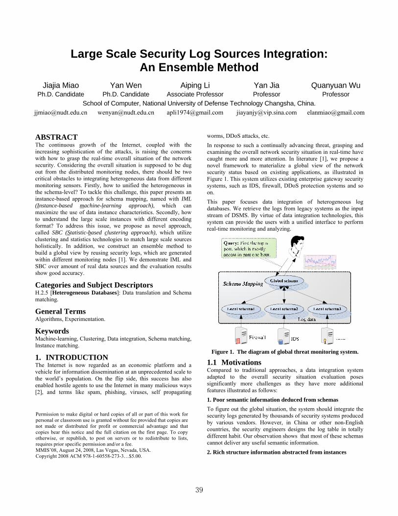
Large Scale Security Log Sources Integration: An Ensemble Method

Jiajia Miao Yan Wen Aiping Li Yan Jia Quanyuan Wu Ph.D. Candidate Ph.D. Candidate Associate Professor Professor Professor

School of Computer, National University of Defense Technology Changsha, China. jjmiao@nudt.edu.cn wenyan@nudt.edu.cn apli1974@gmail.com jiayanjy@vip.sina.com elanmiao@gmail.com

ABSTRACT The continuous growth of the Internet, coupled with the increasing sophistication of the attacks, is raising the concerns with how to grasp the real-time overall situation of the network security. Considering the overall situation is supposed to be dug out from the distributed monitoring nodes, there should be two critical obstacles to integrating heterogeneous data from different monitoring sensors. Firstly, how to unified the heterogeneous in the schema-level? To tackle this challenge, this paper presents an instance-based approach for schema mapping, named with IML (Instance-based machine-learning approach), which can maximize the use of data instance characteristics. Secondly, how to understand the large scale instances with different encoding format? To address this issue, we propose as novel approach, called SBC (Statistic-based clustering approach), which utilize clustering and statistics technologies to match large scale sources holistically. In addition, we construct an ensemble method to build a global view by reusing security logs, which are generated within different monitoring nodes [1]. We demonstrate IML and SBC over amount of real data sources and the evaluation results show good accuracy.

Categories and Subject Descriptors H.2.5 [Heterogeneous Databases]: Data translation and Schema matching.

General Terms Algorithms, Experimentation.

Keywords Machine-learning, Clustering, Data integration, Schema matching, Instance matching.

1. INTRODUCTION The Internet is now regarded as an economic platform and a vehicle for information dissemination at an unprecedented scale to the world’s population. On the flip side, this success has also enabled hostile agents to use the Internet in many malicious ways [2], and terms like spam, phishing, viruses, self propagating

worms, DDoS attacks, etc. In response to such a continually advancing threat, grasping and examining the overall network security situation in real-time have caught more and more attention. In literature [1], we propose a novel framework to materialize a global view of the network security status based on existing applications, as illustrated in Figure 1. This system utilizes existing enterprise gateway security systems, such as IDS, firewall, DDoS protection systems and so on. This paper focuses data integration of heterogeneous log databases. We retrieve the logs from legacy systems as the input stream of DSMS. By virtue of data integration technologies, this system can provide the users with a unified interface to perform real-time monitoring and analyzing.

Figure 1. The diagram of global threat monitoring system.

1.1 Motivations Compared to traditional approaches, a data integration system adapted to the overall security situation evaluation poses significantly more challenges as they have more additional features illustrated as follows: 1. Poor semantic information deduced from schemas

Permission to make digital or hard copies of all or part of this work for personal or classroom use is granted without fee provided that copies are not made or distributed for profit or commercial advantage and that copies bear this notice and the full citation on the first page. To copy otherwise, or republish, to post on servers or to redistribute to lists, requires prior specific permission and/or a fee. MMIS’08, August 24, 2008, Las Vegas, Nevada, USA. Copyright 2008 ACM 978-1-60558-273-3…$5.00.

To figure out the global situation, the system should integrate the security logs generated by thousands of security systems produced by various vendors. However, in China or other non-English countries, the security engineers designs the log table in totally different habit. Our observation shows that most of these schemas cannot deliver any useful semantic information. 2. Rich structure information abstracted from instances

39

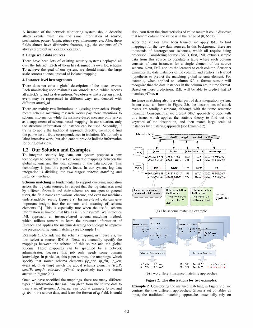
A instance of the network monitoring system should describe attack events must have the same information of source, destination, packet length, attack type, timestamp, etc. Also, these fields almost have distinctive features, e.g., the contents of IP always represent as ‘xxx.xxx.xxx.xxx’. 3. Large scale data sources There have been lots of existing security systems deployed all over the Internet. Each of them has designed its own log schema. To achieve the goal of our system, we should match the large scale sources at once, instead of isolated mapping. 4. Instance-level heterogeneous There does not exist a global description of the attack events. Each monitoring node maintains an ‘attack’ table, which records all attack’s id and its descriptions. We observe that a certain attack event may be represented in different ways and denoted with different attack_id. There are mainly two limitations in existing approaches. Firstly, recent schema matching research works pay more attentions to schema information while the instance-based measure only serves as a supplement of schema-based mapping. In our situation, only the structure information of instance can be used. Secondly, if trying to apply the traditional approach directly, we should find the pair-wise attribute correspondences in isolation. It’s not only a labor-intensive work, but also cannot provide holistic information for our global view.

1.2 Our Solution and Examples To integrate security log data, our system propose a new technology to construct a set of semantic mappings between the global schema and the local schemas of the data sources. This technology is just this paper’s focus. In our system, log data integration is dividing into two stages: schema matching and instance matching. Schema matching is fundamental to support querying mediation across the log data sources. In respect that the log databases used by different firewalls and their schema are not open to general users, the field names are various, obscure, and even not machine-understandable (seeing figure 2.a). Instance-level data can give important insight into the contents and meaning of schema elements [3]. This is especially true when the useful schema information is limited, just like as is in our system. We introduce IML approach, an instance-based schema matching method, which utilizes sensors to learn the structure information of instance and applies the machine-learning technology to improve the precision of schema matching (see Example 1). Example 1. Considering the schema mapping in Figure 2.a, we first select a source, IDS A. Next, we manually specify the mappings between the schema of this source and the global schema. These mappings can be specified by a network administrator, because this job only needs some domain knowledge. In particular, this paper suppose the mappings, which specify that source schema elements (ip_src, ip_dst, ip_len, event_id, timestamp) match the global schema elements (srcIP, destIP, length, attacked, pTime) respectively (see the dotted arrows in Figure 2.a). Once we have specified the mappings, there are many different types of information that IML can glean from the source data to train a set of sensors. A learner can look at example ip_src and ip_dst in the source data, and learn the format of ip field. It could

also learn from the characteristics of value range: it could discover that length column the value is in the range of [0, 65535]. After the sensors have been trained, we apply IML to find mappings for the new data sources. In this background, there are thousands of heterogeneous schemas, which all require being processed. Considering source IDS B, first, IML extracts sample data from this source to populate a table where each column consists of data instances for a single element of the source schema. Next, IML applies the learners to each column. Sensor A examines the data instances of the column, and applies its learned hypothesis to predict the matching global schema element. For example, when applied to column SJ, a format sensor will recognize that the data instances in the column are in time format. Based on these predictions, IML will be able to predict that SJ matches pTime.

Instance matching also is a vital part of data integration system. In our case, as shown in Figure 2.b, the descriptions of attack events are totally discrepant, although with the same semantic meaning. Consequently, we present SBC approach to cope with this issue, which applies the statistic theory to find out the keyword of the description, and then match large scale of instances by clustering approach (see Example 2).

(a) The schema matching example

(b) Two different instance matching approaches

Figure 2. The illustrations for two examples. Example 2. Considering the instance matching in Figure 2.b, we contrast the two different approaches. Given a set of tables as input, the traditional matching approaches essentially rely on

40

finding pair-wise tuple correspondence (e.g. ‘SYN Flood’ in Source S1 maps to ‘TCP SYN Flood Attack, belongs to Flood DDoS.’ in S2). In contrast, our approach considers the input tables holistically. These large scale source tables will give more information than pair-wise approach. Here we observe two distinguishing characteristics that offer a new view for instance-level matching: On one hand, we observe that there is a key word, which must be unique in the whole table. For example, ‘SYN’ is unique in one tuple, and then we use ‘SYN’ as a key word of this tuple. Also the key word can be summed up the meaning of this statement. On the other hand, there is large scale of data source, and we must match many instances at the same time and find all matchings at once. These dual observations motivate us to develop a statistical and holistic method to solve this problem. Specifically, first we search the keyword of each tuple, which is called generalizing stage. In this stage, we calculate the occurrence number of each word in one table, and then cut those words with high frequency. Second, unlike traditional approaches using pair-wise correspondence, we will consider the data sources together to define the global attack description. This should make the descriptions have more representativeness.

1.3 Contributions Compared to existing approaches, our approach makes three unique contributions. 1. We utilize a multi-strategy learning technology to find the semantic mappings based on source instances. Considering the special fields of ‘ip_src’ and ‘ip_dst’, this learning approach cannot distinguish the source from the destination. We design a statistics learner to tackle this problem. 2. We propose a novel framework to deal with the instance heterogeneous. Different from the traditional approaches, this framework matches the tuples holistically. 3. Finally, we validate the effectiveness of our framework over the real world applications. The results show that IML and SBC already obtain high accuracy. The paper is organized as follows. The next section reviews related work. Section 3 defines the matching problems. Sections 4-5 describe the whole integration system by present IML and SBC approaches. Section 6 presents our experiments. The last section discusses the future work and concludes.

2. Related Works Schema matching and instance matching are critical steps for schema integration [4][5]. We relate our work to existing works in these two aspects. Schema matching: Work on schema matching can be classified into schema-based and instance-based approaches. (For a comprehensive survey on schema matching, see [6][7].) In the instance-based approach, the Semint system [3] uses a neural-network learner. It matches schema elements using properties such as field specification (e.g., data types and scale) and statistics of data content (e.g., maximum, minimum, and average). The LSD [8] system, exploit other types of data information such as word frequencies and field formats. It utilizes both schema and data from the sources, and employs machine learning techniques to build the semantic mappings. The ILA system [9] matches schemas of two sources based on comparing objects that it knows to be the same in both sources. The DELTA [10] system

associates with each attribute a text string that consists of all metadata on the attribute, then matches attributes based on the similarity of the text strings. Our IML approach was motivated by LSD system and Semint system, which we also employ machine learning techniques and matches schema elements using properties such as statistics of data content and field formats. Instance matching: This problem is related to data exchange, which is the task of restructuring data from a source format (or schema) into a target format (or schema). The Clio system [11][12] introduces value correspondences, which specify functional relationships among related elements (e.g., hotel-tax = room-rate * state-tax-rate). Given a set of such correspondences, Clio produces the SQL queries that translate data from one source to the other. Clio explores joining elements along foreign keys, thus many possible ways to join. Toward the large scale matching, the closest idea is probably proposed by Bin et al. [13][14], they proposes a different approach, motivated by integrating large numbers of data sources on the Internet. First, a general statistical framework MGS for such hidden model discovery, which consists of hypothesis modeling, generation, and selection. Further, they specialized the general framework to develop algorithm MGSsd, targeting at synonym discovery, a canonical problem of schema matching, by designing and discovering a model that specifically captures synonym attributes.

Consequently, SBC approach cope with instance matching problem, which applies the statistic theory to find out the keyword of each attack event description, and then match large scale of instances by clustering approach (see Example 2).

3. Problem definition 3.1 Schema Matching The goal of schema mapping is to produce semantic mappings that enable the query based on the global schema. The focus of our work is to compute 1-1 mappings between the global schema and local source schemas. There are no more complex mappings in our project background. Also the input to the schema mapping problem is already structured data. We have discussed the data extraction phase of our global monitoring system in refer [1], which also benefiting from machine learning chniqute es. Given the schema names as distinct labels , , … , . Classification proceeds by training a Sensor on a set of training examples , , … , , , where is an object and is the observed label of that object. During the training phase, the sensor inspects the training examples and builds an internal classification model on how to classify objects. In the matching phase, given an object the sensor uses its internal classification model to predict label for . In this paper, we assume the prediction is of the form | , , … , | , , where ∑ | , 1, and | , is the confidence score of Sensor that matches label . The higher a confidence score, the more certain the sensor’s prediction is.

3.2 Instance Matching Each legacy security system has an attack description table, as shown in Figure 2.b. There are seemingly distinct tuples which represent the same real-world entity. In our global monitoring

41

system, we should find the correlations between t tables, and then we could translate the attack_id o rd.

differen t a single standa

Given the different tables of attack description , … , . Which consist of set of tuples, denoted by , … , , where

, . For each unique description , our task is output | .

4. The IML approach This section will describe IML in detail. IML operates in two phases: training and matching (see Figure 3). And there consists of four major components: sensor, combiner, scorer and manual intervention.

Figure 3. The two phase of IML approach. In the training phase, user prepares the samples for sensor to learn the value characteristic. Then, it trains the combiner how to assign the weight to each sensor. The output of the training phase is the internal classification models, for example prediction model[15]. In the matching phase, the trained sensors are used to match new source instance. The scorer will combine the sensors’ predictions. The output is mapping for the target schema. Users can either accept the mapping or provide some feedbacks.

4.1 The Training Phase 4.1.1 Data preparation Given several sources as input, IML begins with asking the user to specify 1-1 mappings between the global schema and the schema of these sources. Furthermore, after a new source has been matched by IML, it can serve as an additional training source. This makes IML unique that it can directly reuse past mappings to improve its performance. Next, user extracts data from the two sources for training. Following example 1, suppose that IML is given two sources IDS A and IDS B, whose schemas are shown in Figure 4.a, together with the global schema. Next user simply has to specify the mapping shown in Figure 4.b. And then the system extracts the samples of data stream per 5 seconds (see Figure 4.c)

4.1.2 Train the Sensors IML trains each sensor on the training samples. Each sensor will examine its training examples to construct an internal classification model that helps in matching the new sources. These models are part of the output of the training phase. In our system, there is totally four types sensor explained as follows:

Format Sensor: The format of value can represent as a Regular Expression, for instance, the IP value like ‘192.168.0.1’, which can be represented as ‘x.x.x.x’. Value Range Sensor: Range is one of the characteristics for those objects whose data types are number. For example, the value of Length field is [1, 65535]. Type Sensor: The special type will be presented in one table, e.g., time type in log table. Statistics Sensor: This sensor can catch the distribution of the data values. Our system is flexible enough, that user can define other sensors to extend IML.

4.1.3 Train the combiner The combiner uses a technique called stacking [16][17] to combine the predictions of sensors. Training the combiner works in the following steps [16]. Firstly, the combiner asks the sensors to predict the labels of the training examples. Secondly, since he combiner knows the correct result, it is able to judge how well each sensor performs with respect to each label. Finally, combiner assigns to each label and sensor a weight that indicates how much it trusts the predictions of sensor .

4.2 The Matching Phase Once the sensors and combiner have been trained, IML is ready to predict semantic mappings for new sources. Figure 5 illustrates the matching process on source IDS C. We describe the steps of this process in detail. Firstly, IML extracts a set of log data from IDS C (listing in Figure 5). Secondly, to match a source field, such as source, IML begin by matching each data instance of this field. IML applies the sensors to mach each instance, and then combine their predictions using the combiner. Thirdly, the combiner then combines the different predictions into a single prediction. For each filed, the scorer computes a combined score, which is the sum of the scores that the sensor give to that field, weighted by the sensor weights. Finally, according to the scores, our system takes these predictions together, and outputs the 1-1 mappings. As shown in Figure 5, users’ feedbacks can further improve matching accuracy, and is also necessary for matching the ambiguous schema elements. Sometimes the machine cannot precisely determinate the mapping relationship, then the user can intervene it. And this will do better for the situation come next time. Our framework enables easy and seamless integration of such feedback into the matching process.

5. The SBC approach We now describe SBC in detail. It operates in two phase: generalizing and clustering. In the generalizing phase, SBC should compute the weightiness of each word in the description field, and then cut the lower ones, which do not matter to understand the tuples. In other words, the remained words are the key words of the each tuple. In the clustering phase, different from the traditional matching approaches, SBC matching the entire input table at one time. We use a clustering method to find the correlations. Firstly, we cluster the semantic related descriptions together, and then the mapping of different ID should emerge naturally. Also, the entire matching of large scale tables should benefit that we should select the most representative of words for each attack description.

42

Figure 4. An example of the training phase.

5.1 The Generalizing Phase There is a premise that we must take into account. The weightiness of terms in each tuple is not equal to each other. In fact, the key word is usually the one which does not occurs in other descriptions, i.e., as shown in figure 2.a, the word ‘This’ occur two time in two tuples, and ‘DDoS’ is unique in the whole table of description field. According to this observation, the frequency of the word is negative correlation with the importance of word. This relies on their information entropy [18]. For implementation, we splice all description of a certain table as a paragraph. Then we calculate the weightiness of each distinct term to select the keyword. The following formula defines i-th term’s information entropy, · . Where / .

denotes the sum number of terms in this paragraph. denotes the sum of the occur time of the certain term. In addition, the weightiness of term is defined as follows, ∑ .

Then we could get the keyword of each tuple in one table, according to the weightiness of terms. We should promise that there exists at least one word to represent one tuple.

5.2 The Clustering Phase Once the generalizing is finished, SBC takes the processed tables as input, and matching all the tuples holistically. We consider matching the tuples in a clustering approach (see Figure 7). Because the data is so simple that we just use the standard

clustering algorithm [19][20] to finish this job. In figure 7, , represents the distance that between object[i] and cluster[j], and denotes the threshold that the SBC designed. The number of objects with a cluster[j] is denoted as member[j].

Figure 5. An example of the matching phase.

Fast Standard Clustering Algorithm Input: object[N]: array of data objects Output: cluster[K]: array of cluster centers 1: K=0; 2: N=number of objects; 3: For i=0 t N-o 1

0 to k If

4: For j=5: , then 6: object[i] belong to cluster[j]; 7: member[j]++; 8: newCluster=false; 9: If newCluster then 10: createCluster(object[i]); 11: member[j]=0; 12: K++; 13: Output cluster[K];

Figure 7. The fast standard clustering algorithm for large scale instance matching.

After the clustering algorithm, SBC finds out the high score of member[j], which means that these terms are frequently used by

43

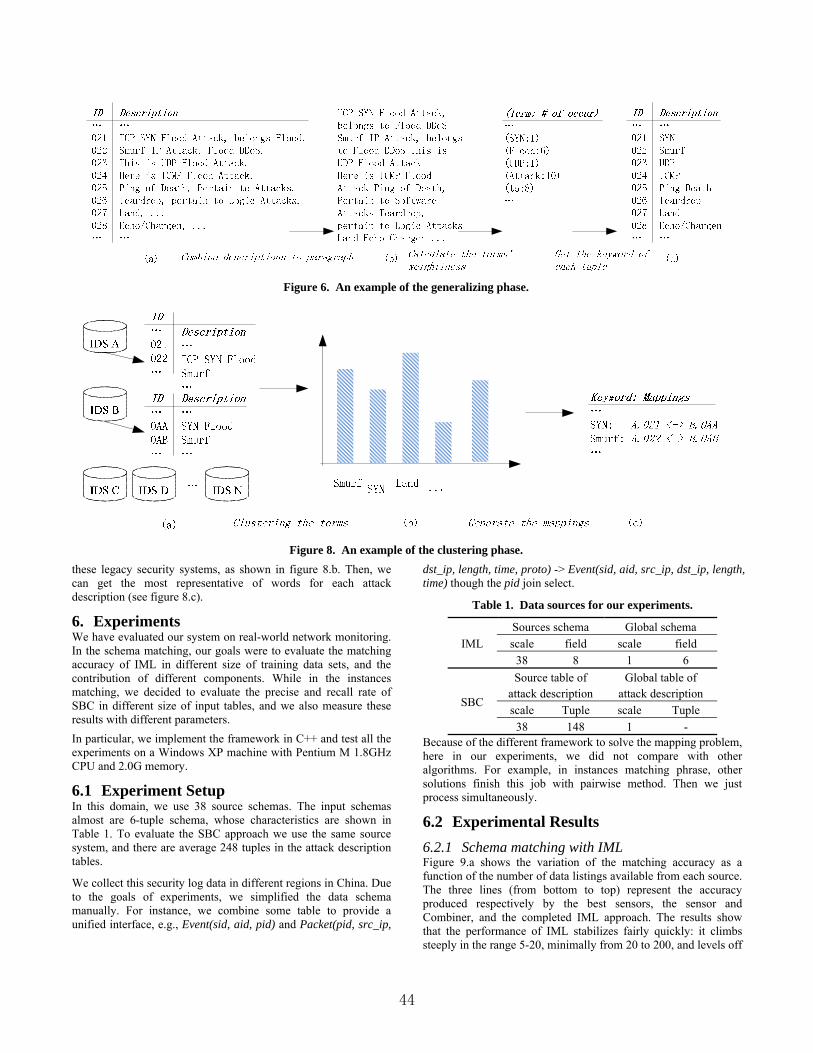
Figure 6. An example of the generalizing phase.

these legacy security systems, as shown in figure 8.b. Then, we can get the most representative of words for each attack description (see figure 8.c).

6. Experiments We have evaluated our system on real-world network monitoring. In the schema matching, our goals were to evaluate the matching accuracy of IML in different size of training data sets, and the contribution of different components. While in the instances matching, we decided to evaluate the precise and recall rate of SBC in different size of input tables, and we also measure these results with different parameters. In particular, we implement the framework in C++ and test all the experiments on a Windows XP machine with Pentium M 1.8GHz CPU and 2.0G memory.

6.1 Experiment Setup In this domain, we use 38 source schemas. The input schemas almost are 6-tuple schema, whose characteristics are shown in Table 1. To evaluate the SBC approach we use the same source system, and there are average 248 tuples in the attack description tables.

We collect this security log data in different regions in China. Due to the goals of experiments, we simplified the data schema manually. For instance, we combine some table to provide a unified interface, e.g., Event(sid, aid, pid) and Packet(pid, src_ip,

dst_ip, length, time, proto) -> Event(sid, aid, src_ip, dst_ip, length, time) though the pid join select.

Figure 8. An example of the clustering phase.

Table 1. Data sources for our experiments.

IML Sources schema Global schema scale field scale field 38 8 1 6

SBC

Source table of attack description

Global table of attack description

scale Tuple scale Tuple 38 148 1 -

Because of the different framework to solve the mapping problem, here in our experiments, we did not compare with other algorithms. For example, in instances matching phrase, other solutions finish this job with pairwise method. Then we just process simultaneously.

6.2 Experimental Results 6.2.1 Schema matching with IML Figure 9.a shows the variation of the matching accuracy as a function of the number of data listings available from each source. The three lines (from bottom to top) represent the accuracy produced respectively by the best sensors, the sensor and Combiner, and the completed IML approach. The results show that the performance of IML stabilizes fairly quickly: it climbs steeply in the range 5-20, minimally from 20 to 200, and levels off

44

after 200. IML thus appears to be robust, and can work well with relatively little data.

0 100 200 300 400 5000

10

20

30

40

50

60

70

80

90

100

Mat

chin

g ac

cura

cy (%

)

Number of data samples per source

Sensors Sensors + Combiner Sensors + Combiner + user feedback

(a) Matching accuracy of different sample scale

0 100 200 300 400 5000

10

20

30

40

50

60

70

80

90

100

Mat

chin

g ac

cura

cy (%

)

Number of data samples per source

IML without Format Senor IML without Value Range Senor IML without Type Senor IML without Combiner The complete IML system

(b) Matching accuracy without some components

Figure 9. The results of experiments with IML approach. As shown in Figure 9.b, the contribution of sensors and combiner are indispensability. The first line (from top to bottom), represents the accuracy produced by IML. The second line denotes that IML without combiner, and the 3-5th lines represent the IML without a sensor. Without sensors or combiner, the accuracy of IML charges downslide clearly. The results show that with the current system, both sensors and combiner make important contributions to the overall performance.

6.2.2 Instance matching with SBC As description in Section 5, the parameters of the generalizing and clustering phrase, these have great influence on the precision and recall of experimental results. Here, denotes the number of terms we select as keyword candidates in the generalizing phrase, and represents the distance threshold when we clustering the semantic related keywords. The parameters are set by our experience. Figure 10.a shows the different precision with different parameters setting. The x-axis represents the different value-pair ( , ), and the y-axis denotes the precision of SBC approach. For each scale, the four bars (from left to right)

represent the different scales of matching table. Figure 10.b shows the different recall with different parameters setting. The coordinate axes represent the same meanings as Figure 10.a. We can also discover that the precision and recall of SBC is strongly related to the parameters values and input tables’ scale. We will discuss the adaptive feature in future work of section 7.

According to o onment, we design ur data envir , 0.3,200 , 0.5,200 , 0.7,200 , 0.3,300 , 0.5,300 , 0.7,300. As shown in Figure 10, the keywords should decrease with the increasing of , and this will induce that, the precision of SBC should decrease, while the recall of SBC should synchronized grow up. Due to the increase of , the number of cluster decrease.

(0.3,200) (0.5,200) (0.7,200) (0.3,300) (0.5,300) (0.7,300)0

50

60

70

80

90

100

Pre

cisi

on (%

)

(&distance,Nterms)

12 sources 25 sources 38 sources

(a) The precision of SBC with different data scale and parameters

(0.3,200) (0.5,200) (0.7,200) (0.3,300) (0.5,300) (0.7,300)0

50

60

70

80

90

100

Rec

all (

%)

(&distance,Nterms)

12 sources 25 sources 38 sources

(b) The recall of SBC with different data scale and parameters

Figure 10. The results of experiments with SBC approach.

7. Conclusions and future works For the security log integration, we split the problem into two aspects: schema matching and instance matching. We have described an approach to schema matching that employs and extends machine learning techniques. Also we present a novel

45

approach to instance matching, which utilize the statistics information and clustering algorithm. In schema matching aspect, due to the special situation, we focus the instance-based measure method. The system applies sensors, each of which looks at the problem from a different perspective, then combines the sensors’ predictions. Our system also utilized user feedback to improve the accuracy. Finally, experiment show IML appears to be robust and efficient. In instance matching aspect, we consider handling large scale tables together. This is different from the traditional approach, which though the pair-wise matching. The large scale tables could provide enough information for us to select the most representative of words for each attack description. Also, the clustering algorithm should become more precise with the large scale data. The experiment results verify SBC is efficient enough. Next, we will extend our current work in three ways. First, we should address the n:m mapping problem, which exists in data integration system commonly. Second, we should develop more sensors to grasp other different characteristics of data values. Finally, we must improve our clustering algorithm to tune parameters. From the experiments, we have aware that this will make our approach more robust.

Acknowledgment: We thank Chen Yingwen for providing valuable comments on our paper. We also thank Wang Le, Du Kai, Tian Li, Yuan Zhijian for their useful suggestions. This paper is supported by the National High-Tech Research and Development Plan of China ("863" plan) under Grant No. 2006AA01Z451 and No. 2007AA01Z474, and Program for New Century Excellent Talents in University (NCET-06-0928).

8. REFERENCES [1] Jiajia Miao, “GS-TMS: A Global Stream-based Threat

Monitor System,” Proceedings of the 34st international conference on Very large data bases, PhD Workshop, New Zealand: 2008.

[2] US-CERT, “Technical Cyber Security Alerts”; http://www.us-cert.gov/cas/techalerts/.

[3] W. [Reference to Li] and C. [Reference to Clifton], “SEMINT: A tool for identifying attribute correspondences in heterogeneous databases using neural networks,” Data & Knowledge Engineering, vol. 33, Apr. 2000, pp. 49-84.

[4] C. Batini, M. Lenzerini, and S.B. Navathe, “A comparative analysis of methodologies for database schema integration,” ACM Comput. Surv., vol. 18, 1986, pp. 323-364.

[5] L.J. Seligman et al., “Data Integration: Where Does the Time Go?” IEEE Data Engineering Bulletin, vol. 25, 2002, pp. 3-10.

[6] A. Doan and A.Y. Halevy, “Semantic-integration research in the database community,” AI Mag., vol. 26, 2005, pp. 83-94.

[7] E. Rahm and P.A. Bernstein, “A survey of approaches to automatic schema matching,” The VLDB Journal The International Journal on Very Large Data Bases, vol. 10, Dec. 2001, pp. 334-350.

[8] A. Doan, P. Domingos, and A.Y. Halevy, “Reconciling schemas of disparate data sources: a machine-learning approach,” Proceedings of the 2001 ACM SIGMOD international conference on Management of data, Santa Barbara, California, United States: ACM, 2001, pp. 509-520.

[9] M. Perkowitz and O. Etzioni, “Category translation: Learning to understand information on the internet,” Proc. of Int. Joint Conf. on AI (IJCAI), 1995.

[10] C. Clifton, E. Housman, and A. Rosenthal, “Experience with a combined approach to attribute-matching across heterogeneous databases,” Proc. of the IFIP Working Conference on Data Semantics (DS-7), 1997.

[11] R.J. Miller et al., “The Clio project: managing heterogeneity,” SIGMOD Rec., vol. 30, 2001, pp. 78-83.

[12] L.M. Haas et al., “Clio grows up: from research prototype to industrial tool,” Proceedings of the 2005 ACM SIGMOD international conference on Management of data, Baltimore, Maryland: ACM, 2005, pp. 805-810.

[13] B. He, K.C. Chang, and J. Han, “Discovering complex matchings across web query interfaces: a correlation mining approach,” Proceedings of the tenth ACM SIGKDD international conference on Knowledge discovery and data mining, Seattle, WA, USA: ACM, 2004, pp. 148-157.

[14] B. He and K.C. Chang, “Making holistic schema matching robust: an ensemble approach,” Proceedings of the eleventh ACM SIGKDD international conference on Knowledge discovery in data mining, Chicago, Illinois, USA: ACM, 2005, pp. 429-438.

[15] Q. Yang, H.H. Zhang, and T. Li, “Mining web logs for prediction models in WWW caching and prefetching,” Proceedings of the seventh ACM SIGKDD international conference on Knowledge discovery and data mining, San Francisco, California: ACM, 2001, pp. 473-478.

[16] K.M. Ting and I.H. Witten, “Issues in stacked generalization,” J ARTIF INTELL RES, vol. 10, 1999, pp. 271-289.

[17] D.H. Wolpert, “Stacked generalization,” Neural Networks, vol. 5, 1992, pp. 241-259.

[18] A. Daemi and J. Calmet, “From Ontologies to Trust through Entropy,” Proceedings of the International Conference on Advances in Intelligent System, Luxembourg, 2004.

[19] P. Berkhin, “A Survey of Clustering Data Mining Techniques,” Grouping Multidimensional Data, 2006, pp. 25-71.

[20] R. Xu and D. Wunsch, “Survey of clustering algorithms,” IEEE Transactions on Neural Networks, vol. 16, 2005, pp. 645-678.

46

APPLYING MDA TO INTEGRATE MINING TECHNIQUES INTO DATA WAREHOUSES: A TIME SERIES CASE STUDY

Jesús Pardillo Dep. of Software and Computing Systems

University of Alicante, Spain

jesuspv@dlsi.ua.es

Jose Zubcoff Dep. of Sea Sciences and Applied Biology

University of Alicante, Spain

Jose.Zubcoff@ua.es

Jose-Norberto Mazón Dep. of Software and Computing Systems

University of Alicante, Spain

jnmazon@dlsi.ua.es

Juan Trujillo Dep. of Software and Computing Systems

University of Alicante, Spain

jtrujillo@dlsi.ua.es

ABSTRACT Data mining is one of the most important analysis techniques to automatically extract knowledge from large amount of data. Nowadays, data mining is based on low-level specifications of the employed techniques typically bounded to a specific analysis platform. Therefore, data mining lacks a modelling architecture that allows analysts to consider it as a truly software-engineering process. Bearing in mind this situation, we propose a model-driven approach which is based on (i) a conceptual modelling framework for data mining, and (ii) a set of model transformations to automatically generate both the data under analysis (that is deployed via data-warehousing technology) and the analysis models for data mining (tailored to a specific platform). Thus, analysts can concentrate on understanding the analysis problem via conceptual data-mining models instead of wasting efforts on low-level programming tasks related to the underlying-platform technical details. These tasks are now entrusted to the model-transformations scaffolding. The feasibility of our approach is shown by means of a hypothetical data-mining scenario where a time series analysis is required.

Categories and Subject Descriptors D.2.1 [Software Engineering]: Requirements/Specifications – elicitation methods, languages, tools

D.2.12 [Software Engineering]: Interoperability – data mapping, interface definition languages.

D.2.13 [Software Engineering]: Reusable Software – domain engineering, reusable models.

H.2.3 [Database Management]: Languages – query languages, data description languages (DDL), data manipulation languages (DML). H.2.8 [Database Management]: Database Applications – data mining.

General Terms Management, Documentation, Design, Standardization, Languages.

Keywords data mining, data warehouse, model-driven engineering, model transformation, multidimensional modelling, conceptual modeling

1. INTRODUCTION Data-mining techniques allow analysts to discover knowledge (e.g., patterns and trends) in very large and heterogeneous data sets. Data mining is a highly complex task which requires a great effort in preprocessing data under analysis, e.g., data exploration, cleansing, and integration [22]. Therefore, some authors suggest the suitability of data-warehousing technologies [6] for improving the conventional knowledge discovery in databases process [7,8] by means of providing an integrated and cleansed collection of data over which data-mining techniques can be straight applied [5,23]. However, the current data-mining literature has been focused on the presenting new techniques and improving the underlying algorithms [4], whilst the most known software platforms do not apply the data-warehousing principles during the data-mining design. To overcome this situation, several mechanisms have been proposed [26,27,28,20] to model data-mining techniques in conjunction with data-warehousing technology from the early stages of design (i.e., at the conceptual level). These data-mining models do not only support analysts in using and understanding the required data-mining techniques in real-life scenarios, but also allow designers to document the data-mining techniques in detail. Hence, these data-mining models are truly blueprints that can be used to manually obtain the required data-mining metadata as a basis of the implementation in a certain data-mining platform. However, this highly-complex task is only accessible to expert analysts and requires too much effort to be successfully completed [5,9].

Permission to make digital or hard copies of all or part of this work for personal or classroom use is granted without fee provided that copies are not made or distributed for profit or commercial advantage and that copies bear this notice and the full citation on the first page. To copy otherwise, or republish, to post on servers or to redistribute to lists, requires prior specific permission and/or a fee.

In this work, we will go beyond the definition of new models, here we define a model-driven engineering [1] approach for data mining. Moreover, we propose the use of a well-known visual modeling standard, the “unified modelling language” (UML) [17]

Conference’04, Month 1–2, 2004, City, State, Country. Copyright 2004 ACM 1-58113-000-0/00/0004…$5.00.

47

Table 1. Comparison of data-mining modelling languages

Language CDM CWM XELOPES DMX Weka

Type metamodel metamodel library query language library Technology UML profiles MOF instance CWM extension SQL-like computation

Subject interaction interoperability interoperability

computation querying computation

Abstraction high middle middle low low Complexity low medium high medium high User type analysts data managers data managers data miners data miners Expertise low medium high medium high

for facilitating thedesign and implementation tasks. In order to spread the usage of data-mining models to a broader scope of analysts and reduce the required effort our approach automatically generate a vendor-specific data-mining implementation from a conceptual data-mining model, taking into consideration the deployment of the underneath data warehouse (i.e., data under analysis). The rest of the paper is structured as follows: the next Section outlines the related work. Section 3 describes our model-engineering approach for data mining by describing (i) the modelling solution and (ii) the proposed model-transformation architecture. For this aim, a case study is used through the paper to clarify every theoretical detail. Finally, Section 4 exposes conclusions, also sketching the ongoing work.

2. RELATED WORK Current approaches for data-mining can be classified on those that are a general description of data-mining process, or mathematical oriented, and propose solutions at a highly low-abstraction level. However, both approaches overlook the definition of understandable artifacts that could be easily used by designers in a software engineering process. The main standard proposed for the data mining process is the “cross industry standard process for data mining” [2]. This standard is a detailed description of each of the six phases of the data-mining process. Nevertheless, this standard neither proposes a concrete modeling tool nor presents a conceptual model for data mining. CRISP-DM is focused on the description of how to perform a data-mining task, and thus, it remains as a high-level definition of the data-mining process. The six phases of CRISP-DM are: business understanding, data understanding, data preparation, modeling (i.e., as a selection of data and algorithm for the specific goal)1, evaluation, and deployment. Each one of these phases is dependent of the previous one: data understanding requires a good comprehension of the business. Then, this standard defines the main aspects to be considered in each of the six phases. However, CRISP-DM does not propose any artifacts, platform or language for modeling data mining. An overview of current data-mining modelling languages is provided in Table 1. The “common warehouse metamodel” (CWM) [17] and the “predictive model markup language”

1 In CRISP-DM, the word modeling is used as selecting the required data and algorithm to perform the data mining task.

(PMML)2 [3] are really standards for the metadata interchange proposed by vendor-independent consortiums (OMG and DMG, respectively) between data-mining applications based on XML, but they cannot be used as analysis artifacts. The “data mining extensions” (DMX) [16] is a SQL-like language for (textually) coding data-mining models in the Microsoft Analysis Services platform, and therefore it is difficult to gain understanding of the data-mining domain. In addition, some data-mining libraries have been also proposed as a modelling mechanism. Two of the most known are the “extended library for Prudsys embedded solutions” (XELOPES) [21] (derived from CWM) and Weka [25]. They provide an entire framework to carry out data mining but, once again, they are situated at very low-abstraction level, since they are code-oriented and they do not contribute to facilitate understanding of the domain problem. On the other hand, there are software architectures related to data mining such as the “pattern-base management system” (PBMS) [24] designed to store and manage patterns obtained from the usage of data-mining techniques, but they cannot be considered a truly modelling proposal as we state herein. All of these approaches have the same drawback, since they are focused on solving the technical scaffolding instead of providing analysts with intuitive artifacts to specify data mining. To the best of our knowledge, only the proposal described in [26-28,20] provides a modelling framework (CDM in Table 1) to define data-mining techniques at a high-abstraction level by using the “unified modelling language” (UML) [17]. However, these UML-based models are mainly used as documentation. In this paper, we propose to extend this modelling framework as a first step in turning data mining into a real software engineering process. Specifically, we use model-driven engineering concepts to (i) specify data-mining analysis in two technology-independent models (the multidimensional-data model of the underlying data warehouse and the data mining technique model), and (ii) provide transformations to automatically deploy data and analysis specifications into their physical implementations.

2 In Table 1, we exclude PMML due to the space constraints. PMML is simmilar to CWM but it is a language (Type field) coded in XML schema (Technology).

48

3. MODEL-DRIVEN ARCHITECTURE FOR DATA MINING IN DATA WAREHOUSES Our model-driven engineering approach for data mining advocates defining the underneath data warehouse (i.e., data under analysis) together with the corresponding data-mining technique. In this section, both tasks are explained, as well as the required transformations to obtain the data-mining implementation. In order to clarify the theoretical details that lay behind our solution, we employ a case study in the rest of the text.

3.1 MODELLING THE DATA UNDER ANALYSIS This section explains how to develop the underlying data warehouse required for data-mining to provide integrated and cleansed data. The data warehouse is based on a multidimensional model which defines the required data structures, namely facts and dimensions and their respective measures, hierarchies and attributes. Multidimensional modelling resembles the traditional database design [23]. First, a conceptual design phase is performed whose output is an implementation-independent and expressive conceptual multidimensional model for the data warehouse. A logical design phase then aims to obtain a technology-dependent model from the previously defined conceptual multidimensional model. This logical model is the basis for the implementation of the data warehouse. In previous work, we have aligned this process with a model-driven approach [19,18,11,12] in order to support designers to develop a conceptual multidimensional model and the automatic derivation

of its corresponding implementation. In Fig. 1, we show a conceptual data modelling example for mining the represented data. In this example, a small organisation is trying to highlight patterns and trends in the evolution of the fish-species population along time. For accomplishing this task, the data under analysis must be specified by exploring the underlying multidimensional data of the data warehouse that stores them. The conceptual model of Fig. 1 has been defined by using our UML profile for multidimensional modelling [10]. This

modelling paradigm that is implemented in our profile, enables designers to specify intuitive data models in terms of facts and dimensions of analysis that are employed to perform multidimensional analyses. Each fact contains several measures or fact attributes whose are described around several dimensions. On the other hand, each dimension represents an axis of analysis that is also described by means of several kinds of dimension attributes. In addition, typically, these dimensions contain hierarchies of aggregation that allow analysts to represent the factual data under different levels of detail or granularities. By using the multidimensional modelling, Fig. 1 shows the designed captures fact together with a set of four dimensions: fish, ship, time, and location. For each dimension, several levels are defined that form a hierarchy of aggregation. Locations have a <site, marine area, region> hierarchy, fish have a <species, genus, family> hierarchy, and the time dimension has the typical <day, week, month, quarter, year> hierarchy. Finally, ships have no hierarchies to be described, thus presenting only one aggregation level with data of the ship. From this conceptual model, an implementation of the required data structures can be automatically obtained tailored to several specific platforms, e.g., relational [15] or multidimensional [14].

3.2 MODELLING DATA MINING TECHNIQUES: THE TIME-SERIES ANALYSIS EXAMPLE On the other hand, after the phase of conceptual modelling the data under analysis we will be able to also design a conceptual model for applying a data-mining technique on the represented

data. Due to the requirements for data mining involved in our case study, we select its time-series analysis. Therefore, we apply our UML profile for time-series analysis presented in [20]. This profile enables data miners to carry out time-series analysis by means of representing the typical modelling elements of this kind of technique. By using this modelling framework, in Fig. 2, we show the resulting time-series modelling for our case study in order to forecast the total number of carps captured per month. Typically, this modelling implies the definition of data-mining

Figure 1. Multidimensional data modelling of the carp captures case study

49

settings (in this case, the “Carp Captures by Month”) that contains slots such as the periodicity one which can be set specific values for tunning the underlying data-mining algorithm. In addition, a data-mining technique is specified by means of modelling several data links to the underlying data warehouse and thus, to the presented multidimensional model (Fig. 1). For instance, for the time-series analysis in Fig. 2, we specify an input variable (the

individuals) that also acts as output of the requested forecasting. Together with this variable, additional data can be specified for filtering the input data, e.g., carp species, and importantly, the time granularity that is always required during a time-series analysis (months in the case study). It is worth noting that the our comprehensive modelling solution enable analysts to easily drive the data-mining process at the first stage of the data-mining proces in an intuitive way that also is independent of any data-mining platform.

3.3 TRANSFORMATIONS FOR MODEL-DRIVEN DATA MINING Whilst the derivation of the data under analysis is traditionally performed through a three-step process, analysis techniques such as data mining present different requirements for their development. In this section, a model-driven engineering approach for the deployment of data-mining models together with the data under analysis is described. The novelty of our approach is twofold: (i) it is based on defining vendor-neutral models of data-mining techniques together with the model of the underlying data warehouse, and (ii) the deployment of those data-mining techniques is done automatically. Therefore, on one hand, we use a modelling approach [26-28,20] for defining platform-independent models for several data-mining techniques. This approach is a high-level vendor-neutral modelling language to visually and easily specify analysis by means of applying data-mining techniques. On the other hand, this language is not directly implemented in any data-mining platform, and thus, it only acts as a blueprint of the executable analysis. Therefore, the model-transformation configuration has to be described in order to consider every kind of target platform from this platform-independent modelling language. In Fig. 3, we provide an overview of the required

model-transformation architecture, stressing some of the current data-mining standards and platforms in the market. The conceptual data-mining modelling framework in data warehouses [26-28,20] is shown at the top of this model-driven architecture. Fig. 3 also shows the transformation paths to derive several implementations through mapping data-mining models to other languages that really have established an executable

environment: CWM, XELOPES, DMX, or Weka acting as bridge. Depending to the characteristics of the analysis itself (e.g., the required technique) or the data-mining solution available (e.g., it can only be open-source platforms), we choose one of the transformation paths. Furthermore, Depending on the target-language representation, model-to-model or model-to-text transformations could be needed. Therefore, some of the data-mining solutions that are able to interpret the previous modelling languages are also represented in Fig. 3. On the lower side, some of the data-mining platforms are also represented. Whereas there are standards such as CWM that are vendor-neutral and many CWM-compliant tools can be considered (Oracle Miner3, CWM4ALL4, etc.), others such as DMX are commonly restricted to the platform for which they are originally were thought (the Microsoft’s in this case).

Figure 3. Model-transformation architecture for model-driven data mining Figure 2. Modelling time-series analysis on the

multidimensional data of carp captures

From a technical point of view, we propose the usage of the “model-driven architecture” (MDA) [17] in order to implement these transformations between data-mining models. Within an MDA-based approach the “query/view/transformation” (QVT) language can be used as a standard mechanism for defining formal relations between MOF-compliant models that allows the automatic derivation of a implementation. Nevertheless, there are transformations that are applied from models (i.e., MOF-based) to implement code (i.e., textual modelling languages). In these cases, MDA offers the “MOF models to text transformation” (Mof2Text) language that allows us to specify transformations by means of textual templates in order to automatically derive the corresponding implementation.

3 URL: www.oracle.com/technology/products/bi/odm (June 2008) 4 URL: www.cwd4all.com (June 2008)

50

Figure 4. Example of a Mof2Text transformation and the generated code

3.4 EXAMPLE DATA-MINING TRANSFORMATION FOR A SPECIFIC PLATFORM Herein, we follow our case study for carrying out a time-series analysis of fish-species population (see Fig. 2&3), in order to automatically derive the implementation for a specific software platform5. Specifically, in this paper, we employ the Microsoft Analysis Services6 as the target platform. As we previously shown, this platform provides the DMX language to code data-mining models. Therefore, given the time-series analysis model of Fig. 2, we have designed the required mapping from this model into DMX code. Due to the space constraints, we exclude an abstract specification of the involved mapping, also omitting an example transformation of the data under analysis that can be found in [11]. Nevertheless, in Fig. 4, it is shown the implementation of this mapping (left-hand side) over the Eclipse development platform. In order to accomplish this task, we have used the MOFScript7 plug-in for this platform. MOFScript is a transformation-language implementation of the Mof2Text standard language that enable us to specify model-to-text transformations in the “model-driven architecture” (MDA) [17] proposal. On the right-hand side, the resulting DMX code for the time-series analysis of Fig. 2 is shown. Given Fig. 4, the mapping overview is as follows: each time-series analysis (represented by some kind of modelling element in the source metamodel) is mapped into a data-mining model in DMX (MINING MODEL instruction). Every parameter of the analysis technique is also mapped into their DMX counterpart. In

5 We refer reader to [18,11] for a sample transformation of the data under analysis. 6 URL: www.microsoft.com/sql/solutions/bi (June 2008) 7 URL: www.eclipse.org/gmt/mofscript (June 2008)

addition, the unspecified parameters in the conceptual model are later explicitly defined in the implementing code. On the other hand, each data under analysis (taken from the multidimensional model of the underlying data warehouse) is mapped into a data-mining attribute in DMX (by defining a table and then creating its corresponding column). Once the mapping is correctly established, the MOFScript engine can interpret this one in order to translate a certain conceptual model of time-series analysis to the DMX code, and thus, implementing it in the Microsoft Analysis Services platform. Finally, within this solution, analysts can consult the data-mining results by visualising the obtained patterns and trends and extracting new knowledge from them.

4. CONCLUSIONS Due to mathematical foundations of data-mining techniques, there are no formalised mechanisms to easily specify data-mining activities as a real software engineering process. In this paper, we propose a model-engineering approach for overcoming this limitation. On one hand, we provide a set of models to specify data-mining techniques in an vendor-neutral way that are close to the way of analysts thinking about data-mining (i.e., conceptual models). On the other hand, we provide transformations to automatically derive platform-specific models from the conceptual ones, altogether with the deployment of data under analysis [11,14]. Thus, analysts can only focus on data mining itself at an abstract level instead of distracting by details related to a certain vendor data-mining solution whilst the model transformations can automatically derive vendor-specific implementations in background for current data-mining platforms. Furthermore, our approach for data-mining modelling is also concerned about modelling the data under analysis, i.e., the data warehouse in order to provide analysts with a way of quickly understand for being close to their way of thinking about data. The data-mining techniques are smoothly integrated in this model. Therefore, the great benefit of our approach is that, once we have established the model-driven architecture for both data under

51

analysis and analysis techniques for data mining, analysts can model their data-mining related tasks easily in a vendor-neutral way whereas the model-transformations scaffolding is entrusted to automatically implement them in a certain platform. Our ongoing work covers other high-level mechanisms to specify data-mining related tasks. For instance, we will study how current goal-oriented approaches for requirement analysis [12] can help us to guide the selection of data-mining solutions. In addition, we are investigating on the integration of the proposed data-mining framework together with the analysis technologies traditionally employed in the data-warehouse domain.

5. REFERENCES [1] Bézivin, J., 2006. Model Driven Engineering: An Emerging

Technical Space. GTTSE, pp. 36-64. [2] CRISP-DM Consortium, June 2008. CRISP-DM, version

1.0. http://www.crisp-dm.org. [3] Data Mining Group, June 2008. Predictive Model Markup

Language (PMML), version 3.2. http://www.dmg.org/pmml-v3-2.html.

[4] Hand, D.J., Mannila, H., Smyth, P., 2001. Principles of Data Mining. MIT Press.

[5] Inmon, W.H., 1996. The Data Warehouse and Data Mining. Commun. ACM, Vol. 49, No. 4, pp. 83–88.

[6] Kimball, R., Ross, M., 2002. The Data Warehouse Toolkit. Wiley.

[7] Frawley, W. J., Piatetsky-Shapiro, G., Matheus, C. J., 1991. Knowledge Discovery in Databases: An Overview. AAAI/MIT Press.

[8] Fayyad, U., Piatetsky-Shapiro, G., Snyth, P., Uthurusamy, R., 1991. Advances in knowledge discovery and data mining. AAAI/MIT Press.

[9] González-Aranda, P., Menasalvas, E., Millán, S. Segovia, J., 2004. Towards a Methodology for Data Mining Project Development: The Importance of abstraction. ICDM/FDM, pp. 39-46.

[10] Luján-Mora, S., Trujillo, J., Song, I.Y., 2006. A UML profile for multidimensional modeling in data warehouses. Data Knowl. Eng. Vol. 59, No. 3, pp. 725.769.

[11] Mazón, J.N., Trujillo, J., 2008. An MDA approach for the development of data warehouses. Dec. Support Syst. Vol. 5, No. 1, pp. 41-58.

[12] Mazón, J.N., Pardillo, J., Trujillo, J., 2007. A Model-Driven Goal-Oriented Requirement Engineering Approach for Data Warehouses. ER Workshops, pp. 255–264.

[13] Mazón, J.N., Trujillo, J., Lechtenbörger, J., 2007. Reconciling requirement-driven data warehouses with data sources via multidimensional normal forms. Data Knowl. Eng. Vol. 63, No. 3, pp. 725-751.

[14] Mazón, J.N., Pardillo, J., Trujillo, J., 2006. Applying Transformations to Model Driven Data Warehouses. DaWaK, pp. 13–22.

[15] Mazón, J.N., Trujillo, J., Serrano, M., Piattini, M., 2005. Applying MDA to the development of data warehouses. DOLAP. pp. 57-66.

[16] Microsoft, June 2008. Data Mining eXtensions (DMX). http://msdn2.microsoft.com/enus/library/ms132058(VS.90).aspx

[17] Object Management Group, June 2008. Common Warehouse Metamodel (CWM), Unified Modeling Language (UML), Model Driven Architecture (MDA), Query/View/Transformation Language (QVT), MOF Model to Text Transformation Language (Mof2Text). http://www.omg.org.

[18] Pardillo, J., Mazón, J.N., Trujillo, J., 2008. Model-driven Metadata for OLAP Cubes from the Conceptual Models of Data Warehouses. DaWaK. In Press.

[19] Pardillo, J., Trujillo, J., 2008. Integrated Development of Data Warehouses and Data Marts by Applying Model-driven and Goal-oriented Requirement Engineering. ER. In Press.

[20] Pardillo, J., Zubcoff, J., Trujillo, J., 2008. Un perfil UML para el análisis de series temporales con modelos conceptuales sobre almacenes de datos. IDEAS Workshop. pp. 369-374.

[21] Prudsys, June 2008. Extended Library for Prudsys Embedded Solutions (XELOPES). www.prudsys.com/Produkte/Algorithmen/Xelopes.

[22] Pyle, D., 1999. Data Preparation for Data Mining. Morgan Kaufmann.

[23] Rizzi, S., Abelló, A., Lechtenbörger, J., Trujillo, J., 2006. Research in data warehouse modeling and design: dead or alive? DOLAP, pp. 3-10.

[24] Theodoridis, Y., June 2008. Pattern-base Management System (PBMS). http://www.pbms.org.

[25] University of Waikato, June 2008. Weka. http://www.cs.waikato.ac.nz/ml/weka.

[26] Zubcoff, J., Pardillo, J., Trujillo, J., 2007. Integrating Clustering Data Mining into the Multidimensional Modeling of Data Warehouses with UML Profiles. DaWaK. pp. 199-208.

[27] Zubcoff, J., Trujillo, J., 2007. A UML 2.0 profile to design Association Rule mining models in the multidimensional conceptual modeling of data warehouses. Data Knowl. Eng. Vol. 63, No. 1, pp. 44-62.

[28] Zubcoff, J., Trujillo, J., 2006. Conceptual Modeling for Classification Mining in Data Warehouses. DaWaK. pp. 566-575.

52

A. CODE OF THE MODEL TRANSFORMATION EXAMPLE

texttransformation AST (in um2DMX l:"http://www.eclipse.org/uml2/2.0.0/UML")

uml.Model::

name + ".sql")

"-- Time Series Analysis (" + " " + ")\n")

mapList_InstanceSpecification( packagedElement

-> s: uml.InstanceSpecification | is.hasStereotype("TSAnalysis")))

::mapList_InstanceSpecification(isl: List)

s: uml.InstanceSpecification = isl

fis.map_InstanceSpecification()

isl is)

isl-> s: uml.InstanceSpecification)

1)

is.map_InstanceSpecification()

uml.InstanceSpecification::map_InstanceSpecification()

odel: uml.Model = namespace

"CREATE MINING MODEL '" + getAnalysisName() + "' ")

mapList_Usage(model.packagedElement-> : uml.Usage |

u.client .hasStereotype("IsCase")

.esTiempo()))

ul: List = model.packagedElement-> : uml.Usage |

u.client .esTiempo())

eul: List = model.packagedElement-> : uml.Usage |

u.client .hasStereotype("IsInput"))

pul: List = model.packagedElement-> : uml.Usage |

u.client .hasStereotype("IsPredict"))

asoTiempo : uml.Usage = ctul

asoEntrada : uml.Usage = ceul

asoPronostico: uml.Usage = cpul

opTiempo : uml.Property = casoTiempo .supplier

opEntrada : uml.Property = casoEntrada .supplier.

opPronostico: uml.Property = casoPronostico.supplier.

1)

"'Time' TABLE (")

1)

propTiempo.map_Property()

",")

1)

propEntrada.map_Property()

1)

1)

")")

: List

sl.clear()

slot-> : uml.Slot)

.definingFeature.name "numPeriods"))

sl.

mapList_Slot(sl)

1)

: List = model.packagedElement-> : uml.Constraint)

: uml.Constraint = cl

: Boolean = true

"SELECT PredictTimeSeries(")

)

.specification.body ", ")

: List = slot-> : uml.Slot | "numPeriods". .definingFeature.name))

: uml.Slot = sl

.value .value + ")")

1)

"AS '" + propPronostico.class.name + "_" + propPronostico.name + "'")

"FROM '" + getAnalysisName() + "';")

::mapList_Usage(ul: List)

: uml.Usage = ul.

fu.map_Usage()

ul u)

ul-> : uml.Usage)

",")

u.map_Usage()

",")

uml.Usage::map_Usage()

: uml.Property = supplier

p.map_Property()

uml.Property::map_Property()

: uml.Class = class

: String = c.name + "_" + name

1)

.hasStereotype("Fact"))

"'" + s + "' DOUBLE PREDICT")

.getDimension().getValue("Dimension", "isTime"))

"'" + c.getDimension().name + "_" + s + "' LONG KEY TIME")

"'" + c.getDimension().name + "_" + s + "' TEXT KEY")

::mapList_Slot(sl: List)

: uml.Slot = sl

" USING Microsoft_Time_Series (")

fs.map_Slot()

sl. s)

sl-> : uml.Slot)

",")

main()

file (self.

println ( date() + time() +

self.

select(i

module

var fi .first()

.remove(f

forEach(i

newline (

var m self.

println ( self.

select(u

.first() = self and u and

not u

var ct select(u

.first() = self and u

var c select(u

.first() = self and u

var c select(u

.first() = self and u

var c .first()

var c .first()

var c .first()

var pr .first()

var pr first()

var pr first()

tab (

println (

tab (

println (

tab (

newline (

tab (

println (

var sl

self. forEach(s

if (not s .equals(

add(s)

newline (

var cl select(c

var c .first()

var b

print (

if (b

print (c .first() +

var sl self. select(s equals(s

var s .first()

println (s .first()

tab (

println (

println ( self.

module

var fu first()

.remove(f

forEach(u

println (

println (

var p self. .first()

var c self.

var s self.

tab (

if (c

print (

else if (c

print (

else

print (

module

var fs .first()

println (

remove(f

forEach(s

println (

53