Embed Size (px)
Citation preview

8/13/2019 Workshop on Language Analysis in Social Media
http://slidepdf.com/reader/full/workshop-on-language-analysis-in-social-media 1/101

8/13/2019 Workshop on Language Analysis in Social Media
http://slidepdf.com/reader/full/workshop-on-language-analysis-in-social-media 2/101
c2013 The Association for Computational Linguistics
209 N. Eighth Street
Stroudsburg, PA 18360
USA
Tel: +1-570-476-8006
Fax: +1-570-476-0860
ISBN 978-1-937284-47-3
ii

8/13/2019 Workshop on Language Analysis in Social Media
http://slidepdf.com/reader/full/workshop-on-language-analysis-in-social-media 3/101
Introduction
These proceeding contain the papers presented at the workshop on Language Analysis in Social Media
(LASM 2013). The workshop was held in Atlanta, Georgia, USA and hosted in conjunction with the
2013 Conference of the North American Chapter of the Association for Computational Linguistics-
Human Language Technologies (NAACL-HLT 2013).
Over the last few years, there has been a growing public and enterprise interest in social media and their
role in modern society. At the heart of this interest is the ability for users to create and share content
via a variety of platforms such as blogs, micro-blogs, collaborative wikis, multimedia sharing sites, and
social networking sites. The unprecedented volume and variety of user-generated content as well as the
user interaction network constitute new opportunities for understanding social behavior and building
socially-aware systems.
The Workshop Committee received several submissions for LASM 2013 from around the world. Each
submission was reviewed by up to four reviewers. For the final workshop program, and for inclusion in
these proceedings, nine regular papers, of 11 pages each, were selected.
This workshop was intended to serve as a forum for sharing research efforts and results in the
analysis of language with implications for fields such as computational linguistics, sociolinguistics
and psycholinguistics. We invited original and unpublished research papers on all topics related the
analysis of language in social media, including the following topics:
• What are people talking about on social media?
• How are they expressing themselves?
• Why do they scribe?
• Natural language processing techniques for social media analysis
• Language and network structure: How do language and social network properties interact?
• Semantic Web / Ontologies / Domain models to aid in social data understanding
• Language across verticals
• Characterizing Participants via Linguistic Analysis
• Language, Social Media and Human Behavior
This workshop would not have been possible without the hard work of many people. We would like tothank all Program Committee members and external reviewers for their effort in providing high-quality
reviews in a timely manner. We thank all the authors who submitted their papers, as well as the authors
whose papers were selected, for their help with preparing the final copy. Many thanks to our industrial
partners.
iii

8/13/2019 Workshop on Language Analysis in Social Media
http://slidepdf.com/reader/full/workshop-on-language-analysis-in-social-media 4/101
We are in debt to NAACL-HLT 2013 Workshop Chairs Luke Zettlemoyer and Sujith Ravi. We would
also like to thank our industry partners Microsoft Research, IBM Almaden and NLP Technologies.
May 2013
Atefeh Farzindar
Michael Gamon
Meena Nagarajan
Diana Inkpen
Cristian Danescu-Niculescu-Mizil
iv

8/13/2019 Workshop on Language Analysis in Social Media
http://slidepdf.com/reader/full/workshop-on-language-analysis-in-social-media 5/101

8/13/2019 Workshop on Language Analysis in Social Media
http://slidepdf.com/reader/full/workshop-on-language-analysis-in-social-media 6/101

8/13/2019 Workshop on Language Analysis in Social Media
http://slidepdf.com/reader/full/workshop-on-language-analysis-in-social-media 7/101
Table of Contents
Does Size Matter? Text and Grammar Revision for Parsing Social Media Data
Mohammad Khan, Markus Dickinson and Sandra Kuebler . . . . . . . . . . . . . . . . . . . . . . . . . . . . . . . . . . 1
Phonological Factors in Social Media WritingJacob Eisenstein . . . . . . . . . . . . . . . . . . . . . . . . . . . . . . . . . . . . . . . . . . . . . . . . . . . . . . . . . . . . . . . . . . . . . . . 11
A Preliminary Study of Tweet Summarization using Information Extraction
Wei Xu, Ralph Grishman, Adam Meyers and Alan Ritter . . . . . . . . . . . . . . . . . . . . . . . . . . . . . . . . . . 20
Really? Well. Apparently Bootstrapping Improves the Performance of Sarcasm and Nastiness Classi-
fiers for Online Dialogue
Stephanie Lukin and Marilyn Walker . . . . . . . . . . . . . . . . . . . . . . . . . . . . . . . . . . . . . . . . . . . . . . . . . . . . 30
Topical Positioning: A New Method for Predicting Opinion Changes in Conversation
Ching-Sheng Lin, Samira Shaikh, Jennifer Stromer-Galley, Jennifer Crowley, Tomek Strzalkowski
and Veena Ravishankar . . . . . . . . . . . . . . . . . . . . . . . . . . . . . . . . . . . . . . . . . . . . . . . . . . . . . . . . . . . . . . . . . . . . . 41
Sentiment Analysis of Political Tweets: Towards an Accurate Classifier
Akshat Bakliwal, Jennifer Foster, Jennifer van der Puil, Ron O’Brien, Lamia Tounsi and Mark
Hughes . . . . . . . . . . . . . . . . . . . . . . . . . . . . . . . . . . . . . . . . . . . . . . . . . . . . . . . . . . . . . . . . . . . . . . . . . . . . . . . . . . . . 49
A Case Study of Sockpuppet Detection in Wikipedia
Thamar Solorio, Ragib Hasan and Mainul Mizan . . . . . . . . . . . . . . . . . . . . . . . . . . . . . . . . . . . . . . . . . 59
Towards the Detection of Reliable Food-Health Relationships
Michael Wiegand and Dietrich Klakow . . . . . . . . . . . . . . . . . . . . . . . . . . . . . . . . . . . . . . . . . . . . . . . . . . 69
Translating Government Agencies’ Tweet Feeds: Specificities, Problems and (a few) Solutions
Fabrizio Gotti, Philippe Langlais and Atefeh Farzindar . . . . . . . . . . . . . . . . . . . . . . . . . . . . . . . . . . . . 80
vii

8/13/2019 Workshop on Language Analysis in Social Media
http://slidepdf.com/reader/full/workshop-on-language-analysis-in-social-media 8/101

8/13/2019 Workshop on Language Analysis in Social Media
http://slidepdf.com/reader/full/workshop-on-language-analysis-in-social-media 9/101
ix

8/13/2019 Workshop on Language Analysis in Social Media
http://slidepdf.com/reader/full/workshop-on-language-analysis-in-social-media 10/101
Conference Program
Thursday, June 13, 2013
9:00–9:15 Introductions
9:15–10:30 Invited Key Note, Prof. Mor Naaman
10:30–11:00 Coffee Break
11:00–11:30 Does Size Matter? Text and Grammar Revision for Parsing Social Media Data
Mohammad Khan, Markus Dickinson and Sandra Kuebler
11:30–12:00 Phonological Factors in Social Media Writing
Jacob Eisenstein
12:00–12:30 A Preliminary Study of Tweet Summarization using Information Extraction
Wei Xu, Ralph Grishman, Adam Meyers and Alan Ritter
12:30–2:00 Lunch
2:00–2:30 Really? Well. Apparently Bootstrapping Improves the Performance of Sarcasm and
Nastiness Classifiers for Online Dialogue
Stephanie Lukin and Marilyn Walker
2:30–3:00 Topical Positioning: A New Method for Predicting Opinion Changes in Conversa-
tion
Ching-Sheng Lin, Samira Shaikh, Jennifer Stromer-Galley, Jennifer Crowley,
Tomek Strzalkowski and Veena Ravishankar
3:00–3:30 Sentiment Analysis of Political Tweets: Towards an Accurate Classifier
Akshat Bakliwal, Jennifer Foster, Jennifer van der Puil, Ron O’Brien, Lamia Tounsi
and Mark Hughes
3:30–3:45 Coffee Break
3:45–4:15 A Case Study of Sockpuppet Detection in Wikipedia
Thamar Solorio, Ragib Hasan and Mainul Mizan
4:15–4:45 Towards the Detection of Reliable Food-Health Relationships
Michael Wiegand and Dietrich Klakow
4:45–5:15 Translating Government Agencies’ Tweet Feeds: Specificities, Problems and (a few)
Solutions
Fabrizio Gotti, Philippe Langlais and Atefeh Farzindar
5:15 Closing Remarks
x

8/13/2019 Workshop on Language Analysis in Social Media
http://slidepdf.com/reader/full/workshop-on-language-analysis-in-social-media 11/101
Proceedings of the Workshop on Language in Social Media (LASM 2013), pages 1–10,Atlanta, Georgia, June 13 2013. c2013 Association for Computational Linguistics
Does Size Matter?
Text and Grammar Revision for Parsing Social Media Data
Mohammad Khan
Indiana UniversityBloomington, IN USA
Markus Dickinson
Indiana UniversityBloomington, IN [email protected]
Sandra K ubler
Indiana UniversityBloomington, IN USA
Abstract
We explore improving parsing social media
and other web data by altering the input data,
namely by normalizing web text, and by revis-ing output parses. We find that text normal-
ization improves performance, though spell
checking has more of a mixed impact. We also
find that a very simple tree reviser based on
grammar comparisons performs slightly but
significantly better than the baseline and well
outperforms a machine learning model. The
results also demonstrate that, more than the
size of the training data, the goodness of fit
of the data has a great impact on the parser.
1 Introduction and Motivation
Parsing data from social media data, as well as other
data from the web, is notoriously difficult, as parsers
are generally trained on news data (Petrov and Mc-
Donald, 2012), which is not a good fit for social me-
dia data. The language used in social media does not
follow standard conventions (e.g., containing many
sentence fragments), is largely unedited, and tends
to be on different topics than standard NLP technol-
ogy is trained for. At the same time, there is a clear
need to develop even basic NLP technology for avariety of types of social media and contexts (e.g.,
Twitter, Facebook, YouTube comments, discussion
forums, blogs, etc.). To perform tasks such as sen-
timent analysis (Nakagawa et al., 2010) or informa-
tion extraction (McClosky et al., 2011), it helps to
perform tagging and parsing, with an eye towards
providing a shallow semantic analysis.
We advance this line of research by investigating
adapting parsing to social media and other web data.
Specifically, we focus on two areas: 1) We compare
the impact of various text normalization techniques
on parsing web data; and 2) we explore parse revi-sion techniques for dependency parsing web data to
improve the fit of the grammar learned by the parser.
One of the major problems in processing social
media data is the common usage of non-standard
terms (e.g., kawaii, a Japanese-borrowed net term
for ‘cute’), ungrammatical and (intentionally) mis-
spelled text (e.g., cuttie), emoticons, and short posts
with little contextual information, as exemplified in
(1).1
(1) Awww cuttie little kitten, so Kawaii <3
To process such data, with its non-standard words,
we first develop techniques for normalizing the text,
so as to be able to accommodate the wide range of
realizations of a given token, e.g., all the different
spellings and intentional misspellings of cute. While
previous research has shown the benefit of text nor-
malization (Foster et al., 2011; Gadde et al., 2011;
Foster, 2010), it has not teased apart which parts
of the normalization are beneficial under which cir-
cumstances.
A second problem with parsing social media datais the data situation: parsers can be trained on the
standard training set, the Penn Treebank (Marcus
et al., 1993), which has a sufficient size for train-
ing a statistical parser, but has the distinct down-
side of modeling language that is very dissimilar
1Taken from: http://www.youtube.com/watch?
v=eHSpHCprXLA
1

8/13/2019 Workshop on Language Analysis in Social Media
http://slidepdf.com/reader/full/workshop-on-language-analysis-in-social-media 12/101
from the target. Or one can train parsers on the En-
glish Web Treebank (Bies et al., 2012), which cov-
ers web language, including social media data, but
is rather small. Our focus on improving parsing for
such data is on exploring parse revision techniques
for dependency parsers. As far as we know, de-
spite being efficient and trainable on a small amountof data, parse revision (Henestroza Anguiano and
Candito, 2011; Cetinoglu et al., 2011; Attardi and
Dell’Orletta, 2009; Attardi and Ciaramita, 2007)
has not been used for web data, or more generally
for adapting a parser to out-of-domain data; an in-
vestigation of its strengths and weaknesses is thus
needed.
We describe the data sets used in our experiments
in section 2 and the process of normalization in sec-
tion 3 before turning to the main task of parsing in
section 4. Within this section, we discuss our main
parser as well as two different parse revision meth-
ods (sections 4.2 and 4.3). In the evaluation in sec-
tion 5, we will find that normalization has a positive
impact, although spell checking has mixed results,
and that a simple tree anomaly detection method
(Dickinson and Smith, 2011) outperforms a machine
learning reviser (Attardi and Ciaramita, 2007), espe-
cially when integrated with confidence scores from
the parser itself. In addition to the machine learner
requiring a weak baseline parser, some of the main
differences include the higher recall of the simple
method at positing revisions and the fact that it de-tects odd structures, which parser confidence can
then sort out as incorrect or not.
2 Data
For our experiments, we use two main resources, the
Wall Street Journal (WSJ) portion of the Penn Tree-
bank (PTB) (Marcus et al., 1993) and the English
Web Treebank (EWT) (Bies et al., 2012). The two
corpora were converted from PTB constituency trees
into dependency trees using the Stanford depen-
dency converter (de Marneffe and Manning, 2008).2
The EWT is comprised of approximately 16,000
sentences from weblogs, newsgroups, emails, re-
views, and question-answers. Instead of examining
each group individually, we chose to treat all web
2http://nlp.stanford.edu/software/
stanford-dependencies.shtml
1 <<_ -LRB--LRB-_ 2 punct _ _
2 F i l e _ N N N N _ 0 r o o t _ _
3 : _ : : _ 2 p u n c t _ _
4 2 2 0 b _ G W G W _ 1 1 d e p _ _
5 - _ G W G W _ 1 1 d e p _ _
6 d g _ G W G W _ 1 1 d e p _ _
7 - _ G W G W _ 1 1 d e p _ _
8 Agreement _ GW GW _ 11 dep _ _
9 f o r _ G W G W _ 1 1 d e p _ _
10 Recruiting _ GW GW _ 11 dep _ _
11 Services.doc _ NN NN _ 2 dep _ _
12 >>_ -RRB--RRB-_ 2 punct _ _
13 <<_ -LRB--LRB-_ 14 punct _ _
1 4 F i l e _ N N N N _ 2 d e p _ _
1 5 : _ : : _ 1 4 p u n c t _ _
1 6 2 2 0 a _ G W G W _ 2 2 d e p _ _
1 7 D G _ G W G W _ 2 2 d e p _ _
1 8 - _ G W G W _ 2 2 d e p _ _
19 Agreement _ GW GW _ 22 dep _ _
2 0 f o r _ G W G W _ 2 2 d e p _ _
21 Contract _ GW GW _ 22 dep _ _ 22 Services.DOC _ NN NN _ 14 dep _ _
23 >>_ -RRB--RRB-_ 14 punct _ _
Figure 1: A sentence with GW POS tags.
data equally, pulling from each type of data in the
training/testing split.
Additionally, for our experiments, we deleted the
212 sentences from EWT that contain the POS tags
AFX and GW tags. EWT uses the POS tag AFX for
cases where a prefix is written as a separate wordfrom its root, e.g., semi /AFX automatic /JJ. Such
segmentation and tagging would interfere with our
normalization process. The POS tag GW is used for
other non-standard words, such as document names.
Such “sentences” are often difficult to analyze and
do not correspond to phenomena found in the PTB
(cf., figure 1).
To create training and test sets, we broke the data
into the following sets:
• WSJ training: sections 02-22 (42,009 sen-
tences)• WSJ testing: section 23 (2,416 sentences)
• EWT training: 80% of the data, taking the first
four out of every five sentences (13,130 sen-
tences)
• EWT testing: 20% of the data, taking every
fifth sentence (3,282 sentences)
2

8/13/2019 Workshop on Language Analysis in Social Media
http://slidepdf.com/reader/full/workshop-on-language-analysis-in-social-media 13/101
3 Text normalization
Previous work has shown that accounting for vari-
ability in form (e.g., misspellings) on the web, e.g.,
by mapping each form to a normalized form (Fos-
ter, 2010; Gadde et al., 2011) or by delexicaliz-
ing the parser to reduce the impact of unknown
words (Øvrelid and Skjærholt, 2012), leads to some
parser or tagger improvement. Foster (2010), for
example, lists adapting the parser’s unknown word
model to handle capitalization and misspellings of
function words as a possibility for improvement.
Gadde et al. (2011) find that a model which posits
a corrected sentence and then is POS-tagged—their
tagging after correction (TAC) model—outperforms
one which cleans POS tags in a postprocessing step.
We follow this line of inquiry by developing text
normalization techniques prior to parsing.
3.1 Basic text normalization
Machine learning algorithms and parsers are sensi-
tive to the surface form of words, and different forms
of a word can mislead the learner/parser. Our ba-
sic text normalization is centered around the idea
that reducing unnecessary variation will lead to im-
proved parsing performance.
For basic text normalization, we reduce all web
URLs to a single token, i.e., each web URL is re-
placed with a uniform place-holder in the entire
EWT, marking it as a URL. Similarly, all emoticonsare replaced by a single marker indicating an emoti-
con. Repeated use of punctuation, e.g., !!!, is re-
duced to a single punctuation token.
We also have a module to shorten words with con-
secutive sequences of the same character: Any char-
acter that occurs more than twice in sequence will
be shortened to one character, unless they appear in
a dictionary, including the internet and slang dictio-
naries discussed below, in which case they map to
the dictionary form. Thus, the word Awww in ex-
ample (1) is shortened to Aw, and cooool maps tothe dictionary form cool. However, since we use
gold POS tags for our experiments, this module is
not used in the experiments reported here.
3.2 Spell checking
Next, we run a spell checker to normalize mis-
spellings, as online data often contains spelling
errors (e.g. cuttie in example (1)). Various sys-
tems for parsing web data (e.g., from the SANCL
shared task) have thus also explored spelling cor-
rection; McClosky et al. (2012), for example, used
1,057 autocorrect rules, though—since these did
not make many changes—the system was not ex-
plored after that. Spell checking web data, such asYouTube comments or blog data, is a challenge be-
cause it contains non-standard orthography, as well
as acronyms and other short-hand forms unknown
to a standard spelling dictionary. Therefore, be-
fore mapping to a corrected spelling, it is vital to
differentiate between a misspelled word and a non-
standard one.
We use Aspell3 as our spell checker to recognize
and correct misspelled words. If asked to correct
non-standard words, the spell checker would choose
the closest standard English word, inappropriate to
the context. For example, Aspell suggests Lil for
lol. Thus, before correcting, we first check whether
a word is an instance of internet speech, i.e., an ab-
breviation or a slang term.
We use a list of more than 3,000 acronyms to
identify acronyms and other abbreviations not used
commonly in formal registers of language. The list
was obtained from NetLingo, restricted to the en-
tries listed as chat acronyms and text message short-
hand.4 To identify slang terminology, we use the
Urban Dictionary5. In a last step, we combine both
lists with the list of words extracted from the WSJ.If a word is not found in these lists, Aspell is used
to suggest a correct spelling. In order to restrict As-
pell from suggesting spellings that are too different
from the word in question, we use Levenshtein dis-
tance (Levenshtein, 1966) to measure the degree of
similarity between the original form and the sug-
gested spelling; only words with small distances
are accepted as spelling corrections. Since we have
words of varying length, the Levenshtein distance is
normalized by the length of the suggested spelling
(i.e., number of characters). In non-exhaustive testson a subset of the test set, we found that a normal-
ized score of 0.301, i.e., a relatively low score ac-
cepting only conservative changes, achieves the best
results when used as a threshold for accepting a sug-
3www.aspell.net
4http://www.netlingo.com/acronyms.php
5www.urbandictionary.com
3

8/13/2019 Workshop on Language Analysis in Social Media
http://slidepdf.com/reader/full/workshop-on-language-analysis-in-social-media 14/101
gested spelling. The utilization of the threshold re-
stricts Aspell from suggesting wrong spellings for
a majority of the cases. For example, for the word
mujahidin, Aspell suggested Mukden, which has a
score of 1.0 and is thus rejected. Since we do not
consider context or any other information besides
edit distance, spell checking is not perfect and issubject to making errors, but the number of errors
is considerably smaller than the number of correct
revisions. For example, lol would be changed into
Lil if it were not listed in the extended lexicon. Ad-
ditionally, since the errors are consistent throughout
the data, they result in normalization even when the
spelling is wrong.
4 Parser revision
We use a state of the art dependency parser, MST-
Parser (McDonald and Pereira, 2006), as our mainparser; and we use two parse revision methods: a
machine learning model and a simple tree anomaly
model. The goal is to be able to learn where the
parser errs and to adjust the parses to be more appro-
priate given the target domain of social media texts.
4.1 Basic parser
MSTParser (McDonald and Pereira, 2006)6 is a
freely available parser which reaches state-of-the-art
accuracy in dependency parsing for English. MST is
a graph-based parser which optimizes its parse treeglobally (McDonald et al., 2005), using a variety of
feature sets, i.e., edge, sibling, context, and non-
local features, employing information from words
and POS tags. We use its default settings for all ex-
periments.
We use MST as our base parser, training it in dif-
ferent conditions on the WSJ and the EWT. Also,
MST offers the possibility to retrieve confidence
scores for each dependency edge: We use the KD-
Fix edge confidence scores discussed by Mejer and
Crammer (2012) to assist in parse revision. As de-scribed in section 4.4, the scores are used to limit
which dependencies are candidates for revision: if
a dependency has a low confidence score, it may be
revised, while high confidence dependencies are not
considered for revision.
6http://sourceforge.net/projects/
mstparser/
4.2 Reviser #1: machine learning model
We use DeSR (Attardi and Ciaramita, 2007) as a ma-
chine learning model of parse revision. DeSR uses a
tree revision method based on decomposing revision
actions into basic graph movements and learning se-
quences of such movements, referred to as a revision
rule. For example, the rule -1u indicates that thereviser should change a dependent’s head one word
to the left (-1) and then up one element in the tree
(u). Note that DeSR only changes the heads of de-
pendencies, but not their labels. Such revision rules
are learned for a base parser by comparing the base
parser output and the gold-standard of some unseen
data, based on a maximum entropy model.
In experiments, DeSR generally only considers
the most frequent rules (e.g., 20), as these cover
most of the errors. For best results, the reviser
should: a) be trained on extra data other than thedata the base parser is trained on, and b) begin with
a relatively poor base parsing model. As we will see,
using a fairly strong base parser presents difficulties
for DeSR.
4.3 Reviser #2: simple tree anomaly model
Another method we use for building parse revisions
is based on a method to detect anomalies in parse
structures (APS) using n-gram sequences of depen-
dency structures (Dickinson and Smith, 2011; Dick-
inson, 2010). The method checks whether the samehead category (e.g., verb) has a set of dependents
similar to others of the same category (Dickinson,
2010).
To see this, consider the partial tree in figure 2,
from the dependency-converted EWT.7 This tree is
converted to a rule as in (2), where all dependents of
a head are realized.
... DT NN IN ...
dobj
det prep
Figure 2: A sketch of a basic dependency tree
(2) dobj→ det:DT NN prep:IN
7DT/det=determiner, NN=noun, IN/prep=preposition,
dobj=direct object
4

8/13/2019 Workshop on Language Analysis in Social Media
http://slidepdf.com/reader/full/workshop-on-language-analysis-in-social-media 15/101
This rule is then broken down into its component
n-grams and compared to other rules, using the for-
mula for scoring an element (ei) in (3). N -gram
counts (C (ngrm)) come from a training corpus; an
instantiation for this rule is in (4).
(3) s(ei) =
ngrm:ei∈ngrm∧n≥3
C (ngrm)
(4) s(prep:IN) = C (det:DT NN prep:IN)
+ C (NN prep:IN END)
+ C (START det:DT NN prep:IN)
+ C (det:DT NN prep:IN END)
+ C (START det:DT NN prep:IN END)
We modify the scoring slightly, incorporating bi-
grams (n ≥ 2), but weighing them as 0.01 of a count
(C (ngrm)); this handles the issue that bigrams are
not very informative, yet having some bigrams isbetter than none (Dickinson and Smith, 2011).
The method detects non-standard parses which
may result from parser error or because the text
is unusual in some other way, e.g., ungrammatical
(Dickinson, 2011). The structures deemed atypical
depend upon the corpus used for obtaining the gram-
mar that parser output is compared to.
With a method of scoring the quality of individual
dependents in a tree, one can compare the score of
a dependent to the score obtaining by hypothesizing
a revision. For error detection, this ameliorates the
effect of odd structures for which no better parse is
available. The revision checking algorithm in Dick-
inson and Smith (2011) posits new labelings and
attachments—maintaining projectivity and acyclic-
ity, to consider only reasonable candidates8—and
checks whether any have a higher score.9 If so, the
token is flagged as having a better revision and is
more likely to be an error.
In other words, the method checks revisions for
error detection. With a simple modification of the
code,10 one can also keep track of the best revision
8We remove the cyclicity check, in order to be able to detect
errors where the head and dependent are flipped.9We actually check whether a new score is greater than or
equal to twice the original score, to account for meaningless
differences for large values, e.g., 1001 vs. 1000. We do not
expect our minor modifications to have a huge impact, though
more robust testing is surely required.10
http://cl.indiana.edu/ md7/papers/
dickinson-smith11.html
for each token and actually change the tree structure.
This is precisely what we do. Because the method
relies upon very coarse scores, it can suggest too
many revisions; in tandem with parser confidence,
though, this can filter the set of revisions to a rea-
sonable amount, as discussed next.
4.4 Pinpointing erroneous parses
The parse revision methods rely both on being able
to detect errors and on being able to correct them.
We can assist the methods by using MST confidence
scores (Mejer and Crammer, 2012) to pinpoint can-
didates for revision, and only pass these candidates
on to the parse revisers. For example, since APS
(anomaly detection) detects atypical structures (sec-
tion 4.3), some of which may not be errors, it will
find many strange parses and revise many positions
on its own, though some be questionable revisions.
By using a confidence filter, though, we only con-
sider ones flagged below a certain MST confidence
score. We follow Mejer and Crammer (2012) and
use confidence≤0.5 as our threshold for identifying
errors. Non-exhaustive tests on a subset of the test
set show good performance with this threshold.
In the experiments reported in section 5, if we use
the revision methods to revise everything, we refer
to this as the DeSR and the APS models; if we fil-
ter out high confidence cases and restrict revisions
to low confidence scoring cases, we refer to this as
DeSR restricted and APS restricted .Before using the MST confidence scores as part
of the revision process, then, we first report on using
the scores for error detection at the ≤0.5 threshold,
as shown in table 1. As we can see, using confi-
dence scores allows us to pinpoint errors with high
precision. With a recall around 40–50%, we find er-
rors with upwards of 90% precision, meaning that
these cases are in need of revision. Interestingly, the
highest error detection precision comes with WSJ
as part of the training data and EWT as the test-
ing. This could be related to the great difference be-tween the WSJ and EWT grammatical models and
the greater number of unknown words in this ex-
periment, though more investigation is needed. Al-
though data sets are hard to compare, the precision
seems to outperform that of more generic (i.e., non-
parser-specific) error detection methods (Dickinson
and Smith, 2011).
5

8/13/2019 Workshop on Language Analysis in Social Media
http://slidepdf.com/reader/full/workshop-on-language-analysis-in-social-media 16/101
Normalization Attach. Label. Total
Train Test (on test) Tokens Errors E rrors E rrors Precision Recall
WSJ WSJ none 4,621 2,452 1,297 3,749 0.81 0.40
WSJ EWT none 5,855 3,621 2,169 5,790 0.99 0.38
WSJ EWT full 5,617 3,484 1,959 5,443 0.97 0.37
EWT EWT none 7,268 4,083 2,202 6,285 0.86 0.51
EWT EWT full 7,131 3,905 2,147 6,052 0.85 0.50WSJ+EWT EWT none 5,622 3,338 1,849 5,187 0.92 0.40
WSJ+EWT EWT full 5,640 3,379 1,862 5,241 0.93 0.41
Table 1: Error detection results for MST confidence scores (≤ 0.5) for different conditions and normalization settings.
Number of tokens and errors below the threshold are reported.
5 Experiments
We report three major sets of experiments: the first
set compares the two parse revision strategies; the
second looks into text normalization strategies; and
the third set investigates whether the size of the
training set or its similarity to the target domain is
more important. Since we are interested in parsing
in these experiments, we use gold POS tags as in-
put for the parser, in order to exclude any unwanted
interaction between POS tagging and parsing.
5.1 Parser revision
In this experiment, we are interested in comparing a
machine learning method to a simple n-gram revi-
sion model. For all experiments, we use the original
version of the EWT data, without any normalization.The results of this set of experiments are shown
in table 2. The first row reports MST’s performance
on the standard WSJ data split, giving an idea of an
upper bound for these experiments. The second part
shows MST’s performance on the EWT data, when
trained on WSJ or the combination of the WSJ and
EWT training sets. Note that there is considerable
decrease for both settings in terms of unlabeled ac-
curacy (UAS) and labeled accuracy (LAS), of ap-
proximately 8% when trained on WSJ and 5.5% on
WSJ+EWT. This drop in score is consistent withprevious work on non-canonical data, e.g., web data
(Foster et al., 2011) and learner language (Krivanek
and Meurers, 2011). It is difficult to compare these
results, due to different training and testing condi-
tions, but MST (without any modifications) reaches
results that are in the mid-high range of results re-
ported by Petrov and McDonald (2012, table 4) in
their overview of the SANCL shared task using the
EWT data: 80.10–87.62% UAS; 71.04%–83.46%
LAS.
Next, we look at the performance of the two re-
visers on the same data sets. Note that since DeSRrequires training data for the revision part that is dif-
ferent from the training set of the base parser, we
conduct parsing and revision in DeSR with two dif-
ferent data sets. Thus, for the WSJ experiment, we
split the WSJ training set into two parts, WSJ02-
11 and WSJ12-2, instead of training on the whole
WSJ. For the EWT training set, we split this set into
two parts and use 25% of it for training the parser
(EWTs) and the rest for training the reviser (EWTr).
In contrast, APS does not need extra data for train-
ing and thus was trained on the same data as thebase parser. While this means that the base parser
for DeSR has a smaller training set, note that DeSR
works best with a weak base parser (Attardi, p.c.).
The results show that DeSR’s performance is be-
low MST’s on the same data. In other words,
adding DeSRs revisions decreases accuracy. APS
also shows a deterioration in the results, but the dif-
ference is much smaller. Also, training on a combi-
nation of WSJ and EWT data increases the perfor-
mance of both revisers by 2-3% over training solely
on WSJ.Since these results show that the revisions are
harmful, we decided to restrict the revisions further
by using MST’s KD-Fix edge confidence scores, as
described in section 4.4. We apply the revisions only
if MST’s confidence in this dependency is low (i.e.,
below or equal to 0.5). The results of this experiment
are shown in the last section of table 2. We can see
6

8/13/2019 Workshop on Language Analysis in Social Media
http://slidepdf.com/reader/full/workshop-on-language-analysis-in-social-media 17/101
Method Parser Train Reviser Train Test UAS LAS
MST WSJ n/a WSJ 89.94 87.24
MST WSJ n/a EWT 81.98 78.65
MST WSJ+EWT n/a EWT 84.50 81.61
DeSR WSJ02-11 WSJ12-22 EWT 80.63 77.33
DeSR WSJ+EWTs EWTr EWT 82.68 79.77
APS WSJ WSJ EWT 81.96 78.40APS WSJ+EWT WSJ+EWT EWT 84.45 81.29
DeSR restricted WSJ+EWTs EWTr EWT 84.40 81.50
APS restricted WSJ+EWT WSJ+EWT EWT 84.53 *81.66
Table 2: Results of comparing a machine learning reviser (DeSR) with a tree anomaly model (APS), with base parser
MST (* = sig. at the 0.05 level, as compared to row 2).
that both revisers improve over their non-restricted
versions. However, while DeSR’s results are still
below MST’s baseline results, APS shows slight im-
provements over the MST baseline, significant in theLAS. Significance was tested using the CoNLL-X
evaluation script in combination with Dan Bikel’s
Randomized Parsing Evaluation Comparator, which
is based on sampling.11
For the original experiment, APS changes 1,402
labels and 272 attachments of the MST output. In
the restricted version, label changes are reduced to
610, and attachment to 167. In contrast, DeSR
changes 1,509 attachments but only 303 in the re-
stricted version. The small numbers, given that
we have more than 3,000 sentences in the test set,
show that finding reliable revisions is a difficult task.
Since both revisers are used more or less off the
shelf, there is much room to improve.
Based on these results and other results based on
different settings, which, for DeSR, resulted in low
accuracy, we decided to concentrate on APS in the
following experiments, and more specifically focus
on the restricted version of APS to see whether there
are significant improvements under different data
conditions.
5.2 Text normalization
In this set of experiments, we investigate the influ-
ence of the text normalization strategies presented
in section 3 on parsing and more specifically on our
parse revision strategy. Thus, we first apply a par-
tial normalization, using only the basic text normal-
11http://ilk.uvt.nl/conll/software.html
ization. For the full normalization, we combine the
basic text normalization with the spell checker. For
these experiments, we use the restricted APS reviser
and the EWT treebank for training and testing.The results are shown in table 3. Note that since
we also normalize the training set, MST will also
profit from the normalizations. For this reason, we
present MST and APS (restricted) results for each
type of normalization. The first part of the table
shows the results for MST and APS without any nor-
malization; the numbers here are higher than in ta-
ble 2 because we now train only on EWT—an issue
we take up in section 5.3. The second part shows the
results for partial normalization. These results show
that both approaches profit from the normalizationto the same degree: both UAS and LAS increase by
approximately 0.25 percent points. When we look at
the full normalization, including spell checking, we
can see that it does not have a positive effect on MST
but that APS’s results increase, especially unlabeled
accuracy. Note that all APS versions significantly
outperform the MST versions but also that both nor-
malized MST versions significantly outperform the
non-normalized MST.
5.3 WSJ versus domain data
In these experiments, we are interested in which type
of training data allows us to reach the highest accu-
racy in parsing. Is it more useful to use a large, out-
of-domain training set (WSJ in our case), a small,
in-domain training set, or a combination of both?
Our assumption was that the largest data set, con-
sisting of the WSJ and the EWT training sets, would
7

8/13/2019 Workshop on Language Analysis in Social Media
http://slidepdf.com/reader/full/workshop-on-language-analysis-in-social-media 18/101
Norm. Method UAS LAS
Train:no; Test:no MST 84.87 82.21
Train:no; Test:no APS restr. **84.90 *82.23
Train:part; Test:part MST *85.12 *82.45
Train:part; Test:part APS restr. **85.18 *82.50
Train:full; Test:full MST **85.20 *82.45
Train:full; Test:full APS restr. **85.24
**82.52
Table 3: Results of comparing different types of text normalization, training and testing on EWT sets. (Significance
tested for APS versions as compared to the corresponding MST version and for each MST with the non-normalized
MST: * = sig. at the 0.05 level, ** = significance at the 0.01 level).
give the best results. For these experiments, we use
the EWT test set and different combinations of text
normalization, and the results are shown in table 4.
The first three sections in the table show the re-
sults of training on the WSJ and testing on the EWT.The results show that both MST and APS profit from
text normalization. Surprisingly, the best results are
gained by using the partial normalization; adding the
spell checker (for full normalization) is detrimental,
because the spell checker introduces additional er-
rors that result in extra, non-standard words in EWT.
Such additional variation in words is not present in
the original training model of the base parser.
For the experiments with the EWT and the com-
bined WSJ+EWT training sets, spell checking doeshelp, and we report only the results with full normal-
ization since this setting gave us the best results. To
our surprise, results with only the EWT as training
set surpass those of using the full WSJ+EWT train-
ing sets (a UAS of 85.24% and a LAS of 82.52% for
EWT vs. a UAS of 82.34% and a LAS of 79.31%).
Note, however, that when we reduce the size of the
WSJ data such that it matches the size of the EWT
data, performance increases to the highest results,
a UAS of 86.41% and a LAS of 83.67%. Taken
together, these results seem to indicate that quality(i.e., in-domain data) is more important than mere
(out-of-domain) quantity, but also that more out-of-
domain data can help if it does not overwhelm the
in-domain data. It is also obvious that MST per
se profits the most from normalization, but that the
APS consistently provides small but significant im-
provements over the MST baseline.
6 Summary and Outlook
We examined ways to improve parsing social me-
dia and other web data by altering the input data,
namely by normalizing such texts, and by revis-
ing output parses. We found that normalization im-
proves performance, though spell checking has more
of a mixed impact. We also found that a very sim-
ple tree reviser based on grammar comparisons per-
forms slightly but significantly better than the base-
line, across different experimental conditions, and
well outperforms a machine learning model. The re-
sults also demonstrated that, more than the size of
the training data, the goodness of fit of the data has
a great impact on the parser. Perhaps surprisingly,
adding the entire WSJ training data to web training
data leads to a deteriment in performance, whereas
balancing it with web data has the best performance.There are many ways to take this work in the
future. The small, significant improvements from
the APS restricted reviser indicate that there is po-
tential for improvement in pursuing such grammar-
corrective models for parse revision. The model we
use relies on a simplistic notion of revisions, nei-
ther checking the resulting well-formedness of the
tree nor how one correction influences other cor-
rections. One could also, for example, treat gram-
mars from different domains in different ways to
improve scoring and revision. Another possibilitywould be to apply the parse revisions also to the out-
of-domain training data, to make it more similar to
the in-domain data.
For text normalization, the module could benefit
from a few different improvements. For example,
non-contracted words such as well to mean we’ll
require a more complicated normalization step, in-
8

8/13/2019 Workshop on Language Analysis in Social Media
http://slidepdf.com/reader/full/workshop-on-language-analysis-in-social-media 19/101
Train Test Normalization Method UAS LAS
WSJ EWT train:no; test:no MST 81.98 78.65
WSJ EWT train:no; test:no APS 81.96 78.40
WSJ EWT train:no; test:no APS restr 82.02 **78.71
WSJ EWT train:no; test:part MST 82.31 79.27
WSJ EWT train:no; test:part APS restr. *82.36 *79.32
WSJ EWT train:no; test:full MST 82.30 79.26WSJ EWT train:no; test:full APS restr. 82.34 *79.31
EWT EWT train:full; test:full MST 85.20 82.45
EWT EWT train:full; test:full APS restr. **85.24 **82.52
WSJ+EWT EWT train:full; test:full MST 84.59 81.68
WSJ+EWT EWT train:full; test:full APS restr. **84.63 *81.73
Balanced WSJ+EWT EWT train:full; test:full MST 86.38 83.62
Balanced WSJ+EWT EWT train:full; test:full APS restr. *86.41 **83.67
Table 4: Results of different training data sets and normalization patterns on parsing the EWT test data. (Significance
tested for APS versions as compared to the corresponding MST: * = sig. at the 0.05 level, ** = sig. at the 0.01 level)
volving machine learning or n-gram language mod-
els. In general, language models could be used for
more context-sensitive spelling correction. Given
the preponderance of terms on the web, using a
named entity recognizer (e.g., Finkel et al., 2005)
for preprocessing may also provide benefits.
Acknowledgments
We would like to thank Giuseppe Attardi for his help
in using DeSR; Can Liu, Shoshana Berleant, and the
IU CL discussion group for discussion; and the threeanonymous reviewers for their helpful comments.
References
Giuseppe Attardi and Massimiliano Ciaramita.
2007. Tree revision learning for dependency pars-
ing. In Proceedings of HLT-NAACL-07 , pages
388–395. Rochester, NY.
Giuseppe Attardi and Felice Dell’Orletta. 2009. Re-
verse revision and linear tree combination for
dependency parsing. In Proceedings of HLT- NAACL-09, Short Papers, pages 261–264. Boul-
der, CO.
Ann Bies, Justin Mott, Colin Warner, and Seth
Kulick. 2012. English Web Treebank. Linguis-
tic Data Consortium, Philadelphia, PA.
Ozlem Cetinoglu, Anton Bryl, Jennifer Foster, and
Josef Van Genabith. 2011. Improving dependency
label accuracy using statistical post-editing: A
cross-framework study. In Proceedings of the In-
ternational Conference on Dependency Linguis-
tics, pages 300–309. Barcelona, Spain.
Marie-Catherine de Marneffe and Christopher D.
Manning. 2008. The Stanford typed dependencies
representation. In COLING 2008 Workshop on
Cross-framework and Cross-domain Parser Eval-
uation. Manchester, England.
Markus Dickinson. 2010. Detecting errors in
automatically-parsed dependency relations. InProceedings of ACL-10. Uppsala, Sweden.
Markus Dickinson. 2011. Detecting ad hoc rules for
treebank development. Linguistic Issues in Lan-
guage Technology, 4(3).
Markus Dickinson and Amber Smith. 2011. De-
tecting dependency parse errors with minimal re-
sources. In Proceedings of IWPT-11, pages 241–
252. Dublin, Ireland.
Jenny Rose Finkel, Trond Grenager, and Christopher
Manning. 2005. Incorporating non-local informa-
tion into information extraction systems by gibbssampling. In Proceedings of ACL’05, pages 363–
370. Ann Arbor, MI.
Jennifer Foster. 2010. “cba to check the spelling”:
Investigating parser performance on discussion
forum posts. In Proceedings of NAACL-HLT
2010, pages 381–384. Los Angeles, CA.
9

8/13/2019 Workshop on Language Analysis in Social Media
http://slidepdf.com/reader/full/workshop-on-language-analysis-in-social-media 20/101
Jennifer Foster, Ozlem Cetinoglu, Joachim Wagner,
Joseph Le Roux, Joakim Nivre, Deirdre Hogan,
and Josef van Genabith. 2011. From news to com-
ment: Resources and benchmarks for parsing the
language of web 2.0. In Proceedings of IJCNLP-
11, pages 893–901. Chiang Mai, Thailand.
Phani Gadde, L. V. Subramaniam, and Tanveer A.Faruquie. 2011. Adapting a WSJ trained part-of-
speech tagger to noisy text: Preliminary results.
In Proceedings of Joint Workshop on Multilingual
OCR and Analytics for Noisy Unstructured Text
Data. Beijing, China.
Enrique Henestroza Anguiano and Marie Candito.
2011. Parse correction with specialized models
for difficult attachment types. In Proceedings of
EMNLP-11, pages 1222–1233. Edinburgh, UK.
Julia Krivanek and Detmar Meurers. 2011. Compar-
ing rule-based and data-driven dependency pars-ing of learner language. In Proceedings of the Int.
Conference on Dependency Linguistics (Depling
2011), pages 310–317. Barcelona.
Vladimir I. Levenshtein. 1966. Binary codes capable
of correcting deletions, insertions, and reversals.
Cybernetics and Control Theory, 10(8):707–710.
Mitchell Marcus, Beatrice Santorini, and Mary Ann
Marcinkiewicz. 1993. Building a large annotated
corpus of English: The Penn Treebank. Compu-
tational Linguistics, 19(2):313–330.
David McClosky, Wanxiang Che, Marta Recasens,Mengqiu Wang, Richard Socher, and Christopher
Manning. 2012. Stanford’s system for parsing the
English web. In Workshop on the Syntactic Anal-
ysis of Non-Canonical Language (SANCL 2012).
Montreal, Canada.
David McClosky, Mihai Surdeanu, and Christopher
Manning. 2011. Event extraction as dependency
parsing. In Proceedings of ACL-HLT-11, pages
1626–1635. Portland, OR.
Ryan McDonald, Koby Crammer, and Fernando
Pereira. 2005. Online large-margin training of dependency parsers. In Proceedings of ACL-05,
pages 91–98. Ann Arbor, MI.
Ryan McDonald and Fernando Pereira. 2006. On-
line learning of approximate dependency parsing
algorithms. In Proceedings of EACL-06 . Trento,
Italy.
Avihai Mejer and Koby Crammer. 2012. Are you
sure? Confidence in prediction of dependency
tree edges. In Proceedings of the NAACL-HTL
2012, pages 573–576. Montreal, Canada.
Tetsuji Nakagawa, Kentaro Inui, and Sadao Kuro-
hashi. 2010. Dependency tree-based sentiment
classification using CRFs with hidden variables.In Proceedings of NAACL-HLT 2010, pages 786–
794. Los Angeles, CA.
Lilja Øvrelid and Arne Skjærholt. 2012. Lexical
categories for improved parsing of web data. In
Proceedings of the 24th International Conference
on Computational Linguistics (COLING 2012),
pages 903–912. Mumbai, India.
Slav Petrov and Ryan McDonald. 2012. Overview
of the 2012 shared task on parsing the web.
In Workshop on the Syntactic Analysis of Non-
Canonical Language (SANCL 2012). Montreal,Canada.
10

8/13/2019 Workshop on Language Analysis in Social Media
http://slidepdf.com/reader/full/workshop-on-language-analysis-in-social-media 21/101
Proceedings of the Workshop on Language in Social Media (LASM 2013), pages 11–19,Atlanta, Georgia, June 13 2013. c2013 Association for Computational Linguistics
Phonological Factors in Social Media Writing
Jacob Eisenstein
[email protected] of Interactive Computing
Georgia Institute of Technology
Abstract
Does phonological variation get transcribed
into social media text? This paper investigates
examples of the phonological variable of con-
sonant cluster reduction in Twitter. Not only
does this variable appear frequently, but it dis-
plays the same sensitivity to linguistic context
as in spoken language. This suggests that when
social media writing transcribes phonological
properties of speech, it is not merely a case of
inventing orthographic transcriptions. Rather,
social media displays influence from structural
properties of the phonological system.
1 Introduction
The differences between social media text and other
forms of written language are a subject of increas-
ing interest for both language technology (Gimpel
et al., 2011; Ritter et al., 2011; Foster et al., 2011)
and linguistics (Androutsopoulos, 2011; Dresner and
Herring, 2010; Paolillo, 1996). Many words that
are endogenous to social media have been linked
with specific geographical regions (Eisenstein et al.,
2010; Wing and Baldridge, 2011) and demographic
groups (Argamon et al., 2007; Rao et al., 2010; Eisen-
stein et al., 2011), raising the question of whether
this variation is related to spoken language dialects.
Dialect variation encompasses differences at multi-ple linguistic levels, including the lexicon, morphol-
ogy, syntax, and phonology. While previous work
on group differences in social media language has
generally focused on lexical differences, this paper
considers the most purely “spoken” aspect of dialect:
phonology.
Specifically, this paper presents evidence against
the following two null hypotheses:
• H0: Phonological variation does not impact so-
cial media text.
• H1: Phonological variation may introduce new
lexical items into social media text, but not the
underlying structural rules.
These hypotheses are examined in the context of
the phonological variable of consonant cluster reduc-
tion (also known as consonant cluster simplification,
or more specifically, -/t,d/ deletion). When a word
ends in cluster of consonant sounds — for exam-
ple, mist or missed — the cluster may be simplified,
for example, to miss. This well-studied variable has
been demonstrated in a number of different English
dialects, including African American English (Labov
et al., 1968; Green, 2002), Tejano and Chicano En-
glish (Bayley, 1994; Santa Ana, 1991), and British
English (Tagliamonte and Temple, 2005); it has also
been identified in other languages, such as Quebe-
cois French (Cote, 2004). While some previous work
has cast doubt on the influence of spoken dialects on
written language (Whiteman, 1982; Thompson et al.,
2004), this paper presents large-scale evidence for
consonant cluster reduction in social media text from
Twitter — in contradiction of the null hypothesis H0.But even if social media authors introduce new
orthographic transcriptions to capture the sound of
language in the dialect that they speak, such innova-
tions may be purely lexical. Phonological variation
is governed by a network of interacting preferences
that include the surrounding linguistic context. Do
11

8/13/2019 Workshop on Language Analysis in Social Media
http://slidepdf.com/reader/full/workshop-on-language-analysis-in-social-media 22/101
these structural aspects of phonological variation also
appear in written social media?
Consonant cluster reduction is a classic example
of the complex workings of phonological variation:
its frequency depends on the morphology of the word
in which it appears, as well as the phonology of the
preceding and subsequent segments. The variableis therefore a standard test case for models of the
interaction between phonological preferences (Guy,
1991). For our purposes, the key point is that con-
sonant cluster reduction is strongly inhibited when
the subsequent phonological segment begins with a
vowel. The final t in left is more likely to be deleted
in I left the house than in I left a tip. Guy (1991)
writes, “prior studies are unanimous that a following
consonant promotes deletion more readily than a fol-
lowing vowel,” and more recent work continues to
uphold this finding (Tagliamonte and Temple, 2005).
Consonant cluster reduction thus provides an op-
portunity to test the null hypothesis H1. If the intro-
duction of phonological variation into social media
writing occurs only on the level of new lexical items,
that would predict that reduced consonant clusters
would be followed by consonant-initial and vowel-
initial segments at roughly equal rates. But if conso-
nant cluster reduction is inhibited by adjacent vowel-
initial segments in social media text, that would argue
against H1. The experiments in this paper provide ev-
idence of such context-sensitivity, suggesting that the
influence of phonological variation on social media
text must be deeper than the transcription of invidual
lexical items.
2 Word pairs
The following word pairs were considered:
• left / lef
• just / jus
• with / wit
• going / goin
• doing / doin• know / kno
The first two pairs display consonant cluster re-
duction, specifically t-deletion. As mentioned above,
consonant cluster reduction is a property of African
American English (AAE) and several other English
dialects. The pair with / wit represents a stopping
of the interdental fricative, a characteristic of New
York English (Gordon, 2004), rural Southern En-
glish (Thomas, 2004), as well as AAE (Green, 2002).
The next two pairs represent “g-dropping”, the re-
placement of the velar nasal with the coronal nasal,
which has been associated with informal speech inmany parts of the English-speaking world.1 The final
word pair know / kno does not differ in pronunciation,
and is included as a control.
These pairs were selected because they are all
frequently-used words, and because they cover a
range of typical “shortenings” in social media and
other computer mediated communication (Gouws et
al., 2011). Another criterion is that each shortened
form can be recognized relatively unambiguously.
Although wit and wan are standard English words,
close examination of the data did not reveal any ex-amples in which the surface forms could be construed
to indicate these words. Other words were rejected
for this reason: for example, best may be reduced
to bes, but this surface form is frequently used as an
acronym for Blackberry Enterprise Server .
Consonant cluster reduction may be combined
with morphosyntactic variation, particularly in
African American English. Thompson et al. (2004)
describe several such cases: zero past tense (mother
kiss(ed) them all goodbye), zero plural (the children
made their bed(s)), and subject-verb agreement (then
she jump(s) on the roof ). In each of these cases, it is
unclear whether it is the morphosyntactic or phono-
logical process that is responsible for the absence of
the final consonant. Words that feature such ambigu-
ity, such as past , were avoided.
Table 1 shows five randomly sampled examples
of each shortened form. Only the relevant portion
of each message is shown. From consideration of
many examples such as these, it is clear that the
shortened forms lef, jus, wit, goin, doin, kno refer to
the standard forms left, just, with, going, doing, know
in the overwhelming majority of cases.
1Language Log offers an engaging discussion of the
linguistic and cultural history of “g-dropping.” http:
//itre.cis.upenn.edu/ myl/languagelog/
archives/000878.html
12

8/13/2019 Workshop on Language Analysis in Social Media
http://slidepdf.com/reader/full/workshop-on-language-analysis-in-social-media 23/101
1. ok lef the y had a good workout
(ok, left the YMCA, had a good workout)
2. @USER lef the house
3. eat off d wol a d rice and lef d meat (... left the meat)
4. she nah lef me
(she has not left me)
5. i lef my changer
6. jus livin this thing called life
7. all the money he jus took out the bank
8. boutta jus strt tweatin random shxt
(about to just start tweeting ...)
9. i jus look at shit way different
10. u jus fuckn lamee
11. fall in love wit her
12. i mess wit pockets
13. da hell wit u
(the hell with you)
14. drinks wit my bro
15. don’t fuck wit him
16. a team that’s goin to continue
17. what’s goin on tonight
18. is reign stil goin down
19. when is she goin bck 2 work?
20. ur not goin now where(you’re not going nowhere)
21. u were doin the same thing
22. he doin big things
23. i’m not doin shit this weekend
24. oh u doin it for haiti huh
25. i damn sure aint doin it in the am
26. u kno u gotta put up pics
27. i kno some people bout to be sick
28. u already kno
29. you kno im not ugly pendeja
30. now i kno why i’m always on netflix
Table 1: examples of each shortened form
3 Data
Our research is supported by a dataset of microblog
posts from the social media service Twitter. This ser-
vice allows its users to post 140-character messages.
Each author’s messages appear in the newsfeeds of
individuals who have chosen to “follow” the author,though by default the messages are publicly available
to anyone on the Internet. Twitter has relatively broad
penetration across different ethnicities, genders, and
income levels. The Pew Research Center has repeat-
edly polled the demographics of Twitter (Smith and
Brewer, 2012), finding: nearly identical usage among
women (15% of female internet users are on Twit-
ter) and men (14%); high usage among non-Hispanic
Blacks (28%); an even distribution across income and
education levels; higher usage among young adults
(26% for ages 18-29, 4% for ages 65+).
Twitter’s streaming API delivers an ongoing ran-dom sample of messages from the complete set of
public messages on the service. The data in this
study was gathered from the public “Gardenhose”
feed, which is claimed to be approximately 10% of
all public posts; however, recent research suggests
that the sampling rate for geolocated posts is much
higher (Morstatter et al., 2013). This data was gath-
ered over a period from August 2009 through the
end of September 2012, resulting in a total of 114
million messages from 2.77 million different user
accounts (Eisenstein et al., 2012).
Several filters were applied to ensure that the
dataset is appropriate for the research goals of this pa-
per. The dataset includes only messages that contain
geolocation metadata, which is optionally provided
by smartphone clients. Each message must have a
latitude and longitude within a United States census
block, which enables the demographic analysis in
Section 6. Retweets are excluded (both as identified
in the official Twitter API, as well as messages whose
text includes the token “RT”), as are messages that
contain a URL. Grouping tweets by author, we retain
only authors who have fewer than 1000 “followers”
(people who have chosen to view the author’s mes-
sages in their newsfeed) and who follow fewer than
1000 individuals.
Specific instances of the word pairs are acquired by
using grep to identify messages in which the short-
ened form is followed by another sequence of purely
13

8/13/2019 Workshop on Language Analysis in Social Media
http://slidepdf.com/reader/full/workshop-on-language-analysis-in-social-media 24/101
alphabetic characters. Reservoir sampling (Vitter,
1985) was used to obtain a randomized set of at most
10,000 messages for each word. There were only 753
examples of the shortening lef ; for all other words we
obtain the full 10,000 messages. For each shortened
word, an equal number of samples for the standard
form were obtained through the same method: grep
piped through a reservoir sampler. Each instance
of the standard form must also be followed by a
purely alphabetic string. Note that the total number
of instances is slightly higher than the number of
messages, because a word may appear multiple times
within the same message. The counts are shown in
Table 2.
4 Analysis 1: Frequency of vowels after
word shortening
The first experiment tests the hypothesis that con-sonant clusters are less likely to be reduced when
followed by a word that begins with a vowel letter.
Table 2 presents the counts for each term, along with
the probability that the next segment begins with the
vowel. The probabilities are accompanied by 95%
confidence intervals, which are computed from the
standard deviation of the binomial distribution.All
differences are statistically significant at p < .05.
The simplified form lef is followed by a vowel
only 19% of the time, while the complete form left is
followed by a vowel 35% of the time. The absolute
difference for jus and just is much smaller, but with
such large counts, even this 2% absolute difference
is unlikely to be a chance fluctuation.
The remaining results are more mixed. The short-
ened form wit is significantly more likely to be fol-
lowed by a vowel than its standard form with. The
two “g dropping” examples are inconsistent, and trou-
blingly, there is a significant effect in the control
condition. For these reasons, a more fine-grained
analysis is pursued in the next section.
A potential complication to these results is that
cluster reduction may be especially likely in specificphrases. For example, most can be reduced to mos,
but in a sample of 1000 instances of this reduction,
72% occurred within a single expression: mos def .
This phrase can be either an expression of certainty
(most definitely), or a reference to the performing
artist of the same name. If mos were observed to
word N N (vowel) P(vowel)
lef 753 145 0.193 ± 0.028
left 757 265 0.350 ± 0.034
jus 10336 939 0.091 ± 0.006
just 10411 1158 0.111 ± 0.006
wit 10405 2513 0.242 ± 0.008with 10510 2328 0.222 ± 0.008
doin 10203 2594 0.254 ± 0.008
doing 10198 2793 0.274 ± 0.009
goin 10197 3194 0.313 ± 0.009
going 10275 1821 0.177 ± 0.007
kno 10387 3542 0.341 ± 0.009
know 10402 3070 0.295 ± 0.009
Table 2: Term counts and probability with which the fol-
lowing segment begins with a vowel. All differences are
significant at p < .05.
be more likely to be followed by a consonant-initial
word than most , this might be attributable to this one
expression.
An inverse effect could explain the high likelihood
that goin is followed by a vowel. Given that the
author has chosen an informal register, the phrase
goin to is likely to be replaced by gonna. One might
hypothesize the following decision tree:
• If formal register, use going
• If informal register,
– If next word is to, use gonna
– else, use goin
Counts for each possibility are shown in Table 3;
these counts are drawn from a subset of the 100,000
messages and thus cannot be compared directly with
Table 2. Nonetheless, since to is by far the most
frequent successor to going, a great deal of going’s
preference for consonant successors can be explained
by the word to.
5 Analysis 2: Logistic regression to controlfor lexical confounds
While it is tempting to simply remove going to and
goin to from the dataset, this would put us on a slip-
pery slope: where do we draw the line between lexi-
cal confounds and phonological effects? Rather than
14
8/13/2019 Workshop on Language Analysis in Social Media
http://slidepdf.com/reader/full/workshop-on-language-analysis-in-social-media 25/101
total ... to percentage
going 1471 784 53.3%
goin 470 107 22.8%
gonna 1046 n/a n/a
Table 3: Counts for going to and related phrases in the first
100,000 messages in the dataset. The shortened form goinis far less likely to be followed by to, possibly because of
the frequently-chosen gonna alternative.
word µβ σβ z plef/left -0.45 0.10 -4.47 3.9× 10⁻⁶
jus/just -0.43 0.11 -3.98 3.4× 10⁻⁵
wit/with -0.16 0.03 -4.96 3.6× 10⁻⁷
doin/doing 0.08 0.04 2.29 0.011
goin/going -0.07 0.05 -1.62 0.053
kno/know -0.07 0.05 -1.23 0.11
Table 4: Logistic regression coefficients for the VOWEL
feature, predicting the choice of the shortened form. Nega-
tive values indicate that the shortened form is less likely if
followed by a vowel, when controlling for lexical features.
excluding such examples from the dataset, it would
be preferable to apply analytic techniques capable of
sorting out lexical and systematic effects. One such
technique is logistic regression, which forces lexical
and phonological factors to compete for the right to
explain the observed orthographic variations.2
The dependent variable indicates whether the
word-final consonant cluster was reduced. The inde-pendent variables include a single feature indicating
whether the successor word begins with a vowel, and
additional lexical features for all possible successor
words. If the orthographic variation is best explained
by a small number of successor words, the phono-
logical VOWEL feature will not acquire significant
weight.
Table 4 presents the mean and standard deviation
of the logistic regression coefficient for the VOWEL
feature, computed over 1000 bootstrapping itera-
tions (Wasserman, 2005).3 The coefficient has the
2(Stepwise) logistic regression has a long history in varia-
tionist sociolinguistics, particularly through the ubiquitous VAR -
BRUL software (Tagliamonte, 2006).3An L2 regularization parameter was selected by randomly
sampling 50 training/test splits. Average accuracy was between
58% and 66% on the development data, for the optimal regular-
ization coefficient.
largest magnitude in cases of consonant cluster re-
duction, and the associated p-values indicate strong
statistical significance. The VOWEL coefficient is
also strongly significant for wit/with. It reaches the
p < .05 threshold for doin/doing, although in this
case, the presence of a vowel indicates a preference
for the shortened form doin — contra the raw fre-quencies in Table 2. The coefficient for the VOWEL
feature is not significantly different from zero for
goin/going and for the control kno/know. Note that
since we had no prior expectation of the coefficient
sign in these cases, a two-tailed test would be most
appropriate, with critical value α = 0.025 to estab-
lish 95% confidence.
6 Analysis 3: Social variables
The final analysis concerns the relationship between
phonological variation and social variables. In spo-ken language, the word pairs chosen in this study
have connections with both ethnic and regional di-
alects: consonant cluster reduction is a feature of
African-American English (Green, 2002) and Te-
jano and Chicano English (Bayley, 1994; Santa Ana,
1991); th-stopping (as in wit/with) is a feature of
African-American English (Green, 2002) as well as
several regional dialects (Gordon, 2004; Thomas,
2004); the velar nasal in doin and goin is a property
of informal speech. The control pair kno/know does
not correspond to any sound difference, and thus
there is no prior evidence about its relationship to
social variables.
The dataset includes the average latitude and lon-
gitude for each user account in the corpus. It is possi-
ble to identify the county associated with the latitude
and longitude, and then to obtain county-level de-
mographic statistics from the United States census.
An approximate average demographic profile for
each word in the study can be constructed by ag-
gregating the demographic statistics for the counties
of residence of each author who has used the word.
Twitter users do not comprise an unbiased sample
from each county, so this profile can only describe the
demographic environment of the authors, and not the
demographic properties of the authors themselves.
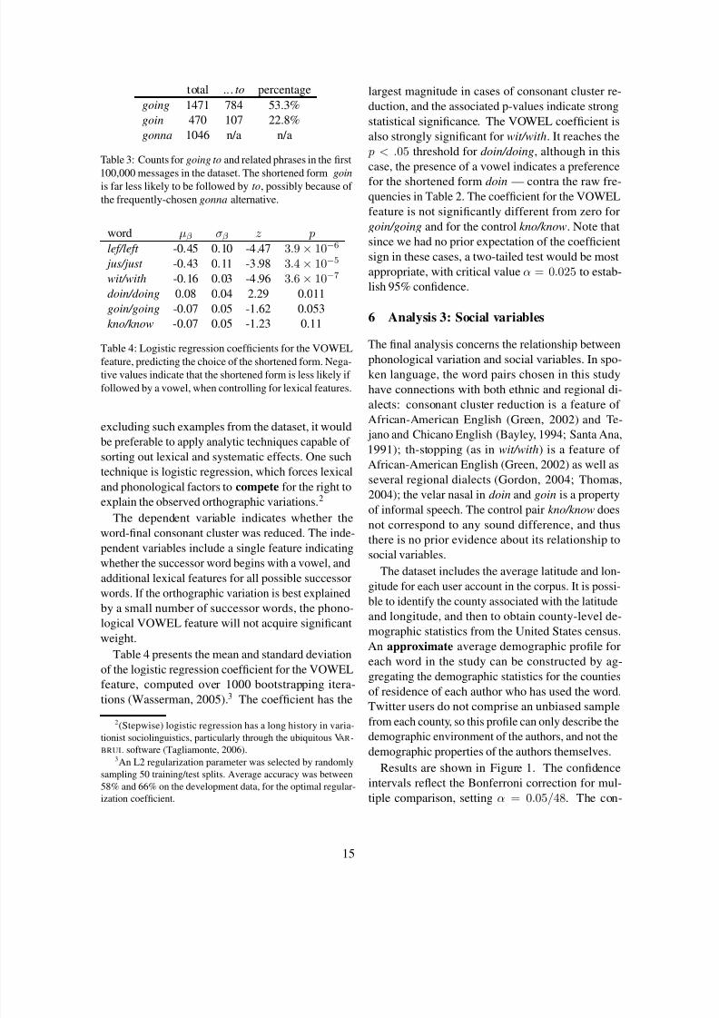
Results are shown in Figure 1. The confidence
intervals reflect the Bonferroni correction for mul-
tiple comparison, setting α = 0.05/48. The con-
15

8/13/2019 Workshop on Language Analysis in Social Media
http://slidepdf.com/reader/full/workshop-on-language-analysis-in-social-media 26/101
l e f l e f t j u s j u s t w i t w i t h g o i n g o i n g d o i n d o i n g k n o k n o w
1 6
1 8
2 0
2 2
2 4
2 6
2 8
3 0
%
b
l
a
c
k
l e f l e f t j u s j u s t w i t w i t h g o i n g o i n g d o i n d o i n g k n o k n o w
6 0
6 2
6 4
6 6
6 8
7 0
7 2
7 4
%
w
h
i
t
e
l e f l e f t j u s j u s t w i t w i t h g o i n g o i n g d o i n d o i n g k n o k n o w
1 4
1 6
1 8
2 0
2 2
2 4
%
h
i
s
p
a
n
i
c
l e f l e f t j u s j u s t w i t w i t h g o i n g o i n g d o i n d o i n g k n o k n o w
2 0 0 0
4 0 0 0
6 0 0 0
8 0 0 0
1 0 0 0 0
1 2 0 0 0
1 4 0 0 0
1 6 0 0 0
p
o
p
.
d
e
n
s
i
t
y
Figure 1: Average demographics of the counties in which users of each term live, with 95% confidence intervals
16

8/13/2019 Workshop on Language Analysis in Social Media
http://slidepdf.com/reader/full/workshop-on-language-analysis-in-social-media 27/101
sonant cluster reduction examples are indeed pre-
ferred by authors from densely-populated (urban)
counties with more African Americans, although
these counties tend to prefer all of the non-standard
variants, including the control pair kno/know. Con-
versely, the non-standard variants have aggregate
demographic profiles that include fewer EuropeanAmericans. None of the differences regarding the
percentage of Hispanics/Latinos are statistically sig-
nificant. Overall, these results show an associa-
tion between non-standard orthography and densely-
populated counties with high proportions of African
Americans, but we find no special affinity for conso-
nant cluster reduction.
7 Related work
Previous studies of the impact of dialect on writ-ing have found relatively little evidence of purely
phonological variation in written language. White-
man (1982) gathered an oral/written dataset of inter-
view transcripts and classroom compositions. In the
written data, there are many examples of final con-
sonant deletion: verbal -s (he go- to the pool), plural
-s (in their hand-), possessive -s (it is Sally- radio),
and past tense -ed . However, each of these deletions
is morphosyntactic rather than purely phonological.
They are seen by Whiteman as an omission of the
inflectional suffix, rather than as a transcription of
phonological variation, which she finds to be very
rare in cases where morphosyntactic factors are not in
play. She writes, “nonstandard phonological features
rarely occur in writing, even when these features are
extremely frequent in the oral dialect of the writer.”
Similar evidence is presented by Thompson et al.
(2004), who compare the spoken and written lan-
guage of 50 third-grade students who were identi-
fied as speakers of African American English (AAE).
While each of these students produced a substantial
amount of AAE in spoken language, they produced
only one third as many AAE features in the writtensample. Thompson et al. find almost no instances
of purely phonological features in writing, including
consonant cluster reduction — except in combina-
tion with morphosyntactic features, such as zero past
tense (e.g. mother kiss(ed) them all goodbye). They
propose the following explanation:
African American students have models
for spoken AAE; however, children do not
have models for written AAE... students
likely have minimal opportunities to ex-
perience AAE in print (emphasis in the
original).
This was written in 2004; in the intervening years,
social media and text messages now provide many
examples of written AAE. Unlike classroom settings,
social media is informal and outside the scope of
school control. Whether the increasing prevalence of
written AAE will ultimately lead to widely-accepted
writing systems for this and other dialects is an in-
triguing open question.
8 Conclusions and future work
The experiments in this paper demonstrate that
phonology impacts social media orthography at the
word level and beyond. I have discussed examples of
three such phenomena: consonant cluster reduction,
th-stopping, and the replacement of the velar nasal
with the coronal (“g-dropping”). Both consonant
cluster reduction and th-stopping are significantly in-
fluenced by the phonological context: their frequency
depends on whether the subsequent segment begins
with a vowel. This indicates that when social media
authors transcribe spoken language variation, they
are not simply replacing standard spellings of indi-
vidual words. The more difficult question — how
phonological context enters into writing — must be
left for future work.
There are several other avenues along which to con-
tinue this research. The sociolinguistic literature de-
scribes a number of other systematic factors that im-
pact consonant cluster reduction (Guy, 1991; Taglia-
monte and Temple, 2005), and a complete model that
included all such factors might shed additional light
on this phenomenon. In such work it is typical to dis-
tinguish between different types of consonants; for
example, Tagliamonte and Temple (2005) distinguish
obstruents, glides, pauses, and the liquids /r/ and /l/.In addition, while this paper has equated consonant
letters with consonant sounds, a more careful analy-
sis might attempt to induce (or annotate) the pronun-
ciation of the relevant words. The speech synthesis
literature offers numerous such methods (Bisani and
Ney, 2008), though social media text may pose new
17
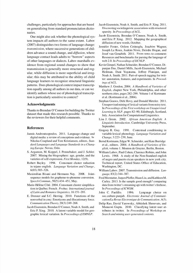
8/13/2019 Workshop on Language Analysis in Social Media
http://slidepdf.com/reader/full/workshop-on-language-analysis-in-social-media 28/101
challenges, particularly for approaches that are based
on generalizing from standard pronunciation dictio-
naries.
One might also ask whether the phonological sys-
tem impacts all authors to the same extent. Labov
(2007) distinguishes two forms of language change:
transmission, where successive generations of chil-
dren advance a sound change, and diffusion, where
language contact leads adults to “borrow” aspects
of other languages or dialects. Labov marshalls ev-
idence from regional sound changes to show that
transmission is generally more structural and reg-
ular, while diffusion is more superficial and irreg-
ular; this may be attributed to the ability of child
language learners to recognize structural linguistic
patterns. Does phonological context impact transcrip-
tion equally among all authors in our data, or can we
identify authors whose use of phonological transcrip-
tion is particularly sensitive to context?
Acknowledgments
Thanks to Brendan O’Connor for building the Twitterdataset that made this research possible. Thanks tothe reviewers for their helpful comments.
References
Jannis Androutsopoulos. 2011. Language change and
digital media: a review of conceptions and evidence. In
Nikolas Coupland and Tore Kristiansen, editors, Stan-
dard Languages and Language Standards in a Chang-
ing Europe. Novus, Oslo.
S. Argamon, M. Koppel, J. Pennebaker, and J. Schler.
2007. Mining the blogosphere: age, gender, and the
varieties of self-expression. First Monday, 12(9).
Robert Bayley. 1994. Consonant cluster reduction
in tejano english. Language Variation and Change,
6(03):303–326.
Maximilian Bisani and Hermann Ney. 2008. Joint-
sequence models for grapheme-to-phoneme conversion.
Speech Commun., 50(5):434–451, May.
Marie-Helene Cote. 2004. Consonant cluster simplifica-
tion in Quebec French. Probus: International journal
of Latin and Romance linguistics, 16:151–201.
E. Dresner and S.C. Herring. 2010. Functions of the
nonverbal in cmc: Emoticons and illocutionary force.
Communication Theory, 20(3):249–268.
Jacob Eisenstein, Brendan O’Connor, Noah A. Smith, and
Eric P. Xing. 2010. A latent variable model for geo-
graphic lexical variation. In Proceedings of EMNLP.
Jacob Eisenstein, Noah A. Smith, and Eric P. Xing. 2011.
Discovering sociolinguistic associations with structured
sparsity. In Proceedings of ACL.
Jacob Eisenstein, Brendan O’Connor, Noah A. Smith,
and Eric P. Xing. 2012. Mapping the geographical
diffusion of new words, October.
Jennifer Foster, Ozlem Cetinoglu, Joachim Wagner,Joseph Le Roux, Joakim Nivre, Deirdre Hogan, and
Josef van Genabith. 2011. From news to comment:
Resources and benchmarks for parsing the language of
web 2.0. In Proceedings of IJCNLP.
Kevin Gimpel, Nathan Schneider, Brendan O’Connor, Di-
panjan Das, Daniel Mills, Jacob Eisenstein, Michael
Heilman, Dani Yogatama, Jeffrey Flanigan, and
Noah A. Smith. 2011. Part-of-speech tagging for twit-
ter: annotation, features, and experiments. In Proceed-
ings of ACL.
Matthew J. Gordon, 2004. A Handbook of Varieties of
English, chapter New York, Philadelphia, and other
northern cities, pages 282–299. Volume 1 of Kortmann
et al. (Kortmann et al., 2004).
Stephan Gouws, Dirk Hovy, and Donald Metzler. 2011.
Unsupervised mining of lexical variants from noisy text.
In Proceedings of the First workshop on Unsupervised
Learning in NLP, pages 82–90, Edinburgh, Scotland,
July. Association for Computational Linguistics.
Lisa J. Green. 2002. African American English: A
Linguistic Introduction. Cambridge University Press,
September.
Gregory R. Guy. 1991. Contextual conditioning in
variable lexical phonology. Language Variation and
Change, 3:223–239, June.
Bernd Kortmann, Edgar W. Schneider, and Kate Burridge
et al., editors. 2004. A Handbook of Varieties of En-
glish, volume 1. Mouton de Gruyter, Berlin, Boston.
William Labov, Paul Cohen, Clarence Robins, and John
Lewis. 1968. A study of the Non-Standard english
of negro and puerto rican speakers in new york city.
Technical report, United States Office of Education,
Washington, DC.
William Labov. 2007. Transmission and diffusion. Lan-
guage, 83(2):344–387.
Fred Morstatter, Jurgen Pfeffer, Huan Liu, and Kathleen M.
Carley. 2013. Is the sample good enough? comparing
data from twitter’s streaming api with twitter’s firehose.
In Proceedings of ICWSM .
John C. Paolillo. 1996. Language choice on
soc.culture.punjab. Electronic Journal of Communi-
cation/La Revue Electronique de Communication, 6(3).
Delip Rao, David Yarowsky, Abhishek Shreevats, and
Manaswi Gupta. 2010. Classifying latent user at-
tributes in twitter. In Proceedings of Workshop on
Search and mining user-generated contents.
18

8/13/2019 Workshop on Language Analysis in Social Media
http://slidepdf.com/reader/full/workshop-on-language-analysis-in-social-media 29/101
Alan Ritter, Sam Clark, Mausam, and Oren Etzioni. 2011.
Named entity recognition in tweets: an experimental
study. In Proceedings of EMNLP.
Otto Santa Ana. 1991. Phonetic simplification processes
in the English of the barrio: A cross-generational soci-
olinguistic study of the Chicanos of Los Angeles. Ph.D.
thesis, University of Pennsylvania.
Aaron Smith and Joanna Brewer. 2012. Twitter use 2012.
Technical report, Pew Research Center, May.
Sali Tagliamonte and Rosalind Temple. 2005. New per-
spectives on an ol’ variable: (t,d) in british english.
Language Variation and Change, 17:281–302, Septem-
ber.
Sali A. Tagliamonte. 2006. Analysing Sociolinguistic
Variation. Cambridge University Press.
Erik R Thomas, 2004. A Handbook of Varieties of English,
chapter Rural Southern white accents, pages 87–114.
Volume 1 of Kortmann et al. (Kortmann et al., 2004).
Connie A. Thompson, Holly K. Craig, and Julie A. Wash-
ington. 2004. Variable production of african american
english across oracy and literacy contexts. Language,
speech, and hearing services in schools, 35(3):269–282,
July.
Jeffrey S. Vitter. 1985. Random sampling with a reservoir.
ACM Trans. Math. Softw., 11(1):37–57, March.
Larry Wasserman. 2005. All of Nonparametric Statistics
(Springer Texts in Statistics). Springer, October.
Marcia F. Whiteman. 1982. Dialect influence in writing.
In Marcia Farr Whiteman and Carl, editors, Writing:
The Nature, Development, and Teaching of Written
Communication, volume 1: Variation in writing. Rout-
ledge, October.
Benjamin Wing and Jason Baldridge. 2011. Simple su-
pervised document geolocation with geodesic grids. InProceedings of ACL.
19

8/13/2019 Workshop on Language Analysis in Social Media
http://slidepdf.com/reader/full/workshop-on-language-analysis-in-social-media 30/101
Proceedings of the Workshop on Language in Social Media (LASM 2013), pages 20–29,Atlanta, Georgia, June 13 2013. c2013 Association for Computational Linguistics
A Preliminary Study of Tweet Summarization using Information Extraction
Wei Xu, Ralph Grishman, Adam Meyers
Computer Science Department
New York UniversityNew York, NY 10003, USA
{xuwei,grishman,meyers}@cs.nyu.edu
Alan Ritter
Computer Science and Engineering
University of WashingtonSeattle, WA 98125, USA
Abstract
Although the ideal length of summaries dif-
fers greatly from topic to topic on Twitter, pre-
vious work has only generated summaries of a pre-fixed length. In this paper, we propose
an event-graph based method using informa-
tion extraction techniques that is able to cre-
ate summaries of variable length for different
topics. In particular, we extend the Pagerank-
like ranking algorithm from previous work to
partition event graphs and thereby detect fine-
grained aspects of the event to be summarized.
Our preliminary results show that summaries
created by our method are more concise and
news-worthy than SumBasic according to hu-
man judges. We also provide a brief survey of
datasets and evaluation design used in previ-ous work to highlight the need of developing a
standard evaluation for automatic tweet sum-
marization task.
1 Introduction
Tweets contain a wide variety of useful information
from many perspectives about important events tak-
ing place in the world. The huge number of mes-
sages, many containing irrelevant and redundant in-
formation, quickly leads to a situation of informa-tion overload. This motivates the need for automatic
summarization systems which can select a few mes-
sages for presentation to a user which cover the most
important information relating to the event without
redundancy and filter out irrelevant and personal in-
formation that is not of interest beyond the user’s
immediate social network.
Although there is much recent work focusing on
the task of multi-tweet summarization (Becker et al.,
2011; Inouye and Kalita, 2011; Zubiaga et al., 2012;
Liu et al., 2011a; Takamura et al., 2011; Harabagiu
and Hickl, 2011; Wei et al., 2012), most previouswork relies only on surface lexical clues, redun-
dancy and social network specific signals (e.g. user
relationship), and little work has considered taking
limited advantage of information extraction tech-
niques (Harabagiu and Hickl, 2011) in generative
models. Because of the noise and redundancy in
social media posts, the performance of off-the-shelf
news-trained natural language process systems is de-
graded while simple term frequency is proven pow-
erful for summarizing tweets (Inouye and Kalita,
2011). A natural and interesting research questionis whether it is beneficial to extract named entities
and events in the tweets as has been shown for clas-
sic multi-document summarization (Li et al., 2006).
Recent progress on building NLP tools for Twitter
(Ritter et al., 2011; Gimpel et al., 2011; Liu et al.,
2011b; Ritter et al., 2012; Liu et al., 2012) makes
it possible to investigate an approach to summariz-
ing Twitter events which is based on Information Ex-
traction techniques.
We investigate a graph-based approach which
leverages named entities, event phrases and theirconnections across tweets. A similar idea has been
studied by Li et al. (2006) to rank the salience
of event concepts in summarizing news articles.
However, the extreme redundancy and simplicity of
tweets allows us to explicitly split the event graph
into subcomponents that cover various aspects of the
initial event to be summarized to create comprehen-
20

8/13/2019 Workshop on Language Analysis in Social Media
http://slidepdf.com/reader/full/workshop-on-language-analysis-in-social-media 31/101
Work Dataset (size of each clus-
ter)
System Output Evaluation Metrics
Inouye and
Kalita (2011)
trending topics (approxi-
mately 1500 tweets)
4 tweets ROUGE and human (over-
all quality comparing to
human summary)
Sharifi et al.
(2010)
same as above 1 tweet same as above
Rosa et al.
(2011)
segmented hashtag top-
ics by LDA and k-means
clustering (average 410
tweets)
1, 5, 10 tweets Precision@k (relevance to
topic)
Harabagiu and
Hickl (2011)
real-word event topics (a
minimum of 2500 tweets)
top tweets until a limit of
250 words was reached
human (coverage and co-
herence)
Liu et al.
(2011a)
general topics and hash-
tag topics (average 1.7k
tweets)
same lengths as of the
human summary, vary
for each topic (about 2 or
3 tweets)
ROUGE and human (con-
tent coverage, grammat-
icality, non-redundancy,
referential clarity, focus)
Wei et al.(2012)
segmented hashtag top-ics according to burstiness
(average 10k tweets)
10 tweets ROUGE, Precison/Recall(good readability and rich
content)
Takamura et al.
(2011)
specific soccer games
(2.8k - 5.2k tweets)
same lengths as the hu-
man summary, vary for
each topic (26 - 41
tweets)
ROUGE (considering
only content words)
Chakrabarti and
Punera (2011)
specific football games
(1.8k tweets)
10 - 70 tweets Precision@k (relevance to
topic)
Table 1: Summary of datasets and evaluation metrics used in several previous work on tweet summarization
sive and non-redundant summaries. Our work is the
first to use a Pagerank-like algorithm for graph parti-
tioning and ranking in the context of summarization,
and the first to generate tweet summaries of variable
length which is particularly important for tweet sum-
marization. Unlike news articles, the amount of in-
formation in a set of topically clustered tweets varies
greatly, from very repetitive to very discrete. For ex-
ample, the tweets about one album release can be
more or less paraphrases, while those about another
album by a popular singer may involve rumors and
release events etc. In the human study conducted by
Inouye and Kalita (2011), annotators strongly prefer
different numbers of tweets in a summary for dif-
ferent topics. However, most of the previous work
produced summaries of a pre-fixed length and has
no evaluation on conciseness. Liu et al. (2011a)
and Takamura et al. (2011) also noticed the ideal
length of summaries can be very different from topic
to topic, and had to use the length of human refer-
ence summaries to decide the length of system out-
puts, information which is not available in practice.
In contrast, we developed a system that is capable
of detecting fine-grained sub-events and generating
summaries with the proper number of representative
tweets accordingly for different topics.
Our experimental results show that with informa-
tion extraction it is possible to create more mean-
ingful and concise summaries. Tweets that containreal-world events are usually more informative and
readable. Event-based summarization is especially
beneficial in this situation due to the fact that tweets
are short and self-contained with simple discourse
structure. The boundary of 140 characters makes it
efficient to extract semi-structured events with shal-
low natural language processing techniques and re-
21

8/13/2019 Workshop on Language Analysis in Social Media
http://slidepdf.com/reader/full/workshop-on-language-analysis-in-social-media 32/101
Tweets (Date Created) Named Entity Event Phrases Date Mentioned
Nooooo.. Season premiere of Doctor Who is on
Sept 1 world wide and we’ll be at World Con
(8/22/2012)
doctor who,
world con
season, is on,
premiere
sept 1
(9/1/2012)
guess what I DON’T get to do tomorrow!
WATCH DOCTOR WHO (8/31/2012)
doctor who watch tomorrow
(9/1/2012)
As I missed it on Saturday, I’m now catching upon Doctor Who (9/4/2012)
doctor who missed,catching up
saturday(9/1/2012)
Rumour: Nokia could announce two WP8 de-
vices on September 5 http://t.co/yZUwDFLV (via
@mobigyaan)
nokia, wp8 announce september 5
(9/5/2012)
Verizon and Motorola won’t let Nokia have all
the fun ; scheduling September 5th in New York
http://t.co/qbBlYnSl (8/19/2012)
nokia, verizon,
motorola,
new york
scheduling september 5th
(9/5/2012)
Don’t know if it’s excitement or rooting for the
underdog, but I am genuinely excited for Nokia
come Sept 5: http://t.co/UhV5SUMP (8/7/2012)
nokia rooting,
excited
sept 5
(9/5/2012)
Table 2: Event-related information extracted from tweets
duces the complexity of the relationship (or no re-
lationship) between events according to their co-
occurrence, resulting in differences in constructing
event graphs from previous work in news domain
(Li et al., 2006).
2 Issues in Current Research on Tweet
Summarization
The most serious problem in tweet summarizationis that there is no standard dataset, and conse-
quently no standard evaluation methodology. Al-
though there are more than a dozen recent works on
social media summarization, astonishingly, almost
each research group used a different dataset and a
different experiment setup. This is largely attributed
to the difficulty of defining the right granularity of a
topic in Twitter. In Table 1, we summarize the exper-
iment designs of several selective works. Regardless
of the differences, researchers generally agreed on :
• clustering tweets topically and temporally
• generating either a very short summary for a
focused topic or a long summary for large-size
clusters
• difficulty and necessity to generate summaries
of variable length for different topics
Although the need of variable-length summaries
have been raised in previous work, none has pro-
vide a good solution (Liu et al., 2011a; Takamura
et al., 2011; Inouye and Kalita, 2011). In this pa-
per, our focus is study the feasibility of generating
concise summaries of variable length and improv-
ing meaningfulness by using information extraction
techniques. We hope this study can provide new in-
sights on the task and help in developing a standard
evaluation in the future.
3 Approach
We first extract event information including named
entities and event phrases from tweets and construct
event graphs that represent the relationship between
them. We then rank and partition the events using
PageRank-like algorithms, and create summaries of
variable length for different topics.
3.1 Event Extraction from Tweets
As a first step towards summarizing popular events
discussed on Twitter, we need a way to identify
events from Tweets. We utilize several natural lan-
guage processing tools that specially developed for
noisy text to extract text phrases that bear essential
event information, including named entities (Ritter
et al., 2011), event-referring phrases (Ritter et al.,
22

8/13/2019 Workshop on Language Analysis in Social Media
http://slidepdf.com/reader/full/workshop-on-language-analysis-in-social-media 33/101

8/13/2019 Workshop on Language Analysis in Social Media
http://slidepdf.com/reader/full/workshop-on-language-analysis-in-social-media 34/101
Starting from arbitrary values assigned to each
node in the graph, the computation iterates until con-
vergence. Note that the final salience score of each
node is not affected by the choice of the initial val-
ues assigned to each node in the graph, but rather the
weights of edges.
In previous work computed scores are then useddirectly to select text fractions for summaries (Li et
al., 2006). However, the redundancy and simplic-
ity of tweets allow further exploration into sub-event
detection by graph partitioning. The intuition is that
the correlations between named entities and event
phrases within same sub-events are much stronger
than between sub-events. This phenomena is more
obvious and clear in tweet than in news articles,
where events are more diverse and complicated re-
lated to each other given lengthy context.
As theoretically studied in local partitioning prob-
lem (Andersen et al., 2006), a good partition of the
graph can be obtained by separating high ranked ver-
tices from low ranked vertices, if the nodes in the
graph have ranks that are distinguishable. Utilizing
a similar idea, we show that a simple greedy algo-
rithm is efficient to find important sub-events and
generate useful summaries in our tasks. As shown
in Figure 2 and 3, the high ranked nodes (whose
scores are greater than 1, the average score of all
nodes in the graph) in tweet event graphs show the
divisions within a topic. We search for strongly con-
nected sub-graphs, as gauged by parameter α, fromthe highest ranked node to lower ranked ones.The
proportion of tweets in a set that are related to a
sub-event is then estimated according to the ratio be-
tween the sum of node scores in the sub-graph ver-
sus the entire graph. We select one tweet for each
sub-event that best covers the related nodes with the
highest sum of node scores normalized by length as
summaries. By adding a cutoff (parameter β ) on
proportion of sub-event required to be included into
summaries, we can produce summaries with the ap-
propriate length according to the diversity of infor-mation in a set of tweets.
In Figure 2, 3 and 4, the named entity which is
also the topic of tweet cluster is omitted since it is
connected with every node in the event graph. The
size of node represents the salience score, while the
shorter, straighter and more vertical the edge is, the
higher its weight. The nodes with rectangle shapes
Algorithm 1 Find important sub-events
Require: Ranked event graph G = (V, E ), the
named entity V 0 which is the topic of event
cluster, parameters α and β that can be set
towards user preference over development data
1: Initialize the pool of high ranked nodesV ← {V i|∀V i ∈ V, S (V i) > 1} − V 0 and the
total weight W ←P
V i∈V S (V i)
2: while V 6= ∅ do
3: Pop the highest ranked node V m from V 4: Put V m to a temporary sub-event e ← {V m}5: for all V n in V do
6: if wmn/w0m > α and w0n/w0m > α
then
7: e ← e ∪ {V n}8: end if
9: end for10: W e ←
PV i∈e
S (V i)11: if W e/W > β then
12: Successfully find a sub-event e13: Remove all nodes in e from V 14: end if
15: end while
are named entities, while round shaped ones are
event phrases. Note that in most cases, sub-events
correspond to connected components in the event
graph of high ranked nodes as in Figure 2 and 3.
However, our simple greedy algorithm also allows
multiple sub-events for a single connected compo-
nent that can not be covered by one tweet in the
summary. For example, in Figure 4, two sub-events
e1 = {sell, delete, start, payment} and e2 ={f acebook, share user data, privacy policy, debut}are chosen to accommodate the complex event.
4 Experiments
4.1 Data
We gathered tweets over a 4-month period spanning
November 2012 to February 2013 using the Twitter
Streaming API. As described in more details in pre-
vious work on Twitter event extraction by Ritter et
al. (2012), we grouped together all tweets which
mention the same named entity (recognized using
24

8/13/2019 Workshop on Language Analysis in Social Media
http://slidepdf.com/reader/full/workshop-on-language-analysis-in-social-media 35/101
Figure 2: Event graph of ’Google - 1/16/2013’, an example of event cluster with multiple focuses
Figure 3: Event graph of ’Instagram - 1/16/2013’, an example of event cluster with a single but complex focus
25

8/13/2019 Workshop on Language Analysis in Social Media
http://slidepdf.com/reader/full/workshop-on-language-analysis-in-social-media 36/101
Figure 4: Event graph of ’West Ham - 1/16/2013’, an
example of event cluster with a single focus
a Twitter specific name entity tagger1) and a refer-
ence to the same unique calendar date (resolved us-
ing a temporal expression processor (Mani and Wil-
son, 2000)). Tweets published during the whole pe-
riod are aggregated together to find top events that
happen on each calendar day. We applied the G2
test for statistical significance (Dunning, 1993) to
rank the event clusters, considering the corpus fre-
quency of the named entity, the number of times the
date has been mentioned, and the number of tweets
which mention both together. We randomly picked
the events of one day for human evaluation, that is
the day of January 16, 2013 with 38 events and an
average of 465 tweets per event cluster.
For each cluster, our systems produce two ver-
sions of summaries, one with a fixed number (set
to 3) of tweets and another one with a flexible num-
ber (vary from 1 to 4) of tweets. Both α and β are
set to 0.1 in our implementation. All parameters are
set experimentally over a small development dataset
consisting of 10 events in Twitter data of September
2012.
1https://github.com/aritter/twitter_nlp
4.2 Baseline
SumBasic (Vanderwende et al., 2007) is a simple
and effective summarization approach based on term
frequency, which we use as our baseline. It uses
word probabilities with an update function to avoid
redundancy to select sentences or posts in a social
media setting. It is shown to outperform three other
well-known multi-document summarization meth-
ods, namely LexRank (Erkan and Radev, 2004),
TextRank (Mihalcea and Tarau, 2004) and MEAD
(Radev et al., 2004) on tweets in (Inouye and Kalita,
2011), possibly because that the relationship be-
tween tweets is much simpler than between sen-
tences in news articles and can be well captured by
simple frequency methods. The improvement over
the LexRank model on tweets is gained by consid-
ering the number of retweets and influential users is
another side-proof (Wei et al., 2012) of the effective-ness of frequency.
EventRank!Flexible EventRank!Fixed SumBasi c
Annotator 1
0
1
2
3
4
5
compactness
completenessoverall
EventRank!Flexible EventRank!Fixed SumBasi c
Annotator 2
0
1
2
3
4
5
compactnesscompleteness
overall
Figure 5: human judgments evaluating tweet summariza-
tion systems
26

8/13/2019 Workshop on Language Analysis in Social Media
http://slidepdf.com/reader/full/workshop-on-language-analysis-in-social-media 37/101
Event System Summary
- Google ’s home page is a Zamboni game in celebration of Frank Zam-
boni ’s birthday January 16 #GameOn
EventRank
(Flexible)
- Today social , Tomorrow Google ! Facebook Has Publicly Redefined
Itself As A Search Company http://t.co/dAevB2V0 via @sai
1/16/2013
- Orange says has it has forced Google to pay for traffic . The Head of
the Orange said on Wednesday it had ... http://t.co/dOqAHhWi- Tomorrow’s Google doodle is going to be a Zamboni! I may have to
take a vacation day.
SumBasic - the game on google today reminds me of hockey #tooexcited #saturday
- The fact that I was soooo involved in that google doodle game says
something about this Wednesday #TGIW You should try it!
EventRank
(Flexible)
- So Instagram can sell your pictures to advertisers without u knowing
starting January 16th I’m bout to delete my instagram !
- Instagram debuts new privacy policy , set to share user data with Face-
book beginning January 16
1/16/2013
- Instagram will have the rights to sell your photos to Advertisers as of
jan 16SumBasic - Over for Instagram on January 16th
- Instagram says it now has the right to sell your photos unless you delete
your account by January 16th http://t.co/tsjic6yA
EventRank
(Flexible)
- RT @Bassa_Mufc : Wayne Rooney and Nani will feature in the FA Cup
replay with West Ham on Wednesday - Sir Alex Ferguson
West Ham
1/16/2013
- Wayne Rooney could be back to face West Ham in next Wednesday’s
FA Cup replay at Old Trafford. #BPL
SumBasic - Tomorrow night come on West Ham lol
- Nani’s fit abd WILL play tomorrow against West Ham! Sir Alex con-
firmed :)
Table 3: Event-related information extracted from tweets
4.3 Preliminary Results
We performed a human evaluation in which two an-
notators were asked to rate the system on a five-
point scale (1=very poor, 5=very good) for com-
pleteness and compactness. Completeness refers to
how well the summary cover the important content
in the tweets. Compactness refers to how much
meaningful and non-redundant information is in the
summary. Because the tweets were collected ac-cording to information extraction results and ranked
by salience, the readability of summaries generated
by different systems are generally very good. The
top 38 events of January 16, 2013 are used as test
set. The aggregate results of the human evaluation
are displayed in Figure 5. Agreement between an-
notators measured using Pearson’s Correlation Co-
efficient is 0.59, 0.62, 0.62 respectively for compact-
ness, completeness and overall judgements.
Results suggest that the models described in this
paper produce more satisfactory results as the base-
line approaches. The improvement of EventRank-
Flexible over SumBasic is significant (two-tailed
p < 0.05) for all three metrics according to stu-
dent’s t test. Example summaries of the events in
Figure 2, 3 and 4 are presented respectively in Table3. The advantages of our method are the follow-
ing: 1) it finds important facts of real-world events
2) it prefers tweets with good readability 3) it in-
cludes the right amount of information with diversity
and without redundancy. For example, our system
picked only one tweet about ’West Ham -1/16/2013’
that convey the same message as the three tweets to-
27
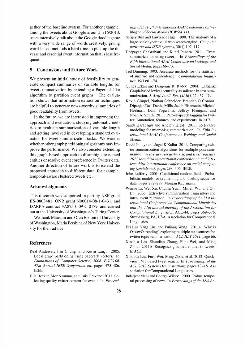
8/13/2019 Workshop on Language Analysis in Social Media
http://slidepdf.com/reader/full/workshop-on-language-analysis-in-social-media 38/101

8/13/2019 Workshop on Language Analysis in Social Media
http://slidepdf.com/reader/full/workshop-on-language-analysis-in-social-media 39/101
nual Meeting on Association for Computational Lin-
guistics, ACL ’00, pages 69–76, Stroudsburg, PA,
USA. Association for Computational Linguistics.
Rada Mihalcea and Paul Tarau. 2004. Textrank: Bring-
ing order into texts. In Proceedings of EMNLP, vol-
ume 4, pages 404–411. Barcelona, Spain.
Dragomir Radev, Timothy Allison, Sasha Blair-
Goldensohn, John Blitzer, Arda Celebi, StankoDimitrov, Elliott Drabek, Ali Hakim, Wai Lam, Danyu
Liu, et al. 2004. Mead-a platform for multidocument
multilingual text summarization. In Proceedings of
LREC , volume 2004.
Alan Ritter, Sam Clark, Mausam, and Oren Etzioni.
2011. Named entity recognition in tweets: An experi-
mental study.
Alan Ritter, Mausam, Oren Etzioni, and Sam Clark.
2012. Open domain event extraction from twitter. In
KDD, pages 1104–1112. ACM.
Kevin Dela Rosa, Rushin Shah, Bo Lin, Anatole Gersh-
man, and Robert Frederking. 2011. Topical clustering
of tweets. Proceedings of the ACM SIGIR: SWSM .
Beaux Sharifi, Mark-Anthony Hutton, and Jugal K
Kalita. 2010. Experiments in microblog summariza-
tion. In Proc. of IEEE Second International Confer-
ence on Social Computing.
Hiroya Takamura, Hikaru Yokono, and Manabu Oku-
mura. 2011. Summarizing a document stream. Ad-
vances in Information Retrieval, pages 177–188.
Lucy Vanderwende, Hisami Suzuki, Chris Brockett, and
Ani Nenkova. 2007. Beyond sumbasic: Task-focused
summarization with sentence simplification and lex-
ical expansion. Information Processing & Manage-
ment , 43(6):1606–1618.Furu Wei, Ming Zhou, and Heung-Yeung Shum. 2012.
Twitter topic summarization by ranking tweets using
social influence and content quality. In COLING.
Arkaitz Zubiaga, Damiano Spina, Enrique Amigó, and
Julio Gonzalo. 2012. Towards real-time summariza-
tion of scheduled events from twitter streams. In Pro-
ceedings of the 23rd ACM conference on Hypertext
and social media, pages 319–320. ACM.
29

8/13/2019 Workshop on Language Analysis in Social Media
http://slidepdf.com/reader/full/workshop-on-language-analysis-in-social-media 40/101
Proceedings of the Workshop on Language in Social Media (LASM 2013), pages 30–40,Atlanta, Georgia, June 13 2013. c2013 Association for Computational Linguistics
Really? Well. Apparently Bootstrapping Improves the Performance of
Sarcasm and Nastiness Classifiers for Online Dialogue
Stephanie LukinNatural Language and Dialogue Systems
University of California, Santa Cruz1156 High Street, Santa Cruz, CA [email protected]
Marilyn WalkerNatural Language and Dialogue Systems
University of California, Santa Cruz1156 High Street, Santa Cruz, CA [email protected]
Abstract
More and more of the information on the webis dialogic, from Facebook newsfeeds, to fo-rum conversations, to comment threads onnews articles. In contrast to traditional, mono-logic Natural Language Processing resources
such as news, highly social dialogue is fre-quent in social media, making it a challengingcontext for NLP. This paper tests a bootstrap-ping method, originally proposed in a mono-logic domain, to train classifiers to identifytwo different types of subjective language indialogue: sarcasm and nastiness. We exploretwo methods of developing linguistic indica-tors to be used in a first level classifier aimedat maximizing precision at the expense of re-call. The best performing classifier for the firstphase achieves 54% precision and 38% recallfor sarcastic utterances. We then use generalsyntactic patterns from previous work to cre-
ate more general sarcasm indicators, improv-ing precision to 62% and recall to 52%. Tofurther test the generality of the method, wethen apply it to bootstrapping a classifier fornastiness dialogic acts. Our first phase, usingcrowdsourced nasty indicators, achieves 58%precision and 49% recall, which increases to75% precision and 62% recall when we boot-strap over the first level with generalized syn-tactic patterns.
1 Introduction
More and more of the information on the web isdialogic, from Facebook newsfeeds, to forum con-
versations, to comment threads on news articles. In
contrast to traditional, monologic Natural Language
Processing resources such as news, highly social di-
alogue is very frequent in social media, as illustrated
in the snippets in Fig. 1 from the publicly avail-
able Internet Argument Corpus (IAC) (Walker et al.,
Quote Q, Response R Sarc Nasty
Q1: I jsut voted. sorry if some people actu-ally have, you know, LIVES and don’t sit aroundall day on debate forums to cater to some athe-ists posts that he thiks they should drop every-thing for. emoticon-rolleyes emoticon-rolleyesemoticon-rolleyes As to the rest of yourpost, well,from your attitude I can tell you are not Christianin the least. Therefore I am content in knowing
where people that spew garbage like this will endup in the End.R1: No, let me guess . . . er . . . McDonalds. No,Disneyland. Am I getting closer?
1 -3.6
Q2: The key issue is that once children are bornthey are not physically dependent on a particularindividual.R2 Really? Well, when I have a kid, I’ll be sure to
just leave it in the woods, since it can apparentlycare for itself.
1 -1
Q3: okay, well i think that you are just findingreasons to go against Him. I think that you hadsome bad experiances when you were younger ora while ago that made you turn on God. You arelooking for reasons, not very good ones i mightadd, to convince people.....either way, God lovesyou. :)
R3: Here come the Christians, thinking they canknow everything by guessing, and commiting thegenetic fallacy left and right.
0.8 -3.4
Figure 1: Sample Quote/Response Pairs from4forums.com with Mechanical Turk annotationsfor Sarcasm and Nasty/Nice. Highly negative valuesof Nasty/Nice indicate strong nastiness and sarcasm isindicated by values near 1.
2012). Utterances are frequently sarcastic, e.g., Re-
ally? Well, when I have a kid, I’ll be sure to just
leave it in the woods, since it can apparently care
for itself (R2 in Fig. 1 as well as Q1 and R1), and are
often nasty, e.g. Here come the Christians, thinkingthey can know everything by guessing, and commit-
ing the genetic fallacy left and right (R3 in Fig. 1).
Note also the frequent use of dialogue specific dis-
course cues, e.g. the use of No in R1, Really? Well
in R2, and okay, well in Q3 in Fig. 1 (Fox Tree
and Schrock, 1999; Bryant and Fox Tree, 2002; Fox
Tree, 2010).
30

8/13/2019 Workshop on Language Analysis in Social Media
http://slidepdf.com/reader/full/workshop-on-language-analysis-in-social-media 41/101
The IAC comes with annotations of different
types of social language categories including sarcas-
tic vs not sarcastic, nasty vs nice, rational vs emo-
tional and respectful vs insulting. Using a conser-
vative threshold of agreement amongst the annota-
tors, an analysis of 10,003 Quote/Response pairs
(Q/R pairs) from the 4forums portion of IAC sug-
gests that social subjective language is fairly fre-quent: about 12% of posts are sarcastic, 23% are
emotional, and 12% are insulting or nasty. We select
sarcastic and nasty dialogic turns to test our method
on more than one type of subjective language and
explore issues of generalization; we do not claim any
relationship between these types of social language
in this work.
Despite their frequency, expanding this corpus of
sarcastic or nasty utterances at scale is expensive:
human annotation of 100% of the corpus would be
needed to identify 12% more examples of sarcasm
or nastiness. An explanation of how utterances areannotated in IAC is detailed in Sec. 2.
Our aim in this paper is to explore whether it is
possible to extend a method for bootstrapping a clas-
sifier for monologic, subjective sentences proposed
by Riloff & Wiebe, henceforth R&W (Riloff and
Wiebe, 2003; Thelen and Riloff, 2002), to automat-
ically find sarcastic and nasty utterances in unanno-
tated online dialogues. Sec. 3 provides an overview
of R&W’s bootstrapping method. To apply boot-
strapping, we:
1. Explore two different methods for identifying
cue words and phrases in two types of subjec-
tive language in dialogues: sarcasm and nasty
(Sec. 4);
2. Use the learned indicators to train a sarcastic
(nasty) dialogue act classifier that maximizes
precision at the expense of recall (Sec. 5);
3. Use the classified utterances to learn general
syntactic extraction patterns from the sarcastic
(nasty) utterances (Sec. 6);
4. Bootstrap this process on unannotated text to
learn new extraction patterns to use for classifi-
cation.We show that the Extraction Pattern Learner im-
proves the precision of our sarcasm classifier by
17% and the recall by 24%, and improves the pre-
cision of the nastiness classifier by 14% and recall
by 13%. We discuss previous work in Sec. 2 and
compare to ours in Sec. 7 where we also summarize
our results and discuss future work.
2 Previous Work
IAC provides labels for sarcasm and nastiness that
were collected with Mechanical Turk on Q/R pairs
such as those in Fig. 1. Seven Turkers per Q/R pair
answered a binary annotation question for sarcasm
Is the respondent using sarcasm? (0,1) and a scalar
annotation question for nastiness Is the respondent
attempting to be nice or is their attitude fairly nasty?
(-5 nasty . . . 5 nice). We selected turns from IAC
Table 1 with sarcasm averages above 0.5, and nasty
averages below -1 and nice above 1. Fig. 1 included
example nastiness and sarcasm values.
Previous work on the automatic identification
of sarcasm has focused on Twitter using the
#sarcasm (Gonzalez-Ibanez et al., 2011) and
#irony (Reyes et al., 2012) tags and a combined
variety of tags and smileys (Davidov et al., 2010).
Another popular domain examines Amazon product
reviews looking for irony (Reyes and Rosso, 2011),
sarcasm (Tsur et al., 2010), and a corpus collec-
tion for sarcasm (Filatova, 2012). (Carvalho et al.,
2009) looks for irony in comments in online newpa-
pers which can have a thread-like structure. This
primary focus on monologic venues suggests that
sarcasm and irony can be detected with a relatively
high precision but have a different structure from di-
alogues (Fox Tree and Schrock, 1999; Bryant and
Fox Tree, 2002; Fox Tree, 2010), posing the ques-
tion, can we generalize from monologic to dialogic
structures? Each of these works use methods in-
cluding LIWC unigrams, affect, polarity, punctua-
tion and more, and achieve on average a precision of
75% or accuracy of between 45% and 85%.
Automatically identifying offensive utterances is
also of interest. Previous work includes identifying
flames in emails (Spertus, 1997) and other messag-
ing interfaces (Razavi et al., 2010), identifying in-
sults in Twitter (Xiang et al., 2012), as well as com-
ments from new sites (Sood et al., 2011). These
approaches achieve an accuracy between 64% and
83% using a variety of approaches. The accuracies
for nasty utterances has a much smaller spread and
higher average than sarcasm accuracies. This sug-
gests that nasty language may be easier to identify
than sarcastic language.
3 Method Overview
Our method for bootstrapping a classifier for sarcas-
tic (nasty) dialogue acts uses R&W’s model adapted
to our data as illustrated for sarcasm in Fig. 2. The
31

8/13/2019 Workshop on Language Analysis in Social Media
http://slidepdf.com/reader/full/workshop-on-language-analysis-in-social-media 42/101

8/13/2019 Workshop on Language Analysis in Social Media
http://slidepdf.com/reader/full/workshop-on-language-analysis-in-social-media 43/101
describe how we use the “PE eval” development set
(Table 1) to estimate parameters for the Extraction
Pattern Learner, and then test the Pattern Based Sar-
castic (Nasty) Post classifier on the newly classified
utterances from the dataset labeled “HP dev test”
(Table 1). Our final open question was whether the
extraction patterns from R&W, which worked well
for news text, would work on social dialogue (O3below). Thus our experiments address the following
open questions as to whether R&W’s bootstrapping
method improves classifiers for sarcasm and nasti-
ness in online dialogues:
• (O1) Can we develop a “known sarcastic
(nasty) vocabulary”? The LH circle of Fig. 2
illustrates that we use two different methods to
identify Sarcasm Cues. Because we have ut-
terances labeled as sarcastic, we compare a sta-
tistical method that extracts important features
automatically from utterances, with a method
that has a human in the loop, asking annotators
to select phrases that are good indicators of sar-
casm (nastiness) (Sec. 5);
• (O2) If we can develop a reliable set of sarcasm
(nastiness) cues, is it then possible to develop
an HP classifier? Will our precision be high
enough? Is the fact that sarcasm is often con-
text dependent an issue? (Sec. 5);
• (O3) Will the extraction patterns used in
R&W’s work allow us to generalize sarcasm
cues from the HP Classifiers? Are R&W’s pat-
terns general enough to work well for dialogueand social language? (Sec. 6).
4 Sarcasm and Nastiness Cues
Because there is no prior “Known Sarcastic Vocabu-
lary” we pilot two different methods for discovering
lexical cues to sarcasm and nastiness, and experi-
ment with combinations of cues that could yield a
high precision classifier (Gianfortoni et al., 2011).
The first method uses χ2 to measure whether a word
or phrase is statistically indicative of sarcasm (nasti-
ness) in the development sets labeled “MT exp dev”
(Table 1). This method, a priori, seems reasonablebecause it is likely that if you have a large enough
set of utterances labeled as sarcastic, you could be
able to automatically learn a set of reliable cues for
sarcasm.
The second method introduces a step of human
annotation. We ask Turkers to identify sarcastic
(nasty) indicators in utterances (the open question
unigram
χ2 MT IA FREQ
right ah .95 2
oh relevant .85 2
we amazing .80 2
same haha .75 2
all yea .73 3
them thanks .68 6
mean oh .56 56
bigramχ2 MT IA FREQ
the same oh really .83 2
mean like oh yeah .79 2
trying to so sure .75 2
that you no way .72 3
oh yeah get real .70 2
I think oh no .66 4
we should you claim .65 2
trigramχ2 MT IA FREQ
you mean to I get it .97 3mean to tell I’m so sure .65 2
have to worry then of course .65 2
sounds like a are you saying .60 2
to deal with well if you .55 2
I know I go for it .52 2
you mean to oh, sorry .50 2
Table 2: Mechanical Turk (MT) and χ2 indicators forSarcasm
O1) from the development set “MT exp dev” (Ta-
ble 1). Turkers were presented with utterances pre-viously labeled sarcastic or nasty in IAC by 7 dif-
ferent Turkers, and were told “In a previous study,
these responses were identified as being sarcastic by
3 out of 4 Turkers. For each quote/response pair,
we will ask you to identify sarcastic or potentially
sarcastic phrases in the response”. The Turkers then
selected words or phrases from the response they be-
lieved could lead someone to believing the utterance
was sarcastic or nasty. These utterances were not
used again in further experiments. This crowdsourc-
ing method is similar to (Filatova, 2012), but where
their data is monologic, ours is dialogic.
4.1 Results from Indicator Cues
Sarcasm is known to be highly variable in form, and
to depend, in some cases, on context for its inter-
pretation (Sperber and Wilson, 1981; Gibbs, 2000;
Bryant and Fox Tree, 2002). We conducted an ini-
tial pilot on 100 of the 617 sarcastic utterances in
33

8/13/2019 Workshop on Language Analysis in Social Media
http://slidepdf.com/reader/full/workshop-on-language-analysis-in-social-media 44/101
unigram
χ2 MT IA FREQ
like idiot .90 3
them unfounded .85 2
too babbling .80 2
oh lie .72 11
mean selfish .70 2
just nonsense .69 9
make hurt .67 3
bigramχ2 MT IA FREQ
of the don’t expect .95 2
you mean get your .90 2
yes, you’re an .85 2
oh, what’s your .77 4
you are prove it .77 3
like a get real .75 2
I think what else .70 2
trigramχ2 MT IA FREQ
to tell me get your sick .75 2would deny a your ignorance is .70 2
like that? make up your .70 2
mean to tell do you really .70 2
sounds like a do you actually .65 2
you mean to doesn’t make it .63 3
to deal with what’s your point .60 2
Table 3: Mechanical Turk (MT) and χ2 indicators forNasty
Figure 3: Interannotator Agreement for sarcasm trigrams
the development set “MT exp dev” to see if this was
necessarily the case in our dialogues. (Snow et al.,
2008) measures the quality of Mechanical Turk an-
notations on common NLP tasks by comparing them
to a gold standard. Pearson’s correlation coefficient
shows that very few Mechanical Turk annotators
were required to beat the gold standard data, often
less than 5. Because our sarcasm task does not have
gold standard data, we ask 100 annotators to partic-
ipate in the pilot. Fig. 3 plots the average interan-
notator agreement (ITA) as a function of the number
of annotators, computed using Pearson correlation
counts, for 40 annotators and for trigrams which re-
quire more data to converge. In all cases (unigrams,
bigrams, trigrams) ITA plateaus at around 20 anno-tators and is about 90% with 10 annotators, showing
that the Mechanical Turk tasks are well formed and
there is high agreement. Thus we elicited only 10
annotations for the remainder of the sarcastic and all
the nasty utterances from the development set “MT
exp dev”.
We begin to form our “known sarcastic vocab-
ulary” from these indicators, (open question O1).
Each MT indicator has a FREQ (frequency): the
number of times each indicator appears in the train-
ing set; and an IA (interannotator agreement): how
many annotators agreed that each indicator was sar-castic or nasty. Table 2 shows the best unigrams,
bigrams, and trigrams from the χ2 test and from the
sarcasm Mechanical Turk experiment and Table 3
shows the results from the nasty experiment. We
compare the MT indicators to the χ2 indicators as
part of investigating open question O1.
As a pure statistical method, χ2 can pick out
things humans might not. For example, if it just hap-
pened that the word ‘we’ only occurs in sarcastic
utterances in the development set, then χ2 will se-
lect it as a strong sarcastic word (row 3 of Table 2).
However, no human would recognize this word ascorresponding to sarcasm. χ2 could easily be over-
trained if the “MT exp dev” development set is not
large enough to eliminate such general words from
consideration, “MT exp dev” only has 617 sarcastic
utterances and 510 nasty utterances (Table 1).
Words that the annotators select as indicators
(columns labeled MT in Table 2 and Table 3) are
much more easily identifiable although they do not
appear as often. For example, the IA of 0.95 for ‘ah’
in Table 2 means that of all the annotators who saw
‘ah’ in the utterance they annotated, 95% selected it
to be sarcastic. However the FREQ of 2 means that‘ah’ only appeared in 2 utterances in the “MT exp
dev” development set.
We test whether any of the methods for select-
ing indicators provide reliable cues that generalize
to a larger dataset in Sec. 5. The parameters that
we estimate on the development sets are exactly how
frequent (compared to a θ1) and how reliable (com-
34

8/13/2019 Workshop on Language Analysis in Social Media
http://slidepdf.com/reader/full/workshop-on-language-analysis-in-social-media 45/101
pared to a θ2) a cue has to be to be useful in R&W’s
bootstrapping method.
5 High-Precision Classifiers
R&W use their “known subjective vocabulary” to
train a High Precision classifier. R&W’s HP classi-
fier searches for exact surface matches of the sub- jective indicators and classifies utterances as sub-
jective if two subjective indicators are present. We
follow similar guidelines to train HP Sarcasm and
Nasty Classifiers. To test open question O1, we
use a development set called “HP train” (Table 1)
to test three methods for measuring the “goodness”
of an indicator that could serve as a high precision
cue: (1) interannotator agreement based on anno-
tators consensus from Mechanical Turk, on the as-
sumption that the number of annotators that select
a cue indicates its strength and reliability ( IA fea-
tures); (2) percent sarcastic (nasty) and frequencystatistics in the HP train dataset as R&W do ( percent
features); and (3) the χ2 percent sarcastic (nasty)
and frequency statistics (χ2 features).
The IA features use the MT indicators and the IA
and FREQ calculations introduced in Sec. 4 (see
Tables 2 and 3). First, we select indicators such
that θ1 <= FREQ where θ1 is a set of possible
thresholds. Then we introduce two new parameters
α and β to divide the indicators into three “good-
ness” groups that reflect interannotator agreement.
indicatorstrength = weak if 0 ≤ IA < α
medium if α ≤ IA < β strong if β ≤ IA < 1
For IA features, an utterance is classified as sar-
castic if it contains at least one strong or two medium
indicators. Other conditions were piloted. We first
hypothesized that weak cues might be a way of
classifying “not sarcastic” utterances. But HP train
showed that both sarcastic and not sarcastic utter-
ances contain weak indicators yielding no informa-
tion gain. The same is true for Nasty’s counter-
class Nice. Thus we specify that counter-class utter-
ances must have no strong indicators or at most onemedium indicator. In contrast, R&W’s counter-class
classifier looks for a maximum of one subjective in-
dicator.
The percent features also rely on the FREQ of
each MT indicator, subject to a θ1 threshold, as
well as the percentage of the time they occur in
a sarcastic utterance (%SARC) or nasty utterance
(%NASTY). We select indicators with various pa-
rameters for θ1 and θ2 ≤ %SARC. At least two in-
dicators must be present and above the thresholds to
be classified and we exhaust all combinations. Less
than two indicators are needed to be classified as the
counter-class, as in R&W.
Finally, the χ2 features use the same method as
percent features only using the χ2
indicators insteadof the MT indicators.
After determining which parameter settings per-
forms the best for each feature set, we ran the HP
classifiers, using each feature set and the best param-
eters, on the test set labeled “HP dev test”. The HP
Classifiers classify the utterances that it is confident
on, and leave others unlabeled.
5.1 Results from High Precision Classifiers
The HP Sarcasm and Nasty Classifiers were trained
on the three feature sets with the following parame-
ters: IA features we exhaust all combinations of β =[.70, .75, .80, .85, .90, .95, 1.00], α = [.35, .40, .45,
.50, .55, .60, .65, .7], and θ1 = [2, 4, 6, 8, 10]; for the
percent features and χ2 features we again exhaust θ1= [2, 4, 6, 8, 10] and θ2 = [.55, .60, .65, .70, .75, .80,
.85, .90, .95, 1.00].
Tables 4 and 5 show a subset of the experiments
with each feature set. We want to select parame-
ters that maximize precision without sacrificing too
much recall. Of course, the parameters that yield
the highest precision also have the lowest recall, e.g.
Sarcasm percent features, parameters θ1 = 4 and
θ2 = 0.75 achieve 92% precision but the recall is1% (Table 4), and Nasty percent features with pa-
rameters θ1 = 8 and θ2 = 0.8 achieves 98% preci-
sion but a recall of 3% (Table 5). On the other end of
the spectrum, the parameters that achieve the highest
recall yield a precision equivalent to random chance.
Examining the parameter combinations in Ta-
bles 4 and 5 shows that percent features do better
than IA features in all cases in terms of precision.
Compare the block of results labeled % in Tables 4
and 5 with the IA and χ2 blocks for column P. Nasty
appears to be easier to identify than Sarcasm, espe-
cially using the percent features. The performanceof the χ2 features is comparable to that of percent
features for sarcasm, but lower than percent features
for Nasty.
The best parameters selected from each feature
set are shown in the PARAMS column of Table 6.
With the indicators learned from these parameters,
we run the Classifiers on the test set labeled “HP
35

8/13/2019 Workshop on Language Analysis in Social Media
http://slidepdf.com/reader/full/workshop-on-language-analysis-in-social-media 46/101
SARC PARAMS P R N (tp)
% θ1 =4, θ2 =.55 62% 55% 768
4, .6 72% 32% 458
4, .65 84% 12% 170
4, .75 92% 1% 23
IA θ1 =2, β =.90, α =.35 51% 73% 1,026
2, .95, .55 62% 13% 189
2, .9, .55 54% 34% 472
4, .75, .5 64% 7% 102
4, .75, .6 78% 1% 22
χ2 θ1 =8, θ2 =.55 59% 64% 893
8, .6 67% 31% 434
8, .65 70% 12% 170
8, .75 93% 1% 14
Table 4: Sarcasm Train results; P: precision, R: recall, tp:true positive classifications
NASTY PARAMS P R N (tp)
% θ1 =2, θ2 =.55 65% 69% 798
4, .65 80% 44% 509
8, .75 95% 11% 125
8, .8 98% 3% 45
IA θ1 =2, β =.95, α =.35 50% 96% 1,1262, .95, .45 60% 59% 693
4, .75, .45 60% 50% 580
2, .7, .55 73% 12% 149
2, .9, .65 85% 1% 17
χ2 θ1 =2, θ2 =.55 73% 15% 187
2, .65 78% 8% 104
2, .7 86% 3% 32
Table 5: Nasty Train results; P: precision, R: recall, tp:true positive classifications
dev test” (Table 1). The performance on test set “HPdev test” (Table 6) is worse than on the training set
(Tables 4 and 5). However we conclude that both
the % and χ2 features provide candidates for sar-
casm (nastiness) cues that are high enough precision
(open question O2) to be used in the Extraction Pat-
tern Learner (Sec. 6), even if Sarcasm is more con-
text dependent than Nastiness.
PARAMS P R F
Sarc % θ1 =4, θ2 =.55 54% 38% 0.46
Sarc IA θ1 =2, β =.95, α =.55 56% 11% 0.34Sarc χ2 θ1 =8, θ2 =.60 60% 19% 0.40
Nasty % θ1 =2, θ2 =.55 58% 49% 0.54
Nasty IA θ1 =2, β =.95, α =.45 53% 35% 0.44
Nasty χ2 θ1 =2, θ2 =.55 74% 14% 0.44
Table 6: HP Dev test results; PARAMS: the best pa-rameters for each feature set P: precision, R: recall, F:f-measure
6 Extraction Patterns
R&W’s Pattern Extractor searches for instances of
the 13 templates in the first column of Table 7 in ut-
terances classified by the HP Classifier. We reim-
plement this; an example of each pattern as in-
stantiated in test set “HP dev test” for our data is
shown in the second column of Table 7. The tem-plate <subj> active-verb <dobj> matches ut-
terances where a subject is followed by an active
verb and a direct object. However, these matches
are not limited to exact surface matches as the HP
Classifiers required, e.g. this pattern would match
the phrase “have a problem”. Table 10 in the Ap-
pendix provides example utterances from IAC that
match the instantiated template patterns. For exam-
ple, the excerpt from the first row in Table 10 “It
is quite strange to encounter someone in this day
and age who lacks any knowledge whatsoever of the
mechanism of adaptation since it was explained 150years ago” matches the <subj> passive-verb
pattern. It appears 2 times (FREQ) in the test set
and is sarcastic both times (%SARC is 100%). Row
11 in Table 10 shows an utterance matching the
active-verb prep <np> pattern with the phrase
“At the time of the Constitution there weren’t ex-
actly vast suburbs that could be prowled by thieves
looking for an open window”. This phrase appears
14 times (FREQ) in the test set and is sarcastic
(%SARC) 92% of the time it appears.
Synactic Form Example Pattern
<subj> passive-verb <subj> was explained<subj> active-verb <subj> appears<subj> active-verb dobj <subj> have problem<subj> verb infinitive <subj> have to do<subj> aux noun <subj> is nothingactive-verb <dobj> gives <dobj>infinitive <dobj> to force <dobj>verb infinitive <dobj> want to take <dobj>noun aux <dobj> fact is <dobj>noun prep <np> argument against <np>active-verb prep <np> looking for <np>passive-verb prep <np> was put in <np>infinitive prep <np> to go to <np>
Table 7: Syntactic Templates and Examples of Patternsthat were Learned for Sarcasm. Table. 10 in the Appendixprovides example posts that instantiate these patterns.
The Pattern Based Classifiers are trained on a de-
velopment set labeled “PE eval” (Table 1). Utter-
ances from this development set are not used again
36

8/13/2019 Workshop on Language Analysis in Social Media
http://slidepdf.com/reader/full/workshop-on-language-analysis-in-social-media 47/101
Figure 4: Recall vs. Precision for Sarcasm PE eval
in any further experiments. Patterns are extracted
from the dataset and we again compute FREQ and
%SARC and %NASTY for each pattern subject to
θ1 ≤ FREQ and θ2 ≤ %SARC or % NASTY.
Classifications are made if at least two patterns arepresent and both are above the specified θ1 and θ2,
as in R&W. Also following R&W, we do not learn
“not sarcastic” or “nice” patterns.
To test the Pattern Based Classifiers, we use as in-
put the classifications made by the HP Classifiers.
Using the predicted labels from the classifiers as the
true labels, the patterns from test set “HP test dev”
are extracted and compared to those patterns found
in development set “PE eval”. We have two feature
sets for both sarcasm and nastiness: one using the
predictions from the MT indicators in the HP clas-
sifier ( percent features) and another using those in-stances from the χ2 features.
6.1 Results from Pattern Classifier
The Pattern Classifiers classify an utterance as Sar-
castic (Nasty) if at least two patterns are present and
above the thresholds θ1 and θ2, exhausting all com-
binations of θ1 = [2, 4, 6, 8, 10] and θ2 = [.55, .60,
.65, .70, .75, .80, .85, .90, .95, 1.00]. The counter-
classes are predicted when the utterance contains
less than two patterns. The exhaustive classifica-
tions are first made using the utterances in the de-velopment set labeled “PE eval”. Fig. 4 shows the
precision and recall trade-off for θ1 = [2, 10] and all
θ2 values on sarcasm development set“PE eval”. As
recall increases, precision drops. By including pat-
terns that only appear 2 times, we get better recall.
Limiting θ1 to 10 yields fewer patterns and lower
recall.
Table 8 shows the results for various parameters.
The PE dev dataset learned a total of 1,896 sarcas-
tic extraction patterns above a minimum threshold of
θ1 < 2 and θ2 < 0.55, and similarly 847 nasty ex-
traction patterns. Training on development set “PE
dev” yields high precision and good recall. To se-
lect the best parameters, we again look for a balance
between precision and recall. Both Classifiers havevery high precision. In the end, we select parame-
ters that have a better recall than the best parame-
ter from the HP Classifiers which is recall = 38%
for sarcasm and recall = 49% for nastiness. The
best parameters and their test results are shown in
Table 9.
PARAMS P R F N (tp)
SARC θ1 =2, θ2 =.60 65% 49% 0.57 792
2, .65 71% 44% 0.58 717
2, .70 80% 38% 0.59 616
2, 1.0 97% 24% 0.60 382
NASTY θ1 =2, θ2 =.65 71% 49% 0.60 3352, .75 83% 42% 0.62 289
2, .90 96% 30% 0.63 209
Table 8: Pattern Classification Training; P: precision, R:recall, F: F-measure, tp: true positive classifications
The Pattern Classifiers are tested on “HP dev test”
with the labels predicted by our HP Classifiers, thus
we have two different sets of classifications for both
Sarcasm and Nastiness: percent features and χ2 fea-
tures. Overall, the Pattern Classification performs
better on Nasty than Sarcasm. Also, the percent fea-tures yield better results than χ2 features, possibly
because the precision for χ2 is high from the HP
Classifiers, but the recall is very low. We believe
that χ2 selects statistically predictive indicators that
are tuned to the dataset, rather than general. Having
a human in the loop guarantees more general fea-
tures from a smaller dataset. Whether this remains
true on the size as the dataset increases to 1000 or
more is unknown. We conclude that R&W’s patterns
generalize well on our Sarcasm and Nasty datasets
(open question O3), but suspect that there may be
better syntactic patterns for bootstrapping sarcasmand nastiness, e.g. involving cue words or semantic
categories of words rather than syntactic categories,
as we discuss in Sec. 7.
This process can be repeated by taking the newly
classified utterances from the Pattern Based Clas-
sifiers, then applying the Pattern Extractor to learn
new patterns from the newly classified data. This
37

8/13/2019 Workshop on Language Analysis in Social Media
http://slidepdf.com/reader/full/workshop-on-language-analysis-in-social-media 48/101
PARAMS P R F
Sarc % θ1 =2, θ2 =.70 62% 52% 0.57
Sarc χ2 θ1 =2, θ2 =.70 31% 58% 0.45
Nasty % θ1 =2, θ2 =.65 75% 62% 0.69
Nasty χ2 θ1 =2, θ2 =.65 30% 70% 0.50
Table 9: The results for Pattern Classification on HP devtest dataset ; PARAMS: the best parameters for each fea-
ture set P: precision, R: recall, F: f-measure
can be repeated for multiple iterations. We leave this
for future work.
7 Discussion and Future Work
In this work, we apply a bootstrapping method to
train classifiers to identify particular types of subjec-
tive utterances in online dialogues. First we create
a suite of linguistic indicators for sarcasm and nas-
tiness using crowdsourcing techniques. Our crowd-sourcing method is similar to (Filatova, 2012). From
these new linguistic indicators we construct a classi-
fier following previous work on bootstrapping sub-
jectivity classifiers (Riloff and Wiebe, 2003; Thelen
and Riloff, 2002). We compare the performance of
the High Precision Classifier that was trained based
on statistical measures against one that keeps human
annotators in the loop, and find that Classifiers us-
ing statistically selected indicators appear to be over-
trained on the development set because they do not
generalize well. This first phase achieves 54% preci-
sion and 38% recall for sarcastic utterances using thehuman selected indicators. If we bootstrap by using
syntactic patterns to create more general sarcasm in-
dicators from the utterances identified as sarcastic in
the first phase, we achieve a higher precision of 62%
and recall of 52%.
We apply the same method to bootstrapping a
classifier for nastiness dialogic acts. Our first phase,
using crowdsourced nasty indicators, achieves 58%
precision and 49% recall, which increases to 75%
precision and 62% recall when we bootstrap with
syntactic patterns, possibly suggesting that nastiness
(insults) are less nuanced and easier to detect thansarcasm.
Previous work claims that recognition of sarcasm
(1) depends on knowledge of the speaker, (2) world
knowledge, or (3) use of context (Gibbs, 2000; Eis-
terhold et al., 2006; Bryant and Fox Tree, 2002;
Carvalho et al., 2009). While we also believe that
certain types of subjective language cannot be de-
termined from cue words alone, our Pattern Based
Classifiers, based on syntactic patterns, still achieves
high precision and recall. In comparison to previous
monologic works whose sarcasm precision is about
75%, ours is not quite as good with 62%. While the
nasty works do not report precision, we believe that
they are comparable to the 64% - 83% accuracy with
our precision of 75%.Open question O3 was whether R&W’s patterns
are fine tuned to subjective utterances in news. How-
ever R&W’s patterns improve both precision and re-
call of our Sarcastic and Nasty classifiers. In fu-
ture work however, we would like to test whether
semantic categories of words rather than syntactic
categories would perform even better for our prob-
lem, e.g. Linguistic Inquiry and Word Count cat-
egories. Looking again at row 1 in Table 10, “It
is quite strange to encounter someone in this day
and age who lacks any knowledge whatsoever of the
mechanism of adaptation since it was explained 150years ago”, the word ‘quite’ matches the ‘cogmech’
and ‘tentative’ categories, which might be interest-
ing to generalize to sarcasm. In row 11 “At the time
of the Constitution there weren’t exactly vast sub-
urbs that could be prowled by thieves looking for an
open window”, the phrase “weren’t exactly” could
also match the LIWC categories ‘cogmech’ and ‘cer-
tain’ or, more specifically, certainty negated.
We also plan to extend this work to other cate-
gories of subjective dialogue acts, e.g. emotional
and respectful as mentioned in the Introduction, and
to expand our corpus of subjective dialogue acts. Wewill experiment with performing more than one iter-
ation of the bootstrapping process (R&W complete
two iterations) as well as create a Hybrid Classifier
combining the subjective cues and patterns into a
single Classifier that itself can be bootstrapped.
Finally, we would like to extend our method to
different dialogue domains to see if the classifiers
trained on our sarcastic and nasty indicators would
achieve similar results or if different social media
sites have their own style of displaying sarcasm or
nastiness not comparable to those in forum debates.
References
G.A. Bryant and J.E. Fox Tree. 2002. Recognizing ver-
bal irony in spontaneous speech. Metaphor and sym-
bol, 17(2):99–119.
P. Carvalho, L. Sarmento, M.J. Silva, and E. de Oliveira.
2009. Clues for detecting irony in user-generated con-
38

8/13/2019 Workshop on Language Analysis in Social Media
http://slidepdf.com/reader/full/workshop-on-language-analysis-in-social-media 49/101
tents: oh...!! it’s so easy;-). In Proc. of the 1st inter-
national CIKM workshop on Topic-sentiment analysis
for mass opinion, p. 53–56. ACM.
D. Davidov, O. Tsur, and A. Rappoport. 2010. Semi-
supervised recognition of sarcastic sentences in twitter
and amazon. In Proc. of the Fourteenth Conference on
Computational Natural Language Learning, p. 107–
116. Association for Computational Linguistics.J. Eisterhold, S. Attardo, and D. Boxer. 2006. Reactions
to irony in discourse: Evidence for the least disruption
principle. Journal of Pragmatics, 38(8):1239–1256.
E. Filatova. 2012. Irony and sarcasm: Corpus genera-
tion and analysis using crowdsourcing. In Language
Resources and Evaluation Conference, LREC2012.
J.E. Fox Tree and J.C. Schrock. 1999. Discourse Mark-
ers in Spontaneous Speech: Oh What a Difference
an Oh Makes. Journal of Memory and Language,
40(2):280–295.
J. E. Fox Tree. 2010. Discourse markers across speak-
ers and settings. Language and Linguistics Compass,
3(1):1–13.
P. Gianfortoni, D. Adamson, and C.P. Rose. 2011. Mod-
eling of stylistic variation in social media with stretchy
patterns. In Proc. of the First Workshop on Algo-
rithms and Resources for Modelling of Dialects and
Language Varieties, p. 49–59. ACL.
R.W. Gibbs. 2000. Irony in talk among friends.
Metaphor and Symbol, 15(1):5–27.
R. Gonzalez-Ibanez, S. Muresan, and N. Wacholder.
2011. Identifying sarcasm in twitter: a closer look.
In Proc. of the 49th Annual Meeting of the ACL: Hu-
man Language Technologies: short papers, volume 2,
p. 581–586.A. Razavi, D. Inkpen, S. Uritsky, and S. Matwin. 2010.
Offensive language detection using multi-level classi-
fication. Advances in Artificial Intelligence, p. 16–27.
A. Reyes and P. Rosso. 2011. Mining subjective knowl-
edge from customer reviews: a specific case of irony
detection. In Proc. of the 2nd Workshop on Computa-
tional Approaches to Subjectivity and Sentiment Anal-
ysis (WASSA 2.011), ACL, p. 118–124.
A. Reyes, P. Rosso, and D. Buscaldi. 2012. From humor
recognition to irony detection: The figurative language
of social media. Data & Knowledge Engineering.
E. Riloff and J. Wiebe. 2003. Learning extraction pat-
terns for subjective expressions. In Proc. of the 2003
conference on Empirical methods in Natural Lan-
guage Processing-V. 10, p. 105–112. ACL.
R. Snow, B. O’Conner, D. Jurafsky, and A.Y. Ng. 2008.
Cheap and fast—but is it good?: evaluating non-expert
annotations for natural language tasks In Proc. of
the Conference on Empirical Methods in Natural Lan-
guage Processing, p. 254–263. ACM.
S.O. Sood, E.F. Churchill, and J. Antin. 2011. Auto-
matic identification of personal insults on social news
sites. Journal of the American Society for Information
Science and Technology.
Dan Sperber and Deidre Wilson. 1981. Irony and the
use-mention distinction. In Peter Cole, editor, Radical
Pragmatics, p. 295–318. Academic Press, N.Y.
E. Spertus. 1997. Smokey: Automatic recognition of hostile messages. In Proc. of the National Conference
on Artificial Intelligence, p. 1058–1065.
M. Thelen and E. Riloff. 2002. A bootstrapping method
for learning semantic lexicons using extraction pattern
contexts. In Proc. of the ACL-02 conference on Empir-
ical methods in natural language processing-Volume
10, p. 214–221. ACL.
O. Tsur, D. Davidov, and A. Rappoport. 2010. Icwsm–
a great catchy name: Semi-supervised recognition of
sarcastic sentences in online product reviews. In Proc.
of the fourth international AAAI conference on we-
blogs and social media, p. 162–169.
Marilyn Walker, Pranav Anand, , Robert Abbott, andJean E. Fox Tree. 2012. A corpus for research on
deliberation and debate. In Language Resources and
Evaluation Conference, LREC2012.
J.M. Wiebe, R.F. Bruce, and T.P. O’Hara. 1999. Devel-
opment and use of a gold-standard data set for subjec-
tivity classifications. In Proc. of the 37th annual meet-
ing of the Association for Computational Linguistics,
p. 246–253. ACL.
J. Wiebe, E. Breck, C. Buckley, C. Cardie, P. Davis,
B. Fraser, D. Litman, D. Pierce, E. Riloff, T. Wilson,
et al. 2003. Recognizing and organizing opinions ex-
pressed in the world press. In Working Notes-New Di-
rections in Question Answering (AAAI Spring Sympo-
sium Series).
T. Wilson, P. Hoffmann, S. Somasundaran, J. Kessler,
J. Wiebe, Y. Choi, C. Cardie, E. Riloff, and S. Pat-
wardhan. 2005. Opinionfinder: A system for subjec-
tivity analysis. In Proc. of HLT/EMNLP on Interactive
Demonstrations, p. 34–35. ACL.
G. Xiang, B. Fan, L. Wang, J. Hong, and C. Rose. 2012.
Detecting offensive tweets via topical feature discov-
ery over a large scale twitter corpus. In Proc. of
the 21st ACM international conference on Information
and knowledge management , p. 1980–1984. ACM.
8 Appendix A. Instances of LearnedPatterns
39

8/13/2019 Workshop on Language Analysis in Social Media
http://slidepdf.com/reader/full/workshop-on-language-analysis-in-social-media 50/101
Pattern Instance FREQ %SARC Example Utterance
<subj> was explained 2 100% Well, I incorrectly assumed that anyone attempting to enter the discsion would at least have a grasp of the most fundamental principlesis quite strange to encounter someone in this day and age who lacks aknowledge whatsoever of the mechanism of adaptation since it was plained 150 years ago.
<subj> appears 1 94% It appears this thread has been attacked by the “line item ” poster.
<subj> have problem 4 50% I see your point, Iangb but I’m not about to be leaving before you’ve h
a chance to respond. I won’t be ”leaving ” at all. You challenged to produce an argument, so I’m going to produce my argument. I wthen summarize the argument, and you can respond to it and we can thdiscuss / debate those specifics that you have a problem with.
<subj> have to do 15 86% How does purchasing a house have to do with abortion? Ok, so whathe kid wants to have the baby and the adults want to get rid of it? Whif the adults want her to have the baby and the kid wants to get rid of You would force the kid to have a child (that doesn’t seem responsibleall), or you would force the kid to abort her child (thereby taking awher son or daughter). Both of those decisions don’t sound very consiteor responsible. The decision is best left up to the person that is pregnaregardless of their age.
<subj> is nothing 10 90% Even though there is nothing but ad hoc answers to the questions, c
ationists touted the book as ”proof ” that Noahs ark was possible. Thnever seem to notice that no one has ever tried to build and float an aThey prefer to put the money into creation museums and amusemparks.
gives <dobj> 25 88% Just knowing that there are many Senators and Congressmen who wolike to abolish gun rights gives credence to the fact that government coactually try to limit or ban the 2nd Amendment in the future.
to force <dobj> 9 89% And I just say that it would be unjust and unfair of you to force mephysical belief systems of your own which constitute religious belupon your follows who may believe otherwise than you. Get pregnand treat your fetus as a full person if you wish, nobody will force yto abort it. Let others follow their own beliefs differing or the samOtherwise you attempt to obtain justice by doing injustice
want to take <dobj> 5 80% How far do you want to take the preemptive strike thing? Should
make it illegal for people to gather in public in groups of two or largbecause anything else might be considered a violent mob assembly the basis of creating terror and chaos?
fact is <dobj> 6 83% No, the fact is PP was founded by an avowed racist and staunch suppoof Eugenics.
argument against <np> 4 75% Perhaps I am too attached to this particular debate that you are havbut if you actually have a sensible argument against gay marriage thplease give it your best shot here. I look forward to reading your coments.
looking for <np> 14 92% At the time of the Constitution there weren’t exactly vast suburbs tcould be prowled by thieves looking for an open window.
was put in <np> 3 66% You got it wrong Daewoo. The ban was put in place by the 1986 FireaOwners Protection Act, designed to correct the erronius Gun Control A
of 1968. The machinegun ban provision was slipped in at the last minuduring a time when those that would oppose it werent there to debate
to go to <np> 8 63% Yes that would solve the problem wouldn’t it,worked the first tiaround,I say that because we (U.S.)are compared to the wild west. Bbe they whites,Blacks,Reds,or pi** purple shoot a few that try to detor threaten you, yeah I think they will back off unless they are preparto go to war.
Table 10: Sarcastic patterns and example instances
40

8/13/2019 Workshop on Language Analysis in Social Media
http://slidepdf.com/reader/full/workshop-on-language-analysis-in-social-media 51/101
Proceedings of the Workshop on Language in Social Media (LASM 2013), pages 41–48,Atlanta, Georgia, June 13 2013. c2013 Association for Computational Linguistics
Topical Positioning: A New Method for Predicting Opinion Changes in
Conversation
Ching-Sheng Lin , Samira Shaikh , Jennifer Stromer-Galley,,
Jennifer Crowley1, Tomek Strzalkowski
1,3, Veena Ravishankar
1
1State University of New York - University at Albany, NY 12222 USA2Syracuse University
3Polish Academy of Sciences
[email protected], [email protected], [email protected]
Abstract
In this paper, we describe a novel approach to
automatically detecting and tracking discus-
sion dynamics in Internet social media by fo-
cusing on attitude modeling of topics. Wecharacterize each participant’s attitude to-
wards topics as Topical Positioning, employ
Topical Positioning Map to represent the posi-
tions of participants with respect to each other
and track attitude shifts over time. We also
discuss how we used participants’ attitudes
towards system-detected meso-topics to re-flect their attitudes towards the overall topic
of conversation. Our approach can work
across different types of social media, such as
Twitter discussion and online chat room. In
this article, we show results on Twitter data.
1 Introduction
The popularity of social networks and the new
kinds of communication they support provides
never before available opportunities to examine
people behaviors, ideas, and sentiments in various
forms of interaction. One of the active research
subjects is to automatically identify sentiment,
which has been adopted in many different applica-
tions such as text summarization and product re-
view. In general, people express their stances and
rationalize their thoughts on the topics in socialmedia discussion platform. Moreover, some of
them explicitly or implicitly establish strategies to
persuade others to embrace his/her belief. For ex-
ample, in the discussion of the topic “Should the
legal drinking age be lowered to 18”, the partici-
pants who are against it may state their views ex-
plicitly and list negative consequences of lowering
drinking age to 18 in an attempt to change opinions
of those who appear to support the change. This
phenomenon actually involves two research prob-
lems which have been of great interest in Natural
Language Processing: opinion identification and
sociolinguistic modeling of discourse. The first
problem can be addressed by traditional opinionanalysis that recognizes which position or stance a
person is taking for the given topics (So-
masundaran and Wiebe, 2009). The second part
requires modeling the sociolinguistic aspects of
interactions between participants to detect more
subtle opinion shifts that may be revealed by
changes in interpersonal conversational dynamics.
In this paper, we bring these two research avenues
together and describe a prototype automated sys-
tem that: (1) discovers each participant’s position
polarities with respect to various topics in conver-
sation, (2) models how participants’ positionschange over the course of conversation, and (3)
measures the distances between participants’ rela-
tive positions on all topics. We analyzed discus-
sions on Twitter to construct a set of meso-topics
based on the persistence of certain noun phrases
and co-referential expressions used by the partici-
pants. A meso-topic is any local topic in conversa-
tion referred to by a noun phrase and subsequently
mentioned again at least 5 times via repetition,
pronoun or synonym. Meso-topics do not neces-
sarily represent actual topics of conversations, but
certainly are important interactive handles used bythe speakers. It is our hypothesis that meso-topics
can be effectively used to track and predict polarity
changes in speakers’ positions towards the overall
topic of conversation. Once the meso-topics and
their polarities for each participant are determined,
we can generate a topical positioning map (or net-
work) (TPN) showing relative distances between
41

8/13/2019 Workshop on Language Analysis in Social Media
http://slidepdf.com/reader/full/workshop-on-language-analysis-in-social-media 52/101
participants based on all meso-topics in discourse.
Comparing different snapshots of the TPN over
time, we can observe how the group’s dynamic
changes, i.e., how some participants move closer to
one another while others drift apart in the discus-
sion. In particular, we suggest that TPN changes
can track and predict participants’ changes of opin-
ion about the overall topic of conversation.The remainder of this paper is organized as
follows. In Section 2, we review related work. In
Section 3, we describe the components of the pro-
posed technique and the way they are used to im-
plement the system. In Section 4, we discuss initial
empirical studies, including data collection and
evaluation. In final section, we present conclusions
and some future work.
2 Related Work
While systematic research on opinion tracking andinfluence in dialogues is a relatively new area of
computational linguistics, related research includes
automatic opinion mining and sentiments extrac-
tion from text (Wiebe et al., 2005; Strapparava and
Mihalcea, 2008), speech (Vogt et al., 2008) and
social networking sites (Martineau and Finin,
2009). Much of the recent work was focused on
automatic analysis of product reviews (books,
movies, etc.) and extracting customers’ opinions
from them (Hu and Liu, 2004; David and Pinch,
2006; Zhuang et al., 2006). A typical approach is
to count the number of ‘opinion’ words within atext window around the product names, possibly
augmented with syntactic parsing to get dependen-
cies right. An opinion mining application can ex-
tract either full opinion sentences (Philip et al.,
2003) or may generate a more structured represen-
tation (Hu and Liu, 2004). Another recent applica-
tion of sentiment analysis is ECO system
(Effective Communication Online) (Small et al.,
2010) that constructs a model of a community-
wide sentiment towards certain common issues
discussed in social media, particularly forums and
open blogs. This model is then used to assesswhether a new post would fit into the targeted
community by comparing the sentiment polarities
about the concepts in the message and in the model.
Potential posters are then guided in ways to shape
their communication so that it minimizes the num- ber of conflicting concept sentiments, while still
preserving the intended message.
Another related research domain is about
modeling the social phenomena in discourse.
(Strzalkowski et al., 2010, Broadwell et al., 2012)
proposed a two-tier approach that relies on extract-
ing observable linguistic features of conversational
text to detect mid-level social behaviors such as
Topic Control, Disagreement and Involvement.
These social behaviors are then used to infer high-er-level social roles such as Leader and Influencer,
which may have impact on how other participants’
opinions form and change.
3 System Modules
In this section, we describe a series of modules in
our system, which include meso-topic extraction,
topical positioning and topical positioning map ,
and explain how we capture opinion shifts.
3.1
Meso-Topic Extraction
Participants mention many ideas and subjects in
dialogue. We call these Local Topics, which are
any noun phrases introduced that are subsequently
mentioned via repetition, synonym, or pronoun
(Strzalkowski et al., 2010) by the same participant
or different participants. Some local topics persist
for only a couple of turns, others for much longer;some are closely relevant to the overall discussion,
while others may appear to be digressions. We
identify local topics, their first mentions and sub-
sequent mentions, and track participants who make
these mentions. Once local topics have been intro-
duced into the dialogue we track their persistence
as topic chains, through repetitions of the noun
phrase as well as references via pronouns and the
use of synonyms. Topic chains do not have to be
continuous, they may contain gaps. The lengths of
these gaps are also important to measures for some
behaviors. Meso-topics are the most persistent lo-
cal topics, topics that are widely cited through long
stretches of discourse. A selection of meso-topics
is closely associated with the task in which the dis-
course participants are engaged. Short “gaps” in
the chain are permitted (up to 10 turns, to accom-modate digressions, obscure references, noise, etc.).
Meso-topics can be distinguished from the local
topics because the participants often make polar-
ized statements about them. We use the Stanford
part-of-speech tagger (Klein and Manning, 2003)
to automatically detect nouns and noun phrases in
dialogue and select those with subsequent men-
42

8/13/2019 Workshop on Language Analysis in Social Media
http://slidepdf.com/reader/full/workshop-on-language-analysis-in-social-media 53/101
tions as local topics using a fairly simple pronoun
resolution method based primarily on presence of
specific lexical features as well as temporal dis-
tance between utterances. Princeton Wordnet
(Fellbaum et al., 2006) is consulted to identify
synonyms and other related words commonly used
in co-references. The local topics that form suffi-
ciently long co-reference chains are designated asmeso-topics.
3.2 Topical Positioning
Topical Positioning is defined as the attitude a
speaker has towards the meso-topics of discussion.
Speakers in a dialogue, when discussing issues,
especially ones with some controversy, will estab-
lish their attitude on each topic, classified as for,
against, or neutral/undecided. In so doing, they
establish their positions on the issue or topic,
which shapes the agenda of the discussion and alsoshapes the outcomes or conclusions of the discus-
sion. Characterizing topical positioning allows us
to see the speakers who are for, who are against,
and who are neutral/undecided on a given topic or
issue.
To establish topical positioning, we first
identify meso-topics that are present in a discourse.
For each utterance made by a speaker on a meso-
topic we then establish its polarity, i.e., if this ut-
terance is ‘for’ (positive) or ‘against’ (negative), or
neutral on the topic. We distinguish three forms of
meso-topic valuation that may be present: (a) ex- press advocacy/disadvocacy, when the valuation is
applied directly to the topic (e.g., “I’m for Carla”);
(b) supporting/dissenting information, when the
valuation is made indirectly by offering additional
information about the topic (e.g., “He's got experi-
ence with youngsters.”); and (c) express agree-
ment/disagreement with a polarized statement
made by another speaker.
The following measures of Topical Position-
ing are defined: Topic Polarity Index, which estab-
lishes the polarity of a speaker’s attitude towards
the topic, and Polarity Strength Index, which
measures the magnitude of this attitude.
[Topic Polarity Index (TPX)] In order to detect the
polarity of Topical Positioning on meso-topic T,
we count for each speaker:
- All utterances on T using statements with po-
larity P applied directly to T using appropriate
adverb or adjective phrases, or when T is a di-
rect object of a verb. Polarities of adjectives
and adverbs are taken from the expanded
ANEW lexicon (Bradley and Lang, 1999).
- All utterances that offer information with po-
larity P about topic T.
- All responses to other speakers’ statements
with polarity P applied to T. In the Twitterenvironment (and the like), for now we in-
clude a re-tweet in this category.
Given these counts we can calculate TPX for each
speaker as a proportion of positive, negative and
neutral polarity utterances made by this speaker
about topic T. A speaker whose utterances are
overwhelmingly positive (80% or more) has a pro-
topic position (TPX = +1); a speaker whose utter-
ances are overwhelmingly negative takes an
against-topic position (TPX = –1); a speaker whose
utterances are largely neutral or whose utterances
vary in polarity, has a neutral/undecided positionon the topic (TPX = 0).
[ Polarity Strength Index (PSX)] In addition to the
valence of the Topical Positioning, we also wish to
calculate its strength. To do so, we calculate the
proportion of utterances on the topic made by each
speaker to all utterances made about this topic by
all speakers in the discourse. Speakers, who make
most utterances on the topic relative to other
speakers, take a stronger position on this topic.
PSX is measured on a 5-point scale corresponding
to the quintiles in normal distribution.
Topical Positioning Measure (TPM)
In order to establish the value of Topical Position-
ing for a given topic we combine the values of
TPX*PSX. Topical Positioning takes values be-
tween +5 (strongest pro) to 0 (neutral/undecided)
to –5 (strongest against). For example, a speaker
who makes 25% of all utterances on the topic
“Carla” (group mean is 12%) and whose most
statements are positive, has the strongest pro Topi-
cal Positioning on Carla: +5 (for fifth quintile on
the positive side).
3.3 Topical Positioning Map (TPN)
Given the combined values of TPM for each par-
ticipant in a group, we can calculate distances be-
tween the speakers on each meso-topic as well as
on all meso-topics in a conversation. For meso-
43

8/13/2019 Workshop on Language Analysis in Social Media
http://slidepdf.com/reader/full/workshop-on-language-analysis-in-social-media 54/101
topics (t1, … tN), the distance is calculated using a
cosine between speakers’ “vectors” (TPMt1(A) …
TPMtN(A)) and (TPMt1(B) … TPMtN(B)). Specifi-
cally, we use (1-Cosine(V1, V2)) to represent dis-
tance between node V1 and V2 in the network,
where the range becomes 0 to 2.
With the aid of TPN, we can detect the opin-
ion shifts and model the impact of speakers withspecific social roles in the group, which in our case
is the influencer. An influencer is a group partici-
pant who has credibility in the group and introduc-
es ideas that others pick up on or support. An
influencer model is generated from mid-level soci-
olinguistic behaviors, including Topic Control,
Disagreement and Involvement (Shaikh et al.,
2012). In order to calculate effect of the influencer
on a group, we track changes in the TPN distances
between speakers, and particularly between the
influencer and other speakers. We want to know if
the other speakers in the group moved closer to orfurther away from the influencer, who may be
promoting a particular position on the overall sub-
ject of discussion. Our hypothesis is that other par-
ticipants will move closer (as a group, though not
necessarily individually) to an influential speaker.
We may also note that some speakers move closer
while others move away, indicating a polarizing
effect of an influential speaker. If there is more
than one influencer in the group these effects may
be still more complex.
4 Data Collection and Experiment
Our initial focus has been on Twitter discussions
which enable users to create messages, i.e.,
“tweets”. There are plenty of tweet messages gen-
erated all the time and it is reported that Twitter
has surpassed 400 million tweets per day. With the
Twitter API, it is easy to collect those tweets for
research, as the communications are considered
public. However, most of data obtained publicly is
of limited value due to its complexity, lack of fo-
cus, and inability to control for many independent
variables. In order to derive reliable models ofconversational behavior that fulfill our interests in
opinion change, we needed a controlled environ-
ment with participants whose initial opinions were
known and with conversation reasonably focused
on a topic of interest. To do so, we recruited partic-ipants for a two-week Twitter debates on a variety
of issues, one of the topics was “Should the mini-
mum legal drinking age be lowered to 18?” We
captured participants’ initial positions through sur-
veys before each debate, and their exit positions
through surveys after the debate was completed
two weeks later. The surveys were designed to col-
lect both the participants’ opinions about the over-
all topic of conversation as well as about the roles
they played in it. These data were then comparedto the automatically computed TPN changes.
4.1 Data Collection
To obtain a suitable dataset, we conducted two
groups of controlled and secured experiments with
Twitter users. The experiment was specially de-
signed to ensure that participants stay on topic of
discussion and that there was a minority opinion
represented in the group. We assigned the same
overall topic for both groups: “lowering the drink-
ing age from 21 to 18”. Before the discussion, the participants completed an 11-question survey to
determine their pre-discussion attitudes toward
overall topic. One participant with the minority
opinion was then asked to act as an influencer in
the discussion, i.e., to try to convince as many
people as possible to adopt his or her position. Af-
ter the discussion, the participants were asked the
same 11 questions to determine if their positions
have changed. All 11 questions probed various
aspects of the overall topic, thus providing a relia-
ble measure of participant’s opinion. All responses
were on a 7-point scale from “strongly agree” to“strongly disagree”. The orientation of individual
questions vs. the overall topic was varied to make
sure that the participants did not mechanically fill
their responses. Some of the questions were:
(1) Lowering the drinking age to 18 would make
alcohol less of a taboo, making alcohol consump-
tion a more normalized activity to be done in mod-
eration.
+3 strongly agree ----- -3 strongly disagree
(2) 18 year olds are more susceptible to binge
drinking and other risky/irresponsible behaviors
than people who are 21 and older.-3 strongly agree ----- +3 strongly disagree
(note reversed polarity)
The basic statistical information about the two ex-
perimental groups is given in Table 1 and the tweet
distribution of each participant in Group-1 is
shown in Figure 1. Participants are denoted by a
44

8/13/2019 Workshop on Language Analysis in Social Media
http://slidepdf.com/reader/full/workshop-on-language-analysis-in-social-media 55/101
two-letter abbreviation (WS, EP and so on). The
current data set is only a fraction of a larger cor-
pus, which is currently under development. Addi-
tional datasets cover a variety of discussion topics
and involve different groups of participants.
Group # participants # tweets Influencer
1 20 225 WS2 14 222 EP
Table 1: Selected details of two experimental groups.
Figure 1: Tweet distribution for each participant in
Group-1 where participants with asterisk are against
“lowering drinking age”.
As we would like to know the participants’ pre-
and post-discussion attitudes about the overall top-
ic, we used the responses on 11 survey questions to
calculate how strongly participants feel on the
overall topic of discussion. Each question is given
on a seven-point scale ranging from “+3” to “-3”,
where “+3” implies strongly agree to keep drinking
age at 21 and “-3” means strongly disagree. Posi-
tions of participants are determined by adding the
scores of the 11 questions according to their re-
sponses on pre- or post- discussion questionnaires.
Figure 2 is an example of pre-discussion responses
for two participants in Group-1. WS largely agrees
that drinking age should be kept at 21 whereas EK
has an opposing opinion. The pre- and post-
discussion attitudes of participants in Group-1 to-
wards the overall topic are shown in Figure 3.
Figure 2: Pre-discussion survey scores of WS and EK.
Subsequently, we computed relative pre-discussion
attitude distance between each participant and the
influencer based on the pre-discussion surveys and
their post-discussion attitude distance based on the
post-discussion surveys. We normalized these dis-
tances to a [0, 2] interval to be consistent with co-
sine distance computation scale used in the TPN
module. The changes from pre-discussion attitudedistance to post-discussion attitude distance based
on the surveys are considered the gold standard
against which the system-computed TPN values
are measured. As shown in Figure 4(a), the pre-
discussion distance between WS and EK is 1.43
(first bar) and the post-discussion distance is 0.07
(second bar), which implies their positions on the
overall topic moved significantly closer. We also
note that WS’s position did not change much
throughout the discussion (Figure 3). This was just
as we expected since WS was our designated influ-
encer, and this fact was additionally confirmed inthe post survey: in response to the question “Who
was the influencer in the discussion?” the majority
of participants selected WS. The post survey re-
sponses from the other group also confirmed our
selected influencer. In addition, we used the auto-
mated DSARMD system (Strzalkowski et al.,
2013) to compute the most influential participants
in each group, and again the same people were
identified.
Figure 3: Pre- and post-discussion attitudes of partici- pants in Group-1 where the left bar of the participant is
their pre-discussion attitude and right bar of the partici-
pant is their post-discussion attitude.
45

8/13/2019 Workshop on Language Analysis in Social Media
http://slidepdf.com/reader/full/workshop-on-language-analysis-in-social-media 56/101
Figure 4: (a) Relative position change between speakers
WS (the influencer) and EK based on surveys and au-
tomatically computed TPN distance. The first bar ineach par corresponds to their pre-discussion distance
and second bar is post-discussion distance. We note that
TPN predicts correctly that WS and EK move closer
together. (b) Relative position change between partici-
pants WS and BC.
4.2 Experiment
After detailed analysis of participants’ opinion be-
fore and after the discussion, two twitter discus-
sions are run through our system to extract the
required information in order to compute topical
positioning as explained in section 3. In Group-1,
ten meso-topics were generated by our system (in-cluding, e.g., “drinking age”, “teens” and “alco-
hol ”). Each participant’s polarity associated with
these meso-topics was computed by our system to
form ten-dimensional topical positioning vectors
for Group-1. In our experiment, we used the first
quarter of discussion to compute initial topical po-
sitioning of the group and last-three quarters to
compute the final topical positioning. Once the
pre- and post-topical positioning were determined,
the topical positioning map between participants
was calculated accordingly, i.e., pre- and post-
TPN. We used the first quarter of discussion forthe initial TPN because we required a sufficient
amount of data to compute a stable measure; how-
ever, we expected it would not fully represent par-
ticipants’ initial positions. Nonetheless, we should
still see the change when compared with post-TPN,
which was computed on the last three-quarters of
the discussion. In order to detect the opinion shifts
and also to measure the effect of the influencer on
a group, we tracked the changes in the TPN with
respect to the influencer. As shown in Figure 4(a),
the pre-TPN between WS and EK is 1.33 (third
bar) and post-TPN is 0.72 (fourth bar). Hence, thesystem determines that their opinions are moving
closer which conforms to the survey results. Figure
4(b) is another example of WS and BC that system
result shows the same tendency as the survey result.
The pre-discussion distance between WS and BC
is 1.87 (first bar) and the post-discussion distance
is 1.42 (second bar), which implies their positions
on the overall topic moved closer after discussion.
In system detection, the pre-TPN between is 1.56
(third bar) and post-TPN is 1.02 (fourth bar),
which also concludes their attitudes are closer. An-
other examples showing that speaker moved awayfrom influencer are in Figure 5(a) and 5(b). Ac-
cording to the survey, the pre-discussion attitude
distance between WS and CC is 0.62 (first bar) and
post-discussion attitude distance is 1.35 (second
bar), which implies their positions diverged after
the discussion. Our system determined pre-TPN
between WS and CC is 1.0 (third bar) and post-
46

8/13/2019 Workshop on Language Analysis in Social Media
http://slidepdf.com/reader/full/workshop-on-language-analysis-in-social-media 57/101
TPN is 1.29 (fourth bar), which shows their diver-
gence.
Figure 5: (a) Relative position change between WS andCC based on surveys and TPN. (b) Relative position
change between participants WS and RF. We note that
RF moves away from WS, which is correctly predicted
by TPN.
In a separate exercise we also explored differ-
ent parts of the Twitter session to compute pre-
TPN and post-TPN, in addition to the ! vs. " split
discussed above. In particular, we computed TPN
distances between speakers at first # vs. second #,
first ! vs. last !, first $ vs. last $, etc. Experiment
results show that using the first quarter of discus-
sion as initial topical positioning and last quarter as
final topical positioning (! vs. !) produces the
most accurate prediction of opinion changes for all
group participants: 87.5% in Group-1 and 76% in
Group-2. We should also note here that there is no
specific correlation between the meso-topics andthe overall topic other than the meso-topics arise
spontaneously in the conversation. The set of me-
so-topics in the second discussion on the same top-
ic was different than the in the first discussion. In
particular, meso-topics are not necessarily correlat-
ed with the aspects of the overall topic that are ad-
dressed in the surveys. Nonetheless, the TPN
changes appear to predict the changes in surveys in
both discussions. At this time the results is indica-
tive only. Further experiments need to be run on
additional data (currently being collected) to con-
firm this finding.
5 Conclusion
In this paper, we described an automated approach
to detect participant’s Topical Positioning and cap-
ture the opinion shifts by Topical Position Maps.
This work is still in progress and we intend to pro-
cess more genres of data, including Twitter and on-
line chat, to confirm effects seen in the data we
currently have. The future work should be able to
account for the relationship between meso-topic
and overall topic (i.e., supporting meso-topicmeans for or against overall topic). A potential so-
lution could be determined by aligning with TPN
of influencers who are known strongly pro- or
against- overall topic. Another avenue of future
work is to apply proposed model on virtual chat-
room agent to guide the discussion and change par-
ticipants’ attitudes.
References
Bradley, M. M., & Lang, P. J. 1999. Affective norms for
English words (ANEW): Instruction manual and af- fective ratings(Tech. Rep. No. C-1). Gainesville, FL:
University of Florida, The Center for Research in
Psychophysiology.
Broadwell, George, Jennifer Stromer-Galley, Tomek
Strzalkowski, Samira Shaikh, Sarah Taylor, Umit
Boz, Alana Elia, Laura Jiao, Ting Liu, and Nick
Webb. "Modeling Socio-Cultural Phenomena in Dis-
47

8/13/2019 Workshop on Language Analysis in Social Media
http://slidepdf.com/reader/full/workshop-on-language-analysis-in-social-media 58/101
course." Journal of Natural Language Engineering
(2012): 1-45.
David, S., and Pinch, T. J. 2006. Six degrees of reputa-
tion: The use and abuse of online review and recom-mendation systems. First Monday . Special Issue on
Commercial Applications of the Internet.
Fellbaum, C., B. Haskell, H. Langone, G. Miller, R.
Poddar, R. Tengi and P. Wakefield. 2006. WordNet
2.1.
Hu, M., and Liu, B. 2004. Mining opinion features in
customer reviews. In Proceedings of AAAI , 755–760.
Klein, D., & Manning, C. D. 2003. Accurate unlexical-
ized parsing. In Proceedings of the 41st Annual
Meeting on Association for Computational Linguis-
tics-Volume 1 , 423-430. Association for Computa-
tional Linguistics.
Martineau, J., & Finin, T. 2009. Delta tfidf: An im-
proved feature space for sentiment analysis. In Pro-
ceedings of the 3rd AAAI International Conference
on Weblogs and Social Media, 258-261.Philip Beineke, Trevor Hastie, Christopher Manning
and Shivakumar Vaithyanathan 2003. An explorationof sentiment summarization. In Proceedings of AAAI ,
12-15.
Shaikh, Samira, et al 2012. Modeling Influence in
Online Multi-party Discourse. Cloud and Green
Computing (CGC), 2012 Second International Con-
ference on. IEEE .Small, S., Strzalkowski, T. and Webb, N. 2010. ECO:
Effective Communication Online. Technical Report
ILS-015, University at Albany, SUNY
Somasundaran, S., & Wiebe, J. 2009. Recognizing
stances in online debates. In Proceedings of the Joint
Conference of the 47th Annual Meeting of the ACL
and the 4th International Joint Conference on Natu-ral Language Processing of the AFNLP .
Strapparava, C., and Mihalcea, R. 2008. Learning to
Identify Emotions in Text. In Proceedings of the
ACM Conference on Applied Computing ACM-SAC .
Strzalkowski, T.; Broadwell, G. A.; Stromer-Galley, J.;
Shaikh, S.; Taylor, S.; and Webb, N. 2010. Modeling
socio-cultural phenomena in discourse. In Proceed-
ings of the 23rd International Conference on Compu-
tational Linguistics, 1038-1046.Strzalkowski, T., Samira Shaikh, Ting Liu, George Aa-
ron Broadwell, Jennifer Stromer-Galley, Sarah M.
Taylor, Veena Ravishankar, Umit Boz, Xiaoai Ren:
Influence and Power in Group Interactions. SBP2013: 19-27
Vogt, T., Andre´, E., & Bee, N. 2008. EmoVoice—A
framework for online recognition of emotions from
voice. Perception in Multimodal Dialogue Systems,188-199.
Wiebe, J., Wilson, T., and Cardie, C. 2005. Annotating
expressions of opinions and emotions in language.
Journal of Language Resources and Evaluation
39(2-3):165–210
Zhuang, L., Jing, F., Zhu, X. Y., & Zhang, L. 2006.
Movie review mining and summarization. In Confer-
ence on Information and Knowledge Management:
Proceedings of the 15 th ACM international confer-
ence on Information and knowledge management ,
43-50.
48

8/13/2019 Workshop on Language Analysis in Social Media
http://slidepdf.com/reader/full/workshop-on-language-analysis-in-social-media 59/101
Proceedings of the Workshop on Language in Social Media (LASM 2013), pages 49–58,Atlanta, Georgia, June 13 2013. c2013 Association for Computational Linguistics
Sentiment Analysis of Political Tweets: Towards an Accurate Classifier
Akshat Bakliwal1, Jennifer Foster2, Jennifer van der Puil3∗,
Ron O’Brien4, Lamia Tounsi2 and Mark Hughes5
1Search and Information Extraction Lab, IIIT-Hyderabad, India2NCLT/CNGL, School of Computing, Dublin City University, Ireland
3Department of Computer Science and Statistics, Trinity College, Ireland4Quiddity, Dublin, Ireland
5CLARITY, School of Computing, Dublin City University, [email protected]
2,5{jfoster,ltounsi,mhughes}@[email protected]@quiddity.ie
Abstract
We perform a series of 3-class sentiment clas-
sification experiments on a set of 2,624 tweets
produced during the run-up to the Irish Gen-eral Elections in February 2011. Even though
tweets that have been labelled as sarcastic
have been omitted from this set, it still rep-
resents a difficult test set and the highest
accuracy we achieve is 61.6% using super-
vised learning and a feature set consisting
of subjectivity-lexicon-based scores, Twitter-
specific features and the top 1,000 most dis-
criminative words. This is superior to various
naive unsupervised approaches which use sub-
jectivity lexicons to compute an overall senti-
ment score for a <tweet,political party> pair.
1 Introduction
Supervised machine learning using minimal feature
engineering has been shown to work well in binary
positive/negative sentiment classification tasks on
well-behaved datasets such as movie reviews (Pang
et al., 2002). In this paper we describe sentiment
analysis experiments in a more complicated setup:
the task is three-class positive/negative/neutral clas-
sification, the sentiment being classified is not at the
general document level but rather directed towards atopic, the documents are tweets, and the topic is poli-
tics, specifically the Irish General Election of Febru-
ary 2011.
∗Akshat Bakliwal and Jennifer van der Puil carried out their
part of this work while employed as summer interns at the Cen-
tre for Next Generation Localisation(CNGL) in the School of
Computing, DCU.
The dataset used in the experiments contains
tweets which were collected in the run up to the elec-
tion and which were subsequently doubly annotated
as positive, negative or neutral towards a particular
political party or party leader. The annotators alsomarked a tweet as sarcastic if its literal sentiment
was different to its actual sentiment. Before explor-
ing the thorny issue of sentiment classification in the
face of sarcasm, we simplify the problem by first try-
ing to establish some sentiment analysis baselines
for those tweets which were not deemed to be sar-
castic.
We first explore a naive approach in which a sub-
jectivity lexicon is used as the primary source of in-
formation in determining whether sentiment towards
a political party or party leader is positive, negativeor neutral. The best version of this method achieves
an accuracy of 58.9, an absolute improvement of 4.9
points over the majority baseline (54%) in which all
tweets are classified as neutral. When these lexi-
con scores are combined with bag-of-word features
and some Twitter-specific features in a supervised
machine learning setup, this accuracy increases to
61.6%.
The paper is organised as follows: related work
is described in Section 2, followed by a brief dis-
cussion of the 2011 Irish General Election in Sec-tion 3, a description of the dataset in Section 4
and a description of the natural language processing
tools and resources employed in Section 5. In Sec-
tion 6, the unsupervised lexicon-based approach is
presented and its limitations discussed. Section 7 de-
scribes the machine-learning-based experiments and
Section 8 concludes and provides hints towards fu-
49

8/13/2019 Workshop on Language Analysis in Social Media
http://slidepdf.com/reader/full/workshop-on-language-analysis-in-social-media 60/101
ture work with this new dataset.
2 Previous Work
The related work can be divided into two groups,
general sentiment analysis research and research
which is devoted specifically to the political domain.
2.1 General Sentiment Analysis
Research in the area of sentiment mining started
with product (Turney, 2002) and movie (Pang et al.,
2002) reviews. Turney (2002) used Pointwise Mu-
tual Information (PMI) to estimate the sentiment ori-
entation of phrases. Pang et al. (2002) employed
supervised learning with various set of n-gram fea-
tures, achieving an accuracy of almost 83% with un-
igram presence features on the task of document-
level binary sentiment classification. Research on
other domains and genres including blogs (Chesley,
2006) and news (Godbole et al., 2007) followed.
Early sentiment analysis research focused on
longer documents such as movie reviews and blogs.
Microtext on the other hand restricts the writer to a
more concise expression of opinion. Smeaton and
Bermingham (2010) tested the hypothesis that it is
easier to classify sentiment in microtext as compared
to longer documents. They experimented with mi-
crotext from Twitter, microreviews from blippr , blog
posts and movie reviews and concluded that it is eas-
ier to identify sentiment from microtext. However,as they move from contextually sparse unigrams to
higher n-grams, it becomes more difficult to improve
the performance of microtext sentiment classifica-
tion, whereas higher-order information makes it eas-
ier to perform classification of longer documents.
There has been some research on the use of pos-
itive and negative emoticons and hashtags in tweets
as a proxy for sentiment labels (Go et al., 2009; Pak
and Paroubek, 2010; Davidov et al., 2010; Bora,
2012). Bakliwal et al. (2012) emphasized the im-
portance of preprocessing and proposed a set of features to extract maximum sentiment information
from tweets. They used unigram and bigram fea-
tures along with features which are more associated
with tweets such as emoticons, hashtags, URLs, etc.
and showed that combining linguistic and Twitter-
specific features can boost the classification accu-
racy.
2.2 Political Sentiment Analysis
In recent years, there has been growing interest in
mining online political sentiment in order to pre-
dict the outcome of elections. One of the most in-
fluential papers is that of Tumasjan et al. (2010)
who focused on the 2009 German federal election
and investigated whether Twitter can be used to pre-
dict election outcomes. Over one hundred thousand
tweets dating from August 13 to September 19, 2009
containing the names of the six parties represented
in the German parliament were collected. LIWC
2007 (Pennebaker et al., 2007) was then used to ex-
tract sentiment from the tweets. LIWC is a text anal-
ysis software developed to assess emotional, cog-
nitive and structural components of text samples
using a psychometrically validated internal dictio-
nary. Tumasjan et al. concluded that the number of
tweets/mentions of a party is directly proportional tothe probability of winning the elections.
O’Connor et al. (2010) investigated the extent to
which public opinion polls were correlated with po-
litical sentiment expressed in tweets. Using the Sub-
jectivity Lexicon (Wilson et al., 2005), they estimate
the daily sentiment scores for each entity. A tweet is
defined as positive if it contains a positive word and
vice versa. A sentiment score for that day is calcu-
lated as the ratio of the positive count over the neg-
ative count. They find that their sentiment scores
were correlated with opinion polls on presidential job approval but less strongly with polls on electoral
outcome.
Choy et al. (2011) discuss the application of on-
line sentiment detection to predict the vote percent-
age for each of the candidates in the Singapore pres-
idential election of 2011. They devise a formula to
calculate the percentage vote each candidate will re-
ceive using census information on variables such as
age group, sex, location, etc. They combine this
with a sentiment-lexicon-based sentiment analysis
engine which calculates the sentiment in each tweetand aggregates the positive and negative sentiment
for each candidate. Their model was able to predict
the narrow margin between the top two candidates
but failed to predict the correct winner.
Wang et al. (2012) proposed a real-time sentiment
analysis system for political tweets which was based
on the U.S. presidential election of 2012. They col-
50

8/13/2019 Workshop on Language Analysis in Social Media
http://slidepdf.com/reader/full/workshop-on-language-analysis-in-social-media 61/101
lected over 36 million tweets and collected the sen-
timent annotations using Amazon Mechanical Turk.
Using a Naive Bayes model with unigram features,
their system achieved 59% accuracy on the four-
category classification.
Bermingham and Smeaton (2011) are also con-
cerned with predicting electoral outcome, in partic-ular, the outcome of the Irish General Election of
2011 (the same election that we focused on). They
analyse political sentiment in tweets by means of su-
pervised classification with unigram features and an
annotated dataset different to and larger than the one
we present, achieving 65% accuracy on the task of
positive/negative/neutral classification. They con-
clude that volume is a stronger indicator of election
outcome than sentiment, but that sentiment still has
a role to play.
Gayo-Avello (2012) calls into question the use of Twitter for election outcome prediction. Previous
works which report positive results on this task using
data from Twitter are surveyed and shortcomings in
their methodology and/or assumptions noted. In this
paper, our focus is not the (non-) predictive nature of
political tweets but rather the accurate identification
of any sentiment expressed in the tweets. If the ac-
curacy of sentiment analysis of political tweets can
be improved (or its limitations at least better under-
stood) then this will likely have a positive effect on
its usefulness as an alternative or complement to tra-
ditional opinion polling.
3 #ge11: The Irish General Election 2011
The Irish general elections were held on February
25, 2011. 165 representatives were elected across 43
constituencies for the Dail, the main house of parlia-
ment. Eight parties nominated their candidates for
election and a coalition (Fine Gael and Labour) gov-
ernment was formed. The parties in the outgoing
coalition government, Fianna Fail and the Greens,
suffered disastrous defeats, the worst defeat of a sit-ting government since the foundatation of the State
in 1922.
Gallagher and Marsh (2011, chapter 5) discuss the
use of social media by parties, candidates and vot-
ers in the 2011 election and conclude that it had a
much more important role to play in this election
than in the previous one in 2007. On the role of Twit-
ter in particular, they report that “Twitter was less
widespread among candidates [than Facebook], but
it offered the most diverse source of citizen coverage
during the election, and it has been integrated into
several mainstream media”. They estimated that 7%
of the Irish population had a Twitter account at the
time of the election.
4 Dataset
We compiled a corpus of tweets using the Twitter
search API between 20th and the 25th of January
2011 (one month before the election). We selected
the main political entities (the five biggest politi-
cal parties – Fianna Fail, Fine Gael, Labour, Sinn
Fein and the Greens – and their leaders) and per-
form query-based search to collect the tweets relat-
ing to these entities. The resulting dataset contains
7,916 tweets of which 4,710 are retweets or dupli-cates, leaving a total of 3,206 tweets.
The tweets were annotated by two Irish annota-
tors with a knowledge of the Irish political land-
scape. Disagreements between the two annotators
were studied and resolved by a third annotator. The
annotators were asked to identify the sentiment as-
sociated with the topic (or entity) of the tweet. An-
notation was performed using the following 6 labels:
• pos: Tweets which carry positive sentiment to-
wards the topic
• neg: Tweets which carry negative sentiment to-
wards the topic
• mix: Tweets which carry both positive and neg-
ative sentiment towards the topic
• neu: Tweets which do not carry any sentiment
towards the topic
• nen: Tweets which were written in languages
other than English.
• non: Tweets which do not have any mention
or relation to the topic. These represent search
errors.
In addition to the above six classes, annotators were
asked to flag whether a tweet was sarcastic.
The dataset which we use for the experiments
described in this paper contains only those tweets
51
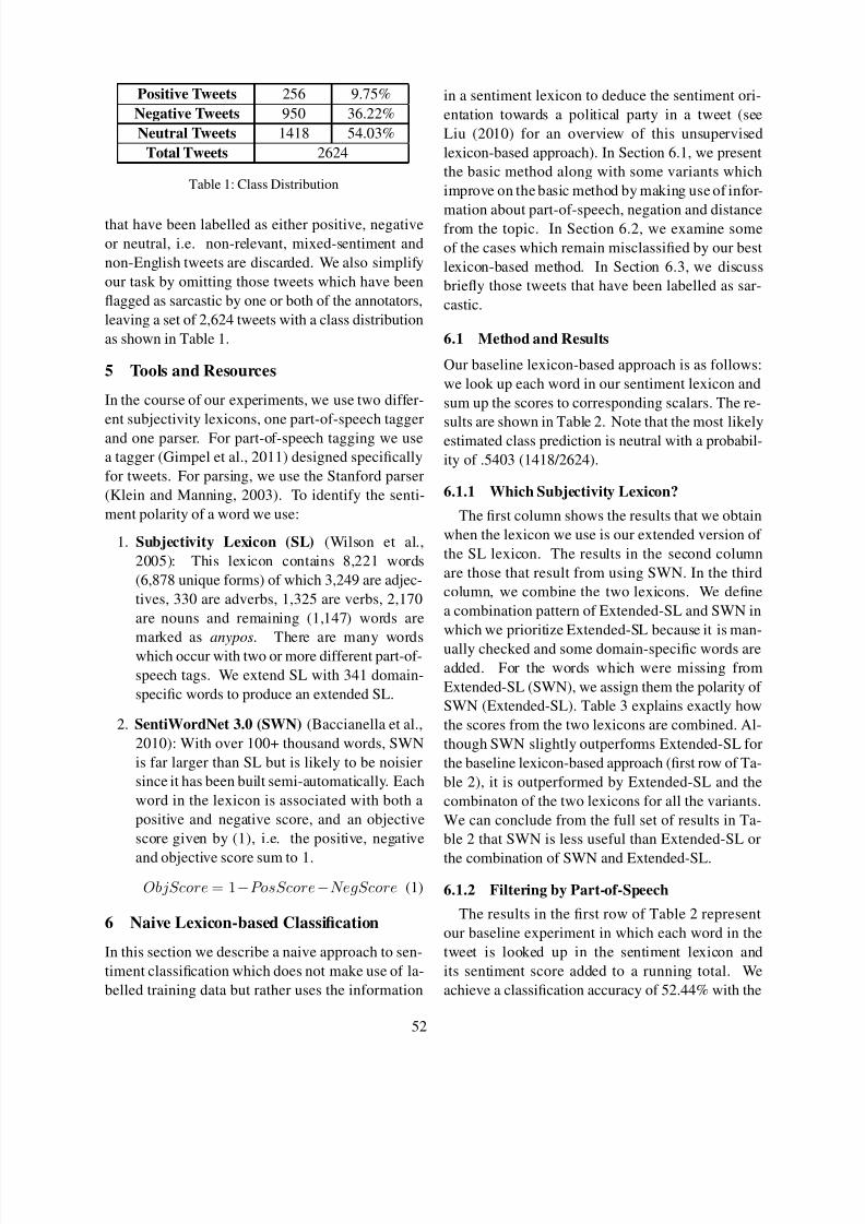
8/13/2019 Workshop on Language Analysis in Social Media
http://slidepdf.com/reader/full/workshop-on-language-analysis-in-social-media 62/101

8/13/2019 Workshop on Language Analysis in Social Media
http://slidepdf.com/reader/full/workshop-on-language-analysis-in-social-media 63/101
Method Extended-SL SWN Combined
3-Class Classification (Pos vs
Neg vs Neu) Correct Accuracy Correct Accuracy Correct Accuracy
Baseline 1376 52.44% 1379 52.55% 1288 49.09%
Baseline + Adj 1457 55.53% 1449 55.22% 1445 55.07%
Baseline + Adj + S 1480 56.40% 1459 55.60% 1481 56.44%
Baseline + Adj + S + Neg 1495 56.97% 1462 55.72% 1496 57.01%Baseline + Adj + S + Neg +
Phrases 1511 57.58% 1479 56.36% 1509 57.51%
Baseline + Adj + S + Neg +
Phrases + Than 1533 58.42% 1502 57.24% 1533 58.42%
Distance Based Scoring:
Baseline + Adj + S + Neg +
Phrases + Than
1545 58.88% 1506 57.39% 1547 58.96%
Sarcastic Tweets 87/344 25.29% 81/344 23.55% 87/344 25.29%
Table 2: 3-class classification using the naive lexicon-based approach. The majority baseline is 54.03%.
Extended-
SL
polarity
SWN
Polarity
Combination
Polarity
-1 -1 -2-1 0 -1
-1 1 -1
0 -1 -0.5
0 0 0
0 1 0.5
1 -1 1
1 0 1
1 1 2
Table 3: Combination Scheme of extended-SL and SWN.
Here 0 represents either a neutral word or a word missing
from the lexicon.
Extended-SL lexicon. We speculate that this low
accuracy is occurring because too many words that
appear in the sentiment lexicon are included in the
overall sentiment score without actually contribut-
ing to the sentiment towards the topic. To refine our
approach one step further, we use part-of-speech in-
formation and consider only adjectives for the clas-
sification of tweets since adjectives are strong in-
dicators of sentiment (Hatzivassiloglou and Wiebe,
2000). We achieve an accuracy improvement of ap-
proximately three absolute points, and this improve-ment holds true for both sentiment lexicons. This
supports our hypothesis that we are using irrelevant
information for classification in the baseline system.
Our next improvement (third row of Table 2)
comes from mapping all inflected forms to their
stems (using the Porter stemmer). Examples of in-
flected forms that are reduced to their stems are de-
lighted or delightful. Using stemming with adjec-
tives over the baseline, we achieve an accuracy of
56.40% with Extended-SL.
6.1.3 Negation
“ Negation is a very common linguistic construc-
tion that affects polarity and, therefore, needs to
be taken into consideration in sentiment analysis”
(Councill et al., 2010). We perform negation han-
dling in tweets using two different approaches. In
the first approach, we first identify negation words
53

8/13/2019 Workshop on Language Analysis in Social Media
http://slidepdf.com/reader/full/workshop-on-language-analysis-in-social-media 64/101
and reverse the polarity of sentiment-bearing words
within a window of three words. In the second ap-
proach, we try to resolve the scope of the negation
using syntactic parsing. The Stanford dependency
scheme (de Marneffe and Manning, 2008) has a spe-
cial relation (neg) to indicate negation. We reverse
the sentiment polarity of a word marked via the negrelation as being in the scope of a negation. Using
the first approach, we see an improvement of 0.6%
in the classification accuracy with the Extended-SL
lexicon. Using the second approach, we see an
improvement of 0.5%. Since there appears to be
very little difference between the two approaches to
negation-handling and in order to reduce the compu-
tational burden of running the Stanford parser each
time to obtain the dependencies, we continue further
experiments with the first method only. Using base-
line + stemming + adjectives + neg we achieve an
accuracy of 56.97% with the Extended-SL lexicon.
6.1.4 Domain-specific idioms
In the context of political tweets we see many
sentiment-bearing idioms and fixed expressions, e.g.
god save us, X for Taoiseach1, wolf in sheep’s cloth-
ing, etc. In our study, we had a total of 89 phrases.
When we directly account for these phrases, we
achieve an accuracy of 57.58% (an absolute im-
provement of 0.6 points over the last step).
6.1.5 Comparative ExpressionsAnother form of expressing an opinion towards
an entity is by comparing the entity with some other
entity. For example consider the tweet:
Fast Food sounds like a better vote than Fianna Fail.(2)
In this tweet, an indirect negative sentiment is ex-
pressed towards the political party Fianna F ail. In
order to take into account such constructions, the
following procedure is applied: we divide the tweet
into two parts, left and right. The left part contains
the text which comes before the than and the right
part contains the text which comes after than, e.g.
Tweet: ‘X is better than Y’
Left: ‘X is better’
Right: ‘Y’.
1The term Taoiseach refers to the Irish Prime Minister.
We then use the following strategy to calculate the
polarity of the tweet oriented towards the entity:
S left = sentiment score of Left.
S right = sentiment score of Right.
Ent pos left = if entity is left of
‘than
, then 1, otherwise − 1.Ent pos right = if entity is right of
‘than, then 1, otherwise − 1.
S (tweet) = Ent pos left ∗ S left +
Ent pos right ∗ S right. (3)
So in (2) above the entity, Fianna F´ ail, is to the
right of than meaning that its Ent pos right value
is 1 and its Ent pos left value is -1. This has the
effect of flipping the polarity of the positive word
better . By including the “than” comparison, we see
an improvement of absolute 0.8% (third last row of Table 2).
6.1.6 Distance Scoring
To emphasize the topic-oriented nature of our sen-
timent classification, we also define a distance-based
scoring function where we define the overall score
of the tweet as given in (4). Here dis(word) is de-
fined as number of words between the topic (i.e. the
political entity) and the sentiment word.
S (tweet) =n
i=1
S (wordi)/dis(wordi). (4)
The addition of the distance information further en-
hanced our system accuracy by 0.45%, taking it to
58.88% (second last row of Table 2). Our highest
overall accuracy (58.96) is achieved in this setting
using the combined lexicon.
It should be noted that this lexicon-based ap-
proach is overfitting to our dataset since the list of
domain-specific phrases and the form of the com-
parative constructions have been obtained from the
dataset itself. This means that we are making a
strong assumption about the representativeness of this dataset and accuracy on a held-out test set is
likely to be lower.
6.2 Error Analysis
In this section we discuss pitfalls of the naive
lexicon-based approach with the help of some exam-
ples (see Table 4). Consider the first example from
54

8/13/2019 Workshop on Language Analysis in Social Media
http://slidepdf.com/reader/full/workshop-on-language-analysis-in-social-media 65/101
the table, @username and u believe people in fianna
fail . What are you a numbskull or a journalist ?
In this tweet, we see that negative sentiment is im-
parted by the question part of the tweet, but actually
there are no sentiment adjectives. The word numb-
skull is contributing to the sentiment but is tagged as
a noun and not as an adjective. This tweet is taggedas negative by our annotators and as neutral by our
lexicon-based classifier.
Consider the second example from Table 4,
@username LOL . A guy called to our house tonight
selling GAA tickets . His first words were : I’m
not from Fianna Fail . This is misclassified because
there are no sentiment bearing words according to
the sentiment lexicon. The last tweet in the table rep-
resents another example of the same problem. Note
however that the emoticon :/ in the last tweet and the
web acronym LOL in the second tweet are providing
hints which our system is not making use of.
In the third example from Table 4, @username
Such scary words .’ Sinn Fein could top the poll ’
in certain constituencies . I feel sick at the thought
of it . ’ In this example, we have three sentiment
bearing words: scary, top and sick . Two of the three
words are negative and one word is positive. The
word scary is stemmed incorrectly as scari which
means that it is out of the scope of our lexicons.
If we just count the number of sentiment words re-
maining, then this tweet is labelled as neutral but ac-
tually is negative with respect to the party Sinn F ein.We proposed the use of distance as a measure of re-
latedness to the topic and we observed a minor im-
provement in classification accuracy. However, for
this example, the distance-based approach does not
work. The word top is just two words away from the
topic and thus contributes the maximum, resulting in
the whole tweet being misclassified as positive.
6.3 Sarcastic Tweets
“Political discouse is plagued with humor, double
entendres, and sarcasm; this makes determining po-litical preference of users hard and inferring voting
intention even harder.”(Gayo-Avello, 2012)
As part of the annotation process, annotators were
asked to indicate whether they thought a tweet ex-
hibited sarcasm. Some examples of tweets that were
annotated as sarcastic are shown in Table 5.
We made the decision to omit these tweets from
the main sentiment classification experiments under
the assumption that they constituted a special case
which would be better handled by a different clas-
sifier. This decision is vindicated by the results in
the last row of Table 2 which show what happens
when we apply our best classifier ( Distance-based
Scoring: Baseline+Adj+S+Neg+Phrases+Than) tothe sarcastic tweets – only a quarter of them are cor-
rectly classified. Even with a very large and highly
domain-tuned lexicon, the lexicon-based approach
on its own will struggle to be of use for cases such
as these, but the situation might be improved were
the lexicon to be used in conjunction with possible
sarcasm indicators such as exclamation marks.
7 Supervised Machine Learning
Although our dataset is small, we investigate
whether we can improve over the lexicon-based ap-
proach by using supervised machine learning. As
our learning algorithm, we employ support vector
machines in a 5-fold cross validation setup. The tool
we use is SVMLight (Joachims, 1999).
We explore two sets of features. The first are the
tried-and-tested unigram presence features which
have been used extensively not only in sentiment
analysis but in other text classification tasks. As we
have only 2,624 training samples, we performed fea-
ture selection by ranking the features using the Chi-
squared metric.The second feature set consists of 25 features
which are inspired by the work on lexicon-based
classification described in the previous section.
These are the counts of positive, negative, objec-
tive words according to each of the three lexicons
and the corresponding sentiment scores for the over-
all tweets. In total there are 19 such features. We
also employ six Twitter-related presence features:
positive emoticons, negative emoticons, URLs, pos-
itive hashtags, negative hashtags and neutral hash-
tags. For further reference we call this second set of features our “hand-crafted” features.
The results are shown in Table 6. We can see
that using the hand-crafted features alone barely im-
proves over the majority baseline of 54.03 but it does
improve over our baseline lexicon-based approach
(see first row of Table 2). Encouragingly, we see
some benefit from using these features in conjunc-
55
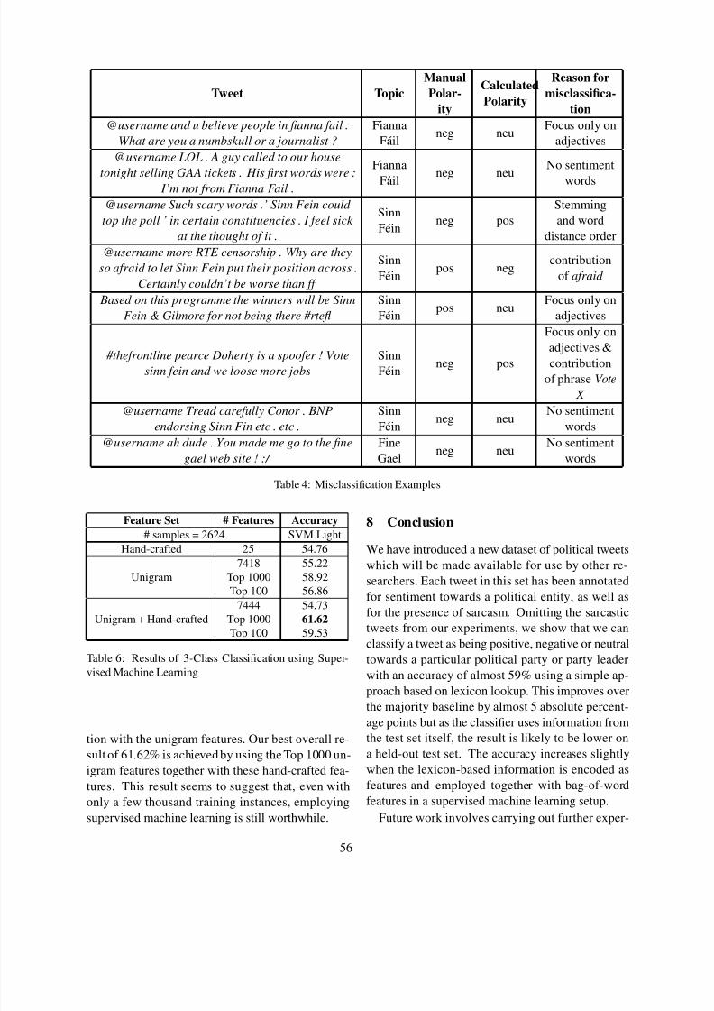
8/13/2019 Workshop on Language Analysis in Social Media
http://slidepdf.com/reader/full/workshop-on-language-analysis-in-social-media 66/101
Tweet Topic
Manual
Polar-
ity
Calculated
Polarity
Reason for
misclassifica-
tion
@username and u believe people in fianna fail .
What are you a numbskull or a journalist ?
Fianna
Fail neg neu
Focus only on
adjectives
@username LOL . A guy called to our house
tonight selling GAA tickets . His first words were : I’m not from Fianna Fail .
Fianna
Fail neg neu
No sentiment
words
@username Such scary words .’ Sinn Fein could
top the poll ’ in certain constituencies . I feel sick
at the thought of it .
Sinn
Fein neg pos
Stemming
and word
distance order
@username more RTE censorship . Why are they
so afraid to let Sinn Fein put their position across .
Certainly couldn’t be worse than ff
Sinn
Fein pos neg
contribution
of afraid
Based on this programme the winners will be Sinn
Fein & Gilmore for not being there #rtefl
Sinn
Fein pos neu
Focus only on
adjectives
#thefrontline pearce Doherty is a spoofer ! Votesinn fein and we loose more jobs
SinnFein
neg pos
Focus only on
adjectives &
contribution
of phrase Vote
X
@username Tread carefully Conor . BNP
endorsing Sinn Fin etc . etc .
Sinn
Fein neg neu
No sentiment
words
@username ah dude . You made me go to the fine
gael web site ! :/
Fine
Gael neg neu
No sentiment
words
Table 4: Misclassification Examples
Feature Set # Features Accuracy
# samples = 2624 SVM Light
Hand-crafted 25 54.76
Unigram
7418 55.22
Top 1000 58.92
Top 100 56.86
Unigram + Hand-crafted
7444 54.73
Top 1000 61.62
Top 100 59.53
Table 6: Results of 3-Class Classification using Super-
vised Machine Learning
tion with the unigram features. Our best overall re-
sult of 61.62% is achieved by using the Top 1000 un-
igram features together with these hand-crafted fea-
tures. This result seems to suggest that, even with
only a few thousand training instances, employing
supervised machine learning is still worthwhile.
8 Conclusion
We have introduced a new dataset of political tweets
which will be made available for use by other re-
searchers. Each tweet in this set has been annotated
for sentiment towards a political entity, as well as
for the presence of sarcasm. Omitting the sarcastic
tweets from our experiments, we show that we can
classify a tweet as being positive, negative or neutral
towards a particular political party or party leader
with an accuracy of almost 59% using a simple ap-
proach based on lexicon lookup. This improves over
the majority baseline by almost 5 absolute percent-age points but as the classifier uses information from
the test set itself, the result is likely to be lower on
a held-out test set. The accuracy increases slightly
when the lexicon-based information is encoded as
features and employed together with bag-of-word
features in a supervised machine learning setup.
Future work involves carrying out further exper-
56

8/13/2019 Workshop on Language Analysis in Social Media
http://slidepdf.com/reader/full/workshop-on-language-analysis-in-social-media 67/101
Sarcastic Tweets
Ah bless Brian Cowen’s little cotton socks! He’s staying on as leader of FF because its better for the
country. How selfless!
So now Brian Cowen is now Minister for foreign affairs and Taoiseach? Thats exactly what he needs
more responsibilities http://bbc.in/hJI0hb
Mary Harney is going. Surprise surprise! Brian Cowen is going to be extremely busy with all these
portfolios to administer. Super hero! Now in its darkest hour Fianna Fail needs. . . Ivor!
Labour and Fine Gael have brought the election forward by 16 days Crisis over Ireland is SAVED!! #vinb
@username Maybe one of those nice Sinn Fein issue boiler suits? #rtefl
I WILL vote for Fine Gael if they pledge to dress James O’Reilly as a leprechaun and send him
to the White House for Paddy’s Day.
Table 5: Examples of tweets which have been flagged as sarcastic
iments on those tweets that have been annotated as
sarcastic, exploring the use of syntactic dependency
paths in the computation of distance between a wordand the topic, examining the role of training set class
bias on the supervised machine learning results and
exploring the use of distant supervision to obtain
more training data for this domain.
Acknowledgements
Thanks to Emmet O Briain, Lesley Ni Bhriain andthe anonymous reviewers for their helpful com-ments. This research has been supported by En-terprise Ireland (CFTD/2007/229) and by Science
Foundation Ireland (Grant 07/CE/ I1142) as part of the CNGL (www.cngl.ie) at the School of Comput-ing, DCU.
References
Stefano Baccianella, Andrea Esuli, and Fabrizio Sebas-
tiani. 2010. Sentiwordnet 3.0: An enhanced lexical
resource for sentiment analysis and opinion mining. In
Proceedings of the Seventh International Conference
on Language Resources and Evaluation (LREC’10).
Akshat Bakliwal, Piyush Arora, Senthil Madhappan,Nikhil Kapre, Mukesh Singh, and Vasudeva Varma.
2012. Mining sentiments from tweets. In Proceedings
of the WASSA’12 in conjunction with ACL’12.
Adam Bermingham and Alan F. Smeaton. 2010. Clas-
sifying sentiment in microblogs: is brevity an advan-
tage? In Proceedings of the 19th ACM international
conference on Information and Knowledge Manage-
ment .
Adam Bermingham and Alan Smeaton. 2011. On using
Twitter to monitor political sentiment and predict elec-
tion results. In Proceedings of the Workshop on Sen-timent Analysis where AI meets Psychology (SAAIP
2011).
Nibir Nayan Bora. 2012. Summarizing public opinions
in tweets. In Journal Proceedings of CICLing 2012.
Paula Chesley. 2006. Using verbs and adjectives to au-
tomatically classify blog sentiment. In Proceedings
of AAAI-CAAW-06, the Spring Symposia on Computa-
tional Approaches.
Murphy Choy, Michelle L. F. Cheong, Ma Nang Laik,
and Koo Ping Shung. 2011. A sentiment analysis
of Singapore Presidential Election 2011 using Twitter
data with census correction. CoRR, abs/1108.5520.Isaac G. Councill, Ryan McDonald, and Leonid Ve-
likovich. 2010. What’s great and what’s not: learn-
ing to classify the scope of negation for improved sen-
timent analysis. In Proceedings of the Workshop on
Negation and Speculation in Natural Language Pro-
cessing, NeSp-NLP ’10.
Dmitry Davidov, Oren Tsur, and Ari Rappoport. 2010.
Enhanced sentiment learning using Twitter hashtags
and smileys. In Proceedings of the 23rd International
Conference on Computational Linguistics: Posters.
Marie-Catherine de Marneffe and Christopher D. Man-
ning. 2008. The stanford typed dependencies repre-
sentation. In Proceedings of the COLING Workshop
on Cross-Framework and Cross-Domain Parser Eval-
uation.
Michael Gallagher and Michael Marsh. 2011. How Ire-
land Voted 2011: The Full Story of Ireland’s Earth-
quake Election. Palgrave Macmillan.
Daniel Gayo-Avello. 2012. “I wanted to predict elec-
tions with Twitter and all I got was this lousy paper”.
57

8/13/2019 Workshop on Language Analysis in Social Media
http://slidepdf.com/reader/full/workshop-on-language-analysis-in-social-media 68/101
A balanced survey on election prediction using Twitter
data. CoRR, abs/1204.6441.
Kevin Gimpel, Nathan Schneider, Brendan O’Connor,
Dipanjan Das, Daniel Mills, Jacob Eisenstein, Michael
Heilman, Dani Yogatama, Jeffrey Flanigan, and
Noah A. Smith. 2011. Part-of-speech tagging for
Twitter: annotation, features, and experiments. In Pro-
ceedings of the 49th Annual Meeting of the Associa-tion for Computational Linguistics: Human Language
Technologies: short papers - Volume 2.
Alec Go, Richa Bhayani, and Lei Huang. 2009. Twitter
sentiment classification using distant supervision. In
CS224N Project Report, Stanford University.
Namrata Godbole, Manjunath Srinivasaiah, and Steven
Skiena. 2007. Large-scale sentiment analysis for
news and blogs. In Proceedings of the International
Conference on Weblogs and Social Media (ICWSM).
Vasileios Hatzivassiloglou and Janyce M. Wiebe. 2000.
Effects of adjective orientation and gradability on sen-
tence subjectivity. In Proceedings of COLING.
Thorsten Joachims. 1999. Advances in kernel meth-
ods. chapter Making large-scale support vector ma-
chine learning practical, pages 169–184. MIT Press,
Cambridge, MA, USA.
Dan Klein and Christopher D. Manning. 2003. Accurate
unlexicalized parsing. In Proceedings of the 41st An-
nual Meeting on Association for Computational Lin-
guistics - Volume 1.
Bing Liu. 2010. Handbook of natural language pro-
cessing. chapter Sentiment Analysis and Subjectivity.
Chapman and Hall.
Brendan O’Connor, Ramnath Balasubramanyan,
Bryan R. Routledge, and Noah A. Smith. 2010. Fromtweets to polls: Linking text sentiment to public opin-
ion time series. In Proceedings of the International
Conference on Weblogs and Social Media (ICWSM).
Alexander Pak and Patrick Paroubek. 2010. Twitter as a
corpus for sentiment analysis and opinion mining. In
Proceedings of the Seventh International Conference
on Language Resources and Evaluation (LREC’10).
Bo Pang, Lillian Lee, and Shivakumar Vaithyanathan.
2002. Thumbs up?: sentiment classification using ma-
chine learning techniques. In Proceedings of the con-
ference on Empirical Methods in Natural Language
Processing - Volume 10.
James W. Pennebaker, Cindy K. Chung, Molly Ireland,Amy Gonzales, and Roger J. Booth. 2007. The de-
velopment and psychometric properties of liwc2007.
Technical report, Austin,Texas.
Andranik Tumasjan, Timm Oliver Sprenger, Philipp G.
Sandner, and Isabell M. Welpe. 2010. Predicting elec-
tions with Twitter: What 140 characters reveal about
political sentiment. In Proceedings of the Interna-
tional Conference on Weblogs and Social Media.
Peter D. Turney. 2002. Thumbs up or thumbs down?:
semantic orientation applied to unsupervised classifi-
cation of reviews. In Proceedings of the 40th Annual
Meeting on Association for Computational Linguis-
tics.
Hao Wang, Dogan Can, Abe Kazemzadeh, Francois Bar,
and Shrikanth Narayanan. 2012. A system for real-
time Twitter sentiment analysis of 2012 U.S. presiden-tial election cycle. In ACL (System Demonstrations).
Theresa Wilson, Janyce Wiebe, and Paul Hoffmann.
2005. Recognizing contextual polarity in phrase-level
sentiment analysis. In Proceedings of the conference
on Human Language Technology and Empirical Meth-
ods in Natural Language Processing.
58

8/13/2019 Workshop on Language Analysis in Social Media
http://slidepdf.com/reader/full/workshop-on-language-analysis-in-social-media 69/101
Proceedings of the Workshop on Language in Social Media (LASM 2013), pages 59–68,Atlanta, Georgia, June 13 2013. c2013 Association for Computational Linguistics
A Case Study of Sockpuppet Detection in Wikipedia
Thamar Solorio and Ragib Hasan and Mainul Mizan
The University of Alabama at Birmingham
1300 University Blvd.Birmingham, AL 35294, USA
{solorio,ragib,mainul}@cis.uab.edu
Abstract
This paper presents preliminary results of using
authorship attribution methods for the detec-
tion of sockpuppeteering in Wikipedia. Sock-puppets are fake accounts created by malicious
users to bypass Wikipedia’s regulations. Our
dataset is composed of the comments made
by the editors on the talk pages. To overcome
the limitations of the short lengths of these
comments, we use an voting scheme to com-
bine predictions made on individual user en-
tries. We show that this approach is promising
and that it can be a viable alternative to the
current human process that Wikipedia uses to
resolve suspected sockpuppet cases.
1 Introduction
Collaborative projects in social media have become
very popular in recent years. A very successful ex-
ample of this is Wikipedia, which has emerged as the
world’s largest crowd-sourced encyclopaedia. This
type of decentralized collaborative processes are ex-
tremely vulnerable to vandalism and malicious be-
havior. Anyone can edit articles in Wikipedia and/or
make comments in article discussion pages. Reg-
istration is not mandatory, but anyone can register
an account in Wikipedia by providing only little in-formation about themselves. This ease of creating
an identity has led malicious users to create mul-
tiple identities and use them for various purposes,
ranging from block evasion, false majority opinion
claims, and vote stacking. This is an example of
the multi aliasing problem known as “The Sybil At-
tack” (Douceur, 2002). Unfortunately, Wikipedia
does not provide any facility to detect such multi-
ple identities. The current process is carried out by
humans, is very time consuming, and final resolu-
tion to cases of multiple identities is based on human
intuition. A smart sockpuppet can therefore evadedetection by using multiple IP addresses, modifying
writing style, and changing behavior. Also, a mali-
cious user can create sleeper accounts that perform
benign edits from time to time, but are used for sock-
puppetry when needed. Identifying such accounts
as sockpuppets is not obvious as these accounts may
have a long and diverse edit history.
Sockpuppets are a prevalent problem in Wikipedia,
there were close to 2,700 unique suspected cases
reported in 2012. In this paper, we present a small
scale study of automated detection of sockpuppetsbased on machine learning. We approach this
problem from the point of view of authorship attri-
bution (AA), where the task consists of analyzing a
written document to predict the true author. If we
can successfully model the editors’ unique writing
style from their comments, then we can use this
information to link the sockpuppet accounts to their
corresponding puppeteer. We focus on the content
from the talk pages since the articles edited on
Wikipedia have a fixed and very uniform style. In
contrast, we have observed that editors write in a
more free-form style during discussions carried out
on the talk pages. Our results show that a two-stage
process for the task can achieve promising results.
The contributions of this study are as follows:
• We present encouraging preliminary results on
using authorship attribution approaches for un-
59

8/13/2019 Workshop on Language Analysis in Social Media
http://slidepdf.com/reader/full/workshop-on-language-analysis-in-social-media 70/101
covering real sockpuppet cases in Wikipedia. To
the best of our knowledge, we are the first to
tackle this problem.
• We identify novel features that have high dis-
criminative power and are suitable for this task,
where the input text is very short. These features
can be helpful in other social media settings, as
there are many shared characteristics across this
genre.
The rest of the paper is organized as follows:
in Section 2, we provide a detailed discussion on
Wikipedia’s editing environment and culture. In Sec-
tion 3, we talk about authorship attribution and re-
lated work. Then in Section 4, we present our de-
tailed approach. In Sections 5, 6, and 7, we discuss
the data set, experimental setup, and results, respec-
tively. Finally, we present an overall discussion andfuture directions in Sections 8 and 9.
2 Background
In Wikipedia, whenever a user acts in bad faith, van-
dalizes existing articles, or creates spurious articles,
that user is banned from editing new content. The
ban can last for some hours, to days, and in some
cases it can be permanent. Sometimes, a banned user
creates a new account to circumvent the ban, or edits
Wikipedia without signing in.
These extra accounts or IP addresses, from whichlogged out edits are made, are called sockpuppets.
The primary (oldest) account is called the sockpup-
peteer. Whenever an editor is suspected to be a sock-
puppet of another editor, a sockpuppet investigation
case is filed against those accounts. Any editor can
file a case, but the editor must provide supporting evi-
dence as well. Typical evidence includes information
about the editing actions related to those accounts,
such as the articles, the topics, vandalism patterns,
timing of account creation, timing of edits, and voting
pattern in disagreements.Sometime after the case is filed, an administrator
will investigate the case. An administrator is an editor
with privileges to make account management deci-
sions, such as banning an editor. If the administrator
is convinced that the suspect is a sockpuppet, he de-
clares the verdict as confirmed. He also issues bans
to the corresponding accounts and closes the case.
If an administrator cannot reach a verdict on a case,
he asks for a check user to intervene. Check users
are higher privileged editors, who have access to pri-
vate information regarding editors and edits, such as
the IP address from which an editor has logged in.
Other interested editors in the case, or the original
editor who filed the case can also ask for a check user to intervene. The check user will review the ev-
idence, as well as private information regarding the
case, and will try to establish the connection between
the sockpuppet and puppeteer. Then the check user
will rule on the case. Finally, another administrator
will look at the check user report and issue a final
verdict. During the process, the accused editors, both
the puppeteer and the sockpuppet, can submit evi-
dence in their favor. But this additional evidence is
not mandatory.
The current process to resolve suspected cases of
sockpuppets has several disadvantages. We have al-
ready mentioned the first one. Because it is a manual
process, it is time consuming and expensive. Perhaps
a more serious weakness is the fact that relaying on
IP addresses is not robust, as simple counter mea-
sures can fool the check users. An alternative to this
process could be an automated framework that re-
lies on the analysis of the comments to link editor
accounts, as we propose in this paper.
3 Related Work
Modern approaches to AA typically follow a text
classification framework where the classes are the
set of candidate authors. Different machine learning
algorithms have been used, including memory-based
learners (Luyckx and Daelemans, 2008a; Luyckx
and Daelemans, 2010), Support Vector Machines
(Escalante et al., 2011), and Probabilistic Context
Free Grammars (Raghavan et al., 2010).
Similarity-based approaches have also been suc-
cessfully used for AA. In this setting, the training
documents from the same author are concatenatedinto a single file to generate profiles from author-
specific features. Then authorship predictions are
based on similarity scores. (Keselj et al., 2003; Sta-
matatos, 2007; Koppel et al., 2011) are examples of
successful examples of this approach.
Previous research has shown that low-level fea-
tures, such as character n-grams are very powerful
60

8/13/2019 Workshop on Language Analysis in Social Media
http://slidepdf.com/reader/full/workshop-on-language-analysis-in-social-media 71/101
discriminators of writing styles. Although, enriching
the models with other types of features can boost
accuracy. In particular, stylistic features (punctuation
marks, use of emoticons, capitalization information),
syntactic information (at the part-of-speech level and
features derived from shallow parsing), and even se-
mantic features (bag-of-words) have shown to beuseful.
Because of the difficulties in finding data from
real cases, most of the published work in AA eval-
uates the different methods on data collections that
were gathered originally for other purposes. Exam-
ples of this include the Reuters Corpus (Lewis et al.,
2004) that has been used for benchmarking different
approaches to AA (Stamatatos, 2008; Plakias and
Stamatatos, 2008; Escalante et al., 2011) and the
datasets used in the 2011 and 2012 authorship identi-
fication competitions from the PAN Workshop series
(Argamon and Juola, 2011; Juola, 2012). Other re-
searchers have invested efforts in creating their own
AA corpus by eliciting written samples from subjects
participating in their studies (Luyckx and Daelemans,
2008b; Goldstein-Stewart et al., 2008), or crawling
though online websites (Narayanan et al., 2012).
In contrast, in this paper we focus on data from
Wikipedia, where there is a real need to identify if
the comments submitted by what appear to be dif-
ferent users, belong to a sockpuppeteer. Data from
real world scenarios like this make solving the AA
problem an even more urgent and practical matter,but also impose additional challenges to what is al-
ready a difficult problem. First, the texts analyzed in
the Wikipedia setting were generated by people with
the actual intention of deceiving the administrators
into believing they are indeed coming from differ-
ent people. With few exceptions (Afroz et al., 2012;
Juola and Vescovi, 2010), most of the approaches to
AA have been evaluated with data where the authors
were not making a conscious effort to deceive or dis-
guise their own identities or writeprint. Since there
has been very little research done on deception detec-tion, it is not well understood how AA approaches
need to be adapted for these situations, or what kinds
of features must be included to cope with deceptive
writing. However, we do assume this adds a com-
plicating factor to the task, and previous research
has shown considerable decreases in AA accuracy
when deception is present (Brennan and Greenstadt,
2009). Second, the length of the documents is usu-
ally shorter for the Wikipedia comments than that of
other collections used. Document length will clearly
affect the prediction performance of AA approaches,
as the shorter documents will contain less informa-
tion to develop author writeprint models and to make
an inference on attribution. As we will describe later,this prompted us to reframe our solution in order to
circumvent this short document length issue. Lastly,
the data available is limited, there is an average of 80
entries per user in the training set from the collection
we gathered, and an average of 8 messages in the test
set, and this as well limits the amount of evidence
available to train author models. Moreover, the test
cases have an average of 8 messages. This is a very
small amount of texts to make the final prediction.
4 Approach
In our framework, each comment made by a user is
considered a “document” and therefore, each com-
ment represents an instance of the classification task.
There are two steps in our method. In the first step,
we gather predictions from the classifier on each com-
ment. Then in the second step we take the predictions
for each comment and combine them in a majority
voting schema to assign final decisions to each ac-
count.
The two step process we just described helps us
deal with the challenging length of the individualcomments. It is also an intuitive approach, since what
we need to determine is if the account belongs to the
sockpuppeteer. The ruling is at the account-level,
which is also consistent with the human process. In
the case of a positive prediction by our system, we
take as a confidence measure on the predictions the
percentage of comments that were individually pre-
dicted as sockpuppet cases.
4.1 Feature Engineering
In this study, we have selected typical features of authorship attribution, as well as new features we
collected from inspecting the data by hand. In total,
we have 239 features that capture stylistic, grammati-
cal, and formatting preferences of the authors. The
features are described below.
Total number of characters: The goal of this
feature is to model the author’s behavior of writing
61

8/13/2019 Workshop on Language Analysis in Social Media
http://slidepdf.com/reader/full/workshop-on-language-analysis-in-social-media 72/101
long wordy texts, or short comments.
Total number of sentences: We count the total
number of sentences in the comments. While this fea-
ture is also trying to capture some preferences regard-
ing the productivity of the author’s comments, it can
tell us more about the author’s preference to organize
the text in sentences. Some online users tend to writein long sentences and thus end up with a smaller num-
ber of sentences. To fragment the comments into sen-
tences, we use the Lingua-EN-Sentence-0.25 from
www.cpan.org (The Comprehensive Perl Archive
Network). This off-the-shelf tool prevents abbrevia-
tions to be considered as sentence delimiters.
Total number of tokens: We define a token as
any sequence of consecutive characters with no white
spaces in between. Tokens can be words, numbers,
numbers with letters, or with punctuation, such as
apple, 2345, 15th, and wow!!!. For this feature we
just count how many tokens are in the comment.
Words without vowels: Most English words have
one or more vowels. The rate of words without vow-
els can also be a giveaway marker for some authors.
Some words without vowels are try, cry, fly, myth,
gym, and hymn.
Total alphabet count: This feature consists of
the count of all the alphabetic characters used by the
author in the text.
Total punctuation count: Some users use punctu-
ation marks in very unique ways. For instance, semi-
colons and hyphens show noticeable differences intheir use, some people avoid them completely, while
others might use them in excess. Moreover, the use
of commas is different in different parts of the world,
and that too can help identify the author.
Two/three continuous punctuation count: Se-
quences of the same punctuation mark are often used
to emphasize or to add emotion to the text, such as
wow!!!, and really??. Signaling emotion in written
text varies greatly for different authors. Not every-
one displays emotions explicitly or feels comfortable
expressing them in text. We believe this could alsohelp link users to sockpuppet cases.
Total contraction count: Contractions are used
for presenting combined words such as don’t , it’s,
I’m, and he’s. The contractions, or the spelled-out-
forms are both correct grammatically. Hence, the use
of contraction is somewhat a personal writing style
attribute. Although the use of contractions varies
across different genres, in social media they are com-
monly used.
Parenthesis count: This is a typical authorship at-
tribution feature that depicts the rate at which authors
use parenthesis in their comments.
All caps letter word count: This is a feature
where we counted the number of tokens having allupper case letters. They are either abbreviations, or
words presented with emphasis. Some examples are
USA, or “this is NOT correct”.
Emoticons count: Emoticons are pictorial rep-
resentations of feelings, especially facial expres-
sions with parenthesis, punctuation marks, and letters.
They typically express the author’s mood. Some com-
monly used emoticons are :) or :-) for happy face, :(
for sad face, ;) for winking, :D for grinning,<3 for
love/heart, :O for being surprised, and :P for being
cheeky/tongue sticking out.
Happy emoticons count: As one of the most
widely used emoticons, happy face was counted as a
specific feature. Both :) and :-) were counted towards
this feature.
Sentence count without capital letter at the be-
ginning: Some authors start sentences with numbers
or small letters. This feature captures that writing
style. An example can be “1953 was the year, ...” or,
“big, bald, and brass - all applies to our man”.
Quotation count: This is an authorship attribu-
tion feature where usage of quotation is counted as
a feature. When quoting, not everyone uses the quo-tation punctuation and hence quotation marks count
may help discriminate some writers from others.
Parts of speech (POS) tags frequency: We took
a total of 36 parts of speech tags from the Penn Tree-
bank POS (Marcus et al., 1993) tag set into considera-
tion. We ignored all tags related to punctuation marks
as we have other features capturing these characters.
Frequency of letters: We compute the frequency
of each of the 26 English letters in the alphabet. The
count is normalized by the total number of non-white
characters in the comment. This contributed 26 fea-tures to the feature set.
Function words frequency: It has been widely
acknowledged that the rate of function words is a
good marker of authorship. We use a list of function
words taken from the function words in (Zheng et
al., 2006). This list contributed 150 features to the
feature set.
62

8/13/2019 Workshop on Language Analysis in Social Media
http://slidepdf.com/reader/full/workshop-on-language-analysis-in-social-media 73/101
All the features described above have been used
in previous work on AA. Following are the features
that we found by manually inspecting the Wikipedia
data set. All the features involving frequency counts
are normalized by the length of the comment.
Small “i” frequency: We found the use of small
“i” in place of capital “I” to be common for someauthors. Interestingly, authors who made this mistake
repeated it quite often.
Full stop without white space frequency: Not
using white space after full stop was found quite
frequently, and authors repeated it regularly.
Question frequency: We found that some authors
use question marks more frequently than others. This
is an idiosyncratic feature as we found some authors
abuse the use of question marks for sentences that do
not require question marks, or use multiple question
marks where one question mark would suffice.Sentence with small letter frequency: Some au-
thors do not start a sentence with the first letter cap-
italized. This behavior seemed to be homogeneous,
meaning an author with this habit will do it almost
always, and across all of its sockpuppet accounts.
Alpha, digit, uppercase, white space, and tab
frequency: We found that the distribution of these
special groups of characters varies from author to
author. It captures formatting preferences of text
such as the use of “one” and “zero” in place of “1”
and “0”, and uppercase letters for every word.
‘A’, and an error frequency: Error with usage
of “a”, and “an” was quite common. Many authors
tend to use “a” in place of “an”, and vice versa. We
used a simple rate of all “a” in front of words starting
with vowel, or “an” in front of words starting with
consonant.
“he”, and “she” frequency: Use of “he”, or “she”
is preferential to each author. We found that the use of
“he”, or “she” by any specific author for an indefinite
subject is consistent across different comments.
5 Data
We collected our data from cases filed by real users
suspecting sockpupeteering in the English Wikipedia.
Our collection consists of comments made by the
accused sockpuppet and the suspected puppeteer in
various talk pages. All the information about sock-
puppet cases is freely available, together with infor-
Class Total Avg. Msg.
Train
Avg. Mesg.
Test
Sockpuppet 41 88.75 8.5
Non-sockpuppet 36 77.3 7.9
Table 1: Distribution of True/False sockpuppet cases in
the experimental data set. We show the average number
of messages in train and test partitions for both classes.
mation about the verdict from the administrators. For
the negative examples, we also collected comments
made by other editors in the comment threads of the
same talk pages. For each comment, we also col-
lected the time when the comment was posted as
an extra feature. We used this time data to investi-
gate if non-authorship features can contribute to the
performance of our model, and to compare the perfor-
mance of stylistic features and external user account
information.Our dataset has two types of cases: confirmed
sockpuppet, and rejected sockpuppet. The confirmed
cases are those where the administrators have made fi-
nal decisions, and their verdict confirmed the case as
a true sockpuppet case. Alternatively, for the rejected
sockpuppet cases, the administrator’s verdict exoner-
ates the suspect of all accusations. The distribution
of different cases is given in Table 1.
Of the cases we have collected, one of the notable
puppeteers is “-Inanna-”. This editor was active in
Wikipedia for a considerable amount of time, fromDecember 2005 to April 2006. He also has a number
of sockpuppet investigation cases against him. Ta-
ble 2 shows excerpts from comments made by this
editor on the accounts confirmed as sockpuppet. We
highlight in boldface the features that are more no-
ticeable as similar patterns between the different user
accounts.
An important aspect of our current evaluation
framework is the preprocessing of the data. We
“cleansed” the data by removing content that was
not written by the editor. The challenge we face isthat Wikipedia does not have a defined structure for
comments. We can get the difference of each modifi-
cation in the history of a comment thread. However,
not all modifications are comments. Some can be
reverts (changing content back to an old version), or
updates. Additionally, if an editor replies to more
than one part of a thread in response to multiple com-
63

8/13/2019 Workshop on Language Analysis in Social Media
http://slidepdf.com/reader/full/workshop-on-language-analysis-in-social-media 74/101
Comment from the sockpuppeteer: -Inanna-
Mine was original and i have worked on it more than 4 hours.I have changed
it many times by opinions.Last one was accepted by all the users(except for
khokhoi).I have never used sockpuppets.Please dont care Khokhoi,Tombseye
and Latinus.They are changing all the articles about Turks.The most important
and famous people are on my picture.
Comment from the sockpuppet: Altau
Hello.I am trying to correct uncited numbers in Battle of Sarikamis and CrimeanWar by resources but khoikhoi and tombseye always try to revert them.Could
you explain them there is no place for hatred and propagandas, please?
Comment from the others: Khoikhoi
Actually, my version WAS the original image. Ask any other user. Inanna’s
image was uploaded later, and was snuck into the page by Inanna’s sockpuppet
before the page got protected. The image has been talked about, and people
have rejected Inanna’s image (see above).
Table 2: Sample excerpt from a single sockpuppet case. We show in boldface some of the stylistic features shared
between the sockpuppeter and the sockpuppet.
System P R F A (%)
B-1 0.53 1 0.69 53.24
B-2 0.53 0.51 0.52 50.64
Our System 0.68 0.75 0.72 68.83
Table 3: Prediction performance for sockpuppet detec-
tion. Measures reported are Precision (P), Recall (R),
F-measure (F), and Accuracy (A). B-1 is a simple baseline
of the majority class and B-2 is a random baseline.
ments, or edits someone else’s comments for any
reason, there is no fixed structure to distinguish each
action. Hence, though our initial data collector tool
gathered a large volume of data, we could not use all
of it as the preprocessing step was highly involved
and required some manual intervention.
6 Experimental Setting
We used Weka (Witten and Frank, 2005) – a widely
recognized free and open source data-mining tool, to
perform the classification. For the purpose of this
study, we chose Weka’s implementation of Support
Vector Machine (SVM) with default parameters.
To evaluate in a scenario similar to the real settingin Wikipedia, we process each sockpuppet case sepa-
rately, we measure prediction performance, and then
aggregate the results of each case. For example, we
take data from a confirmed sockpuppet case and gen-
erate the training and test instances. The training data
comes from the comments made by the suspected
sockpuppeteer, while the test data comes from the
comments contributed by the sockpuppet account(s).We include negative samples for these cases by col-
lecting comments made on the same talk pages by
editors not reported or suspected of sockpuppeteer-
ing. Similarly, to measure the false positive ratio of
our approach, we performed experiments with con-
firmed non-sockpuppet editors that were also filed as
potential sockpuppets in Wikipedia.
7 Results
The results of our experiments are shown in Table 3.
For comparison purposes we show results of twosimple baseline systems. B-1 is the trivial classifier
that predicts every case as sockpuppet (majority). B-
2 is the random baseline (coin toss). However as seen
in the table, both baseline systems are outperformed
by our system that reached an accuracy of 68%. B-1
reached an accuracy of 53% and B-2 of 50%.
For the miss-classified instances of confirmed
sockpuppet cases, we went back to the original com-
ment thread and the investigation pages to find out
the sources of erroneous predictions for our system.
We found investigation remarks for 4 cases. Of these4 cases, 2 cases were tied on the predictions for the
individual comments. We flip a coin in our system
to break ties. From the other 2 cases, one has the
neutral comment from administrators: “Possible”,
which indicates some level of uncertainty. The last
one has comments that indicate a meat puppet. A
meat puppet case involves two different real people
64

8/13/2019 Workshop on Language Analysis in Social Media
http://slidepdf.com/reader/full/workshop-on-language-analysis-in-social-media 75/101
where one is acting under the influence of the other.
A reasonable way of taking advantage of the current
system is to use the confidence measure to make pre-
dictions of the cases where our system has the highest
confidence, or higher than some threshold, and let
the administrators handle those cases that are more
difficult for an automated approach.We have also conducted an experiment to rank our
feature set with the goal of identifying informative
features. We used information gain as the ranking
metric. A snapshot of the top 30 contributing fea-
tures according to information gain is given in Ta-
ble 4. We can see from the ranking that some of the
top-contributing features are idiosyncratic features.
Such features are white space frequency, beginning
of the sentence without capital letter, and no white
space between sentences. We can also infer from
Table 4 that function word features (My, me, its, that,
the, I, some, be, have, and since), and part of speech
tags (VBG-Verb:gerund or present participle, CD-
Cardinal number, VBP-Verb:non-3rd person singular
present, NNP-Singular proper noun, MD-Modal, and
RB-Adverb) are among the most highly ranked fea-
tures. Function words have been identified as highly
discriminative features since the earliest work on au-
thorship attribution.
Finally, we conducted experiments with two edit
timing features for 49 cases. These two features are
edit time of the day in a 24 hour clock, and edit
day of the week. We were interested in exploring if
adding these non-stylistic features could contribute
to classification performance. To compare perfor-
mance of these non-authorship attribution features,
we conducted the same experiments without these
features. The results are shown in Table 5. We can
see that average confidence of the classification, as
well as F-measure goes up with the timing features.
These timing features are easy to extract automati-
cally, therefore they should be included in an auto-
mated approach like the one we propose here.
8 Discussion
The experiments presented in the previous section are
encouraging. They show that with a relatively small
set of automatically generated features, a machine
learning algorithm can identify, with a reasonable per-
formance, the true cases of sockpuppets in Wikipedia.
Features
Whitespace frequency
Punctuation count
Alphabet count
Contraction count
Uppercase letter frequencyTotal characters
Number of tokens
me
my
its
that
Beginning of the sentence without capital letter †VBG-Verb:gerund or present participle
No white space between sentences †the
Frequency of LI
CD-Cardinal number
Frequency of F
VBP-Verb:non-3rd person singular present
Sentence start with small letter †some
NNP-Singular proper noun
be
Total Sentences
MD-Modal
? mark frequencyhave
since
RB-Adverb
Table 4: Ranking of the top 30 contributing features for the
experimental data using information gain. Novel features
from our experiment are denoted by †.
Features used Confidence F -measure
All + timing features 84.04% 0.72
All - timing features 78.78% 0.69
Table 5: Experimental result showing performance of the
method with and without timing features for the problem
of detecting sockpuppet cases. These results are on a
subset of 49 cases.
65

8/13/2019 Workshop on Language Analysis in Social Media
http://slidepdf.com/reader/full/workshop-on-language-analysis-in-social-media 76/101
7 2 7 4
7 6 7 8 8 0 8 2 8 4 8 6
C o n f i d e n c e i n %
0 . 6 5
0 . 6 6
0 . 6 7
0 . 6 8
0 . 6 9
0 . 7 0
0 . 7 1
0 . 7 2
0 . 7 3
a
b
c
d
e
f
g
Figure 1: A plot of confidence in % for successful cases vs. F-measure for the system where we remove one feature
group at a time. Here marker a) represents performance of the system with all the features. Markers b) timing features, c)
part of speech tags, d) idiosyncratic features, e) function words, f) character frequencies, and g) AA features, represent
performance of the system when the specified feature group is removed.
Since falsely accusing someone of using a sockpup-
pet could lead to serious credibility loss for users,
we believe a system like ours could be used as a first
pass in resolving the suspected sockpuppet cases, and
bring into the loop the administrators for those cases
where the certainty is not high.
To further investigate the contribution of different
groups of features in our feature set, we conducted
additional experiments where we remove one feature
group at a time. Our goal is to see which feature
group causes larger decreases in prediction perfor-
mance when it is not used in the classification. We
split our feature set into six groups, namely timing
features, parts of speech tags, idiosyncratic features,
function words, character frequencies, and author-
ship attribution features. In Figure 1, we show theresult of the experiments. From the figure, we ob-
serve that function words are the most influential
features as both confidence, and F-measure showed
the largest drop when this group was excluded. The
idiosyncratic features that we have included in the
feature set showed the second largest decrease in pre-
diction performance. Timing features, and part of
speech tags have similar drops in F-measure but they
showed a different degradation pattern on the con-
fidence: part of speech tags caused the confidence
to decrease by a larger margin than the timing fea-
tures. Finally, character frequencies, and authorship
attribution features did not affect F-measure much,
but the confidence from the predictions did decrease
considerably with AA features showing the second
largest drop in confidence overall.
9 Conclusion and Future Directions
In this paper, we present a first attempt to develop an
automated detection method of sockpuppets based
solely on the publicly available comments from the
suspected users. Sockpuppets have been a bane for
Wikipedia as they are widely used by malicious usersto subvert Wikipedia’s editorial process and consen-
sus. Our tool was inspired by recent work on the
popular field of authorship attribution. It requires no
additional administrative rights (e.g., the ability to
view user IP addresses) and therefore can be used
by regular users or administrators without check user
rights. Our experimental evaluation with real sock-
66

8/13/2019 Workshop on Language Analysis in Social Media
http://slidepdf.com/reader/full/workshop-on-language-analysis-in-social-media 77/101
puppet cases from the English Wikipedia shows that
our tool is a promising solution to the problem.
We are currently working on extending this study
and improving our results. Specific aspects we would
like to improve include a more robust confidence
measure and a completely automated implementation.
We are aiming to test our system on all the cases filedin the history of the English Wikipedia. Later on, it
would be ideal to have a system like this running in
the background and pro-actively scanning all active
editors in Wikipedia, instead of running in a user
triggered mode. Another useful extension would
be to include other languages, as English is only
one of the many languages currently represented in
Wikipedia.
Acknowledgements
This research was supported in part by ONR grantN00014-12-1-0217. The authors would like to thank
the anonymous reviewers for their comments on a
previous version of this paper.
References
S. Afroz, M. Brennan, and R. Greenstadt. 2012. Detecting
hoaxes, frauds, and deception in writing style online. In
Proceedings of the 2012 IEEE Symposium on Security
and Privacy (S&P), pages 461–475. IEEE, May.
Shlomo Argamon and Patrick Juola. 2011. Overview of
the international authorship identification competitionat PAN-2011. In Proceedings of the PAN 2011 Lab Un-
covering Plagiarism, Authorship, and Social Software
Misuse, held in conjunction with the CLEF 2011 Con-
ference on Multilingual and Multimodal Information
Access Evaluation, Amsterdam.
M. Brennan and R. Greenstadt. 2009. Practical attacks
against authorship recognition techniques. In Proceed-
ings of the Twenty-First Innovative Applications of Ar-
tificial Intelligence Conference.
John Douceur. 2002. The Sybil attack. In Peter Dr-
uschel, Frans Kaashoek, and Antony Rowstron, editors,
Peer-to-Peer Systems, volume 2429 of Lecture Notes
in Computer Science, pages 251–260. Springer Berlin / Heidelberg.
H. J. Escalante, T. Solorio, and M. Montes-y Gomez.
2011. Local histograms of character n-grams for au-
thorship attribution. In Proceedings of the 49th Annual
Meeting of the Association for Computational Linguis-
tics: Human Language Technologies, pages 288–298,
Portland, Oregon, USA, June. Association for Compu-
tational Linguistics.
Jade Goldstein-Stewart, Kerri A. Goodwin, Roberta Evans
Sabin, and Ransom K. Winder. 2008. Creating and
using a correlated corpus to glean communicative com-
monalities. In Proceedings of LREC-2008, the Sixth
International Language Resources and Evaluation Con-
ference.
P. Juola and D. Vescovi. 2010. Empirical evaluation of
authorship obfuscation using JGAAP. In Proceedingsof the 3rd ACM workshop on Artificial Intelligence and
Security, pages 14–18. ACM.
Patrick Juola. 2012. An overview of the traditional author-
ship attribution subtask. In PAN 2012 Lab, Uncovering
Plagiarism, Authorship and Social Software Misuse,
held in conjunction with CLEF 2012.
V. Keselj, F. Peng, N. Cercone, and C. Thomas. 2003.
N-gram based author profiles for authorship attribution.
In Proceedings of the Pacific Association for Computa-
tional Linguistics, pages 255–264.
Moshe Koppel, Jonathan Schler, and Shlomo Argamon.
2011. Authorship attribution in the wild. Language Resources and Evaluation, 45:83–94.
David D. Lewis, Yiming Yang, Tony G. Rose, and Fan
Li. 2004. Rcv1: A new benchmark collection for text
categorization research. J. Mach. Learn. Res., 5:361–
397, December.
Kim Luyckx and Walter Daelemans. 2008a. Authorship
attribution and verification with many authors and lim-
ited data. In Proceedings of the 22nd International Con-
ference on Computational Linguistics (Coling 2008),
pages 513–520, Manchester, UK, August.
Kim Luyckx and Walter Daelemans. 2008b. Personae: a
corpus for author and personality prediction from text.In Proceedings of LREC-2008, the Sixth International
Language Resources and Evaluation Conference.
Kim Luyckx and Walter Daelemans. 2010. The effect
of author set size and data size in authorship attribu-
tion. Literary and Linguistic Computing, pages 1–21,
August.
Mitchell P. Marcus, Mary Ann Marcinkiewicz, and Beat-
rice Santorini. 1993. Building a large annotated cor-
pus of English: the Penn treebank. Comput. Linguist.,
19(2):313–330, June.
A. Narayanan, H. Paskov, N.Z. Gong, J. Bethencourt,
E. Stefanov, E.C.R. Shin, and D. Song. 2012. On thefeasibility of internet-scale author identification. In
Proceedings of the 33rd conference on IEEE Sympo-
sium on Security and Privacy, pages 300–314. IEEE.
S. Plakias and E. Stamatatos. 2008. Tensor space models
for authorship attribution. In Proceedings of the 5th
Hellenic Conference on Artificial Intelligence: Theo-
ries, Models and Applications, volume 5138 of LNCS ,
pages 239–249, Syros, Greece.
67

8/13/2019 Workshop on Language Analysis in Social Media
http://slidepdf.com/reader/full/workshop-on-language-analysis-in-social-media 78/101
Sindhu Raghavan, Adriana Kovashka, and Raymond
Mooney. 2010. Authorship attribution using proba-
bilistic context-free grammars. In Proceedings of the
48th Annual Meeting of the ACL 2010, pages 38–42,
Uppsala, Sweden, July. Association for Computational
Linguistics.
E. Stamatatos. 2007. Author identification using imbal-
anced and limited training texts. In Proceedings of the
18th International Workshop on Database and Expert
Systems Applications, DEXA ’07 , pages 237–241, Sept.
E. Stamatatos. 2008. Author identification: Using text
sampling to handle the class imbalance problem. Infor-
mation Processing and Managemement , 44:790–799.
I. H. Witten and E. Frank. 2005. Data Mining: Practi-
cal Machine Learning Tools and Techniques. Morgan
Kauffmann, 2nd edition.
Rong Zheng, Jiexun Li, Hsinchun Chen, and Zan Huang.
2006. A framework for authorship identification of
online messages: Writing-style features and classifica-tion techniques. Journal of the American Society for
Information Science and Technology, 57(3):378–393.
68

8/13/2019 Workshop on Language Analysis in Social Media
http://slidepdf.com/reader/full/workshop-on-language-analysis-in-social-media 79/101
Proceedings of the Workshop on Language in Social Media (LASM 2013), pages 69–79,Atlanta, Georgia, June 13 2013. c2013 Association for Computational Linguistics
Towards the Detection of Reliable Food-Health Relationships
Michael Wiegand and Dietrich Klakow
Spoken Language Systems
Saarland University
D-66123 Saarbrucken, Germany
{Michael.Wiegand|Dietrich.Klakow}@lsv.uni-saarland.de
Abstract
We investigate the task of detecting reli-
able statements about food-health relation-
ships from natural language texts. For that
purpose, we created a specially annotatedweb corpus from forum entries discussing the
healthiness of certain food items. We ex-
amine a set of task-specific features (mostly)
based on linguistic insights that are instrumen-
tal in finding utterances that are commonly
perceived as reliable. These features are in-
corporated in a supervised classifier and com-
pared against standard features that are widely
used for various tasks in natural language pro-
cessing, such as bag of words, part-of speech
and syntactic parse information.
1 Introduction
In this paper, we explore some linguistic high-level
features to detect food-health relationships in natural
language texts that are perceived reliable. By food-
health relationships we mean relations that claim
that a food item is suitable (1) or unsuitable (2) for
some particular health condition.
(1) Baking soda is an approved remedy against
heartburn.
(2) During pregnancy women should not consume
any alcohol.
The same health claim may be uttered in differ-
ent ways (3)-(5) and, as a consequence, may be per-
ceived and judged differently. For the automatic ex-
traction of health claims, we believe that statements
that are perceived as reliable (4)-(5) are the most im-
portant to retrieve.
(3) Eggs do not have a negative impact on people
suffering from heart diseases.
(4) According to a leading medical scientist, the
consumption of eggs does not have a negative
impact on people suffering from heart diseases.(5) I’m suffering from a heart disease and all my
life I’ve been eating many eggs; it never had
any impact on my well-being.
In this work, we will mine a web corpus of fo-
rum entries for such relations. Social media are a
promising source of such knowledge as, firstly, the
language employed is not very technical and thus,
unlike medical texts, accessible to the general pub-
lic. Secondly, social media can be considered as an
exclusive repository of popular wisdom. With re-gard to the health conditions, we can find, for ex-
ample, home remedies. Despite the fact that many
of them are not scientifically proven, there is still a
great interest in that type of knowledge. However,
even though such content is usually not subject to
any scientific review, users would appreciate an au-
tomatic assessment of the quality of each relation ex-
pressed. In this work, we attempt a first step towards
this endeavour by automatically classifying these ut-
terances with regard to reliability.
The features we examine will be (mostly) based
on linguistic insights that are instrumental in finding
utterances that are commonly perceived as reliable.
These features are incorporated in a supervised clas-
sifier and compared against standard features that
are widely used for various tasks in natural language
processing, such as bag of words, part-of speech and
syntactic parse information.
69

8/13/2019 Workshop on Language Analysis in Social Media
http://slidepdf.com/reader/full/workshop-on-language-analysis-in-social-media 80/101
Our experiments are carried out on German data.
We believe, however, that our findings carry over
to other languages since the linguistic aspects that
we address are (mostly) language universal. For the
sake of general accessibility, all examples will be
given as English translations.
2 Related Work
As far as the extraction of health relations from
social media are concerned, the prediction of epi-
demics (Fisichella et al., 2011; Torii et al., 2011;
Diaz-Aviles et al., 2012; Munro et al., 2012) has re-
cently attracted the attention of the research commu-
nity.
Relation extraction involving food items has also
been explored in the context of ontology align-
ment (van Hage et al., 2005; van Hage et al., 2006;
van Hage et al., 2010) and also as a means of knowl-
edge acquisition for virtual customer advice in a su-
permarket (Wiegand et al., 2012a).
The works most closely related to this paper are
Yang et al. (2011) and Miao et al. (2012). Both
of these works address the extraction of food-health
relationships. Unlike this work, they extract rela-
tions from scientific biomedical texts rather than so-
cial media. Yang et al. (2011) also cover the task
of strength analysis which bears some resemblance
to the task of finding reliable utterances to some ex-
tent. However, the features applied to that classifica-
tion task are only standard features, such as bag of words.
3 Data & Annotation
As a corpus for our experiments, we used a crawl
of chefkoch.de1 (Wiegand et al., 2012a) consisting
of 418, 558 webpages of food-related forum entries.
chefkoch.de is the largest web portal for food-related
issues in the German language. From this dataset,
sentences in which some food item co-occurred with
some health condition (e.g. pregnancy, diarrhoea
or flu) were extracted. (In the following, we willalso refer to these entities as target food item and
target health condition.) The food items were iden-
tified with the help of GermaNet (Hamp and Feld-
weg, 1997), the German version of WordNet (Miller
et al., 1990), and the health conditions were used
1www.chefkoch.de
from Wiegand et al. (2012b). In total, 2604 sen-
tences were thus obtained.
For the manual annotation, each target sentence
(i.e. a sentence with a co-occurrence of target food
item and health condition) was presented in combi-
nation with the two sentences immediately preced-
ing and following it. Each target sentence was man-
ually assigned two labels, one specifying the type
of suitability (§3.1) and another specifying whether
the relation expressed is considered reliable or not
(§3.2).
3.1 Types of Suitability
The suitability-label indicates whether a polar rela-
tionship holds between the target food item and the
target health condition, and if so, which. Rather than
just focusing on positive polarity, i.e. suitability,
and negative polarity, i.e. unsuitability, we consider
more fine-grained classes. As such, the suitability-
label does not provide any explicit information about
the reliability of the utterance. In principle, ev-
ery polar relationship between target food item and
health condition expressed in a text could also be
formulated in such a way that it is perceived reliable.
In this work, we will consider the suitability-label as
given. We use it as a feature in order to measure the
correlation between suitability and reliability. The
usage of fine-grained labels is to investigate whether
subclasses of suitability or unsuitability have a ten-
dency to co-occur with reliability. (In other words:we may assume differences among labels with the
same polarity type.) We define the following set of
fine-grained suitability-labels:
3.1.1 Suitable (SUIT)
SUIT encompasses all those statements in which
the consumption of the target food item is claimed to
be suitable for people affected by a particular health
condition (6). By suitable, we mean that there will
not be a negative effect on the health of a person
once he or she consumes the target food item. How-ever, this relation type does not state that the con-
sumption is likely to improve the condition of the
person either.
(6) I also got dermatitis which is why my mother
used spelt flour [instead of wheat flour]; you
don’t taste a difference.
70
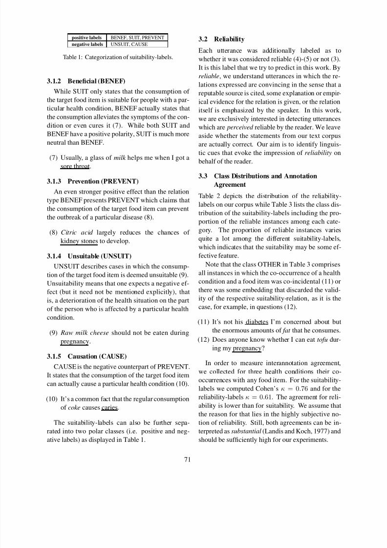
8/13/2019 Workshop on Language Analysis in Social Media
http://slidepdf.com/reader/full/workshop-on-language-analysis-in-social-media 81/101
positive labels BENEF, SUIT, PREVENT
negative labels UNSUIT, CAUSE
Table 1: Categorization of suitability-labels.
3.1.2 Beneficial (BENEF)
While SUIT only states that the consumption of
the target food item is suitable for people with a par-
ticular health condition, BENEF actually states that
the consumption alleviates the symptoms of the con-
dition or even cures it (7). While both SUIT and
BENEF have a positive polarity, SUIT is much more
neutral than BENEF.
(7) Usually, a glass of milk helps me when I got a
sore throat.
3.1.3 Prevention (PREVENT)
An even stronger positive effect than the relationtype BENEF presents PREVENT which claims that
the consumption of the target food item can prevent
the outbreak of a particular disease (8).
(8) Citric acid largely reduces the chances of
kidney stones to develop.
3.1.4 Unsuitable (UNSUIT)
UNSUIT describes cases in which the consump-
tion of the target food item is deemed unsuitable (9).
Unsuitability means that one expects a negative ef-
fect (but it need not be mentioned explicitly), that
is, a deterioration of the health situation on the part
of the person who is affected by a particular health
condition.
(9) Raw milk cheese should not be eaten during
pregnancy.
3.1.5 Causation (CAUSE)
CAUSE is the negative counterpart of PREVENT.
It states that the consumption of the target food item
can actually cause a particular health condition (10).
(10) It’s a common fact that the regular consumption
of coke causes caries.
The suitability-labels can also be further sepa-
rated into two polar classes (i.e. positive and neg-
ative labels) as displayed in Table 1.
3.2 Reliability
Each utterance was additionally labeled as to
whether it was considered reliable (4)-(5) or not (3).
It is this label that we try to predict in this work. By
reliable, we understand utterances in which the re-
lations expressed are convincing in the sense that a
reputable source is cited, some explanation or empir-ical evidence for the relation is given, or the relation
itself is emphasized by the speaker. In this work,
we are exclusively interested in detecting utterances
which are perceived reliable by the reader. We leave
aside whether the statements from our text corpus
are actually correct. Our aim is to identify linguis-
tic cues that evoke the impression of reliability on
behalf of the reader.
3.3 Class Distributions and Annotation
Agreement
Table 2 depicts the distribution of the reliability-
labels on our corpus while Table 3 lists the class dis-
tribution of the suitability-labels including the pro-
portion of the reliable instances among each cate-
gory. The proportion of reliable instances varies
quite a lot among the different suitability-labels,
which indicates that the suitability may be some ef-
fective feature.
Note that the class OTHER in Table 3 comprises
all instances in which the co-occurrence of a health
condition and a food item was co-incidental (11) or
there was some embedding that discarded the valid-ity of the respective suitability-relation, as it is the
case, for example, in questions (12).
(11) It’s not his diabetes I’m concerned about but
the enormous amounts of fat that he consumes.
(12) Does anyone know whether I can eat tofu dur-
ing my pregnancy?
In order to measure interannotation agreement,
we collected for three health conditions their co-
occurrences with any food item. For the suitability-
labels we computed Cohen’s κ = 0.76 and for the
reliability-labels κ = 0.61. The agreement for reli-
ability is lower than for suitability. We assume that
the reason for that lies in the highly subjective no-
tion of reliability. Still, both agreements can be in-
terpreted as substantial (Landis and Koch, 1977) and
should be sufficiently high for our experiments.
71

8/13/2019 Workshop on Language Analysis in Social Media
http://slidepdf.com/reader/full/workshop-on-language-analysis-in-social-media 82/101
Type Frequency Percentage
Reliable 480 18.43
Not Reliable 2124 81.57
Table 2: Distribution of the reliability-labels.
Type F requency Perc. Perc. Reliable
BENEF 502 19.28 33.39
CAUSE 482 18.51 22.57
SUIT 428 16.44 17.91
UNSUIT 277 10.64 34.05
PREVENT 74 2.84 14.04
OTHER 841 32.30 0.00
Table 3: Distribution of the suitability-labels.
4 Feature Design
4.1 Task-specific High-level Feature Types
We now describe the different task-specific high-
level feature types. We call them high-level feature
types since they model concepts that typically gen-
eralize over sets of individual words (i.e. low-level
features).
4.1.1 Explanatory Statements (EXPL)
The most obvious type of reliability is a
suitability-relation that is also accompanied by some
explanatory statement. That is, some reason for the
relation expressed is given (13). We detect reasons
by scanning a sentence for typical discourse cues
(more precisely: conjunctions) that anchor such re-
marks, e.g. which is why or because.(13) Honey has an antiseptic effect which is why it
is an ideal additive to milk in order to cure a
sore throat.
4.1.2 Frequent Observation (FREQ)
If a speaker claims to have witnessed a certain
relation very frequently or even at all times, then
there is a high likelihood that this relation actually
holds (14). We use a set of adverbs (18 expressions)
that express high frequency (e.g. often, frequently
etc.) or constancy (e.g. always, at all times etc.).
(14) What always helps me when I have the flu is a
hot chicken broth.
4.1.3 Intensifiers (INTENS)
Some utterances may also be perceived reliable if
their speaker adds some emphasis to them. One way
of doing so is by adding intensifiers to a remark (15).
(15) You can treat nausea with ginger very effec-
tively.
The intensifiers we use are a translation of the lex-
icon introduced in Wilson et al. (2005). For the de-
tection, we divide that list into two groups:
The first group INTENSsimple are unambiguous
adverbs that always function as intensifiers no mat-
ter in which context they appear (e.g. very or ex-
tremely).
The second group includes more ambiguous ex-
pressions, such as adjectives that only function as
an intensifier if they modify a polar expression
(e.g. horrible pain or terribly nice) otherwise they
function as typical polar expressions (e.g. you
are horrible− or he sang terribly−). We employ
two methods to detect these ambiguous expressions.
INTENS polar requires a polar expression of a polar-
ity lexicon to be modified by the intensifier, whileINTENSadj requires an adjective to be modified. In
order to identify polar expressions we use the polar-
ity lexicon underlying the PolArt system (Klenner
et al., 2009). We also consider adjectives since we
must assume that our polarity lexicon does not cover
all possible polar expressions. We chose adjectives
as a complement criterion as this part of speech is
known to contain most polar expressions (Hatzivas-
siloglou and McKeown, 1997; Hatzivassiloglou and
Wiebe, 2000).
4.1.4 Strong Polar Expressions (STROPO)
Instead of adding intensifiers in order to put more
emphasis to a remark (§4.1.3), one may also use
polar expressions that convey a high polar inten-
sity (16). For instance, nice and excellent refer to
the same scale and convey positive polarity but ex-
cellent has a much higher polar intensity than nice.
Taboada et al. (2011) introduced an English polar-
ity lexicon SO-CAL in which polar expressions were
also assigned an intensity label. As our German
polarity lexicon (§4.1.3) does not contain compara-
ble intensity labels, we used a German translation
of SO-CAL. We identified polar expressions with a
high intensity score (i.e. ±4 or ±5) as strong po-
lar expressions. It includes 221 highly positive and
344 highly negative polar expressions. We also dis-
tinguish the polarity type (i.e. STROPO+ refers to
positive and STROPO− refers to negative polarity).
72
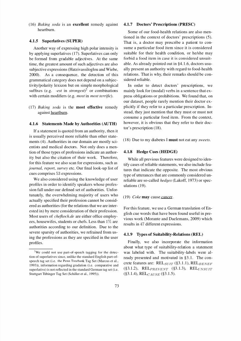
8/13/2019 Workshop on Language Analysis in Social Media
http://slidepdf.com/reader/full/workshop-on-language-analysis-in-social-media 83/101
(16) Baking soda is an excellent remedy against
heartburn.
4.1.5 Superlatives (SUPER)
Another way of expressing high polar intensity is
by applying superlatives (17). Superlatives can only
be formed from gradable adjectives. At the sametime, the greatest amount of such adjectives are also
subjective expressions (Hatzivassiloglou and Wiebe,
2000). As a consequence, the detection of this
grammatical category does not depend on a subjec-
tivity/polarity lexicon but on simple morphological
suffixes (e.g. -est in strongest )2 or combinations
with certain modifiers (e.g. most in most terrific).
(17) Baking soda is the most effective remedy
against heartburn.
4.1.6 Statements Made by Authorities (AUTH)
If a statement is quoted from an authority, then it
is usually perceived more reliable than other state-
ments (4). Authorities in our domain are mostly sci-
entists and medical doctors. Not only does a men-
tion of those types of professions indicate an author-
ity but also the citation of their work. Therefore,
for this feature we also scan for expressions, such as
journal, report , survey etc. Our final look-up list of
cues comprises 53 expressions.
We also considered using the knowledge of userprofiles in order to identify speakers whose profes-
sion fall under our defined set of authorities. Unfor-
tunately, the overwhelming majority of users who
actually specified their profession cannot be consid-
ered as authorities (for the relations that we are inter-
ested in) by mere consideration of their profession.
Most users of chefkoch.de are either office employ-
ees, housewifes, students or chefs. Less than 1% are
authorities according to our definition. Due to the
severe sparsity of authorities, we refrained from us-
ing the professions as they are specified in the userprofiles.
2We could not use part-of-speech tagging for the detec-
tion of superlatives since, unlike the standard English part-of-
speech tag set (i.e. the Penn Treebank Tag Set (Marcus et al.,
1993)), information regarding gradation (i.e. comparative and
superlative) is not reflected in the standard German tag set (i.e.
Stuttgart Tubinger Tag Set (Schiller et al., 1995)).
4.1.7 Doctors’ Prescriptions (PRESC)
Some of our food-health relations are also men-
tioned in the context of doctors’ prescriptions (5).
That is, a doctor may prescribe a patient to con-
sume a particular food item since it is considered
suitable for their health condition, or he/she may
forbid a food item in case it is considered unsuit-able. As already pointed out in §4.1.6, doctors usu-
ally present an authority with regard to food-health
relations. That is why, their remarks should be con-
sidered reliable.
In order to detect doctors’ prescriptions, we
mainly look for (modal) verbs in a sentence that ex-
press obligations or prohibitions. We found that, on
our dataset, people rarely mention their doctor ex-
plicitly if they refer to a particular prescription. In-
stead, they just mention that they must or must not
consume a particular food item. From the context,however, it is obvious that they refer to their doc-
tor’s prescription (18).
(18) Due to my diabetes I must not eat any sweets.
4.1.8 Hedge Cues (HEDGE)
While all previous features were designed to iden-
tify cases of reliable statements, we also include fea-
tures that indicate the opposite. The most obvious
type of utterances that are commonly considered un-
reliable are so-called hedges (Lakoff, 1973) or spec-ulations (19).
(19) Coke may cause cancer.
For this feature, we use a German translation of En-
glish cue words that have been found useful in pre-
vious work (Morante and Daelemans, 2009) which
results in 47 different expressions.
4.1.9 Types of Suitability-Relations (REL)
Finally, we also incorporate the information
about what type of suitability-relation a statement
was labeled with. The suitability-labels were al-
ready presented and motivated in §3.1. The con-
crete features are: RELSUIT (§3.1.1), RELBENEF
(§3.1.2), RELPREVENT (§3.1.3), RELUNSUIT
(§3.1.4), RELCAUSE (§3.1.5).
73

8/13/2019 Workshop on Language Analysis in Social Media
http://slidepdf.com/reader/full/workshop-on-language-analysis-in-social-media 84/101
Suffix Description
-WNDfood context window around food item
-WNDcond context window around health condition
-TS target sentence only
-EC entire (instance) context
Table 4: Variants for the individual feature types.
4.2 Variants of Feature Types
For our feature types we examine several variants
that differ in the size of context/scope. We distin-
guish between the target sentence and the entire con-
text of an instance, i.e. the target sentence plus the
two preceding and following sentences (§3). If only
the target sentence is considered, we can also con-
fine the occurrence of a cue word to a fixed window
(comprising 5 words) either around the target food
item or the target health condition rather than con-sidering the entire sentence.
Small contexts usually offer a good precision. For
example, if a feature type occurs nearby a mention
of the target food item or health condition, the fea-
ture type and the target expression are likely to be
related to each other. The downside of such narrow
contexts is that they may be too sparse. Wide con-
texts may be better suited to situations in which a
high recall is desirable. However, ambiguous fea-
ture types may perform poorly with these contexts
as their co-occurrence with a target expression at alarge distance is likely to be co-incidental.
Table 4 lists all the variants that we use. These
variants are applied to all feature types except the
types of suitability (§4.1.9) as this label has only
been assigned to an entire target sentence.
4.3 Other Features
Table 5 lists the entire set of features that we ex-
amine in this work. The simplest classifier that we
can construct for our task is a trivial classifier that
predicts all statements as reliable statements. The
remaining features comprise bag of words, part-of-
speech and syntactic parse information. For the
latter two features, we employ the output of the
Stanford Parser for German (Rafferty and Manning,
2008).
Features Description
all trivial classifier that always predicts a reliable state-
ment
bow bag-of-words features: all words between the target
food item and target health condition and the words
immediately preceding and following each of them
pos part-of-speech features: part-of-speech sequence be-
tween target food item and health condition and tags
of the words immediately preceding and following
each of the target expressionssynt path from syntactic parse tree from target food item
to target health condition
task all task-specific high-level feature types from §4.1
with their respective variants (§4.2)
Table 5: Description of all feature sets.
5 Experiments
Each instance to be classified is a sentence in which
there is a co-occurrence of a target food item and
a target health condition along its respective con-
text sentences (§3). We only consider sentences inwhich the co-occurrence expresses an actual suit-
ability relationship between the target food item and
the target health condition, that is, we ignore in-
stances labeled with the suitability-label OTHER
(§3.3). We make this restriction as the instances
labeled as OTHER are not eligible for being reli-
able statements (Table 3). In this work, we take the
suitability-labels for granted (this allows us to easily
exclude the instances labeled as OTHER). The au-
tomatic detection of suitability-labels would require
a different classifier with a different set of featureswhose appropriate discussion would be beyond the
scope of this paper.
5.1 Comparison of the Different Task-specific
High-level Features
In our first experiment, we want to find out how
the different task-specific high-level features that we
have proposed in this work compare to each other.
More specifically, we want to find out how the in-
dividual features correlate with the utterances that
have been manually marked as reliable. For that
purpose, Table 6 shows the top 20 features accord-
ing to Chi-square feature selection computed with
WEKA (Witten and Frank, 2005). More informa-
tion regarding the computation of Chi-square statis-
tics in the context of text classification can be found
in Yang and Pederson (1997). Note that we apply
feature selection only as a means of feature compar-
74

8/13/2019 Workshop on Language Analysis in Social Media
http://slidepdf.com/reader/full/workshop-on-language-analysis-in-social-media 85/101

8/13/2019 Workshop on Language Analysis in Social Media
http://slidepdf.com/reader/full/workshop-on-language-analysis-in-social-media 86/101
ial feature while RELSUIT is clearly below. (One
may wonder why the gap in precision between those
different features is not larger. These features are
also high-recall features – we have shown this for
RELBENEF in Table 7 – so the smaller gaps may
already have a significant impact.) In plain, this
result means that a statement conveying that some
food item alleviates the symptoms of a particular
disease or even cures it (RELBENEF ) is more likely
to be an utterance that is perceived reliable rather
than statements in which the speaker merely states
that the food item is suitable given a particular health
condition (RELSUIT ). Presumably, the latter type
of suitability-relations are mostly uttered parenthet-
ically (not emphatically), or they are remarks in
which the relation is inferred, so that they are un-
likely to provide further background information. In
Sentence (20), for example, the suitability of whole-
meal products is inferred as the speaker’s father eatsthese types of food due to his diabetes. The focus
of this remark, however, is the psychic well-being of
the speaker’s father. That entire utterance does not
present any especially reliable or otherwise helpful
information regarding the relationship between dia-
betes and wholemeal products.
(20) My father suffers from diabetes and is fed up
with eating all these wholemeal products. We
are worried that he is going to fall into a de-
pression.
Having explained that the two (frequently occur-
ring) positive suitability-labels are highly ranked
features because they separate reliable from less re-
liable statements, one may wonder why we do not
find a similar behaviour on the negative suitability-
labels. The answer to this lies in the fact that there
is no similar distinction between RELBENEF and
RELSUIT among utterances expressing unsuitabil-
ity. There is no neutral negative suitability-label
similar to RELSUIT . The relation RELUNSUIT
expresses unsuitability which is usually connectedwith some deterioration in health.
5.1.3 How important are explanatory
statements for this task?
We were very surprised that the feature type to
indicate explanatory statements EXPL (§4.1.1) per-
formed very poorly (none of its variants is listed in
Feature RELSUIT all RELBENEF
Prec 17.81 26.46 33.39
Table 8: The precision of different REL-features com-
pared to the trivial classifier all that always predicts a re-
liable utterance.
Type EXPLall EXPLcue
Percentage 22.59 8.30
Table 9: Proportion of explanatory statements among re-
liable utterances (EXPLall: all reliable instances that are
explanatory statements; EXPLcue: subset of explanatory
statements that also contain a lexical cue).
Table 6) since we assumed explanatory statements
to be one of the most relevant types of utterances.
In order to find a reason for this, we manually an-
notated all reliable utterances as to whether they can
be regarded as an explanatory statement (EXPLall
)
and, if so, whether (in principle) there are lexical
cues (such as our set of conjunctions) to identify
them (EXPLcue). Table 9 shows the proportion of
these two categories among the reliable utterances.
With more than 20% being labeled as this subtype,
explanatory statements are clearly not a fringe phe-
nomenon. However, lexical cues could only be ob-
served in approximately 1/3 of those instances. The
majority of cases, such as Sentence (21), do not con-
tain any lexical cues and are thus extremely difficult
to detect.
(21) Citrus fruits are bad for dermatitis. They in-
crease the itch. Such fruits are rich in acids that
irritate your skin.
In addition, all variants of our feature type EXPL
have a poor precision (between 20 − 25%). This
means that the underlying lexical cues are too am-
biguous.
5.1.4 How important are the different
contextual scopes?
Table 6 clearly shows that the contextual scope
of a feature type matters. For example, for the fea-
ture type FREQ, the most effective scope achieves
a Chi-square score of 105.1 while the worst vari-
ant only achieves a score of 29.2. However, there
is no unique contextual scope which always outper-
forms the other variants. This is mostly due to the
76

8/13/2019 Workshop on Language Analysis in Social Media
http://slidepdf.com/reader/full/workshop-on-language-analysis-in-social-media 87/101
Feature Set Prec Rec F1
all 26.46 100.00 41.85
bow 37.14 62.44 46.45
bow+pos 36.85 57.64 44.88
bow+synt 39.05 58.01 46.58
task 35.16 72.89 47.21
bow+task 42.54 66.01 51.56∗
Table 10: Comparison of different feature sets (summary
of features is displayed in Table 5); ∗ significantly betterthan bow at p < 0.05 (based on paired t-test).
fact the different feature types have different proper-
ties. On the one hand, there are unambiguous fea-
ture types, such as AUTH, which work fine with
a wide scope. But we also have ambiguous fea-
ture types that require a fairly narrow context. A
typical example are strong (positive) polar expres-
sions (STROPO+). (Polar expressions are known
to be very ambiguous (Wiebe and Mihalcea, 2006;
Akkaya et al., 2009).)
5.2 Classification
Table 10 compares the different feature sets with
regard to extraction performance. We carry out
a 5-fold cross-validation on our manually labeled
dataset. As a classifier, we chose Support Vector
Machines (Joachims, 1999). As a toolkit, we use
SVMLight 4 with a linear kernel.
Table 10 clearly shows the strength of the high-
level features that we proposed. They do not only
represent a strong feature set on their own but they
can also usefully be combined with bag-of-words
features. Apparently, neither part-of-speech nor
parse information are predictive for this task.
5.3 Impact of Training Data
Figure 1 compares bag-of-words features and our
task-specific high-level features on a learning curve.
The curve shows that the inclusion of our task-
specific features improves performance. Interest-
ingly, with task alone we obtain a good performance
on smaller amounts of data. However, this classifieris already saturated with 40% of the training data.
From then onwards, it is more effective to use the
combination bow+task . Our high-level features gen-
eralize well which is particularly important for situ-
ations in which only few training data are available.
4http://svmlight.joachims.org
25
30
35
40
45
50
55
10 20 30 40 50 60 70 80 90 100
F
- s c o r e
Percentage of training data
bag of words (bow)task-specific high-level features (task)
combination (bow+task)
Figure 1: Learning curve of the different feature sets.
However, in situations in which large training sets
are available, we additionally need bag of words thatare able to harness more sparse but specific informa-
tion.
6 Conclusion
In this paper, we examined a set of task-specific
high-level features in order to detect food-health re-
lations that are perceived reliable. We found that,
in principle, a subset of these features that include
adverbials expressing frequent observations, state-
ments made by authorities, strong polar expressionsand intensifiers are fairly predictive and complement
bag-of-words information. We also observed a cor-
relation between some suitability-labels and relia-
bility. Moreover, the effectiveness of the different
features depends very much on the context to which
they are applied.
Acknowledgements
This work was performed in the context of the Software-
Cluster project EMERGENT. Michael Wiegand was
funded by the German Federal Ministry of Education andResearch (BMBF) under grant no. “01IC10S01”. The
authors would like to thank Stephanie Koser for annotat-
ing the dataset presented in the paper. The authors would
also like to thank Prof. Dr. Wolfgang Menzel for provid-
ing the German version of the SO-CAL polarity lexicon
that has been developed at his department.
77

8/13/2019 Workshop on Language Analysis in Social Media
http://slidepdf.com/reader/full/workshop-on-language-analysis-in-social-media 88/101
References
Cem Akkaya, Janyce Wiebe, and Rada Mihalcea. 2009.
Subjectivity Word Sense Disambiguation. In Proceed-
ings of the Conference on Empirical Methods in Nat-
ural Language Processing (EMNLP), pages 190–199,
Singapore.
Ernesto Diaz-Aviles, Avar Stewart, Edward Velasco, Ker-
stin Denecke, and Wolfgang Nejdl. 2012. Epidemic
Intelligence for the Crowd, by the Crowd. In Proceed-
ings of the International AAAI Conference on Weblogs
and Social Media (ICWSM), Dublin, Ireland.
Marco Fisichella, Avar Stewart, Alfredo Cuzzocrea, and
Kerstin Denecke. 2011. Detecting Health Events on
the Social Web to Enable Epidemic Intelligence. In
Proceedings of the International Symposium on String
Processing and Information Retrieval (SPIRE), pages
87–103, Pisa, Italy.
Birgit Hamp and Helmut Feldweg. 1997. GermaNet - a
Lexical-Semantic Net for German. In Proceedings of
ACL workshop Automatic Information Extraction and Building of Lexical Semantic Resources for NLP Ap-
plications, pages 9–15, Madrid, Spain.
Vasileios Hatzivassiloglou and Kathleen R. McKeown.
1997. Predicting the Semantic Orientation of Adjec-
tives. In Proceedings of the Conference on European
Chapter of the Association for Computational Linguis-
tics (EACL), pages 174–181, Madrid, Spain.
Vasileios Hatzivassiloglou and Janyce Wiebe. 2000. Ef-
fects of Adjective Orientation and Gradability on Sen-
tence Subjectivity. In Proceedings of the International
Conference on Computational Linguistics (COLING),
pages 299–305, Saarbrucken, Germany.
Thorsten Joachims. 1999. Making Large-Scale SVM
Learning Practical. In B. Scholkopf, C. Burges, and
A. Smola, editors, Advances in Kernel Methods - Sup-
port Vector Learning. MIT Press.
Manfred Klenner, Stefanos Petrakis, and Angela Fahrni.
2009. Robust Compositional Polarity Classification.
In Proceedings of Recent Advances in Natural Lan-
guage Processing (RANLP), pages 180–184, Borovets,
Bulgaria.
George Lakoff. 1973. Hedging: A Study in Media Crite-
ria and the Logic of Fuzzy Concepts. Journal of Philo-
sophical Logic, 2:458 – 508.
J. Richard Landis and Gary G. Koch. 1977. The Mea-surement of Observer Agreement for Categorical Data.
Biometrics, 33(1):159–174.
Mitchell P. Marcus, Beatrice Santorini, and Mary Ann
Marcinkiewicz. 1993. Building a Large Annotated
Corpus of English: The Penn Treebank. Computa-
tional Linguistics, 19(2):313–330, June. Special Issue
on Using Large Corpora.
Qingliang Miao, Shu Zhang, Bo Zhang, Yao Meng, and
Hao Yu. 2012. Extracting and Visualizing Seman-
tic Relationships from Chinese Biomedical Text. In
Proceedings of the Pacific Asia Conference on Lan-
guage, Information and Compuation (PACLIC), pages
99–107, Bali, Indonesia.
George Miller, Richard Beckwith, Christiane Fellbaum,
Derek Gross, and Katherine Miller. 1990. Introduc-tion to WordNet: An On-line Lexical Database. Inter-
national Journal of Lexicography, 3:235–244.
Roser Morante and Walter Daelemans. 2009. Learning
the Scope of Hedge Cues in Biomedical Texts. In Pro-
ceedings of the BioNLP Workshop, pages 28–36, Boul-
der, CO, USA.
Robert Munro, Lucky Gunasekara, Stephanie Nevins,
Lalith Polepeddi, and Evan Rosen. 2012. Track-
ing Epidemics with Natural Language Processing and
Crowdsourcing. In Proceedings of the Spring Sympo-
sium for Association for the Advancement of Artificial
Intelligence (AAAI), pages 52–58, Toronto, Canada.
Anna Rafferty and Christopher D. Manning. 2008. Pars-ing Three German Treebanks: Lexicalized and Un-
lexicalized Baselines. In Proceedings of the ACL
Workshop on Parsing German (PaGe), pages 40–46,
Columbus, OH, USA.
Anne Schiller, Simone Teufel, Christine Stockert, and
Christine Thielen. 1995. Vorlaufige Guidelines
fur das Tagging deutscher Textcorpora mit STTS.
Technical report, Universitat Stuttgart, Insitut fur
maschinelle Sprachverarbeitung, and Seminar fur
Sprachwissenschaft, Universitat Tubingen.
Maite Taboada, Julian Brooke, Milan Tofiloski, Kimberly
Voll, and Manfred Stede. 2011. Lexicon-Based Meth-ods for Sentiment Analysis. Computational Linguis-
tics, 37(2):267 – 307.
Manabu Torii, Lanlan Yin, Thang Nguyen, Chand T.
Mazumdar, Hongfang Liu, David M. Hartley, and
Noele P. Nelson. 2011. An exploratory study of a text
classification framework for internet-based surveil-
lance of emerging epidemics. Internal Journal of
Medical Informatics, 80(1):56–66.
Willem Robert van Hage, Sophia Katrenko, and Guus
Schreiber. 2005. A Method to Combine Linguistic
Ontology-Mapping Techniques. In Proceedings of In-
ternational Semantic Web Conference (ISWC), pages
732 – 744, Galway, Ireland. Springer.
Willem Robert van Hage, Hap Kolb, and Guus Schreiber.
2006. A Method for Learning Part-Whole Relations.
In Proceedings of International Semantic Web Con-
ference (ISWC), pages 723 – 735, Athens, GA, USA.
Springer.
Willem Robert van Hage, Margherita Sini, Lori Finch,
Hap Kolb, and Guus Schreiber. 2010. The OAEI food
78

8/13/2019 Workshop on Language Analysis in Social Media
http://slidepdf.com/reader/full/workshop-on-language-analysis-in-social-media 89/101
task: an analysis of a thesaurus alignment task. Ap-
plied Ontology, 5(1):1 – 28.
Janyce Wiebe and Rada Mihalcea. 2006. Word Sense
and Subjectivity. In Proceedings of the International
Conference on Computational Linguistics and Annual
Meeting of the Association for Computational Linguis-
tics (COLING/ACL), pages 1065–1072,Syndney, Aus-
tralia.
Michael Wiegand, Benjamin Roth, and Dietrich Klakow.
2012a. Web-based Relation Extraction for the Food
Domain. In Proceeding of the International Confer-
ence on Applications of Natural Language Process-
ing to Information Systems (NLDB), pages 222–227,
Groningen, the Netherlands. Springer.
Michael Wiegand, Benjamin Roth, Eva Lasarcyk,
Stephanie Koser, and Dietrich Klakow. 2012b. A
Gold Standard for Relation Extraction in the Food Do-
main. In Proceedings of the Conference on Language
Resources and Evaluation (LREC), pages 507–514, Is-
tanbul, Turkey.
Michael Wiegand, Manfred Klenner, and DietrichKlakow. 2013. Bootstrapping polarity classifiers with
rule-based classification. Language Resources and
Evaluation, Online First:1–40.
Theresa Wilson, Janyce Wiebe, and Paul Hoffmann.
2005. Recognizing Contextual Polarity in Phrase-level
Sentiment Analysis. In Proceedings of the Conference
on Human Language Technology and Empirical Meth-
ods in Natural Language Processing (HLT/EMNLP),
pages 347–354, Vancouver, BC, Canada.
Ian Witten and Eibe Frank. 2005. Data Mining: Practi-
cal Machine Learning Tools and Techniques. Morgan
Kaufmann Publishers, San Francisco, US.
Yiming Yang and Jan Pederson. 1997. A Comparative
Study on Feature Selection in Text Categorization. In
Proceedings the International Conference on Machine
Learning (ICML), pages 412–420, Nashville, US.
Hui Yang, Rajesh Swaminathan, Abhishek Sharma, Vi-
las Ketkar, and Jason D’Silva, 2011. Learning Struc-
ture and Schemas from Documents, volume 375 of
Studies in Computational Intelligence, chapter Min-
ing Biomedical Text Towards Building a Quantitative
Food-disease-gene Network, pages 205–225. Springer
Berlin Heidelberg.
79

8/13/2019 Workshop on Language Analysis in Social Media
http://slidepdf.com/reader/full/workshop-on-language-analysis-in-social-media 90/101
Proceedings of the Workshop on Language in Social Media (LASM 2013), pages 80–89,Atlanta, Georgia, June 13 2013. c2013 Association for Computational Linguistics
Translating Government Agencies’ Tweet Feeds:
Specificities, Problems and (a few) Solutions
Fabrizio Gotti, Philippe Langlais
{gottif,felipe}@iro.umontreal.ca
RALI-DIROUniversite de Montreal
C.P. 6128, Succ Centre-Ville
Montreal (Quebec) Canada
H3C 3J7
Atefeh Farzindar
NLP Technologies Inc.52 Le Royer
Montreal
(Quebec) Canada
H2Y 1W7
Abstract
While the automatic translation of tweets has
already been investigated in different scenar-
ios, we are not aware of any attempt to trans-late tweets created by government agencies.
In this study, we report the experimental re-
sults we obtained when translating 12 Twitter
feeds published by agencies and organizations
of the government of Canada, using a state-of-
the art Statistical Machine Translation (SMT)
engine as a black box translation device. We
mine parallel web pages linked from the U RLs
contained in English-French pairs of tweets in
order to create tuning and training material.
For a Twitter feed that would have been other-
wise difficult to translate, we report significant
gains in translation quality using this strategy.Furthermore, we give a detailed account of the
problems we still face, such as hashtag trans-
lation as well as the generation of tweets of
legal length.
1 Introduction
Twitter is currently one of the most popular online
social networking service after Facebook, and is the
fastest-growing, with the half-a-billion user mark
reached in June 2012.1
According to Twitter’s blog,no less than 65 millions of tweets are published each
day, mostly in a single language (40% in English).
This hinders the spread of information, a situation
witnessed for instance during the Arab Spring.
1http://semiocast.com/publications/
2012_07_30_Twitter_reaches_half_a_billion_
accounts_140m_in_the_US
Solutions for disseminating tweets in different
languages have been designed. One solution con-
sists in manually translating tweets, which of course
is only viable for a very specific subset of the ma-
terial appearing on Twitter. For instance, the non-profit organization Meedan 2 has been founded in or-
der to organize volunteers willing to translate tweets
written in Arabic on Middle East issues. Another
solution consists in using machine translation. Sev-
eral portals are facilitating this,3 mainly by using
Google’s machine translation API.
Curiously enough, few studies have focused on
the automatic translation of text produced within so-
cial networks, even though a growing number of
these studies concentrate on the automated process-
ing of messages exchanged on social networks. See(Gimpel et al., 2011) for a recent review of some of
them.
Some effort has been invested in translating short
text messages (SM Ss). Notably, Munro (2010) de-
scribes the service deployed by a consortium of vol-
unteer organizations named “Mission 4636” during
the earthquake that struck Haiti in January 2010.
This service routed SM Ss alerts reporting trapped
people and other emergencies to a set of volunteers
who translated Haitian Creole SM Ss into English,
so that primary emergency responders could under-stand them. In Lewis (2010), the authors describe
how the Microsoft translation team developed a sta-
tistical translation engine (Haitian Creole into En-
glish) in as little as 5 days, during the same tragedy.
2http://news.meedan.net/
3http://www.aboutonlinetips.com/
twitter-translation-tools/
80

8/13/2019 Workshop on Language Analysis in Social Media
http://slidepdf.com/reader/full/workshop-on-language-analysis-in-social-media 91/101
Jehl (2010) addresses the task of translating En-
glish tweets into German. She concludes that the
proper treatment of unknown words is of the utmost
importance and highlights the problem of producing
translations of up to 140 characters, the upper limit
on tweet lengths. In (Jehl et al., 2012), the authors
describe their efforts to collect bilingual tweets froma stream of tweets acquired programmatically, and
show the impact of such a collection on developing
an Arabic-to-English translation system.
The present study participates in the effort for the
dissemination of messages exchanged over Twitter
in different languages, but with a very narrow focus,
which we believe has not been addressed specifically
yet: Translating tweets written by government in-
stitutions. What sets these messages apart is that,
generally speaking, they are written in a proper lan-
guage (without which their credibility would pre-
sumably be hurt), while still having to be extremely
brief to abide by the ever-present limit of 140 char-
acters. This contrasts with typical social media texts
in which a large variability in quality is observed
(Agichtein et al., 2008).
Tweets from government institutions can also dif-
fer somewhat from some other, more informal so-
cial media texts in their intended audience and ob-
jectives. Specifically, such tweet feeds often attempt
to serve as a credible source of timely information
presented in a way that engages members of the
lay public. As such, translations should present a
similar degree of credibility, ease of understanding,
and ability to engage the audience as in the source
tweet—all while conforming to the 140 character
limits.
This study attempts to take these matters into ac-
count for the task of translating Twitter feeds emitted
by Canadian governmental institutions. This could
prove very useful, since more than 150 Canadian
agencies have official feeds. Moreover, while only
counting 34 million inhabitants, Canada ranks fifth
in the number of Twitter users (3% of all users) afterthe US, the UK, Australia, and Brazil.4 This cer-
tainly explains why Canadian governments, politi-
cians and institutions are making an increasing use
of this social network service. Given the need of
4http://www.techvibes.com/blog/how-
canada-stacks-up-against-the-world-on-
twitter-2012-10-17
Canadian governmental institutions to disseminate
information in both official languages (French and
English), we see a great potential value in targeted
computer-aided translation tools, which could offer
a significant reduction over the current time and ef-
fort required to manually translate tweets.
We show that a state-of-the-art SMT toolkit, usedoff-the-shelf, and trained on out-domain data is un-
surprisingly not up to the task. We report in Sec-
tion 2 our efforts in mining bilingual material from
the Internet, which proves eventually useful in sig-
nificantly improving the performance of the engine.
We test the impact of simple adaptation scenarios
in Section 3 and show the significant improvements
in BLEU scores obtained thanks to the corpora we
mined. In Section 4, we provide a detailed account
of the problems that remain to be solved, including
the translation of hashtags (#-words) omnipresent
in tweets and the generation of translations of legal
lengths. We conclude this work-in-progress and dis-
cuss further research avenues in Section 5.
2 Corpora
2.1 Bilingual Twitter Feeds
An exhaustive list of Twitter feeds published by
Canadian government agencies and organizations
can be found on the GOV.PoliTWiTTER.ca web
site.5 As of this writing, 152 tweet feeds are listed,
most of which are available in both French and En-glish, in keeping with the Official Languages Act
of Canada. We manually selected 20 of these feed
pairs, using various exploratory criteria, such as
their respective government agency, the topics being
addressed and, importantly, the perceived degree of
parallelism between the corresponding French and
English feeds.
All the tweets of these 20 feed pairs were gathered
using Twitter’s Streaming API on 26 March 2013.
We filtered out the tweets that were marked by the
API as retweets and replies, because they rarely havean official translation. Each pair of filtered feeds
was then aligned at the tweet level in order to cre-
ate bilingual tweet pairs. This step was facilitated
by the fact that timestamps are assigned to each
tweet. Since a tweet and its translation are typi-
5http://gov.politwitter.ca/directory/
network/twitter
81

8/13/2019 Workshop on Language Analysis in Social Media
http://slidepdf.com/reader/full/workshop-on-language-analysis-in-social-media 92/101
Tweets UR Ls mis. probs sents
HealthCanada
1489 995 1 252 78,847
DFAIT MAECI – Foreign Affairs and Int’l Trade
1433 65 0 1081 10,428
canadabusiness
1265 623 1 363 138,887 pmharper – Prime Minister Harper
752 114 2 364 12,883
TCS SDC – Canadian Trade Commissioner Service
694 358 1 127 36,785
Canada Trade
601 238 1 92 22,594
PHAC GC – Public Health Canada
555 140 0 216 14,617
cida ca – Canadian Int’l Development Agency
546 209 2 121 18,343
LibraryArchives
490 92 1 171 6,946
CanBorder – Canadian Border matters
333 88 0 40 9,329
Get Prepared – Emergency preparedness
314 62 0 11 10,092
Safety Canada
286 60 1 17 3,182
Table 1: Main characteristics of the Twitter and U RL cor-
pora for the 12 feed pairs we considered. The (English)
feed name is underlined, and stands for the pair of feeds
that are a translation of one another. When not obvious,a short description is provided. Each feed name can be
found as is on Twitter. See Sections 2.1 and 2.3 for more.
cally issued at about the same time, we were able to
align the tweets using a dynamic programming al-
gorithm miminizing the total time drift between the
English and the French feeds. Finally, we tokenized
the tweets using an adapted version of Twokenize
(O’Connor et al., 2010), accounting for the hashtags,
usernames and urls contained in tweets.
We eventually had to narrow down further thenumber of feed pairs of interest to the 12 most pro-
lific ones. For instance, the feed pair PassportCan6
that we initially considered contained only 54 pairs
of English-French tweets after filtering and align-
ment, and was discarded because too scarce.
6https://twitter.com/PassportCan
Did you know it’s best to test for #radon in
the fall/winter? http://t.co/CDubjbpS
#health #safety
L’automne/l’hiver est le meilleur moment pour
tester le taux de radon.
http://t.co/4NJWJmuN #sante #securite
Figure 1: Example of a pair of tweets extracted from the
feed pair HealthCanada .
The main characteristics of the 12 feed pairs we
ultimately retained are reported in Table 1, for a to-
tal of 8758 tweet pairs. The largest feed, in terms
of the number of tweet pairs used, is that of Health
Canada7 with over 1 489 pairs of retained tweets
pairs at the time of acquisition. For reference, that
is 62% of the 2 395 “raw” tweets available on the
English feed, before filtering and alignment. An ex-
ample of a retained pair of tweets is shown in Fig-
ure 1. In this example, both tweets contain a short-
ened url alias that (when expanded) leads to web-
pages that are parallel. Both tweets also contain so-
called hashtags (#-words): 2 of those are correctly
translated when going from English to French, but
the hashtag #radon is not translated into a hashtag in
French, instead appearing as the plain word radon,
for unknown reasons.
2.2 Out-of-domain Corpora: Parliament
DebatesWe made use of two different large corpora in or-
der to train our baseline SMT engines. We used the
2M sentence pairs of the Europarl version 7 corpus.8
This is a priori an out-of-domain corpus, and we did
not expect much of the SMT system trained on this
dataset. Still, it is one of the most popular parallel
corpus available to the community and serves as a
reference.
We also made use of 2M pairs of sentences we
extracted from an in-house version of the Canadian
Hansard corpus. This material is not completely out-of-domain, since the matters addressed within the
Canadian Parliament debates likely coincide to some
degree with those tweeted by Canadian institutions.
The main characteristics of these two corpora are re-
ported in Table 2. It is noteworthy that while both
7https://twitter.com/HealthCanada
8http://www.statmt.org/europarl/
82

8/13/2019 Workshop on Language Analysis in Social Media
http://slidepdf.com/reader/full/workshop-on-language-analysis-in-social-media 93/101
Corpus sents tokens types s length
hansard en 2M 27.1M 62.2K 13.6
hansard fr 2M 30.7M 82.2K 15.4
europarl en 2M 55.9M 94.5K 28.0
europarl fr 2M 61.6M 129.6K 30.8
Table 2: Number of sentence pairs, token and token typesin the out-of-domain training corpora we used. s length
stands for the average sentence length, counted in tokens.
corpora contain an equal number of sentence pairs,
the average sentence length in the Europarl corpus is
much higher, leading to a much larger set of tokens.
2.3 In-domain Corpus: UR L Corpus
As illustrated in Figure 1, many tweets act as
“teasers”, and link to web pages containing (much)
more information on the topic the tweet feed typi-cally addresses. Therefore, a natural way of adapt-
ing a corpus-driven translation engine consists in
mining the parallel text available at those urls.
In our case, we set aside the last 200 tweet pairs of
each feed as a test corpus. The rest serves as the url-
mining corpus. This is necessary to avoid testing our
system on test tweets whose UR Ls have contributed
to the training corpus.
Although simple in principle, this data collection
operation consists in numerous steps, outlined be-
low:
1. Split each feed pair in two: The last 200 tweet
pairs are set aside for testing purposes, the rest
serves as the url-mining corpus used in the fol-
lowing steps.
2. Isolate urls in a given tweet pair using our to-
kenizer, adapted to handle Twitter text (includ-
ing urls).
3. Expand shortened urls. For instance, the url
in the English example of Figure 1 wouldbe expanded into http://www.hc-sc.
gc.ca/ewh-semt/radiation/radon/
testing-analyse-eng.php, using the
expansion service located at the domain t.co.
There are 330 such services on the Web.
4. Download the linked documents.
5. Extract all text from the web pages, without tar-
geting any content in particular (the site menus,
breadcrumb, and other elements are therefore
retained).
6. Segment the text into sentences, and tokenize
them into words.
7. Align sentences with our in-house aligner.
We implemented a number of restrictions during
this process. We did not try to match urls in cases
where the number of urls in each tweet differed (see
column mis.—mismatches—in Table 1). The col-
umn probs. (problems) in Table 1 shows the count of
url pairs whose content could not be extracted. This
happened when we encountered urls that we could
not expand, as well as those returning a 404 HTTP
error code. We also rejected urls that were identi-
cal in both tweets, because they obviously could not
be translations. We also filtered out documents that
were not in html format, and we removed document
pairs where at least one document was difficult to
convert into text (e.g. because of empty content, or
problematic character encoding). After inspection,
we also decided to discard sentences that counted
less than 10 words, because shorter sentences are
too often irrelevant website elements (menu items,
breadcrumbs, copyright notices, etc.).
This 4-hour long operation (including download)
yielded a number of useful web documents and ex-tracted sentence pairs reported in Table 1 (columns
UR Ls and sents respectively). We observed that the
density of url pairs present in pairs of tweets varies
among feeds. Still, for all feeds, we were able to
gather a set of (presumably) parallel sentence pairs.
The validity of our extraction process rests on the
hypothesis that the documents mentioned in each
pair of urls are parallel. In order to verify this, we
manually evaluated (a posteriori) the parallelness of
a random sample of 50 sentence pairs extracted for
each feed. Quite fortunately, the extracted materialwas of excellent quality, with most samples contain-
ing all perfectly aligned sentences. Only canadabusi-
ness , LibraryArchives and CanBorder counted a sin-
gle mistranslated pair. Clearly, the websites of the
Canadian institutions we mined are translated with
great care and the tweets referring to them are metic-
ulously translated in terms of content links.
83

8/13/2019 Workshop on Language Analysis in Social Media
http://slidepdf.com/reader/full/workshop-on-language-analysis-in-social-media 94/101
3 Experiments
3.1 Methodology
All our translation experiments were conducted with
Moses’ EMS toolkit (Koehn et al., 2007), which in
turn uses gizapp (Och and Ney, 2003) and SRILM
(Stolcke, 2002).As a test bed, we used the 200 bilingual tweets
we acquired that were not used to follow urls, as de-
scribed in Sections 2.1 and 2.3. We kept each feed
separate in order to measure the performance of our
system on each of them. Therefore we have 12 test
sets.
We tested two configurations: one in which an
out-of-domain translation system is applied (with-
out adaptation) to the translation of the tweets of
our test material, another one where we allowed the
system to look at in-domain data, either at training
or at tuning time. The in-domain material we used
for adapting our systems is the UR L corpus we de-
scribed in section 2.3. More precisely, we prepared
12 tuning corpora, one for each feed, each contain-
ing 800 heldout sentence pairs. The same number of
sentence pairs was considered for out-domain tuning
sets, in order not to bias the results in favor of larger
sets. For adaptation experiments conducted at train-
ing time, all the UR L material extracted from a spe-
cific feed (except for the sentences of the tuning sets)
was used. The language model used in our experi-
ments was a 5-gram language model with Kneser-Ney smoothing.
It must be emphasized that there is no tweet mate-
rial in our training or tuning sets. One reason for this
is that we did not have enough tweets to populate our
training corpus. Also, this corresponds to a realistic
scenario where we want to translate a Twitter feed
without first collecting tweets from this feed.
We use the BLEU metric (Papineni et al., 2002)
as well as word-error rate (WER) to measure trans-
lation quality. A good translation system maximizes
BLEU and minimizes WER. Due to initially poorresults, we had to refine the tokenizer mentioned
in Section 2.1 in order to replace urls with serial-
ized placeholders, since those numerous entities typ-
ically require rule-based translations. The BLEU
and WER scores we report henceforth were com-
puted on such lowercased, tokenized and serialized
texts, and did not incur penalties that would have
train tune canadabusiness DFAIT MAECI
fr→en wer bleu wer bleu
hans hans 59.58 21.16 61.79 19.55
hans in 58.70 21.35 60.73 20.14
euro euro 64.24 15.88 62.90 17.80
euro in 63.23 17.48 60.58 21.23
en→fr wer bleu wer bleuhans hans 62.42 21.71 64.61 21.43
hans in 61.97 22.92 62.69 22.00
euro euro 64.66 19.52 63.91 21.65
euro in 64.61 18.84 63.56 22.31
Table 3: Performance of generic systems versus systems
adapted at tuning time for two particular feeds. The tune
corpus “in” stands for the U RL corpus specific to the feed
being translated. The tune corpora “hans” and “euro” are
considered out-of-domain for the purpose of this experi-
ment.
otherwise been caused by the non-translation of urls
(unknown tokens), for instance.
3.2 Translation Results
Table 3 reports the results observed for the two main
configurations we tested, in both translation direc-
tions. We show results only for two feeds here:
canadabusiness , for which we collected the largest
number of sentence pairs in the UR L corpus, and
DFAIT MAECI for which we collected very little
material. For canadabusiness, the performance of thesystem trained on Hansard data is higher than that
of the system trained on Europarl (∆ ranging from
2.19 to 5.28 points of BLEU depending on the con-
figuration considered). For DFAIT MAECI , supris-
ingly, Europarl gives a better result, but by a more
narrow margin (∆ ranging from 0.19 to 1.75 points
of BLEU). Both tweet feeds are translated with
comparable performance by SMT, both in terms
of BLEU and WER. When comparing BLEU per-
formances based solely on the tuning corpus used,
the in-domain tuning corpus created by mining urlsyields better results than the out-domain tuning cor-
pus seven times out of eight for the results shown in
Table 3.
The complete results are shown in Figure 2, show-
ing BLEU scores obtained for the 12 feeds we con-
sidered, when translating from English to French.
Here, the impact of using in-domain data to tune
84

8/13/2019 Workshop on Language Analysis in Social Media
http://slidepdf.com/reader/full/workshop-on-language-analysis-in-social-media 95/101
0.00
0.05
0.10
0.15
0.20
0.25
0.30
0.35
in out in out in out in out in out in out in out in out in out in out in out in out
Canada_Trade canadabusiness CanBorder cida_ca DFAIT_MAECI Get_Prepared HealthCanada LibraryArchives PHAC_GC pmharper Safety_Canada TCS_SDC
B L E U s
c o r e
euro hans
Figure 2: BLEU scores measured on the 12 feed pairs we considered for the English-to-French translation direction.
For each tweet test corpus, there are 4 results: a dark histogram bar refers to the Hansard training corpus, while a
lighter grey bar refers to an experiment where the training corpus was Europarl. The “in” category on the x-axis
designates an experiment where the tuning corpus was in-domain ( UR L corpus), while the “out” category refers to an
out-of-domain tuning set. The out-of-domain tuning corpus is Europarl or Hansard, and always matches the nature of
training corpora.
the system is hardly discernible, which in a senseis good news, since tuning a system for each feed
is not practical. The Hansard corpus almost always
gives better results, in keeping with its status as a
corpus that is not so out-of-domain as Europarl, as
mentioned above. The results for the reverse trans-
lation direction show the same trends.
In order to try a different strategy than using only
tuning corpora to adapt the system, we also investi-
gated the impact of training the system on a mix of
out-of-domain and in-domain data. We ran one of
the simplest adaptation scenarios where we concate-nated the in-domain material (train part of the UR L
corpus) to the out-domain one (Hansard corpus) for
the two feeds we considered in Table 3. The results
are reported in Table 4.
We measured significant gains both in WER and
BLEU scores in conducting training time versus tun-
ing time adaptation, for the canadabusiness feed (the
largest UR L corpus). For this corpus, we observe
an interesting gain of more than 6 absolute points in
BLEU scores. However, for the DFAIT MAECI (the
smallest U RL corpus) we note a very modest loss intranslation quality when translating from French and
a significant gain in the other translation direction.
These figures could show that mining parallel sen-
tences present in U RLs is a fruitful strategy for adapt-
ing the translation engine for feeds like canadabusi-
ness that display poor performance otherwise, with-
out harming the translation quality for feeds that per-
Train corpus WER BLEUfr→en
hans+canbusiness 53.46 (-5.24) 27.60 (+6.25)
hans+DFAIT 60.81 (+0.23) 20.83 (-0.40)
en→fr
hans+canbusiness 57.07 (-4.90) 26.26 (+3.34)
hans+DFAIT 61.80 (-0.89) 24.93 (+2.62)
Table 4: Performance of systems trained on a concatena-
tion of out-of-domain and in-domain data. All systems
were tuned on in-domain data. Absolute gains are shown
in parentheses, over the best performance achieved so far
(see Table 3).
form reasonably well without additional resources.
Unfortunately, it suggests that retraining a system is
required for better performance, which might hinder
the deployment of a standalone translation engine.
Further research needs to be carried out to determine
how many tweet pairs must be used in a parallel U RL
corpus in order to get a sufficiently good in-domain
corpus.
4 Analysis
4.1 Translation output
Examples of translations produced by the best sys-
tem we trained are reported in Figure 3. The first
translation shows a case of an unknown French word
(soumissionnez ). The second example illustrates
85

8/13/2019 Workshop on Language Analysis in Social Media
http://slidepdf.com/reader/full/workshop-on-language-analysis-in-social-media 96/101

8/13/2019 Workshop on Language Analysis in Social Media
http://slidepdf.com/reader/full/workshop-on-language-analysis-in-social-media 97/101
SR C: vous soumissionnez pour obtenir de gros contrats ? voici 5 pratiques exemplaires a suivre . UR L
TR A: you soumissionnez big contracts for best practices ? here is 5 U RL to follow .
RE F: bidding on big contracts ? here are 5 best practices to follow . UR L
SR C: avis de #santepublique : maladies associees aux #salmonelles et a la nourriture pour animaux de com-
pagnie U RL #rappel
TR A: notice of #santepublique : disease associated with the #salmonelles and pet food #rappel U RL
RE F: #publichealth notice : illnesses related to #salmonella and #petfood U RL #recall
SR C: des haıtiens de tous les ages , milieux et metiers temoignent de l’ aide qu’ ils ont recue depuis le seisme. UR L #haıti
TR A: the haitian people of all ages and backgrounds and trades testify to the assistance that they have received
from the earthquake #haıti U RL .
RE F: #canada in #haiti : haitians of all ages , backgrounds , and occupations tell of the help they received .
UR L
Figure 3: Examples of translations produced by an engine trained on a mix of in- and out-of-domain data.
w. en fr example
1 76.5 79.9 intelligence
2 18.3 11.9 gender equality
3 4.0 6.0 africa trade mission4 1.0 1.4 closer than you think
5 0.2 0.6 i am making a difference
6 – 0.2 fonds aide victime s´ echeresse
afrique est
Table 7: Percentage of hashtags that require segmentation
prior to translation. w. stands for the number of words
into which the hashtag text should be segmented.
2010) pointed out this problem and reported that
3.4% of tweets produced were overlong, when trans-lating from German to English. The reverse direc-
tions produced 17.2% of overlong German tweets.
To remedy this, she tried modifying the way BLEU
is computed to penalize long translation during the
tuning process, with BLEU scores worse than sim-
ply truncating the illegal tweets. The second strategy
the author tried consisted in generating n-best lists
and mining them to find legal tweets, with encour-
aging results (for n = 30 000), since the number
of overlong tweets was significantly reduced while
leaving BLEU scores unharmed.In order to assess the importance of the problem
for our system, we measured the lengths of tweets
that a system trained like hans+canbusiness in Ta-
ble 4 (a mix of in- and out-of-domain data) could
produce. This time however, we used a larger test set
and provides a link to read theremainder. One could also simply
truncate an illegal tweet and hope for the best...
counting 498 tweets. To measure the lengths of their
translations, we first had to detokenize the transla-
tions produced, since the limitation applies to “nat-
ural” text only. For each UR L serialized token, wecounted 18 characters, the average length of a (short-
ened) url in a tweet. When translating from French
to English, the 498 translations had lengths ranging
from 45 to 138 characters; hence, they were all legal
tweets. From English to French, however, the trans-
lations are longer, and range from 32 characters to
223 characters, with 22.5% of them overlong.
One must recall that in our experiments, no tweets
were seen at training or tuning time, which explains
why the rate of translations that do not meet the
limit is high. This problem deserves a specific treat-ment for a system to be deployed. One interest-
ing solution already described by (Jehl, 2010) is to
mine the n-best list produced by the decoder in or-
der to find the first candidate that constitutes a legal
tweet. This candidate is then picked as the trans-
lation. We performed this analysis on the canad-
abusiness output described earlier, from English to
French. We used n =1, 5, 10, 20, 50, 100, 200, 500,
1000, 5000, 10000, 30000 and computed the result-
ing BLEU scores and remaining percentage of over-
long tweets. The results are shown in Figure 4. Theresults clearly show that the n-best list does contain
alternate candidates when the best one is too long.
Indeed, not only do we observe that the percentage
of remaining illegal tweets can fall steadily (from
22.4% to 6.6% for n = 30 000) as we dig deeper into
the list, but also the BLEU score stays unharmed,
showing even a slight improvement, from an ini-
87

8/13/2019 Workshop on Language Analysis in Social Media
http://slidepdf.com/reader/full/workshop-on-language-analysis-in-social-media 98/101
tial 26.16 to 26.31 for n = 30000. This counter-
intuitive result in terms of BLEU is also reported
in (Jehl, 2010) and is probably due to a less harsh
brevity penalty by BLEU on shorter candidates.
0%
5%
10%
15%
20%
25%
0.261
0.262
0.262
0.263
0.263
0.264
0.264
1 10 100 1000 10000 100000
% o
f o v e r l o n g t w e e t s
B L E U s c o r e
n-best list length (n)
BLEU % overlong
Figure 4: BLEU scores and percentage of overlong
tweets when mining the n-best list for legal tweets, when
the first candidate is overlong. The BLEU scores (dia-
mond series) should be read off the left-hand vertical axis,
while the remaining percentage of illegal tweets (circle
series) should be read off the right-hand axis.
5 Discussion
We presented a number of experiments where we
translated tweets produced by Canadian govern-
ments institutions and organizations. Those tweets
have the distinguishing characteristic (in the Twitter-
sphere) of being written in proper English or French.We show that mining the urls mentioned in those
tweets for parallel sentences can be a fruitful strat-
egy for adapting an out-of-domain translation engine
to this task, although further research could show
other ways of using this resource, whose quality
seems to be high according to our manual evalua-
tion. We also analyzed the main problems that re-
main to be addressed before deploying a useful sys-
tem.
While we focused here on acquiring useful cor-
pora for adapting a translation engine, we admit thatthe adaptation scenario we considered is very sim-
plistic, although efficient. We are currently inves-
tigating the merit of different methods to adaptation
(Zhao et al., 2004; Foster et al., 2010; Daume III and
Jagarlamudi, 2011; Razmara et al., 2012; Sankaran
et al., 2012).
Unknown words are of concern, and should be
dealt with appropriately. The serialization of urls
was natural, but it could be extended to usernames.
The latter do not need to be translated, but reduc-
ing the vocabulary is always desirable when work-
ing with a statistical machine translation engine.
One interesting subcategories of out-of-vocabulary
tokens are hashtags. According to our analysis,they require segmentation into words before being
translated in 20% of the cases. Even if they are
transformed into regular words (#radon→radon or
#genderequality→gender equality), however, it is
not clear at this point how to detect if they are used
like normally-occurring words in a sentence, as in
(#radon is harmful) or if they are simply tags added
to the tweet to categorize it.
We also showed that translating under size con-
straints can be handled easily by mining the n-best
list produced by the decoder, but only up to a point.
A remaining 6% of the tweets we analyzed in detail
could not find a shorter version. Numerous ideas
are possible to alleviate the problem. One could for
instance modify the logic of the decoder to penal-
ize hypotheses that promise to yield overlong trans-
lations. Another idea would be to manually in-
spect the strategies used by governmental agencies
on Twitter when attempting to shorten their mes-
sages, and to select those that seem acceptable and
implementable, like the suppression of articles or the
use of authorized abbreviations.
Adapting a translation pipeline to the very specificworld of governmental tweets therefore poses mul-
tiple challenges, each of which can be addressed in
numerous ways. We have reported here the results of
a modest but fertile subset of these adaptation strate-
gies.
Acknowledgments
This work was funded by a grant from the Natu-
ral Sciences and Engineering Research Council of
Canada. We also wish to thank Houssem Eddine
Dridi for his help with the Twitter API.
88

8/13/2019 Workshop on Language Analysis in Social Media
http://slidepdf.com/reader/full/workshop-on-language-analysis-in-social-media 99/101
References
Eugene Agichtein, Carlos Castillo, Debora Donato, Aris-
tides Gionis, and Gilad Mishne. 2008. Finding high-
quality content in social media. In Proceedings of
the 2008 International Conference on Web Search and
Data Mining, WSDM ’08, pages 183–194.
Hal Daume III and Jagadeesh Jagarlamudi. 2011. Do-main adaptation for machine translation by mining un-
seen words. In 49th ACL, pages 407–412, Portland,
Oregon, USA, June.
George Foster, Cyril Goutte, and Roland Kuhn. 2010.
Discriminative instance weighting for domain adap-
tation in statistical machine translation. In EMNLP,
pages 451–459, Cambridge, MA, October.
Kevin Gimpel, Nathan Schneider, Brendan O’Connor,
Dipanjan Das, Daniel Mills, Jacob Eisenstein, Michael
Heilman, Dani Yogatama, Jeffrey Flanigan, and
Noah A. Smith. 2011. Part-of-speech tagging for twit-
ter: Annotation, features, and experiments. In ACL
(Short Papers), pages 42–47.Laura Jehl, Felix Hieber, and Stefan Riezler. 2012. Twit-
ter translation using translation-based cross-lingual re-
trieval. In 7th Workshop on Statistical Machine Trans-
lation, pages 410–421, Montreal, June.
Laura Jehl. 2010. Machine translation for twitter. Mas-
ter’s thesis, School of Philosophie, Psychology and
Language Studies, University of Edinburgh.
Philipp Koehn, Hieu Hoang, Alexandra Birch, Chris
Callison-burch, Richard Zens, Rwth Aachen, Alexan-
dra Constantin, Marcello Federico, Nicola Bertoldi,
Chris Dyer, Brooke Cowan, Wade Shen, Christine
Moran, and Ondrej Bojar. 2007. Moses: Open source
toolkit for statistical machine translation. pages 177–
180.
William D. Lewis. 2010. Haitian creole: How to build
and ship an mt engine from scratch in 4 days, 17 hours,
& 30 minutes. In EAMT , Saint-Raphael.
Robert Munro. 2010. Crowdsourced translation for
emergency response in Haiti: the global collaboration
of local knowledge. In AMTA Workshop on Collabo-
rative Crowdsourcing for Translation, Denver.
Franz Josef Och and Hermann Ney. 2003. A system-
atic comparison of various statistical alignment mod-
els. Comput. Linguist., 29(1):19–51, March.
Brendan O’Connor, Michel Krieger, and David Ahn.2010. TweetMotif: Exploratory Search and Topic
Summarization for Twitter. In William W. Cohen,
Samuel Gosling, William W. Cohen, and Samuel
Gosling, editors, ICWSM . The AAAI Press.
Kishore Papineni, Salim Roukos, Todd Ward, and Wei J.
Zhu. 2002. BLEU: a method for automatic evalua-
tion of machine translation. In Proceedings of 40th
Annual Meeting of the Association for Computational
Linguistics, pages 311–318, Philadelphia, Pennsylva-
nia, USA, July. Association for Computational Lin-
guistics.
Majid Razmara, George Foster, Baskaran Sankaran, and
Anoop Sarkar. 2012. Mixing multiple translation
models in statistical machine translation. In Proceed-
ings of the 50th ACL, Jeju, Republic of Korea, jul.
Baskaran Sankaran, Majid Razmara, Atefeh Farzindar,Wael Khreich, Fred Popowich, and Anoop Sarkar.
2012. Domain adaptation techniques for machine
translation and their evaluation in a real-world setting.
In Proceedings of 25th Canadian Conference on Arti-
ficial Intelligence, Toronto, Canada, may.
Andreas Stolcke. 2002. SRILM – an extensible language
modeling toolkit. In Proceedings of ICSLP, volume 2,
pages 901–904, Denver, USA.
Bing Zhao, Matthias Eck, and Stephan Vogel. 2004.
Language model adaptation for statistical machine
translation with structured query models. In 20th
COLING.
89

8/13/2019 Workshop on Language Analysis in Social Media
http://slidepdf.com/reader/full/workshop-on-language-analysis-in-social-media 100/101

8/13/2019 Workshop on Language Analysis in Social Media
http://slidepdf.com/reader/full/workshop-on-language-analysis-in-social-media 101/101
Author Index
Bakliwal, Akshat, 49
Crowley, Jennifer, 41
Dickinson, Markus, 1
Eisenstein, Jacob, 11
Farzindar, Atefeh, 80
Foster, Jennifer, 49
Gotti, Fabrizio, 80
Grishman, Ralph, 20
Hasan, Ragib, 59
Hughes, Mark, 49
Khan, Mohammad, 1
Klakow, Dietrich, 69
Kuebler, Sandra, 1
Langlais, Philippe, 80
Lin, Ching-Sheng, 41
Lukin, Stephanie, 30
Meyers, Adam, 20
Mizan, Mainul, 59
O’Brien, Ron, 49
Ravishankar, Veena, 41
Ritter Alan 20
Wiegand, Michael, 69
Xu, Wei, 20