Finance and Economics Discussion Series Divisions of Research & Statistics and Monetary Affairs

Federal Reserve Board, Washington, D.C.

Workweek Flexibility and Hours Variation

Andrew Figura 2004-59

NOTE: Staff working papers in the Finance and Economics Discussion Series (FEDS) are preliminary materials circulated to stimulate discussion and critical comment. The analysis and conclusions set forth are those of the authors and do not indicate concurrence by other members of the research staff or the Board of Governors. References in publications to the Finance and Economics Discussion Series (other than acknowledgement) should be cleared with the author(s) to protect the tentative character of these papers.

Workweek Flexibility and Hours Variation

Andrew Figura*

October 13, 2004

Keywords: Workweek, Hours AdjustmentJEL Codes: E24, J23

Abstract I use the term workweek flexibility to describe the ease of changing output by altering thenumber of hours per worker. Despite the fact that workweek flexibility is potentially importantfor understanding the cyclical behavior of marginal cost and prices, as well as cyclicalmovements in hours and output, it has received little attention. Using insights from a simplemodel of employment and the workweek, I use mean workweek levels to identify the effect ofworkweek flexibility and then show that it is an important determinant of firms’ marginal costschedules and the variance of industry workweeks and hours. I use the same identificationscheme with panel data to see if an increase in workweek flexibility has been behind the rise inhours per worker over the past 30 years and find that it has not.

*Mail Stop 80, Board of Governors of the Federal Reserve System, Washington, DC 20551. Email: jfigura@frb.gov. The views presented are solely those of the author and do notnecessarily represent those of the Federal Reserve Board or its staff.

1. Introduction

The ease of changing output by altering the number of hours per worker is

potentially important for understanding the cyclical behavior of marginal cost and prices,

as well as cyclical movements in hours and output. The cost of an additional unit of

output produced by increasing the workweek reflects the shapes of the marginal product

and the marginal disutility curves for hours per worker. The slopes of these curves are

determined by the organization of plants’ production processes, and I use the term

workweek flexibility to summarize the influence of these production processes on the

shape of these curves. Greater workweek flexibility should lead to greater movements in

hours per worker and potentially flatter marginal cost curves and greater movements in

total hours and output in response to demand shocks.

Despite its potential importance, workweek flexibility has received little attention,

perhaps because of the difficulty of identifying its effects. I use a simple model of

employment and the workweek to illustrate how workweek flexibility should be

correlated with mean workweek levels and the variation in the workweek, employment

and total hours. I then use these insights to test for the relevance of workweek flexibility

to the variance of industry-level workweeks and total hours, and by implication to firms’

short-run and medium-run marginal cost curves.

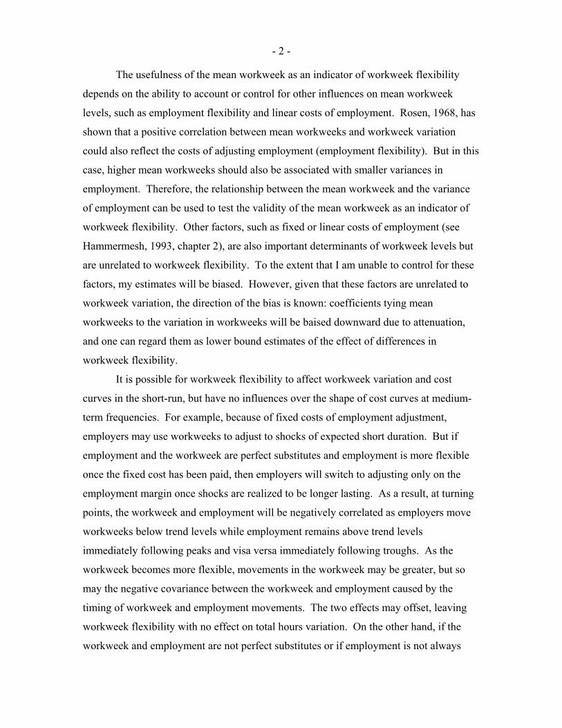
First, I show that across industry differences in workweek flexibility is significant

and that workweek flexibility is an important determinant of the cyclical variation in

workweeks, and, by implication, short-run cost curves. The intuition behind the

identification of the effect of workweek flexibility is shown in figure 1, where greater

flexibility in the form of flatter marginal product and/or marginal disutility curves for

hours per worker lead to a flatter workweek supply (marginal cost) curve for the flexible

industry (F) than for the inflexible industry (I). As a result, both the mean workweek and

the cyclical variation of the workweek (as produced by changes in a demand shifter, >,

and shown by the difference between H1 and H0) are greater in the flexible industry. To

test for differences in flexibility, I use the mean workweek as indicator of flexibility and

see whether industries with greater mean workweeks are also industries with greater

cyclical variances in workweeks.

- 2 -

The usefulness of the mean workweek as an indicator of workweek flexibility

depends on the ability to account or control for other influences on mean workweek

levels, such as employment flexibility and linear costs of employment. Rosen, 1968, has

shown that a positive correlation between mean workweeks and workweek variation

could also reflect the costs of adjusting employment (employment flexibility). But in this

case, higher mean workweeks should also be associated with smaller variances in

employment. Therefore, the relationship between the mean workweek and the variance

of employment can be used to test the validity of the mean workweek as an indicator of

workweek flexibility. Other factors, such as fixed or linear costs of employment (see

Hammermesh, 1993, chapter 2), are also important determinants of workweek levels but

are unrelated to workweek flexibility. To the extent that I am unable to control for these

factors, my estimates will be biased. However, given that these factors are unrelated to

workweek variation, the direction of the bias is known: coefficients tying mean

workweeks to the variation in workweeks will be baised downward due to attenuation,

and one can regard them as lower bound estimates of the effect of differences in

workweek flexibility.

It is possible for workweek flexibility to affect workweek variation and cost

curves in the short-run, but have no influences over the shape of cost curves at medium-

term frequencies. For example, because of fixed costs of employment adjustment,

employers may use workweeks to adjust to shocks of expected short duration. But if

employment and the workweek are perfect substitutes and employment is more flexible

once the fixed cost has been paid, then employers will switch to adjusting only on the

employment margin once shocks are realized to be longer lasting. As a result, at turning

points, the workweek and employment will be negatively correlated as employers move

workweeks below trend levels while employment remains above trend levels

immediately following peaks and visa versa immediately following troughs. As the

workweek becomes more flexible, movements in the workweek may be greater, but so

may the negative covariance between the workweek and employment caused by the

timing of workweek and employment movements. The two effects may offset, leaving

workweek flexibility with no effect on total hours variation. On the other hand, if the

workweek and employment are not perfect substitutes or if employment is not always

- 3 -

1. To the extent that overtime regulations influence marginal cost schedules, one would expectto find a negative relationship between mean workweeks and workweek flexibility, as higher

(continued...)

more flexible after the fixed cost has been paid, then greater workweek flexibility may

add to total hours variation.

In the former case, it is employment flexibility that determines the shape of

employers’ marginal cost schedules for shocks that are large enough or of long enough

duration. In the latter case, workweek flexibility is also an important determinant of the

shape of employers’ medium-term marginal cost curves, and greater flexibility should

lead to greater total hours variation over the cycle. The data support the latter

interpretation and imply that workweek flexibility affects medium-term cost curves as

well as short-run.

The relationship between flexibility and mean workweek levels raises the

possibility that the rise in the manufacturing workweek since the mid-1970s has been due

changes in factory production processes that have increased workweek flexibility. If this

were true, then the results from the cross sectional analysis described above should also

hold in a panel setting. More specifically, industries with large increases in mean

workweeks from 1972-1987 to 1987-1996 should also have experienced increases in the

relative variability of their workweeks. In fact, changes in mean workweeks appear to be

unrelated to changes in workweek variation. Therefore, I conclude that the rise in the

manufacturing workweek has likely owed to other factors, such as increases in workers’

skills, see Hetrick, 2000, or increases in employee benefits, see Beaulieu, 1995.

Most papers on the workweek have focused on the relationship between average

workweek levels and regulations on overtime compensation (Trejo, 2003, Hammermesh

and Trejo, 2000, and Costa, 2000) rather than the importance of the workweek as a

margin of hours adjustment. Bils, 1987, estimates the cost of increasing the workweek

but only considers costs related to overtime premiums. As Bernanke, 1986, shows, when

compensation schedules are non-linear, overtime premiums become irrelevant to the

choice of hours per worker, and the marginal cost of the workweek is determined instead

by the disutility of labor. I follow this approach, and in the model presented below

differences in workweek levels are not tied to compensation regulations.1 More closely

- 4 -

1. (...continued)workweeks push firms to a more inelastic portion of the workweek supply curve. In fact, asdescribed in section 5, I find a strong positive correlation.

2. Fleischman (1995) examines the effect of employment adjustment costs to across industryvariation in employment flexibility.

3. For more information about the survey, see Employment & Earnings, Bureau of LaborStatistics, Washington, D.C.

related to the current paper are Bernanke, 1986, who investigates the elasticity of hourly

earnings with respect to hours per worker for several industries during the Great

Depression, and Rosen, 1968, who uses average workweeks and cyclical variation in

workweeks as indirect measures of firm specific human capital. However, neither of

these papers, nor any other paper that I am aware of, has attempted to estimate the

importance of workweek flexibility to the variability of workweeks and aggregate hours

and, by implication, to firms’ marginal cost schedules.2

The next section describes the data on workweeks and employment. Section 3

constructs a simple model to illustrate how workweek flexibility is correlated with mean

workweek levels and variation in workweeks, employment and total hours. Section 4

uses the analysis in section 3 to construct estimation equations, section 5 presents results,

and section 6 concludes.

2. The data

Data on the workweek come from the Current Employment Statistics (CES)

survey. Each month the survey samples data from establishments representing about 30

percent of private nonfarm employment. For production workers, establishments are

asked for data on total hours paid and total employment for the pay period including the

12th of the month. The BLS converts the hours paid figure to a weekly basis and divides

by employment to compute average weekly hours.3

While aggregate employment data go back to 1939, detailed industry data on

workweeks is more limited. In addition, there are breaks in industry classification, the

most important occurring in 1972 and 1987. Consequently, I focus on two periods 1972-

1987 and 1988-1996. Each of these periods contains at least one recession, and during

each period industrial classification systems did not change. The 1972-1987 period

- 5 -

4. To preserve comparability across time I use disaggregated and aggregate data publishedprior to the conversion of the CES to NAICS and random sampling in June 2003, seeEmployment and Earnings, June 2003.

contains 151 four-digit industries representing 58 percent of manufacturing production

worker employment, while the 1988-1996 period contains 173 four-digit industries

representing 63 percent of manufacturing production worker employment. I also

construct a two period panel using those industries which were not affected by the break

in industry classification in 1987 (the large majority).

The CES also provides data on earnings and the number of women workers but

does not collect any output related data. For this I rely instead on annual data from the

NBER productivity database. The data on value added from this source extend through

1996 and determines the terminal point of my sample.

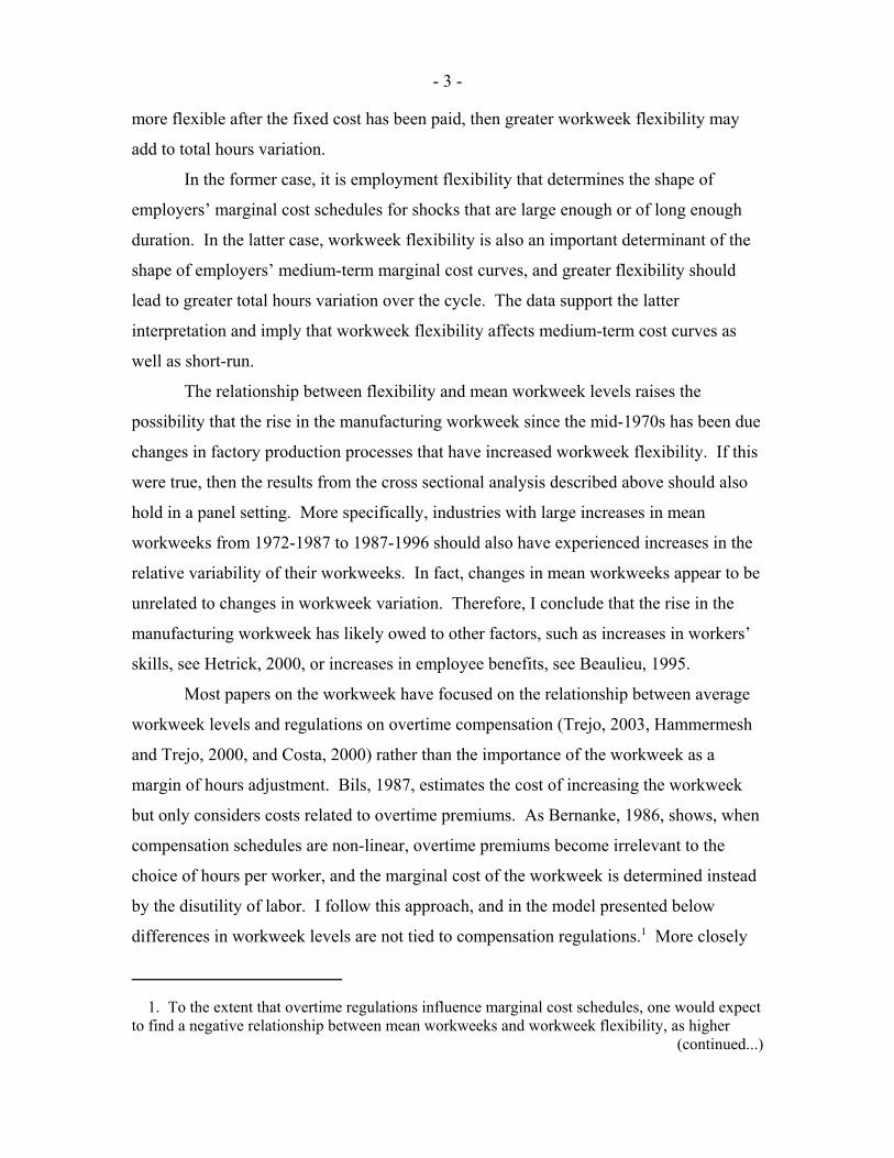
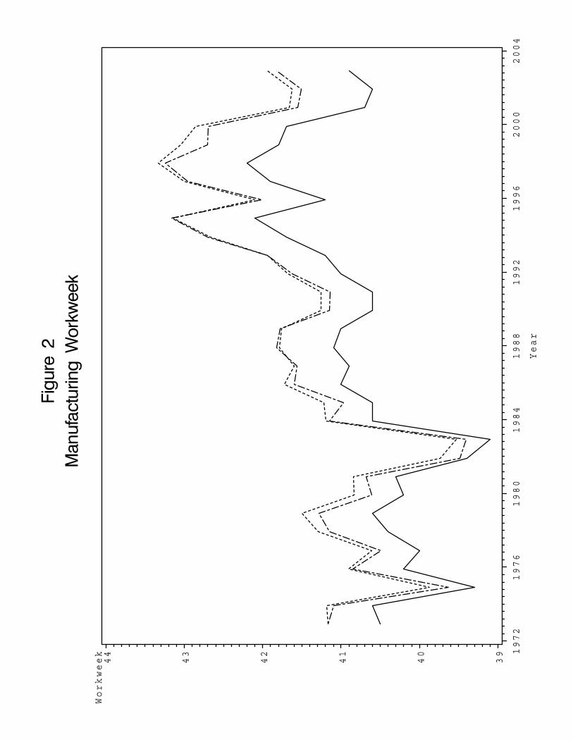
To get a sense of the representativeness of my sample, I compute a weighted

average of workweeks from sampled industries and compare the result with the published

data for the aggregate manufacturing sector.4 Observations are for the last month of the

relevant year. Figure 2 shows these time series. For the most part, the behavior of the

two measures is quite similar, though sample workweeks tend to be above the average for

the aggregate manufacturing sector. As shown in the figure, the mean workweek

increased significantly from the early 1970s to the late 1990s. The dot-dashed line in the

figure also shows what the increase in the workweek would have been had all

employment shares been held constant at their 1972 levels. It is apparent that industry

shifts were not an important contributor to the rise in the workweek over the thirty years

of the sample.

The workweek has important high and low frequency components to its total

variation. I am interested in the component of variation related to the business cycle and

use a band pass filter from Baxter and King, 1999, to remove both very high and very

low frequency variation. Specifically, I isolate the components of the workweek with a

period of between one and one-half and eight years. The Baxter-King filter uses a

symmetric backward and forward weighted moving average to isolate these frequencies.

Following their recommendation, I use a centered seven-year window to compute these

moving averages. This reduces the years used in my analysis to 1975-1984 and 1991-

- 6 -

5. Because use of the Baxter-King filter on value added data would limit my second periodsample to 1991-1993, I instead remove the trend in this second period by regressing value addedon a time trend.

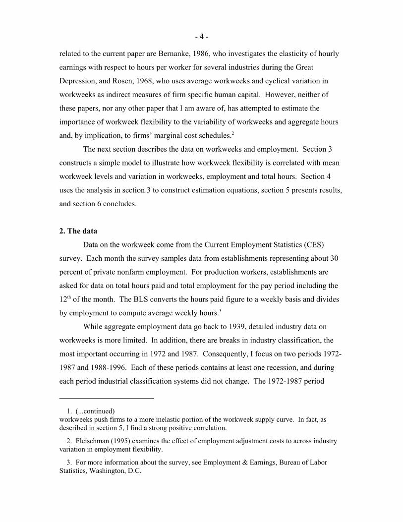
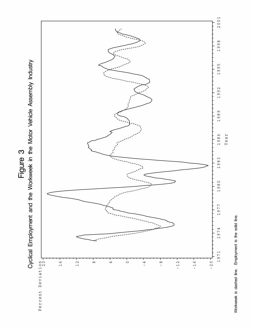
1996.5 I also isolate the cyclical components of production worker employment and

production worker hours. To focus on percent deviations from long term trends, I take

the natural log of variables before filtering. To illustrate the behavior of the resulting

variables, figure 3 plots the cyclical components of the workweek and employment for

the automobile assembly industry.

Table 1 shows statistics on the cross industry distribution of the variables I will be

using in my analysis: the across-industry means and standard deviations of the natural

log of hours per worker, average hourly earnings, and the share of women workers; and

the across industry means and standard deviations of the variances of the cyclical

components of the natural logs of hours per worker, production worker employment, total

production worker hours, and value added. The table shows that the average variance of

the percent deviation of production worker employment from its long-term trend is well

in excess of the same measure for the workweek, indicating that employment has been a

more important margin of hours adjustment. As shown by the second and fourth

columns in the table, there appears to be considerable across industry variation in both

average workweek levels and cyclical movements in the workweek and employment.

3. Model

I use a simple partial equilibrium model drawn largely from Bernanke, 1986, of a

profit maximizing firm choosing employment and hours per worker subject to a

participation constraint for workers. Workers derive utility from consumption and

leisure and are willing to work if the offered package of hours and compensation

provides them with utility at least equal to their best alternative. The model shows that

an employer’s reliance on the workweek to adjust hours in response to a shock to

marginal revenue will depend on the workweek’s flexibility. An input is more flexible

the smaller are the absolute values of the elasticities of the revenue and cost functions

with respect to the input.

- 7 -

6. The cost of employee training is one example of such a cost. However, to the extent thatsuch training is firm specific, it may (as Rosen, 1968) shows be positively correlated withemployment flexibility.

Input flexibilities are not observed, but the model shows that the mean workweek

should be positively correlated with workweek flexibility and thus can act as a proxy for

it. However, the mean workweek reflects factors other than workweek flexibility, and it

is important to control or account for their effects. The model shows that a positive

correlation between the mean and variance of workweeks could reflect the influence of

employment flexibility, rather than workweek flexibility. This is because industries with

less flexible employment should have more variable workweeks and perhaps higher

mean workweeks. However, in this case, mean workweeks should be negatively

correlated with employment variation. Thus, the relationship between workweek

flexibility and employment variation can be used to test whether the relationship between

the mean and variance of workweeks is due to workweek flexibility rather than

employment flexibility. In addition, there exist factors that influence mean workweek

levels without changing either employment or workweek flexibility (e.g. fixed costs of

employment or costs that vary linearly with employment).6 To the extent that such

factors cannot be controlled for using observable variables, they render the workweek an

imperfect gauge of workweek flexibility and biased downward coefficients estimating

the effect of workweek flexibility on workweek variation.

Though workweek flexibility may be relevant for firms’ cost curves over the

short-run, as time horizons lengthen, or as shocks are recognized as more permanent,

employers may substitute employment adjustment for the workweek. To illustrate this, I

modify the model to allow for sunk costs of employment adjustment. In such a model,

workweek flexibility may flatten firms’ cost curves when shocks are small enough or of

short enough expected duration to limit hours adjustment to movements in the workweek.

Over longer time horizons, however, firms may rely solely on employment to adjust

hours. In this case, the relationship between workweek flexibility and total hours

variation may be quite weak, with the implication that greater workweek flexibility may

not change the shape of cost curves relevant for medium term movements in demand. A

- 8 -

significant relationship between workweek flexibility and total hours variation would,

however, lead one to the opposite conclusion.

The object of the analysis below is not to construct structural models of hours

demand and hours supply to then take to the data. The assumptions required to be able to

use my data to identify relevant parameters would likely render estimated coefficients

relatively meaningless. Instead, I assume that fluctuations in hours at cyclical

frequencies are due entirely to labor demand shocks. Measures of variability of labor

inputs thus provide information about the shape of labor supply curves, or firm’s short-

run cost curves. Rather than parameterize these curves, I, instead, examine the

relationship between labor input variability and a measure of workweek flexibility (mean

workweeks) to see if workweek flexibility is an important determinant of across industry

differences in short-run and medium-run cost curves.

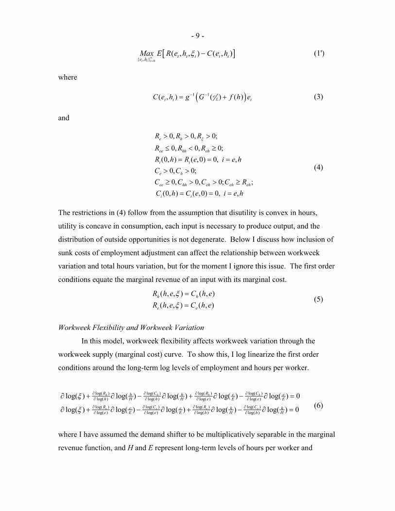
In the model an employer chooses employment, compensation per worker and

weekly hours per worker to maximize profits subject to a participation constraint.

(1)0{ , , } 0

*

( , , )

. . ( , ) 0t t t t

tt t t t t

e h W t

Max E R e h eW

s t U W h U

β ξ∞= =

− − ≥

∑

where $ is a discount factor, R is revenue, e is employment, h is hours per worker, W is

compensation per worker, > is a marginal revenue shifter, U* is the utility value of a

worker’s next best alternative, and E is the expectations operator. I assume that U is

additively separable in its two arguments and that workers’ outside opportunities are

distributed according to the cumulative density function, .*( )G U

(2)* 1

( , ) ( ) ( )( ) 0, ( ) 0; ( ) 0, 0

( )eL

U c h g c f hg c g c f h fc WU G−

= −′ ′′ ′ ′′> < > >=

=

where c is consumption and L is the exogenous total labor supply available to the firm.

One can then substitute out W using the participation constraint and the fact that

consumption is equal to compensation (there is no saving in the model) to get

- 9 -

(1')[ ]0{ , }

( , , ) ( , )t t t

t t t t te hMax E R e h C e hξ

∞=

−

where

(3)( )1 1( , ) ( ) ( )eLt t tC e h g G f h e− −= +

and

(4)

0, 0, 0;

0, 0, 0;(0, ) ( ,0) 0, ,

0, 0;0, 0, 0; ;

(0, ) ( ,0) 0, ,

e h

ee hh eh

i i

e h

ee hh eh eh eh

i i

R R R

R R RR h R e i e hC CC C C C RC h C e i e h

ξ> > >

≤ < ≥= = =

> >≥ > > ≥

= = =

The restrictions in (4) follow from the assumption that disutility is convex in hours,

utility is concave in consumption, each input is necessary to produce output, and the

distribution of outside opportunities is not degenerate. Below I discuss how inclusion of

sunk costs of employment adjustment can affect the relationship between workweek

variation and total hours variation, but for the moment I ignore this issue. The first order

conditions equate the marginal revenue of an input with its marginal cost.

(5)( , , ) ( , )( , , ) ( , )

h h

e e

R h e C h eR h e C h e

ξξ

==

Workweek Flexibility and Workweek Variation

In this model, workweek flexibility affects workweek variation through the

workweek supply (marginal cost) curve. To show this, I log linearize the first order

conditions around the long-term log levels of employment and hours per worker.

(6)

log( ) log( ) log( ) log( )log( ) log( ) log( ) log( )

log( ) log( ) log( ) log( )log( ) log( ) log( ) log( )

log( ) log( ) log( ) log( ) log( ) 0

log( ) log( ) log( ) log( )

h h h h

e e e e

R C R Ch h e eh H h H e E e E

R C R Ce e he E e E h H h

ξ

ξ

∂ ∂ ∂ ∂∂ ∂ ∂ ∂

∂ ∂ ∂ ∂∂ ∂ ∂ ∂

∂ + ∂ − ∂ + ∂ − ∂ =

∂ + ∂ − ∂ + ∂ − log( ) 0hH∂ =

where I have assumed the demand shifter to be multiplicatively separable in the marginal

revenue function, and H and E represent long-term levels of hours per worker and

- 10 -

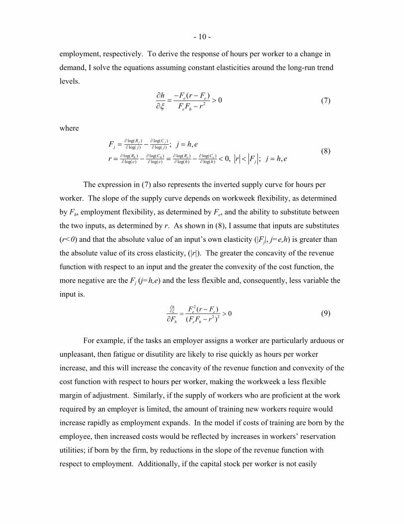
employment, respectively. To derive the response of hours per worker to a change in

demand, I solve the equations assuming constant elasticities around the long-run trend

levels.

(7)2

( ) 0e e

e h

h F r FF F rξ

∂ − −= >

∂ −

where

(8)log( ) log( )log( ) log( )

log( ) log( ) log( ) log( )log( ) log( ) log( ) log( )

; ,

0, ; ,

j j

h h e e

R Cj j j

R C R Cje e h h

F j h e

r r F j h e

∂ ∂∂ ∂

∂ ∂ ∂ ∂∂ ∂ ∂ ∂

= − =

= − = − < < =

The expression in (7) also represents the inverted supply curve for hours per

worker. The slope of the supply curve depends on workweek flexibility, as determined

by Fh, employment flexibility, as determined by Fe, and the ability to substitute between

the two inputs, as determined by r. As shown in (8), I assume that inputs are substitutes

(r<0) and that the absolute value of an input’s own elasticity (|Fj|, j=e,h) is greater than

the absolute value of its cross elasticity, (|r|). The greater the concavity of the revenue

function with respect to an input and the greater the convexity of the cost function, the

more negative are the Fj (j=h,e) and the less flexible and, consequently, less variable the

input is.

(9)2

2 2

( ) 0( )

he e

h e h

F r FF F F rξ∂∂ −

= >∂ −

For example, if the tasks an employer assigns a worker are particularly arduous or

unpleasant, then fatigue or disutility are likely to rise quickly as hours per worker

increase, and this will increase the concavity of the revenue function and convexity of the

cost function with respect to hours per worker, making the workweek a less flexible

margin of adjustment. Similarly, if the supply of workers who are proficient at the work

required by an employer is limited, the amount of training new workers require would

increase rapidly as employment expands. In the model if costs of training are born by the

employee, then increased costs would be reflected by increases in workers’ reservation

utilities; if born by the firm, by reductions in the slope of the revenue function with

respect to employment. Additionally, if the capital stock per worker is not easily

- 11 -

expanded, then the marginal product of workers may decrease as workers are added. In

these circumstances, employment would not be a very flexible factor. Finally, variation

in an input depends on the other input’s flexibility and the elasticity of substitution

between the two inputs. If the other input is relatively more flexible and it is fairly easy

to substitute one input for another, then an input’s variation will decline.

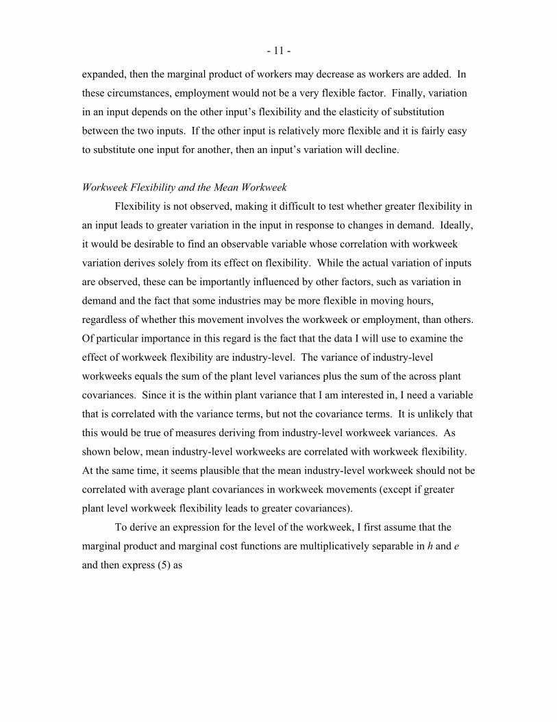
Workweek Flexibility and the Mean Workweek

Flexibility is not observed, making it difficult to test whether greater flexibility in

an input leads to greater variation in the input in response to changes in demand. Ideally,

it would be desirable to find an observable variable whose correlation with workweek

variation derives solely from its effect on flexibility. While the actual variation of inputs

are observed, these can be importantly influenced by other factors, such as variation in

demand and the fact that some industries may be more flexible in moving hours,

regardless of whether this movement involves the workweek or employment, than others.

Of particular importance in this regard is the fact that the data I will use to examine the

effect of workweek flexibility are industry-level. The variance of industry-level

workweeks equals the sum of the plant level variances plus the sum of the across plant

covariances. Since it is the within plant variance that I am interested in, I need a variable

that is correlated with the variance terms, but not the covariance terms. It is unlikely that

this would be true of measures deriving from industry-level workweek variances. As

shown below, mean industry-level workweeks are correlated with workweek flexibility.

At the same time, it seems plausible that the mean industry-level workweek should not be

correlated with average plant covariances in workweek movements (except if greater

plant level workweek flexibility leads to greater covariances).

To derive an expression for the level of the workweek, I first assume that the

marginal product and marginal cost functions are multiplicatively separable in h and e

and then express (5) as

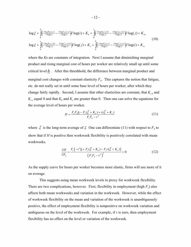
- 12 -

(10)( ) ( )

( ) ( )

log ( , ) log ( , ) log ( , ) log ( , )log( ) log( ) log( ) log( )

0 0

log ( , ) log ( , ) log ( , ) log ( , )log( ) log( ) log( ) log( )

0

log log( ) log( )

log log( )

h h h h

e e e e

h eR e i C e i R j h C j h

h rhi i j j

eR j h C j h R e i C e i

ej j i i

i K j K

j K

ξ

ξ

∂ ∂ ∂ ∂∂ ∂ ∂ ∂

∂ ∂ ∂ ∂∂ ∂ ∂ ∂

+ − ∂ + + − ∂ +

+ − ∂ + + −

∫ ∫

∫0

log( )h

rei K∂ +∫

where the Ks are constants of integration. Next I assume that diminishing marginal

product and rising marginal cost of hours per worker are relatively small up until some

critical level . After this threshhold, the difference between marginal product andh

marginal cost changes with constant elasticity Fh. This captures the notion that fatigue,

etc. do not really set in until some base level of hours per worker, after which they

change fairly rapidly. Second, I assume that other elasticities are constant, that Kr,h and

Kr,e equal 0 and that Kh and Ke are greater than 0. Then one can solve the equations for

the average level of hours per worker.

(11)2

( ) ( )e h e h e

e h

F F h F K r KHF F rξ ξ− + + +

=−

where is the long-term average of >. One can differentiate (11) with respect to Fh toξ

show that if H is positive then workweek flexibility is positively correlated with mean

workweeks.

(12)( )( )

2

22

( ) ( )0e e h e e

h e h

F r h F K F r KHF F F r

ξ ξ− + + − +∂= >

∂ −

As the supply curve for hours per worker becomes more elastic, firms will use more of it

on average.

This suggests using mean workweek levels to proxy for workweek flexibility.

There are two complications, however. First, flexibility in employment (high Fe) also

affects both mean workweeks and variation in the workweek. However, while the effect

of workweek flexibility on the mean and variation of the workweek is unambiguously

positive, the effect of employment flexibility is nonpositive on workweek variation and

ambiguous on the level of the workweek. For example, if r is zero, then employment

flexibility has no effect on the level or variation of the workweek.

- 13 -

7. In Rosen, 1968, employment flexibility and linear costs of employment (hiring costs) arecorrelated because of firm-specific capital. In this case, one would expect the mean and varianceof the workweek to be positively correlated, but one would also expect a negative correlationbetween the mean workweek and employment variation. In addition, to the extent that theelasticities of marginal product and marginal cost increase as h increases, one would expectincreases in Ke to lead to decreases in workweek variation and offset the positive correlationbetween the mean and variance of the workweek mentioned above.

In addition, the employment supply curve depends positively on employment

flexibility

(13)2 2

( ) 0( ) ( )

eh h

e e h

r F FF F F rξ∂∂∂ − −

= >∂ −

Thus, one can check the validity of the assumption that any positive correlation between

the mean and variance of workweeks reflects workweek flexibility rather than

employment flexibility by seeing whether mean workweek levels are negatively

correlated with employment variation.

A second complication is that other factors, such as fixed costs of employment

(see Hammermesh, 1993, chapter 2), which would be captured in Ke, are also important

in determining workweek levels. However, as shown in equation (7), they have no effect

on workweek variation. Thus, to the extent that they are not controlled for, the mean

workweek will be a noisy measure of workweek flexibility, and estimates of the effect of

workweek flexibility on workweek variation will be biased downward due to

attenuation.7

Total Hours Variation and Workweek Flexibility

In the model described above workweek flexibility adds both to workweek

variation and total hours variation. The variance of the log of total hours is

(14)(log( * )) (log( )) (log( )) 2 * (log( ), log( ))var e h var h var e Cov h e= + +

One can show that

(15)

(log( )) (log( ))0, 0,( ) ( )

(log( )) (log( )) , (log( ), log( )) 0( )

h h

h h

Var h Var eF F

Var h Var e Cov h eF F

∂ ∂> <

∂ ∂

∂ ∂> >

∂ ∂

- 14 -

8. For more on the dynamic behavior of the workweek, see Golden (1990) and Glosser andGolden (1990).

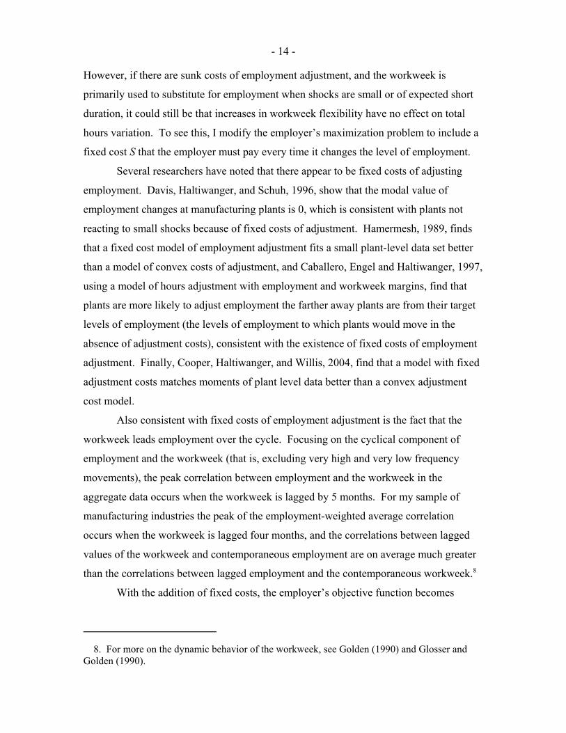
However, if there are sunk costs of employment adjustment, and the workweek is

primarily used to substitute for employment when shocks are small or of expected short

duration, it could still be that increases in workweek flexibility have no effect on total

hours variation. To see this, I modify the employer’s maximization problem to include a

fixed cost S that the employer must pay every time it changes the level of employment.

Several researchers have noted that there appear to be fixed costs of adjusting

employment. Davis, Haltiwanger, and Schuh, 1996, show that the modal value of

employment changes at manufacturing plants is 0, which is consistent with plants not

reacting to small shocks because of fixed costs of adjustment. Hamermesh, 1989, finds

that a fixed cost model of employment adjustment fits a small plant-level data set better

than a model of convex costs of adjustment, and Caballero, Engel and Haltiwanger, 1997,

using a model of hours adjustment with employment and workweek margins, find that

plants are more likely to adjust employment the farther away plants are from their target

levels of employment (the levels of employment to which plants would move in the

absence of adjustment costs), consistent with the existence of fixed costs of employment

adjustment. Finally, Cooper, Haltiwanger, and Willis, 2004, find that a model with fixed

adjustment costs matches moments of plant level data better than a convex adjustment

cost model.

Also consistent with fixed costs of employment adjustment is the fact that the

workweek leads employment over the cycle. Focusing on the cyclical component of

employment and the workweek (that is, excluding very high and very low frequency

movements), the peak correlation between employment and the workweek in the

aggregate data occurs when the workweek is lagged by 5 months. For my sample of

manufacturing industries the peak of the employment-weighted average correlation

occurs when the workweek is lagged four months, and the correlations between lagged

values of the workweek and contemporaneous employment are on average much greater

than the correlations between lagged employment and the contemporaneous workweek.8

With the addition of fixed costs, the employer’s objective function becomes

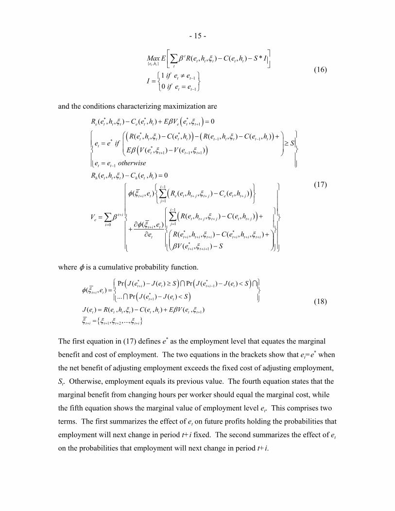
- 15 -

(16){ , }

1

1

( , , ) ( , ) *

10

t t

tt t t t te h t

t t

t t

Max E R e h C e h S I

if e eI

if e e

β ξ

−

−

− − ≠

= =

∑

and the conditions characterizing maximization are

(17)

( )( ) ( )

( )

* * *1

* *1 1*

*1 1 1

1

( , , ) ( , ) , 0

( , , ) ( , ) ( , , ) ( , )

( , ) ( , )

( , , ) ( , ) 0

( ,

e t t t e t t e t t

t t t t t t t t t t

t

t t t t

t t

h t t t h t t

t i t

t ie

R e h C e h E V e

R e h C e h R e h C e he e if S

E V e V e

e e otherwise

R e h C e h

e

V

ξ β ξ

ξ ξ

β ξ ξ

ξ

φ ξ

β

+

− −

+ − +

−

+

+

− + =

− − − + = ≥ −

= − =

=

( )

( )

1

1

1

10

* *

*1

) ( , , ) ( , )

( , , ) ( , )( , )

( , , ) ( , , )

( , )

i

e t t j t j e t t jj

i

t t j t j t t jji t i t

t i t i t i t i t i t it

t i t i

R e h C e h

R e h C e he

R e h C e heV e S

ξ

ξφ ξ

ξ ξ

β ξ

−

+ + +=

−

+ + +== +

+ + + + + +

+ + +

−

− +

∂ + − +∂ −

∑

∑∑

where N is a cumulative probability function.

(18)

( ) ( )( )

{ }

* *1

*1

1

1 2

Pr ( ) ( ) Pr ( ) ( )( , )

... Pr ( ) ( )

( ) ( , , ) ( , ) ( , ), ,...,

t i t t i t

t i t

t t

t t t t t t t t

t i t t t i

J e J e S J e J e Se

J e J e S

J e R e h C e h E V e

φ ξ

ξ β ξ

ξ ξ ξ ξ

+ + −

+

+

+

+ + + +

− ≥ − < = − <

= − +

=

I I

I

The first equation in (17) defines e* as the employment level that equates the marginal

benefit and cost of employment. The two equations in the brackets show that et=e* when

the net benefit of adjusting employment exceeds the fixed cost of adjusting employment,

St. Otherwise, employment equals its previous value. The fourth equation states that the

marginal benefit from changing hours per worker should equal the marginal cost, while

the fifth equation shows the marginal value of employment level et. This comprises two

terms. The first summarizes the effect of et on future profits holding the probabilities that

employment will next change in period t+i fixed. The second summarizes the effect of et

on the probabilities that employment will next change in period t+i.

- 16 -

From these conditions follow several observations about the dynamics of

employment and the workweek. First, employment will not adjust to all shifts in

demand. Specifically, if the net benefit of adjusting employment is less than the fixed

cost, S, employment will not adjust. Second, since there are no costs of adjusting the

workweek, the workweek will adjust to all changes in > when there is no employment

adjustment, though, perhaps not to changes in > when there is employment adjustment.

These observations are consistent with the facts noted above that employment at the plant

level appears not to adjust to all shocks and that the manufacturing workweek leads

employment over the business cycle. Third, an increase in the expected duration of a

shock increases adjustment along the employment margin and decreases adjustment

along the workweek margin. This can be seen by substituting the last equation from (17)

into the first. The value of adjusting employment depends negatively on the likelihood of

having to adjust employment back toward its t-1 value in period t+1. Thus, when faced

with shocks of expected short duration, employers will rely more heavily on the

workweek margin.

To see how the inclusion of fixed costs affects the relationship between

workweek flexibility and total hours variation, suppose there are two types of shocks, a

transitory shock and a lasting shock, that there are two states, and , that the revenueξ ξ

and cost function are homogeneous of degree one in employment, and that the

distribution of U* (threshold utility) is degenerate. Suppose also that initially an

employer is uncertain about whether the shock is transitory or lasting, but that after one

period the persistence of the shock is known. If the initial probability that it is a long-

duration shock is small enough, the employer will change the workweek, but not

employment. And, if the workweek is more flexible, the employer will change the

workweek by more. However, if the size of the shock is large enough, then once the

shock is deemed to be permanent, the employer will adjust employment and move hours

per worker back to its original value. In this case, a more flexible workweek allows an

employer to adjust hours by more sooner, but in the end the change in hours from its peak

to its trough is not affected. This is because, given a large enough shock with long

enough duration, employment is infinitely flexible (revenue and cost functions are

homogeneous of degree 1 in employment) in the long run and, thus, employers will

- 17 -

9. I estimate trends using a low pass filter. Using mean trends controls for circumstances inwhich the cyclical conditions for an industry do not average to be neutral over the time period inquestion.

adjust only along this margin. Given both the duration and magnitude of cyclical

fluctuations, the influence of workweek flexibility on cyclical total hours variation may

be minimal.

4. Estimation Equations

Workweek variation (Short-run Cost Curves)

The above analysis suggests using the average workweek as an observable

variable to proxy for the flexibility of the workweek in the following estimation

equations.

(19)1 1,1 1

2,1 1 2 2,2 2

3,1 1 3 3,2 3

var

var

i i iww

i i i ie

i i i iww

X

X

X

µ β ε

β ε β ε

β ε β ε

= +

= + +

= + +

where i indexes industry, :ww represents the mean of the natural log of the trend

workweek, vare represents the variance of detrended log employment, and varww

represents the variance of the detrended log workweek.9

In the first equation, X1 contains variables correlated with factors, such as high

fixed costs of employment (Ke is high), that affect the average level of the workweek but

are not related to workweek flexibility. The residual from this regression should then be

purged of some of the variation unrelated to flexibility. If the variables in X1 fail to fully

control for these other factors, then the residual will contain their effect as well, and it

will be an imperfect proxy for workweek flexibility. Given that the factors affecting only

first derivatives of the profit function (Ke, Kh ) have no effect on workweek variation,

their inclusion in g1 will bias toward zero coefficients estimating the effect of workweek

flexibility on employment variation and workweek variation in the next two equations.

In the second equation, the coefficient on g1 should be less than or equal to zero

(higher workweek flexibility should have a nonpositive effect on employment variation).

X2 in this equation contains observable variables correlated with the cyclical variance of

employment, such as an industry’s demand variability. There also likely exist factors

- 18 -

that cause both the workweek and employment to be more flexible and that are distinct

from workweek flexibility, which describes the ease of adjusting the workweek

independent of the ease of adjusting employment. For example, if a plant has a certain

minimum number of hours each week that must be devoted to plant maintenance (where

these hours can come from either employment or hours per worker), then its ability to

adjust hours downward would be constrained. If not correlated with observables, such

factors should be captured in the residual of the second equation.

The third equation then relates variation in the workweek to workweek flexibility

(as proxied by g1) and observable variables correlated with important determinants of

workweek variation, such as demand variability and the flexibility in total hours.

Identification of the effect of workweek flexibility rests on the assumption that the

correlation between the variance and mean of workweeks reflects workweek flexibility

rather than employment flexibility. The second and third equations in (19) provide a

simple test of this assumption. If the correlation reflects employment flexibility, then the

coefficient on the mean workweek in the second equation flexibility should be negative.

Total Hours Variation (Medium-term Cost Curves)

Equation (14) and the analysis of workweek flexibility and hours variation in

section 3 suggest testing for the influence of workweek flexibility on medium term cost

curves with the following equation

(20), ,4,1 4,2 4,3 3 4 4var( ) var( ) var( ) var( )i i f i o i i iTH ww ww eβ β β ε β ε= + + + +

in which total hours variation is regressed on components of workweek variation and

employment variation. The first component of workweek variation, vari,f(log(ww)),

represents the contribution of workweek flexibility to workweek variation and is the

product of g1 and its estimated coefficient from the third equation of (19). The second

and third components represent the effects of observed and unobserved variables,

respectively, on workweek variation. The second component is computed as the

predicted value from the third equation in (19) minus the effect attributable to workweek

flexibility, while the third component is the residual from the third equation in (19).

- 19 -

The error term in this equation, , contains the covariance between employment4iε

and the workweek. Thus, the estimate of $4,1 will contain both the direct effect of

workweek flexibility on total hours variation and the indirect effect due to any tendency

for increased workweek variation caused by greater workweek flexibility to be negatively

correlated with the covariance between employment and the workweek, as discussed in

section 3. Estimates of $4,1 significantly different from 0 would indicate that the direct

effect outweighs the indirect effect and that workweek flexibility flattens medium term as

well as short-term cost curves.

5. Results

Table 2A shows results from the estimation of the third equation in (19). The

first four columns display results for the 1972-1987 period, the next four for the 1988-

1996 period. Within each sample period, the four columns display results under different

assumptions regarding the variables contained in X1, X2, and X3. Because there is no

direct correspondence between the observable variables at hand and the theoretically

relevant variables and/or parameters and because the indirect correspondence seems

stronger for some observed variables than others, it seems reasonable to see how robust

results are to different specifications. Because observations for some variables were not

always available, the sample size reported in the last row of table 2A varies across

specification. All regressions are OLS, and observations are weighted by industries’

number of production workers.

In columns headed by (1) in table 2A, I report results from a bare-bones

specification including only a constant and the variance of the cyclical component of the

log of value added (to capture the effects of differences in demand variation) in X2 and X3

and only a constant in X1. The second specification, results of which are reported in

columns headed by (2), is similar to the first, only it excludes the cyclical variation in

value added from the workweek variation equation to see whether the endogeneity of this

variable is important (greater workweek flexibility should cause greater variation in value

added).

In the third specification, results of which are reported in columns headed by (3),

I use variables that appear to have a reasonably direct correspondence to variables and/or

- 20 -

10. Oi, 1962, and Rosen, 1968, argue that workers with greater specific human capital shouldhave smaller employment variation, which might indicate that average hourly earnings should benegatively correlated with employment variation and, thus, should be included in X2. However,empirically average hourly earnings are significantly positively correlated with employmentvariability. It must be that average hourly earnings are correlated with some unobservablevariable (unionization, the prevalence of temporary layoffs) that increases employment variation. Not knowing the source of its correlation with employment variation, I leave average hourlyearnings out of X2 in the third specification, including its effect, instead, in the residual of thesecond equation of (19). In the fourth specification, average hourly earnings are included as aright hand side variable in the second equation of (19).

parameters that likely enter the relevant equation. For X1 I use the percent of women

workers and average hourly earnings. Because of child-rearing responsibilities, women

may be drawn to industries with relatively low fixed costs of employment ( is low)ieK

and hence relatively low workweeks. Regarding average hourly earnings, Rosen, 1968,

argues that because of firm specific skills, high wages and high workweeks should be

positively correlated. The usefulness of average hourly earnings in capturing this effect

will depend on the share of across industry variation in average hourly earnings due to

firm-specific human capital and the share of across industry variation due to other

factors, such as general human capital. In X2 I include the cyclical variance of the log of

value added and a dummy variable for continuous processors.10 The latter variable may

partially control for variation in the flexibility of total hours. Continuous processors have

workweeks of capital close to the maximum when operating (e.g. chemical plants, paper

mills, petroleum refineries), see Mattey and Strongin, 1994, and thus may have higher

minimum required hours than other industries. For X3, I use the cyclical variance of

value added, a dummy variable for continuous processors and (which may capture2ε

the effect of greater total hours flexibility—to the extent it is not captured by the

continuous processor dummy—as well as other determinants of production worker

variability not included in X2).

In the fourth specification, I include the share of women workers, average hourly

earnings, a continuous processor dummy, and the cyclical variances of value added and

production worker employment in X3 and all of these variables except the cyclical

variance of production worker employment in X2. If there is a poor correspondence

between the observable variables chosen for the third specification and the theoretically

- 21 -

relevant variables and/or parameters, then estimation results from the third specification

may stem from spurious correlations. In this case, it may be better to control for all

observable variables. Table 3 shows the variables used in each equation under the four

different specifications.

The main results in table 2A are that workweek flexibility varies significantly

across industries and that greater flexibility leads to greater workweek variation and,

implicitly, flatter short-run marginal cost curves. In the 1972-87 period, most estimates of

$3,1 are near 2, which means that a two hour, or 5 percent, increase in the workweek leads

to an increase in the variance of the percent deviation of the workweek from its long-term

trend of about 0.1, or about a third of a standard deviation of the variance. The

interpretation of these estimates is that the short-run marginal cost curve is flatter in

industries with more flexible workweeks, though the estimated effect of workweek

flexibility is not large. However, it is important to note that the estimated effect is likely

a lower bound. As discussed in sections 3 and 4, my controls for fixed employment costs

(contained in Ke) may not be adequate and, as a result, my proxy for workweek flexibility

may contain substantial measurement error, producing attenuation bias. Given both the

limited number of controls and the fairly rough correspondence between them and the

characteristics (e.g. linear costs of employment, firm specific human capital) that theory

suggests should matter, this is almost certainly the case.

The estimates of $3,2 and $3,3 for the 1972-1987 period are as expected. The

variance of value added significantly increases workweek variation and the residual from

the second equation in (19) has a significantly positive coefficient, implying that it

captures the effect of greater total hours flexibility.

Table 2B shows estimates for the second equation of (19) for the 1972-1987

period. These support the assumption that the positive association between the mean and

variance of workweeks found from estimating the third equation of (19) reflects

workweek rather than employment flexibility. The coefficient on the mean workweek is

estimated to be positive but not significantly different from 0 in all specifications. The

- 22 -

11. Estimation results from the first equation of (19) for the third specification (not shown)were as expected: the share of women workers significantly lowers the mean workweek, and thelevel of average hourly earnings raises it.

12. If employment and the workweek are substitutes, less employment flexibility should leadto greater workweek variation. If, however, the reduction in employment flexibility moves firmsup an increasingly inelastic workweek supply curve, then the negative association betweenemployment flexibility and workweek variation could be offset or even reversed.

other coefficient estimates for the second equation are as expected: the variance of value

added adds to employment variance, while the continuous process dummy decreases it.11

Estimated coefficients from the 1988-96 period are different from the earlier

period, perhaps because labor market conditions were also different. The recession

during this period was shallower than the recessions in the earlier period, and the

downturn in the labor market was more drawn out. Other changes in manufacturing

labor markets, such as the increasing use of temporary help workers, also took place in

this period. The mean workweek during this period does not appear to have been as good

an indicator of workweek flexibility as in the earlier period, particularly that portion of

the workweek orthogonal to other observable variables. Part of the explanation for this

appears to be that employment flexibility became a more important determinant of mean

workweeks during this period.

In the 1988-1996 period, estimates of $3,1 from the third and fourth specifications,

which use variation in the workweek orthogonal to other observable variables to identify

the effect of workweek flexibility, are not statistically different from 0, and estimates of

$2,1 are significantly less than 0. These results are consistent with the variation in mean

workweeks across industries being due to employment flexibility rather than workweek

flexibility.12 Estimates of $3,1 in the first two specifications, which use the variation in

the workweek that is both orthogonal and correlated with other observable variables to

identify the effect of workweek flexibility, are, on average, below estimates from the

earlier period, though they are still significantly positive. Overall, the smaller estimated

$3,1s for this time period do not appear to owe to a smaller influence of workweek

flexibility on across industry differences in cost curves. Rather they appear to be due to a

weaker correlation between mean workweeks and workweek flexibility.

- 23 -

13. Biased coefficient estimates for the third equation in (19) could also be responsible for themagnitude of estimates of $4,1. While measurement error in my proxy for workweek flexibilitywould bias coefficient estimates of $4,1 downward, downward biased estimates of $3,1 would biasestimates of $4,1 upward. The net effect is uncertain, but perhaps the latter effect dominates. Inthis case, accounting for upward bias would diminish the magnitude of the estimated effect ofworkweek flexibility on total hours variation; it would not, however, change the sign.

Turning to the effect of workweek flexibility on total hours variation, table 4

shows estimates from equation (20). As shown in the first row, for the 1972-1987 period

the coefficient on workweek variation due to workweek flexibility is significantly

different from 0 in all specifications, with an average estimate close to 5. One

explanation for these results is that employment and the workweek covary negatively

over the cycle in industries with low workweek flexibility, but, as the workweek becomes

more flexible, firms cease using employment to substitute for it after sunk costs of

employment adjustment are paid, and the workweek and employment covary positively.

However, it is likely, given the large estimate, that across plant, as well as within plant

covariances are also at work.

As workweek flexibility increases, the covariance between employment and the

workweek across plants likely increases as well. Suppose that instead of a representative

agent model of the industry, in which flexibility is perfectly correlated across plants, that

plants in an industry have different levels of workweek flexibility, and that variation in

flexibility across industries reflects the number of plants within an industry that have

workweeks flexible enough to covary positively with employment. An industry with a

higher mean workweek has a greater number of plants whose workweeks covary

positively with employment. This also means that within these industries, the covariance

of employment and the workweek across plants will be greater—there will be more

plants of type i and j, for which when plant i’s workweek is below average, plant j’s

employment is below average and visa versa. Thus, the estimates in table 4 likely reflect

across plants, as well as within plant effects. Both effects are important. For questions

related to plant-level costs curves, one would only want the within plant effect, while for

industry-level cost curves, one would want both. Exactly what portion of the coefficient

estimate is due to within plant and what portion is due to across plant effects is not

possible to determine without plant-level data.13

- 24 -

For the 1988-1996 period, estimates from the first two specifications are both

positive, but both are less than one and neither is statistically significant. The limited

number of years in this period may make estimates less reliable, while the period’s

relatively mild, but drawn out, labor market downturn may cause estimates to differ from

those of the pervious period. The influence of employment flexibility on mean

workweeks during this period, described above, may also make it more difficult to

estimate the true effect of workweek flexibility.

As shown in figure 2, average workweeks have trended up over the past twenty-

five years. Thus, it could be that workweek flexibility increased over this period, which

would have potentially important implications for short-run and, perhaps, medium-run

cost curves. Although the change in the aggregate workweek seems to have been

reflected by increases in most industries, table 1 shows that there is still some variation in

the change in workweeks across industries. One should be aware, however, that the

source of variation in the change in average workweeks in the panel analysis may be

quite different from that in the cross sectional analysis and, thus, may not be closely tied

to workweek flexibility.

The last four columns of table 2A and 2B present estimates of the second two

equations in (19) after both sides of these equations have been differenced to reflect

changes from the 1972-87 period to the 1988-96 period. The main result, shown in table

2A, is that estimates for $3,1 are negative and not statistically significantly different from

zero. In addition, increases in mean workweeks have been associated with decreases in

employment variation, the second row of table 2B, though most estimates are not

significant. Thus, unless changes in workweek flexibility were constant across

industries, it is unlikely that increases in workweek flexibility were behind the increase in

the workweek over the past 25 years. Why the workweek has increased is uncertain.

Hetrick, 2000, suggests that manufacturing firms’ increased reliance on more skilled

workers may have lead to an increase in the workweek. Unions placing greater emphasis

on job security could also have been a factor. In addition, it could be that other factors,

not related to employment flexibility, such as a greater share of benefits in employee

compensation, may have caused the workweek to increase, see Beaulieu, 1995.

- 25 -

6. Conclusion

The reaction of producers to economic shocks depends on the how costly it is to

change inputs. This cost depends, in part, on the ease of varying workweeks, or on the

slopes of the workweek’s marginal product and marginal disutility curves—what I term

workweek flexibility. The organization of production process, which determines these

slopes, may differ across industries and may evolve over time, and this paper investigated

these possibilities. First, the paper demonstrated the relevance of workweek flexibility

by showing that it is a significant determinant of the cyclical variability of industry

workweeks and, by implications short-run marginal cost curves. Next, the paper

demonstrated that since employment is apparently not a perfect substitute for the

workweek over the business cycle, greater workweek flexibility also leads to greater

hours variation and, by implication flatter medium-term marginal cost curves. Thus,

industry production processes differ significantly across industries in regard to the use of

hours per worker, and industries having production processes that allow more flexible

use of the workweek have flatter marginal cost schedules.

Identification of these effects comes from a cross section of industries and relies

on across industry variation in workweek flexibility being large enough to significantly

affect across industry variation in mean workweeks. In a two period panel of industries,

across industry variation in the change in flexibility was not large enough to significantly

affect changes in mean workweeks. Therefore, unless changes in flexibility were

unusually uniform across industries, it is unlikely that increases in workweek flexibility

were the cause of the rise in the manufacturing workweek since the 1970s.

- 26 -

ReferencesBaxter, Marianne and Robert King (1999) “Measuring Business Cycles: Approximate

Band-Pass filters for Economic Time Series,” The Review of Economics and

Statistics 81, no. 4, 575-93.

Beaulieu, J. Joseph (1995) “Substituting Hours for Bodies: Overtime Hours and Worker

Benefits in U.S. Manufacturing,” mimeo, Board of Governors of the Federal

Reserve System.

Bernanke, Ben (1986) “Employment, Hours and Earnings in the Depression: An Analysis

of Eight Manufacturing Industries,” American Economic Review, vol. 76, no. 1,

pp. 82-109.

Bils, Mark (1987) “The Cyclical Behavior of Marginal Cost and Price,” American

Economic Review, vol. 77, no. 5, pp. 838-855.

Bureau of Labor Statistics, Employment & Earnings, Washington, D.C.

Caballero, Ricardo, Eduardo Engel and John Haltiwanger (1997) “Aggregate

Employment Dynamics: Building from Microeconomic Evidence,” American

Economic Review, 87 no. 1, 115-37.

Cooper, Russell, John Haltiwanger and Jonathan Willis (2004) “Dynamics of Labor

Demand: Evidence From Plant-Level Oberservations and Aggregate

Implications,” NBER Working Paper No. 10297.

Costa, Dora (2000) “Hours of Work and the Fair Labor Standards Act: A Study of Retail

and Wholesale Trad, 1938-1950,” Industrial and Labor Relations Review, vol. 53,

no. 4, pp. 648-664.

Davis, Haltiwanger and Schuh (1996) Job Creation and Job Destruction, Cambridge,

MA: MIT Press.

Fleischman (1995) “Interindustry Heterogeneity in the Costs of Adjusting Production

Worker Employment: Evidence From the Manufacturing Sector,” Chapter 2 of

University of Michigan Ph.D. Dissertation.

Glosser, Stuart and Lonnie Golden (1997) “Average Work Hours as a Leading Economic

Variable in US Manufacturing Industries,” International Journal of Forecasting,

pp. 175-195.

- 27 -

Golden, Lonnie (1990) “The Insensitve Workweek: Trends and Determinants of

Adjustment in Average Hours,” Journal of Post Keynesian Economics, vol. 13,

no. 1, pp. 79-110.

Hamermesh (1989) “Labor Demand and the Structure of Adjustment Costs” American

Economic Review, vol. 79, no. 4, pp. 674-89.

Hammermesh, Daniel (1993) Labor Demand, Princeton, New Jersey: Princeton

University Press.

Hammermesh, Daniel and Stephen Trejo (2000) “The Demand for Hours of Labor:

Direct Evidence from California,” The Review of Economics and Statistics, vol.

82, no. 1, pp. 38-47.

Hetrick, Ron L. (2000) “Analyzing the Recent Upward Surge in Overtime Hours”

Monthly Labor Review, February, pp. 30-33.

Mattey, Joe and Steve Strongin (1994) “Factor Utilization and Margins for Adjusting

Output: Evidence from Manufacturing Plants,” mimeo, Board of Governors of the

Federal Reserve System.

Oi, Walter (1962) “Labor as a Quasi-fixed Factor,” Journal of Political Economy, vol.

70, no. 4, pp. 538-555.

Rosen, Sherwin (1968) “Short-run Employment Variation on Class-I Railroads in the

U.S., 1947-1963,” Econometrica, vol. 36, no.3-4, pp. 511-529.

Trejo, Stephen (2003) “Does the Statutory Overtime Premium Discourage Long

Workweeks?” Industrial and Labor Relations Review, vol. 56, no. 3, pp. 530-551.

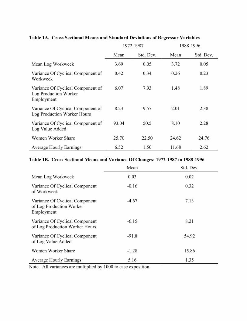
Table 1A. Cross Sectional Means and Standard Deviations of Regressor Variables

1972-1987 1988-1996

Mean Std. Dev. Mean Std. Dev.

Mean Log Workweek 3.69 0.05 3.72 0.05

Variance Of Cyclical Component ofWorkweek

0.42 0.34 0.26 0.23

Variance Of Cyclical Component ofLog Production WorkerEmployment

6.07 7.93 1.48 1.89

Variance Of Cyclical Component ofLog Production Worker Hours

8.23 9.57 2.01 2.38

Variance Of Cyclical Component ofLog Value Added

93.04 50.5 8.10 2.28

Women Worker Share 25.70 22.50 24.62 24.76

Average Hourly Earnings 6.52 1.50 11.68 2.62

Table 1B. Cross Sectional Means and Variance Of Changes: 1972-1987 to 1988-1996

Mean Std. Dev.

Mean Log Workweek 0.03 0.02

Variance Of Cyclical Componentof Workweek

-0.16 0.32

Variance Of Cyclical Componentof Log Production WorkerEmployment

-4.67 7.13

Variance Of Cyclical Componentof Log Production Worker Hours

-6.15 8.21

Variance Of Cyclical Componentof Log Value Added

-91.8 54.92

Women Worker Share -1.28 15.86

Average Hourly Earnings 5.16 1.35Note. All variances are multiplied by 1000 to ease exposition.

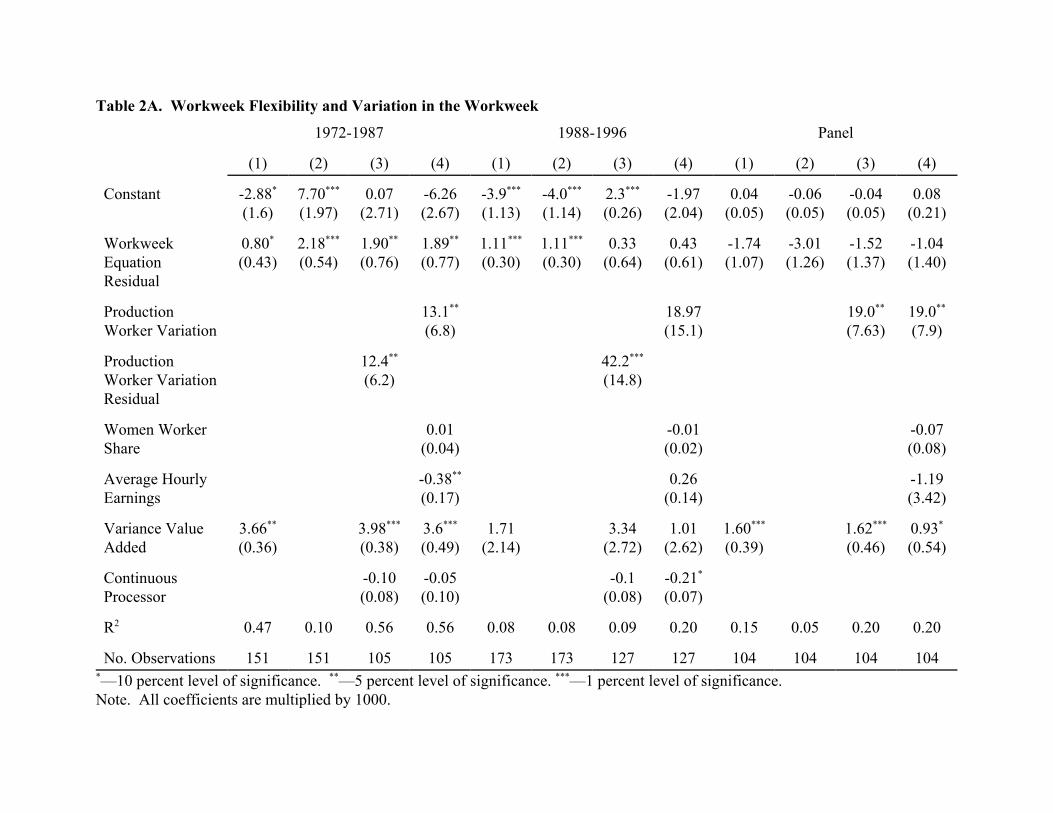
Table 2A. Workweek Flexibility and Variation in the Workweek

1972-1987 1988-1996 Panel

(1) (2) (3) (4) (1) (2) (3) (4) (1) (2) (3) (4)

Constant -2.88*

(1.6)7.70***

(1.97)0.07

(2.71)-6.26(2.67)

-3.9***

(1.13)-4.0***

(1.14)2.3***

(0.26)-1.97(2.04)

0.04(0.05)

-0.06(0.05)

-0.04(0.05)

0.08(0.21)

WorkweekEquationResidual

0.80*

(0.43)2.18***

(0.54)1.90**

(0.76)1.89**

(0.77)1.11***

(0.30)1.11***

(0.30)0.33

(0.64)0.43

(0.61)-1.74(1.07)

-3.01(1.26)

-1.52(1.37)

-1.04(1.40)

ProductionWorker Variation

13.1**

(6.8)18.97(15.1)

19.0**

(7.63)19.0**

(7.9)

ProductionWorker VariationResidual

12.4**

(6.2)42.2***

(14.8)

Women WorkerShare

0.01(0.04)

-0.01(0.02)

-0.07(0.08)

Average HourlyEarnings

-0.38**

(0.17)0.26

(0.14)-1.19(3.42)

Variance ValueAdded

3.66**

(0.36)3.98***

(0.38)3.6***

(0.49)1.71

(2.14)3.34

(2.72)1.01

(2.62)1.60***

(0.39)1.62***

(0.46)0.93*

(0.54)

ContinuousProcessor

-0.10(0.08)

-0.05(0.10)

-0.1(0.08)

-0.21*

(0.07)

R2 0.47 0.10 0.56 0.56 0.08 0.08 0.09 0.20 0.15 0.05 0.20 0.20

No. Observations 151 151 105 105 173 173 127 127 104 104 104 104*—10 percent level of significance. **—5 percent level of significance. ***—1 percent level of significance. Note. All coefficients are multiplied by 1000.

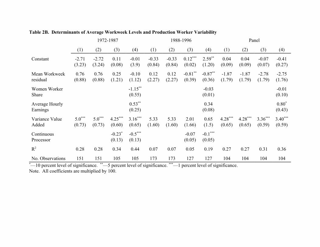
Table 2B. Determinants of Average Workweek Levels and Production Worker Variability

1972-1987 1988-1996 Panel

(1) (2) (3) (4) (1) (2) (3) (4) (1) (2) (3) (4)

Constant -2.71(3.23)

-2.72(3.24)

0.11(0.08)

-0.01(3.9)

-0.33(0.84)

-0.33(0.84)

0.12***

(0.02)2.59**

(1.20)0.04

(0.09)0.04

(0.09)-0.07(0.07)

-0.41(0.27)

Mean Workweekresidual

0.76(0.88)

0.76(0.88)

0.25(1.21)

-0.10(1.12)

0.12(2.27)

0.12(2.27)

-0.81**

(0.39)-0.87**

(0.36)-1.87(1.79)

-1.87(1.79)

-2.78(1.79)

-2.75(1.76)

Women WorkerShare

-1.15**

(0.55)-0.03(0.01)

-0.01(0.10)

Average HourlyEarnings

0.53**

(0.25)0.34

(0.08)0.80*

(0.43)

Variance ValueAdded

5.0***

(0.73)5.0***

(0.73)4.25***

(0.60)3.16***

(0.65)5.33

(1.60)5.33

(1.60)2.01

(1.66)0.65(1.5)

4.28***

(0.65)4.28***

(0.65)3.36***

(0.59)3.40***

(0.59)

ContinuousProcessor

-0.23*

(0.13)-0.5***

(0.13)-0.07(0.05)

-0.1***

(0.05)

R2 0.28 0.28 0.34 0.44 0.07 0.07 0.05 0.19 0.27 0.27 0.31 0.36

No. Observations 151 151 105 105 173 173 127 127 104 104 104 104*—10 percent level of significance. **—5 percent level of significance. ***—1 percent level of significance. Note. All coefficients are multiplied by 100.

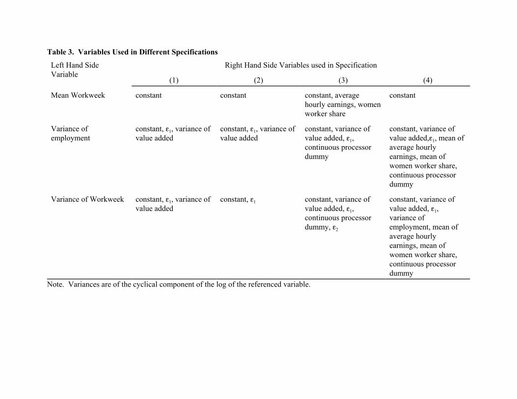
Table 3. Variables Used in Different Specifications

Left Hand SideVariable

Right Hand Side Variables used in Specification

(1) (2) (3) (4)

Mean Workweek constant constant constant, averagehourly earnings, womenworker share

constant

Variance ofemployment

constant, g1, variance ofvalue added

constant, g1, variance ofvalue added

constant, variance ofvalue added, g1,continuous processordummy

constant, variance ofvalue added,g1, mean ofaverage hourlyearnings, mean ofwomen worker share,continuous processordummy

Variance of Workweek constant, g1, variance ofvalue added

constant, g1 constant, variance ofvalue added, g1,continuous processordummy, g2

constant, variance ofvalue added, g1,variance ofemployment, mean ofaverage hourlyearnings, mean ofwomen worker share,continuous processordummy

Note. Variances are of the cyclical component of the log of the referenced variable.

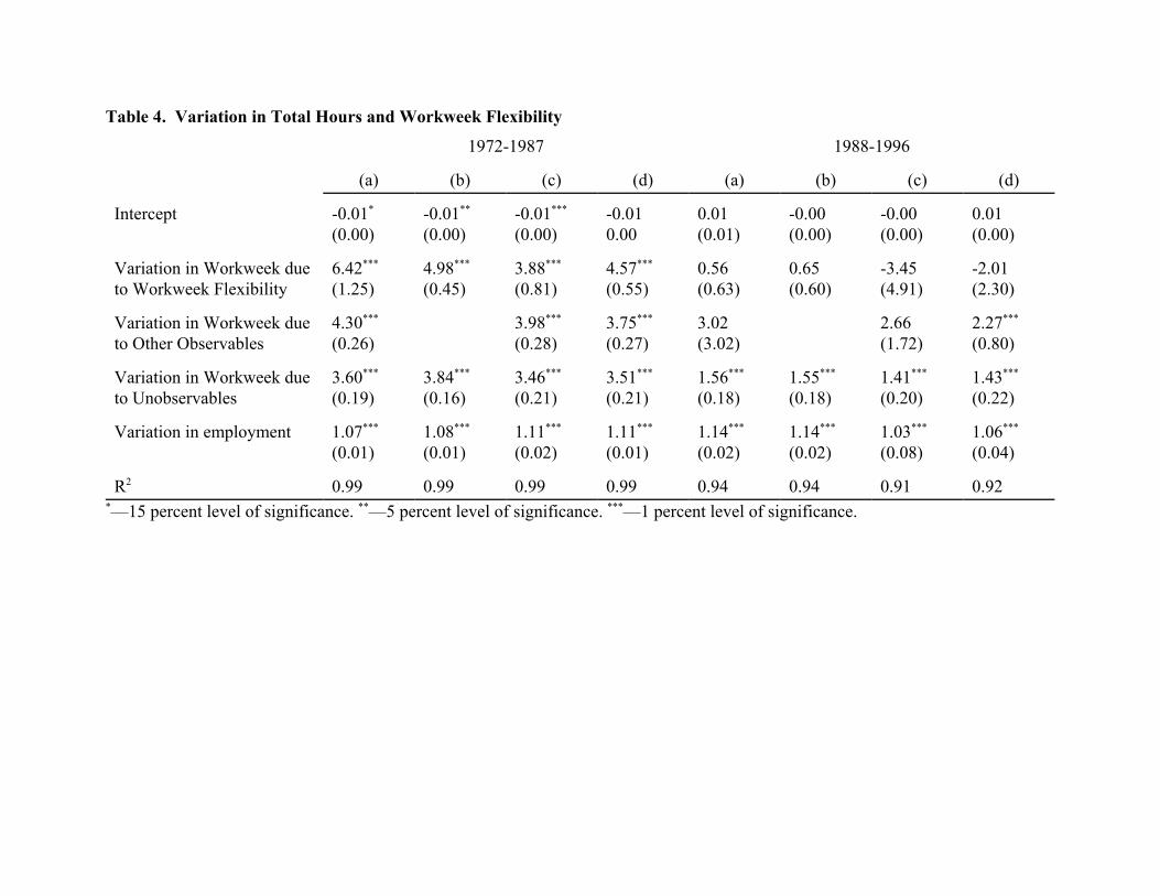
Table 4. Variation in Total Hours and Workweek Flexibility

1972-1987 1988-1996

(a) (b) (c) (d) (a) (b) (c) (d)

Intercept -0.01*

(0.00)-0.01**

(0.00)-0.01***

(0.00)-0.010.00

0.01(0.01)

-0.00(0.00)

-0.00(0.00)

0.01(0.00)

Variation in Workweek dueto Workweek Flexibility

6.42***

(1.25)4.98***

(0.45)3.88***

(0.81)4.57***

(0.55)0.56(0.63)

0.65(0.60)

-3.45(4.91)

-2.01(2.30)

Variation in Workweek dueto Other Observables

4.30***

(0.26)3.98***

(0.28)3.75***

(0.27)3.02(3.02)

2.66(1.72)

2.27***

(0.80)

Variation in Workweek dueto Unobservables

3.60***

(0.19)3.84***

(0.16)3.46***

(0.21)3.51***

(0.21)1.56***

(0.18)1.55***

(0.18)1.41***

(0.20)1.43***

(0.22)

Variation in employment 1.07***

(0.01)1.08***

(0.01)1.11***

(0.02)1.11***

(0.01)1.14***

(0.02)1.14***

(0.02)1.03***

(0.08)1.06***

(0.04)

R2 0.99 0.99 0.99 0.99 0.94 0.94 0.91 0.92*—15 percent level of significance. **—5 percent level of significance. ***—1 percent level of significance.

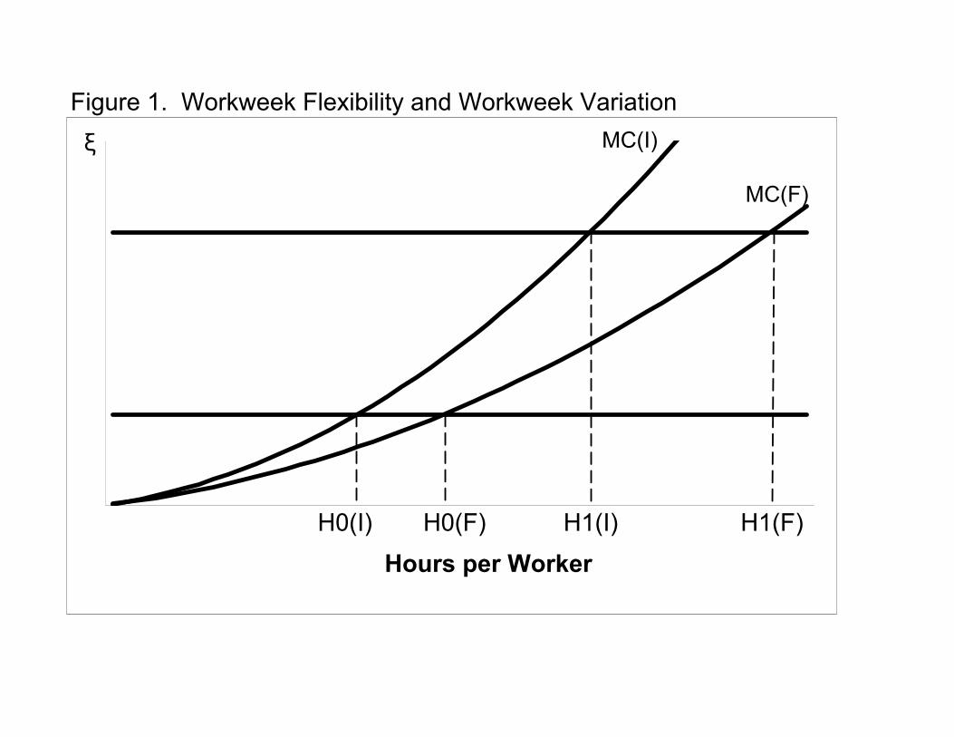
Figure 1. Workweek Flexibility and Workweek Variation

Hours per Worker

>

H0(I) H0(F) H1(I) H1(F)

MC(I)

MC(F)

Workweek

39

40

41

42

43

44

Year

1972

1976

1980

1984

1988

1992

1996

2000

2004

Percent Deviation

-20

-16

-12

-8

-4048

12

16

20

Year

1971

1974

1977

1980

1983

1986

1989

1992

1995

1998

2001