SP DISCUSSION PAPER NO. 0131

24081

Child Labor, Nutrition andEducation in Rural India:An Economic Analysis of Parental

q4 CiChoice and Policy Options

ITdK *5 Alessandro Cigno? 4t.~ WFurio Camillo Rosati

Zafiris Tzannatos

December 2001

FILE COPY &jV:rUontonLABOR MARKETS, PENSIONS, SOCIAL ASSISTANCE

T H E W O R L D B A N K

Pub

lic D

iscl

osur

e A

utho

rized

Pub

lic D

iscl

osur

e A

utho

rized

Pub

lic D

iscl

osur

e A

utho

rized

Pub

lic D

iscl

osur

e A

utho

rized

Pub

lic D

iscl

osur

e A

utho

rized

Pub

lic D

iscl

osur

e A

utho

rized

Pub

lic D

iscl

osur

e A

utho

rized

Pub

lic D

iscl

osur

e A

utho

rized

Child Labor, Nutrition and Education in Rural India:An Economic Analysis of Parental Choice and Policy Options

Alessandro CignoFurio Camillo Rosati

Zafiris Tzannatos

December, 2001

ABSTRACT

The causes and consequences of child labor are examined within a household decisionframework with survival uncertainty and endogenous fertility. The data come from anationally representative survey of Indian rural households. The complex interactionsuncovered by the analysis suggest that mere prohibition of child labor, or the imposition ofschool attendance, would make things worse, and would be difficult to enforce. Beneficiallyreducing child labor requires changing the economic environment to which the work ofchildren constitutes, in the great majority of cases, the rational response. Suitable policiesinclude capillary provision of schools, and public health improvements. The effects of thesepolicies go far beyond direct impacts. They have favorable indirect repercussions on theschool attendance, educational expenditure, labor participation, and nutritional status ofchildren. They also discourage fertility. Women's education, and income re-distribution arealso helpful, but land re-distribution may be counterproductive.

Keywords: child labor, education, fertility, mortality, anthropometry, household economic

Child Labor, Nutrition and Education in Rural India: An Economic Analysis ofParental Choice and Policy Options

Alessandro Cigno, Furio C. Rosati, Zafiris Tzannatos*

I. INTRODUCTION

Child labor is an emotive subject. Especially where very young children are

concerned, it evokes images of maltreatment and exploitation. Such cases do exist and call

for repressive measures, but there is not a great deal that the economist can say on the subject

(beyond pointing to a possible trade-off between severity of the sanction and probability of

detection). Quantitatively more important, however, are the cases where child labor is not

the result of criminal intent, but a well-meaning response to material poverty. It may well be

argued that, in these cases too, national governments and international agencies should do

something to reduce the extent of the phenomenon, but the arguments for intervention have

to be the standard ones: either some kind of coordination failure', which justifies public

intervention on efficiency grounds, or social preferences such that some form of

re-distribution (from parents to children, from rich to poor families, or from rich to poor

countries) is deemed desirable. Either way, one has to start with a representation of child

labor behavior, and of how this responds to policy.

Section 2 of the present paper provides an overview of child labor (or, more

generally, of child engagement in activities other than study and play) through a survey of

Indian households. Section 3 develops a theoretical framework for explaining the allocation

of a child's time, and related decisions regarding fertility and the allocation of household

budgets. Sections 4 and 5 contain an econometric analysis of the Indian data. Section 6

discusses the empirical findings in the light of the theory, and derives policy implications.

'The authors Alessandro Cigno, University of Florence, Furio Camillo Rosati, University of Rome "TorVergata" and Zafiris Tzannatos, The World Bank.'For an application of the argument to the present context, see Grootaert and Kanbur (1995).

II CHILD WORK, SCHOOLING AND WELFARE IN RURAL INDIA

Our data come from the Human Development of India Survey, carried out by the

National Council of Applied Economic Research (NCAER) of New Delhi. This is a

multi-purpose, nationally representative sample survey conducted during 1994 in the rural

areas of India. A two-stage stratified and partially selfweighting design was used to sample a

total of 34,398 households spread over 1,765 villages and 195 districts in 16 states. Two

separate survey instruments were devised, one to elicit the economic and income parameters

from an adult male member, and the other to collect data on outcomes such as literacy,

education, health, morbidity, nutrition, and demographic parameters from the adult female

members of the household. The data are representative of rural population at the level of all

India, according to states and population groups, and according to selected population groups

for the selected states. Information on child work is obtained merging the "Children" file,

relating to children aged 0-12, with information on individuals older than 12 years, contained

in the "Individuals" file. Information about household level variables was added by merging

the "Reproductive Information" file with the other two.

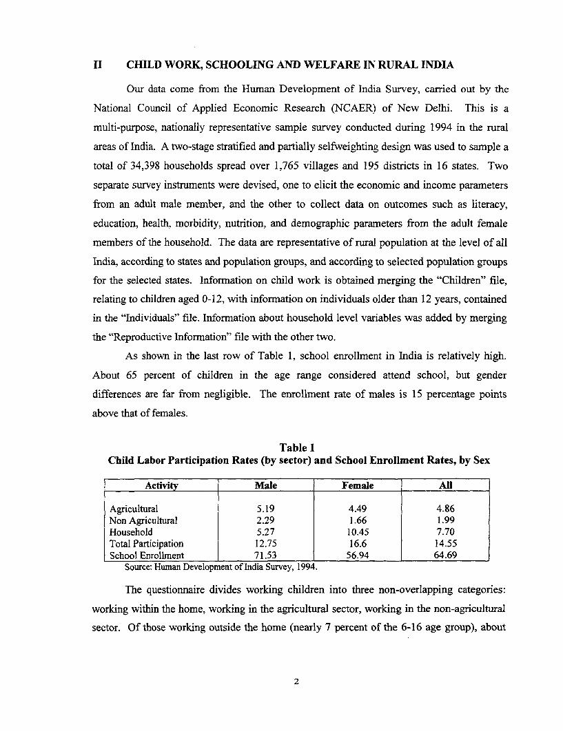
As shown in the last row of Table 1, school enrollment in India is relatively high.

About 65 percent of children in the age range considered attend school, but gender

differences are far from negligible. The enrollment rate of males is 15 percentage points

above that of females.

Table 1Child Labor Participation Rates (by sector) and School Enrollment Rates, by Sex

Activity Male Female All

Agricultural 5.19 4.49 4.86Non Agricultural 2.29 1.66 1.99Household 5.27 10.45 7.70Total Participation 12.75 16.6 14.55School Enrollment 71.53 56.94 64.69

Source: Human Development of India Survey, 1994.

The questionnaire divides working children into three non-overlapping categories:

working within the home, working in the agricultural sector, working in the non-agricultural

sector. Of those working outside the home (nearly 7 percent of the 6-16 age group), about

2

half are reported receiving wages (in money or in kind). We assume that the rest are

employed in the family (usually farm) business. As most of the children reported working

within the home are female, we assume that they perform household chores (including

assistance to younger children).

Table 1 shows that about 15 percent of children in the 6-16 age group is reported to be

engaged in paid or unpaid work. The household is the most common place of child work.

While gender differences are not particularly relevant where work performed outside the

home is concerned, the participation rate of girls in household work is twice as large as that

of boys. There are, therefore, more boys than girls reported as not working. The unbalance

reflects partly the fact that more of the boys go to school, but partly also the fact that more of

the boys are reported as neither attending school, nor working (more about this later).

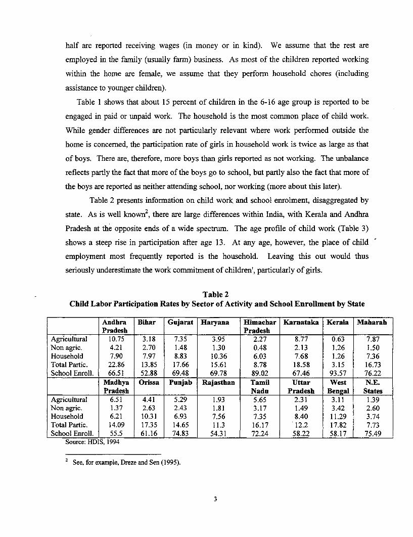
Table 2 presents information on child work and school enrolment, disaggregated by

state. As is well known2 , there are large differences within India, with Kerala and Andhra

Pradesh at the opposite ends of a wide spectrum. The age profile of child work (Table 3)

shows a steep rise in participation after age 13. At any age, however, the place of child

employment most frequently reported is the household. Leaving this out would thus

seriously underestimate the work commitment of children', particularly of girls.

Table 2Child Labor Participation Rates by Sector of Activity and School Enrollment by State

Andhra Bihar Gujarat Haryana Himachar Karnataka Kerala MaharahPradesh Pradesh

Agricultural 10.75 3.18 7.35 3.95 2.27 8.77 0.63 7.87Non agric. 4.21 2.70 1.48 1.30 0.48 2.13 1.26 1.50Household 7.90 7.97 8.83 10.36 6.03 7.68 1.26 7.36Total Partic. 22.86 13.85 17.66 15.61 8.78 18.58 3.15 16.73School Enroll. 66.51 52.88 69.48 69.78 89.02 67.46 93.57 76.22

Madhya Orissa Punjab Rajasthan Tamil Uttar West N.E.Pradesh Nadu Pradesh Bengal States

Agricultural 6.51 4.41 5.29 1.93 5.65 2.31 3.11 1.39Non agric. 1.37 2.63 2.43 1.81 3.17 1.49 3.42 2.60Household 6.21 10.31 6.93 7.56 7.35 8.40 11.29 3.74Total Partic. 14.09 17.35 14.65 11.3 16.17 12.2 17.82 7.73School Enroll. 55.5 61.16 74.83 54.31 72.24 58.22 58.17 75.49

Source: HDIS, 1994

2 See, for example, Dreze and Sen (1995).

3

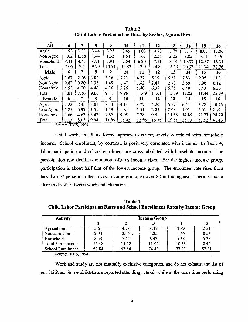
Table 3Child Labor Participation Ratesby Sector, Age and Sex

All 6 7 8 9 10 11 12 13 14 15 16Agric. 1.93 2.31 3.44 3.25 3.65 4.03 4.73 5.74 7.17 8.06 12.06Non Agric. 1.02 0.88 1.44 1.35 1.64 1.67 2.28 2.26 2.82 3.11 4.39Household 4.11 4.41 4.91 5.91 7.04 6.30 7.81 8.53 10.33 12.57 16.31Total 7.06 7.6 9.79 10.51 12.33 12.0 14.82 16.53 20.32 23.74 32.76

Male 6 7 8 9 10 11 12 13 14 15 16Agric. 1.67 2.16 3.82 3.36 3.23 4.27 5.19 5.81 7.83 9.05 13.31Non Agric. 0.82 0.80 1.38 1.49 1.47 1.82 2.47 2.43 3.59 3.96 6.12Household 4.52 4.20 4.46 4.26 5.26 5.40 6.35 5.55 6.40 5.43 6.56Total 7.01 7.16 9.66 9.11 9.96 11.49 14.01 13.79 17.82 18.44 25.99

Female 6 7 8 9 10 11 12 13 14 15 16Agric. 2.22 2.45 3.01 3.13 4.13 3.77 4.20 5.67 6.41 6.78 10.45Non Agric. 1.25 0.97 1.51 1.19 1.84 1.51 2.05 2.08 1.93 2.01 2.19Household 3.66 4.63 5.42 7.67 9.05 7.28 9.51 11.86 14.85 21.73 28.79Total 7.13 8.05 9.94 11.99 15.02 12.56 15.76 19.61 23.19 30.52 41.43

Source: HDIS, 1994

Child work, in all its forms, appears to be negatively correlated with household

income. School enrolment, by contrast, is positively correlated with income. In Table 4,

labor participation and school enrolment are cross-tabulated with household income. The

participation rate declines monotonically as income rises. For the highest income group,

participation is about half that of the lowest income group. The enrolment rate rises from

less than 57 percent in the lowest income group, to over 82 in the highest. There is thus a

clear trade-off between work and education.

Table 4Child Labor Participation Rates and School Enrollment Rates by Income Group

Activity Income Group1 2 3 4 5

Agricultural 5.61 4.73 3.37 3.59 2.51Non agricultural 2.34 2.05 1.25 1.26 0.53Household 8.53 7.44 6.43 5.68 5.38Total Participation 16.48 14.22 11.05 10.53 8.42School Enrollment 57.84 67.84 74.83 77.00 82.31

Source: HDIS, 1994

Work and study are not mutually exclusive categories, and do not exhaust the list of

possibilities. Some children are reported attending school, while at the same time performing

4

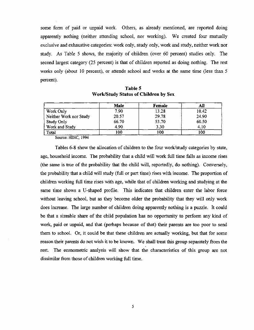
some form of paid or unpaid work. Others, as already mentioned, are reported doing

apparently nothing (neither attending school, nor working). We created four mutually

exclusive and exhaustive categories: work only, study only, work and study, neither work nor

study. As Table 5 shows, the majority of children (over 60 percent) studies only. The

second largest category (25 percent) is that of children reported as doing nothing. The rest

works only (about 10 percent), or attends school and works at the same time (less than 5

percent).

Table 5Work/Study Status of Children by Sex

Male Female AlUWork Only 7.90 13.28 10.42Neither Work nor Study 20.57 29.78 24.90Study Only 66.70 53.70 60.50Work and Study 4.90 3.30 4.10Total 100 100 100

Source: HDIC, 1994

Tables 6-8 show the allocation of children to the four work/study categories by state,

age, household income. The probability that a child will work full time falls as income rises

(the same is true of the probability that the child will, reportedly, do nothing). Conversely,

the probability that a child will study (full or part time) rises with income. The proportion of

children working full time rises with age, while that of children working and studying at the

same time shows a U-shaped profile. This indicates that children enter the labor force

without leaving school, but as they become older the probability that they will only work

does increase. The large number of children doing apparently nothing is a puzzle. It could

be that a sizeable share of the child population has no opportunity to perform any kind of

work, paid or unpaid, and that (perhaps because of that) their parents are too poor to send

them to school. Or, it could be that these children are actually working, but that for some

reason their parents do not wish it to be known. We shall treat this group separately from the

rest. The econometric analysis will show that the characteristics of this group are not

dissimilar from those of children working full time.

5

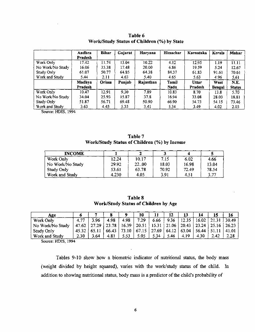
Table 6Work/Study Status of Children (%) by State

Andhra Bihar Gujarat Haryana Himachar Karnataka Kerala MaharPradesh

Work Only 17.42 11.74 13.04 10.22 4.12 12.95 1.19 11.11No Work/No Study 16.06 35.38 17.48 20.00 6.86 19.59 5.24 12.67Study Only 61.07 50.77 64.85 64.38 84.37 61.83 91.61 70.61U'ork and Study 5.44 2.11 4.63 5.40 4.65 5.63 4.96 5.61

Madhya Orissa Punjab Rajasthan Tamil Uttar West N.E.Pradesh Nadu Pradesh Bengal States

W ork Only 10.47 12.91 9.30 7.89 10.83 8.70 13.8 5.70No Work/No Study 34.04 25.93 15.87 37.8 16.94 33.08 28.03 18.81Study Only 51.87 56.71 69.48 50.90 66.90 54.73 54.15 73.46Work and Study 3.63 4.45 5.35 3.41 5.34 3.49 4.02 | 2.03

Source: HDIS, 1994

Table 7Work/Study Status of Children (%) by Income

INCOME 1 2 3 4 5Work Only 12.24 10.17 7.15 6.02 4.66No Work/No Study 29.92 22-00 18.03 16.98 13.04Study Only 53.61 63.78 70.92 72.49 78.54Work and Study 4.230 4.05 3.91 4.51 3.77

Table 8Work/Study Status of Children by Age

Age 6 7 8 9 10 11 12 13 14 15 16Work Only 4.77 3.96 4.98 4.98 7.29 6.66 9.36 12.35 16.02 21.31 30.49No Work/No Study 47.62 27.29 23.78 16.39 20.51 15.31 21.06 20.43 23.24 25.16 26.23Study Only 45.32 65.11 66.43 73.10 67.15 27.69 64.12 63.04 56.44 51.11 41.01Work and Study 2.30 3.64 4.81 j 5.53 5.05 5.34 5.46 4.19 4.30 2.42 2.28

Source: HDIS, 1994

Tables 9-10 show how a biometric indicator of nutritional status, the body mass

(weight divided by height squared), varies with the work/study status of the child. In

addition to showing nutritional status, body mass is a predictor of the child's probability of

6

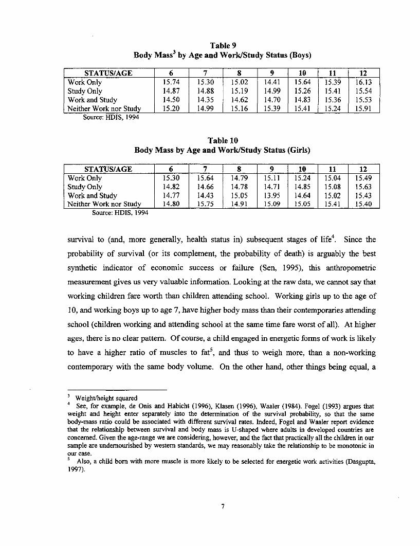
Table 9Body Mass3 by Age and Work/Study Status (Boys)

STATUS/AGE 6 7 8 9 10 11 12Work Only 15.74 15.30 15.02 14.41 15.64 15.39 16.13Study Only 14.87 14.88 15.19 14.99 15.26 15.41 15.54Work and Study 14.50 14.35 14.62 14.70 14.83 15.36 15.53Neither Work nor Study 15.20 14.99 15.16 15.39 15.41 15.24 15.91

Source: HDIS, 1994

Table 10Body Mass by Age and Work/Study Status (Girls)

STATUS/AGE 6 7 8 9 10 11 12Work Only 15.30 15.64 14.79 15.11 15.24 15.04 15.49Study Only 14.82 14.66 14.78 14.71 14.85 15.08 15.63Work and Study 14.77 14.43 15.05 13.95 14.64 15.02 15.43Neither Work nor Study 14.80 15.75 14.91 15.09 15.05 15.41 15.40

Source: HDIS, 1994

survival to (and, more generally, health status in) subsequent stages of life4. Since the

probability of survival (or its complement, the probability of death) is arguably the best

synthetic indicator of economic success or failure (Sen, 1995), this anthropometric

measurement gives us very valuable information. Looking at the raw data, we cannot say that

working children fare worth than children attending school. Working girls up to the age of

10, and working boys up to age 7, have higher body mass than their contemporaries attending

school (children working and attending school at the same time fare worst of all). At higher

ages, there is no clear pattern. Of course, a child engaged in energetic forms of work is likely

to have a higher ratio of muscles to fat5 , and thus to weigh more, than a non-working

contemporary with the same body volume. On the other hand, other things being equal, a

3 Weight/height squared4 See, for example, de Onis and Habicht (1996), Klasen (1996), Waaler (1984). Fogel (1993) argues thatweight and height enter separately into the deternination of the survival probability, so that the samebody-mass ratio could be associated with different survival rates. Indeed, Fogel and Waaler report evidencethat the relationship between survival and body mass is U-shaped where adults in developed countries areconcemed. Given the age-range we are considering, however, and the fact that practically all the children in oursample are undemourished by westem standards, we may reasonably take the relationship to be monotonic inour case.5 Also, a child born with more muscle is more likely to be selected for energetic work activities (Dasgupta,1997).

7

working child needs more food to reach any given body volume. It thus seems unlikely that,

of two children with the same sex, age and body mass, the one who works will have received

less nutrition than the one who does not.

To sum up, the data show that child work is an important phenomenon. How

important depends on what we call work: little important if we only count children reported

working for a wage or in the family business (7 percent), important (14 percent) if we add

those performing household chores, very important (over 39 percent) if we also include those

that are reported doing nothing, but which we suspect may be actually working. Working

children appear to fare better, in terms of current nutrition and future health, than children

who study; but will enter adulthood with a smaller stock of human capital than children who

study. Children who study will have more human capital, but probably poorer health, than

working children6 .

III AN EXPLANATORY FRAMEWORK

Assuming that infants and children are under the control of parents, any analysis of

why a child might work must start with a model of parental decisions. Since the decision of

whether or not to send a child to work is closely interrelated with that of whether or not to

send the child to school, of how much to spend for the child (and in which way) at various

points of the life cycle, and ultimately of how many children to have, all of these must

considered within a unified framework. We shall see that, not only the effects of policies

directly aimed at improving children's welfare, such as free or subsidized provision of school

facilities, but also those of more broadly aimed policies, such as sanitation or preventive

medicine, depend on how parental decisions are modified in response to such policies.

The decision problem has the following structure. Parents decide whether or not to

procure an extra birth7, and decide how much to spend for each pre-school child, under

conditions of uncertainty about whether he or she will reach school age. If the child survives,

6 While the trade-off between work and study is obviously one-to-one, the trade-off between the outputs ofthese activities (respectively, current consumption and future human capital or consumption) may be lower. Theevidence (e.g., Psacharopoulos, 1997; Patrinos and Psacharopoulos, 1997), however, is somewhat discordant.7 Strictly speaking, we should be saying that parents-to-be condition the probability distribution of an extrabirth by choosing the frequency of intercourse, whether to use contraception, etc. But, the mechanics of fertilitydetermination are not the focus of the present paper.

8

parents decide how much to spend for him or her, and how to allocate his or her time

between work and study8. We do not go into the issue of the balance of power between

father, mother and other adult family members at this stage, but we are aware that the weight

of the mother in decision making may rise (and the quality of decisions regarding child

welfare may improve) with her education and outside earnings. We shall come back to this

point in the interpretation of the empirical results.

We examine the issue in the context of two alternative models, one assuming altruism

and the other self-interest on the part of parents towards their children. Throughout, we

assume that parents control fertility, and condition the survival probability of their children at

various points of the life-cycle through expenditure on certain items. Since the model must

serve to explain household data on rural India, we allow for the possibility that parents own

or rent land.

Altruistic Model

The life-time utility of parents depends on their own life-time consumption, on the

consumption of their pre-school and school-age children, and on the amount of human capital

with which each of these children will enter adult life9. The list of goods consumed by

children includes food and medical care, but excludes educational inputs (which are

considered separately). The amount consumed in the pre-school period is assumed to have a

positive effect on the probability that the child will survive to school age and, more

generally, on his or her current and future health prospects. Since the amount that a person is

able to earn, as an adult, is positively related to the person's health (dependent on past

consumption) and personal skills (dependent on human capital), saying that parents care

8 Given the nature of the data we shall want to explain, it seemed reasonable to assume that the realcompetition for the use of the child's time is between work and study. Leisure (or playtime) is treated as aresidual, something that is done at times of the day, or of the year, when there is nothing else for children to do.9 Since time spent in education reduces time spent working hour-for-hour, the marginal rate of substitution ofhuman-capital for consumption may reflect not only willingness to trade present for future consumption, butalso physical complementarity between work and food consumption. Suppose, for example, that the marginalrate of substitution were 3. This might simply mean that the child (or his parents for him) is willing to give upthree units of present consumption in exchange for one unit of human capital (future consumption). Or, it couldbe the case that the child would have been willing to trade food for human capital one-for-one if work and studyhad the same calories requirement, but is actually willing to give up another two units of food on account of thefact that studying uses less calories than working.

9

about their children's current consumption and future human capital is equivalent to saying

that they care about their children's lifetime welfare.

Human capital is partly a reflection of native talent and partly the fruit of education.

The second part is "produced" with time (which includes not only school attendance, but also

study outside school hours), and other educational inputs (books, tuition and writing material,

but also travel to school). The opportunity cost of time spent in education is equal to the

child wage rate, or to the marginal product of child labor in the family farm, whichever is

higher. The marginal cost of human capital is constantl0 up to the point where the child's

time if fully employed in education. From that point onward, it increases with human capital,

as more and more has to be spent for educational inputs in conjunction with a fixed amount

of time.

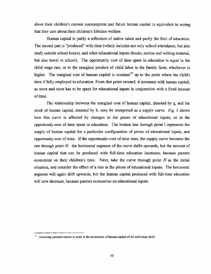
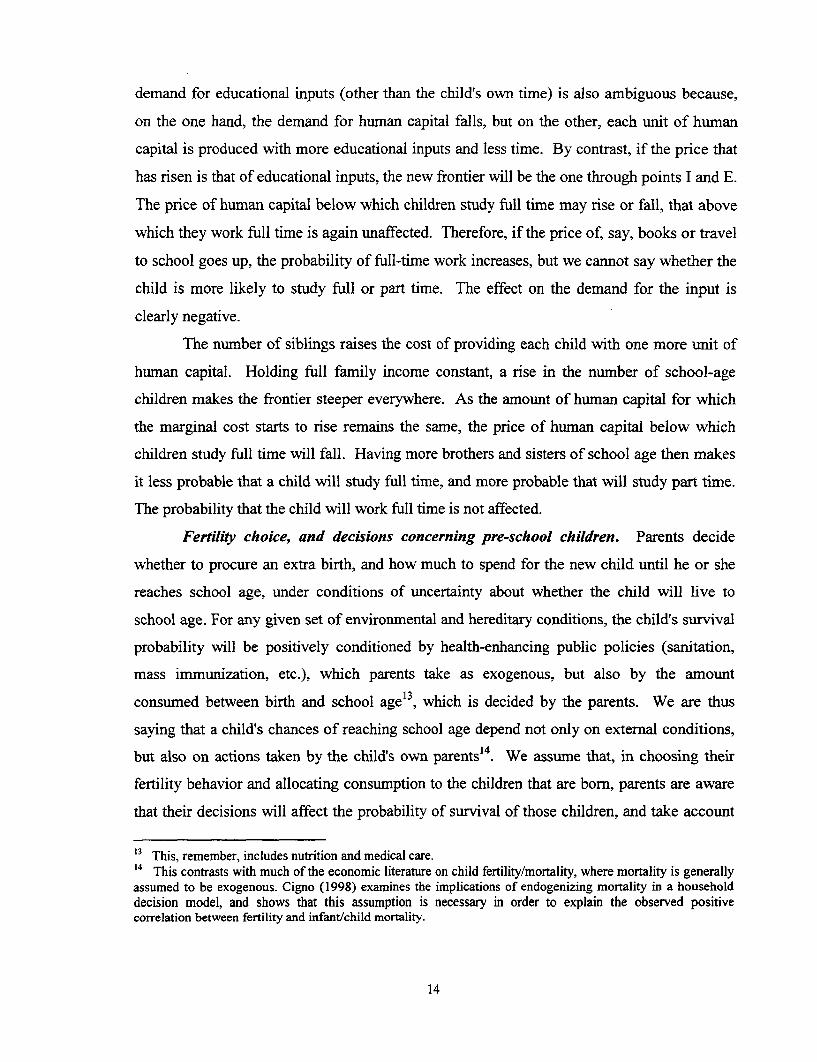
The relationship between the marginal cost of human capital, denoted by q, and the

stock of human capital, denoted by h, may be interpreted as a supply curve. Fig. I shows

how this curve is affected by changes in the prices of educational inputs, or in the

opportunity-cost of time spent in education. The broken line through point I represents the

supply of human capital for a particular configuration of prices of educational inputs, and

opportunity-cost of time. If the opportunity-cost of time rises, the supply curve becomes the

one through point H: the horizontal segment of the curve shifts upwards, but the amount of

human capital that can be produced with full-time education increases, because parents

economize on their children's time. Next, take the curve through point H as the initial

situation, and consider the effect of a rise in the prices of educational inputs. The horizontal

segment will again shift upwards, but the human capital produced with full-time education

will now decrease, because parents economize on educational inputs.

° Assuming constant retums to scale in the production of human capital of the individual child.

10

q H

Fig IDecsinscocenig /cholag i

Figr I

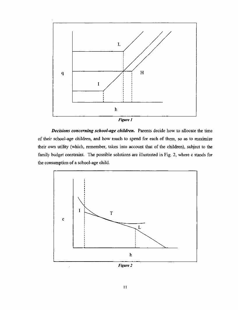
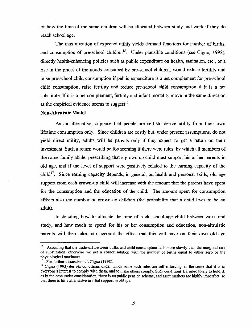
of their school-age children, and how much to spend for each of them, so as to maximize

their own utility (which, remember, takes into account that of the children), subject to the

family budget constraint. The possible solutions are illustrated in Fig. 2, where c stands for

the consumption of a school-age child.

cd

h

Figure 2

1 1

The broken line through points I and L is the production frontier. The abscissa of

point I is the amount of human capital that the child would have in the absence of education

("natural talent"). To the right of point L, the child's time is fully occupied in education. The

slope of the production frontier, equal to the marginal cost of human capital, is constant to

the left of point L, increasing to the right of it. The choice set is delimited by the vertical line

through point I to the left (parents cannot sell off their children's natural talent), and by the

production frontier upwards. The slope of the indifference curve through point I is the price

of human capital above which parents are not willing to bear any cost for their children's

education. The slope of the indifference curve through point L is the price of human capital

below which parents want their children to study full time.

The first type of solution is at point I, where the marginal cost of human capital is

higher than the maximum that parents are willing to pay. If that is the type of solution, the

child is made to work full time. The second type of solution is at any point between I and L

(e.g., at point T), where the marginal cost of human capital is equal to its marginal rate of

substitution for consumption. If that is the case, the child works and studies at the same time.

The third type of solution is either at or to the right of point L, where the marginal cost of

human capital is lower than the minimum below which parents want their children to study

full time. If that is the case, the child does not work at all. If parents send their children to

school at all, they also spend for educational inputs.

A lump-sum increase in family income raises current consumption and the future

stock of human capital for every child", but it also raises the maximum that parents are

willing to pay for an extra unit of human capital, and the minimum below which they want

their children to study full time. Since the marginal cost of human capital is not affected, the

probability that a child will work full time will then fall, while the probability that the child

studies full time will rise. The probability that the child works and studies may go either

way.

Assuming that consumption and human capital are normal goods.

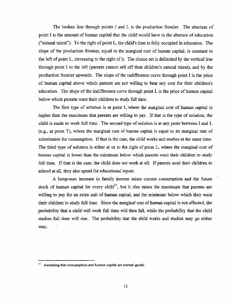
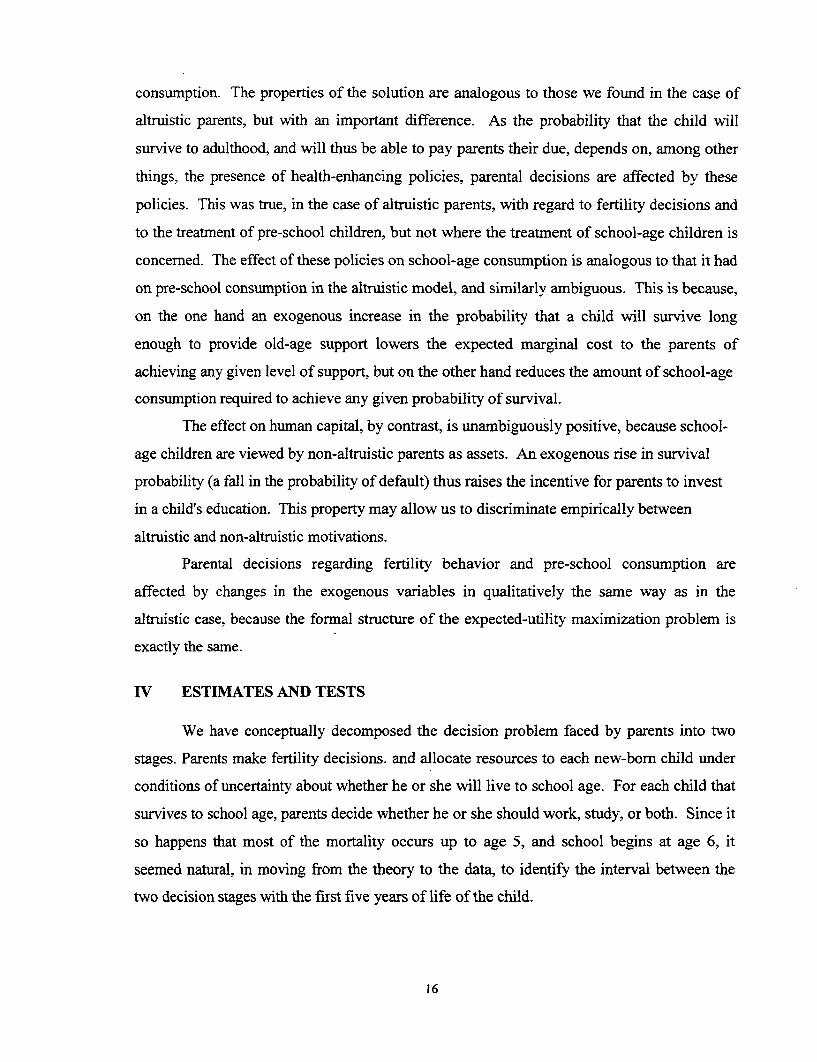
Fig. 3 illustrates the effects of an increase in the price of an educational input, or in

the opportunity-cost of time in education, holding full household income constant"2 . Take

h

Figure 3

the broken line through point L as the frontier before the change. By raising the marginal

cost of human capital, an increase in either of those variables makes the frontier steeper

everywhere. Unless the child already is a full-time worker (i.e., the initial solution happens

to be at point I), this will lead to a rise in the child's consumption. Other effects will depend

on whether the increase was in the opportunity-cost of time or in the price of an educational

input. If the former, the new frontier will be like the one through points I and H. As the

price of human capital below which parents want their children to study full time falls, and

that above which they want children to work full time stays the same, the effect of a rise in

the child wage rate (or, if the child works for his parents, in the domestic productivity of

child labor) is to raise the probability of full-time work, and to lower the probability of full-

time study; the effect on the probability of part-time work is ambiguous. The effect on the

12 That is to say, assuming a compensatory lump-sum transfer to the household if prices rise, from thehousehold if the opportunity-cost of time rises. The reason for holding income, rather than utility, constant isthat, as we have seen, the data contain income information, which we shall want to exploit.

13

demand for educational inputs (other than the child's own time) is also ambiguous because,

on the one hand, the demand for human capital falls, but on the other, each unit of human

capital is produced with more educational inputs and less time. By contrast, if the price that

has risen is that of educational inputs, the new frontier will be the one through points I and E.

The price of human capital below which children study full time may rise or fall, that above

which they work full time is again unaffected. Therefore, if the price of, say, books or travel

to school goes up, the probability of full-time work increases, but we cannot say whether the

child is more likely to study full or part time. The effect on the demand for the input is

clearly negative.

The number of siblings raises the cost of providing each child with one more unit of

human capital. Holding full family income constant, a rise in the number of school-age

children makes the frontier steeper everywhere. As the amount of human capital for which

the marginal cost starts to rise remains the same, the price of human capital below which

children study full time will fall. Having more brothers and sisters of school age then makes

it less probable that a child will study full time, and more probable that will study part time.

The probability that the child will work full time is not affected.

Fertility choice, and decisions concerning pre-school children. Parents decide

whether to procure an extra birth, and how much to spend for the new child until he or she

reaches school age, under conditions of uncertainty about whether the child will live to

school age. For any given set of environmental and hereditary conditions, the child's survival

probability will be positively conditioned by health-enhancing public policies (sanitation,

mass immunization, etc.), which parents take as exogenous, but also by the amount

consumed between birth and school age'3 , which is decided by the parents. We are thus

saying that a child's chances of reaching school age depend not only on external conditions,

but also on actions taken by the child's own parents14 . We assume that, in choosing their

fertility behavior and allocating consumption to the children that are born, parents are aware

that their decisions will affect the probability of survival of those children, and take account

13 This, remember, includes nutrition and medical care.14 This contrasts with much of the economic literature on child fertility/mortality, where mortality is generallyassumed to be exogenous. Cigno (1998) examines the implications of endogenizing mortality in a householddecision model, and shows that this assumption is necessary in order to explain the observed positivecorrelation between fertility and infant/child mortality.

14

of how the time of the same children will be allocated between study and work if they do

reach school age.

The maximization of expected utility yields demand functions for number of births,

and consumption of pre-school children'5 . Under plausible conditions (see Cigno, 1998),

directly health-enhancing policies such as public expenditure on health, sanitation, etc., or a

rise in the prices of the goods consumed by pre-school children, would reduce fertility and

raise pre-school child consumption if public expenditure is a net complement for pre-school

child consumption; raise fertility and reduce pre-school child consumption if it is a net

substitute. If it is a net complement, fertility and infant mortality move in the same direction

as the empirical evidence seems to suggest16 .

Non-Altruistic Model

As an alternative, suppose that people are selfish: derive utility from their own

lifetime consumption only. Since children are costly but, under present assumptions, do not

yield direct utility, adults will be parents only if they expect to get a return on their

investment. Such a return would be forthcoming if there were rules, by which all members of

the same family abide, prescribing that a grown-up child must support his or her parents in

old age, and if the level of support were positively related to the earning capacity of the

child' . Since earning capacity depends, in general, on health and personal skills, old age

support from each grown-up child will increase with the amount that the parents have spent

for the consumption and the education of the child. The amount spent for consumption

affects also the number of grown-up children (the probability that a child lives to be an

adult).

In deciding how to allocate the time of each school-age child between work and

study, and how much to spend for his or her consumption and education, non-altruistic

parents will then take into account the effect that this will have on their own old-age

15 Assuming that the trade-off between births and child consumption falls more slowly than the marginal rateof substitution, otherwise we get a corner solution with the number of births equal to either zero or thephysiological maximum.16 For further discussion, cf. Cigno (1998).17 Cigno (1993) derives conditions under which some such rules are self-enforcing, in the sense that it is ineveryone's interest to comply with them, and to make others comply. Such conditions are more likely to hold if,as in the case under consideration, there is no public pension scheme, and asset markets are highly imperfect, sothat there is little alternative to filial support in old age.

15

consumption. The properties of the solution are analogous to those we found in the case of

altruistic parents, but with an important difference. As the probability that the child will

survive to adulthood, and will thus be able to pay parents their due, depends on, among other

things, the presence of health-enhancing policies, parental decisions are affected by these

policies. This was true, in the case of altruistic parents, with regard to fertility decisions and

to the treatment of pre-school children, but not where the treatment of school-age children is

concerned. The effect of these policies on school-age consumption is analogous to that it had

on pre-school consumption in the altruistic model, and similarly ambiguous. This is because,

on the one hand an exogenous increase in the probability that a child will survive long

enough to provide old-age support lowers the expected marginal cost to the parents of

achieving any given level of support, but on the other hand reduces the amount of school-age

consumption required to achieve any given probability of survival.

The effect on human capital, by contrast, is unambiguously positive, because school-

age children are viewed by non-altruistic parents as assets. An exogenous rise in survival

probability (a fall in the probability of default) thus raises the incentive for parents to invest

in a child's education. This property may allow us to discriminate empirically between

altruistic and non-altruistic motivations.

Parental decisions regarding fertility behavior and pre-school consumption are

affected by changes in the exogenous variables in qualitatively the same way as in the

altruistic case, because the forrnal structure of the expected-utility maximization problem is

exactly the same.

IV ESTIMATES AND TESTS

We have conceptually decomposed the decision problem faced by parents into two

stages. Parents make fertility decisions. and allocate resources to each new-born child under

conditions of uncertainty about whether he or she will live to school age. For each child that

survives to school age, parents decide whether he or she should work, study, or both. Since it

so happens that most of the mortality occurs up to age 5, and school begins at age 6, it

seemed natural, in moving from the theory to the data, to identify the interval between the

two decision stages with the first five years of life of the child.

16

Where school-age children are concerned, the model predicts how much a child

consumes, and the probability that the child will work or study (part or full time), as

functions of full household income, number of siblings, marginal cost of human capital,

opportunity-cost of time spent in education, and various policy variables. It also makes

predictions regarding educational expenditure. Where pre-school children are concerned, the

model predicts fertility (the demand for births) and the consumption of each child as

functions of full household income, price of child-specific goods, and health-enhancing

policy variables, as well as of all the variables that will later affect decisions on school-age

children.

We estimated equations predicting the probability that a school-age child will work

full time or part time, educational expenditure for each child attending school, consumption

by pre-school and school-age children, and the probability of an extra birth. Time use by

school-age children is represented by a variable taking value 1 if the child is reported

working and not attending school, 2 if the child goes to school and works, 3 if the child

attends school and does not work (we shall come to the no-work, no-school category in a

moment). Demand for educational inputs (other than time) is represented by educational

expenditure per child attending school. Having no direct information on consumption by

children of either age group, we proxied consumption by the body mass index, which, as

mentioned in Section II, is at once a measure of nutritional status, and a predictor of the

probability of survival to the next stage of life. Fertility is represented by a dichotomous

variable taking value 1 if a birth occurred in the two years' 8 preceding the interview, 0 if it

did not.

The explanatory variables reflect, as closely as data permit, those figuring in the

theoretical analysis. Descriptive statistics are reported in Table 11.

Income is measured as the sum of the value of own-farm production and outside

earnings by all household members, including school-age children. Subsidiary income

information is provided by Tenure and Poverty. The former is a dichotomous variable,

taking value 1 if the household owns the land it works, 0 if it does not. The latter is an

Is Two rather than one because there is a certain margin of error in the recording of the exact date of birth ofeach child (and also because it gives us more observations).

17

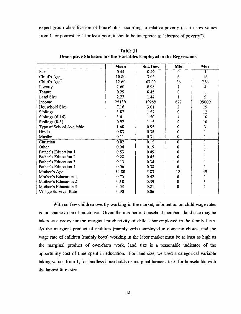
expert-group classification of households according to relative poverty (as it takes values

from 1 for poorest, to 4 for least poor, it should be interpreted as "absence of poverty").

Table 11Descriptive Statistics for the Variables Employed in the Regressions

Mean Std. Dev. Min MaxSex 0.44 0.49 0 1Child's Age 10.80 3.03 6 16Child's Age2 12.60 67.00 36 256Poverty 2.60 0.98 1 4Tenure 0.29 0.45 0 ILand Size 2.23 1.44 1 5Income 25139 19259 677 99000Household Size 7.16 3.01 2 19Siblings 3.82 1.57 0 12Siblings (6-16) 3.01 1.50 1 10Siblings (0-5) 0.92 1.15 0 10Type of School Available 1.60 0.95 0 3Hindu 0.83 0.38 0 1Muslim 0.11 0.31 0 1Christian 0.02 0.15 0 1Other 0.04 0.19 0 1Father's Education 1 0.53 0.49 0 1Father's Education 2 0.28 0.45 0 1Father's Education 3 0.13 0.34 0 1Father's Education 4 0.06 0.38 0 1Mother's Age 34.80 5.83 18 49Mother's Education 1 0.75 0.42 0 1Mother's Education 2 0.18 0.39 0 1Mother's Education 3 0.03 0.21 0 1Village Survival Rate 0.90 0.06

With so few children overtly working in the market, information on child wage rates

is too sparse to be of much use. Given the number of household members, land size may be

taken as a proxy for the marginal productivity of child labor employed in the family farm.

As the marginal product of children (mainly girls) employed in domestic chores, and the

wage rate of children (mainly boys) working in the labor market must be at least as high as

the marginal product of own-farm work, land size is a reasonable indicator of the

opportunity-cost of time spent in education. For land size, we used a categorical variable

taking values from 1, for landless households or marginal farmers, to 5, for households with

the largest farm size.

18

Individual and household characteristics are represented by the age (Age and Age

Squared) and sex (taking value 1 for a girl, 0 for a boy) of the child, the mother's age,

dummies describing the level of education of the child's father and mother (respectively,

Father's education i and Mother's education i, where i takes value 4 for completed high

school or higher, 3 for middle school, 2 for primary, 1 for less than primary), total number of

household members (Household size), number of pre-school children (Siblings 0 - 5), and

number of school-age children (Siblings 6 - 16). Where age structure is not significant, we

use the total number of children (Siblings). We also use dummies for the religion (Hindu,

Muslim, etc.) of the household head' 9.

Health policies and local environmental conditions are proxied by the village level

aggregate survival rate to age 6 (Village survival rate). By using this as a regressor, we are in

effect saying that parental action (and household characteristics) cause a dispersion of

individual probabilities of survival around the village-level mean20. As the mean of the

village survival rates is around 90%, there is clearly plenty of scope for parental action to

improve the survival chances of their own children. In view of the high degree of correlation

among survival rates to all ages, this variable is also a predictor of aggregate survival rates to

subsequent ages.

The effect on fertility is particularly important because its sign gives information on

whether the health policies proxied by the aggregate survival rate are a substitute or a

complement for parental expenditure on pre-school children. In the absence of statistical

information on the price of child-specific goods, which also would convey information on the

matter, that is all we have to go by.

Educational policies are represented by the variable School available, which takes

value 0 if there is no school in the village where the child lives, 1 if there is only a primary

school, 2 if there is a primary and a middle school, 3 if there is also a high school. The

19 Caste (represented by the variable Social) was also tried, but proved significant in only a few regressions.20 Ideally, we would want to get at the information, up to the date of conception of each child, that helped formparental expectations of these village means. That would require a large panel data set. As that is not available,we decided to exploit cross-sectional variations in survival data at village level. We computed village-levelmean survival rates from individual data. If cross-village differences have not changed widely over time, ourestimates should be a reasonably good measure of inter-village differences in parental expectations. Since, forsome villages, there are only a few individual observations, we also computed and tried district-level survivalmeans to check the robustness of our results. Results were unchanged.

19

presence of a school ready at hand constitutes a reduction in the price of educational inputs.

State dummies (Andhra Pradesh, Bihar, etc.) allow for other differences of policy, as well as

of climate, ethnic mix, etc.

Since, as mentioned in Section II, we are not sure about the real status of children

reported as neither attending school nor working, we exclude these children from the

estimates presented in this section. The characteristics of the "missing children" will be

examined in a section of their own.

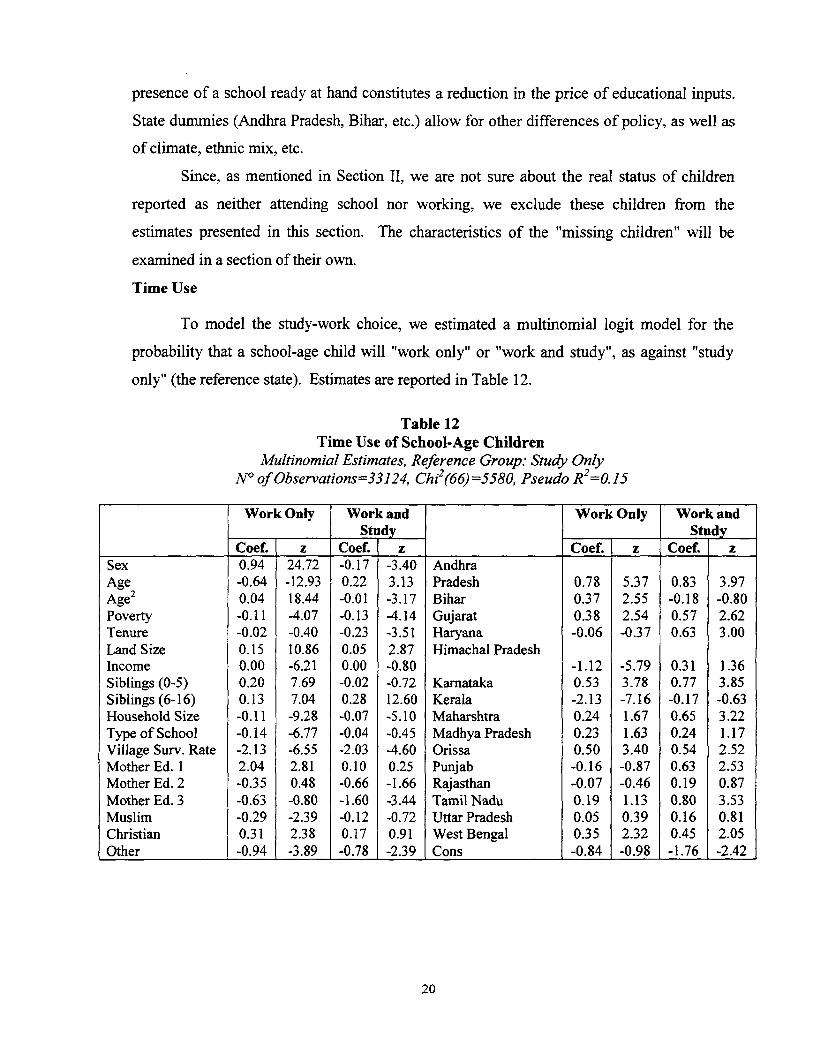
Time Use

To model the study-work choice, we estimated a multinomial logit model for the

probability that a school-age child will "work only" or "work and study", as against "study

only" (the reference state). Estimates are reported in Table 12.

Table 12Time Use of School-Age Children

Multinomial Estimates, Reference Group: Study OnlyN° of Observations=33124, Chi2 (66) =5580, Pseudo R2 = 0. 15

Work Only Work and Work Only Work andStudy Study

Coef. z Coef. z Coef. z Coef. zSex 0.94 24.72 -0.17 -3.40 AndhraAge -0.64 -12.93 0.22 3.13 Pradesh 0.78 5.37 0.83 3.97Age2 0.04 18.44 -0.01 -3.17 Bihar 0.37 2.55 -0.18 -0.80Poverty -0.11 -4.07 -0.13 -4.14 Gujarat 0.38 2.54 0.57 2.62Tenure -0.02 -0.40 -0.23 -3.51 Haryana -0.06 -0.37 0.63 3.00Land Size 0.15 10.86 0.05 2.87 Himachal PradeshIncome 0.00 -6.21 0.00 -0.80 -1.12 -5.79 0.31 1.36Siblings (0-5) 0.20 7.69 -0.02 -0.72 Kamataka 0.53 3.78 0.77 3.85Siblings (6-16) 0.13 7.04 0.28 12.60 Kerala -2.13 -7.16 -0.17 -0.63Household Size -0.11 -9.28 -0.07 -5.10 Maharshtra 0.24 1.67 0.65 3.22Type of School -0.14 -6.77 -0.04 -0.45 Madhya Pradesh 0.23 1.63 0.24 1.17Village Surv. Rate -2.13 -6.55 -2.03 -4.60 Orissa 0.50 3.40 0.54 2.52Mother Ed. 1 2.04 2.81 0.10 0.25 Punjab -0.16 -0.87 0.63 2.53Mother Ed. 2 -0.35 0.48 -0.66 -1.66 Rajasthan -0.07 -0.46 0.19 0.87Mother Ed. 3 -0.63 -0.80 -1.60 -3.44 Tamil Nadu 0.19 1.13 0.80 3.53Muslim -0.29 -2.39 -0.12 -0.72 Uttar Pradesh 0.05 0.39 0.16 0.81Christian 0.31 2.38 0.17 0.91 West Bengal 0.35 2.32 0.45 2.05Other -0.94 -3.89 -0.78 -2.39 Cons -0.84 -0.98 -1.76 -2.42

20

Girls are more likely to specialize fully in either work or education than to do both,

and more likely to specialize in work than boys21. The probability of working full time is

decreasing in age for children up to 8 years old, increasing for older children. The

probability of studying and working at the same time increases with age up to the 12th year,

then decreases.

Consistently with the theory, the estimated coefficients of the various income

measures indicate that belonging to a richer household reduces the probability- of working.

Land size raises the probability that a child will work (relative to not working at all), and the

probability that work will be full time rather than part time. Since land size proxies the

opportunity cost of time in education, this too is consistent with the theory, and provides

valuable indirect information on the return to child labor. The effects of household size and

composition are more complex.

An increase in total household size reduces the probability that a school-age child will

work at all, and makes it more likely that work will be part time. With the number of

children (up to age 16) controlled for, this is the same as saying that the number of adults in

the household reduces the probability of a child working. This is another labor productivity

effect: the greater the number of adults working on a given piece of land, the lower the return

to getting another child to work on it.

The number of pre-school children raises the probability that a school-age child will

"work only", relative to the probability that the child will "study only", but has no significant

effect on the probability of "work and study"22. Given that pre-school children are too young

to work, and that an increase in their number is thus equivalent to a lump-sum reduction in

full income (an income-dilution effect), this finding is consistent with the theoretical

prediction that a lump-sum increase in full income raises the probability of full-time work,

lowers that of full-time study, and has ambiguous effect on that of part-time work.

21 A "bootstraps" explanation is provided in Cigno (1991, Ch.5). Parents perceive the return to educating girlsas lower than the return to educating boys, because they observe that women are less likely to work, and thus toprofit from their education, than men. Women work less than men, however, because they are less educatedand, therefore, in the marital division of labor, have a comparative advantage in specializing in housework.

22 Patrinos and Psacharopooulos (1997) find the same in Peru.

21

The number of school-age children raises the probability that a child in that same age

range will "work only" or "work and study", but the effect on the probability of "work only"

is not as large as that of the number of pre-school children. That is consistent with the

theory, according to which an increase in the number of school-age children, holding full

income constant, raises the probability of part-time work, and lowers that of full-time study,

but has no effect on that of full-time work (while the number of pre-school children reduces

it).

The probability that a child will study full time increases with the presence of a

school in the village, and with the grade of education this school offers. These are price

effects. Having a school of any grade ready at hand reduces the marginal cost of, and thus

raises the demand for that grade of education. The fact that having a higher-grade school in

the village raises the probability of attending not only that grade of school, but also the lower

grades, requires some explanation. Drawing on evidence from Ghana, Lavy (1996)

maintains that returns to completing primary education and stopping there are low relative to

completing secondary and higher education. A lower cost of access to secondary education

thus increases the returns to investing in primary education. To check the validity of this

inference, we re-estimated the model for children aged 6 to 15 using two separate dummies,

one for the presence of a primary school, the other for the presence of a higher level school.

Since the coefficients of both these dummies have positive sign, the interpretation seems

legitimate. These findings are consistent with the theoretical predictions of both the altruistic

or the non-altruistic model, that a reduction in the price of education raises the probability of

going to school, and lowers the probability of working.

Consistently with the theoretical prediction of the non-altruistic model, the

village-level aggregate survival rate has a positive effect on the probability of studying full

time (relative to working full or part time). Therefore, public policies (sanitation, mass

immunization, etc.) aimed at improving the health and survival rates of children have the

desirable side-effect of inducing more parents to send their children to school. We shall see

in Section V that, as is to be expected, this effect is not present when children attending

school are excluded from the sample. Since this effect is not present in the altruistic model,

this finding may be taken as an indication that the non-altruistic model (see Section III)

22

provides the more appropriate explanatory framework for the phenomenon under

consideration.

The mother's own level of education appears to influence the decision to make a child

work or study. Children whose mothers have less than primary education are more likely to

work full time, than to study full time. Children whose mothers have more than primary

education are less likely to work and study than to study full time. By contrast, the father's

education does not exert a significant influence. With total household income controlled for,

the explanation for the effect of the mother's education has to be found outside the theoretical

framework presented in Section III.

A possible explanation is that education confers on the mother greater weight (moral

authority or, if education translates into income, bargaining power) in family decisions. If, as

some assume, mothers care for their children more than their fathers do, the mother's

education tends to increase the welfare of children (Folbre, 1986). Given the trade-off

between education and current consumption, however, this does not necessarily mean that

children of more educated mothers are more likely to go to school. Indeed, depending on

circumstances, caring mothers might insist on their children working, and the additional

income being used for the children's nutrition, rather than education.

Another consideration is that education increases the probability that the mother will

find outside employment, and thus that her children will be called upon to substitute for her

at the home (Basu, 1993). That is particularly true of girls who, if they do work, are likely to

do so within the home (looking after younger siblings, or in some other way substituting for

their mothers in the performance of domestic chores).

Yet another possibility is that the mothers time is an input into the education

(production of human capital) of their children, and that the mother's own level of education

raises the productivity of this input. According to this argument (Behrman et al., 1999), the

mother's own level of education raises the demand for her services as a home tutor, rather

than as a market laborer, and thus raises the return to the time that her children spend in

education. The possible coexistence of some or all of these mechanisms may explain the

finding of an effect of the mother's education on the probability that her children will go to

school, but also that this effect is not as pervasive as sometimes assumed (the probability of

23

full-time work is not affected by educational levels above, and that of part-time work by

educational levels below, completed primary education).

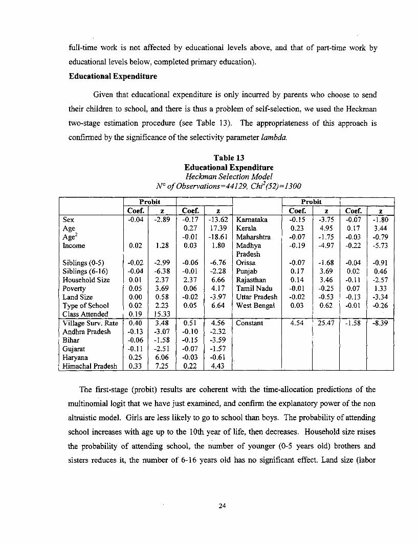
Educational Expenditure

Given that educational expenditure is only incurred by parents who choose to send

their children to school, and there is thus a problem of self-selection, we used the Heckman

two-stage estimation procedure (see Table 13). The appropriateness of this approach is

confirmed by the significance of the selectivity parameter lambda.

Table 13Educational ExpenditureHeckman Selection Model

N° of Observations=44129, Chi2 (52) =1300

Probit ProbitCoef. z Coef. z Coef. z Coef. z

Sex -0.04 -2.89 -0.17 -13.62 Karnataka -0.15 -3.75 -0.07 -1.80Age 0.27 17.39 Kerala 0.23 4.95 0.17 3.44Age2 -0.01 -18.61 Maharshtra -0.07 -1.75 -0.03 -0.79Income 0.02 1.28 0.03 1.80 Madhya -0.19 -4.97 -0.22 -5.73

PradeshSiblings (0-5) -0.02 -2.99 -0.06 -6.76 Orissa -0.07 -1.68 -0.04 -0.91Siblings (6-16) -0.04 -6.38 -0.01 -2.28 Punjab 0.17 3.69 0.02 0.46Household Size 0.01 2.37 2.37 6.66 Rajasthan 0.14 3.46 -0.11 -2.57Poverty 0.05 3.69 0.06 4.17 Tamil Nadu -0.01 -0.25 0.07 1.33Land Size 0.00 0.58 -0.02 -3.97 Uttar Pradesh -0.02 -0.53 -0.13 -3.34Type of School 0.02 2.23 0.05 6.64 West Bengal 0.03 0.62 -0.01 -0.26Class Attended 0.19 15.33Village Surv. Rate 0.40 3.48 0.51 4.56 Constant 4.54 25.47 -1.58 -8.39Andhra Pradesh -0.13 -3.07 -0.10 -2.32Bihar -0.06 -1.58 -0.15 -3.59Gujarat -0.11 -2.51 -0.07 -1.57Haryana 0.25 6.06 -0.03 -0.61Himachal Pradesh 0.33 7.25 0.22 4.43

The first-stage (probit) results are coherent with the time-allocation predictions of the

multinomial logit that we have just examined, and confirm the explanatory power of the non

altruistic model. Girls are less likely to go to school than boys. The probability of attending

school increases with age up to the 10th year of life, then decreases. Household size raises

the probability of attending school, the number of younger (0-5 years old) brothers and

sisters reduces it, the number of 6-16 years old has no significant effect. Land size (labor

24

productivity) reduces the probability of going to school, household income increases it.

School availability (and grade), and the village-level aggregate survival rate, also have a

positive effect.

The second-stage estimates show that the level of educational expenditure, given that

the child goes to school, is lower if the child is female, and increases with the grade of school

attended2 3, household income, the village-level aggregate survival rate, and school

availability. As was to be expected, land size is not significant, because labor productivity

(the opportunity-cost of time spent in education) affects the decision to send a child to

school, not how much to spend given that the child is going to school.

The positive effect of the aggregate survival rate on the probability and level of

educational expenditure is coherent with the finding of a positive effect of this variable on

the decision to send a child to school, and makes it more likely that the model generating the

data is non-altruistic (see Sub-Section 3.2).

Nutrition and Anthropometry

With age and sex controlled for, body mass is an indicator of nutritional status24 , but

also, as pointed out in Section II, a predictor of individual survival probability. Following

advice from the anthropometric literature25 , we estimated separate equations for pre-school

and school-age children.

Table 14 shows the results for school-age children26 . Their nutritional status appears

to be higher in richer households (Income and Tenure are not significant, but Poverty, i. e.

being less poor, has a significantly positive effect). For any given household income and

size, children with more brothers and sisters have lower body mass (an income dilution

23 In the second (level) stage of the estimation procedure, it seemed more appropriate to substitute age withschool grade, which reflects not only age, but also other factors (e.g., talent. past morbidity, etc..) affectingschool achievement.24 In this respect, the body mass index could be an overestimate or an underestimate. On the one hand,children performing physical work are likely to have more muscle, and thus to appear better fed, than theirbrothers engaged in sedentary activities like studying. On the other, working children expend more calories,and thus require more food to achieve the same body weight. Similar ambiguities occur in the interpretation ofsex differences. The negative coefficient of Sex in tables 16 and 17 indicates that girls have lower bodymassthan boys of the same age. But, constitutionally, girls tend to have less muscle than boys. It is thus not clearwhether the observed difference in body mass can be taken as evidence of sex discrimination in theintra-household allocation of nutrients (see Behrman, 1988), or of phyisiological differences between the sexes.25 For example, de Onis and Habicht (1996), Klasen (1996), Waaler (1984).26 Since height and weight information is only available for children aged up to 12, school age is re-defined,for present purposes, as 6-12.

25

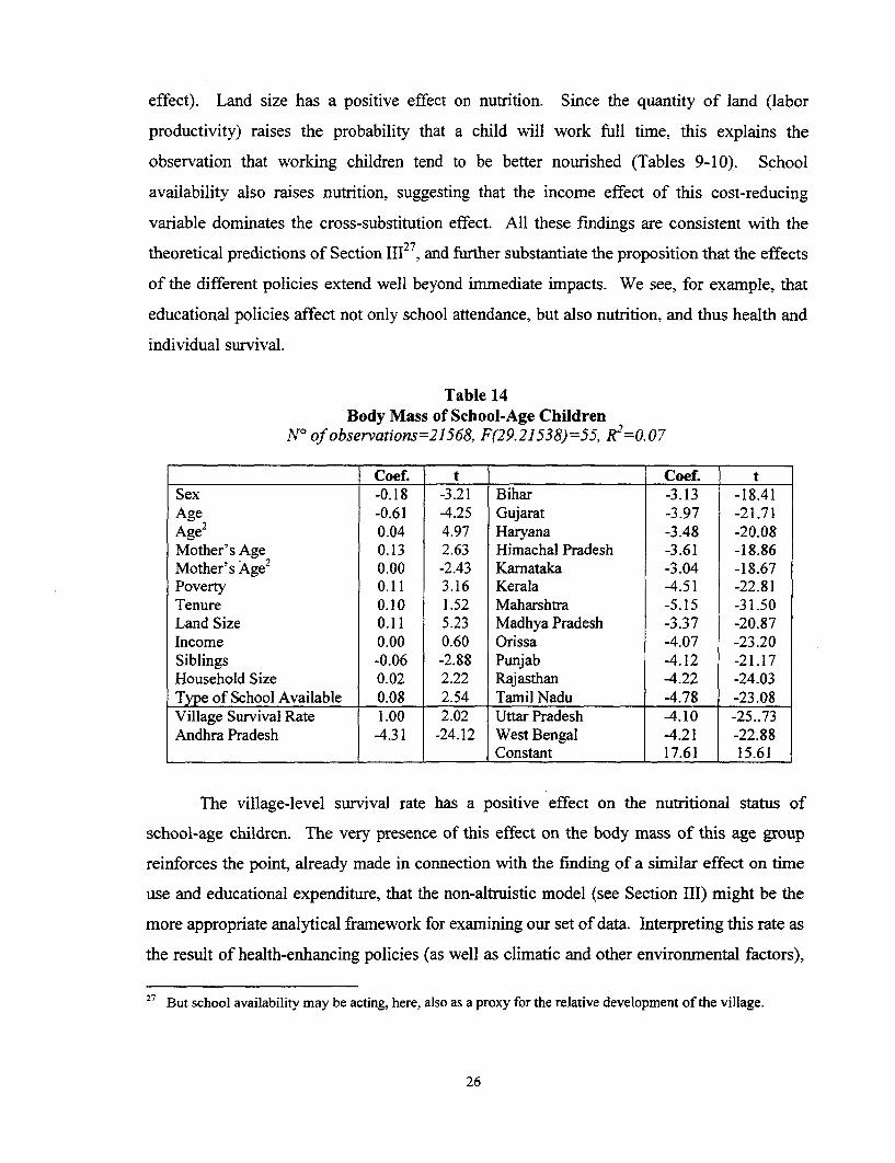
effect). Land size has a positive effect on nutrition. Since the quantity of land (labor

productivity) raises the probability that a child will work full time, this explains the

observation that working children tend to be better nourished (Tables 9-10). School

availability also raises nutrition, suggesting that the income effect of this cost-reducing

variable dominates the cross-substitution effect. All these findings are consistent with the

theoretical predictions of Section 11127, and firther substantiate the proposition that the effects

of the different policies extend well beyond immediate impacts. We see, for example, that

educational policies affect not only school attendance, but also nutrition, and thus health and

individual survival.

Table 14Body Mass of School-Age Children

Ni of observations=21568, F(29.21538) =55, R2=0. 07

Coef. t Coef. tSex -0.18 -3.21 Bihar -3.13 -18.41Age -0.61 -4.25 Gujarat -3.97 -21.71Age2 0.04 4.97 Haryana -3.48 -20.08Mother's Age 0.13 2.63 Himachal Pradesh -3.61 -18.86Mother's Age2 0.00 -2.43 Kanataka -3.04 -18.67Poverty 0.11 3.16 Kerala -4.51 -22.81Tenure 0.10 1.52 Maharshtra -5.15 -31.50Land Size 0.11 5.23 Madhya Pradesh -3.37 -20.87Income 0.00 0.60 Orissa -4.07 -23.20Siblings -0.06 -2.88 Punjab -4.12 -21.17Household Size 0.02 2.22 Rajasthan -4.22 -24.03Type of School Available 0.08 2.54 Tamil Nadu -4.78 -23.08Village Survival Rate 1.00 2.02 Uttar Pradesh -4.10 -25..73Andhra Pradesh -4.31 -24.12 West Bengal -4.21 -22.88

Constant 17.61 15.61

The village-level survival rate has a positive effect on the nutritional status of

school-age children. The very presence of this effect on the body mass of this age group

reinforces the point, already made in connection with the finding of a similar effect on time

use and educational expenditure, that the non-altruistic model (see Section III) might be the

more appropriate analytical framework for examining our set of data. Interpreting this rate as

the result of health-enhancing policies (as well as climatic and other environmental factors),

27 But school availability may be acting, here, also as a proxy for the relative development of the village.

26

the finding of a positive effect tells us that private expenditure is a net complement for public

expenditure. As pointed out in the theoretical discussion, this has the important policy

implication that public action stimulates and is reinforced by private (parental) action.

Biometric measures of pre-school children (not reported) are much less reliable than

for the older age-group. All explanatory variables, other than age, sex and state, have very

low levels of significance.

For both age groups, the state dummies have highly significant effects on nutritional

status. No doubt, these effects pick up climatic and ethnic differences (other things being

equal, children are likely to be more strongly built in Punjab, than in Maharashtra). The sign

pattern (children fare better in Andhra Pradesh than in Kerala) does, however, suggest that

they may also reflect differences in state policies, other than those accounted for by the

survival rate or the availability of schools at the village level.

To account for genetic differences not reflected in observed household characteristics,

we re-estimated the equations allowing for household-level random and fixed effects, but it

made no difference.

Fertility

For the probability of an extra birth, we estimated a probit model. The explanatory

variables include, in addition to those used for the other estimates, also the order of birth, and

the proportion of school-age children (in the household) who work. The latter is intended to

serve as a proxy for the probability that the structure of incentives facing the household when

the new-born child reaches school age will be such, that he or she will be made to work. The

results are shown in Table 15.

27

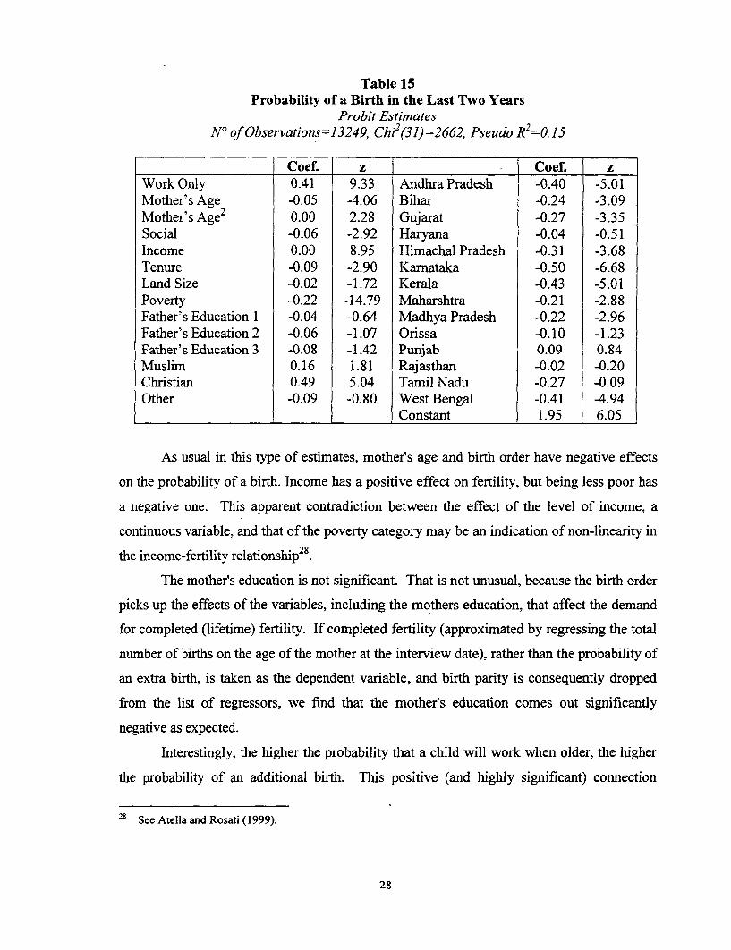
Table 15Probability of a Birth in the Last Two Years

Probit EstimatesN° of Observations=13249, Chi2 (31) =2662, Pseudo R2=0. 15

Coef. z Coef. zWork Only 0.41 9.33 Andhra Pradesh -0.40 -5.01Mother's Age -0.05 -4.06 Bihar -0.24 -3.09Mother's Age2 0.00 2.28 Gujarat -0.27 -3.35Social -0.06 -2.92 Haryana -0.04 -0.51Income 0.00 8.95 Himachal Pradesh -0.31 -3.68Tenure -0.09 -2.90 Karnataka -0.50 -6.68Land Size -0.02 -1.72 Kerala -0.43 -5.01Poverty -0.22 -14.79 Maharshtra -0.21 -2.88Father's Education 1 -0.04 -0.64 Madhya Pradesh -0.22 -2.96Father's Education 2 -0.06 -1.07 Orissa -0.10 -1.23Father's Education 3 -0.08 -1.42 Punjab 0.09 0.84Muslim 0.16 1.81 Rajasthan -0.02 -0.20Christian 0.49 5.04 Tamil Nadu -0.27 -0.09Other -0.09 -0.80 West Bengal -0.41 -4.94

_______ Constant 1.95 6.05

As usual in this type of estimates, mother's age and birth order have negative effects

on the probability of a birth. Income has a positive effect on fertility, but being less poor has

a negative one. This apparent contradiction between the effect of the level of income, a

continuous variable, and that of the poverty category may be an indication of non-linearity in

the income-fertility relationship2 8 .

The mother's education is not significant. That is not unusual, because the birth order

picks up the effects of the variables, including the mothers education, that affect the demand

for completed (lifetime) fertility. If completed fertility (approximated by regressing the total

number of births on the age of the mother at the interview date), rather than the probability of

an extra birth, is taken as the dependent variable, and birth parity is consequently dropped

from the list of regressors, we find that the mother's education comes out significantly

negative as expected.

Interestingly, the higher the probability that a child will work when older, the higher

the probability of an additional birth. This positive (and highly significant) connection

28 See Atella and Rosati (1999).

28

between fertility and probability of work brings further support to the hypothesis that the data

are generated by a non-altruistic model, because it suggests that parents may be looking for

an extra source of income, or for an extra pair of arms.

Availability of schools and the village-level survival rate are not significant, and are

excluded from the estimates. That is hardly surprising, in view of the fact that we are using as

a regressor the probability of full-time work if the child reaches school age, because we know

from the time-use estimates that this probability is significantly affected by the availability of

schools, and by the rate of survival at the village level. The finding of a positive effect of the

probability that the new-born child will work full time when of school age on the probability

of an extra birth, combined with the finding of negative effects of school availability and the

village-level survival rate on the probability of full-time work by school-age children, seems

to indicate that pro-education policies and public health improvements discourage fertility29 .

V. THE MISSING CHILDREN

It is difficult to dismiss the case of school-age children reported as neither working

nor attending school as a mere oversight. Local experts argue that, in certain circumstances,

children have such low productivity that it is not worth employing them in any work activity,

and that (partly as a consequence) their parents are too poor to send them to school. That

may well be the case, but we do not find it plausible that so many children, one in four, are

left totally idle by choice. It is thus worth investigating whether their characteristics bear any

similarities with those of children reported doing something.

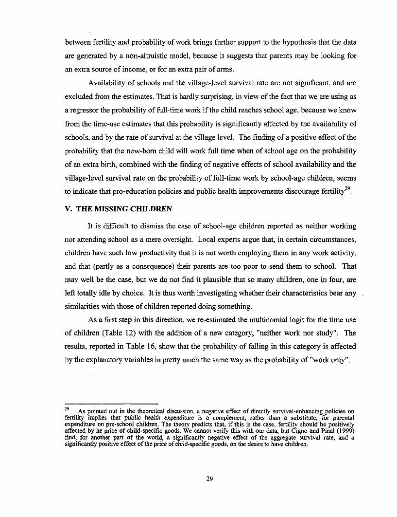
As a first step in this direction, we re-estimated the multinomial logit for the time use

of children (Table 12) with the addition of a new category, "neither work nor study". The

results, reported in Table 16, show that the probability of falling in this category is affected

by the explanatory variables in pretty much the same way as the probability of "work only".

29 As pointed out in the theoretical discussion, a negative effect of directly survival-enhancing policies onfertility implies that public health expenditure is a complement, rather than a substitute, for parentalexpenditure on pre-school children. The theory predicts that, if this is the case, fertility should be positivelyaffected by he price of child-specific goods. We cannot verify this with our data, but Cigno and Pinal (1999)find, for another part of the world, a significantly negative effect of the aggregate survival rate, and asignificantly positive effect of the price of child-specific goods, on the desire to have children.

29

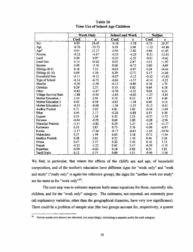
Table 16Time Use of School Age Children

Work Only School and Work NeitherCoef. z Coe£ z Coef. z

Sex 0.90 24.45 -0.18 -3.58 0.75 29.57Age -0.76 -15.72 0.19 2.68 -1.32 -41.86Age2 0.05 21.27 -0.01 -2.83 0.06 41.83Poverty -0.12 -4.47 -0.13 4.20 -0.21 -12.61Land 0.00 0.07 -0.23 -3.52 -0.01 -0.42Land Size 0.14 10.62 0.05 2.87 0.11 11.97Income 0.00 -5.76 0.00 -0.73 0.00 4.69Siblings (0-5) 0.18 7.15 -0.03 -0.87 0.24 14.44Siblings (6-16) 0.09 5.30 0.29 12.71 0.17 14.00Household Size -0.11 -9.15 -0.07 -5.13 -0.12 -15.92Type of School -0.14 -6.73 -0.04 -1.37 -0.14 -9.25Muslim -0.30 -2.50 -0.13 -0.80 0.16 1.70Christian 0.29 2.27 0.15 0.82 0.64 6.28Other -0.82 -3.47 -0.76 -2.32 0.04 0.24Village Survival Rate -1.88 -5.93 -2.03 -4.60 -1.27 -5.85Mother Education 1 2.14 2.94 0.13 0.33 1.47 4.30Mother Education 2 0.42 0.58 -0.63 -1.58 0.06 0.16Mother Education 3 -0.53 -0.68 -1.56 -3.35 -0.15 -0.41Andhra Pradesh 0.71 5.02 0.81 3.83 -0.36 -3.69Bihar 0.44 3.17 -0.20 -0.88 0.55 6.30Gujarat 0.35 2.38 0.55 2.53 -0.37 -3.72Haryana -0.04 -0.29 0.60 2.89 -0.28 -2.96Himachal Pradesh -1.11 -5.82 0.29 1.27 -1.54 -11.77Kamataka 0.53 3.87 0.75 3.76 -0.09 -0.97Kerala -2.17 -7.36 - -0.17 -0.61 -1.65 -10.94Maharshtra 0.21 1.49 0.65 3.18 -0.71 -7.44Madhya Pradesh 0.28 2.05 0.22 1.10 0.44 5.26Orissa 0.47 3.37 0.52 2.43 0.10 1.13Punjab -0.23 -1.23 0.62 2.47 -0.39 -3.10Rajasthan -0.09 -0.62 0.18 0.82 0.51 5.83Tamil Nadu 0.12 0.75 0.80 3.51 -0.40 -3.56

We find, in particular, that where the effects of the child's sex and age, of household

composition, and of the mother's education have different signs for "work only" and "work

and study" ("study only" is again the reference group), the signs for "neither work nor study",30are the same as for "work only"

The next step was to estimate separate body-mass equations for these, reportedly idle,

children, and for the "work only" category. The estimates, not reported, are extremely poor

(all explanatory variables, other than the geographical dummies, have very low significance).

There could be a problem of sample size (the two groups account for, respectively, a quarter

30 Similar results (not shown) are obtained, not surprisingly, estimating a separate probit for each category.

30

and a tenth of the total child population), or something specifically to do with these

categories of children. Although it is extremely unsafe to draw inferences from such

estimates, it is nonetheless worth reporting that, as in the time-use estimates just examined,

the sign pattem is the same for both categories of children. Most importantly, where there is

a sign difference between the "work only" equation and the equation estimated putting

together all children except those reportedly doing nothing, the sign in "neither work nor

study" is the same as in "work only". This strengthens the impression that the two groups

may be one and the same thing or, at least, that the "neither work nor study" category

contains a substantial proportion of children who are actually working full time.

VI. POLICY IMPLICATIONS

The empirical analysis of sections IV and V shows a high degree of consonance

among the estimates, and between these and the theoretical framework (particularly in its

non-altruistic version) of Section III. Taken together, the two levels of analysis prompt a

number of considerations. A very general one is that child labor cannot be viewed in

isolation from educational, health and fertility issues. Another is that, barring extreme

forms of exploitation (difficult to detect in the data), child labor should not be regarded as

an aberration, but rather as the rational household response to an adverse economic

environment - and, notice, this is true irrespective of whether parents are moved by altruistic

or selfish motivations. We now go on to examine the specific policy implications of our

analysis.

(i) Forbidding children to work or making school attendance compulsory, would, if

effectively enforced, reduce school-age consumption, and discourage fertility.

We have found that children working full time tend to have better nutritional status

than children who study, and that children who attend school and work at the same time fare

worst of all. Therefore, the policy would have ambiguous effect on the welfare of children

(who would end up with more human capital, but poorer health), and negative effect on the

welfare of their parents (forced to depart from their optimal choices). Parents would

consequently be tempted to evade the rules. Prohibiting work or insisting on school

attendance, without changing the economic environment that makes child work and

31

non-school attendance in the interest of the parents, and possibly of the child, is thus difficult

to enforce. It is possibly not in the interest of society either3 '. We have identified a number

of policies that would change the environment in the desired direction. Table 17 shows the

marginal effects, calculated at the sample mean, of a number of policy variables. Table 18

simulates the effects of more radical policy changes, consisting of raising a policy variable

from its minimum to its maximum value.

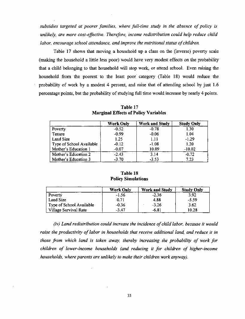
(ii) Capillary school provision reduces the incidence of child labor, and raises

educational expenditure for school attendants. It also discourages fertility, and improves

child nutrition.

The specific measure on the effects of which we have empirical evidence is that of

providing schools at village level. Nearly all villages (95 percent) have at least a primary

school. Table 17 shows that providing a middle school to a village where there was only a

primary one would reduce the probability that a schoolage child works by 1.2 percentage

points. Raising provision from nothing to secondary level (Table 18) would raise the

probability of full-time school attendance by 3.6 percentage points, mainly because of the

reduction of the number of children that both work and attend school32. These effects are

very important in themselves, and also because, as we have seen, the presence of a school

nearby, and the consequent reduction in the probability that a school-age child will work,

induce parents to procure fewer births, and to better feed and care for each child.

Furthermore, every school-age child that attends school attracts higher educational

expenditure. School provision affects, therefore, much more than education: it improves

school attendance, but also reduces child work (the two, remember, are not mutually

exclusive) and is likely to reduce morbidity and mortality through the lifecycle.

(iii) Universal income subsidies for parents are an expensive way of discouraging

child labor, because some of the subsidy will end up as adult consumption, and a

countereffective one in families where children would otherwise study full time. Income

3' Basu (1999) argues that prohibition to employ children would be beneficial (and self-enforcing, once thenew equilibrium is in place) if the labor market had two possible equilibria, one with low wage rate andemployment of children, the other with high wage rate and only adults employed. That is indeed true, but thevery fact that prohibition has not worked where it has been tried suggests that the assumption of a virtuousequilibrium waiting to be implemented may not hold universally. Furthermore, it seems scarcely relevant inour context, where the overwhelming majority of the children that work is reported working in the home or inthe family farm.32 See also Rosati and Tzannatos (1999).

32

subsidies targeted at poorer families, where full-time study in the absence of policy is

unlikely, are more cost-effective. Therefore, income redistribution could help reduce child

labor, encourage school attendance, and improve the nutritional status of children.

Table 17 shows that moving a household up a class on the (inverse) poverty scale

(making the household a little less poor) would have very modest effects on the probability

that a child belonging to that household will stop work, or attend school. Even raising the

household from the poorest to the least poor category (Table 18) would reduce the

probability of work by a modest 4 percent, and raise that of attending school by just 1.6

percentage points, but the probability of studying full time would increase by nearly 4 points.

Table 17Marginal Effects of Policy Variables

Work Only Work and Study Study OnlyPoverty -0.52 -0.78 1.30Tenure -0.99 -0.06 1.04Land Size 1.25 1.11 -1.29Type of School Available -0.12 -1.08 1.20Mother's Education 1 -0.07 10.09 -10.02Mother's Education 2 -2.43 3.14 -0.72Mother's Education 3 -3.70 -3.53 7.23

Table 18Policy Simulations

Work Only Work and Study Study OnlyPoverty -1.56 -2.36 3.92Land Size 0.71 4.88 -5.59Type of School Available -0.36 -3.26 3.62Village Survival Rate -3.47 -6.81 10.28

(iv) Land redistribution could increase the incidence of child labor, because it would

raise the productivity of labor in households that receive additional land, and reduce it in

those from which land is taken away, thereby increasing the probability of work for

children of lower-income households (and reducing it for children of higher-income

households, where parents are unlikely to make their children work anyway).

33

At the mean, bringing the quantity of land farmed by the household up one class

raises the probability that a school-age child will work by 1.4 percentage points. The

probability of school attendance falls hardly at all, but that of full-time study becomes 1.3

percents lower. The probability that a child belonging to a household with a farm in the top

size class will work is about 5 percentage points higher, other things being equal, than that of

a child belonging to a landless or marginal farming household (Table 18).

(v) Survival-enhancing policies reduce the probability that a school-age child will

work and raise the probability that the child will go to school. They also raise school-age

consumption, and the amount spent for the education of each school attendant.

The effects of these policies are captured in our data by the village-level survival

rate. Raising this rate from the minimum, 60 percent, to the maximum, 100 percent (i.e.,

deploying health policies such that children receiving from their parents the average amount

of nutrition and health care are certain to live at least to age 6) would reduce the probability

that a school-age child is sent to work by more than 10 percents, and raise that of full time

school attendance by the same amount (Table 18). In the same way as the effects of

education policy extend beyond education, so the effects of health policy (public

expenditure on sanitation, mass immunization, etc.) thus extend beyond health3 3. The

policy in question lowers the probability that a child will work, and raises the probability

that a child will be sent to school. Indeed, these side-effects of public health policy appear

to be rather powerful. The reason is, as we have seen, that the policy induces parents to

spend more not only for the education, but also for the nutrition of each school attendant.

The policy thus reduces morbidity and mortality not only directly, but also indirectly

through induced parental action. The finding of an effect on parental decisions conceming

children in this age-group is a symptom that the household decision model generating our

data may be non-altruistic.

(vi) Raising the education of women has positive but uneven effects on school

attendance, and school-age work It has no effect on fertility, nutrition, and educational

expenditure per school attendant.

33 Our empirical fndings are broadly consistent with those of Rosenzweig and Wolpin (1982), who also adopta household economics framework. but are not directly concerned with child labor.

34

In general, the education of women is a powerful engine of progress. Where school

enrolment and school-age work in rural India is concerned, however, it appears to be an

important, but probably not crucial factor (see Table 17). Raising the mother's education

from less than completed to completed primary school level would reduce the probability of

her children working by almost 9 percentage points, and raise the probability that they will

study full time by the same percentage. Raising her education from primary to

middle-school level would reduce the probability that her children work by over 7 percentage

points. As pointed out in Section IV, the reason for this uneven pattern may be that the

mother's education affects decisions about the allocation of her children's time in several

different and, in some respects, conflicting ways.

A word, finally, about the so-called missing children, those reported neither working,

nor attending school. Despite expert opinion that many of these children really do nothing, or

very little, we have found signs that a sizeable proportion of them may be actually working

full time. Their nutritional status is reported to be, on average, better than that of children

attending school, and no worse than that of children reported working full time, but

additional information and a more thorough statistical analysis are required before any firm

conclusion can be reached.

35

REFERENCES

Atella, V. and F.C. Rosati (1999) "Uncertainty About Children's Survival and Fertility: ATest Using Indian Microdata", Washington, DC. World Bank SP Discussion Paper No.9931, December 1999

Basu, A.M. (1993) "Family Size and Child Welfare in an Urban Slum" in C.B. Lloyd (ed.)Fertility, Family Size and Structure, Population Council, New York

Basu, K. (1999) "Child Labor: Cause, Consequence and Cure, with Remarks onInternational Labor Standards", Journal of Economic Literature 37, pp. 1083-1119

Becker, G.S. and H.G. Lewis (1973) "On the Interaction between the Quantity and Quality ofChildren", Journal of Political Economy 81, pp. 279-288

Behrman, J. (1988) "Intrahousehold Allocation of Nutrients in Rural India: Are BoysFavored?", Oxford Economic Papers 40, pp. 32-54

Behrman, J., Foster, A.D., Rosenzweig, M.R. and P. Vashishtha (1999) "Women'sSchooling, Home Teaching, and Economic Growth", Journal of Political Economy 107, pp.683-714

Cigno, A. (1991) Economics of the Family, Clarendon Press and Oxford University Press,Oxford and New York

Cigno, A. (1993) "Intergenerational Transfers without Altruism: Family, Market and State",European Journal of Political Economy 7, pp. 505-518

Cigno, A. (1998) "Fertility Decisions when Infant Survival is Endogenous", Journal ofPopulation Economics 11, pp.2 1 -28

Cigno, A. and C. Pinal (1999) "Endogenous Child Mortality, Price of Child-Specific Goods,and Fertility Decisions: Evidence From the Argentinian Andes", IEA World Congress,Buenos Aires

Dasgupta, P. (1997) "Nutritional Status, the Capacity for Work, and Poverty Traps", JournalOf Econometrics 77, pp. 5-37

de Onis, M. and J.P. Habicht (1996) "Anthropometric Reference Data for International Use:Recommendations from a World Health Organization Expert Committee", American JournalOf Clinical Nutrition 64, pp. 650-658

Dreze, J. and A. Sen (1995) India: Economic Development and Social Opportunity,Clarendon Press, Oxford

36

Fogel, R.W. (1993) "New Sources and New Techniques for the Study of Secular Trends inNutritional Status, Health, Mortality, and the Process of Aging", Historical Methods 26, pp.5-43

Folbre, N. (1986) "Hearts and Spades: Paradigms of Household Economics", WorldDevelopment 14, pp. 245-255

Grootaert, C. and R. Kanbur (1995), "Child Labor: An Economic Perspective", InternationalLabor Review 134, pp. 187-203

Klasen, S. (1996) "Nutrition, Health and Mortality in Sub-Saharan Africa: Is There a GenderBias?" Journal of Development Studies 32, pp. 913-32

Lavy, V. (1996) " School Supply Constraints and Children's Educational Outcomes in RuralGhana", Journal of Development Economics 51, pp. 291-314

Murthi, M., Guio, A.C. and J. Dreze (1995) "Mortality, Fertility and Gender Bias in India",IEA World Congress, Tunis

Patrinos, H.A. and G. Psacharopoulos (1997) "Family Size, Schooling and Child Labor inPeru", Journal of Population Economics 10, pp. 387 -405

Psacharopoulos, G. (1997) "Child Labor Versus Educational Attainment: Some Evidencefrom Latin America", Journal of Population Economics 10, pp. 377-386

Rosati, F.C. (1996) "Social Security in a Non-Altruistic Model with Uncertainty andEndogenous Fertility", Journal of Public Economics 60, pp. 283-294

Rosati,F. and Z. Tzannatos (1999), "Child Labor in Vietnam: An Economic Analysis",World Bank, HDNSP (mimeo)

Rosenzweig. M.R. and K.J. Wolpin (1982) "Governmental Interventions and HouseholdBehavior in a Developing Country", Journal ofDevelopment Economics 10, pp. 209-225

Sen, A. (1995) "Mortality as an Indicator of Economic Success or Failure", InnocentiLectures, UNICEF International Child Development Center, Florence

Waaler, H.Th. (1984) "Height, Weight and Mortality: The Norwegian Experience", ActaMedica Scandinavica, suppl.679

37

Social Protection Discussion Paper Series

No. Title

0131 Child Labor, Nutrition and Education in Rural India: An Economic Analysisof Parental Choice and Policy Optionsby Alessandro Cigno, Furio Camillo Rosati and Zafiris Tzannatos

0130 Social Protection and the Informal Sector in Developing Countries:Challenges and Opportunitiesby Sudharshan Canagarajah and S.V. Sethuraman

0129 Chile's Pension Reforn After 20 Yearsby Rodrigo Acufia R. and Augusto Iglesias P.

0128 Labor Market Regulation: International Experience in PromotingEmployment and Social Protectionby Gordon Betcherman, Amy Luinstra, and Makoto Ogawa

0127 Generational Accounting and Hungarian Pension Reformby R6bert I. Gal, Andras Simonovits and Geza Tarcali

0126 Orphans and Other Vulnerable Children: What role for social protection?edited by Anthony Levine

0125 Child Farm Labour: The Wealth Paradoxby Sonia Bhalotra

0124 What Can Be Done about Child Labor? An overview of resent research andits implications for designing programs to reduce child laborby Bj0rne Grimsrud

0123 Measuring and Analyzing Child Labor: Methodological Issuesby Bj0rne Grimsrud

0122 Family-Controlled Child Labor in Sub-Saharan Africa-A Survey of Researchby Jens Christopher Andvig

0121 Is Child Work Necessary?by Sonia Bhalotra

0120 The Cost and Benefits of Collective Bargaining: A Surveyby Toke Aidt and Zafiris Tzannatos

0119 The Informal Sector Revisited: A Synthesis Across Space and Timeby Niels-Hugo Blunch, Sudharshan Canagarajah and Dhushyanth Raju

Social Protection Discussion Paper Series continued

No. Title

0118 Social Services Delivery through Community-Based Projectsby Dinah McLeod and Maurizia Tovo

0117 Earnings Inequality in Transition Economies of Central Europe Trends andPatterns During the 1 990sby Jan J. Rutkowski

0116 Viewing Microinsurance as a Social Risk Management Instrumentby Paul B. Siegel, Jeffrey Alwang and Sudharshan Canagarajah

0115 Vulnerability: A View from Different Disciplinesby Jeffrey Alwang, Paul B. Siegel and Steen L. Jorgensen

0114 Individual Accounts as Social Insurance: A World Bank perspectiveby Robert Holzmann and Robert Palacios

0113 Regulating Private Pension Funds' Structure, Performance and Investments:Cross-country Evidenceby P.S. Srinivas, Edward Whitehouse and Juan Yermo

0112 The World Bank and the Provision of Assistance to Redundant Workers:Experience with Enterprise Restructuring and Future Directionsby Yi Chen

0111 Labor Markets in Transition Economies: Recent Developments and FutureChallengesby Mansoora Rashid and Jan Rutkowski

0110 A Review of Social Investment Fund Operations Manualsby Juliana Weissman

0109 Risk and Vulnerability: The Forward Looking Role of Social Protection in aGlobalizing Worldby Robert Holzmann

0108 Australia's Mandatory Retirement Saving Policy: A View from the NewMillenniumby Hazel Bateman and John Piggott

Social Protection Discussion Paper Series continued

No. Title

0107 Annuity Markets and Benefit Design in Multipillar Pension Schemes:Experience and Lessons from Four Latin American Countriesby Robert Palacios and Rafael Rofman

0106 Guide for Task Teams on Procurement Procedures Used in Social Fundsby Jorge A. Cavero Uriona

0105 Programmes Actifs Pour Le Marche Du Travail: Un Apercu General DesEvidences Resultant Des Evaluationsby Zafiris Tzannatos and Amit Dar

0104 Kazakhstan: An Ambitious Pension Reformby Emily S. Andrews

0103 Long-term Consequences of an Innovative Redundancy-retraining Project:The Austrian Steel Foundationby Rudolf Winter-Ebmer

0102 Community Based Targeting Mechanisms for Social Safety Netsby Jonathan Conning and Michael Kevane

0101 Disability and Work in Polandby Tom Hoopengardner

0024 Do Market Wages Influence Child Labor and Child Schooling?by Jackline Wahba

0023 Including the Most Vulnerable: Social Funds and People with Disabilitiesby Pamela Dudzik and Dinah McLeod

0022 Promoting Good Local Governance through Social Funds andDecentralizationby Andrew Parker and Rodrigo Serrano

0021 Creating Partnerships with Working Children and Youthby Per Miljeteig

0020 Contractual Savings or Stock Market Development. Which Leads?by Mario Catalan, Gregorio Impavido and Alberto R. Musalem

0019 Pension Reform and Public Inforrnation in Polandby Agnieszka Chlon

Social Protection Discussion Paper Series continued

No. Title

0018 Worker Reallocation During Estonia's Transition to Market: How Efficientand How Equitable?by Milan Vodopivec

0017 How Poor are the Old? A Survey of Evidence from 44 Countriesby Edward Whitehouse

0016 Administrative Charges for Funded Pensions: An International Comparisonand Assessmentby Edward Whitehouse

0015 The Pension System in Argentina: Six years after the Reformby Rafael Rofman and Buenos Aires

0014 Pension Systems in East Asia and the Pacific: Challenges and Opportunitiesby Robert Holzmann, Ian W. Mac Arthur and Yvonne Sin

0013 Survey of Disability Projects. The Experience of SHIA, SwedishInternational Aid for Solidarity and Humanityby Kaj Nordquist

0012 The Swedish Pension Reform Model: Framework and Issuesby Edward Palmer

0011 Ratcheting Labor Standards: Regulation for continuous Improvement in theGlobal Workplaceby Charles Sabel, Dara O'Rourke and Archon Fung

0010 Can Investments in Emerging Markets Help to Solve the Aging problem?by Robert Holzmann

0009 International Patterns of Pension Provisionby Robert Palacios and Montserrat Pallares-Miralles

0008 Regulation of Withdrawals in Individual Account Systemsby Jan Walliser

0007 Disability Issues, Trends and Recommendations for the World Bankby Robert L. Metts

Social Protection Discussion Paper Series continued

No. Title

0006 Social Risk Management: A New Conceptual Framework for SocialProtection and Beyondby Robert Holzmann and Steen J0rgensen

0005 Active Labor Market Programs: Policy Issues for East Asiaby Gordon Betcherman, Amit Dar, Amy Luinstra, and Makoto Ogawa

0004 Pension Reform, Financial Literacy and Public Information: A Case Study ofthe United Kingdomby Edward Whitehouse

0003 Managing Public Pension Reserves Part I: Evidence from the InternationalExperienceby Augusto Iglesias and Robert J. Palacios

0002 Extending Coverage in Multi-Pillar Pension Systems: Constraints andHypotheses, Preliminary Evidence and Future Research Agendaby Robert Holzmann, Truman Packard and Jose Cuesta

0001 Contribution pour une Strat6gie de Protection Sociale au Beninby Maurizia Tovo and Regina Bendokat

* The papers below (No. 9801-9818 and 9901-9934) are no longer being printed, but areavailable for download from our website at www.worldbank.org/sp

9934 Helping the Poor Manage Risk Better: The Role of Social Fundsby Steen J0rgensen and Julie Van Domelen

9933 Coordinating Poverty Alleviation Programs with Regional and LocalGovernments: The Experience of the Chilean Social Fund - FOSISby Jorge C. Barrientos

9932 Poverty and Disability: A Survey of the Literatureby Ann Elwan

9931 Uncertainty About Children's Survival and Fertility: A Test Using IndianMicrodataby Vincenzo Atella and Furio Camillo Rosati

9930 Beneficiary Assessment of Social Fundsby Lawrence F. Salmen

Social Protection Discussion Paper Series continued

No. Title

9929 Improving the Regulation and Supervision of Pension Funds: Are thereLessons from the Banking Sector?by Roberto Rocha, Richard Hinz, and Joaquin Gutierrez

9928 Notional Accounts as a Pension Reform Strategy: An EvaluationBy Richard Disney

9927 Parametric Reforms to Pay-As-You-Go Pension Systemsby Sheetal K. Chand and Albert Jaeger

9926 An Asset-Based Approach to Social Risk Management: A ConceptualFrameworkby Paul Siegel and Jeffrey Alwang

9925 Migration from the Russian North During the Transition Periodby Timothy Heleniak

9924 Pension Plans and Retirement Incentivesby Richard Disney and Edward Whitehouse

9923 Shaping Pension Reform in Poland: Security Through Diversityby Agnieszka Chlon, Marek G6ra and Michal Rutkowski

9922 Latvian Pension Reformby Louise Fox and Edward Palmer

9921 OECD Public Pension Programmes in Crisis: An Evaluation of the ReformOptionsby Richard Disney

9920 A Social Protection Strategy for Togoby Regina Bendokat and Amit Dar

9919 The Pension System in Singaporeby Mukul G. Asher

9918 Labor Markets and Poverty in Bulgariaby Jan J. Rutkowski

9917 Taking Stock of Pension Reforms Around the Worldby Anita M. Schwarz and Asli Demirguc-Kunt

Social Protection Discussion Paper Series continued

No. Title

9916 Child Labor and Schooling in Africa: A Comparative Studyby Sudharshan Canagarajah and Helena Skyt Nielsen

9915 Evaluating the Impact of Active Labor Programs: Results of Cross CountryStudies in Europe and Central Asiaby David H. Fretwell, Jacob Benus, and Christopher J. O'Leary

9914 Safety Nets in Transition Economies: Toward a Reform Strategyby Emily S. Andrews and Dena Ringold

9913 Public Service Employment: A Review of Programs in Selected OECDCountries and Transition Economiesby Sandra Wilson and David Fretwell

9912 The Role of NPOs in Policies to Combat Social Exclusionby Christoph Badelt

9911 Unemployment and Unemployment Protection in Three Groups of Countriesby Wayne Vroman

9910 The Tax Treatment of Funded Pensionsby Edward Whitehouse

9909 Russia's Social Protection Malaise: Key Reform Priorities as a Response tothe Present Crisisedited by Michal Rutkowski

9908 Causalities Between Social Capital and Social Fundsby Jesper Kammersgaard

9907 Collecting and Transferring Pension Contributionsby Rafael Rofinan and Gustavo Demarco

9906 Optimal Unemployment Insurance: A Guide to the Literatureby Edi Karni

9905 The Effects of Legislative Change on Female Labour Supply: Marriage andDivorce, Child and Spousal Support, Property Division and Pension Splittingby Antony Dnes

Social Protection Discussion Paper Series continued

No. Title

9904 Social Protection as Social Risk Management: Conceptual Underpinnings forthe Social Protection Sector Strategy Paperby Robert Holzmann and Steen Jorgensen

9903 A Bundle of Joy or an Expensive Luxury: A Comparative Analysis of theEconomic Environ ment for Family Formation in Western Europeby Pierella Paci

9902 World Bank Lending for Labor Markets: 1991 to 1998by Amit Dar and Zafiris Tzannatos

9901 Active Labor Market Programs: A Review of the Evidence from Evaluationsby Amit Dar and Zafiris Tzannatos

9818 Child Labor and School Enrollment in Thailand in the 1990sBy Zafiris Tzannatos

9817 Supervising Mandatory Funded Pension Systems: Issues and Challengesby Gustavo Demarco and Rafael Rofman

9816 Getting an Earful: A Review of Beneficiary Assessments of Social Fundsby Daniel Owen and Julie Van Domelen

9815 This paper has been revised, see Discussion Paper No. 9923

9814 Family Allowancesby Suzanne Roddis and Zafiris Tzannatos

9813 Unemployment Benefitsby Zafiris Tzannatos and Suzanne Roddis

9812 The Role of Choice in the Transition to a Funded Pension Systemby Robert Palacios and Edward Whitehouse

9811 An Alternative Technical Education System: A Case Study of Mexicoby Kye Woo Lee

9810 Pension Reform in Britainby Edward Whitehouse

9809 Financing the Transition to Multipillarby Robert Holzmann

Social Protection Discussion Paper Series continued

No. Title

9808 Women and Labor Market Changes in the Global Economy: Growth Helps,Inequalities Hurt and Public Policy Mattersby Zafiris Tzannatos

9807 The World Bank Approach to Pension Reformby Robert Holzmann

9806 Government Guarantees on Pension Fund Returnsby George Pennacchi

9805 The Hungarian Pension System in Transitionby Robert Palacios and Roberto Rocha

9804 Risks in Pensions and Annuities: Efficient Designsby Salvador Valdes-Prieto

9803 Building an Environment for Pension Reforn in Developing Countriesby Olivia S. Mitchell

9802 Export Processing Zones: A Review in Need of Updateby Takayoshi Kusago and Zafiris Tzannatos

9801 World Bank Lending for Labor Markets: 1991 to 1996by Amit Dar and Zafiris Tzannatos

Summary Findings

The causes and consequences of child labor are examined withina household decision framework with survival uncertainty andendogenous fertility. The data come from a nationally representativesurvey of Indian rural households. The complex interactionsuncovered by the analysis suggest that mere prohibition of childlabor, or the imposition of school attendance, would make thingsworse, and would be difficult to enforce. Beneficially reducingchild labor requires changing the economic environment to whichthe work of children constitutes, in the great majority of cases, therational response. Suitable policies include capillary provision ofschools, and public health improvements. The effects of thesepolicies go far beyond direct impacts. They have favorable indirectrepercussions on the school attendance, educational expenditure,labor participation, and nutritional status of children. They alsodiscourage fertility. Women's education, and income re-distributionare also helpful, but land re-distribution may be counterproductive

HUMAN DEVELOPMENT NETWORK

About this series...The World Bank Employmer 4t Policy Primer aims to provide a comprehensive, up-to-date resource on labormarket policy issues. This resource is based on the lessons from researchand operational experience indesigning and implementing labor market policies and interventions. The primer series includes two typesof products: primer papers that present, in some detail, new research results or up-to-date assessments ofthe literature and experience and primer notes that summarize 'best practice" on policy-relevant topicsin a very concise and accessible manner. Together, these products are intended to provide a practicaltool-kit for people who make or are concerned about employment policy. A flexible format with productspublished both on our website and in published form ensures that the latest developments are reflected.

The Employment Policy Primer, including all papers and notes, can be accessed at the labor markets websiteat www.worldbank.org/labormarkets. For free copies of this paper, please contact the Social ProtectionAdvisory Service, The World Bank, 1818 H St., N.W., MSN 8-802, Washington, D.C. 20433-0011.Telephone (202) 458-5267. Fax (202) 614-0471. E-mail: socialprotection@worldbank.org.