WORLD BANK INSTITUTEPromoting knowledge and learning for a better world

- - 26062-' ~~~~~February 2003

___ V~

--, /

TI~~\jOLL

-ANT ON1OTA HE,,<

\ ERGIO PERM

---- a. ~ ~ ~ ~ ~ ~

\~~~~~~~~~~ E I RDE Sf'

X, M' '

Pub

lic D

iscl

osur

e A

utho

rized

Pub

lic D

iscl

osur

e A

utho

rized

Pub

lic D

iscl

osur

e A

utho

rized

Pub

lic D

iscl

osur

e A

utho

rized

Pub

lic D

iscl

osur

e A

utho

rized

Pub

lic D

iscl

osur

e A

utho

rized

Pub

lic D

iscl

osur

e A

utho

rized

Pub

lic D

iscl

osur

e A

utho

rized

WBI DEVELOPMENT STUDIES

A Primer on EfficiencyMeasurement for Utilitiesand Transport Regulators

Tim CoelliAntonio EstacheSergio PerelmanLourdes Trujillo

This primer is supplemented by a database and computer softwarethat allows the reader to practice the example described in chapter 4.

Visit http://www.worldbank.org/wbl/regulation/pubs/efficiencybook.html.

The World Bank

Washington, D.C.

Copyright ©D 2003The International Bank for Reconstructionand Development / THE WORLD BANK1818 H Street, NWWashington, D.C. 20433, U.S.A

All nghts reservedManufactured in the United States of AmericaFirst printing January 2003

1 2 3 4 5 05 04 03

The World Bank Institute was established by the World 13an!; in 1955 to train oificials coineern.cdwith development planning, policymaking. nsestnient analysis, and project implemcntation In

member developing countries At present the substance of WBI's ssork cnmphaslzes macroeconomic

and sectoral policy analysis. Through a variety of courses, scmin.rs., sorkshops. and other learninp

activities, most of which are given overseas in coopcration witl localinstitutions. NWBI sceks tosharpin

analytical skills used in policy analysis and to broaden undcrstandtiri (if the CxpCriciCee Of 1ndis Id&L!

countries with economic and social developmnmt. Although WRi's publitatioIs aue designed to

support its training activities, many are of interest to a much broader audienceThis report has been prepared by the staff of thc World Bantk The judgments cxpresscd di niLt

necessarily rcflect the views of the Board of Executivc Dircc.or, or ortthe goxernments they representThe material in this publication is copyrighted The World Bi,nl CnLouraocs disseinnation ot ts

work and will normally grant permission promptly.Permission to photocopy items for intemal or personal use I or th minternal or personal usc ot spectCtL

clients, or for educational classroom use is granted by the Wotd Ban!,, provided that the appropriatcfee is paid directly to the Copyright Clearance ('enter, Inc ,2'2 Roscs otid Dn%e, Danters., MA 01 923,U S A., telephone 978-75t)-8400, fax 978-750 "70) t'leasc contact thei Cop) rihlit Clearance CentLrbeforc photocopying items

For permission to reprint individual articles or LhdpterS. please fax 3our request with comprL'2information to the Republication Department, Copyright Clcarancc ('enitr, tax 978-750-4470

All other queries on rights and licenses shouli' h. addres.Ld to the World Bank at the address Ubos

or faxed to 202-522-2422The backlist of publications by the World Ban! is shosso in mthe amiual h,iden of PithlIi otio.Js whizh

is available from the Office of the Pubhsher

ISBN 0-8213-5379-9

L brary of Congress -ta'oging-in-l ! crM'h-E 6 -LS b 2

Contents

Foreword v

About the Authors vii

Acknowledgments ix

Abbreviations and Acronyms xi

1. Introduction 1

2. Why Should Regulators Be Interested in Efficiency? 5Regulation Methods 7Why Use Sophisticated Performance Measurement Methods? 9Some Performance Measurement Terminology 10Summing Up 21

3. Some TFP Measurement and Decomposition Methods 25Price-Based Index Numbers 27Production Frontiers, Single Output Case 30Cost Frontiers, Single Output Case 36Multiple Output Case 40Malmquist DEA TFP Indexes 47Cross-Sectional TFP Comparisons 50What if Policy or Other Similar Variables Are Relevant? 51Summing Up 52

4. An Empirical Example 55Estimation of an SFA Production Frontier 57TFP Calculation and Decomposition 63Comparison of Methods 66A Price Cap Regulation Example 70

III

IV Conte77ts

5. Performance Measurement Issues in RegulaiLen I'

Setting a Single X-Factor for All FirmsSetting Firm-Specific X-Factors 7,Additional Cornments 8-

6. Dealing with Data Concerns in Pf acilce 0

InputsOutputs 89QualityEnvironmentPrices 9>

Panel Data and International Comparisonis c-Additional Issues '

7. Choice of Methodology 99

8. Concluding Comments -03

Appendix: Capital Measurement 1C0

References 123

Index 13,1

Foreword

The infrastructure privatization wave of the 1990s changed, but did noteliminate, the government's role in the sector. The scope for introducingcompetition continues to be limited in many parts of infrastructure busi-nesses, resulting in private monopolies operating at least some segments ofmost utilities and transport services. Among the main responsibilhties ofinfrastructure regulators are the design and implementation of regulatoryprocesses that will ensure the fair distribution of the gains from the trans-fer of services to private monopolies. This mandate means that regulatorsmust be able to assess the extent to which the regulated operators are man-aging to improve efficiency after taking over from public operators. Formany of the new regulators implementing this mandate has been tougherthan expected. Even more difficult is their role in expanding services to theunserved.

This book, the fourth in a recent series of World Bank Institute books oninfrastructure regulation, is intended to help regulators learn about the toolsneeded to measure efficiency It is based on lecture notes from courses theWorld Bank Institute offers in English, French, and Spanish throughout thedeveloping world and has benefited from feedback received during thosecourses It provides an overview of the various dimensions of efficiencythat regulators should be concerned with. It also summarizes the main quan-tification techniques available to facilitate decisions in the most commonregulatory processes. The issues covered should be of particular interest tothose policymakers and regulators interested in measuring relative effi-ciency and in implementing any incentive-based regulatory mechamsm that

v

vI Foreword

requires the measurement of efficiency, such as price caps, revenue caps, c --yardstick competition. The book focuses or metloclology selection, daiecollection, and related issues.

This is not an easy topic, but 'the book does provide ieaders wvith all te i-conceptual tools they need to make real-li'e decisions. TIt is also supportec'by a web site from which readers can download sofrware they can use toimplement the techniques described. The web sie also includes a databas cthat will allow readers to try to reproduce the empirical example providein chapter 4.

I hope that this Pri7ner on7 Efficiency/ Measz!remml will be as useful .o infrastructure regulators and policymaikers as the p-;evious books have bec -and that itwill help enhance the qualiLy and transperency of dialogue amongthe actors involved in infrastructure provision and reform.

Frannie A. Leau.ic;Vice Presiden.

VWorld Bank lnsUitu.e

About the Authors

Tim Coelli is a professor of economics at the University of Queensland,Australia. He specializes in theoretical and applied econometrics, produc-tion economics, and performance measurement. He has worked as a con-sultant for the Independent Pricing and Regulatory Tribunal of New SouthWales, the Water Services Association of Australia, and the QueenslandWater Reform Unit. Email t.coellh@economics.uq.edu.au.

Antonio Estache is an economic advisor at the World Bank and a researchfellow at the European Center for Advanced Research in Economics andStatistics, Universit6 Libre de Bruxelles. He specializes in industrial orga-nization and regulatory economics. He has advised many governments inAfrica, Asia, and Latm America on infrastructure sector reform and regula-tion. Email: aestache@worldbank.org

Sergio Perelman is a professor of economics at the University of Liege,where he is also director of the Center of Research in Public and PopulationEconomics. He specializes in applied econometrics and performance mea-surement and has been working on policy-oriented research projects acrossEurope Email: sergio.perelman@ulg.ac.be.

Lourdes Trujillo is the director of the Department of Applied EconomicAnalysis of the University of Las Palmas of Grand Canary. She is a profes-sor of microeconomics and specializes in the empirical analysis of networkindustries. She has advised many governments in Latin America on trans-port sector reform and regulation. Email: lourdes@empresariales.ulpgc.es.

Vil

Acknowledgments

In writing this book we have benefited from discussions with Ian Alexander,Antonio Alvarez, Phil Burns, Javier Campos, Jose Carbajo, Luis Correia,Claude Crampes, Alex Galetovic, Andres Gomez-Lobo, Phil Gray, ShawnaGrosskopf, Alan Horncastle, Marc Ivaldi, Racine Kane, Eugene Kouassi,Gustavo Nombela, Paul Noumba, Martin Rodriguez-Pardina, Martin Rossi,Christian Ruzzier, and many regulators in Latin America and Africa whohave participated in World Bank-sponsored trainng. Furthermore, wewould like to express our thanks to Knox Lovell, who provided extensivecomments on an earlier draft of this book. Finally, any mistakes and allinterpretations of facts are ours and do not engage in any way the institu-

tions we are affiliated with.

lx

Abbreviations and Acronyms

AE Allocative efficiency

AEC Allocative efficiency change

CAPM Capital asset pricing model

CE Cost efficiency

CEC Cost efficiency change

CPI Consumer price index

CRB Coelli, Rao, and Battese (1998)

CRS Constant returns to scale

DEA Data envelopment analysis

DEAP Data envelopment analysis program

kl Kiloliter

km Kilometer

kWh Kilowatt hour

LLF Log-likelihood function

OLS Ordinary least squares

PIN Price-based index number

xi

xni Abbreviations and Acronymns

SE Scale efficiency

SEC Scale efficiency change

SFA Stochastic frontier analysis

TC Technical change

TE Technical efficiency

TEC Technical efficiency change

TFP Total factor productivity

TFPC Total factor producilvity change

VRS Variable returns to scale

WACC Weighted average cost of capital

1

Introduction

Until relatively recently infrastructure services-electricity, gas, water, sew-erage, telecommunications, airports, ports, and rail transport-were pro-vided by vertically and horizontally integrated public firms that also tendedto be self-regulated (the United States, where many infrastructure firmshave been privately owned and regulated for some time, is an exception).The infrastructure privatization waves of the 1990s that spread across de-veloping countries and some countries of the Organisation for EconomicCo-operation and Development, most notably Australia, New Zealand, andthe United Kingdom and a few other European countries, have changedthe institutional structure of this sector as well as the policy agenda. Thedesire to create a competitive environment is now prevailing in infrastruc-ture industries, and where competition is limited the search for efficiencygains is at the core of the regulation debate.

Countries have generally assigned the responsibility for regulation tonew, relatively autonomous agencies, which are now learning to cope withtheir mandates. Evidence from the last decade suggests that in both indus-trial and developing countries, these mandates are provirng to be tougherthan expected for many of the new regulators. Information asymmetriesbetween monitoring agencies and monitored firms are the norm rather thanthe exception, in particular, on the cost side of the business. This reducesmonitoring agencies' ability to carry out their role of watchdog of opera-tors. It also reduces their ability to ensure that the efficiency gains frompotential or effective competition are shared fairly between operators andusers. This mability to organize a fair sharing of the efficiency gains, whichdoes not hurt firms' incentives to perform well, is a major source of criti-cism of the performance of the new regulators and a source of conflict

2 A Prniter on Efficiency Measuremnentfor Utilities and Traisport Regulators

between operators and users.' It also explains the increased interest amongmonitoring agencies, producers, and users alike in the quantitative mea-surement of these gains.2

This book is written as a manual to support a series of courses put LO-

gether by the World Bank Institute, but also to help regulators go throughthe relevant academic literature, which has become quite technical and of-ten assumes a level of knowledge that mos, policymakers and regulatorsdo not have. For interested regulators the book also provides practical ad-vice on how to conduct an empirical analysis of efficiency in the infrastruc-ture industries. The necessary software and examples are available on theWorld Bank Institute web site (http://www.worldban-k.org/wbi/regulation/pubs/efficiencybook.html). The methods discussed here are equally ap-plicable to situations where the firms are publicly owned, privately owned,or some combination of the two. Th-e issues covered should be of particu-lar interest to those regulatory authorities that are required to obtain mea-sures of relative efficiency and of historical productivity growth and toassist with the setting of price caps or of any incentive-based regulatorymechanism requiring the measurement of efficiency, such as yardstickcompetition. The focus is on methodology selection, data collection, andrelated issues.

The book is designed to be self-contained for regulators that need tofocus on measuring the efficiency of the firms they are monitoring. Whilesome sections of the book may appear to be somewhat technical and over-whelming to some readers, it is designed to allow interested users to actu-ally undertake studies relevant to their sector. All the relevant steps arediscussed, explained, and eventually illustrated. Earlier drafts of the boo',have been tested by various analysts new to the topic and have benefitecfrom their suggestions to ensure that it is as complete as possible in regardto the practice of efficiency measurement for regulated industries.

1 The price cap revisions in the electricity and gas sectors in Argentina aregood illustrations of the type of conflici tha; can arise (see, for example, Estacheand Rodriguez-Pardina 2000).

2. The Australian, Dutch, and U.K regulators have been among the most rigorous participants m this debate and their various web sites are useful sources ofinformation See, for example, http://www.accc.gov.au, http://www.ipart.nsw.gov.au, http //www.reggen.vic.gov.au, http //www.dte nl, http //www.open gov.uk/ofwat, and http.//www.open.gov.uk/ofgen. For a more tradi-tional approach to benchmarking in the water sector see http://wwwworldbank.org/html/fpd/water/topics/uom-bench.himl.

Introduction 3

The book avoids detailed discussions of economic theory and econo-metric methodology, as these are available elsewhere. Readers may refer toLaffont and Tirole (1993) for a comprehensive treatment of the economictheory of the regulated firm, Bogetoft (1994,1995,1997) and Agrell, Bogetoft,and Tind (2002) for an extension of the incentive regulation theory in abenchmark and yardstick competition scheme, and to Armstrong, Cowan,and Vickers (1994) or Newbery (2000) for an mterpretation of the impor-tance of these principles in practice. A particularly relevant reading isBernstein and Sappington (1999), which provides a systematic overview ofthe criteria for picking an efficiency measure in the context of price regula-tion. Finally, while this book provides many insights into the various effi-ciency measurement methodologies, it does not claim to be a rigorousintroduction to these methodologies. For the interested reader Coelli, Rao,and Battese (1998) (hereafter referred to as CRB) provide a much more rig-orous overview of methods and conceptual issues

2Why Should RegulatorsBe Interested in Efficiency?

Efficiency is at the core of many of the standard responsibilities assigned toregulators. The most common instance in which a government agencyshould be interested in measuring efficiency is when implementing sometype of incentive-based regulation in a specific infrastructure sector. Thesetypes of regulatory regimes, such as price cap regulation, aim at promotingefficiency among operators. Regulators may also be interested in imple-menting comparative efficiency evaluations to promote yardstick competi-tion. Indeed, in most cases regulators have multiple objectives, many ofwhich have something to do with various aspects of efficiency.

To demonstrate that the concern for efficiency is quite real and pervasiveamong regulators, consider the case of the Argentinean land transport regu-lator, for mstance, which is representative of many of the regulatory agenciescreated to monitor recent deregulation or privatization in developing econo-nues. The decree that creates this regulatory agency and specifies its obliga-tions suggests quite clearly that the promotion of efficiency in various formsis one of its main responsibilities.1 This includes the obligation to ensure that

1. Govemment of Argentina Decree number 660 of June 24, 1996, m particularannex 1, where the regulator's responsibilities are defined as protecting the rightsof users, promoting competition in the markets for transport services, ensuringbetter safety, operation, reliability, and equity, ensuring generalized use of the roadtransport and rail transport systems for passengers and freight, and ensurmg ap-propriate progress in all modes (see Campos-Mendez, Estache, and Trujillo 2001)

5

6 A Pruner on Efficiency Measutrementfor L*tilties and Transport Regulators

• The interests of current users are taken into account in the operator'sproduction decisions. In practice this means that the regulator shouldcheck that the operators minimize the cost of delivering their ser-vices while meeting all their contractual obligations. In more techni-cal terms it means that the regulator must monitor the operator'scost efficiency.

o The sector is competitive, interrmodal competition works, and all useisare treated fairly. In a less positive way the regulator must check thatusers are not charged too much, that required subsidy levels are whatthe operators claim, and that hidden cross-subsidies are not reliedon for anticompetitive or predatory behavior. In practice this meansthat the regulator must check that the price charged for every non-competitive activity reflects its costs, assuming that every activitycan be ring-fenced.2 In more technical terms it means that the regula-tor must monitor output mix allocative efficiency.

o The sector grows appropriately, that is, that operators make the rightinvestment, technology, and management choices to ensure that fu-ture demand will be met in a smooth way and that service rationingdoes not occur, all of which is also known as dynamic efficiency.

Implicitly, the decree states that for any period of observation, theregulator's performance assessments must offer a balanced view of thcvarious sources of efficiency, which is a reasonable request on any regula-tory agency, but assumes that the regulator is able to measure them. Theseobligations are representative of the challenges new regulators have to facein a difficult political context in most reforming countries. They need tomonitor progress in the performance of the new opera,ors of recently priva-tized public services to check if the improvements expected from a switchfrom public operators are real This means that the performance improve-ments achieved through the reforms must, at least to some extent, be quan-tified if the gains are to be shared with users (or the losses shared withtaxpayers) in a fair and transparent way.

The remainder of this chapter provides the various elements that justifywhy practitioners need this book.

2. By ring-fencmg we refer to the organization of a firm's accounts so that thecosts associated with various activities or outputs are clearly specified.

Why Sliould Regulators Be Interested In Efficrency? 7

Regulation Methods

Most network industries, for example, utilities and transport, have naturalmonopoly characteristics. Economic theory indicates that if left unchecked,monopolies have the ability to exert their market power and set prices abovecosts so as to yield above normal profits. For much of the 20th century, theanswer to this potential problem generally involved one of two options: (a)government ownership, or (b) private ownership combined with some formof cost-plus rate of return regulation, where the regulated firm is allowedto set prices so as to cover noncapital costs plus a fair rate of return oncapital. The United States has favored the latter approach, while the UnitedKingdom and many other countries have favored the former approach (seeGreen and Rodriguez-Pardina 1999 for a longer discussion).

However, these two options are not without problems. In particular,both options suffer from a lack of efficiency incentives, which can result incosts that are above those that would exist in a competitive industry. Thishas led to the recent development of new forms of regulation that seek tobe mcentive compatible. U.K. telecommunications regulators championedthese incentive regulation methods in the 1980s and many regulators innumerous mdustries around the world have since adopted them in vari-ous forms.

Incentive regulation can take various forms, but the most common forminvolves the application of some form of price cap regulation. Price capregulation specifies the maximum rate at which regulated prices maychange, after adjusting for inflation, over a specific time period, usuallyfour or five years. In practice, these prices are usually set to increase at arate equal to the rate of increase in the consumer price index (CPI) minus aso-called productivity offset, designated as X, and thus it is often calledCPI-X regulation. The formula implies that consumers will face a nominalprice decrease if inflation is lower than the X assessed for the period. Thevalue of X is generally based on the regulator's assessment of the potentialfor productivity growth in the regulated firm. This is a crucial variable. If itis set too low, the firm is earming excessive profits because the tariff ends upbeing significantly higher than actual costs. If it is set too high, the firmmay find itself in financial trouble because the tariff may no longer coverits real costs.

Estimating X is a complex matter. It is supposed to reflect the extent towhich the regulated industry can improve its productivity faster than therest of the economy in which it is operating, accounting for differences m

8 A Primer on Efficienicty Measurement for Utiltties and Transport Regulators

the evolution of the input prices in the regulated industry compared withthe input prices in the rest of the economy. Reasonable estimates or aggre-gate productivity gains are available in most coun.ries, and this is not a major matter of concern here; however, in most countries regulators lackinformation at the sectoral level. Furthermore, in some cases the regulato-may choose to set different X-factors for different firms in an industry if it hasreason to believe that some firms are more inefficient relative to other firrns.'

In practice, in preparation for tariff revision regulators will generallycommission studies of previous total factor productivity (TFP) growth inthe industry, and perhaps a study of the present levels of firm-level effi-ciency to help them set the X-factor for each firm in the industry. The X-factors are usually set so that firms are able to earn a fair rate of return oncapital if they can achieve an efficient level of costs, as defined by the regu -lator. If the firm can contain cost increases below the allowed CPI-X priceincrease, they can pocket the difference, and hence earn above normal prof-its, that is, a higher rate of return on capital. This is the main incentiveaspect of the method.

Practitioners of CPI-X regulation also stress that the performance mea-sures used to set the X-factor for a firm must not bo derived solely from thefirm's past performance, because t'his will negate the incentives involved.That is, if a regulator assigns an X-factor of 3 percent per year to firm Abecause it achieved a TFP increase of 3 percent per year in recent years,firm A will have no incentive to atermpt to increase its performance in t1hefuture, because it knows that it will lead to a larger X-factor in the nex.regulatory period. Thus the regulator must also use data from externalbenchmarks, such as other firms in the industry or international compari-sons, to set the X-factors.

Thus to summarize, the selection of the X-factor is usually based on twopieces of information.

o What has the rate of productivity growth been in this industry inrecent years?

o To what extent is this firm operating below best practice in th bindustry?

Without this information, it is difficult for the regulator to set the valucof X correctly. If the X-factor is set too high, the firm might lose money, ancperhaps even fold, leaving the government to pick up the pieces. If X is set

3 The design of a price cap is much more complex than our summary here.Interested readers should refer to Bernstein and Sappington (1999).

Why Shzould Regulatois Be Initerested in Efficiency? 9

too low, the firm might earn excessive profits, which could be politicallydamaging.

Why Use Sophisticated Performance Measurement Methods?

The foregoing discussion revealed that correct measurement of potentialproductivity growth is crucial. Does this mean we need an entire book onthe topic? We believe that such a book is indeed needed, because of thecomplexity of the topic and the importance of many details of its measure-ment for the effectiveness of the regulator in ensuring fair distribution ofefficiency gains, whether arising from improvements in technology or sim-ply from improvements in the management of a monopoly.

By way of illustration, consider the case of electricity distribution. Whatare the potential dangers in defining productivity using a traditional ratiomeasure, such as the volume of electricity supplied in kilowatt hours (kWh)per dollar of costs? In this case we could measure average annual produc-tivity growth using the change in kWh/US$ over the past five years in theindustry, and we could measure the relative efficiency of the firm by com-paring its kWh/US$ with those of other firms in the industry.

Assume that we find that the industry's kWh/US$ has improved by 2percent per year over the past five years and that the kWh/US$ of the firmis 20 percent below that of the best firm in the industry. Given this informa-tion, the regulator could set the X-factor at 6 percent per year for this firm,that is, the 2 percent expected of all firms in the industry, plus 20/5 = 4percent in productivity catch-up to ensure that the firm has caught up withthe best firm by the end of the five-year regulatory period.

This process seems quite easy, but it contains many traps for the un-wary. For example, consider the following five issues:

* Do the firms differ in terms of average customer sizes and/or cus-tomer density? If so, the chosen productivity measure will not ac-count for possible differences m output composition across firms.

* Are some firms larger than others and therefore able to achieve scaleeconomies?

* Do input prices differ across years or across firms? It so, how hasthis been accounted for?

* Have the last five years been "typical"? For example, has the regula-tory system changed recently? If so, could part of the past produc-tivity growth be due to catch-up, which may not be achievable overthe next five years?

10 A Primer on Efficiency Measurementfor Utilities and Tranisport Regullators

o To what extent are all firms able to achieve the industry averagelevel of productivity growth? If some distributors are located in ar-eas with low population growth, are they likely to be less able toreap the productivity-enhancing benefits embedded in new capitalinvestments?

These five issues are by no means an exhaustive list of possible prob-lems, but they do illustrate some of the dangers tha, may result from theuse of suboptimal productivity measures. The good news is that we canaddress many of these problems if we can get access to good quality dataand if we use more sophisticated productivity measurement methods.

This is where this book comes in. Our aim is to outline the valuableinformation that you can obtam if you have access to good quality data.Thus in the early chapters we assume that we do have access to good quality data, and then illustrate the wealth of information that you can derivefrom the application of sophisticated productivity measurement methods.We then acknowledge the realities regulators in many developing and in-dustrial countries face, and discuss how to proceed when data are limitedin quality and quantity. We debate what you can do in this situation anduse the good data case as a bench-mark against which we can assess theproblems that regulators may face when using second-best productivityinformation in setting price caps.

Some Performance Measuremeen,i Te=nlMoIogy

In this section we introduce some of the terminology used in performanc emeasurement, and also briefly describe the main performance measure-ment methods. Box 2.1 summarizes all the information presented. For thosewho wish to learn more, the CRB book provides a comprehensive intro-duction to the terminology and the methodologies.

Productivity is the ratio of outpuL over input. In the simple case whenwe have only one input and one output, this is an easy calculation. How-ever, when we have more than one input and /or more than one output weneed to use weights to construct an output index and an input index so asto allow the construction of a TFP index, which is equal to the ratio of iheoutput index over the input index. We will discuss TFP index methodsshortly, but first let us look at a one-input, one-output example.

Consider a simple example of five small water-carting firms in India,where the only input is labor and the only output is volume of water inkiloliters (kl) delivered per day by bucket. The sample data are listed in

Whty Should Regulators Be Interested in Efficiency? 11

Box 2.1. Performance Measurement Terminology

The prod uctionfrontier (or production fimction) is a function, y = f(x), thatdescribes the maximum output, y, a firm can produce usmg any particularset of inputs, x. Production functions are usually estimated using sampledata on a number of firms.

Techinical efficiency (TE) is a firm's ability to achieve maximum output givenits set of inputs. TE scores vary between 0 and 1 A value of 1 indicates fullefficiency and operations are on the production frontier. A value of less than1 reflects operations below the frontier The wedge between 1 and the valueobserved measures technical inefficiency. This is an output-oriented TE mea-sure An input-oriented TE measure reflects the degree to which a firm thatmust produce a particular output level, y, could proportionally reduce itsuse of inputs and still remain within the feasible production set (that is, on orbelow the production frontier)

Techinical chlange (TC) (or technological progress) is an increase in themaximum output that can be produced given an input vector, x, and is re-flected in a shift in the production frontier over time. This is often slow forutilities and transport with the exception of the telecommunications sector,where progress has been, and continues to be, dramatic.

Scale efficiency (SE) is a measure of the degree to which a firm is optimiz-ing the size of its operatons. A firm can be too small or too large, resulting ina productivity penalty associated with not operating at the technically opti-mal scale of operation.

Input nix allocative efficiency (AE) is a firm's ability to select the correct muxof input quantities so as to ensure that the mput price ratios equal the ratios ofthe corresponding marginal products, that is, the additional output obtainedfrom an additional unut of input. The AE score varies between 0 and 1, with avalue of I mdicatng full allocative efficiency. Most microeconomics textbookassume that all firms are technically efficient In that special case full allocativeefficiency equates to full cost efficiency or cost minimmization.

Output mix allocative efficiency is a firm's ability to select the combmationof outputs quantities in a way that ensures that the ratio of output pricesequals the ratio of marginal costs, that is, the additional cost correspondingto the production of an additional unit of product A firm that is technicallyefficient, scale efficient, and achieves input mix and output mix allocativeefficiency, is maximizmg profits for given input and output prices

Totalfactor productivity is the ratio of output over input, y/x. When thereis more than one input and/or output, this calculation requires weights to bespecified These weights are usually based on price information The TFP oftwo firms facing the same operating environment at one point in time candiffer because of TE, AE, or SE differences TFP can vary over time because ofchanges in TE, AE, and SE, but also because of TC

(Box continiues oii thiefollozoiig page)

12 A Prinier o01 Efficienicy Measurementefor Utilities and Troansport Regilators

Box 2.1. (continued)

Cost efficiency (CE) is a firm's ability ro produce a parLicular output, y, atminimum cost, given the input prices it faces. Note that CE = AE x TE, andhence that CE varies between 0 and 1, with a valuo of 1 indicating full costefficiency

Costfrontier (or cost function) is a function, c - g(y, w), which relates theminimum cost, c, that is required to produce a particular output vector, y,given an input price vector, w. We can also estimate a vanable cost frontier,c,= g(y, x, wj), where cv is variable costs, x, is the quantities of those inputsassumed fixed in the short run, and w, is the prices of variable inputs. Thedistance a firm is above the cost frontier reflects the CE of that firm, whichmay be due to AE and/or TE

Dtstancefuniction is a function, d = h(x, y), that measures the efficiencywedge for a firm in a multi-input, multi-output production context. It is thusa generalization of the concept of tihe production frontier. A distance func-tion can also take an input orientation or an output orientation.

table 2.1 and plotted in figure 2.1. The productivity ratio is calculated foreach firm and reported in the final column of table 2.1. It shows that firm 3is the most productive, delivering 1.67 kl of water per person, while firmsC and D are the least productive, delivering 1 kl of water per person.

One way to visualize these productivity ratios on a diagram is to drawa line between the origin and each ol the data points. These lines are de-picted in figure 2.2. This line will have a slope equal to the ratio of output

Table 2.1. Datafor Water-Carting Example(input = labor, output = kl)

Inpitt Ouitpuit ProduictivityFirm (x) (y) (y/x)

A 5 7 1.40B 3 5 1.67C 1 1 100D 2 2 1.00E 5 6 1.20

Source. Authors (for this and all other tables and figures throughout the bool)

Wily Shlouild Regulators Be Interested in Efficiency? 13

Figure 2.1. Graphic Illustration of Datafor Water-Carting Example

Output

8

7 *A

6 E

5 *B

4

3

2 *D

I - *~~~~~~~~~~ I 1 *C1

0 1 2 3 4 5 6

Input

over input, that is, the slope of the line reflects the productivity of the firm.A steeper lme indicates higher productivity. Observe that firm B has thesteepest line and firms C and D have the line with the smallest slope.

A production frontier is a function that represents the maximum outputthat can be produced using a given amount of input. That is, it representsbest-practice performance in the industry. Production frontiers are usuallyestimated using sample data on the inputs and outputs used by a numberof firms. Frontiers can be constructed using data on firms that have manyinputs and/or many outputs The two methods that are most often used toconstruct frontiers are data envelopment analysis (DEA) and stochastic fron-tier analysis (SFA). We will define these methods shortly, but first let uslook at a simple one-input, one-output example.

Consider the sample data depicted in figure 2.1. We can construct aDEA frontier over this simple data by using a pencil and ruler. This pro-duction frontier is depicted in figure 2.3. Note that when we have moreinputs and/or more outputs we need to use a computer to construct the

14 A Primer on Efficiency Measuirenientfor Utilities a,id Transport Regullators

Figure 2.2. Productivity Ratiosfor Water-Carting Example

Output

8

7~~~~~~~~~~~

6 F

5B

4

3

2

0 1 2 3 4 5 6

Input

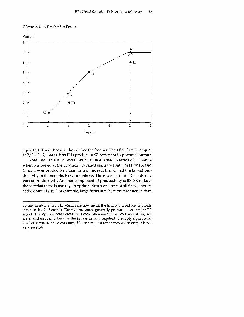
frontier. In figure 2.3 firms A, B, and C are used to construct the frontier,and the other two firms, D and E, lie below the frontier.4

The distance between the data point and the frontier determines the -1Xof the firm. For example, firm E in figure 2.3 could potentially increase itsoutput up to the frontier (at point A). Hence we define the TE of firm E asbeing equal to the ratio of what it is producing (6 kl) over what it couldpotentially produce (7 kl), given i Ls curren, level of inputs (5 laborers). Thusfor firm E, TE = 6/7 = 0.86, that is, it is producing 86 percent of its potenLialoutput.5 The TE of the frontier firms in figure 2.3 (firms A, B, and C) is

4. Standard production functions are usually fitted using regression methods.These regression methods fit a line through the cenier of the data, and hence nea-sure average practice. Frontier methods, by contrast, fit a surface over the data,and hence measure best practice

5 This measure of TE is called output-oriented, because it asks by how muchthe firm could increase its output given its level of Inputs. Alternatively, one can

Wlhy Should Regulators Be Interested in Efficiency? 15

Figure 2.3. A Production Frontier

Output

8

A7

6 E

5

4

3

2

0 1 2 3 4 5 6

Input

equal to 1. This is because they define the frontier The TE of firm D is equalto 2/3 = 0.67, that is, firm D is producing 67 percent of its potential output.

Note that firms A, B, and C are all fully efficient in terms of TE, whilewhen we looked at the productivity ratios earlier we saw that firms A andC had lower productivity than firm B. Indeed, firm C had the lowest pro-ductivity in the sample. How can this be? The reason is that TE is only onepart of productivity. Another component of productivity is SE. SE reflectsthe fact that there is usually an optimal firm size, and not all fiLrms operateat the optimal size. For example, large firms may be more productive than

defmne input-oriented TE, which asks how much the firm could reduce its inputsgiven its level of output The two measures generally produce quite similar TEscores. The input-oriented measure is most often used in network industries, likewater and electricity, because the firm is usually required to supply a particularlevel of service to the community. Hence a request for an mcrease in output is notvery sensible.

16 A Prinmer on Efficiency Measutrementfor Utilities iid Trnatsport Regtulators

small firms because they can have labor teams that specialize in particu-lar tasks.

To measure scale efficiency we must construct an additional frontier onfigure 2.3, namely, a constant returns to scale (CRS) frontier. This is a fron-tier that allows firms of any size to be benchmarked against each other, WIrexample, small firms can be benchmarked against big firms and vice versa.The frontier that we have already drawn in figu-re 2.3 is known as a vari -able returns to scale (VRS) frontier. This VRS frontier was constructed sothat small firms are benchmarked against small firms and big firms againsibig firms.

A VRS frontier and a CRS frontier are drawn in figure 2.4. In this simpleexample, the CRS frontier is simply equal to the line from the origin throughthe point defined by firm B. Firm B is chosen because it has the largestproductivity. The distance between each data point and the CRS frontier iscalled TECRS' This measure of efficiency will contain both TE and SE. Forexample, consider firm D in figure 2.4. It has TECRS = 2/3.33 = 0.6. The gap

Figure 2.4. CRS and VRS Productioni Frontiers

Output

8

/Z A7 CRS frontier

6 KE

5~~~~~~~~~VRS frontier

4

I C

0 1 2 3 4 5 6

Input

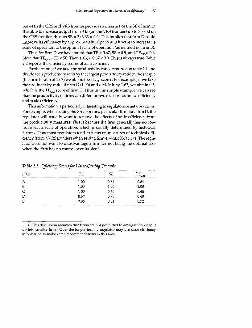
Why Should Regulators Be Interested in Efficieniczy? 17

between the CRS and VRS frontier provides a measure of the SE of firm D.It is able to increase output from 3 kl (on the VRS frontier) up to 3.33 kl onthe CRS frontier, thus its SE = 3/3.33 = 0.9. This implies that firm D couldimprove its efficiency by approximately 10 percent if it were to increase itsscale of operation to the optimal scale of operation (as defined by firm B).

Thus for firm D we have found that TE = 0.67, SE = 0.9, and TECRS = 0.6.Note that TECRs = TE x SE. That is, 0.6 = 0.67 x 0.9 This is always true. Table2.2 reports the efficiency scores of all five firms .

Furthermore, if we take the productivity ratios reported m table 2.1 anddivide each productivity ratio by the largest productivity ratio in the sample(the firm B ratio of 1.67) we obtain the TEcRs scores. For example, if we takethe productivity ratio of firm D (1.00) and divide it by 1.67, we obtain 0.6,which is the TEc,<s score of firm D. Thus in this simple example we can seethat the productivity of firms can differ for two reasons: technical efficiencyand scale efficiency.

This information is particularly interesting to regulators of network firms.For example, when setting the X-factor for a particular firm, say firm D, theregulator will usually want to remove the effects of scale efficiency fromthe productivity measures. This is because the firm generally has no con-trol over its scale of operation, which is usually determined by historicalfactors. Thus most regulators tend to focus on measures of technical effi-ciency (from a VRS frontier) when setting firm-specific X-factors. The regu-lator does not want to disadvantage a firm for not being the optimal sizewhen the firm has no control over its size.6

Table 2.2. Efficiency Scoresfor Water-Carting Exanmple

Firm TE SE TECRs

A 100 0 84 0.84B 1.00 1.00 1.00C 1 00 0.60 0.60D 0.67 0 90 0 60E 0.86 0.84 0.72

6. This discussion assumes that firms are not permitted to amalgamate or splitup into smaller firms Over the longer term, a regulator may use scale efficiencyinformation to make some recommendations in this area

18 A Primer o0? Efficiency Measuirenientfor Utilities anid Tranisport Reglilators

The discussion thus far has used a simple one-input, one-output cxample. If we consider the more general case of multiple-inputs and/ormultiple-outputs, we are required to measure productivity as the ratio ofan output index divided by an input index. The input index is generallydefined as a weighted sum of all inputs, and the output index is a weightedsum of all outputs.

TFP output indexinput index

The weights used in these indexes are usually cost shares in the inputindex and revenue shares in the output index, that is, we use price informa-hon. These price-based index number (PIN) methods are described in detailin the next chapter. Note that the index number formula most commonlyused in TFP calculations is the Tornqvist index (defined in chapter 3).

When we have multiple inputs and multiple outputs we find that TFPcan now differ between firms for four reasons:

o Technical efficiencyo Scale efficiencyo Input mix allocative efficiencyo Output mix allocative efficiency.

Input mix allocative efficiency relates to the notion that the firm is try-

ing to produce its output using the least-cost mix of inputs, given the inputprices the firm faces. For example, if the price of capital falls relative to theprice of labor, the firm may be able to reduce its costs by using less laborand more capital, for instance, by introducing a new computerized billingsystem.

Output mix allocative efficiency relates to the notion that the firm istrying to produce the optimal mix of outputs given the output prices thefirm face. For example, if the price of sewerage removal rises relative to theprice of water supply, one of the Indian water-carting firms we used in ourearlier example may be able to increase its revenues by delivering losswater and removing more sewerage without changing the amount of in-puts used.

When settmg firm-specific X-factors, a regulator will often want tc re-move these allocative efficiency factors from the performance comparisonsbetween firms. The regulator may wish to remove the input mix alloca tiveefficiency component because the capital intensity of network firms is of-ten largely determined by population density. Furthermore, the output mix

Wlhy Should Regulators Be Interested itn Efficiency7 19

allocative efficiency component is often removed because network firmsrarely have the ability to alter their output mix, for instance, a mix of largeand small customers.

Hence in setting the firm-specific part of the X-factors, regulators tendto focus primarily on measures of technical efficiency. This is not an abso-lute rule, but it is generally the case. Note also that this is a conservativeapproach. If the regulator included allocative efficiency (or scale efficiency)in the X-factor calculations, the X-factor could only rise.

The foregoing discussion relates to comparisons of the TFP of two ormore firms at one point in time. When we wish to compare the TFP of afirm or an industry over time, an additional factor can contribute to TFPgrowth, namely, technical change. Technical change can be represented byan upward shift in the production frontier over time. It could, for example,be the result of the development of new technology, such as new equip-ment for cleaning and re-lining old pipes in a water supply firm.

A number of authors refer to technical change as a frontier-shift and totechrucal efficiency change, that is, getting closer to the frontier, as catch-up.

To summarize, TFP growth over time could be the result of five factorsas follows:

* Technical change (frontier shift)* Technical efficiency change (catch-up)* Scale efficiency change* Input mix allocative efficiency change* Output mix allocative efficiency change.

When setting X-factors, a regulator generally wants to ask the frontierfirms to achieve an annual productivity improvement equal to the histori-cal level of technical change (frontier shift), and wishes to ask the ineffi-cient firms (those below the frontier) to achieve this plus some technicalefficiency improvement (catch-up).

In most cases the regulator will use price-based TFP indexes to measureTFP change in the industry over the last 5 or 10 years, and then use this TFPchange measure as an estimate of the likely future rate of technical changem the industry. This is generally a reasonable measure, but this is not al-ways the case. For example, during a period following a change in regula-tory structure, the new incentives may have encouraged a number ofinefficient firms to catch up to the better firms. In this case the industry-level TFP change measure could be 3 percent per year, with 1 percent re-sulting from technical efficiency change (catch-up) and 2 percent fromtechnical change (frontier shift). Now if the regulator uses the 3 percent

20 A Primer on Efficiency Measurementtfor Utilittie anid Transport Regitlators

measure as a measure of potential technical change, the frontier firms willbe asked to do too much.

This brings us to an important point: price-based TFI' index numbersmeasure TFP, but they cannot be used to decompose TFP into ihe foregoingcomponents. You need an estimate of the technology (the production fron-tier) to be able to decompose TFP into componeni-ts. This is one of the maindisadvantages of TFP index numbers; however, index numbers do havethe advantage that they only require data on two observations, for instance,two firms, while frontier methods require data on a large number of firms.

Two main approaches are used to construct production frontiers, OEAand SFA. For both methods we require data on the input and output quan-tities used by a sample of firms. We then fit a frontier over the top of thesedata points and measure technical inefficiency as the distance between eachdata pomt and the estimated frontier. DEA uses linear programming meih-ods to construct the frontier, while SFA uses methods similar to regressionmethods, but more complex.

The two methods have various advantages and disadvantages. SFA hasthe advantage that it attempts to account for the effects of data noise (daLaerrors, omitted variables, and so on), while DEA assumes the data are 'reeof noise. SFA has the second advantage that you can use standard statisti-cal tests such as t-tests to test the significance of variables included in ;hemodel, while DEA does not allow this. However, DEA has the advaniagethat you do not need to specify a functional form for the produc.ion fron-tier, while in SFA you must select a functional form, for example, logarith,l-mic. Another advantage of DEA is that it is easier to calculate using availablesoftware than SFA.

Overall, both methods have their merits. If possible, using both m^th-ods as a sensitivity test is wise, and generally they should produce similarresults.7 In regulation, DEA has been the rnore popular method, probablybecause DEA methods are easy to draw on diagrams, easy to calculate, anduntil recently SFA could not accommodate multiple outputs.'

7 For an example of a study that applied a number of methods to one datasetsee Carrington, Coelli, and Groom (2002), who applied DEA, SFA and corrc Ledordinary least squares to data on Ausiralian and U.S. gas distributors for the pur-pose of setting price caps.

8. SFA methods can now easily accommodate multiple outputs using a mul.i-output production finction known as a distance function.

Why Should Regulators Be Interested in Efficiency2 21

This chapter has introduced a good deal of terminology. To help sum-marize this information we provide two summaries. Box 2.1 provided in-formal definitions of some of the performance measurement terminologycommonly used in regulatory debates, such as efficiency and technicalchange, and can be used for reference. Table 2.3 compares the key charac-teristics of the three main performance measurement methods: price-basedindex number (PIN), SFA, and DEA.

Summing Up

In this chapter we described an example of a situation where a regulatorwishes to set price caps for electricity distribution firms and discussed thepossible pitfalls of using simple performance measures. We then outlinedthe types of information that can be derived from the use of more sophisti-cated performance measurement methods. In particular, we discussed howproductivity differences between firms could be decomposed into variouscomponents, including technical efficiency, scale efficiency, and allocativeefficiency, and how productivity changes over time can be decomposedinto technical change (frontier shift), technical efficiency change (catch-up),scale efficiency change, and allocative efficiency change.

In many instances a regulator can benefit from having access to thisricher information. For example, consider the case where a regulator hasinformation on productivity differences between firms, but has no infor-mation on the contribution of scale efficiency in these differences There isa danger that the regulator could set unachievable productivity targets onthe small firms if they face scale diseconomies.

Alternatively, consider the case where a regulator has obtamed a mea-sure of industry productivity growth over the last five years of 5 percentper year, but has no information on the contribution of technical change(frontier shift) in this figure. If part of the productivity growth, say 2 per-cent, was due to technical efficiency change (catch-up) derived from achange in regulatory regime, and hence only 3 percent was due to technicalchange (frontier shift), then a request for 5 percent productivity growthover the next five years may be too high if little scope remains for continu-ing catch-up over the next five years.'

9 For a change m regulatory regime to induce this type of catch-up effect is notunusual. For example, consider the case of the U.K. electricity industry, whichachieved substantial growth m productivity in the period following the change toprice cap regulation.

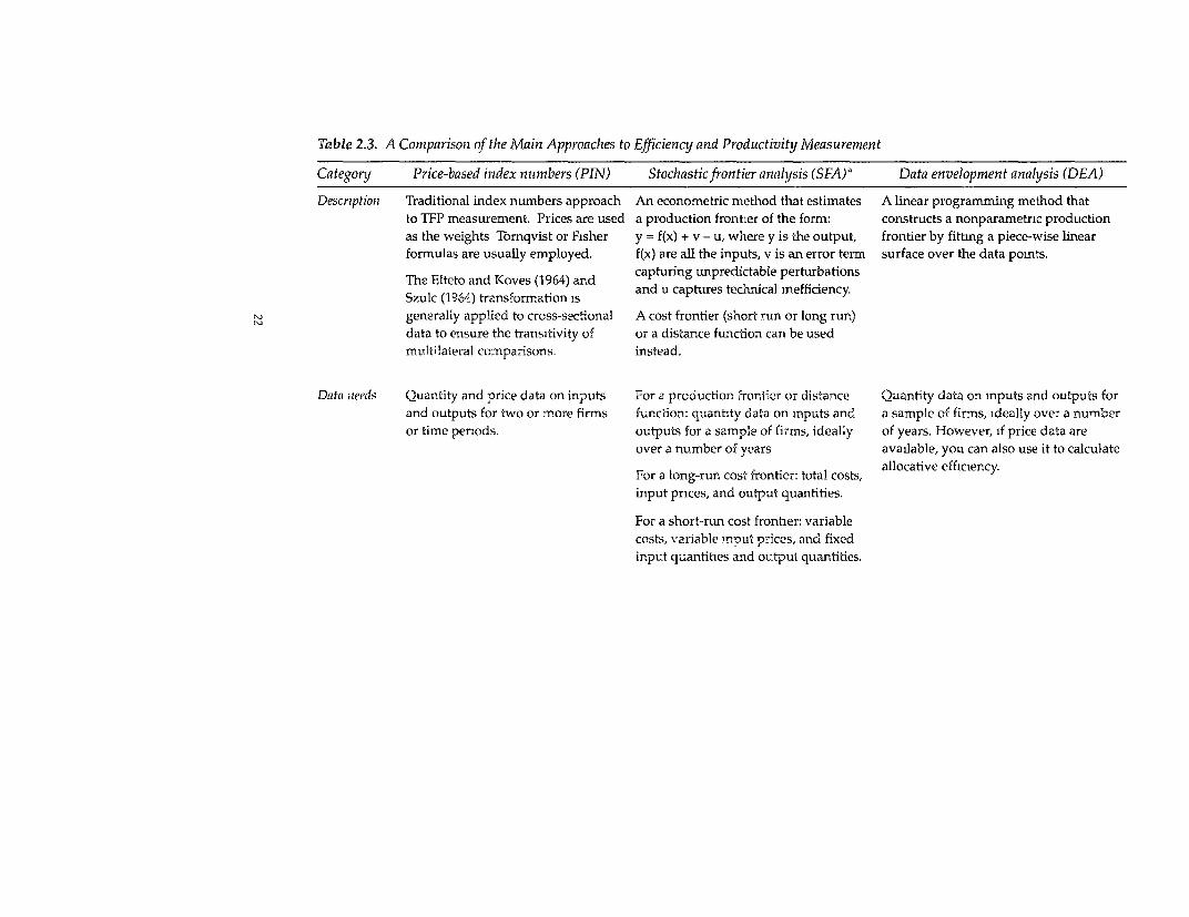
Table 2.3. A Comparison of the Main Approaches to Efficiency and Productivity Measurement

Category Price-based index nuimbers (PIN) Stochasticfrontier analysis (SFA)' Data envelopment analysis (DEA)

Descriptionz Traditional index numbers approach An econometric method that estimates A linear programming method that

to TFP measurement. Prices are used a production fronter of the form: constructs a nonparametric production

as the weights Tornqvist or Fisher y = f(x) + v - u, where y is the output, frontier by fitting a piece-wise linear

formulas are usually employed. f(x) are all the inputs, v is an error term surface over the data points.

The Elteto and K(oves (1964) and capturing unpredictable perturbationsSzulc (1964) transformation is and u captures technical mefficiency.

generally applied to cross-sectional A cost frontier (short run or long run)

data to ensure the transitivity of or a distance function can be usedmultilateral comparisons. instead.

Data needs Quantity and price data on inputs For a proauction 2rontier or distance Quantity data on inputs and outputs for

and outputs for two or more firms f-unction: quantity data on mputs and a sample of firms, ideally over a number

or time penods. outputs for a sample of firms, ideally of years. However, if price data are

over a number of years available, you can also use it to calculateallocative efficiency.

For a long-run cost frontier: total costs,input prices, and output quantities.

For a short-run cost frontier: variablecosts, variable input prices, and fixedinput quantities and outpui quantiiies.

Advantages Can do a study with only two Attempts to account for noise. Identifies a set of peer firms (efficientobservations firms with similar input and outputEnvironmental variables are easier mixes) for each inefficient firm.Is reproducible and transparent. to deal with.

Captures allocative efficiency. Allows for the conduct of traditional Can easily handle multiple outputs.stafistical tests of hypotheses. Does not assume a functional formEasier to identify outijers. for the frontier or a distributional

form for the inefficiency error term.Cost frontier and distance function candeal with multiple outputs.

Drawbacks Need price information. The decomposition of the error term May be influenced by noise.

Cannot decompose TFP measure into noise and efficiency components Traditional hypothesis tests are notmay be affected by the particular .bdistributional forms specified and by pthe related assumption that error skew- Requires large sample size for robustness is an indication of inefficiency estimates, which may not be available

Requwres large sample size for robust early on m the life of a regulatorestimates, which may not be availableearly on in the life of a regulator

a Ordinary least squares (OLS) estimation of a frontier can be viewed as a special case of SFA, where one assumes that there is no inefficiency CorrectedOLS estimation, where the OLS intercept is shifted so that the frontier envelopes all data points, is also a special case of SFA where one assumes that there isno noise

b. This drawback may be limited using bootstrapping techniques as proposed by SLmar and Wilson (2000)

24 A Primer on Efficiency Measurement for Utilities and Transport Regulators

These two examples illustrate how the use of sophisticated performanccmeasurement methods can help regulators make better-informed decisions.However, these sophisticated methods require access to good quality data.In the following two chapters we will assume that wc have access to goodquality data and outline how to measure and decompose productivitychange using a number of alternative approaches. In later chapters we willrelax the good data assumption and discuss some of the available options.

3Some TFP Measurementand Decomposition Methods

We begin this chapter by noting that it involves much technical discussionof how to measure TFP and how to decompose these TFP measures intocomponents that are of interest to regulators. This chapter assumes that wehave access to good quality data, an assumption that is relaxed in laterchapters.

As noted in chapter 2, the definition of TFP is intuitively quite simple Ittells the regulator how much output is achieved with each unit of input,which would seem to be a reasonable performance indicator for most situ-ations a regulator has to face. In other words, it is equal to the ratio ofoutput over input, and when there is only one output (Y) and one input(XI), it boils down to the following expression:

TFP = Y,/X,. (3 1)

This formula is, however, too simple in practice, because most opera-tors tend to rely on a combination of inputs, for instance, labor, capital, andothers, that can have varying relative importance across firms. Moreover,many regulated industries offer multiple outputs as well. For instance, anairport, port, or rail operator will often cater to both freight and passengers.A water company can produce water, distribute it, collect raw sewerage,and treat the sewerage, which are all separate products. Telecommunica-tions operators often offer both local and long distance services and manyfixed operators are diversifying into mobile telephony. Moreover, the latesttrend in the sector is to have multi-utility operators. Many electricity

25

26 A Primer on Efficiency Measuremenitfor Utilites a,ad Tranisport Regulators

operators are crossing over to telecommunications and the main interna-tional actors in the water sector are following. This suggests that a reason-able measure of TFP generally needs to take into account M outputs and i(

inputs, where M and K are usually both larger than one.As noted in chapter 2, a TFP index is generally constructed as the ratio

of an output index to an input index. For example, we could use a linearweighting function to define a TFP index as

TFP = 7 an,Ym h/,b Xk, (3.2)

where am and bk are weights that reflect the relative importance of the vari-ous inputs and outputs.

Two questions follow directly from equation (3.2). First, how do we se-lect the values for the weights? Second, is a linear function appropriate orshould we choose another mathematical form? 'Ilhe issue of the approp--i-ate mathematical form to choose will be dealt with later in this chapter. Atthis point we will focus on the weights issue. There are two natural choices:market prices and shadow prices.

Market prices are the prices that people must pay for the goods or se:--vices. For example, consider the case of a water supply firm. Some relevan.input prices could be the wage rate per hour for labor and the rental priceper hour for a computer. Some relevant output prices could be the priceper liter for water supply and the price per day of sewerage connection.

Shadow prices, by contrast, are derived from the shape of the underly-ing production technology (or frontier), and are usually expressed in ratioform. For example, the ratio of the shadow price of labor tc the shadowprice of computers would reflect the degree to which an hour of labor canbe substituted with some quantity of computer hours (wit'h output levelsheld constant). In economics jargon this reflects the marginal rate of t'echni-cal substitution between the inputs. Similarly, the ratio of the shadow priceof water supply to the shadow price of sewerage services would reflect .hedegree to which a liter of water supply can be substituted with some qua-tity of sewerage services (with input levels held constant). in economicsjargon this reflects the marginal rate of technical transformatiLon be'nwv: .i

the outputs.Under conditions of perfect competition, shadow prices and market.

prices will be equal. If they are not equal, we say that a certain amount ofinput mix or output mix allocative inefficiency exists. h-lowever, we need to

Some TFP Measuiremenit and Decomposition Methods 27

be careful here, because if the market prices are in some way distorted, forexample, because of a regulatory or political intervention, the issue ofallocative inefficiency is less clear.

The methods used to measure TFP can be divided into two groups ac-cording to the types of prices employed, that is, market or shadow prices.In chapter 2 we introduced three groups of methods (table 2.3):

* Price-based index numbers* Stochastic frontier analysis* Data envelopment analysis.

Essentially, PIN methods use market prices, while SFA and DEA meth-ods involve the estimation of a production technology (frontier), and hencethe use of shadow prices derived from the shape of the estimated frontier.

In the remainder of this chapter we provide a detailed description ofhow to use these methods to measure TFP growth. We also describe howyou can use the frontier methods (SFA and DEA) to decompose the mea-sured TFP growth into components that are of interest to regulators.

Price-Based Index Numbers

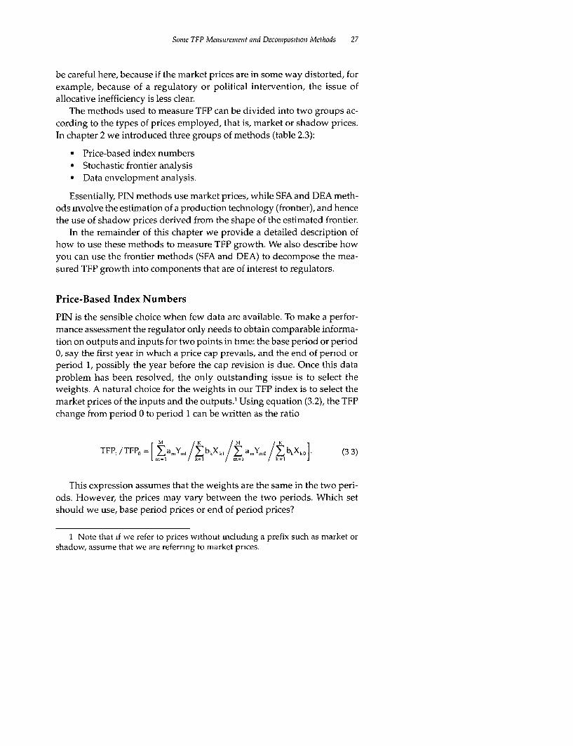
PIN is the sensible choice when few data are available. To make a perfor-mance assessment the regulator only needs to obtain comparable informa-tion on outputs and inputs for two points in time: the base period or period0, say the first year in which a price cap prevails, and the end of period orperiod 1, possibly the year before the cap revision is due. Once this dataproblem has been resolved, the only outstanding issue is to select theweights. A natural choice for the weights in our TFP index is to select themarket prices of the inputs and the outputs.1 Using equation (3.2), the TFPchange from period 0 to period 1 can be written as the ratio

[ M K M K

TFP1 / TFP, = [amY,l /bkXkl Y a. Y Y bkXkoj] (3 3)ml k=1 1/ m=l k=1l

This expression assumes that the weights are the same in the two peri-ods. However, the prices may vary between the two periods. Which setshould we use, base period prices or end of period prices?

1 Note that if we refer to prices without including a prefix such as market orshadow, assume that we are referring to market prices.

28 A Priner on Efficenecy Measurementefo, Ublitiet; nad Tr'ilsport Regulators

Using the base period prices yields a TF? index, which is the ratio of aLaspeyres output quantity index to a Laspeyres input quantity index. Us-ing period 1 prices (assuming that this is the end or period) yields a Paascheindex. Many regulators would see this choice as arbitrary and prefer to relyon the geometric mean of these two indexes, which is known as the Fisherindex.2 A popular alternative in recent publications on TFI' measures inprivatized industries, which provides nearly identical results, is theTornqvist index, which implies an underlying tranislog technology.

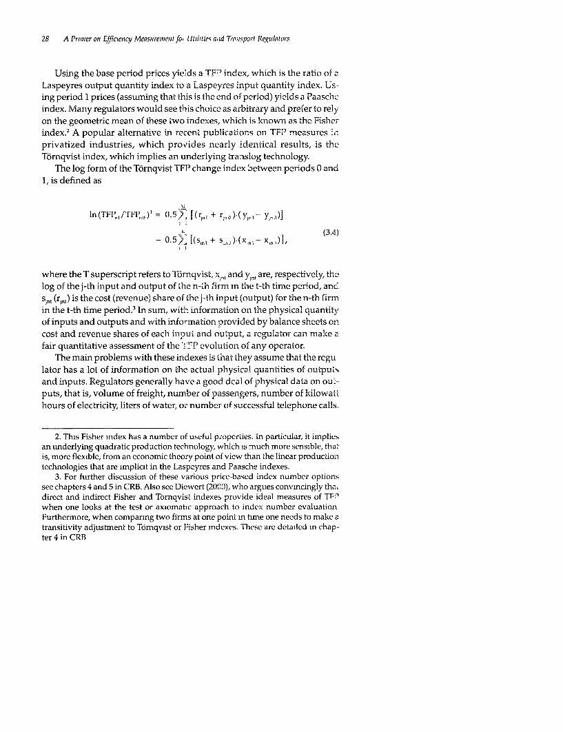
The log form of the Tornqvist TFP change index between periods 0 and1, is defined as

V

ln(TFP,,/TFP,,) 1= 0.5>' [(r,n, + r,e ),(y,- YInIO

I I

0.5 E [(S., + s,,, ).(x,- x,,)l, )3.4

where the T superscript refers to Tdrnqvist, x,,, and Yint are, respectively, thelog of the j-th input and output of the n-ih firm in the t-th time period, ancdsjnl (rl) is the cost (revenue) share of the j-th input (output) for the n-th firmin the t-th time period. 3 In sum, with information on the physical quantityof inputs and outputs and with information provided by balance sheets oncost and revenue shares of each input and output, a regulator can malke afair quantitative assessment of the T7P evolution of any operator.

The main problems with these indexes is that they assume that the regulator has a lot of information on the actual physical quantities of outpuisand inputs. Regulators generally have a good dcal of physical data on ou.-puts, that is, volume of freight, number of passengers, number of kilowa. hours of electricity, liters of water, or number of successful telephone calls.

2. This Fisher mdex has a number of useful p;operiies. In particular, it impliesan underlying quadratic production technology, which is mnuch more sensible, tha is, more flexible, from an economic theory point of view than the linear productiorntechnologies that are implicit in the Laspeyres and Paasche indexes.

3. For further discussion of these various price-based index number optionssee chapters 4 and 5 in CRB. Also see Diewert (2000), who argues convmcingly thc.direct and indirect Fisher and Tbrnqvisi indexes provide ideal measures of TF Iwhen one looks at the test or axiomatic approach to index number evaluationFurthermore, when comparing two firms at one point in time one needs to make .transitivity adjustment to T6mqvist or Fisher mdexes. These are detailed in chap-ter 4 in CRB

Sonie TFP Measurement and Deconiposition Methods 29

They generally have much less physical data on inputs. Indeed, unless theyare required to provide the information, operators will seldom volunteerthe physical measure of inputs such as energy consumption. This limiteddata on quantity pushes the regulator to use as much as possible the in-formation available in balance sheets, that is, cost and revenue data fromannual reports. This can be frustrating, as little detailed breakdown of thisinformation is generally available unless the regulator has managed toimpose strict regulatory accounting rules on the operators. In this respectthe Office of Water Services in the United Kingdom is a leader in the field(see www.open gov.uk/ofwat).

One solution in that type of situation is to rely on an mdirect TFP index.This indirect index is defined by deflating total revenue and total costs bysuitable price indexes to obtain quantity indexes That is, because price xquantity = value, then quantity = value/price. One can then define TFP asthe ratio of deflated revenue over deflated cost.4 This is also an approxima-tion, because often the price indexes that are used for deflating are imper-fect, as discussed later. They are probably compiled for the industry by acentral statistical agency. Recognizing these constramts is crucial, becausethey may introduce biases into the TFP measurements.

To see how these biases could occur in practice, consider the case of arailways performance study The best input price index available might bethat defined for public transport mdustries in general, while the outputprice index may be defined for the rail mdustry alone. These price indexeswould most likely be Laspeyres indexes, that is, based on base periodweights, and would also be calculated using quantity weights for the wholeindustry. Hence if the input mix and/or output mix of a particular firmdiffers substantially from the average mixes in the industry, for example, ifa firm uses a lower proportion of labor to capital or provides a higher pro-portion of freight to passenger services, the deflated revenue and/or costfigures for this firm may not provide a reasonable approximation to therequired quantity indexes. Thus the resulting TFP index for this firm maybe misleading.

How misleading can this be? Imagine a case where the ratio of passen-ger to freight services is 4 to 1 in the industry in terms of revenue, but firm

4. Once again, the form of the price index formula used (Laspeyres, Paasche,Thinqvist, or Fisher) will imply a particular functional form for the underlyingproduction technology. Laspeyres and Paasche will imply restrictive first-orderforms, while Tmrnqvist and Fisher imply more flexible second-order functionalforms

30 A Primer on Efficiency Measurementfor Utilities anzd Transport Regulators

A has a ratio of 1 to 4 (we assume all firms face the same prices). If the pric2of passenger services increases by 10 percent between two periods whilethe other prices and all quantities remain constant, the output price indexfor the industry will increase by 8 percent, while the true price index firm Afaces will only increase by 2 percent. However, the revenue of firm A, whichincreases by 2 percent, will be deflated by the industry price index, whichincreases by 8 percent, which will suggest that the real output of firm A hasfallen, when in reality it has not.5

In sum, the PINs can be useful to many regtilaiors with only limiteddatabases, but as with any index, unders'tanding the instrument's limitations is a requirement for ensuring the credibility of its regulatory uses. Anecessary condition for its effective use is a good understanding of whateach price indicator hides and the extent to which average price applies ofdoes not apply to any individual operator.

PIN methods have the advantage that they can be used when you onlyhave access to data on one firm or a few firms, or you only have access toindustry-level data; however, they have the disadvantage that you canno.use PIN methods to decompose TFP change into components, such as tech-nical change (frontier shift) and technical efficiency change (catch-up). Inthe following sections we assume that we have access to panel data on anumber of firms, that is, we have data on N firms over T time pseriods, forexample, we could have annual data on N = 40 firms over T = 8 years.Given access to this type of data, we can use frontier methods such as SPFA.and DEA to measure and decompose TFP growth.

iroduction lFruneiers, Singl C: e : CEse

For the sake of simplicity, we focus first on the standard single output pro-duction process, and leave the discussion of the multiple output case forlater. This discussion is quite relevant in practice, as many regulators t-en6to treat the firms they monitor as single output producers and rely on .

5. These types of issues are also important to keep in mind as we discuss pro-duction and cost frontier approaches to TFP measurement, because our quantitydata often come in the form of deflated value measures. In many cases the priceswe use may be questionable. First, they may be measured with error. Second, the.may be measured well, but some prices may be distorted by regulatory and othcrfactors, for example, a government-owr:ed utility might set electricity prices belowcost. Third, the market prices may be measured well, but they may not reflec.society's priorities, for instance, this may be revealed in divergences between themarket price and shadow price of labor in government-owned firms where tiegovernment and society put a value on high employment levels.

Some TFP Measuremenit and Decomposition Methods 31

constant price valuation of the operator's revenue as an approximation ofthis output.

The TFP change (TFPC) measures derived from a production frontiercan be decomposed into three components: technical efficiency change(TEC), technical change (TC), and scale efficiency change (SEC). This de-composition is multiplicative, that is,

TFPC = TEC x TC x SEC

Note that allocative efficiency does not appear in this decomposition.This is because the TFP measures derived from production frontiers do notinclude this factor; however, allocative efficiency does come into play whenwe consider cost frontiers.

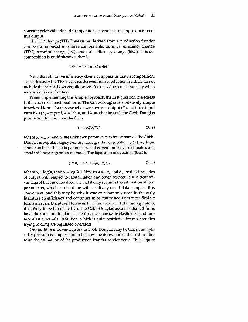
When implementing this simple approach, the first question to addressis the choice of functional form. The Cobb-Douglas is a relatively simplefunctional form. For the case when we have one output (Y) and three inputvariables (X, = capital, X2 = labor, and X3 = other inputs), the Cobb-Douglasproduction function has the form

Y = a0X, X2`X3,` (3.4a)

where ao, 1x2, and 01 are unknown parameters to be estimated. The Cobb-Douglas is popular largely because the logarithm of equation (3.4a) producesa function that is linear in parameters, and is therefore easy to estimate usingstandard lnear regression methods. The logarithm of equation (3.4a) is

y = (to + A + (X2X2+ O3x3, (3 4b)

where a, = log(a,) and x, = log(X,). Note that otL, (X2 and a3 are the elasticitiesof output with respect to capital, labor, and other, respectively. A clear ad-vantage of this functional form is that it only requires the estimation of fourparameters, which can be done with relatively small data samples. It isconvenient, and this may be why it was so commonly used in the earlyliterature on efficiency and continues to be contrasted with more flexibleforms in recent literature. However, from the viewpoint of most regulators,it is likely to be too restrictive. The Cobb-Douglas assumes that all firmshave the same production elasticities, the same scale elasticities, and uni-tary elasticities of substitution, which is quite restrictive for most studiestrying to compare regulated operators.

One additional advantage of the Cobb-Douglas may be that its analyti-cal expression is simple enough to allow the derivation of the cost frontierfrom the estimation of the production frontier or vice versa. This is quite

32 A Primer on Efficency Measurementfiir Utilities onid Tatusport Regulators

useful when a regulator can only rely on total cost data from balance sheets.It is, however, quite problematic conceptually, as most of the analytical workunderlying the duality between production and cost frontiers assumes per-fectly competitive markets, which is rarely the norm among regulated in-dustries. They are regulated because they are not strictly competitive.'Because of this, it is often safer to use a production frontier if you haveaccess to suitable data.

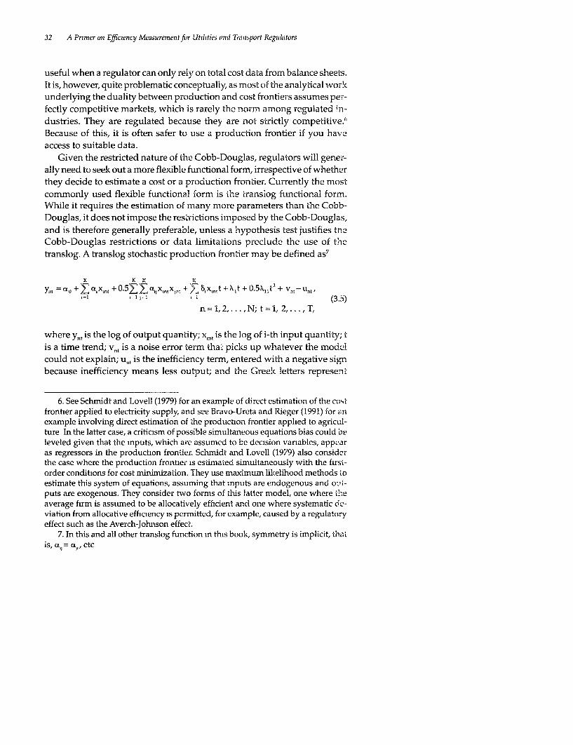
Given the restricted nature of the Cobb-Douglas, regulators will gener-ally need to seek out a more flexible functional form, irrespective of whetherthey decide to estimate a cost or a production frontier. Currently the mostcommonly used flexible functional form is the -ranslog functional form.While it requires the estimation of many more parameters than the Cobb-Douglas, it does not impose the restrictions imposed by the Cobb-Douglas,and is therefore generally preferable, unless a hypoothesis test justifies tneCobb-Douglas restrictions or data limitations preclude the use of thetranslog. A translog stochastic production frontier may be defined as7

K K K K

Yn1 °=0 +E(XlXmt +0 5EEal,X +7 8x,X. \,t + O.5X,1 t2 + V-,-I I 1 (3.5)

n=1,2,...,N; t=l, 2,...,T,

where Yn, is the log of output quantity; x,,, is the log of i-th input quantity; tis a time trend; vnt is a noise error term tha, picks up whatever the modelcould not explain; unl is the inefficiency term, entered with a negative signbecause inefficiency means less output; and th-e Greek letters represent

6. See Schmidt and Lovell (1979) for an example of direct estimation of the costfrontier applied to electricity supply, and see Bravo-Ureta and Rieger (1991) for anexample involving direct estimation of the produchon frontier applied to agricul-ture In the latter case, a criticism of possible simultaneous equations bias could beleveled given that the mputs, which are assumcd to be decision variables, appoaras regressors in the production frontier. Schmidt and Lovell (1979) also considcrthe case where the production frontier is estimated simultaneously with the first-order conditions for cost minimization. They use maximum-n likelihood methods Loestimate this system of equations, assuming that mputs are endogenous and oui-puts are exogenous. They consider two forms of this latter model, one where theaverage ftrm is assumed to be allocatively efficient and one where systematic cc-viation from allocative efficiency is permitted, for example, caused by a regulatoryeffect such as the Averch-Johnson effeci.

7. In this and all other translog function m this book, symmetry is implicit, thaiis, a,~ = Up etc

Some TFP Measurenient and Decomposition Methods 33

unknown parameters to be estimated.8 The subscripts n and t index firmand time period, respectively. As is also quite comrmon, in this model wehave used a time trend, t, to approximate technical change. While otherpossibilities exist, such as the use of annual dummy variables, the timetrend approach is the most often used.9

A useful trick practitioners use that deserves consideration by most regu-lators is transforming the data so as to allow direct interpretation of the first-order translog parameters (the a,s) as the elasticities evaluated at the samplemeans.'° This is done by ensuring that the arithmetic sample averages of thelogged variables are 0, which is equivalent to setting the geometric means ofthe original (unlogged) data equal to 1. Essentially it consists of dividingevery series by its geometric average. This wiRl not change the results ob-tained, but is simply a convenient change in units of measurement.

The next stage is the actual calculation of the TFPC for each firm betweenany two time periods using estimates of the production frontier. FollowingOrea (2002),"i the log of the TFPC between period t = 0 and t = 1, for then-th firm can be defined to being equal to

In (TFP,, / TFPnO) = In (TE., /TEnl ) + 0.5 [(dy, 0/t) + (ay, /at)]K (3 6)

+ 0.5L [(SFoekno + SFn( ek36) H Xk1 Xk.0k=1

8 Those more statistically inclined shoudd note that the most common as-sumptions are that the error terms, vn, and u,,, could take many different possiblestructures The first is symmetrically distributed while the second is one-sidedGenerally they are assumed to be independently and identically distributed asN(0, u(2) and I N(0, u,:) random variables, respectively (see chapters 8 and 9 inCRB for further discussion)

9 In addition to this general specification, there is the need to ensure that thesum of the weights in the TFP measure adds up to 1. If the production elasticitiesfrom the estimated production frontier do not add up to 1, the literature usuallypicks either one of the followng two choices The first is to impose constant re-turns to scale on the production technology, but this will generally not be satisfac-tory in regulated industries, which are often considered to be natural monopolieswith clear economies of scale. The second is to assume variable returns to scale andensure that an appropriate scale efficiency change measure is included m the finalTFP calculations, as suggested In Balk (1999), Kumbhakar and Lovell (2000), andOrea (2002) Most regulators will generally favor this approach.

10 If you do use scaled data to estimate the frontier, then you must be sure to usescaled data to calculate TFP, and so on, otherwise you will obtain incorrect results.

11. The two main approaches to TFP decomposition are the total differentialapproach (see, for example, Bauer 1990; Kumbhakar and Lovell 2000) and the index

34 A Primer on Efficiency Measurement for Utilities a1nd Tranzsport Regulotors

where the three terms on the right-aand-side of equation (3.6) are the TB'C,TC, and SEC terms, respectively. Tlhe technical efficiency measure, TEDt, isthe technical efficiency prediction of the n-th firm in the t-th time periodobtained from equation (3.5).i2 The technical change measure is the meanof the technical change measures evaluated at the period 0 and period 1data points, and can also be derived directly frorn the coefficients estimatedfor equation (3.5). The change in scale efficiency requires calculating theproduction elasticities from the parameters estimated for equation (3.5),'that is, you must calculate

e, = ay., /ax,,< - a,; -1- Tc x,8 + o,t (3.7). 1

for each input at each data point, and also calculate the scale factors

SFnt = (e.j- 1)/en, at each data point, where e,Z = Z,c is the standard returnsk I

to scale elasticity.'4

The TC measure requires calculating the partial derivative with respectto time at each data point. For firm n in period t this is

ayn1/at=XI+ )il t+ >7 xknt (3.8)

number approach (see, for example, Caves, Christensen, and Diewert 1982a,b; Crea2002), whuch exploits the translog identity. Tne two approaches result in almostidentical formulas, the only differences being that the latter approach evaluaiesderivatives at both data points, while the first method chooses just one data pointfor derivative evaluation. Diewert (2000) argues in favor of the index number ap-proach, because the total differential approach is an approxumation to a continu-ous time measure, which can take many values. Thus in this book we use the indexnumber approach, however, we do note that in most cases the two approaches willprovide quite similar estimates.

12. Analytically, the TE is equal to the conditional expeciation of exp(-un,), giventhe value of (v,j- unt). These measures are routinely reported by the statistical pack-ages available to assess efficiency, such as the FRON'TIER program by Coelli (1996b).TIus software can be downloaded from www.uq.edu.au/economncs/staff/coelli.htmn.

13. To be precise, the SEC measures derived from SFA frontlers in this book arenot pure measures of scale efficiency change. First, it is possible that the measuresobtained may also include the effects of scale-biased technical change, if this hasoccurred; however, this distinction is not something that regulators should be greatlyconcerned about. Second, as stated by Orea (2092 p 12), this term "evaluates thecontribution of non-constant returns to scale on productivity growth when firmsmove along the distance function changing their inputs levels over time."

14 With constant returns to scale, c, will equal 1, and hence the scale term Liequation (3 6) will be equal to 0, as required.

Some TFP Measurement and Decomposition Methods 35

Keep in mind also that the TFP index in equation (3.6) uses shadowprices, which are derived from the frontier, instead of market prices. If theregulator has access to input price data, it can also calculate the TornqvistTFP change index. For the single output case this is

K

ln(TFP., /TFPn.) =(ynl-y.) -0 5Z (Sk1+ SknO) (Xkni Xk0), (3 9)k=i

where s,, is the cost share of the k-th input of the n-th firm in the t-th period.Why should a regulator care about this calculation? Because any differ-

ence between the TFPC calculated from equations (3.6) and (3.9) must bedue to allocative efficiency change (AEC). In fact, we can show that AEC isas follows: 15

K

AEC = 0.5 E {[(ek.1 /e. 1 - skn1 ) + (eko, /e. 0 - skno)] (xknl - xk0)}. (3.10)k=1

This shows that the relative importance of distortions m the inputs mixcan help explain TFP changes, and their relative importance may be a sourceof concern that the regulator may not be able to do much about. Indeed,allocative efficiency changes may result from distortions in factor marketsnot really under the control of the operator. Limited access to capital mar-kets and national agreements with unions unrelated to the operator's spe-cialized employment needs are two common examples of sources ofallocative inefficiency for which the operator should not necessarily beblamed. Understandmg that this is the case is a matter of fairness. Chapter4 provides a detailed description of the application of these productionfrontier and Tornqvist methods to sample data.

15. Thus result will be exact when there is no noise in the model, that is, whenwe have a deterministic frontier. The expression in equation (3.10) has a nice intui-tive interpretation. Essentially it shows that the TFPC index that we constructed inequation (3.6), is equivalent to a Tornqvist mdex that uses shadow prices mstead ofmarket prices to calculate the input share weights. These shadow shares are equalto the production elasticities deflated by the retuins to scale elasticity. This defla-tion ensures that the shares sum to 1 as required. Thus the AEC measure in equa-tion (3.10) wllE pick up the effects of any convergence or divergence in the differencesbetween shadow prices and market prices, which may be due to regulatory andother change If shadow prices equal market prices m both periods, this term willclearly be equal to 0. Furthermore, if shadow prices and market prices do not changebetween periods, the term will also be 0.

36 A Primer on Efficiency Measurementfor Utilities anid Teaaspod Regulators

This quick introduction to the main concepts that regulators are likely

to come across in the literature would not be complete without some brie.-comments on a few of the simplest, and yet common, hypothesis tests regu-

lators will want to care about. Generally, testing for Cobb-Douglas versus

translog is not a bad idea, as is testing for neutral versus non-neutral tec7h-

nical change in any model aimed at measuring efficiency in a regulatedindustry for which few data are available. If one of 'Lhese sets of restrictions

holds, fewer parameters have to be estimated and the statistical results can

be more reliable with the same database size.These types of tests are essentially based on likelihood ratio tests, whic'n

compare the likelihood function value of each model, for instance, does thetranslog model do a significantly better job olf explaining variation in thesample data relative to the Cobb-Douglas function? They are quite rou-

tinely carried out in the literature to test these kinds of simple assumptionsand are quite simple to implement. For instance, to test for neutral techni-

cal change in a production frontier with K inputs tlhe steps are as follows:

1. Estimate the standard, unrestricted translog model and note the log-

likelihood function (LLF) value of this unrestricted model (LLFL).

2. Estimate the restricted model, where th-e IK x,t variables, which wouldimply a non-neutral technical change, are omitted, and note the re-

stricted LLF value (LLFR).3. Calculate the likelihood ratio test value, which is two times the dif-

ference between these two LLF values.4. Reject the null hypothesis of neutral technical change if the test value

exceeds the critical value, obtained from statistical tables. The likeii-hood ratio test statistic has a chi-square distribution, witlh degrees offreedom equal to the number of restrictions, in this case (.16

Cost 7Frontiers, SingRe Output CQse

Cost frontiers are commonly used, simply because cost data seem to be

much easier to come by. Ignoring tlhe significant conceptual issues raisedby cost functions in noncompetitive sectors, the main challenge for most

16. The procedure for the Cobb-Douglas versus translog test is similar. In thiscase the restricted model (the Cobb-Douglas) will only contain the first-order termsand the number of restrictions will be larger-!C(K + 1)/2-if a time trend is in-cluded. Furthermore, looking at efficiency scores and ranks before and after im-

posing restrictions is always wise to see if the imposition of restrictions has a bigeffect.

Some TFP Measurement and Decomposition Methods 37

regulators in developing countries without a strong tradition of good ac-counting standards is to make sure that the data mean something. Thedata must be comparable and consistent over time, and the definitions ofthe various cost concepts must be what most accountants would expectthem to be. This is not always easy to achieve in developing countrieswhere manipulating accounting data for tax reasons continues to be quitewidespread.

If and when these data are available, the most common functional formfound in the literature is a translog cost function, which essentially has costas a function of input prices and the production level. As for the produc-tion frontier, technical change is easy to incorporate, and this is often donewhen long enough time series are available to track down this change. Atypical translog cost function estimated in the utilities or transport sectortakes the following form:

K K K

= + E a,w,,,+ + 0 5 (Y., + P31y.t + 0.5 PI,Yn1=1 1~~~=1 j=iK K ~~~~~~'1 ~ Jt Vt n,(3 11)

E 1Wt Ynt +Y E w,mt + 41 yntt + I,t + 0 5X11t2+v,,+ u,

where Cnt is the log of total cost, Ynt is the log of output quantity, wnt is thelog of i-th input price, t is a time trend that is included as a proxy for tech-nical change, vnt is a noise error term, u,t is the cost inefficiency term, andthe Greek letters represent unknown parameters to be estimated. Cost inef-ficiency will contain the combined effects of technical and allocative effi-ciency. The subscripts n and t index firm and time period, respectively. Theerror terms, v, and uin, are assumed to be distributed in the same way as inthe production frontier case, except that the un, term is added, not sub-tracted, because mefficiency in this context means higher costs, while inthe production frontier case it meant less output.

Note that in the literature homogeneity restrictions are typically imposedon this function, that is,"7

K K K KEa = 1, =O,2, ,K), XY=O, E°8,==. (3 12)Y,=1 *==12 .=1 K Y, =

17. These restrictions ensure that the function is homogenous of degree one minput prices. For example, this property ensures that a 10 percent increase in allinput prices will result in a 10 percent mcrease in costs

38 A Primer on Efficiency Measurementfor Utilities and Tranisport Regulators

These restrictions can easily be imposed by estimating a model wherethe cost and K-1 input prices are deflated by the K-fit input price. The pa-rameters associated with the K-th input can then be calculated using theestimated parameters and the restriciions defined in equation (3.12).18

The rest of the process mirrors that discussed for the production fron-tier. The TFPC for each firm between any two time periods is calculatedusing the estimates of the coefficients of the cost frontier. The general for-mula to calculate the log of the TFI'C between periods t = 0 and t = 1 for the}n-th firm is

In (TFP,, /TFP,nO) = ln(CEns /CE. 1) -0.5 [(ac", /e)t) + ((cC, /at)] (3.13)+ 0.5 [(1-0) + (1-0 )] ( YnM Yno) I

where the three terms on the right-hand-side of equation (3.13) are the costefficiency change (CEC), TC, and SEC terms, respectively. 9

The cost efficiency measure, CEn,, is the cost efficiency prediction of th2n-th firm in the t-th time period and is calculated from the cost frontierestimated. This measure takes a value between I and infinity and is rou-tinely reported by the FRONTIER computer program.2 0

18. Note that we have not used Shephard's Lemma to derive the first-order costshare equations, and we have not suggested estimating tnem jointly with the costfrontier. We have done this for many reasons. First, inclusion of the cost share equa-tions makes estimation extremely complicated, and we arc not confident that thepossible gains in estimation efficiency warrant the extra effort. Second, the standardinclusion of the cost share equations implies that there is no systematic deviationfrom cost-minumizing behavior in this mdustry. This is unlikely in government-owned or regulated firms. One can specify a model where extra parameters areincluded to allow for systematic departure from allocative cfficiency (see, for ex-ample, Balk 1998), but these shadow cost models are quite complicated to estimate,and one must then wonder if there will be any estimation efficiency gains.

19. This decomposition is based upon that presented in Kumbhakar and Lovell(2000), which was derived using total differential methods. However, we have co- -verted their differential formula into an exact index number formula. This is donem the same way that Orea (2002) has done for the distance function case, which weused in our earlier production frontier discussion The derivation involves the useof the translog identity.

20. This is equal to the conditional expectation of exp(u,,), given the value of(Vn,+unl). The FRONTIER computer program (Coelli, 1996b) reports the cost effi-ciency score as a value between 1 and infimty, with a value of I indicating costefficiency. Most studies, however, report the inverse of this value, whlch will varybetween 0 and 1, where a value of 1 indicates cost efficiency. Another computer

Some TFP Measiurement and Decomnposition Methods 39

The TC measure is the mean of the technical change measures evalu-ated at the period 0 and period 1 data points with the cost frontier. Thisrequires calculatmg the partial derivatives of cost with respect to time ateach data point as follows:

K

aCn, l/t = Al + X1t +Z8kWknt+ (FIYnt (3 14)k=1

The final term in equation (3.13), which measures the change in scaleefficiency, requires calculation of the output elasticities

K

em = aCnt Y/Y,t = I3 + tl Ynt + Y W., + 4)tt (3.15)=1=

at each data point.2"Recall that in the production frontier case, when price information is

available, the regulator can calculate an AEC component, which is equal tothe difference between the TFPC measure obtained from the productionfrontier and a Tdrnqvist TFPC measure. This AEC measure was presentedin equation (3.10). In a similar way, in the cost frontier case with informa-tion on nput quantities, a Tbrnqvist TFPC index can be calculated and thedifference between this index and the cost-based index is equal to

K

AEC = 0.5y_{[(Kkl - Sknl) + (KknO - Sk)] (Wk 1 - WkO)} X (3.16)k=l

which will not be equal to 0 when the observed cost shares, sml, differ fromthe "efficient" cost shares

K

Kk.t =Cn, /aWknt =k + bwknt + Yk Ynt + 8kt* (3.17)=1=

program that performs DEA Malmquist indexes is OnFront, produced by the EMQGroup (http://www.emq.se/software.html).

21 Thls is equal to the inverse of the standard returns to scale elasticity Asbefore, when we have constant returns to scale this will equal 1, and thus the scaleterm in equation (3 13) will be equal to 0, as required

40 A Primer on Efficiency Measurement for Utilities and Transport Regulators

Thus in this cost frontier case two terms in the TFP calculations involvechanges in allocative efficiency, namely, the CEC, which also contains theeffects of technical efficiency changes, and 'chis AEC term."2

All this assumes that the estimated cost frontier actually reflects ccst-minimizing behavior. If this is incorrect because of systematic deviatio-sfrom allocative efficiency, for example, as a result of a regulatory bias su chas rate of return regulation, then the link (or duality) between the cost fronl-tier and the production frontier is lost, and tnus our measures of allocati-veefficiency, technical efficiency, scale efficiency, and technical change will allbe incorrect. This is one of the main reasons why some efficiency specialistsare reluctant to rely on the cost frontier approach despite its widespreaduse among regulators (furthermore, Coelli and Cuesta 2000 and M4undlak1996 indicate that dual estimators are often more inefficient than primalestimators). The main arguments for the use of the cost frontier are that itcan accommodate multiple outputs, and also because in most cases theinput prices are more likely to be exogenous than the input quantities.However, as we discuss next, the input distance function may provide aneven better alternative.

Muliprle output Case

What happens when the regulated firm has outputs that are not homog-enous enough to be integrated into a single output? Suburban passengerand long distance railways services, for instance, are no't readily compa-rable, and neither are the water distribution service and the sewerage treat-ment business. Yet for many of the operators providing these multipleoutputs, the inputs are shared and jointly determine the production pro-cess. How then can a regulator assess the efficiency of each business? Two

22. Any attempt to understand the meaning behind these two allocative effi-ciency components is likely to be frustratmg. Consider some special cases instead.If the firm is allocatively efficient in both periods, then AEC is equal to 0 and CECis due solely to a change m technical efficiency Alternatively, assume there havebeen no price or output changes, but that the firm has changed the quantity ofcapital to labor, and hence has reduced the to.al cost of producing a paricularoutput level In this case the AEC term will be 0, but the total cost will fall, and thuscost efficiency will improve. Finally, assume that output and input quantities FC

main constant, but the relative price of capital to labor changes so that the total costhas fallen (this could be an accidental or anticipated allocative improvement) Inthis case the observed cost will fall, but what happens to the predicted mimmumcost for this firm is hard to predict.

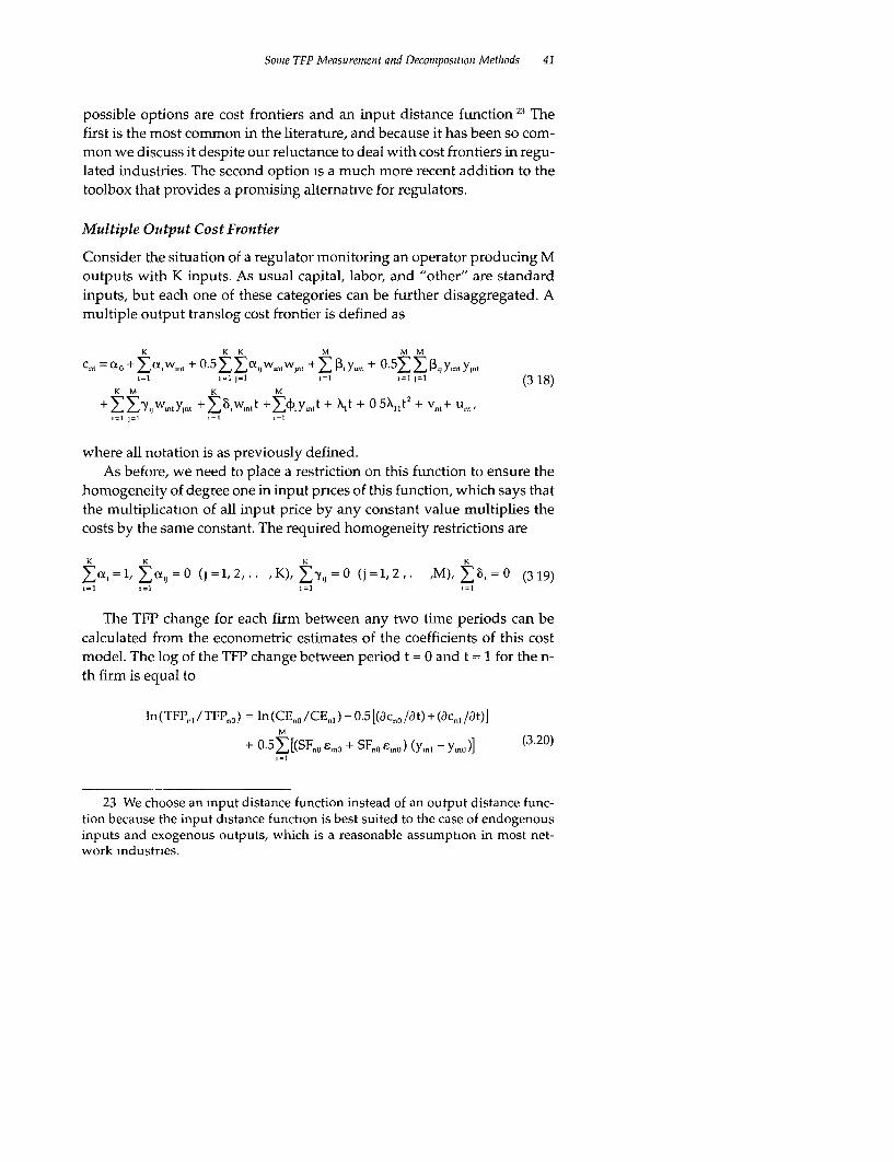
Sonme TFP Measurement and Decompositioni Methods 41

possible options are cost frontiers and an input distance function 23 Thefirst is the most common in the literature, and because it has been so com-mon we discuss it despite our reluctance to deal with cost frontiers in regu-lated industries. The second option is a much more recent addition to thetoolbox that provides a promising alternative for regulators.

Multiple Output Cost Frontier

Consider the situation of a regulator monitoring an operator producing Moutputs with K inputs. As usual capital, labor, and "other" are standardinputs, but each one of these categories can be further disaggregated. Amultiple output translog cost frontier is defined as

K K K M M M

Cnt =ao +Zcwmt+w + 05Y +3y m , + 05 Pq Ymt Y1ml=l =1 I=l z=l I=l §=l ~~~~~~~~(3 18)

K M K M

+ 'Ylw,nWy,n, +BXnl,,t +E¢4)y,n,t + Att + 0 5X1 1t2

+ Vnt + Unt,

where all notation is as previously defined.As before, we need to place a restriction on this function to ensure the

homogeneity of degree one in input prices of this function, which says thatthe multiplication of all input price by any constant value multiplies thecosts by the same constant. The required homogeneity restrictions are

K K K K

o, = 1, Eoa, = 0 (j = 1, 2.. , K), -y,l = 0 (j = 1, 2. ,M), 8, = 0 (3 19)1=1 *=.=*1

The TFP change for each firm between any two time periods can becalculated from the econometric estimates of the coefficients of this costmodel. The log of the TFP change between period t = 0 and t = 1 for the n-th firm is equal to

In (TFP,, /TFP,, 0 ) = ln (CEn, /CEnl ) -0.5 [(acn0 /at) + (aCnl /at)]M

+ 0.5Z [(SF,, e,, + SF,, e,,O) (yml - Yrno)] (3.20)-1=

23 We choose an mput distance function instead of an output distance func-tion because the input distance function is best suited to the case of endogenousinputs and exogenous outputs, which is a reasonable assumption in most net-work industries.

42 A Primer on Efficiency Measuremenitfor Utilities and Transport Regulators

where the three terms on the right-hand-side of equation (3.20) are the CEC,TC, and SEC terms, respectively. 24 'he cost efficiency measure, CEn,, is thesame as specified for the single output case. The technical change measu,eis the mean of the technical change measures evaluated at the period 0 andperiod 1 data points. For firm n in period t this is

K M1

ac,, /at = X1 + kl+t + B + E( X ld *) (3.21)

The final term in equation (3.20), which -neasures the change in scaleefficiency, requires calculation of the output elasticities

M= acn./yY,M= I= +YP,,,y, 1 + -y,w,t+<h (322)I * I

for each output at each data point, and the calculation of the scale factorsK

SFnt = (e 1n- 1)/-nt at each data point, where -41t I`

Once more, just as in the single output. cost frontier case, with infornma-

tion on input quantities and output prices a Timovist TFPC index (see eqtla-tion 3.6) can be calculated as

MIn(TFPn,/TFPn0 ) = 0.5 E [(r_nl ' r1,,).(y1 n- y-.0)]

K ~~~~~~~~~~(3.23)0.5 E [(s.,+ s,0 )-(x., - x.,),

where rjnl is the revenue share of the j-th output for the n-th firm in the t-thyear. The difference between equation (3.23) ancd the cost-based TFrp ind ex

(equation 3.20) is equal to the allocative inefficiency measure as follows:

24 This decomposition is based on that presented in I(umbhakar and Lox cll(2000), which was derived using total differential methods. However, we have con-verted their differential formula into an index number formula, as we did in .he

smgle output cost frontier.25. This is equal to the inverse of the standard returns to scale elasticity. iN\cx

that if we have constant returns to scale, this will equal 1, and hence the scale ;e,min equation (3.20) will be equal to 0, as required.

Some TFP Measurement and Decomposition Methtods 43

K

AEC = 0.5 E ([ (Ki,1 - Sm,) + (Kl - S_0 )] J(W,i, W-O) )

+ 0 5 ([(mnl - r,. 1) + (7rrnO - r,.O)]-(y, 1 - Y'O). (3.24)

The interpretation of this measure is somewhat more complex, as it con-tains two parts. The first part is due to input mix allocative inefficiency.That is, when the observed cost shares, smt, differ from the efficient costshares

K M

Kk,l,= Cnl /aWk, = ak+ ykxWrt + ljY,t + kt (3 25)

The second part of equation (3.24) is due to output mix allocative ineffi-ciency. That is, when the observed revenue shares, r,,t, differ from the effi-

cient revenue shares lTmnt = 8.t/-nt' that is, when shadow prices deviatefrom market (observed) prices.2 6

Input Distance Function

Increasingly, regulators are likely to come across input distance functionsin the literature on efficiency measures in their sector (see Coelli andPerelman 1999,2000 for applications to the railways sector and Carrington,Coelli, and Groom 2002 for an application to gas distribution). An inputdistance function can be thought of as a multiple output version of a pro-duction frontier. It considers the amount by which the input set of eachfirm may be proportionally contracted with the output set held fixed. Thisliterature is somewhat more technical, but it is worth going through in somedetail, as it is likely to become an important new instrument for analyzingefficiency in multi-output sectors. 27

26. Most regulated firms face fixed input prices and fixed output quantities.Thus improvements in input mix allocative efficiency can be sought via adjust-ments to input quantities, while improvements in output mux allocative efficiencyare sought through adjustments to the output prices, that is, tariff rebalancing

27. Note that nonparametric input distance functions (input-oriented DEA mod-els) have already been used in a number of regulatory analyses.

44 A Pnmer on Efficiency Measurement for Utilities and Transport Regulators

A translog input distance function witlh M outputs and K inputs maynow be specified as

d, = ot, + E Ynt + 2 Y., Y., + Klx' kN + I K ntm I m 1~ I ic 1 k 1 I

K M K VI (3.26)+ZZYkmX IntY_t+Z ;bXltt+X(Z,yL,ti -1- X,i + 0.5X1IJ2

k-lm I 1 i I

where d., is the log of the input distance, Ynt and x,.t are as defined before,and the Greek letters represent parameters to be estimated.

A necessary property of the input distance function is homogeneity (ofdegree +1) in inputs, which implies that

K K K l;

ZUk =1, Zcxk=0 (k = 1, 2, ., K), E = (k =1,2.. ), = O . (3.27)k-I I I l I I

Imposing these restrictions upon equation (3.26) yields the estimatingform of the input distance function, in which the distance term, dnm, can beviewed as an error term as follows,

M M \lN 1

XK =Cx +OEt mYmnt + 2 y X , In Ymt + a I,(xt,.t xCnt)m I m 1,l1 1. 1

K I K I K I \i

+ - (xk-(X 1 - xi't)(xpt - x1 R,1 )+ 7y, 1(x 1Q 1- XKJ,)Ym-tk-I I 1 I n I

K-1 M

+Z;8(x.t,- x1m,)t +7¢t,y.,t + X,t+0.5X,t2 - d, (3.28)

This error term explains the difference between the observed data pointsand those points predicted by the estimated transformation function. ))V'can replace the distance term, -d,1 , with a composed error term, v.,- u-,and estimate this function as we would do for a standard stochastic fron-tier function.

Now to measure TFPC relative to this estimated function we calculate 25

28. Here we follow the general approach outlined in Orea (2002); however, wehave adjusted the output distance function mefhod in Orea (2002) to suit the inputdistance function used here

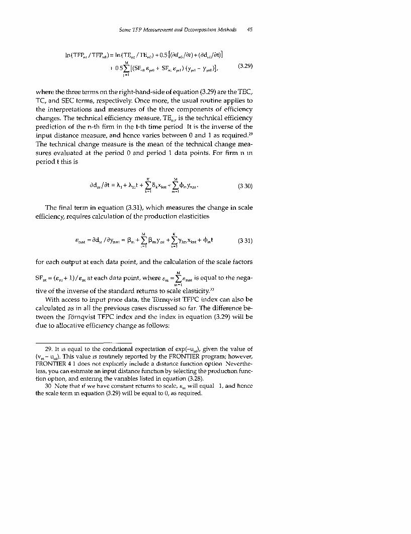
Some TFP Measuremnent and Decomposition Methods 45

ln(TFPn1 / TFPn) = In(TEn, /TE.,) + 0.5 [(adnl/at) + (adl,/at)]

+ 0 5 [(SFno ep. + SFn, niJ) (Ynl - Yjn0)]1 (3.29)1=i

where the three terms on the right-hand-side of equation (3.29) are the TEC,TC, and SEC terms, respectively. Once more, the usual routine applies tothe interpretations and measures of the three components of efficiencychanges. The technical efficiency measure, TEn1, is the technical efficiencyprediction of the n-th firm in the t-th time period It is the inverse of theinput distance measure, and hence varies between 0 and 1 as required.2 9

The technical change measure is the mean of the technical change mea-sures evaluated at the period 0 and period 1 data points. For firm n inperiod t this is

K M

addn lat = X, + XAlt + °kXk,,t + Ymnt (3 30)k=1 -I=

The final term in equation (3.31), which measures the change in scaleefficiency, requires calculation of the production elasticities

M K

8mnt = add, /aymn, = 3m + E Pr.Ymnt + lYkmX., + 4kmt (3 31)-1= k=1

for each output at each data point, and the calculation of the scale factors

M

SFn1 = (en, + 1) / 8 n, at each data point, where en, = E e_, is equal to the nega-m=l

tive of the inverse of the standard returns to scale elasticity. 0

With access to input price data, the Tornqvist TFPC index can also becalculated as in all the previous cases discussed so far. The difference be-tween the Tbrnqvist TFPC index and the index in equation (3.29) will bedue to allocative efficiency change as follows:

29. It is equal to the conditional expectation of exp(-un1 ), given the value of(vn - unl). This value is routmely reported by the FRONTIER program; however,FRONTIER 4 1 does not explicitly include a distance function option Neverthe-less, you can estimate an input distance function by selecting the production func-tion option, and entering the variables listed in equation (3.28).

30 Note that if we have constant returns to scale, es, will equal -1, and hencethe scale term in equation (3.29) will be equal to 0, as required.

46 A Primer on Efficzency Measurenient fiur Utilites and Transport Regulators

AEC= 0-5 {[ (rm, + sme/,ni ) + (r_ 0 + _mn0 /E,O)] (Ymnl -y_,)l

K ~~~~~~~~~~~~~~~(3.32)° 5 E ([(skl- e.) + (s,,,,- e,., 1)] (x,n- x,,.(.)))

k 1

Equation (3.32) has two components. The first measures output mixallocative efficiency effects. It will be nonzero if the market output shares,r,,,,, differ from the shadow output shares, 8mni/£ni, and if the output mix

changes. Note that the shadow output shares will equal the out-put elastLici-ties, Smnt, only under constant returns to scale, that is, when e,, = -1. 'ihesecond component in equation (3.32) measures input mix allocative effi-ciency effects. It will be nonzero if the market input shares, sk,t, differ fromthe shadow input shares

M

e., = 8d,,1 /lxk.t = Clk + Ec,,x, + XYi. Ymnt + 8kt, (333)

and if the input mix changes.Some authors, such as Rodriguez-Alvarez 2000, argue that the econo-

metric estimation of distance functions can be improved by the addition ofcost share equations. For example, if you believed that cost minimizationwas a reasonable assumption (a questionable assumption in most networkindustries) and you had data on input cost shares, you could estimate theinput distance function along wi'h K - I input share equations, defined byequation (3.33), in a system of equations. However, no "canned" compu'.erpackage allows thls option, and you therefore have to do che programmingfrom scratch. Alternatively, you could use the standard seemingly unre-lated regressions method to estimate this system, which assumes all errorterms are symmetric, and then adjust the intercept in the distance functionusing some type of corrected OLS method.3"

31. Furthermore, you could test the cost-minimi7ing assumption by testing thehypothesis that the ot,s in the share equations equal the (x,1s in the distance func-tion If this was rejected you could replace the u,,s in the share equations withdifferent parameters, say 9,s. This would convert the system to a shadow cost-miimizing system, where nonzero values of (c,, - . ) would reflect a differencebetween the shadow price and the market price for the k-th input This is as donein Alvarez (2000) This appears to be a much cleaner way to deal with this issuethan the shadow cost function approach suggested by Balk (1998) and others.

Sonie TFP Measurement and Decomposition Methods 47

In many respects one could argue that the input distance function shouldbe the function of choice in analyses of TFP in network industries. First, itavoids the problems associated with the cost function approach when costminimization is violated. Second, it is much less complicated than theshadow cost function approach Moreover, it permits having multiple out-puts in a primal setting and avoids the endogenous regressors criticismthat is sometimes leveled at the production frontier approach (see Coelli2000 for more on this endogeneity issue).

However, having listed the advantages of the distance function approach,we hesitate to provide a strong recommendation for its use by the averageregulator, given that it is such a new methodology. Perhaps it may be bestfor most regulators to wait a year or two before embracing distance func-tions. This will allow time for those regulators with access to high-leveleconometric expertise to put the method through its paces. Once this hasbeen completed, we expect that input distance functions will become themethod of choice in regulatory analyses.

In the meantime, you can avoid estimating a distance function by usingPIN to aggregate outputs and then estimating an SFA production frontier.Alternatively, you could use PIN to aggregate inputs and then estimate anSFA input requirements frontier, that is, you regress an index of inputsagainst a vector of outputs. This latter strategy has the virtue of being consis-tent with the resource-conserving orientation of most utilities.

Malmquist DEA TFP Indexes

In this section we describe how a Malmquist TFP index can be con-structed using input distance functions and how to estimate these inputdistance functions using DEA-like methods. Our methods are based onthose outlined in Fare and others (1994), who used output distance func-tions. The input- and output-oriented approaches give identical TFPmeasures, but can provide slightly different scale efficiency decomposi-tions. The input distance function is the natural one to use in regulatedindustries, where endogenous input quantities and exogenous outputquantities are the norm.

The Malmquist TFP index measures the TFP change between two datapoints by calculating the ratio of the distances of each data point relative toa common technology. The Malmquist (input-oriented) TFP change indexbetween period 0 (the base period) and period 1 (using period 1 technol-ogy as the reference technology) is given by

48 A Prmner on Efficiency Measurenient for Utilities and Transport Regulators

TFPJ/TFPO = D'(Y",X0 ) (3.34)D1 (Y1,IX I)

where the notation D,(Y0 X0) represents the distance from ,he period 0 ob-servation to the period 1 technology. A value of the ratio in equation (3.34)greater than 1 will indicate a TFP improvement, for example, a value of1.04 corresponds to a 4 percent increase in TFP. 32

An alternative Malmquist index can also be defined relative to the pe-riod 0 technology. Indeed, Fare and others (1994) defined their Malmqu-istTFP index as the geometric mean of these two indexes, that is, one evalu-ated with respect to period 1 technology and the second with respect toperiod 0 technology. Doing this yields

[ D, (Y.~, X) D, (Y," ,x ) 0 TFP, / TFPo = D1 (Y°,X) DM(Y° X°)] (3.35)

An equivalent way of writing this productivity index is

TFPI/TFPO D-(Y DX.) FD(Y 0,X0 )D1 (Y3,D1(Y1,X1) [D 0 (Y0,X.) D(YiX)j' (3.36)

where the ratio outside the square brackets measures the change in theinput-oriented measure of technical efficiency between periods 0 and I (re-call that the input distance measure is the inverse of the input-orientedtechnical efficiency measure).3 3 The remaining part of the index in equation(3.36) is a measure of technical change. It is the geometric mean of the shif.in technology between the two periods, evaluated at the period 0 data pointand also at the period 1 data point.

32. Note that in this section we present our TFP indexes in ratio form instead ofthe log-change form used in the previous sections. This is because the translogfunctional form naturally lends itself to the calculation of T-FP change in log-changeform. When we make our empirical comparison in chapter 4 we will take the loga-rithms of our DEA results to make them comparable with our translog and Tbrnqvistresults.

33. Farrell measures of efficiency correspond in each case to the expression orthe reduction of the ray that passes through the origin (see Farrell 1957).

Some TFP Measurement and Decomposition Methods 49

For most regulators of infrastructure services, however, the foregoingTFP index may not be a good option. Indeed, for the index in equation(3.36) to measure TFP change properly, CRS distance functions are required,otherwise the implicit weights will not add up to 1, and thus any scaleefficiency gains (or losses) will be missed. Fare and others (1994) used CRSdistance functions to calculate the index in equation (3.36). They also sug-gested a further decomposition of equation (3.36) whereby the CRS techni-cal efficiency change measure could be decomposed into a "pure" technicalefficiency change component and a scale efficiency change component. Thisis done by introducing some VRS distance functions to obtain

TFP1/TFPO D= (Y,X 0 )-I [(Y, XI) DC(YO XO)]' ° DV~(Y,,X,)[Dv (Y,,,X,,) Dc(Y,,X,)]

x Dc(YO XO)Dc(Y1,XJ1) (3.37)LDC(YO ,XO) DOc(Y,,X,)J

where the V and C superscripts refer to VRS and CRS technologies, respec-tively Equation (3 37) thus gives a TEC measure, an SEC measure, and aTC measure, that is

TFPC = TEC x SEC x TC. (3.38)

Some authors have criticized this decomposition because it measurestechnical change against the CRS technology instead of the VRS technol-ogy Various alternatives have been proposed; however, none has yet gainedwidespread acceptance (see Balk 1999 and Grifell and Lovell 1999 for adiscussion of this issue).

Fare and others (1994) showed that, given the availability of suitablepanel data, we can calculate the required distances in equation (3.37) usingDEA-like linear programs. These calculations are implemented in the com-puter program: data envelopment analysis program (DEAP) 2.1.3 See chap-ter 7 m CRB for further details on the DEA programs involved.

Fmally, note that Malmquist DEA TFP indexes use shadow prices, justlike their parametric counterparts (translog production and distance func-tions) discussed earlier, and hence do not account for allocative efficiency

34. See Coelli (1996a) for more on the DEAP computer software. This softwarecan be downloaded from http-//www uq edu au/econonucs/staff/coelli htm

50 A Prnter on Efficiency Measurement for Uttities and Trannsport Regulators

changes. Calculating the Tornqvist index and interpreting any differenlcosbetween the two measures as being primarily due to allocative efficiencyeffects is fine, but note that this allocative efficiency change measure willbe a combination of input mix and output m-Lix allocative efficiency. An ad-vantage of the parametric decomposition methods is that you can obtainseparate measures of these two components."

Cross-Sectiona1l TFIFI C¢Domnpins

All the discussion in this chapter thus far has concenirated on the case wherewe wish to measure (and decompose) the TFPC for a firm between twotime periods. Sometimes, however, the regulator needs to compare the TFPof a group of firms at one point in time. This is at the core of comparativeperformance evaluation for any regulator and is the key to effective yard-stick competition. Consider a case where the regulator is monitoring Noperators of quasi-competitive firms, typically local monopolies. This couldbe a group of regional ports or provincial water or electricity distributioncompanies. With N operators the regulator can construct N(N - 1) pair-wise comparisons. The problem in that case is that standard Laspeyres,Paasche, Tornqvist, and Fisher indexes are nontransitive, that is, the pair-wise comparisons will not necessarily give the same ranling of operators.For example, consider firms A, B, and C. We may calculate TFP indexes ofI(AB) = 1.1 and I(BC) = 1.1 and I(AC) = 1.15, that is, A is 10 percent betterthan B, B is 10 percent better than C, and A is 15 percent better than C.These three indexes are not consistent, because we should have found thatA was 21 percent better than C (1.1 x 1.1 = 1.21).

Thus we need to "adjust" these inconsistent indexes to produce conss-tent indexes. The method most often used is thne so-called EICS methcl,based on Elteto and ICoves (1964) and Szulc (1964) (see chapter 4 in CR3).Caves, Christensen, and Diewert (1982a) showed that in the case of theTomqvist index, there is a way to produce an adjusLed T6mqvist index wh Xre

35. Creativity can help minimize the damage somewhat. TU, for example, youhave input prices but not output prices, say in a study of public hospitals, youcould use the shadow revenue shares from the DEA (see Coelli and Rao 1999 forhow to calculate these), along with the actual cost shares in the calculation of aTlrrqvist index. The difference between this TFPC index and the Malmquist D 3ATFP index should reveal information about the contribution of input-mix allocativeefficiency.

Some TFP Measurement and Decomposition Methods 51

a pair of firms is compared indirectly via the sample mean firm based onthe EKS method. That is, by adjusting equation (3.4) we obtain

M M

In(TFP.l /TFP )T(EKS) =0 5 [(r1 + r).(y. - Y )]- 0.5 _[(r,.O+ F,) (Y-nO Y)]1=1 (3.39)

K ~~~~~~~K-O 5 RS, [s + 9, ) (x.,,\- x, ) ] + ° 5RE[Sm.o + 9- ) (X, mO x, )]

,=1,=

where-r, is the j-th output share at the sample mean and s, is the i-th inputshare at the sample mean. Note that when one observation is added orsubtracted from the sample, we must recalculate all indexes in this case,because the sample means will change.

The decomposition of the TFP difference between two firms at one pointin time (into TE, SE, and AE components) can be done in an identical wayto that described for the time comparison, except that TC will not be anissue. However, in some cases the regulator may specify that it is only in-terested in TE comparisons across firms (it may perhaps believe that scaleand AE are not controllable in the short run). In this case we need not botherwith the between firm decomposition calculations, because the technicalefficiency measures themselves will be sufficient.

What if Policy or Other Similar Variables Are Relevant?

Our examples so far do not include any environmental variables in themodel, and yet these may be quite relevant. Changes in regulatory regimes,shocks such as the 1997 Asian financial crisis, weather patterns, or similarvariables are often important here The good news is that extending themethod to include a term for environmental differences, either across firmsor time, is easy. Indeed, we could view the time trend (technical changeproxy) as a Z variable. If we do this we can see quite clearly how to calcu-late the effect of environment change, which we can label ZC Instead ofhaving partial derivatives with respect to time, we will have partial deriva-tives with respect to the Z variable(s), and so on.

Where do we include the Z variables? Do we put them in the translogfunction like a regular regressor variable or as part of the inefficiency errorterm in the SFA model as done in Battese and Coelli (1995)? The discussionof this option is beyond the scope of this book, but chapter 9 in CRB; Batteseand Coelli (1995); and Coelli, Perelman, and Romano (1999) provide somediscussion. The latter paper stresses that one must be careful when

52 A Primer on Efficiency Measuremeat for Utilities and Troaisport Regilators

interpreting efficiency scores in the different models. The main point .oremember is that if the Z variable is included in the translog function, theefficiency score obtained will be net of the efrfeci of .he Z variable, while ifthe Battese and Coelli (1995) model is used, one obtains gross efficiencyscores, where the effect of the Z variable is included in the efficiency score.

Surmming Up

Table 2.3 summarized the three main methods of performance measur,-ment, including the main advantages and drawbacks of each approacn,

and emphasized the types of concems a regulator should have. On the dat.aside, for instance, assessing up-front the restrictions imposed on the meth-odology choice by the data is crucial. SFA and DEA are quite demanding inthis respect. After a few years of operation, a regulator should have beenable to generate enough information to be able to begin to use these me,'h-ods in a detailed way. At the outset of their operations, however, most regu-lators will have to pick between using PIN or a restricted form of SrA orDEA, for example, impose constant returns to scale, use a simple functionalform, aggregate inputs and outputs into only a E-ew measures.

A look at the relative advantages of each method in table 2 3 shows thatone advantage of SFA is that it is more amenable to modeling the effects ofenvironmental variables than DEA. In the longer run, SFA methods aredifficult to ignore, as demonstrated by the United Kingdom's experience,where they lie at the core of the policy debates between producers and

regulators. The potential offered by these methods has to be balanced bytheir drawbacks, which in practice can be significant because they requirenot only good judgment, but also good econometric skills.

If the regulator chooses the SFA method, it must then choose betweenthe cost frontier and production frontier approaches. These two functiohmscan (and often do) provide differing results. The biggest differences ivilloccur when there are large allocative distortions. This can be particula, lyimportant in regulated industries, where various factors such as the Averchand Johnson (1962) effect can introduce significant allocative distortions.When there are such allocative distortions, the estimates of the parametersof the cost frontier will be biased, and hence the various efficiency decom-n-positions will also be biased.36 Moreover, even if all firms are allocatively

36 This issue regarding the estimaion of cost frontiers in the face of systematicallocative distortions is rather complex. Our concern primarily relates to the casewhen we wish to use the cost frontier estimates to decompose efficiency change

Some TFP Measurement and Decomposition Methods 53

efficient, the directly estimated production frontier need not be identical tothe production frontier implied by the estimated cost frontier. This is sim-ply because a different object function is being maximized. Finally, notethat allocative mefficiency need not only be the result of regulatory distor-tions, but can be due to various other factors, such as measurement errors,optimal long-run plans appearing to be suboptimal in the short run (typi-cal in infrastructure industries), poor management decisions, or unexpectedprice changes or demand changes. The upshot of all this is that carefulinterpretation of results is always required. Furthermore, given the pos-sible bias in cost frontier estimates in the presence of allocative inefficiency,one could argue that the production frontier approach is the preferredmethod for use in regulated industries. We discuss method choice in moredetail later.

Finally, of the measurement methods discussed in this chapter, SFA andDEA have the advantage in that they allow a detailed decomposition ofperformance. The contribution of each factor to TFP-change in technol-ogy, technical efficiency, allocative efficiency, and scale efficiency-eitherat the firm level or the industry level, can be identified. They offer the regu-lator access to detailed information, which can help improve the quality ofregulatory decisions.

mto technical and allocative components. If we do not need to do this, then costfrontier estimation should be alright. That is, one can still estimate a cost frontierand measure the amount by which the firms become closer to or further away fromthe frontier to obtam cost efficiency change measures and measure the amount bywhich the cost frontier shifts over time to obtain a technical change measure (whichshould be a reasonable indicator of the shift m the production frontier if there hasnot been any systematic change in allocative efficiency durmg the sample period).

4

An Empirical Example

Consider a regulator that must monitor the performance of 20 railway com-panies. The regulator has annual data on the 20 railways over a five-yearperiod. The data for this exercise have been randomly generated, but theyprovide the same kind of diversity that would be observed in the real world.Each firm uses three inputs, capital, labor, and other, to produce one out-put, measured in passenger kilometers.

The data, which are listed in table 4 1, have been generated as follows:

* Cobb-Douglas technology was used for data generation (a translogis used for estimation)

* Elasticities of capital, labor, and other are 0.40,0.30, and 0.30, respec-tively, and hence the return to scale elasticity is 1.0

* Neutral technical change is 2 percent per year* Technical efficiency change of approximately 1 percent occurs be-

tween years 2 and 3* No scale efficiency change occurs* No allocative efficiency change occurs* No systematic (mdustrywide) allocative inefficiency is present, but

a small amount of random allocative errors take place at the firmlevel.

We have used this data to measure TFP changes for each firm using

* Tornqvist PIN* SFA production function* SFA cost function* SFA input distance function* Malmquist DEA.

55

56 A Primer on Efficiency Measurementfor Utieities end Tranisport Regulaltors

Table 4.1. Ratlzways Data

Quantities Prices

Firm Year Output Capital Labor Othler Capital Labor Ollier

1 1 25.665 21.440 10.143 9.083 6.411 8.958 10.8972 1 29.024 22.254 11.504 10.402 7.805 10.151 11.6583 1 25.600 16.151 12.525 9 829 7.846 8.842 10.2734 1 23.046 17.763 11.597 10 336 7.341 9.136 10.952

5 1 30 573 23.679 11.800 12.642 7 152 10.711 10.411

6 1 25.557 17.497 12.811 10 091 7.851 10.024 11.2107 1 28.988 21.214 9.985 8.962 6 752 10.295 12.1'708 1 24.233 17.347 9.116 8.203 8.435 9.409 11 6609 1 23.498 17.534 10.019 9.452 7.721 9 871 10 916

10 1 28.226 22.079 11.167 11.300 7 739 10.063 11.83811 1 23.121 22.861 12.415 7.831 6.468 9.076 11.41512 1 29.635 23 500 12.150 9.556 6 159 8.768 12.2 1613 1 21 035 16.985 9.410 8.332 7 389 10.262 11 56814 1 24 970 21.157 9.346 8.156 7168 10 103 10 83715 1 31.553 23.097 11.203 10.116 6.474 10.529 10.32116 1 21.575 15.638 11.081 7.097 7.043 9.455 11.91217 1 28.402 20.891 9 600 10.859 7.433 10 536 11.56218 1 26.275 18.613 11 290 9.130 7.890 9.915 12.32819 1 23.435 18.603 8.496 7.346 7.172 10 019 12.41520 1 30.709 22 958 12.028 10.574 6.908 9.389 12.026

1 2 27933 18.928 12.666 8.877 6.573 8.590 10.269

2 2 29.423 21 593 11.818 11.417 7.927 10.912 11.7453 2 28.040 20.033 11.861 9.465 7.715 9.194 10.9864 2 28.583 20.156 10.547 8.510 7.374 9.965 11.4137

etc.

16 5 23.141 14.194 9.673 8.108 7022 9.545 11.60917 5 31.264 16 767 11.515 10.514 7.549 10.374 10.78918 5 24.785 16.614 12 143 9.875 8.039 9.917 12.06319 5 25.980 21.780 8 589 8.046 7.293 10.892 12.66620 5 30.742 24.233 10.510 8.829 6.389 10.267 11.977

All details on the estimation and calculation of our results are listed in azip file, eg.zip, that can be found on the web site www.worldbank.o:-g/wbi/regulation/efficiencybook. We calculated the results using both Exceland Shazam. In this chapter we will explain in some detail how the SPAproduction function results were obtained and then compare the resultsobtained using all five methods.

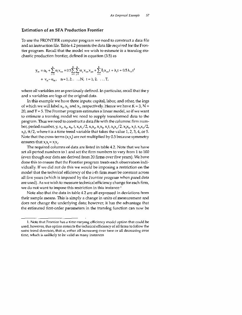
An Empirical Example 57

Estimation of an SFA Production Frontier

To use the FRONTIER computer program we need to construct a data fileand an instruction file. Table 4.2 presents the data file required for the Fron-tier program. Recall that the model we wish to estimate is a translog sto-chastic production frontier, defined in equation (3.5) as

K K K K

Yt= (o + YCiX. +0 .5YY"jXlntX +Y8,Xmtt + X1t + 0.5XA,t'-I = =1 j=1

+ vnt-unt, n=1,2,. .,N, t=1,2, .T,

where all variables are as previously defined. In particular, recall that the yand x variables are logs of the original data.

In this example we have three inputs: capital, labor, and other, the logsof which we will label x,, x2 and x3, respectively. Hence we have K = 3, N =20, and T = 5. The Frontier program estimates a linear model, so if we wantto estimate a translog model we need to supply transformed data to theprogram. Thus we need to construct a data file with the columns: firm num-ber, period number, y, xl, X2. X3, t, x 1xj/2, x1x2, xlxX, xlt, x2 x2 /2, x2x3, x2t, x3 x3 /2,x3t, tt/2, where t is a time trend variable that takes the value 1, 2, 3, 4, or 5.Note that the cross-terms (x,x,) are not multiplied by 0.5 because symmetryensures that x,x = x1x,.

The required columns of data are listed in table 4.2. Note that we haveset all period numbers to 1 and set the firm numbers to vary from 1 to 100(even though our data are derived from 20 firms over five years). We havedone this to ensure that the Frontier program treats each observation indi-vidually If we did not do this we would be imposing a restriction on themodel that the technical efficiency of the i-th firm must be constant acrossall five years (which is imposed by the Frontier program when panel dataare used). As we wish to measure technical efficiency change for each firm,we do not want to impose this restriction in this instance l

Note also that the data in table 4.2 are all expressed in deviations fromtheir sample means. This is simply a change in units of measurement anddoes not change the underlying data; however, it has the advantage thatthe estimated first-order parameters in the translog function can now be

1. Note that Frontier has a time-varying efficiency model option that could beused, however, this option restricts the technical efficiency of all firms to follow thesame trend direction, that is, either all increasing over time or all decreasing overtime, which is unlikely to be valid m many instances

Table 4.2. Contents of Frontier Data File (pfn.dta)

Firm Year y xl x2 x3 t xlxl/2 xlx2 xlx3 xlt x2x2/2 x2x3 x2t x3x3/2 x3t tt/2

1 1 -0 05445 0.09343 -0 07618 -0.02310 -2 0 00436 -0 00712 -0 00216 -0 18686 0 00290 0.00176 0 15236 0 00027 0 04621 22 1 0.06857 0.13070 0.04969 0 11245 -2 0 00854 0 00649 0 01470 -0 26140 0 00123 0 00559 -0.09938 0 00632 -0 22490 23 1 -0 05695 -0 18988 0 13469 0 05575 -2 0 01803 -0.02557 -0.01059 0 37976 0 00907 0.00751 -0 26937 0 00155 -0.11149 24 1 -0 16208 -0 09473 0 05777 0 10612 -2 0.00449 -0.00547 -0 01005 0 18946 0 00167 0 00613 -0 11554 0.00563 -0.21223 25 1 0 12056 0.19277 0 07510 0 30744 -2 0.01858 0 01448 0 05927 -0 38554 0 00282 0 02309 -0.15020 0 04726 -0 61489 26 1 -0 05863 -0.10980 0.15730 0 08210 -2 0 00603 -0 01727 -0 00901 0 21961 001237 0 01291 -0.31460 0 00337 -0 16419 27 1 0 06731 0 08281 -0.09193 -0 03656 -2 0.00343 4 00761 -0 00303 -016562 0 00423 0.00336 0.18386 0.00067 0 07313 28 1 -0 11185 -0 11839 -0 18298 -0 12502 -2 0.00701 0 02166 0.01480 0 23678 0 01674 0.02288 0 36595 0 00781 0 25003 29 1 -0.14264 -0 10771 -0 08852 0 01666 -2 0 00580 0 00953 -0 00179 0.21542 0.00392 -0 00148 0 17703 0.00014 -0.03333 2

10 1 0.04067 0 12277 0.01994 0 19521 -2 0 00754 0 00245 0 02397 -0 24555 0 00020 0.00389 -0 03987 0 01905 -0 39042 211 1 -0 15881 0 15760 0 12592 -0 17149 -2 0.01242 0.01985 -0 02703 -0 31520 0 00793 -0.02160 -0.25185 0 01471 0 34299 212 1 0.08941 0.18515 0 10435 0 02760 -2 0.01714 0 01932 0.00511 -0.37031 0 00544 0 00288 -0.20870 0 OC038 -0.05520 213 1 -025337 -0.13949 -0 15124 -0 10947 -2 0.00973 002110 001527 027899 0.01144 001656 030248 000599 0.21894 214 1 -0 08190 0.08015 -0.15801 -0 13079 -2 0 00321 - 01267 -0 01048 -0 16031 0 01248 0 02067 0 31602 0 00855 0 26159 215 1 015211 0.16786 002314 0.08459 -2 001409 000388 0.01420 -0.33573 000027 000196 -004627 0.00358 -016917 216 1 -022801 -0.22214 0.01224 -026985 -2 002467 -0.00272 005994 044429 0.00007 -0.00330 -0024418 003641 0 53969 217 1 0 04691 0.06749 -0 13124 0.15548 -2 0 00228 -0 00886 0 01049 -0 13498 0 00861 -0 02040 0 26248 0 01209 -0 31095 218 1 -0 03094 -0.04797 0.03090 -0.01800 -2 0 00115 -0 00148 0.00086 0 09594 0 C0048 -0 00056 -0.06180 0.00016 0 03601 219 1 -0.14533 -0.04851 -0.25343 -0 23546 -2 0.00118 0 01229 0 01142 0 09701 0.03211 0 05967 0 50686 0.02772 0.47093 220 1 0 12499 0 16183 0.09426 0 12883 -2 0 01310 0 01525 0 02085 -0 32367 0.00444 0.01214 -0 18851 0 00830 -0 25766 221 1 0 03024 -0 03121 0 14589 -0.04613 -1 0 00049 -0.00455 0 00144 0 03121 0 01064 -0.00673 -0.14589 0 001C6 0 04613 0 522 1 0 08220 0 10053 0 07658 0.20553 -1 0 00505 0 00770 0.02C66 -010053 0 00293 0 01574 -0.07658 0.02112 -0 20553 0 5

etc

98 1 -0 08932 -0.16157 0 10373 0.06048 2 0 01305 -0 01676 -0 00977 -0 32315 0.00538 0 00627 0 20746 0 00183 0 12096 299 1 -0 04225 0.10915 -0.24247 -0.14437 2 0 00596 -0.02647 -0.01576 0 21830 0.02940 0 03501 -0 48495 0.01042 -0.28875 2

100 1 0 12607 0 21586 -0 04068 -0.05154 2 0 02330 -0.00878 -0.01113 0 43172 0 00083 0 00210 -0 08136 O.C0133 -0.10308 2

Note Column head:ngs do not appear in the data file, only data Also note thai Lhe data m tliis table are prcesnted to five decimal places In ihc act'l, I OM

file, all available decimal places appear

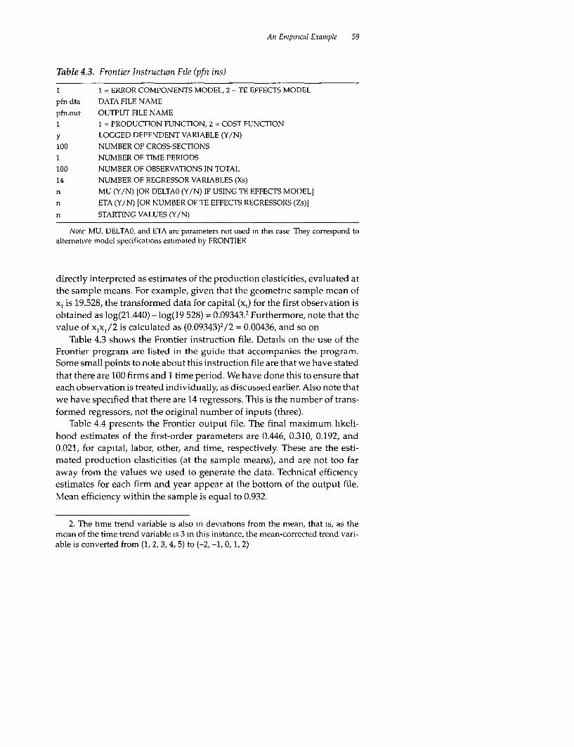
An Empirical Example 59

Table 4.3. Frontier Instruction File (pfn ins)

1 1 = ERROR COMPONENTS MODEL, 2 = TE EFFECTS MODEL

pfn dta DATA FILE NAME

pfn.out OUTPUT FILE NAME

1 1 = PRODUCTION FUNCTION, 2 = COST FUNCTION

y LOGGED DEPENDENT VARIABLE (Y/N)

100 NUMBER OF CROSS-SECTIONS

1 NUMBER OF TIME PERIODS

100 NUMBER OF OBSERVATIONS IN TOTAL

14 NUMBER OF REGRESSOR VARIABLES (Xs)

n MU (Y/N) [OR DELTA0 (Y/N) IF USING TE EFFECTS MODEL]

n ETA (Y/N) [OR NUMBER OF TE EFFECTS REGRESSORS (Zs)]

n STARTING VALUES (Y/N)

Note MU, DELTA0, and ETA are parameters not used in this case They correspond toalternative model specifications estimated by FRONTIER

directly interpreted as estimates of the production elasticities, evaluated atthe sample means. For example, given that the geometric sample mean ofxi is 19.528, the transformed data for capital (xl) for the first observation isobtained as log(2 1.4 4 0 ) - log(19 528) = 0.09343.2 Furthermore, note that thevalue of x1 x,/2 is calculated as (0.09343)2/2 = 0.00436, and so on

Table 4.3 shows the Frontier instruction file. Details on the use of theFrontier program are listed in the guide that accompanies the program.Some small points to note about this instruction file are that we have statedthat there are 100 firms and 1 time period. We have done this to ensure thateach observation is treated individually, as discussed earlier. Also note thatwe have specified that there are 14 regressors. This is the number of trans-formed regressors, not the original number of inputs (three).

Table 4.4 presents the Frontier output file. The final maximum likeli-hood estimates of the first-order parameters are 0.446, 0.310, 0.192, and0.021, for capital, labor, other, and time, respectively. These are the esti-mated production elasticities (at the sample means), and are not too faraway from the values we used to generate the data. Technical efficiencyestimates for each firm and year appear at the bottom of the output file.Mean efficiency within the sample is equal to 0.932.

2. The time trend variable is also in deviations from the mean, that is, as themean of the time trend variable is 3 in this instance, the mean-corrected trend vari-able is converted from (1, 2, 3, 4, 5) to (-2, -1, 0, 1, 2)

60 A Primer on Efficiency Measurement for Utilities and Transport Regulators

Table 4.4. Frontier Output File Version 4.1c (pfi.out)

instruction file = pfn.insdata file = pfn.dta

Error Components Frontier (see Battese. and Coelli 1992)The model is a production functionThe dependent variable is logged

the OLS estimates are.

coefficient standard-erior t-ratzo

beta 0 0.33058179E+01 0.12440720E-01 0.26572561E+03beta 1 0 43040305E+00 0.53572754E-01 0.80339916E+0lbeta 2 0.19611089E+00 0 60628346E-01 0.32346403E+01beta 3 0.31416264E+00 0 54687309E-01 0.57447082E+01beta 4 0.22911311E-01 0.43633845E-02 0.52508118E+01beta 5 0 27847879E+00 0.37853232E+00 0 73568035EA-00beta 6 -0.56806716E+00 0 54908081E+00 -0.10345784E+O1beta 7 -0.26579043E-01 0.67882473E+00 -0.39154500E--O1beta 8 -0.43432487E-01 0.35077743E-01 -O 12381779E+01beta 9 0.10024329E+00 0.51697207E+00 0.19390465E+00betalO 0 65179029E+00 0.54702372E+00 0.11915211E+01betall 0.64440160E-01 0.42965885E-01 0.14997983E+01betal2 -0.43312441E+00 0.45616464E+00 -0.94949142EOObetal3 -0.15728485E-01 0.37981186E-01 -0.41411252E+00betal4 -0.64077692E-02 0.76858301E-02 -0.83371206E+00sigma-squared 0.35150421E-02

log likelihood function = 0.14876728E+03

the estimates after the grid search were:

beta 0 0.33651757E+01beta 1 0.43040305E+00beta 2 0.19611089E+00beta 3 0.31416264E+00beta 4 0.22911311E-01beta 5 0.27847879E+00beta 6 -0.56806716E+00beta 7 -0 26579043E-01beta 8 -0.43432487E-O1beta 9 0 10024329E+00

An Empirical Example 61

Table 4.4. (continued)

betalO 0.65179029E+OObetall 0.64440160E-O1betal2 -O 43312441E+OObetal3 -O 15728485E-O1betal4 -O 64077692E-02sigma-squared 0.65111363E-02gamma 0 85000000E+00mu is restricted to be zeroeta is restricted to be zero

[iterations ommitted]

the final mle estimates are:

coefficient standard-error t-ratio

beta 0 0.33887447E+01 0.78940146E-02 0.42928026E+03beta 1 0 44564014E+00 0.35290882E-01 0.12627628E+02beta 2 0 30963504E+00 0 48691831E-01 0.63590758E+01beta 3 0.19167522E+00 0.49830213E-01 0.38465662E+01beta 4 0.21243612E-01 0.18865739E-02 0 11260419E+02beta 5 0 11692042E+00 0.22718818E+00 0.51464129E+00beta 6 -0.59611680E+00 0.54151481E+00 -0.11008319E+01beta 7 -0.37893013E+00 0.36624844E+00 -O 10346259E+01beta 8 -0.13145646E+00 0.18557452E-01 -0.70837560E+01beta 9 0 25584915E+00 0 64313341E+00 0 39781660E+00betalO 0 48941144E+00 0.56345658E+00 0 86858767E+00betall 0 78107521E-01 0 22831617E-01 0 34210244E+O1betal2 -O 50127988E+00 0 37041790E+00 -O 13532820E+01betal3 0.23579210E-01 0 15780459E-01 0.14942030E+01betal4 -0.11090394E-01 0.42507786E-02 -0.26090265E+01sigma-squared 0 80567253E-02 0.96483087E-03 0.83504017E+01gamma 0 99999999E+00 0 42936285E-05 0.23290324E+06mu is restricted to be zeroeta is restricted to be zero

log likelihood function = 0 16391176E+03

LR test of the one-sided error = 0 30288941E+02with number of restrictions = 1[note that this statistic has a mixed chi-square distribution]

(Table continues on thefollowing page)

62 A Primer on Efficiency Measurement for Utilities and Transport Regu!ators

Table 4.4. (continued)

number of iterations = 32(maximum number of iterations set at. 100)number of cross-sections = 100number of tLme periods = 1total number of observations = 100thus there are: 0 observations not in the panel

[covariance matrix ommitted]

technical efficiency estimates:

firm eff-est.

1 0.87083904E+002 0.93986611E+003 0.99413928E+004 0 86070370E+005 0.96549978E+006 0.93637393E+007 0 99390547E+008 0.99861213E+009 0.92573976E+00

10 0.92659782E+0011 0.76368843E+0012 0.92250505E+0013 0.87644387E+0014 0.86912320E+0015 0 99977050E+0016 0 99540980E+0017 0.98816537E+0018 0.97605540E+0019 0.93330052E+0020 0.96730311E+0021 0.95739502E+0022 0.93493151E+0023 0.93654632E+00

etc.

99 0.93321667E+00100 0.99340205E+00

mean efficiency = 0.93195415E+00

An Empirical Example 63

TFP Calculation and Decomposition

We will now illustrate how the various components of TFP change are cal-culated. The full results are presented in the Excel file (eg.xls) in eg.zip,specifically, in the Excel worksheet named SFA prodn fn TFP. Here we willshow how to calculate these various measures for the first firm betweenthe first two time periods.

From our SFA maximum likelihood estimates results in table 4.4 weobserve that3

(t = 3.389, al = 0.446, oL2 = 0.310, a3 = 0.192, Xi = 0.021Oa11 = 0.117, a12 = -0.596, al3 = -0.379, 81 = -0.131, a22 = 0.256U23= 0.489, 82 = 0.078, a33 = -0.501, o3 = 0.024, Xll = -0.011

From table 4.2, the transformed data for firm 1 are

Year y xl x2 x3 t

1 -0.054 0.093 -0.076 -0.023 -22 0.030 -0.031 0.146 -0.046 -1

The technical efficiency scores for this firm are 0 871 and 0.957 for years 1and 2, respectively, thus the TEC is

TEC = log(O 957/0 871) x 100 = 9.476.

This implies that technical efficiency improved by 9.5 percent for this firmbetween periods 1 and 2.

To calculate TC we need to evaluate the derivative with respect to timeat each data point, defined by equation (3.7). For the case of three inputsthis is

aYntlat = XI + )llt + 8xIn, + 82x2nt + 83x3.t

For firm 1 in period 1 this is

0.021 - 0 011(-2) - 0 131(0 093) + 0 078(-0.076) + 0.024(-0 023) = 0.025

3 The order in which the regressor parameter estimates are reported in theFrontier program is determined by the order in which the variables are listed in thedata file.

64 A Primer on Efficiency Measurementfor Utilities and Transport Regtulators

and for period 2 it is

0.021 - 0.011(-1) - 0.131(-0.031) + 0 078(0 146) + 0.024(-0.046) = 0.047.

Thus we calculate TC as the average of these two numbers:

TC = (0 025 + 0 047)/2 x 100 = 3.570

This implies that technical change was 3.6 percent between periods 1 and 2for this firm.

The final term in equation (3.6), which measures the change in scaleefficiency, requires calculation of the production elasticities for each inputat each data point. For the case of three inputs the three elasticities are

el.t = aynP/axn,I = al + CtllXlnt + (X12X2.t + c112X3nt + 81t

e2,, = lnt/aX 2 Ml = 02 + tX2 1 XInt + (22X2nt + CL72 X3nt + 82t

e3.t = aynt/aX3 f, = CL3 + aL3IXI.t + (L3 2 X2nt + CL3 2X3.1 + 83t

For period 1 these are

ell, = 0.446 + 0.117(0.093) - 0.596(-0.076) - 0.379(-0.023) - 0.131(-2) = 0.774e2l, = 0.310 - 0.596(0 093) + 0.256(-0.076) + 0 489(-0 023) + 0.078(-2) = 0.067e3ll = 0.192 - 0.379(0 093) + 0.489(-0.076) - 0.501(-0.023) + 0.024(-2) = 0.083

and for period 2 they are

e112 = 0.446 + 0.117(-0.031) - 0.596(0.146) - 0.379(-0 046) - 0.131(-1) = 0.504e2 12 = 0.310 - 0.596(-0.031) + 0.256(0.146) + 0.489(-0.046) + 0.078(-1) 0.265e,12 = 0.192 - 0.379(-0.031) + 0.489(0.146) - 0.501(--0.046) + 0 024(-1) = 0.274.

Hence the scale elasticities in periods 1 and 2 are

ell = 0.774 + 0.067 + 0.083 = 0.924

ande12 = 0.504 + 0.265 + 0.274 = 1.043,

and the scale factors are

SF 1 = (0 924 - 1)/0.924 = -0.082

andSFi2 = (1.043 - 1)/1.043 = 0.041.

An Empzrical Example 65

We then use this information to calculate the scale efficiency changecomponent from equation (3.6), namely:

KSEC = 0.5 E [(SFn,ekno + SF.lekl).(xk1 -xk.0)]

k=l

When there are three inputs the SEC for firm 1 between periods 1 and 2becomes

0 5[(SF1 1e11 1 + SF, 2e, 12 ).(X11 2 -X11)

+ (SF11e211 + SF1 2e21 2) (X2 1 2 X211)

+ (SFIle3 ll + SF1 2e31 2).(x 312 - X3 1 1)]'

Inserting the relevant numbers we obtain

0 5[(-0.082 x 0.774 + 0.041 x 0 504).(-0 031 - 0 093)(-0 082 x 0 067 + 0 041 x 0.265).(O 146 + 0 076)

(-0 082 x 0.083 + 0.041 x 0.274).(-0 046 + 0.023)] x 100 = 0.322

This implies that scale improvements have made a contribution of 0.3 per-cent to TFP change.

When we add together our TEC, TC, and SEC measures we obtain aTFPC measure of

TFPC = 9.476 + 3.570 + 0.322 = 13.367,

that is, a TFP change of 13.4 percent for firm 1 between periods 1 and 2.This TFP change mdex uses shadow prices instead of market prices. If

we have access to input price data, which we do in thls example, we canalso calculate an additional AEC component, as defined in equation (3 10),as follows:

K

AEC = 0 5 , ([(eknl/e.l - skn) + (ek.O/enO - SkJ0 )].(Xkn1 -Xk,)]).

When there are three inputs, the AEC for firm 1 between periods 1 and 2 is

0.51[(e 1, 2/e, 2- s1I2) + (ell,/ell- Slll)]'(X112 - Xlll)

+ [(e 2 12 /el 2 - S212) + (e2 11/e1 1 - S211 )].(X21 2- X211)

+ [(e 312/e12- s312 ) + (et11/ell - s, 11)] (X31 2- X311)}'

For this we need the cost shares in each period, which are calculatedto be 0.420, 0.278, and 0.302 for capital, labor, and other, respectively, in

66 A Primer on Efficiency Measurement for Uhlities ond Thinsport Regullators

period 1, and 0.384, 0.334, and 0.281 in period 2. For example, sinl =p,c,/

(plql + P2ch + p3A) = 6.411 x 21.440/(6.411 x 21.440 -r 8.958 x10.14 + 10.897x 9.083) = 0.420. mnat is, for firm 1 in period 1 cacital costs are 42 percent oftotal costs.

Inserting the relevant numbers we obtain a AEC measure of

0 5{[(0.504/1.043 - 0.384) + (0.774/0.924 - 0.420)1*(-0 031 - 0.093)+ [(0.265/1.043 - 0.334) + (O.C67/0 924 - 0 278)] (0.146 + 0.076)

+ [(0.274/1.043 - 0.281) + (0.083/0.92"l - 0.302)].(40.016 + 0.023)J x 100 = -6 139.

This implies that allocative effici_ncy made a negative contribution of

6.139 percent to TFP change. When this is c dded to our earlier TFPC mea-sure we obtain a revised TFPC measure of 7.228 percent between period 1and period 2.

In table 4.5, the first line contains all t'ne results detailed before and cor-responding to firm 1 and TFP changes between periods 1 and 2. Two TFPchange columns are presented in ct^ble 4.5. T'he frst measure (TFPC1) dc2cs

not include AEC while the second -neasure (T7FC2) does include AEC. Asyou can see, firms in our example exh ibit grea2 variability in TFPC. Posi-tive and negative changes in TEC and AEC concribute the most signifi-cantly to TFPC. SEC is relatively low anrd "eC is generally positive. Bothresults seem to reflect the true values, 0 and 2 percent, respectively, wechoose for the design of the daca.

We proceed in a similar way for ^ach of 're five alternative me-hoc s.A full presentation of the calculations and resuits corresponding to thesemethods are included in the eg.zip file. Box 4.1 lists the contents of thiszip file.

Comparison o 1- -b

Table 4.6 presents some summary information. rt lists the averages of thevarious TFP measures obtained using the five different methods and theirdecompositions. These figures are the sample means of the 80 pair-wisefirm-level changes. Generally we cbserve that all methods have done areasonable job of rmeasuring TFP ch ange in iŽiis case. Tre TFPC2 measuresfrom the SFA approaches differ slightly from thle PIN measure because ofthe effects of noise.

All five methods do a reasonable jib cf mrasuring and decomposingTFP change. The primal SFA methcds (prcduciion and distance functicn)tend to do marginally better than the other meLthods.

An Empirical Example 67

Table 4.5. Production Function TFP Measures and Decomposition

Firm Year TEC TC SEC TFPC1 AEC TFPC2

1 2 9.476 3.570 0.322 13 367 -6.139 7.2282 2 -0.526 3 136 0 085 2 694 -2.949 -0 2553 2 -5.968 5.795 0 513 0 340 3.280 3.6204 2 14.609 4 304 0 025 18.938 6 250 25.1875 2 2.722 3 557 0 990 7.270 0 602 7 8726 2 -2.686 5.672 -0.217 2.770 2.611 5.3817 2 -7 471 1.860 -2.100 -7.711 -1.017 -8.7288 2 -2 174 3 540 0.571 1.936 0 523 2.4609 2 -9.402 4 183 0.307 -4.911 2 471 -2 440

10 2 1 308 2 197 -0.423 3 082 -2 171 0.91111 2 7.296 3.386 -0 201 10 481 -3.436 7 04512 2 -3.414 1 354 -2 253 -4.313 4.862 0.54913 2 8 588 4.694 -0 988 12 295 -2 017 10.27814 2 -3.481 2.589 -0.099 -0 991 -7.711 -8 70115 2 -6.002 2 815 -0.198 -3.386 -3 211 -6 59716 2 -8 982 5 286 1 342 -2 354 2 971 0.61817 2 -5.013 2.842 0 045 -2 126 -0.200 -2.32618 2 -14.817 4 223 0.073 -10 520 1 603 -8.91819 2 -0.312 2.667 -0 335 2 019 -5.716 -3 69720 2 2.342 3.193 1.761 7 296 -3 148 4.1481 3 -5 293 3 321 0.016 -1 955 0 815 -1.1402 3 4 498 3.400 0.118 8.015 0 154 8.1703 3 3 421 3 525 0.079 7.025 -1 441 5.585

etc.

18 5 -7 498 2 739 0 047 -4.711 2 690 -2 02119 5 -0.162 -0.409 -0.756 -1.327 0.216 -1 11120 5 4.265 -1.919 -1 677 0 669 -0 180 0.489mean 0 052 2.163 -0 002 2.214 -0 133 2 081

Note. TFP1 = TEC + TC + SEC, while TFPC2 = TFPC1 + AEC

We need to note a few points. The SFA cost function approach has un-derestimated technical change; however, the underestimation of primaltechnical change by the dual cost function technical change measure is notunexpected. This is due to the presence of increasing returns to scale in theestimated cost function. For example, see equation 8.3.4 in Kumbhakar andLovell (2000), which observes that the negative of the technical changemeasure from the cost function (ac/ at) will be equal to the technical change

68 A Primer on Efficiency Measurementfor Utilities and Transport Regulators

Box 4.1. Description of Files in eg.zip

Data generation eggen sha Shazam codceggen out Shazam outputeggen.dta data generated for the example

(table 4.1)

SFA production pfnmle sha Shazam code for Frontier datafrontier preparation

pfnmiile out Shazam outputpfn.dta Frontier transformed data

(table 4 2)pfn ms Frontier instructions file

(table 4.3)pfn.out Frontier output file (table 4.4)pfn txt parameters and efficiency scores

SFA cost fronter cfnmle.sha Shazam code for Frontier datapreparation

cfnmle out Shazam outputcfn.data Frontier transformed datacfn.ms Frontier instructions filecfn.out Frontier output filecfn txt parameters and efficiency scores

SFA distance dfnmle.sha Shazam code for Frontier datafunction preparation

dfnmle out Shazam outputdfn.dta Frontier transformed datadfn ms Frontier instructions filedfn.out Frontier output filedfn txt parameters and efficiency scores

DEA-Malmquist dea.dta DEAP data filedea ms DEAP instructions filedea out DEAP output file

TFP calculations eg xls Excel file contaming severalworksheets.

Data Data file (eggen data) and PINcalculation

SFA prodn fn data SFA production frontier (pfn dta)SFA prodn fn output idenm (pfn out)SFA prodn fri TFP idem (table 4.5)SFA cost fn data SFA cost fronher (cfn dta)SFA cost fn output idem (cfn out)SFA cost fn TFP idenmSFA distance fn data SFA distance function (dfn.dta)SFA distance fn output idem (dfn.out)SFA distance fn TFP idemMalmquist DEA data data file (dea.dta) for DEAPTFP maim DEAP output (dea out)TFP comparison Average TFP change (table 4.6)Price-cap example TE and TFP change (table 4.7)

An Empircal Example 69

Table 4.6. Summary of Results

Method TEC TC SEC TFPC1 AEC TFPC2

Production function 0 052 2.163 -0.002 2.214 -0.133 2.081Cost function -0.102 1 846 0.376 2 119 -0.086 2.033Distance function 0 054 1.880 0 216 2.150 -0 049 2.101DEA 0.300 2.200 -0 300 2 100PIN 2.117True 0 250 2.000 0.000 2.250 0.000 2 250

Note: TEC is cost efficiency change for the cost function caseTFPC1 = TEC + TC + SEC, while TFPC2 = TFPC1 + AEC

measure from the production function (dy/at) multiplied by the cost func-tion scale elasticity (ac/ay). That is, -(dc/at) = (dy/at) x (ac/dy). From ourresults we note that dc/dy is 0.78 at the sample means. This explains whyour dual measure of technical change is lower than the primal value.4 Notealso that if our estimated cost function had decreasing returns to scale, thedual measure would be larger than the primal measure, and under con-stant returns to scale the two measures will be equal.5

The cost function approach has also identified SEC when none was in-troduced in the data generation process. See equation 8.3.5 in Kumbhakarand Lovell (2000) for an explanation of why the primal and dual SEC mea-sures will differ when one has nonconstant returns to scale. They show thatthe dual SEC measure will differ from the primal SEC measure by an addi-tive factor of (1 - e-1) x (dy/at), where e is the primal scale elasticity.

The underestimation of technical change and overestimation of scaleefficiency change is also evident in the input distance function, but to alesser extent. The overestimation occurs because the input distance func-tion is mput oriented like the cost function; however, the differences are notas great in the distance function results because estimated scale elasticity inthe distance function (1.19) is less than the cost function estimate (1.28).

4. This effect is not helped by the fact that our cost function estimates producea mean scale elasticity estimate of 1 28 when the true value is 1 0; however, ourproduction function estimate is much closer at 0.95

5. This is true if the underlying production parameters are identical, but theproduction function parameters obtamed from a directly estimated production func-tion will rarely be equal to the parameters of the production function implied byan estimated cost function

70 A Primer on Efficency Measurementfor Utilities and Transport Regulators

Overall, in this empirical exercise we have observed that the primal(production and distance function) SFA methods have done marginallybetter that the dual (cost function) SFA approach. However, note that this isonly one example. Some kind of Monte Carlo simulation experiment couldshed further light on the generality of these results. However, we stressthat in this example we have generated the data assuming no systemaLicdeparture from allocative efficiency If we had introduced an allocative dis-tortion, as one would expect in most regulated and/or government ownedindustries, our dual approach would most likely have produced even poorerresults.6

A Price Cap Regulation Exampn e

Let us assume that the regulator of this railways sector has studied t h-eforegoing results and has concluded that the production frontier results arepreferable. We will now use these empirical results to illustrate how theregulator could use such information in setting price caps for these 20 firmsover the coming five-year period.

In table 4.7 we present some detailed results (firm by firm and year byyear averages) concerning TFPC and its decomposition. We observe tha.the annual average TFP growth rate for the whole sector over the periodwas equal to 2.081 percent, and that this was essentially due to TC of 2.163percent. Consequently, we observe that the contribution of TEC, SEC, andAEC in this empirical example is relatively low. Thus the regulator couldconclude that asking all firms to achieve a minimum 2 percent TFP growthper year over the coming five-year period would be reasonable.

Furthermore, it is evident from the final column of table 4.7 that somefirms are inefficient relative to otlher firms in the sample. The levels of TE ir.the final year of the sample period (t = 5) vary considerably among the 20firms from 1.000 for firm 14 (which is on the frontier) to 0.777 for firm 18.Thus the regulator may choose to ask those firms with TE less than 1 no'Lonly to achieve a rate of TFP growtlh equal to 2 percent per year, but also toachieve a degree of catch-up to the frontier.

6 Estimates of the translog functional form can sometimes suffer from viola-tions of the regularity conditions set down in rmicroecononuc theory. We testedmonotonicity and convexity conditions m all our estimated functions and resultsof these tests are reported in the eg xls file. The results indicate some violations a.some data points. For more on this issuc see Ryan and Wales (2000).

An Empirical Example 71

Table 4.7. TE and TFPC Decomposition by Firm and Period

TEFirm TEC TC SEC TFPC1 AEC TFPC2 (t = 5)

1 0.602 2.209 0 182 2.993 0.951 3.943 0 9732 -0.211 2.201 -0 036 1 955 0.076 2.031 0 9843 0.999 2.294 -0.043 3.250 -0.192 3.058 0 9514 1.228 2 188 -0 006 3.410 -0.013 3 397 0.8815 0.106 1.765 0.261 2.132 0.146 2.278 0 9996 -1.313 2.380 -0.184 0 883 -0.387 0.496 0 8477 -0 305 1.711 0.139 1.546 -0.366 1 180 0 984

8 -1 508 2.179 0.235 0.906 -0 325 0 580 0 9379 -1.138 1.931 -0.046 0.748 0.104 0.852 0 915

10 -0.473 2 005 -0 138 1.394 -0.180 1.214 0 92811 1.360 2 123 -0.415 3 067 0.260 3.327 0.90412 -0.143 2 170 -0.097 1.930 0.345 2.274 0.95413 3.199 2.099 0 905 6.204 -0.753 5 451 0.91514 0 761 1.695 0 556 3.012 -0 479 2.533 1.00015 -0.860 1.497 0.261 0 898 -0 566 0 332 0.95416 -0.750 2 157 -0 024 1.383 0.591 1 974 0.91117 0.491 1.735 -0 065 2.161 1.130 3.291 0.99818 -2.252 2 366 -0.185 -0 071 -0 081 -0.152 0.77719 0.146 1.668 -0 260 1.554 1.299 2.853 0.93320 -0.467 1 705 -0 367 0.872 -0 329 0.543 0.993

Year

1 - - - - - - 0.9362 0.115 2.398 -0.099 2.414 0.119 2.533 0.9373 0 384 2 158 0.345 2 887 -0.398 2.489 0.9404 0.380 1 876 -0.288 1 968 0.218 2.187 0.9435 -0 984 1.583 0.176 0.775 0.307 1.082 0.935mean 0.052 2.163 -0 002 2 214 -0 133 2.081 0.938

- Not availableNote TFPC1 = TEC + TC + SEC, while TFPC2 = TFPC1 + AEC

The regulator could set the firm-specific X-factors so as to ensure thateach firm has a TE score of 1 by the end of the five-year period; however,this would require significant faith in the quality of the econometric esti-mates. A more conservative approach could be to ask those firms that aretechnically inefficient to reduce one-half of the inefficiency gap. For example,consider the case of firm 18, which has a TE score of 0.777 and is the most

72 A Pnmer on Efficiency Measurement for Utilities anid Transport Regulators

inefficient firm in the sample. The regulator could ask it to achieve the baselevel of 2 percent TFP growth per year, plus an additional (1 - 0.777)/2 -0.1115, or 11 percent, catch-up over the five-year period, that is, 2.14 per-cent catch-up per year.7 Thus the total X-factor for firm 18 would be 2 + 2.14= 4.14 percent per year.

We have performed similar calculations for each firm in the sample andpresent the results in table 4.8. Note, for example, that firm 14 is fully effi-cient, and hence it is given an X-factor of 2 percent because no catch-up isrequired for that firm. Overall we obtain an average catch-up factor of 0.62percent, and thus an average X-factor of 2.62 percent.

A regulator should never use these performance measures in an en-tirely prescriptive manner. The X-factors proposed in table 4.8 should onlybe used as a basis for the regulator and the firm ,o begin discussions andnegotiations. Each firm should be given the opportunity to explain to theregulator why it is "different." The firm needs to make a strong case toargue that the model has not captured an important factor that is relevantto its situation. For example, if one railway company covers a much moremountainous region than other firms in the sample, it could argue that itsfuel expenses are higher.

This empirical example has not been an ideal illustration of the possiblebenefits of these methods. This is because we found that TEC, SEC, andAEC made negligible contributions to TFP growth, and hence the TFPCindex was a good measure of TC (frontier shift). However, if we had foundthat some of the TFPC was due to these other factors, we could have ad-justed our X-factors accordingly.

Why have we used the industry TFPC measure to set the X-factors instead of using the firm-specific TFPC measures reported in table 4.7? Theindividual TFPC values in table 4.7 vary quite a bit between firms. TheTFPC2 measures range from 5.45 percent per year for firm 13 to a decline of0.15 percent per year for firm 18. Perhaps these firm-level TFPC measuresare a better indication of the potential TFP growth of these firms? Perhapsthey reflect differences in operating environments, which we have not ac-counted for? Or perhaps they reflect differences in managerial motivationand/or ability?

Knowing which of these factors is more important is difficult. The regu -lator will need to consider each firm on a case by case basis, but shouldavoid the use of firm-specific TFPC measures at all costs, because the in-centives in the price cap system will be lost. If firm 13 is told that it must

7. This is calculated by noting that (1.1115)1/s = 1.0214.

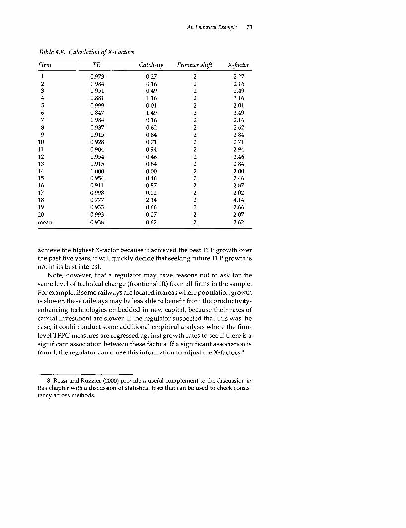
An Empirical Example 73

Table 4.8. Calculation of X-Factors

Firm TE Catch-up Frontier shift X-factor

1 0.973 0.27 2 2.272 0984 016 2 2163 0 951 0.49 2 2.494 0.881 1 16 2 3165 0 999 0 01 2 2.016 0 847 1 49 2 3.497 0 984 0.16 2 2.168 0.937 0.62 2 2 629 0.915 0.84 2 2 84

10 0 928 0.71 2 2 7111 0.904 0 94 2 2.9412 0.954 0 46 2 2.4613 0.915 0.84 2 2 8414 1.000 0.00 2 2 0015 0 954 0 46 2 2.4616 0.911 0 87 2 2.8717 0.998 0.02 2 2 0218 0 777 2 14 2 4.1419 0.933 0.66 2 2.6620 0.993 0.07 2 2 07mean 0 938 0.62 2 2 62

achieve the highest X-factor because it achieved the best TFP growth overthe past five years, it will quickly decide that seeking future TFP growth isnot in its best interest.

Note, however, that a regulator may have reasons not to ask for thesame level of technical change (frontier shift) from all firms in the sample.For example, if some railways are located in areas where population growthis slower, these railways may be less able to benefit from the productivity-enhancing technologies embedded in new capital, because their rates ofcapital investment are slower. If the regulator suspected that this was thecase, it could conduct some additional empirical analysis where the firm-level TFPC measures are regressed against growth rates to see if there is asignificant association between these factors. If a significant association isfound, the regulator could use this information to adjust the X-factors.A

8 Rossi and Ruzzier (2000) provide a useful complement to the discussion inthis chapter with a discussion of statistical tests that can be used to check consis-tency across methods.

5

Performance MeasurementIssues in Regulation

In the previous three chapters we assumed that the regulator had access togood quality data. This assumption allowed us to describe the various con-cepts and methods without the distraction of the many complexities of thereal world. In the remainder of this book we begin to relax this assumptionand discuss some of the many practical problems that regulators often face

In this chapter we discuss some of the issues that a regulator wouldneed to think about when attempting to use performance measures. Con-sider a standard problem a regulator will face. Say a new regulator mustmonitor the performance of an electricity distribution company, a sanita-tion company, a railway company, or a port. In some cases it may have alarge number of in-country comparators available, but in some other casesthe regulator may have to rely on an international comparison. This sectiontries to spell out the sequence of stages a regulator must go through beforeit can announce its estimate of the X that will apply to the firm it is sup-posed to monitor.

The first stage is to figure out what the regulator wants to do. Its maingoal is to get the firm it is supposed to monitor to produce at minimumcost, given the exogenous (and perhaps changing) environment it faces.The regulator will also look at various financial ratios as well as a safe-guard. In cases when it monitors several firms, the regulator may believethat some of the firms are more inefficient than others, and may thereforeconsider setting differential price caps in the first regulatory period, with aview to stimulating convergence toward the most efficient performancepossible by the end of the five-year period.

75

76 A Prtmer on Efficiency Measuremnettfor Utilities and Transport Regulators

Se~ling a Siingle X-lFacftor for AHi F7iEn

Assume that the regulator has access to some industry-level data and hlas

constructed a rough measure of industry TFP change for the last five yearsusing PIN methods. What are some of the potential pitfalls in setting the X-factor equal to this TFP measure?

o One could argue that with this approach, the consumer received allthe benefits of TFP growth, while the producers only eam normalprofits. Perhaps we should set a lower rate per year so that the firmsmake some extra dollars? But then at the end of five years these firmswill be earning a large extra profit per year. Do we take it all away atthe next cap setting? Or would we again be sending the wrong mes-

sage to the operators?o This rate may be too low if the monitored firms are inefficient rela-

tive to other firms in other countries. For example, we could look atthe United K<ingdom, where most of these rates have been calcu-lated at least once before. If our TFP rate is lower, the difference may

be an indication of what can be achieved when regulation is tight-ened and accumulated fat is cut from firms, especially in the earlyyears of the new regulatory regime. Furthermore, international com-parisons of TFP levels across different countries may also providesome indication of the relative productivity of the local industry.

o Much past and future TFP growth could be driven by improvementsembedded in new capital. If the industry is overcapitalized (excesscapacity) at present, the new regulatory environment may slow newinvestment. This may lead to lower TFP growth derived fTom em-bodied technical change. T'is may be the case in rail or ports, whereexcess investment has been the norm in many developing countries;however, in most developing countries the concern tends to beundercapitalization rather than overcapitalization.

o Investment may also be slow if demand growth is slow. New envi-ronmental laws may retard output growth in the next five years rela-tive to the previous period. This may also affect the average level ofenergy sold per customer, which could again influence the rate ofTFP growth.

o The position in the business cycle is important. If the next five yearsare part of the down cycle we might see an effect on demand growththat will flow through to TFP growth, so perhaps we should se. alower X factor.

Performianice Measurement Issues in Regulation 77

We have listed five examples here. There are a number of additionalones that have not been discussed. The key issue is to not use your perfor-mance measures in a vacuum. Always be on the look out for reasons why amodel that is applied to past data may not be directly applicable to thefuture.

For now, let us assume that we have considered all these issues and m2001 have set the industry X-factor at 2 percent per year. Now what hap-pens if in 2005 we find that the industry has actually achieved 3 percent peryear? Do we immediately remove the extra 5 percent (1 percent per year)the firms have built up and slap a new X-factor of 3 percent on them for the2006-10 period? This prospect may entice firms to play a game-such asusing extra inputs in the final year of the five-year price cap period so as todepress the measured TFP growth-which is not the incentive we want tointroduce. Rather than remove the 5 percent immediately, we could take itback gradually, say by adding a 1 percent "claw-back factor" to our base X-factor over the next five years. This means the industry can benefit frombeating the price cap for a longer period of time, but eventually it mustreturn to normal profit levels as would occur in a competitive industry.These are the types of judgment calls regulators must regularly make.i

Setting Firm-Specific X-Factors

The job is not over yet, because each of the firms will argue for specialtreatment. In particular, the least efficient firms are likely to try to convincethe regulator that they have good reasons for being less efficient. This meansthat the regulator should be able to assess the relative efficiency of each oneof the firms. This suggests two important questions, namely.

* What should be used to measure TFP differences between firms?* Once these measures have been calculated, how should they be used

in setting price caps?

Method choice depends partly on what data we have available and partlyon what we wish to do with the results. Assume that we have reasonabledata, for example, two to four years of data for each firm It can then esti-mate TFP for each firm using transitive PIN methods. The question then is,

1 One problem with this option is that it may still discourage firms from mno-vatmg in the latter years of the five-year price cap period One way in which onecan try to avoid this is to allow the firms to keep any supernormal profits for fiveyears from the year that they first earn them.

78 A Primer on Efficiency Measurement for Utilities and Tranzsport Regulators

are there any components of TFP that we may wish to exclude, for example,the effects of differences in output characteristics and environment, of scaleeconomies, or of allocative inefficiency? If we are interested in scale orallocative efficiency, we need to use a frontier method such as DEA or SfAto do this.

Which frontier method should we use? Here the opinions of variousefficiency measurement specialists tend to differ. We would argue that DEAmay not be the best method to use for a number of reasons. First, DEA doesnot account for possible noise and/or other interfering factors, which arelikely to be quite important in reforming or adjusting economies or sectors.Second, one must decide ahead of time the sign of the effect of each Z vari-able (environmental variable) upon efficiency so that we know if it is to beincluded as an input or as an output, as discussed in the next section. Third,one cannot determine the significance of the effect of the Z variables. Fourth,the shadow prices in DEA can vary a good deal across the sample, witnsome zero prices often found for some firms in the sample, which are diffi-cult to justify (see CRB for further discussion of the relative merits of DEAand SFA methods).

SFA is arguably a better method, but it also has potential problems, inparticular, the standard SFA method uses specific assumptions on residualskewness to separate inefficiency from measurement errors, which someeconometricians criticize. One alternative is to use OLS to estimate the SI'Amodel and then use expert judgment to adjus. the intercept parameter.2

However, such "expert judgment" may be susceptible to pressure fromvarious quarters. Perhaps the best approach to take is to estimate and re-port the standard SFA model and then discuss the degree to which the er-ror decomposition complies with expectations.

Now assume that the regulator has solved all the foregoing problemsand has measured all the components of the TFP differences between firms.Which bits should be removed? Practitioners usually argue that scale ef-fects should be excluded, because there are usually thought to be increas-ing returns to scale in utilities, and because size expansion is generally notpossible, at least in the short run. The issue of allocative inefficiency is quli ecomplex. When a regulator is faced with setting a price cap in a particularindustry for the first time, it often finds that some systematic allocativeinefficiency is present. If the industry was previously under rate of return

2. The two obvious possible extremes are OLS (no inefficiency exists) and cor-rected OLS (no noise exists).

Performance Measurement Issues in Regulation 79

regulation, a degree of overcapitalization may be apparent, that is, theAverch-Johnson effect (see Averch and Johnson 1962).

Alternatively, if the industry was previously government owned, theregulator may find excess labor and excess capital because of interferencefrom unions and politicians. Removing excess labor is not easy, but can beachieved over a five-year period. Reducing excess capital is not so easy(note that this has implications for both technical and allocative efficiency)Most capital in infrastructure is long-lived with the possible exception ofsome investments in the telecommunications sector. For example, if firm Ahas 50 percent excess capacity (that is, 50 percent higher than peak demandlevels) on a supply network for a particular city, then there are two obviousways it can address this situationr (a) wait for demand to increase, or (b)replace the asset with a smaller asset when the life of the asset has expired.When demand growth is flat and assets are relatively new, neither of theseoptions are available. The regulator could choose to write-down the valueof these assets, perhaps using an optimized replacement value approach,or alternatively, using the sale price of the firm if the firm was recently sold(and the market was not thin).

Another factor that may constrain a firm's ability to address an allocativeinefficiency problem in the short run is the degree to which the input ratiosare embodied in capital.3 For example, firm A may have a lot of capitalassets that are 20 years old and require more labor to maintain and operatethan the types of assets that are installed today. The old assets may havebeen the cost-minimizing choice 20 years ago given the capital and laborprices then, but now they are not. What can the firm do in the short run?

Overall, the existence of long-lived capital assets with limited resalepotential clearly makes the issue of allocative efficiency problematic. Thisis why some regulators have chosen to focus only on technical efficiency incomparing firms. In doing this they compare firms with similar input ra-tios (capital expenditures/operating expenditures) and thereby hope tomake more valid comparisons. However, this is not the end of the regula-tory challenge associated with efficiency measurement.

Now let us assume that the regulator has managed to measure technicalefficiency and finds out that some firms are not on the frontier. Take thecase where it finds that some firms are 80 percent efficient, while otherfirms are fully efficient (on the frontier). Now, should the regulator convertthis information into a firm-specific X-factor? Consider the case where the

3. This is a kind of putty-clay or vintage capital argument

80 A Primer on Efficiency Measurementfor Utilities and Tranisport Regulaitors

average TFP growth for that sector has been 3 percent. Does the regulatorset an X factor of 3 percent for the frontier firms and 7 percent (3 percent +4 percent) for the inefficient firms? This would ensure that all firmrs have anincentive to be equally efficient at the end of the next five-year period. Whymight this be a bad choice?

o For the regulator to insist that the frontier firms achieve 3 percentper year it must be assuming that the past TFP growth was due en-tirely to technical change. If part of it was due to technical efficiencyimprovement, say 0.5 percent, then it should perhaps only ask thefrontier firms to achieve 2.5 percent.

o If 0.5 percent of this past TFP growth was due to scale effects drivenby demand growth, and if the regulator believes that the new env i-ronmental laws will dampen demand growth, then perhaps it shouldremove another 0.5 percent from all X-factors.

However, at the beginning of the reform process, and in particular inpreparation for the first cap review, most regulators will not have sufficientdata to decompose the past 3 percent TFP change into these components,so let us assurme it is all due to technical change and continue. This meansthat the inefficient firms are stuck with a 7 percent catch-up componenLThis is quite tough. To make sure this is reasonable, the regulator mustwork with the operator to identify any environmental variables (Z vari-ables) and capital constraints we have not accounted for. This can reducethe X-factor imposed on some of the inefficient firms, but on a case by casebasis. This procedure must, of course, be carried out through public audi-ences to avoid the real risks of corruption.

Now, five years later, what does the regulator do? Let us assume thatsome firms have exceeded their X-factor while others have not reached it.How can the regulator set the new X-factors and maintain incentives? Forthose who exceeded the X-factor, should it take away all the gains immedi-ately or do so gradually over the next five-year period (with a firm-specificclaw-back factor)? What does it do with those that did not reach their X-factor? How does the regulator keep the pressure on them, still maintainincentives, and ensure that they do not go bankrupt? Whatever it decidesto do, it needs to clearly outline its strategy in the first year of the regula-tory period. Predictability and consistency are critical ingredients in anyincentive regulation structure. The introduction of uncertainty to the pro-cess is likely to dilute incentives.

Performance Measurement Issues in Regulation 81

Additional Comments

We have three additional important comments to make regarding the dis-cussion in this chapter as follows.

* We have treated operating expenditure and capital expenditure to-gether in this book. A number of regulators treat operating expendi-ture and capital expenditure separately, and only ask for operatingexpenditure productivity improvements while setting a "fair" rateof return on capital. This is the approach Green and Rodriguez-Pardina (1999) recommend. However, this approach can significantlydilute the incentive possibilities in CPI-X regulation. It restricts pos-sible cost savings to operating expenditure, which is often smallerthan capital expenditure in many infrastructure industries. Therewould also be an mcentive for firms to overcapitalize (the Averch-Johnson effect) to increase profits, which would mean that the regu-lator must then become involved in investment planning.Furthermore, such an approach would require careful selection ofproductivity measures. The regulator should take care in using stan-dard PIN TFP measures or standard efficiency measures derivedusing DEA or SFA, because they all include capital inputs in theirmeasures One option is to use an adjusted form of DEA where theefficiency measures only involve proportional reduction in the vari-able inputs, conditional on the levels of the fixed inputs (see Coelli,Rao, and Battese 1998, p. 172 for an example of a DEA model thatcan be used in this instance).

* We have not yet discussed the issue of the quality of service. Gener-ally the regulatory system requests that firms meet certain minimumquality standards, with substantial penalties for violations; however,note that any benchmarking involving international comparisonswould have to find some way of accounting for differences in qual-ity standards across countries. One way to address this problem isfor the regulatory system to explicitly define the way that qualitywill be taken into account in output measurement This implies thatregulators and utilities agree on the measurement of quality and onthe weighting procedure used (see Saal and Parker 2001 for an inter-esting case study in water utilities in the United Kingdom).

* The use of the CPI in a CPI-X price cap implicitly assumes that therate of increase in the prices the average consumer faces for food,

82 A Primer on Efficiency Measurenment for Utilities and Transport Regulators

housing, transport, leisure, and so on is equal to the rate of increasein the input prices paid by electricity distributors (on lines, trans-formers, wages, interest expenses, construction costs, equipment, andso forth). If this is not true, the X-factors need to be appropriatelyadjusted (see, for example, the discussion in Bernstein andSappington 1999, and for a real-life-related debate see, for instance,Office of Energy Regulation 2001).

6

Dealing with Data Concerns in Practice

Irrespective of which methodology the regulator chooses-PIN, SFA orDEA-it cannot avoid the first rule of empirical economics: garbage m =garbage out. The biggest hurdle that regulators will face is in obtainingenough data of sufficient quality to be able to conduct a robust, defensibleanalysis. A typical regulator will recruit an applied economist and give theeconomist the task of measuring efficiency in a particular network indus-try. Generally regulators give such people a strict deadline for completingthe task, perhaps three to six months. This means the economists must of-ten rely on secondary data sources. One of the typical main standard out-comes of a first empirical study will be a recommendation to improve thedata reporting standards for the regulated industry, so that in three to fiveyears time, when the next price cap review is due, the regulator will have amuch improved dataset available for analysis.' In the meantime, this chap-ter provides some guidance on how to use the data available, drawing fromexamples in the various sectors in which the authors have some experiencein measuring efficiency. 2 We begin with a discussion of input variables that

1 When setting reporting standards the regulator must keep in mind the costsfirms face m collecting such data and seek to minimize these costs where possible.In an ideal world, regulators from many countries would get together and define asubset of variables that they would all agree to collect so as to improve the qualityof international benchmarking studies. This would be especially valuable to smallcountries, where the sample sizes tend to be too small for the use of robust effi-ciency measurement techniques.

2 For an excellent introduction to data measurement issues mn performancestudies see chapter 10 m Morrison-Paul (1999). However, m readmg that chapterkeep in mind that the focus there is on sector-level data as opposed to firm-leveldata, between which some subtle differences exist

83

84 A Primer on Efficiency Measturemnentfor Utilities and Transport Regulators

could be used in an analysis of electricity distribution (for a comprehens-ivesurvey of recent analyses of productivity and efficiency in electricity trans-mission and distribution utilities see Jamasb and Pollitt 2000).

snpuls

The main categories of inputs are labor, capital, and other. To measure PINTFP indexes we require data on both quantities and prices for each inputcategory.

Labor

Labor can be divided into various categories, for example, unskilled, skilled,and management labor, but labor quantity is usually measured by a singleaggregate variable, such as the number of full-time equivalent employces

or aggregate hours worked. This is because of degrees of freedom limita-tions,3 or because labor is not consistently categorized across all firms. How-ever, keep in mind that this aggregation implicitly assumes uniform skilldistributions across firms. This is usually a reasonable assumption withinone country, but cross-country comparisons, say between the United Statesand India, could be problematic. One alternative is to measure labor quan-tity using total salary costs to attempt to account for differences in sklLIdistributions across firms; however, this will also be problematic if the rela-tive wage rates for the various categories do not reflect their relative

3. Degrees of freedom is the term used in regression analysis to relate the quan-tity of information we put into a model (observations) to the quantity of informa-tion we want to take out of it (the estimated parameters). Large degrees of freedomare good and small degrees of freedom are a worry. In regression analysis the ex-treme case is zero degrees of freedom, when the number of observations equals t'nenumber of parameters. In this case all data points will lie on the fitted lne. Therewill be no deviations from the line, and hence in a production or cost frontier thcrewill be no (measured) inefficiency. This is good news for firms and bad news forregulators A similar thing happens in DEA, although no parameter estimates areexplicitly involved For example, we note that the addition of an extra variable to aDEA model, with the sample size held fixed, cannot cause the efficiency score ofany firm to fall, but can, and often does, cause it to rise Similarly, the removal of anobservation from a sample cannot cause the efficiency score of any remaining firmto fall, but can cause it to rise. Refer to Zhang and Bartels (1998) for a good illustra-tion of the sample size effect in electricity distribution using data from Australia,New Zealand, and Sweden.

Dealing with Data Concerns in Practice 85

marginal products, which is almost impossible to verify, or if the wagerates differ between firms because of geographical and other factors (seethe discussion later about selecting suitable price deflators).

The price of labor can be measured in various ways. If the quantity ismeasured using the number of employees or hours worked, then a com-mon approach is to measure the price of labor of each firm as the total laborcosts divided by the quantity measure. This implicit labor price will pickup geographlcal differences m wages, assuming constant labor quality acrossfirms; however, if labor quality (skill mix and so on) is not constant acrossfirms, the quantity and price measures will be biased.

Capital

A discussion of the capital input could easily fill an entire book. To beginwith consider the search for a measure of the quantity of capital, that is,what is the potential service flow from the capital?4 As with labor, we canuse physical quantities or monetary proxies. Physical measures are oftenused in international comparisons because of the many problems encoun-tered in obtaining consistent capital valuations across different countries.These issues are discussed further later.

The main capital items in electricity distribution are lines and trans-formers, in ports they include the docks and the superstructure, in rail thetracks and rolling stock, and in water the pipes and the treatment stations.Other capital items would be buildings, vehicles, small machinery, com-puters, and so forth. However, each sector always has a couple of catego-ries that are by far the biggest capital categories in terms of their annualizedcontributions to costs, and most of these inputs are far from being a ho-mogenous commodity. For instance, in electricity distribution lines may beoverhead (on poles) or underground. Poles may be wooden, concrete, orsteel. The lines may be low or medium voltage (high-voltage lines areassumed to be part of the transmission network, not the distribution

4. Some people argue that we should try to account for capacity utilization mthe capital measure. We would tend to argue that no adjustment should be madefor capacity utilization, especially when dealing with cross-sectional data (see thelater discussion of optimuzed capital measures). However, when looking at paneldata and measuring TFP growth over time, one should keep the general effect ofthe macro-economy in mmd when assessmg the past performance of an mdustryand its likely future productivity growth prospects.

86 A Primer onl Efficienicy Measurementfor Utilties and Transport Regulatorb

network).5 The number of wires also differs across different parts of thenetwork. In empirical studies the lines capital item is often proxied by asingle variable, such as the length (kilometers) of network or the length ofnetwork weighted by voltage. The "braveness" of this approximation willvary from sample to sample. Transformers can also be of various sizes andtypes. Transformer capital is often proxied by the total sum of name-platetransformer capacity in megavolt amps. The validity of aggregatingtransformers of differing sizes, and hence costs per megavolt amp, is a po-tential criticism of this approach; however, there are fewer potential prob-lems than with the lines measure, which is much more heterogeneous.

Given these problems with physical capital measures, using a monetaryproxy for capital is tempting. With it we can aggregate all these capitalitems together to form a single capital variable so as to minimize the num-ber of variables in our model and thus conserve degrees of freedom. Beforewe discuss how this can be done, note that in a DEA analysis there areadvantages to having separate measures of the various types of capital in-puts. Returning to the electricity example, this occurs when different firmsdeliver electricity to geographical areas with different population densi-ties. In this instance a DEA model with separate lines and transformer mea-sures will tend to pick out better peers (benchmark partners), because firmsin sparsely populated areas will have relatively higher line to transformerratios, and thus peer sets will have similar population densities. 6

The construction of a value measure of capital quantity is a complexissue, and because of this we have devoted the appendix to the topic. Readthis appendix carefully before collecting data for capital measurement. Afirm's accounting records are an obvious source of information on capitalvalues; however the collection process holds many traps for the unwary,including

o Divergence between accounting and economic definitions of depre-ciation

o Effects of inflationo Effects of lumpy capital investment

5. For example, in Australia 77 kilovolts is generally used to define the bound-ary between transmission and distribution networks.

6. Firms in sparsely populated areas also tend to have low labor to capital andother inputs to capital ratios, and hence this nice, automatic peer selection effectwill still happen to some extent, even if you only have a single aggregate measureof capital.

Dealing with Data Concerns in Practice 87

* Different firms using differing depreciation schedules* Different tax rules and inflation rates in international comparison

data.

This leads us to recommend the use of undepreciated replacement val-ues as a proxy for capital quantity in the appendix, but if these are notavailable, we also discuss the relative merits of various second-best mea-sures. Furthermore, we discuss various ways of calculating the user cost ofcapital, and thus the implicit price of capital.

Other Inputs

The other inputs variable is a catch-all category containng inputs other thanlabor and capital. It will contain mostly office and vehicle expenses (power,fuel, materials, services, and so on) The contribution of these individual itemsto total costs is generally small relative to capital and labor, and thereforethey often do not warrant separate variables, though in some cases, for ex-ample, for rail and bus companies, the fuel category may be sufficiently largeto warrant a separate mput measure. Furthermore, different firms tend tocategorize their records differently, making consistent cross-firm compari-sons difficult unless regulatory data forms list specific categones.

One item that is making an increasingly large contribution to the otherinputs category in many firms these days is outsourcing. When significantoutsourcing of maintenance contracts occurs, the relevance of the distinc-tion between the labor and other categories begin to blur. In such situationsregulators may choose to specify a variable inputs category that containsall noncapital costs, mcluding labor costs. Note, however, that the validuse of value measures of capital, labor, or other inputs hinges on the as-sumption that all firms face the same prices. If this is not true, the regulatormust fmd suitable price deflators. This obviously becomes a significant is-sue when making inter-temporal and international comparisons

Allocation of Overhead Costs and Other Issues

In several instances some costs have to be allocated across activities. First,in many sectors firms have various activities, not all of them regulated, andthus you often need to allocate various overhead costs, such as head officecosts, to different activities of the same firm. For example, as well as beinginvolved in electricity distribution, an electricity firm may also be involvedin capital construction (generally of its own network), retail, and consultancy

88 A Priner on Efficiency Measurement for Utilities and Transport Regulators

activities. When collecting data the regulator must devise a rule for allocat-ing overheads that is fair to different types of firms and apply this ruleuniformly across all firms.

Second, the regulator must judge how to draw the line between capitalexpenditure and maintenance expenditure. Consider again the example ofelectricity distributors. Is the replacement of insulators maintenance or capi-tal investment? Is the replacement of wooden poles maintenance or invest-ment? One could argue that pole replacement is clearly investment, yet anumber of Australian electricity distributors list it on their books as main-tenance. The maintenance/capital line can be drawn in any number ofplaces, and the key issue is to draw it in the same place for all firms. Earlyand clear specification of such distinctions will reduce the cost of regula-tory data collection and improve the quality of the results obtained in sub-sequent efficiency analyses.

A related, and more complex, issue is how to relate the maintenanceregime in a firm to the expected life of an asset. Generally we insist onassuming the same asset lives for all firms in the sample. This is either doneexplicitly by replacement cost depreciation calculations, implicitly by us-ing replacement cost as a proxy for service flow, or by using physical capi-tal measures such as lines and transformers. Consider the example of twofirms, A and B. Firm A does twice as much maintenance as firm B, andtherefore can arguably expect its assets to have a longer expected life. How-ever, if we apply the same expected asset lives to both firms, firm A willappear to be more inefficient than it actually is. Could this problem be amajor issue in a dataset? In industrial countries the maintenance proce-dures are fairly uniform, but in some developing countries this could be anissue warranting careful attention.

Finally, one of the most obvious questions in a network industry iswhether the network is an input or an output. This is one of the main sourcesof debate at meetings of regulators, distributors, and efficiency measure-ment consultants. Some representatives of electricity distribution compa-nies have been heard to state that their job is to have the network availableto carry the electricity, and that the amount of electricity carried along aparticular line (10 percent or 90 percent of capacity) will not affect the costof maintaining the line. However, engineers would be unlikely to agreewith this observation. Indeed, many (if not all) published analyses of tech-nical efficiency in electricity distribution include network length (or somerelated variable) as an input and not as an output.

When constructing a model for regulation purposes there is an obviousdanger involved in including network length as an output variable to

Dealing with Data Concerns in Practice 89

account for density issues. It will mtroduce perverse incentives by encour-agmg expansion of the network solely to improve a firm's efficiency score.The issue of network density is better dealt with in other ways. As alreadynoted, the inclusion of separate measures of transformers and lines willtend to ensure that firms facing similar population densities are bench-marked against each other. Another option, also mentioned earlier, is tohold the capital input fixed when measuring efficiency. Third, if the regula-tor is still concerned it can define a range of population density measuresand use these to see if the efficiency scores are systematically related tothese factors.

Outputs

Output measures are even more complex than input measures. The obvi-ous output measure is the quantity of electricity, of water, or of passengerstransported. However, the costs involved in delivering E units of mediumvoltage electricity to one customer are clearly not the same as supplying E/1,000 units of low voltage electricity to each of 1,000 households, as is, partlyor fully, reflected in the differential tariffs charged. Thus we seek some wayof differentiating between customer types, namely, high and low volume,residential and business customers, and so on.

The most common measures of rail outputs are passenger kilometersand tonne kilometers of freight. These measures will clearly be imperfect.Some studies argue that these measures of output are heavily influencedby demand conditions, which may or may not be controllable. They there-fore suggest using supply-based output measures, such as the number ofseat kilometers, irrespective of whether or not they are occupied. This ap-proach may be problematic for two reasons. First, running almost emptytrains will clearly cost less in terms of fuel, ticketing, and cleaning coststhan running almost full trains. Second, a model with a supply-based out-put measure may introduce perverse incentives for the companies to intro-duce services in areas of low demand at off-peak times so as to improvemeasured efficiency.

The relevance of the multiplicity of outputs explains why in many stud-ies the authors use at least two output variables: electricity, gas, or waterdelivered and number of customers; or number of passengers and tons offreight; or number of containers. If the regulator has degrees of freedomand data to play with, then it can divide these variables into smaller cat-egories. This has the advantage of allowing the selection of better peer firmsin the efficiency comparisons.

90 A Primer on Efficiency Measurement for Utilities and Transport Regnlators

In some cases the relative "pealciness" of demand can be a big issue.This is particularly true when comparing firms across diverse climatic re-gions or regions with different types of business activities. The load profile(the demand) can differ substantially between times of the day and be-tween seasons and do so differently in different regions. The networks mustbe designed to deal with these peaks. Thus the regulator may also includea measure of peak supply (along with total supply and customer numbervariables) to account for this issue.

Some studies treat pollution as a "bad" output. This can sometimes bean important issue. For example, the installation of scrubbers to reduceemissions in power plants can be extremely costly, and can make TFP changemeasures appear to be low. The inclusion of bad outputs in TFP and effi-ciency studies is the subject of a number of recent papers, for example, HFreand others (1989).

Quality

The discussion of output measures did not consider certain possible qual-ity differences. Reliability of supply is clearly the big quality issue in elec-tricity distribution. Typical quality measures in industrial countries includeaverage length of supply interruption per customer per year, delays, can-cellations, and average time taken to restore supply when it has been inte-r-rupted. Collecting comparable data about supply reliability is generallydifficult using existing data records because of variation in the definitionsof the measures used, both between firms in some countries, and in par-ticular between firms in different countries. lDeveloping an internationallycomparable set of definitions of reliability measures should be a priorityfor all regulators.

One problem with reliability measures (and the demand for output to alesser extent) is that they can be substantially influenced by environmentalevents. For example, an unusually bad cyclone in one year in one geographi-cal area may make electricity supply reliability figures look quite bad forthe firms involved. Similarly, a particularly harsh winter or hot summercan cause the amount of electricity supplied by a firm to look quite good insuch years. These issues indicate some of the dangers involved in using asingle cross-section of data to evaluate relative performance.

In addition, a quality variable that needs to be taken into account is .hetechnical quality of the service. The distribution of water and electricitywill invariably result in losses. The design and maintenance of the networkwill determine how much is lost. Some studies include these losses as a

Dealing with Data Concerns in Practice 91

variable, some include the cost of losses in the other mputs category, while

other studies simply ignore it. This is one of the many judgment calls theregulator has to make.

Quality variables differ between industries. In rail the reliabilhty of sup-ply, that is, timeliness, is important, but safety, degree of overcrowding,frequency of services, cleanliness, and comfort of passengers are also im-

portant aspects of the quality of service. In the case of freight transport, thegoods arrivmg undamaged is an important quality measure.

Sometimes regulators can account for some aspects of quality by care-fully specifying the output measure(s). For example, two rail firms mayoffer quite different qualities of service. Firm A may provide large roomyseats, food and drinks served at passengers' seats, and so on, while firm Bmay not offer this degree of service. If this difference is reflected in theticket prices, then a revenue measure may be a better proxy for outputquantity than the traditional passenger-kilometers measure. However, ifthe prices differ for other reasons, such as local subsidies, the revenue mea-sure wliU be biased.

Quality issues can, in some cases, be left out of the model, for example,when the regulator is analyzing a group of firms from one country whereuniform minimum standards apply to all firms. The regulator can imposesignificant penalties for violating these standards, and then deal with TFPand pricing issues separately. However, when comparing firms that facedifferent standards, perhaps because they are from different countries,quality will have to be considered as part of the TFP comparison. If de-grees of freedom allow, and if a consistent measure of quality is available,regulators can include a quality variable; however, if it expects the effectto be limited to a few firms, or if degrees of freedom are tight, the bestapproach might be to omit the quality variable, and then ask the firms todiscuss their individual situation with the regulator if they believe theyhave a case.

Quality can sometimes be an important issue in TFP measurement acrosstime. For example, Saal and Parker's (2000) study of TFP change m thewater sector m the United Kingdom showed that TFP change has been ex-tremely slow in recent years, but that quality has improved significantlybecause of the large increases in minimum standards, which have incurredsignificant costs. Thus the use of unadjusted TFP change measures fromthis period would understate the potential TFP improvements (given thatthe quality standards are not raised again m the coming period). The Saaland Parker (2000) study suggested the use of quality-adjusted output mea-sures to account for this effect.

92 A Primer on Efficiency Measurement for Utilities and Transport Regulators

lEnvironment

Environmental variables, which efficiency studies often refer to as Z vari-ables, are elements of the physical, cultural, or institutional environmcntthat can affect efficiency. Like traditional input and output variables, thesevariables are not under the control of managers. The important variables inthis category tend to be just as sector specific as quality variables. mne envi-ronment for electricity is often dominated by, but not restricted to, popula-tion density, climatic, and geographic variables. The main environmentalfactors that can affect railways are density, topography, average haul length,average load, and government policy. In some cases the environment mayalso include information about the regulatory environment and other non-physical items. Examples of typical environmental effects include low popu-lation density leading to higher costs, storms that cause fallen trees to bringdown lines or stop trains, and rugged topography that makes access formaintenance tearns costly

Defining suitable measures can be tough. Even population density canbe problematic, because an area with one large city and a big unpopulatedarea such as a desert can have the same population density as an area withmany evenly scattered small and medium towns. These two configurationrswill clearly require different network resources.

With little effort a regulator can quickly obtain a long list of possioleenvironmental variables to include in any model. Each firm will argue forthe inclusion of the variables that will make it look better. The regula.ormust limit these variables to the smallest set possible, so as to control de-grees of freedom. It should include only those variables that are likely tohave a large effect upon a number of firms. In the case when a Z variable islikely to affect only one or two firms, the regulator can invite the firmsinvolved to make a case for the amount by which it should adjust thleirefficiency score to account for this.

lPices

One of the main challenges is to obtain good input price information.7 Giventhat price x quantity = cost, we need to find at least two of these three item's

7. The regulator can also obtain output price information and look at theallocative efficiency associated with the output rnix, and hence also consider pro,itefficiency and/or revenue efficiency However, in infrastructure industries the oui-put quantities and mix are rarely under the control of the firm, and thus thesestudies usually focus on technical efficiency and/or cost efficiency.

Dealing with Data Concerns in Practice 93

for each input. Because of data availability issues, the following data areoften used:

* Labor: quantity and cost data obtained from each firm8

* Capital: replacement cost data constructed for each firm and pricedata based on capital price index numbers and interest rates obtainedfrom a secondary source9

* Other: cost data obtained from each firm and price data based onindex numbers obtained from a secondary source, such as the na-tional statistics bureau.

Note that when an input quantity has been measured in value termsand the regulator believes that prices are constant across firms, for instance,when it has cross-sectional data and expects no geographical price varia-tion, the price of one unit of this input is simply 1.

Depending on the method chosen, a lack of pnce variation between firmscan be a problem. The regulator must carefully distinguish between thesituation of no price variation between firms because they face the sameprices, and the situation where it has no measure of price variation be-tween firms when they do face different prices. Assuming the first case,using cost minimization DEA does not present a major problem and it canbe carried out with a single price for all firms if need be.

If the regulator has no price information, but believes that all firms facethe same prices, it can estimate a cost frontier, where total cost is a functionof output quantities. 1 0 This will provide cost efficiency scores, but the regu-lator will not be able to decompose these into technical and allocative compo-nents. By contrast, if it has estimated such a function assuming uniformprices when this is not the case in reality, it may then end up labeling a firmas cost inefficient when it is actually efficient, but simply faces higher prices.

8 The imphcit labor price obtained by dividing the total wage bill by the totalnumber of employees can, in some cases, pnmarily indicate differences in laborforce composition across firms rather than true geographical price variation

9. Given that the user cost of capital consists of depreciation and opportunitycost, it will only vary between firms if they face different capital procurement costsand/or interest rates. This becomes more likely when dealmg with panel data and/or international comparisons.

10. The dependent variable could be total costs, including both fixed (capital)costs and variable costs, or it could be just variable costs In this latter case theregulator should include one or more variables reflecting the quantity of fixed capitalas regressors.

94 A Primer on Efficiency Measurementfor Utilities and Transport Regulators

PaneR l Data and Hntemationall CGmypzzs-sL

So far the data discussion in this chapter has not involved issues associatedwith time variation. What if the regulator actually has a panel of data cov-ering several firms over several years? Access to panel data is clearly agood thing. We have already discussed the dangers of looking at just oneyear of data, where one weather event can have a major influence on somefirms, or where a simple model may label a sensible long-term investmentstrategy as inefficient in the short run. With panel data we can obtain infor-mation on TFP growth and decompose it into components: technical change(shifts in the frontier), technical efficiency change (catch-up), and scale effi-ciency change.

Panel data provides no new data-related problems when only physicalmeasures with consistent definitions are used; however, almost all studiesinvolve the use of at least some value measures. For example, the use of avalue measure of the other inputs variable, such as office and vehicle ex-penses, is usually unavoidable. Whenever we use value measures fromdifferent years we need to account for the effects of price inflation. Remem-ber that we want the input measure to be a proxy for the physical inputquantity. The choice of a good price deflator is crucial. Whenever possible,the regulator should try to avoid the use of the CPI. The average change inthe prices of groceries, clothing, residential housing, vacations, and house-hold furniture and electrical goods is usually a poor measure of the aver-age price change in office and vehicle expenses in the electricity industry(or the price of transformers and electricity poles, engineers' wage rates,and so on). In an ideal situation the regulator will have detailed price in-dexes for the various input categories in the electricity industry. A second-best strategy is to use general price indexes for labor, capital, and materialsin manufacturing industries, which are usually available from the nationalstatistics bureau in each country. The CPI should be used as a last resort.

Finally, comparing a local monopoly with monopolies in comparablecountries may be interesting. This is a panel data problem, but a muchmore complex one. Constructing datasets for international comparisons ofinfrastructure firms is a messy business. The data collected in different coun-tries is generally different. This is for various reasons: historical, environ-mental, regulatory, and so on. The task is to collect data that is (a) relevantto local issues, (b) permits international comparison work, and (c) does notput too great an administrative burden on the firms.

Many countries collect quite similar information, but slight variationsin definitions lead to comparability problems. For example, the voltage level

Dealhng with Data Conicerns in Practice 95

used to distinguish transmission lines from distribution lines differs be-tween certain countries; the division of customers into small, medium, andlarge categories is based on a variety of annual consumption levels in dif-ferent countries; and so on. The development of an internationally consis-tent set of reporting standards for the principal network industries wouldbe a significant benefit to regulators around the world.

Finally, one of the key reasons for including international firms in theperformance measurement analysis is to increase the chance that the regu-lator has included best practice firms in the database. If the regulator'sdatabase is limited to a handful of local firms that are all equally mediocre,then the best practice level in its analysis is likely to be a long way fromtrue best practice. Including data from other countries' firms will no doubtincrease the complexity of an analysis, but the potential benefits can faroutweigh the costs.

Additional Issues

One question that has generated some debate in the efficiency literature iswhether environment and quality variables should be included directly inthe production model, or whether regulators should only include the tradi-tional input and output variables in the model, and then relate the effi-ciency scores obtained to these other variables in some type of second-stageanalysis. A complicating issue is that the boundary between the variablegroups is rather fuzzy. Is demand peakiness an output or an environmen-tal issue? Is reliability of supply a quality issue or an output? The advan-tage of including all the variables in the production model directly is that itcan help the regulator identify more appropriate peer sets. The disadvan-tage is that the regulator may identify no peers at all, because all firms willbe unique, and hence lie on the efficiency frontier.

The inclusion of nontraditional variables into a production frontier re-quires some careful mterpretation of the resulting efficiency scores. Forexample, if the regulator included an average winter temperature variablein an electricity distribution model to account for possibly higher mainte-nance costs in extremely cold climates, then the implication is that the in-tercept of the frontier now differs according to the temperature. This bringsus to the issue of net versus gross efficiency measures, discussed by Coelli,Perelman, and Romano (1999) in the context of international airlines. Con-sidering the temperature in our electricity distribution example, the regu-lator will obtain technical efficiency measures, which are net of the effect oftemperature, if it includes the electricity variable in the model. However, if

96 A Primer on Efficiency Measurement for Utilities and Transport Regulators

it omits the temperature variable, it obtains gross technical efficiency scores(inclusive of any temperature influence). The key issue here is to recognizethat deviations from the frontier can be due to two groups of factors: thoseunder the control of management and those not under management's con-trol. At the end of the day the regulator needs to disentangle these twoeffects.

One issue that arises, irrespective of the methodology chosen, is the ex-istence of outliers. The three main reasons for outliers are (a) typographicalerrors; (b) invalid observations, for example, an electricity transmissioncompany in a sample of electricity distributors; or (c) unusual observa-tions, for instance, an electricity distributor serving an area with a low pop-a-lation density. The regulator should not simply drop outliers based on somearbitrary criteria. It should correct the typographical errors (if possible),drop the invalid observations, and keep a close eye on the unusual obser-vations as the analysis progresses.

Identifying outliers is a time-consuming but essential task. The follow-ing are some useful ways to approach the task. The regulator should

1. Check its dataset with alternative sources if possible. If it has datafrom a regulatory return form, it should try cross-checking whatvariables it can with annual reports or some other alternative datasource.

2. Check its data for internal consistency. For example, if it has costdata it should ensure that the individual cost components add up tothe total cost figure for each firm.

3. Look for zeros in the data, and then ask if ihey are sensible. Is sup-plying electricity with zero kilometers of lines a possibility?

4. Look at the sample means, standard deviations, minimums, maxi-mums, and plots of all variables. Are a few data points situated along way from the others? If so, why is this so?

5. Construct ratios of each variable over every other variable and re-peat the previous exercise. Do some firms have more employees thancustomers? Does this make sense? Note that some partial productiv-ity ratios can be reported in the final paper as well. The partial ratiosoften provide useful complementary information and can help cx-plain the factors underlying the efficiency scores obtained from theother more comprehensive, and therefore more complex, methods.

6. Estimate some rough Cobb-Douglas OLS production, cost, and/ordistance functions before estimating the final DEA or SFA model;look for large residuals and influential observations; and study them

Dealing wVIth Data Concerns in Practice 97

carefully. Often the regulator witl find that some observations thatlooked like outliers in the partial ratios look alright now, while theOLS residuals may identify some potential outliers that did not showup in the partial ratios.

Clearly, positive outliers can influence a deterministic method like DEA.One observation with an output measure that is 20 percent higher than itshould be can have a nontrivial (negative) influence on the efficiency scoresof many firms in the sample. In DEA counting the number of times eachfrontier firm is listed as a peer for another firm is a good idea. For example,if the regulator finds that one firm is being referenced as a peer by half thesample, this may be cause for some concern. It needs to take a close look atthis firm. It may even try dropping this firm to look at the sensitivity of theresults to its inclusion.

While only positive outliers affect DEA, both negative and positive out-liers will affect SFA and OLS, thus the regulator should look carefully forboth types of outliers when using the parametric methods. Furthermore, itshould always assume that the data contain some errors. Finding errors indata that have already been carefully checked by the company accountant,the auditor, the regulator's office, and the research assistant of the econo-mist doing the actual work is not uncommon.

In addition, one of the fundamental questions is determining the cor-rect number of variables to include in the model. This question must beasked when constructing any econometric model Consider, for example,the case of a rail study. Comimg up with a long list of outputs, inputs, andenvironmental variables would not be difficult. Outputs could includefreight and passenger trips. Freight could be divided mto bulk and nonbulk,and passenger trips could be divided into short and long trips, with longtrips divided into fast train and regular train services. The main inputscould include labor, fuel, length of lines, number of stations, number oflocomotives, and number of passenger and freight cars. Lines could be di-vided into fast lines and regular lines, electrified and nonelectrified lImes.Environmental variables could include the steepness of the terrain, popu-lation density, and so on. Already we have 16 possible variables, and wecould easily think of some more. In a translog model this would produce ahuge number of parameters to estimate, most likely more than the numberof available observations. Our model estimates would be poorly estimated.We must strike a balance by aggregating some variables and omitting oth-ers. These decisions should be driven by a combination of prior knowledgeof the industry and standard statistical tests. At the end of the day we must

98 A Primer on Efficiency Measurementfor Utilities and Tranisport Regulators

accept that our model will be imperfect. If some firms believe the modeldoes not account for their situation, then they must make their case knownto the regulator. For example, in a study of European railways Switzerlandcould make a case for higher fuel costs because of its steeper terrain if themodel does not include a terrain variable.

A related issue is that in some cases constructing a model for the wholefirm may be too difficult, because each firm may be involved in variousactivities. In this case the best approach may be to segment the data intoactivities and then run a model for each activity, as the Office of WaterServices does for U.K. water companies. For example, a sample of watercompanies firms' activities may include water collection (dams, bores, andso on), water distribution, sewerage pipes, and/or sewerage treatment, andsome firms may only be involved in a subset of these activities. Further-more, the construction of a single model to deal properly with all the maininput and output variables may be impossible, given limited numbers ofobservations. Thus constructing separate models for each activity may bethe only sensible way to proceed, but the regulator must have good datathat permit the identification of inputs and outputs for each activity (in-cluding the allocation of overheads), and must also be confident that sepa-rability between activities is a reasonable assumption.

7

Choice of Methodology

The selection of the best methodology to use in a particular application canbe influenced by a number of factors, including

* The availability of data* The likely importance of data noise* The intended use of the results.

Data availability is always an issue. If you require a measure of TFPgrowth over time, then you must use whatever data are available. In somecases the availability of firm-level panel data will be extremely limited,and in such instances you may be forced to use aggregate (industry-level)time series data. In this case the methodology choice is essentially limitedto the use of PIN methods such as Tornqvist or Fisher indexes.

Alternative econometric approaches, such as an OLS cost function basedon time series data, are generally not recommended. To get reasonable de-grees of freedom, you need a lengthy time series of data that is either notavailable or extends back to a period when technologies and/or data defi-nitions differed significantly. For example, the number of free parametersin a translog cost function with two outputs, one fixed input, two variableinput prices, and a time trend variable, a fairly basic list of variables, isequal to N(N + 1)/2 = 6(6 + 1)/2 = 21, with symmetry and homogeneityrestrictions imposed. Thus to get the often quoted figure of 30 degrees offreedom or more, you require at least 51 years of data, which would takeyou back to the 1940s.

The inclusion of data points from more than one country may have abearing on method choice. Obtaining consistent price and cost data acrossdifferent countries can sometimes be difficult. Collecting consistent physi-cal input and output data may be less problematic. This may encourage

99

100 A Primer on Efficiency Measutrenientfor Utilties and Transport Regulators

you to choose a primal approach using DEA or SrA over a PIN approach ora cost frontier approach using SFA, but keep in mind that these methodswill not capture the effects of allocative efficiency changes.

The amount of suspected data noise can influence the choice of meth-odology. SFA attempts to account for noise, while DEA assumes it does notexist. Hence if you suspect that your data are of low quality, you may de-cide to steer away from DEA. However, you also need to take care withSFA. The standard maximum likelihood approach uses the skewness in theresiduals to disentangle noise and inefficiency, thus outliers can influencethis decomposition. A few large, positive residuals may convince the methodthat most of the error term is due to noise, while a few large, negative re-siduals may convince it that most of the error term is due to inefficiency.'One alternative is to estimate the SFA frontier using some variant of cor-rected OLS, using expert knowledge to adjust the intercept. However, thedegree of such adjustments will clearly be a target for lobbying.

The degree of confidence you can have in efficiency scores and rankingsis clearly important. Can we produce confidence intervals for our predictedefficiency scores? The answer is a qualified yes. See, for example, Kim andSchmidt (2000) for a review of the various methods that can be used inparametric models and Simar and Wilson (2000) for a discussion of thlebootstrap method applied to DEA models. However, most of these meth-ods are quite complex and have yet to become mainstream in the appliedliterature. Our advice is to have a look at these methods and judge for youir-self whether they are feasible for you to complete within your timeconstraints.

The way in which you intend to use the results of your analysis iAillobviously have a bearing on the method chosen. Are you seeking a single,industry-wide TFP measure, or do you wish to set differential X-factors foreach firm? A PIN analysis using annual aggregate data will provide anindustry-wide TFP growth measure, but if you seek firm-specific X-factorsthen you may be interested in some form of frontier analysis, that is, applyDEA or SFA to cross-sectional or panel data.

One factor to keep in mind when assessing a firm's abilit'y to achieve aparticular X-factor is to look at the amount of new investment in capital

1. For example, some empirical studies have estimated separate SFA modelsfor each cross-section in a panel dataset and noted that the percentage of the errorterm attributed to inefficiency can jump around from year to year in an unsatisfac-tory way, being near 0 in one year and near 100 percent in the next.

Choice of Methodology 101

that is planned for that firm over the next regulatory period (usually fiveyears). The point is that technical change can be both embodied and disem-bodied, and a firm that has significant investment plans, either because ofdemand growth or because of replacement of existing capital, will find thatTFP growth is easier to achieve than a firm that has less planned invest-ment activity.

One important issue to keep in mind in method selection is that differ-ent methods can yield different answers. For example, Ferrier and Lovell(1990), in their study of banking efficiency, found that DEA and SFA scoresderived from the same dataset were essentially uncorrelated. However, thisis not always the case For example, in a study of European railways, Coelliand Perelman (1999) found a strong correlation between the scores obtainedusing three different methods. Either way, if possible you should apply asmany methods as possible to minimize the possible impact of method se-lection on the results.

One potentially large source of differences in measures of TFP growth isthat due to differences between shadow prices and market prices. Moststandard applications of PIN methods use market prices as weights, whileprimal methods, such as DEA and SFA production frontiers, implicitly useshadow prices to weight the multiple inputs and outputs. Thus if you usepanel data from periods when cost minimization was not the firms' objec-tive, then the shadow prices can deviate from market prices, and the result-ing TFP measures will differ from those obtained using PIN TFP growthmeasures constructed using market price information (see, for example,the analysis of Australian electricity generation in Coelli 2002, where thedifference obtained is substantial).

An important question to ask when selecting a TFP measurement methodis whether you wish to include allocative efficiency in the TFP measure? Anumber of authors define TFP as a purely technical measure, for example,Fare and others (1994) measure TFP growth using DEA methods and de-compose it into technical change, technical efficiency change, and scale ef-ficiency change components, but make no mention of allocative efficiency.As Coelli (2002) noted, many of the most widely cited papers on TFP donot include allocative efficiency in their TFP definitions. However, if weuse PIN methods or estimate a cost frontier using OLS or SFA, we will tendto pick up the effects of changes in allocative efficiency in our TFP measure.The regulatory implications of this observation are interesting. The effectsof previous regulatory regimes may have left firms with considerable scopefor cost savings through allocative efficiency improvement. For example,privately-owned U.S. electricity distributors, which previously faced rate

102 A Prinmer on Efficwency Measuremeentfor Utilities and Transport Regulators

of return regulation, may have considerable excess capital capacity tha,Lthey can slowly reduce through depreciation or demand growth, whileAustralian electricity distributors showed that they have been able to shedsignificant amounts of excess labor in the 1980s andl990s, a carryover fromyears of government ownership and strong labor unions.

Thus two obvious regulatory errors are possible. Consider the case wheremeasured TFP growth has been 2 percent per year excluding allocative ef-ficiency changes and 4 percent per year including it. Now if most of theallocative improvement has been made already, then insisting that firmscan achieve the 4 percent growth over the next five years may be harsh.Alternatively, if more allocative slack remains to be corrected, then request-mg only 2 percent annual TFP growth may be too lenient. At the end of theday, regulators are interested in the degree to which firms could be reason-ably expected to reduce costs, in real terms. Thus they should be interestedin allocative efficiency, but should also think carefully about the foregoingissues. In a situation where correctly implemented incentive regulation hasalready been in place for a number of years, we would expect the vastmajority of TFP growth to be due to technical change, with technical ei'.i-ciency change and allocative efficiency change playing minor roles. There-fore the selection of a TFP measurement methodology should have muchless influence on the results obtained in that si,uation.

The orientation of a model can influence the results obtained. For ex-ample, in DEA or in SFA distance functions you can choose either an inputorientation or an output orientation for the model. This is usually done onthe basis of which set of variables, inputs or outputs, the firm has mostcontrol over. In the case of utilities, firms often have more control over in-puts, because these firms must usually supply the level of output (electric-ity, water, and so on) that the public demands, and have little influenceover output levels. When the technology is CRS, the choice or orientationwill have no effect on the measured levels of TFP or its decomposition;however, when CRS does not hold, which is generally the case, the contri-bution of scale efficiency in the decomposition can be affected by the orien-tation. The following results apply. Under increasing returns to scale, theinput-oriented scale efficiency measure will be smaller than the output-oriented scale efficiency measure, while for decreasing returns to scale ;heorder will be the opposite. This result is predictable in DEA, because .hesame frontier is estimated, irrespective of the orientation chosen. However,when estimating an SFA distance function the same result is likely to occur,but one cannot say so for certain, because the position of the estimatedfrontier will usually differ when the orientation changes. Note also that a

Choice of Methodology 103

production frontier is an output-oriented distance function and that a costfrontier has an implicit input orientation.

Different efficiency measures can often be obtained by choosing differ-ent methods, for instance, DEA versus SFA or cost frontier versus produc-tion frontier, or by defining the variables in different ways, for example,defining labor quantity using the number of employees or the total wagebill, or defining capital using a value measure or with physical proxies.Generally the effects of these choices are not predictable in advance. Forexample, the efficiency scores from SFA may be larger than DEA scoresbecause SFA accounts for noise, but they could alternatively be smaller,because DEA is more flexible and hence fits the data more tightly. A firmwishing to "look good" could try a number of different methods and vari-able definitions and choose the most favorable results. If al parties agreethat a PIN measure (such as, Tornqvist) is the "correct" TFP measure, thenonly variable definitions can affect the TFP measures, while method choicewill only affect the decomposition.

FmaUy, the scale assumptions (CRS or VRS) of the model can influenceresults. When comparing relative efficiency at one point in time, this issuewill be crucial, given that regulators are often required to compare the effi-ciency of groups of firms with different scales of operation (which theygenerally are unable to modify). However, when looking at changes overtime, scale is likely to be less of an issue, but in some cases scale changesmay be important, for example, in the telecommunications industry in de-veloping countries. In situations when demand is growing fast, the regula-tor should take care not to simply ask for an X-factor based on someinternational average TFP measure, because the local firm may then reapconsiderable profits from scale efficiency improvements. However, on theother side of the coin, the regulator should also take care not to use thehistorical TFP growth of a firm (based on data from a demand growth phase)to set TFP growth targets after the market has matured and demand growthhas reduced.

A number of regulators have already applied these techniques in con-structing incentive regulation structures. Yardstick competition is used inthe United Kingdom m the water and electricity sectors. Australia has imple-mented international benchmarks to assess the comparison of some of itsown operators. All the key results are available on the web sites of the regu-lators m these countries (provided earlier). In addition to easing the dissem-ination of best practice in the field, the way this information is disseminatedin these countries helps improve the accountability of both operators andregulators. It helps inform users and allows them to compare prices and

104 A Primer on Efficiency Measuirement for Utilities and Tranisport Regulators

costs across regions and find out more about the sources of differences. Inaddition, it also increases the accountability of the regulator, as it reducesthe risks that the regulator may discriminate unfairly in favor of any spe-cific operator, thereby reducing the risks of capture or corrupLion.

To date few developing countries have relied on this form of compe.i-tion explicitly. Mexico is currently trying to adapt it to its ports sector anidvarious other Latin American countries are expected to participate in a largerproject that would allow regulators to compare performance internation-ally.2 In Brazil, where water utilities are either municipal or provincial, adatabase has recently been put together to allow comparative performanceassessments, and will be used by the new regulator to assess the relativeperformance of the main water utilities.

A recent study by Rodriguez-Pardina and Rossi (1999b) applied to elec-tricity distribution companies in Latin America showed how these com-parative performance assessments can also be done with international daLaand provides useful information to each national regulator on the relativeefficiency of the operators under thleir control. Similar studies have beencarried out for international comparisons of water utilities for Africa (Estac'neand Kouassi 2002) and Asia (Estache and Rossi 2002).

2. See Estache, Gonzalez, and Trujillo (2001) for a description of M4exico's expe-rience in the port sector and Crampes, Diette, and Estache (1990) for an early as-sessment of comparative assessments of water utilities in Brazil

8

Concluding Comments

When a regulator uses a method such as DEA or SFA to measure the effi-ciency of individual firms and plans to use this information as part of theprocess of setting firm-specific X-factors, the inefficient firms will put theempirical results under intense scrutiny. The regulator may want to be rea-sonable, but firm. This book has shown that the areas of uncertainty can besignificant and that the best a regulator should expect is to be able to put anumber on the table for discussion; however, that number should be robust.

One way to do this is to demonstrate the sensitivity of the efficiencyscores to various changes in the model. You could start by trying modelswith different sets of variables, for example, using labor measured in physi-cal or value units and electricity output divided into residential and busi-ness customers. You could also try different methodologies, such as PIN,DEA, or SFA. Furthermore, you can try dropping some of the frontier (effi-cient) firms to see how stable the frontier is. If all these activities have littleinfluence on the efficiency score, then the largest efficiency score obtainedfor each firm can be used in a fairly confident manner.

When conducting your empirical analysis of performance, be sure toallow plenty of time for feedback and comments from the stakeholders,that is, the development of the efficiency models should be an inclusiveprocess. You should show the firms and other stakeholders draft versionsof the efficiency analyses and encourage them to criticize the variables se-lected, the way the variables have been defined and measured, and so on.If the firms believe a better model could be estimated, they should be en-couraged to supply any extra data that are needed that would permit thenew analysis. It is important that the stakeholders see the analysis as aniterative process and not as a "take it or leave it" situation.

105

106 A Primer on Efficiency Measurementfor Utilities and Transport Regulators

Regulators that are embarking on this type of analysis for the first timeshould make contact with those regulators who have had experience inthis area, for example, those in Australia, Scandinavia, and the United ICng-dom, and leam from their experiences and mistakes. Regulators shouldalso attempt to establish such international contacts so they can discussways in which they can collect data on a more consistent basis across na-tional boundaries. One of the biggest problems many small countries faceis that they have relatively few firms that can be used for efficiency co-m-parisons, and thus to obtain robust efficiency measures regulators from

Box 8.1. Examples of Recent Peiformance Studies

• Electricity industry studies: Atkinson and Halvorsen (1980, 1984);Bagdadioglu, Price, and Weyman-Jones (1996); Burns and others (2000);Bymes, Grosskoft, and Hayes (1986); Coelli (2002); Estache, Rossi, andRuzzier (2002); F0rsund and Kittelsen (1998); Hjalmarsson andViederpass (1992a,b); Jamasb and Pollitt (2000); Kumbhakar andHjalmarsson (1998); Pollitt (1995); Roberts (1986); Rodriguez-Pardina andRossi (1999a); Salvanes and Tjotta (1994); Weyman-Jones (1991, 1992);Weyman-Jones and Burns (1996); Zhang and Bartels (1998)

o Gas industry studies. Carrington, Coelli, and Groom (2002); Kim andothers (1999); Rodriguez-Pardina and Rossi (1999b); Rossi (2001); Rushdi(1994), Waddams-Price and Weyman-Jones (1996).

o Port studies: Coto, Bafios, and Rodriguez (2000), Cullinane and Khanna(1998); Estache, Gonzalez, and Trujillo (2001); Liu (1995); Martinez andothers (1999); Roll and Hayuth (1993), Tongzon (2001)

o Railways studies: Caves and Christensen (1980); Caves, Christensen, andSwanson (1981); Coelli and Perelman (1999,2000); Cowie and Riddington(1996); Dodgson (1985, 1994); Estache, Gonzalez, and Trujillo (forthcom-ing); Gathon and Perelman (1992); Nash (1985); Perelman and Pestieau(1988)

o Telecommunications studies Das (2000); de Boer (1996), Fuss (1994);Giokas and Pentzaropolulos (2000); Norsworthy and Tsai (1999); Rushdi(2000); Sueyoshi (1994, 1997)

o Water industry studies: Ashton (2000); Bhattacharyya, Harris, andRangesan (1995); Crain and Zardkoolhi (1978), Crampes, Diette, andEstache (1990); Estache and Kouassi (2002); Estache and Rossi (2002);Feigenbaum and Teeples (1984); Fox and Hiofler (1986); Hunt and Lynk(1995), Saal and Parker (2000).

Conclulding Comments 107

such countries must often seek data on firms from other countries to supple-ment their databases. Collecting international data using consistent vari-able definitions will be extremely useful in these situations.

When selecting variables for inclusion in your production model do nottry to include every possible minor variable. This will produce a model inwhich every firm looks fully efficient simply because it is unique in someway. Include only the main input and output variables, plus any environ-mental variables that are likely to have a significant effect on most firms.Once you have obtained the efficiency measures from this model, use themeasures as a starting point for discussions between the regulator and theregulated firm. If the firms believe that they are unique in some way, theonus should be on them to make a case and quantify the extra costs associ-ated with their particular situation.

Often the best way to learn about any task is to learn from the experi-ences of others (see box 8.1). Many performance studies have been con-ducted in recent years that you can read and learn from; however, whilereading be sure to maintain a critical perspective. Some of these studies usesets of input and output variables that are far from optimal, primarily be-cause the authors faced various types of data constraints. Keep this in mindwhen you embark on your empirical analysis. Furthermore, if you discoverthat you also face data constraints, be open and honest about the limita-tions of your analysis, use your performance measures in a conservativefashion, and ensure that the regulator quickly amends firms' data report-ing requirements This will ensure that future efficiency studies are lessaffected by data limitations, and hence provide better-quality informationfor use in future regulatory determinations.

Appendix: Capital Measurement

Measuring the quantity, price, and cost of capital is challenging, becausecapital is a durable input. Unlike other inputs such as labor and fuel,

which are generally purchased and consumed within a particular account-ing period, say a year, capital is purchased during one period and thensupplies services over many periods. Consider the example of a telecom-munications company that has purchased a piece of switching equipmentthat has an expected life of 20 years. The equipment is purchased andinstalled in year 1 and continues to supply services for another 19 years.

So the question we face in our attempt to measure the productivity andefficiency of this firm is: What is the appropriate measure of the quantityand price (and hence cost) of capital in each of these 20 years? We will

begin with a discussion that assumes that we have all information avail-able to us. Following this we will discuss the more usual situation wherewe have limited information.

Capital Quantity

The quantity of capital should reflect the potential service flow that can

be derived from the capital equipment in each year. Expecting the poten-tial service flow to be quite similar in each of the 20 years is reasonable,

though more down time could be required in the latter years of the asset'slife as more maintenance is required. Hence the potential service flow in

year 20 could be 5 or 10 percent below that in year 1 (an engineer could

provide advice on this matter). In any case, it is often reasonable to as-sume that the potential service flow will be quite similar from one year to

109

110 A Primer on Efficiency Measuremenitfor Utilities anid Transport Reguilators

the next.' For this reason accountants have often used the method ofstraight-line depreciation to distribute the purchase cost of an asset overits service life. Thus a piece of equipment that is purchased for US$1,000,which has an expected life of 20 years and an expected scrap value ofzero, could be depreciated in the accounts by US$50 per year for the 20-year period.

Thus the depreciation expenses reported in a firm's accounts may pro-vide a good proxy for the quantity of capital each firm uses each year. How-ever, this measure might be problematic because

o Price inflation will make the quantities (that is, the depreciation cost)of new capital items appear larger than identical capital items pur-chased in previous years.

o Different firms could assume different asset lives or use differentdepreciation patterns, such as declining balance, or use accelerateddepreciation to minimize tax payments.

These problems can be particularly large when dealing with firm-leveldata in infrastructure industries, where capital investment patterns can beextremely lumpy and where these patterns differ substantially betweenfirms. This factor results in biases in the relative estimates of capital quan-tity for a particular firm through time, and also produces biased estimatesacross a group of firms at one point in time.

We can overcome these problems if we have a full history of investmentexpenditures for each firm and a good index or indexes of price inflationfor capital inputs over this period. We can then convert all past nominalinvestments into constant price values and then apply the same deprecia-tion rules to the constant price undepreciated capital stocks of each firm toobtain good comparable measures of capital quantities.

We could perform these calculations at various levels of aggregationdepending on the amount of data and the amount of time available. Forexample, we could divide capital expenditure into two categories, build-ings and fixed structures and machinery and equipment, and then applydifferent asset lives, and thus different depreciation rates to each category,and so on. If the amount of data (or time) is limited, we can apply an aver-age depreciation schedule to the aggregate capital measures; however, we

1 Note that when we use physical proxies as our capital measures, such asnetwork length and transformer capacity, we are also implicitly assuming thai theservice flow of the asset is not affected by its age.

Appendix Capital Measurement 111

would need to look out for any substantial variations in capital composi-tion across firms. If substantial differences do exist, the application of auniform asset life to all firms will provide upward biased estimates of thequantity of capital used by those firms with higher proportions of long-lifeassets, that is, with more buildings and fixed structures.

The foregoing discussion assumed that we had all the data we couldwant. In reality, data are often limited. In situations in which we do nothave investment history data, we can consider other ways of measuringthe quantity of capital, namely:

* Replacement value* Optimized replacement value* Sale value* Nominal (undepreciated) capital stock* Nominal depreciated capital stock* Depreciated replacement value.

Replacement Value

The undepreciated replacement value of the capital stock held by a firmshould, in theory, be equivalent to the value of the undepreciated constantprice capital stock obtained by deflating a historical investment series asdescribed earlier. However, estimating the replacement value of each itemof capital in each firm will be a costly and time-consuming exercise. Whena new regulatory regime is due to be introduced, assuming that sufficienttime and money are available, the regulator can commission a consultingcompany to value the assets of all firms. Once this valuation has been madefor a particular year, the regulator can then use this valuation and subse-quent annual information on new investment and retirements to updatethis valuation each year.

Optimized Replacement Value

Some regulators in Australia have sought to adjust the standard replace-ment value measures so as not to penalize new owners or managers forpast investment mistakes. Thus they have set out to measure the optimizedreplacement value of each asset in each firm The optimized capital valueis the value of the asset that you would replace an asset with today, givenall you now know about the industry (expected future demand, regulatorystructure, and so on). This concept is best explained with a simple example.

112 A Primer on Efficiency Measuremenotfor Utilities and Transport Regulators

Consider the case where an electricity distribution firm has sufficient capi-tal capacity in lines and transformers to supply double the current or ex-pected peak demand to a particular suburb of a city. This may haveresulted from poor demand forecasting, gold-plating, or other reasons;but the historical reason is of little importance at this stage. As long as wecan argue that the current owners or managers did not make this invest-ment decision, we could argue that we should specify an optimized capi-tal value equal to approximately one-half of the replacement value of thecapital that is actually installed. However, we generally recommend avoid-ing the temptation to play around with optimized capital values, mostlybecause the amount of subjective (and expensive) judgment involved issubstantial. Problems can occur even when the same team does all theevaluations at one point in time, but when different teams are used, as isgenerally unavoidable in international comparisons, the data are oftendifficult to compare.

Sale Price

If a business has recently been sold in the market for a particular price,we can argue that the value of the capital stock should be reflected in thesale price; however, this may or may not be a good valuation and d.-pends a good deal on how competitive the sale process was. The gener-ally small number of serious bids received in many sales is often a causefor some concern.

Nominal Undepreciated Capital Stock

The nominal undepreciated capital stock is routinely reported in annualaccounts. This measure will be biased when inflation is nonzero and in-vestment is lumpy. In periods of high inflation (above 10 percent per year)the degree of bias can be substantial and can fluctuate widely, both be-tween firms and from year to year.

Nominal Depreciated Capital Stock

The nominal depreciated capital stock will be an even poorer measureof the quantity of capital than nominal undepreciated capital stock, be-cause the effects of depreciation will magnify the effects of lumpy capi-tal investment.

Appenidix Capital Measurenent 113

Depreciated Replacement Value

The depreciated replacement value will be a better measure than nominaldepreciated capital stock, because the effects of inflation have been removed;however, the effects of depreciation on lumpy capital investment wil in-troduce biases. An example is presented later when we compare the biasesintroduced by these latter three measures when capital investment is lumpy.

Capital Cost

The cost of capital consists of depreciation and interest expenses.2 The in-terest expenses should include both the cost of debt and the forgone inter-est on equity. Cost information is often quite important in productivity andefficiency studies. Cost shares are required to construct Tornqvist and FisherTFP indexes and prices are needed to calculate allocative efficiency.Note, however, that an analysis of technical efficiency does not require costinformation.

An obvious measure of the depreciation cost is that presented in theaccounts, but the interest expenses reported in the accounts will only re-flect the cost of debt and ignore the implicit (forgone opportunity) cost ofequity. Thus we could calculate the interest costs by applying a suitableinterest rate (or rate of return) to the depreciated capital stock reported inthe accounts. The rate of return could take account of the percentage ofdebt and equity. This is often done using the weighted average cost of capi-tal (WACC)-

WACC = [(1- g) x r,] + [g x rj,

where g is the leverage, which is equal to debt/(debt + equity), r, is the costof debt finance, and re is the cost of equity. The cost of equity is often calcu-lated using the capital asset pricing model (CAPM):

CAPM = re = rf + Pie x (rm- r,),

2. Some studies include mamtenance expenses as a component of capital costs,but most do not because distinguishmg between such expenses in the accounts isoften not possible. Furthermore, differing degrees of mamtenance work betweenfirms may imply different asset lives Thus the calculation of depreciation costs onthe assumption that all firms have identical asset lives may be disadvantageous forthose firms that carry out more maintenance. A related comment could be madewhen the utilization rates differ significantly between firms: higher utilization ratescould imply shorter asset lives

114 A Prnmer on Efficiency Measurementfor Utilities and Tranisport Regulators

where rf is the risk-free return, rm is the market return, and 13, is the equitybeta reflecting the degree of risk. In regulated industries the size of P. canvary with the incentive characteristics of the regulatory structure, for ex-

ample, it could move from 0.3 to 0.7 as one moves from low-incentive tohigh-incentive situations (see Green and Rodriguez-Pardina 1999 for more

discussion of WACC and CAPM issues).The measures of depreciation costs and interest costs suggested earlier

are derived from nominal values, and thus will reflect the actual total coststhe firm faces over the life of the asset However, the depreciation costsdech-ne in real terms over the life of the asset, and the interest costs will

decline both m nominal and real terms. When investment is lumpy, whichis usually the case in firm-level data, the measured cost of capital will tendto fluctuate.3 One alternative approach, which can remove the fluctuations

caused by inflation, is to calculate depreciation and interest expenses basedon the depreciated replacement value of the capital stock. Regulators often

adopt this approach when calculating allowable capital costs; however, itwill generally provide an overstatement of the total cost of the asset. Inexample 1 this results in a 22 percent overstatement of the present value

cost of the asset.

ExampRe I

In the example presented in table Al we consider investment in an assetthat has a purchase price of US$1,000 dollars in year 0, a life of 20 years,and a scrap value of zero. We assume straight-line depreciation, an infla-tion rate of 3 percent, and a nominal interest rate of 9.5 percent, which isalso the discount factor used in present value calculations.4 The firm alsouses labor whose real wage rate (in year 0 dollars) is US$10 per hour inevery year. We assume that the firm expected these wage rates in year 0o Thus the firm would have based its investment decisions on the discounted

3. That is, even when the quantity of capital held by the firm is constant and tlhereal prices of capital are constant, the cost of capital held by the firm will fall, im-plymg that the price of capital the firm faces has fallen.

4. These need not be the same. We experimented with discount factors as higaas 15 percent, but found no major changes to our conclusions

5. Thus we assume that ex ante price expectations are realized in the ex postprices. In reality, a firm will base its investment decisions on expected prices, whichmay or may not be realized, and thus an investment that is optimal ex ante canappear to be suboptimal ex post.

Table A.1. Present Value Calculations of Capital Costs

1 2 3 4 5 6 7 8 9 10 11 12 13 14 15

Using replacement values

Deprecia- PV Capitall Capitall PVYear of Depre- tion and PV deprecia- Real Nominal labor Deprecza- labor deprecia-obser- Depre- ciated Interest interest discount tion and Inflation wage wage price PV of tion and price tion andvation ciation value expenses expenses factor interest index rate rate ratio wages interest ratio interest

0 1,000 1 00 1.001 50 950 9500 14500 1.10 13242 1.03 1000 1030 14 08 9 41 14935 1450 136392 50 900 9025 14025 1.20 11697 106 1000 1061 13 22 885 148 79 14 03 124093 50 850 85 50 135 50 1.31 103 20 1 09 10 00 10 93 12.40 8 32 148.06 13 55 112 774 50 800 80 75 130 75 1 44 9095 113 1000 11 26 11 62 783 14716 1308 102365 50 750 76 00 126.00 1 57 80 04 1 16 10 00 11 59 10 87 7.36 146 07 1260 92.796 50 700 71.25 121 25 1 72 70.34 119 1000 11.94 1015 693 144 78 1213 83997 50 650 6650 11650 1 89 61.72 123 1000 12.30 947 652 143 28 11.65 75918 50 600 61.75 111 75 2 07 54 07 1.27 1000 1267 882 613 14156 1118 68499 50 550 57 00 107.00 2.26 4728 1.30 10 00 13 05 820 5 77 139 61 10 70 61.69

10 50 500 5225 10225 2.48 41 26 1.34 1000 13 44 7.61 542 13742 10 23 55.4511 50 450 4750 9750 2 71 35.93 138 1000 1384 7.04 510 13496 975 49.7312 50 400 42 75 92 75 2 97 31 21 1.43 10 00 14 26 6.51 4.80 132.24 9 28 44.5013 50 350 3800 88 00 3 25 27.05 1 47 10 00 1469 5 99 4.51 129.23 8 80 39.7214 50 300 33.25 83 25 3 56 23.37 1 51 10 00 15.13 5 50 4.25 125 92 833 35 3415 50 250 28.50 78 50 3 90 20.12 1 56 1000 15.58 5 04 3 99 122 30 7.85 31 3516 50 200 23.75 73.75 4.27 17.26 1.60 1000 16.05 4 60 3 76 118 35 7 38 277017 50 150 19.00 69.00 4 68 14 75 1.65 10.00 16 53 4 17 3 53 114 05 6 90 24.3818 50 100 1425 6425 5 12 1254 170 10.00 1702 3 77 332 109 38 643 213519 50 50 950 5950 5.61 1061 1 75 10.00 1754 339 313 10433 595 18.6020 50 0 475 54 75 6 14 891 1 81 1000 1806 3 03 294 9888 548 1610

PV 1,000.00 111 86 1,222.72

PV Present value

116 A Primer on Efficiency Measurement for Utilitwes and Transport Regulators

values of per unit capital and labor costs. The present value of costs will beminimized by equating this price ratio with the ratio of the marginal prod-ucts of capital and labor.

Let us now consider the contents of table Al column by column. Theyear of observation is in column 1 and the depreciation of $50 per year is incolumn 2. Column 3 contains the depreciated value of the asset, while col-umn 4 shows the interest expenses, which are 9.5 percent of the openingvalue of the asset. In columnn 5 we have the sum of depreciation and inter-est expenses. Note that these fall from US$145 to US$54.75 over the life ofthe asset, because of the declining interest expenses due to the depreciatingvalue of the asset. Also keep in mind that all values in columns 1 to 5 are innominal prices, and hence will also decrease in real terms as time passesbecause of the effects of inflation.

As stated earlier, the rational firm will use present value calculations tomake decisions about the optimal mix of capital and labor. Thus in columnn6 we present the present value discount factor, assuming a discount rate of9.5 percent per year. In column 7 we list the present values of the nominaldepreciation and interest expenses obtained by deflating column 5 by col-umn 6. The sum of these present values is equal to the original purchaseprice of the asset, as we would expect. 6 In columns 8 to 10 we present infor-mation on wages. In column 8 we present the inflation discount factor, incolumn 9 the real wage rate of US$10 per hour, and in column 10 the nomi-nal wage rate obtained by multiplying columns 8 and 9.

In column 11 we present the capital/labor price ratio, which is the raiioof columns 5 and 10. This is the price ratio we would observe if we usedcolumn 5 as our cost of capital. The measured price ratio has fallen dra-matically over the 20-year period from 14.08 to 3.03. Now in reality, theprice ratio has not changed at all. A better measure of the relative prices oflabor and capital would be the ratio of the present values. From column 12we see that the sum of the present values of wages is US$111.86. Thus theratio of the present value of a unit of capital to the present value of a uniL' oflabor is equal to 1,000/111.86 = 8.94. This is the type of ratio the firm wouldhave used to make its original investment decision, it is the price ratio weshould use to assess the allocative efficiency of the firm,' and it is the price

6. This would not be the case if we chose a discount factor that differed from thenominal mterest rate.

7. This comment is relevant because we have assumed no change in relativeprices during the 20-year period. If prices did change, and if the firm did not an-ticipate these changes, then we must choose between ex post and ex ante prices inassessing allocative efficiency.

Appendix Capital Measurement 117

ratio we should use to calculate the cost shares for use in our Tbrnqvist orFisher TFP index.8

However, the foregoing present value calculations will never be a prac-tical option. So what can we do to minimize these "s-bend" effects in capi-tal costs? We can think of three possibilities, namely:

* Use the nominal figures from the accounts and hope the effect issmall.

* Aggregate the firm-level data and calculate an mdustry-level capi-tal quantity and cost, which will provide an implicit industry-levelcapital price, and then use this price and the firm-level quantity datato calculate the firm-level capital costs. Further discussion of thisoption is provided in our later discussion of price calculation.

* Use replacement values to calculate depreciation and interestexpenses.

We noted earlier that many regulators use replacement values insteadof nominal values in calculating depreciation and interest expenses. Incolumns 13 to 15 of table Al we have looked at the impact of doing this.In column 13 we have estimated the replacement value depreciation andinterest expenses by multiplying the nominal depreciation and interestexpenses in column 5 by the inflation index in column 8. Thus by remov-ing the inflation effect we see much less variation in capital costs in col-um-n 13. In columnn 14 we present the implied capital/labor price ratio,where we see that this ratio does not vary as much as that in column 11,but it still does vary by a factor of almost 3 over the life of the asset. Fi-nally, in column 15 we calculate the present values and note that the sumof the present values overstates the purchase price by 22 percent. Thus interms of productivity and efficiency studies, the use of replacement val-ues could lead to the overstatement of average capital prices, and henceto biased estimates of TFP and allocative efficiency. Furthermore, whenthese capital cost calculations are used in rate of return regulatory calcu-lations, they will obviously allow the regulated firm to more than recoverthe costs of capital.

8. Note that we have also done some rough experiments looking at the effectsof accelerated depreciation allowances on these figures. This had the expected ef-fects of increasing the price of capital in early periods and decreasing the price Inlater periods, with an overall reduction in the after tax present value of the cost ofthe capital item

118 A Primer on Efficiency Measurement for Utilities and Transport Regulators

Overall, the calculations presented in table Al are dramatic. They wouldbe applicable if the firm completely renewed all its capital once every 20years. In reality, most firms m infrastructure industries invest more regu-larly than that, and thus we would not see such dramatic year to yearchanges in most firms. However, a quick study of the age profiles of assetsacross infrastructure firms in any country will generally reveal quite differ-ent age profiles across firms. These are generally due to a range of histori-cal factors relating to varying development patterns in different areas,political issues, and so on. Thus this is an issue that should never be under-estimated. We attempt to illustrate this in the next example.

Example 2

In the example in table A2 we consider three electricity distribution firms:firm A, firm B, and firm C. At the end of year 40 they are identical in everyrespect. The only capital they have is in distribution lines (we assume thisto keep it simple). They have each invested in 2.5 kilometers (lkn) of linesper year for 40 years. Thus in year 40 they all have 100 km of lines withidentical age profiles, which have identical book values. We assume thateach firm faces the same input prices, which increase at 3 percent per year.Each firm uses identical straight-line depreciation rules, where the assumedlife of an asset is 40 years and the scrap value is zero.

Over the 10 years from year 41 to year 50 all three firms increase th1eirstock of capital from 100 to 105 km. This involves the installation of 30 lkmof new lines and the retirement of 25 km of existing lines that were -,n-stalled in years 1 to 10. The only difference between the three firms is thatwe set them different investment paths over this 10-year period. Firm Aconducts investment in a smooth way, installing 3 new km each year, whilefirm B does most investment in the first few years and firm C does mostinvestment in the final few years.

Now as all three firms have the same length of lines in the final year(year 50), we would ideally like to have a capital quantity (and cost andprice) measure that is identical across these three firms. We look at fourpossible measures of capital quantity in this table:9

9. All four measures of capital quantity considered here are stock measures. Ifwe assume identical depreciation rates, these will be directly proportional to th-ieimplied depreciation values.

Appendix Capital Measurement 119

* Nominal undepreciated stock* Nominal depreciated stock* Replacement value* Depreciated replacement value.

As we would expect, the replacement value provides identical mea-sures for all three firms; however, the other three measures are not identi-cal. They overstate the quantity of capital for the firm that invested late inthe period and understate it for the firm that invested early in the period.The nominal undepreciated capital stock provides a 8.1 percent differencebecause of the effects of inflation. In periods when inflation is well above 3percent, this difference will clearly be much larger.' The use of a nominal

depreciated capital stock is substantially worse. Here we find a differenceof almost 25 percent between firms B and C. The combmed effects of de-preciation and inflation have caused this disparity. The fourth measure,depreciated replacement value, is an improvement over this measure, withonly a 9.3 percent gap, because the effects of inflation have been removed.

The purpose of the example in table A2 was to provide a conservativeillustration of the possible biases in various alternative measures of capitalquantity. It is fairly clear that the use of the nominal depreciated capitalstock, which is often used in applied studies, should be avoided at all costs.It is also clear that undepreciated replacement value, if available, is theoptimal choice. However, if it is not available, you can choose either thenominal undepreciated stock or the depreciated replacement cost withoutintroducing major biases (in this example). The nominal undepreciated stockis routinely reported in firms' accounts, and hence is likely to be the easiestinformation to obtain. However, avoid using this measure when dealingwith data m which there are periods of high inflation, because nominalfigures will be greatly distorted.

One final point about example 2 is that the only thing that we assumeddiffered between the firms was the pattern of investment over the mostrecent 10-year period. In reality, many more thmgs could vary, including thedepreciation methods used by each firm (declining balance or straight-line);the assumed lives of each type of asset; the use of accelerated depreciation

10. When an inflation rate of 10 percent per year was considered m table A2 wecalculated differences in capital valuations of 34 and 73 percent in the nominal anddepreciated nominal values, respectively

Table A.2. Effects of Lumpy Capital Investment

Number Retired Nominal Depre-of years km of Total Invest- Nominal Nominal depre- ciatedsince op- distri- km of ment Value of undepre- Nominal depre- ciation Replace- Depre- replace-eration New bution distribu- Inflation Unit value of retired ciated depre- ciated Nominal and ment ciated mentstart km lines tion lines index price new km lines stock ciation stock interest interest value km value

Firm A40 100.0 1 000 100 5,952 3,474 10,000 48.750 4,87541 3 2.5 100.5 1.030 103 309 79 6,182 155 3,629 345 499 10,352 49 238 5,07142 3 2.5 101.0 1.061 106 318 81 6,419 160 3,787 360 520 10,715 49.713 5,27443 3 2.5 101.5 1.093 109 328 84 6,663 167 3,948 375 542 11,091 50.175 5,48344 3 2.5 102.0 1.126 113 338 86 6,915 173 4,113 391 564 11,480 50.625 5,69845 3 2.5 102 5 1.159 116 348 89 7,173 179 4,281 407 586 11,883 51.063 5,92046 3 2.5 103.0 1.194 119 358 92 7,440 186 4,453 423 609 12,299 51.488 6,14847 3 2.5 103.5 1.230 123 369 94 7,715 193 4,630 440 633 12,729 51.900 6,38348 3 2.5 104.0 1 267 127 380 97 7,998 200 4,810 457 657 13,174 52.300 6,62549 3 2.5 104.5 1.305 130 391 100 8,289 207 4,994 474 682 13,635 52.688 6,87550 3 2 5 105.0 1.344 134 403 103 8,589 215 5,182 492 707 14,111 53 063 7,131

Firm- B40 100 0 1.000 100 5,952 3,474 10,000 48.750 4,87541 3 2.5 100.5 1.030 103 309 79 6,182 155 3,629 345 499 10,352 49.238 5,07142 15 2.5 113.0 1.061 106 1,591 81 7,692 192 5,028 478 670 11,988 61.413 6,51543 12 2.5 122 5 1 093 109 1,311 84 8,920 223 6,116 581 804 13,386 70.350 7,68744 0 2.5 120.0 1.126 113 0 86 8,833 221 5,895 560 781 13,506 67.350 7,58045 0 2.5 117.5 1.159 116 0 89 8,745 219 5,677 539 758 13,621 64.413 7,46746 0 2.5 115.0 1.194 119 0 92 8,653 216 5,460 519 735 13,732 61.538 7,34847 0 2.5 112 5 1 230 123 0 94 8,559 214 5,247 498 712 13,836 58.725 7,22248 0 2.5 110.0 1 267 127 0 97 8,462 212 5,035 478 690 13,934 55.975 7,09149 n 2.5 107.5 1.305 130 0 100 8,362 209 4,826 458 668 14,026 53.288 6,95350 0 2.5 105.0 1.344 134 0 103 8,259 206 -! ,6-t 9 439 645 14,l 1 50 663 ',,lOLi

Firm C40 100.0 1.000 100 5,952 3,474 10,000 48.750 4,87541 3 2 5 100.5 1 030 103 309 79 6,182 155 3,629 345 499 10,352 49.238 5,07142 0 2 5 98.0 1 061 106 0 81 6,101 153 3,476 330 483 10,397 46.788 4,96443 0 2 5 95.5 1.093 109 0 84 6,017 150 3,326 316 466 10,436 44.400 4,85244 0 2 5 93.0 1.126 113 0 86 5,931 148 3,178 302 450 10,467 42 075 4,73645 0 2.5 90.5 1 159 116 0 89 5,842 146 3,032 288 434 10,491 39.813 4,61546 0 2 5 88.0 1.194 119 0 92 5,750 144 2,888 274 418 10,508 37 613 4,49147 0 2 5 85 5 1.230 123 0 94 5,656 141 2,747 261 402 10,515 35 475 4,36348 0 2.5 83 0 1.267 127 0 97 5,559 139 2,608 248 387 10,514 33 400 4,23149 15 2.5 95.5 1.305 130 1,957 100 7,416 185 4,379 416 601 12,461 46.013 6,00450 12 2 5 105.0 1 344 134 1,613 103 8,926 223 5,769 548 771 14,111 55.388 7,444

Ratio of smallest to largest valuation in year 50: 1.081 1 249 1.000 1.093

122 A Pnmer on Effciency Measurement for Utilities ind Transport Regiulators

or not; the differences in prices and inflation rates different firms face, es-pecially in international comparison work; and so on.

If you have limited time or money and are therefore obliged to use sub-optimal measures from accounting records, do try to check for anomaliesby making a careful comparison between these measures and any physicalcapital measures you may have. Make scatter plots of value versus lengthof lines or transformer capacity and look for strange observations. You mayalso consider estimating a rough regression equation of your value mea-sures of capital against a number of these variables and look for outliersand so on.

Capital ]?rices

Once we have measures of capital quantity and cost, we can calculate capi-tal prices residually using the relationship that cost = quantity x price, andhence that price = cost/quantity. However, before we do this we must askourselves an important question: Do we believe that the firms in our sampleface different prices? If so, why is this? Why is it that some firms pay lowerinterest rates or lower prices on a meter of cable or on a particular construc-tion job? Perhaps the measured price differences are actually due to ineffi-ciency in the installation and/or construction of new capital, which is oftendone by another arm of the same company. Allowing firms to have differ-ent capital prices may provide a temptation for some firms to use this topass through above average costs to the consumer.

If we believe that the firms in our sample actually face identical capi-tal prices, then perhaps we should impose this? This can be done by cal-culating an industry-level price using aggregates of our firm-level daLaon costs and quantities, and then using this industry-level price (and thefirm-level quantity measures) to calculate the implicit costs of each firm.This will also reduce the s-bend capital cost measurement problem dis-cussed earlier.

References

The word "processed" describes informally reproduced works that may not becommonly available through libraries

Agrell, P. J., P. Bogetoft, and J. Tind. 2002. "Incentive Plans for Productive Effi-ciency, Innovation, and Learming." International Journal of Production Economics78:1-11.

Armstrong, M, S. Cowan, and J Vickers. 1994. Regulatory Reform: Economic Analy-sis and British Experience Cambridge, Massachusetts: MIT Press

Ashton, J. K. 2000 "Cost Efficiency m the U K.'s Water and Sewerage Industry"Applied Econonmic Letters 7. 455-58.

Atkinson, S E., and R Halvorsen. 1980. "A Test of Relative and Absolute PriceEfficiency m Regulated Utilities " Review of Economics and Statistics 62(1): 81-88

. 1984 "Parametric Efficiency Tests, Economies of Scale, and Input Demandm U S. Electric Power Generation." International Economic Review 25(3): 647-62

Averch, H., and L. L Johnson. 1962. "Behavior of the Firm under a RegulatoryConstraint." American Economic Review 52(5) 1053-69

Bagdadloglu, N., C. Price, and T. Weyman-Jones. 1996. "Efficiency and Ownershipin Electricity Distribution. A Nonparametric Model of the Turkish Experience"Energy Economics 18(1)- 1-23.

Balk, B. 1998 Industrial Price, Quantity, and Productivity Indices The MicroeconomicTheory and ani Application Boston: Kluwer Academic Publishers

1999 "Scale Efficiency and Productivity Change." Paper presented at theSixth European Productivity Workshop, October 29-31, Royal AgriculturalUniversity, Copenhagen.

Battese, G. E., and T. J Coelli. 1992. "Frontier Production Functions, Technical Effi-ciency, and Panel Data With Application to Paddy Farmers in India " In T. R.Gulledge and C. A. K. Lovell, eds., International Applications of Productivity andEfficiency Analysis. Boston Kluwer Academic Publishers

123

124 References

1995. "A Model for Technical Inefficiency Effects in a Stochastic FrontierProduction Function for Panel Data." Empirical Economics 20(2). 325-32.

Bauer, P. W. 1990. "Recent Developments in the Econometric Estimation of Fron-tiers " Journal of Econometrics 46(1-2). 39-56.

Bernstein, J. I., and D. E. M. Sappington. 1999. "Setting the X Factor in Price-CapRegulation Plans " Journal of Regulatory Economics 16(1): 5-25.

Bhattacharyya, A., T. Harris, and N. Rangesan. 1995. "Allocative Efficiency of Ru-ral Nevada Water Systems A Hedonic Shadow Cost Function Approach " Jour-nal of Regional Science 3: 485-501

Bogetoft, P. 1994. "Incentive Efficiency Production Frontiers. An Agency Perspec-tive on DEA." Management Science 40: 959-68.

. 1995. "Incentives and Productivity Measurements." International Journzal ofProduction Economnics 39(1-2): 67-77.

. 1997. "DEA-Based Yardstick Competition: The Optimality of Best PracticeRegulation." Annals of Operations Researclh 73: 277-98

Bravo-Ureta, B. E., and L. Rieger. 1991. "Dairy Farm Efficiency Measurement Us-ing Stochastic Frontiers and Neoclassical Duality" American Journal of Agricul-tural Economics 73(2): 421-28.

Bums, P, M. Huggins, C. Riechmann, and T. Weyman-Jones 2000. "Choice of Modeland Availability of Data for the Efficiency Analysis of Dutch Network and Sup-ply Businesses in the Electricity SecLor." Dutch Electrncity Regulatory Service,Office of Energy Regulation, The Hague. Processed.

Bymes, P., S Grosskoft, and K. Hayes. 1986. "Efficiency and Ownership FurtherEvidence." Review of Economics and Statistics 68(2): 337-41

Campos-Mendez, J., A Estache, and L. Trujillo. 2001. "Processes, Information, andAccounting Gaps in the Regulation of Argentina's IPrivate Railways." PolicyResearch Working Paper no. 2636. World Bank, Washington, D.C.

Carrington, R., T. J. Coelli, and E. Groom. 2002. "International Benchmarkmg forMonopoly Price Regulation: The Case of Australian Gas Distribution." Journqlof Regulatory Economics 21(2). 191-216.

Caves, D. W., and L. R Christensen. 1980 "The Relative Efficiency of Public andPrivate Firms in a Competitive Environment: The Case of Canadian Railroads."Journal of Political Economy 88(5): 958-76

Caves, D. W., L. R. Christensen, and W. E. Diewert. 1982a. "Multilateral Compari-sons of Output, Input, and Productivity Usmg Superlative Index Numbers"Economic Journal 92(365): 73-86.

.1982b. "The Economic Theory of Index Numbers and the Measurement ofInput, Output, and Productivity." Econometrica 50(6): 1393-1414.

Caves, D W., L R. Christensen, and J. A. Swanson. 1981. "Productivity Growth,Scale Economies, and Capacity Utilization in U.S Railroads, 1955-74." Ameri-can Economic Review 71(5): 994-1002.

Referenices 125

Coelli, T. J. 1996a. "A Guide to DEAP Version 2 1. A DEA (Computer) Program "Center for Efficiency and Productivity Analysis Working Paper no 96/08 Uni-versity of New England, Department of Econometrics, Armidale, Australia

1996b. "A Guide to FRONTIER Version 4 1: A Computer Program for Fron-tier Production Function Estimation." Center for Efficiency and ProductivityAnalysis Working Paper no. 96/07. Umversity of New England, Departmentof Econometrics, Armidale, Australia

. 2000. "On the Econometric Estimation of the Distance Function Represen-tation of a Production Technology " Catholic University of Louvain, Center forOperatons Research and Econometrics, Louvam-la-Neuve, Belgium. Processed

. 2002. "A Comparison of Alternative Productivity Growth Measures: WithApplication to Electricity Generation." In K. Fox, ed., Efficiency in the PublicSector. Boston Kluwer Academic Publishers.

Coelli, T J, and R A. Cuesta 2000 "Simultaneous Equations Bias in ProductionFunction Estimation Revisiting an Old Debate " Catholic University of Louvain,Center for Operations Research and Econometrics, Louvain-la-Neuve, BelgiumProcessed

Coelli, T J, and S. Perelman. 1999. "A Comparison of Parametric and Nonpara-metric Distance Ftnctions: With Applicaton to European Railways " EuropeanJournal of Operations Research 117(2). 326-39

. 2000. "Technical Efficiency of European Rallways- A Distance FunctionApproach " Applied Economics 32(15): 1967-76

Coelli, T. J., and D S P Rao 1999. "Implicit Value Shares m Malmquist TFP IndexNumbers " Paper presented at the Sixth European Workshop on Efficiency andProductivity Analysis, October 29-31, Royal Agricultural University,Copenhagen

Coelli, T. J., S. Perelman, and E Romano 1999. "Airlines, Environment, and Tech-mcal Efficiency: An International Comparative Study." Journial of ProductivityAnalysis 11(3) 251-73.

Coelli, T J, D S P Rao, and G. E. Battese. 1998 An Introduction to Efficiency andProductivity Analysis Boston Kluwer Academic Publishers.

Coto, P., J Bafios, and A. Rodriguez. 2000 "Economic Efficiency in Spanish Ports.Some Empirical Evidence " Maritime Policy and Managemient International Jour-nal of Shipping and Port Research 27(2): 169-74

Cowie, J., and G. Riddington 1996. "Measuring the Efficiency of European Rail-ways " Applied Economics 28(8). 1027-35.

Cram, W, and A. Zardkoohi 1978. "A Test of the Property Rights Theory of theFirm Water Utilities in the U S " Journal of Law and Economics 21(2): 395-408

Crampes, C , N. Diette, and A Estache. 1990 "The Potential for Yardstick Compe-tition in Brazil's Water Sector " World Bank, Washington, D.C. Processed.

Cullmane, K, and M. Khanna. 1998. "Economies of Scale In Large Container Ships.Journal of Transport 32(2) 185-207.

126 References

Das, N. 2000 "Technology, Efficiency, and Sustainabilhty of Competition in the IndianTelecommunications Sector." Inforniation Economics and Policy. 12(2): 133-54.

de Boer, Boles. 1996 "The Economic Efficiency of Telecommunications in a De-regulated Market: The Case of New Zealand." Economic Record 72(16). 24-35.

Diewert, W E 2000 "Alternative Approaches to Measuring Productivity and Effi-ciency." Keynote paper presented at the North American Productivity Work-shop, June 15-17, Union College, Schenectady, New York.

Dodgson, J. S. 1985. "A Survey of Recent Developments in the Measurement ofRail Total Factor Productivity." In K J. Bulton and D. E. Pitfield, eds., Interna-tional Railway Economics. London: Gower House.

- . 1994. "Railway Privatization." In M. Bishop, J. Kay, and C. Mayer, eds.,Privatization and Economic Performance. New York: Oxford University Press.

Elteto, O., and P. Koves. 1964 "On a Problem of Index Number Computation Re-lating to Intermational Comparison." Statisztikai Szemle 42: 507-18.

Estache, A., and E. Kouassi. 2002. "Sector Organization, Corruption, and theInefficiency of African Water Utillities." World Bank, Washington, D.C.Processed.

Estache, A., and M. Rodriguez-Pardina. 2000. "Reformmg the Electricity Sectors inthe Southern Cone: The Chilean and Argentinean Experiments." In LuigiManzetti, ed., Regulatory Policy in Latin Ameeica: Post-Privatization Realities. Mu-ami North-South Center Press, University of Miami.

Estache, A., and M. Rossi. 2002. " How Different Is the Efficiency of Public andPrivate Water Companies in Asia?" World Bank Economic Review 16(1): 139-48.

Estache, A, M. Gonzalez, and L Trujillo. 2001. " Efficiency Gains from Port Reformand the Potential for Yardstick Competition: Lessons from Mexico " World Devel-opment 30(4): 545-60.

. Forthcoming. "What Does Railways 'Privatization' Do for Efficiency? Evi-dence from Argentina and Brazil." World Development.

Estache, A., M. Rossi, and C. Ruzzier. 2002. "The Case for International Coordina-tion of Eletricity Regulation: Evidence from the Measurement of Efficiency inSouth America." World Bank, Washington, D.C. Processed.

Fare, R, S. Grosskopf, C. A. K. Lovell, and C. Pasurka. 1989. "Multilateral Produc-tivity Comparisons When Some Outputs Are Undesirable: A NonparametricApproach." Review of Economnics and Statistics 71(1): 90-98

Fare, R., S Grosskopf, M. Norris, and Z. Zhang 1994 "Productivity Growth, Tech-nical Progress, and Efficiency Changes in Industrialized Countries." AmericatEconomic Review 84(1): 66-83.

Farrell, M J 1957. "The Measurement of Productive Efficiency " Journal of the RoyalStatistical Society A CXX(Part 3): 253-90.

Feigenbaum, S., and R. Teeples. 1984 "Public Versus Private Water Delivery: AHedonic Cost Approach " Review of Economics and Statistics 65(4): 672-78.

References 127

Ferrier, G. D, and C. A K. Lovell 1990. "Measuring Cost Efficiency in Banking.Econometric and Linear Programming Evidence." Journal of Econometrics 46(1-2)- 229-45.

Forsund, F. R, and S. A C Klittelsen 1998 "Productivity Development of Norwe-gian Electricity Distribution Utihtles." Resource and Energy Economics 20: 207-24.

Fox, W., and R. Hofler. 1986 "Using Homothetic Composed Error Frontiers toMeasure Water Utility Efficiency" Southern Economic Jouirnial 53(2) 461-77

Fuss, M 1994. "Productivity Growth in Canadian Telecommunications." CanadianJournal of Economics 27(2): 371-92.

Gathon, H J, and S. Perelman. 1992. "Measuring Technical Efficiency m EuropeanRallways A Panel Data Approach " Journal of Productivihj Analysis 3(1-2): 131-51

Giokas,D. I, and G C. Pentzaropolulos 2000. "Evaluating Productive Efficiency inTelecommunications: Evidence from Greece." Telecommunications Policy 24(8-9) 781-94.

Green, R., and M Rodriguez-Pardina 1999 Resetting Price Controls for PrivatizedUtilities, A Manualfor Regulators. Development Studies. Washington, D.C WorldBank Institute

Grifell, E., and C A. K Lovell 1999 "A Generalized Malmquist Productivity Index"Sociedad de Estadistica e Investigact6n Operativa 7 81-101.

Hjalmarsson, L, and A. Viederpass 1992a "Efficiency and Ownership in SwedishElectricity Distribution " Journal of Productivity Analysis 3(1-2). 7-24

. 1992b "Productivity in Swedish Electricity Retail Distribution." Scandina-vian Journal of Economics 94(0): 193-205

Hunt, L, and E Lynk. 1995 "Prnvatisation and Efficiency in the U K Water Industry.An Empirical Analysis." Oxford Bulletin of Economics and Statistics 57(3): 371-88.

Jamasb, T., and M. Pollitt. 2000. "Benchmarking and Regulation of Electricity Trans-mission and Distribution Utilities: Lessons from International Experience"University of Cambridge, Department of Applied Economics, Cambridge, U.K.Processed.

Kim, Y, and P. Schmidt. 2000. "A Review and Empirical Comparison of Bayesianand Classical Approaches to Inference on Efficiency Levels in Stochastic Fron-tier Models with Panel Data." Journal of Productivity Analysis 14(2).

Kim, T. Y., J. D Lee, Y H Park, and B. Kim 1999. "International Comparisons ofProductivity and Its Determinants in the Natural Gas Industry." Energy Eco-nomics 21 273-93.

Kumbhakar, S. C., and L. Hjalmarsson. 1998. "Relative Performance of Public andPrivate Ownership under Yardstick Competition Electricity Retail Distribu-tion." European Economic Review 42(1). 97-122.

Kumbhakar, S, and C. A. K. Lovell. 2000. Stochastic Frontier Analysis Cambridge,U K. Cambridge University Press

128 References

Laffont, J. J., and J. Tirole 1993 A Theory of Incentives in Procurement and Regulation.Cambridge, Massachusetts: MIT Press.

Liu, Z. 1995 "The Comparative Performance of Public and Private Enterprises."Journal of Transport Economics and Policy 29(3): 263-74.

Martinez, E., R. Diaz, M. Navarro, and T Ravelo. 1999. "A Study of the Efficiencyof Spanish Port Authonties Using Data Envelopment Analysis." InternationalJournal of Transport Econonzcs 26(2)' 237-53.

Morrison-Paul, C. 1999. Cost Structure anld the Measurement of Economic PerformanceBoston Kluwer Academic Publishers.

Mundlak, Y. 1996. "Production Function Estimation: Reviving the Primal."Econometrica 64(2). 431-38.

Nash, C. 1985 "European Railways Comparisons-What Can We Learn?" In K. JBulton and D E. Pitfield, eds., International Railway Economics. London' GowerHouse.

Newbery, D. M. 2000. Privatization, Restrtcturtirg, and Regulation of Network Utili-ties. Cambridge, Massachusetts. MIT Press.

Norsworthy, J., and D Tsai. 1999. "Performance Measurement for Price Cap Regu-lation of Telecommunications. Using Evidence from a Cross-Section Study ofUnited States Local Exchange Carriers." In M Crew, ed., Regulation under In-creasing Competition Boston. Kiuwer Academic Publisher

Office of Energy Regulation. 2001. "Price Cap Regulation, Gas Distribution Com-panies 2002/2003 " Consultation document 100350/1. The Hague.

Orea, L. 2002 "A Parametric Decomposition of a Generalized Malmquist Produc-tivity Index " Journal of Productivity Analysis 18(1): 5-22.

Perelman, S., and P. Pestieau. 1988 "Technical Performnance in Public Enterprises.A Comparative Study of Railways and Postal Services." European Economic Re-view 32(2-3) 432-41.

Pollhtt, M. G. 1995. Ownership and Performance in Electric Utilities. Oxford, U.'K.:Oxford University Press.

Roberts, M. J. 1986. "Economies of Density and Size in the Production and Deliv-ery of Electric Power." Land Econormizcs 62(4): 378-87.

Rodriguez-Alvarez, A. R 2000. "Measuring Allocative Efficiency m a Bureaucracy:The Spanish Public Hospitals Sector " PhD Thesis, University of Oviedo, Oviedo,Spam.

Rodriguez-Pardina, M., and M. Rossi. 1999a. "Fronteras de eficiencia en el secLorde distribuci6n de energa electrica: la experiencia sudamericana." DiscussionPaper no. 15. Center for Economic Studies on Regulation Issues. UniversidadArgentina de la Empresa, Buenos Aires.

. 1999b. "Medidas de eficiencia y regulaci6n: una ilustracion del sector dedistribuidoras de gas en la Argentina." Discussion Paper no. 14. Center for

References 129

Economic Studies on Regulaton Issues University Argentina de la Empresa,Buenos Aires

Roll, Y., and Y Hayuth. 1993 "Port Performance Comparison Applying Data En-velopment Analysis (DEA)." Maritime Policy and Management. International Jour-nal of Shipping and Port Research 20(2). 153-61.

Rossi, M. 2001. "Technical Change and Efficiency Measures: The Post-Privatisationin the Gas Distribution Sector in Argentina " Energy Economics 23(3). 295-304.

Rossi, M, and C Ruzzier 2000. "On the Regulatory Application of Efficiency Mea-sures " Utilities Policy 9(une): 81-92.

Rushdi, A. 1994. "Productivity Changes m the Gas and Fuel Corporation of Victona."Energy Economics 16(1): 36-45

2000 "Total Factor Productivity Measures for Telstra." TelecommunicationsPolicy 24(2)- 143-54.

Ryan, D. L, and T J. Wales. 2000 "Imposing Local Concavity in the Translog andGeneralized Leontief Cost Functions." Econonmc Letters 67(3). 253-60.

Saal, D. S., and D. Parker 2000. "Productivity and Price Performance in the PrivatisedWater and Sewerage Companies in England and Wales " Paper presented atthe North American Productivity Workshop, June 15-17, Union College,Schenectady, New York.

Salvanes, K., and S. Tjotta. 1994 "Productivity Differences in Multiple Output In-dustries An Empirical Application to Electricity Distribution " Journal of Pro-ductivity Analysis 5(1): 23-43

Schmidt, P., and C A K. Lovell. 1979. "Estimating Technical and Allocative Ineffi-ciency Relative to Stochastic Production and Cost Functions." Journal of Econo-metrics 9(3). 343-66

Simar, L., and P W. Wilson. 2000. "Statistical Inference m Nonparametric FrontierModels. The State of the Art." Journal of Productivity Analysis 13(1): 49-78

Sueyoshl, T. 1994. "Stochastic Production Frontier Analysis Measuring Perfor-mance of Public Telecommurucations in 24 OECD Countries." European Journalof Operational Research 74 466-78.

1997. "Measuring Efficiency and Returns to Scale of Nippon Telegraph &Telephone m Production and Cost Analysis " Management Science 43 779-96

Szulc, B. J 1964 "Indices for Multiregional Comparisons." Prezeglad Statystyczny(Statistical Review) 3: 239-54.

Tongzon, J. 2001 "Efficiency Measurement of Selected Australian and Other Inter-national Ports Usmg Data Envelopment Analysis." Transportation Research PartA, Policy and Practice 35(2)- 113-28

Waddams-Price, C., and T Weyman-Jones. 1996 "Malmquist Indices of Productiv-ity Change in the U K Gas Industry before and after Privatisation." AppliedEconomics 28(1): 29-39

130 References

Weyman-Jones, T. G. 1991. "Productive Efficiency in a Regulated Industry: I heArea Boards of England and Wales." Energy Economics 13(2).116-22.

1992. "Problems of Yardstick Regulation m Electricity Distribution." In M.Bishop, J. Kay, C. Mayer, and D Thompson, eds., Privatzsation and Regulation I11.Oxford, U.K.: Oxford University Press

Weyman-Jones, T. G, and P Burns. 1996. "Cost Functions and Cost Efficiency inElectricity Distribution: A Stochastic Frontier Approach." Bulletin of EconomicResearch 48(1): 41-64.

Zhang, Y, and R. Bartels. 1998. "The Effect of Sample Size on the Mean Efficiencyin DEA: With an Application to Electricity Distribution m Australia, Sweden,and New Zealand." Journal of Productivity Analysis 9(3): 187-204.

Index

Africa, 104 Cost efficiency (CE), 12Argentina Cost frontiers

land transport regulation m, 5-6 estimation of, 52-53price cap revisions m electricity and explanation of, 12

gas sectors in, 2n multiple output, 41-43Assets, expected life of, 88 single output, 36-40Australia

electricity distributors in, 88, 102 Data availability, 99government web sites, 2n Data concernsmternational benchmarks to assess constructing separate models, 98

comparison m, 103 environment, 92privahzation of infrastructure mputs, 84-89

services in, 1 nontraditional variables, 95-96replacement value adjustments in, 111 number of variables to include in

Averch-Johnson effect, 79 model, 97-98outliers, 96-97

Bootstrapping, 23n, 100 outputs, 89-90Brazil, 104 overview of, 83-84

panel data and internationalCapital comparisons, 94-95

cost of, 113-122 prices, 92-94data, 93 quality, 90-91excess, 79 Data envelopment analysLs (DEA)prices, 122 advantages and disadvantages of,quantity of, 109-113, 119 23, 52, 53

Capital asset pricmg model (CAPM), to construct production frontiers, 20113-114 explanation of, 22

Capital expenditure, 81 Malmquist TFP mdex and, 47-50Capital input, 85-87 outliers and, 97Cobb-Douglas shadow prices and, 27

testing for, 36 use of, 13, 78, 81, 105use of, 31-32, 36 Data envelopment analysis program

Constant returns to scale (CRS) frontier, (DEAP), 4916-17, 49, 102, 103 Data noise, 99, 100

Consumer price index (CPI), 94 Degrees of freedom, 84, 99

131

132 Index

Depreciated replacement value, 113 Laspeyres indexes, 28, 29, 50Depreciation costs, 113, 114 Latin America, 104Developing countries, 1, 104 Likelihood ratio tests, 36Distance functions

econometric estimation of, 46 Maintenanceexplanation of, 12 expenditure for, 87, 88use of, 20n, 47, 102 expenses for, 113n

Malmquist DEA TFP index, 39, 47-50, 55,Efficiency incentives, 7 68Efficiency measurement Marlcet pnces, 26-27

current concerns regarding, 5-6 Methodology choiceguidelines for, 105-107 factors influencing, 99-100methods for, 12-21, 24 guidelmes for, 101-104overview of, 1-3 Mexico, 104terminology for, 10-12 Monopolies, 94

EKS method, 50-51 Multiple output caseElectricity distribution input distance function and, 43-47

capital items in, 85 multiple output cost frontier and,network input-output question 41-43

and, 88 options for, 40-41overhead costs and, 85-86productivity measures and, 9-10, 21 Net efficiency measures, 95temperature and, 95-96 The Netherlands, 2n

Environmental variables, 51, 92, 95-97 Network industres, 88-89, 95New Zealand, 1

Fisher index, 28, 50, 99, 113 Nominal depreciated capital stock, 112FRONTIER program, 34n, 38, 45n, 57-62 Nominal undepreciated capital stock, 112

Nonparametric input distance functions,Gross efficiency measures, 95 43n

Incentive regulation, 7 Office of Water Services (Umted Kingdom),Infrastructure services, 1 98Input Operating expenditure, 81

allocation of overhead costs, Optimized replacement value, 111-11287-89 Ordinary least squares (OLS) estimation

capital, 85-87 outliers and, 97labor, 84-85 stochastic frontier analysis and, 23nnetwork as, 88 use of, 46, 78, 99other mput category, 87 Orgamsation for Economic Co-operationprice information, 92-93 and Development, 1

Input distance functions Outliers, 96-97multiple output and, 43-47 Outputnonparametric, 43n measures of, 89-90translog, 44 network as, 88

Input mix allocative efficiency (AE) Output mix allocative efficiencyexplanation of, 11 explanation of, 11TFP and, 18, 19 TFP and, 18, 19

Input-oriented DEA models, 43n use of, 18-19Input-onented technical efficiency, 15n Output-oriented technucal efficiency (TE),

14nLabor Output price information, 92n

data on, 84-85, 93 Outsourcmg, 87excess, 79 Overhead costs, 87-88

Index 133

Paasche index, 28, 50 eshmation of SFA productionPanel data, 94-95 frontier and, 57-62Performance measurement price caps and, 70-73

data envelopment analysis, 13, 20, TFP calculation and decomposition22-23, 27, 47-50 and, 63-66

guidelines for, 105-107 Regression methods, 14ninternational firms and, 95 Regulation methods, 7-9price-based index numbers, 18, Replacement value

22-23, 27-30, 47 depreciated, 113stochastic frontier analysis, 13, explanation of, 111

22-23, 27 optumized, 111-112using sophisticated methods of, Ring-fencmg, 6n

9-10, 24Performance measurement issues Sale pnce, 112

operatiLng and capital expendctures, 81 Sanitation, 75overview of, 75 Scale efficiency change (SEC)quality of service, 81 explanation of, 31, 34setting firm-specific X-factors, 77-80 panel data and, 94settng single X-factor for all firms, Scale efficiency (SE)

76-77 explanation of, 11, 15-16X-factor adjustment, 81-82 measurement of, 16-17

Performance studies listing, 106 TFP and, 18, 19Pollution, 90 Scrubbers, 90Ports, 1, 25, 50, 75, 76, 85, 104,106 Service quality, 81, 90-91Price-based index number (PIN) methods Shadow prices, 26-27

advantages and disadvantages of, 23 Single output caseexplanation of, 22 cost frontiers, 36-40market prices and, 27 production frontiers, 30-36use of, 18, 27-30, 47 Stochastic frontier analysis (SFA)

Price cap regulation advantages and disadvantages of,explanation of, 7, 8 23, 52, 53raLlway performance study and, to construct production frontiers, 20

70-73 data noise and, 100m United Kmngdom, 21n explanation of, 22

Price information, 92-93 ordinary least squares estimationProduction frontiers and, 23n

construction of, 13-14, 20 outliers and, 97explanation of, 11, 13, 103 railway performance study and,nontraditional variables and, 95-96 57-62, 66, 67, 69smgle output, 30-36 shadow prices and, 27translog stochastic, 32 use of, 13, 78, 81, 105

Productivity, 10Productivity ratios Technical change (TC)

calculation of, 12 explanation of, 11illustration of, 13, 14, 17 panel data and, 94

production frontier and, 31, 34Quality of service, 81, 90-91, 95 TFP growth and, 19, 20

Technical efficlency change (TEC)Railway industry, 91, 92 panel data and, 94Railway performance studies production frontier and, 31, 34

bias and, 29-30 Technical efficiency (TE)comparison of methods and, 66-70 explanation of, 11, 14-15, 34ndata used in, 55-56 of frontier firms, 14-17

134 Index

Technical efficiency (TE) (continued) Transformers, 86mput-oriented, 15n Translog functional form, 70noutput-oriented, 14nTFP and, 18, 19 United Kingdom

Telecommunications mdustry electricity industry in, 21ncapital measurement and, 109 government web site, 2nelectricity operators and, 26 Office of Water Services, 98incentive regulation methods and, 7 pnvatization of infrastructureinvestment in, 79 services in, 1performance studies of, 106 regulation methods m, 7provision of services by, 1 setting X-factors and, 76scale changes in, 103 yardstick competition in, 103services offered by, 25

Temperature variable, 95-96 Variable returns to scale (VRS) frontier,Tornqvist index, 28, 50-51, 99, 113 16-17, 49, 103Total factor productvity change (TFPC)

cost frontier and, 38, 39 Wateremission reduction devices and, 90 mput and output measure for, 89,input distance function and, 44-45 102production frontier and, 31, 33, 35 provision of, 1, 25, 26railway performance study and, Water-cartng example, 10, 12-17

70-73 Water distributionTotal factor productivity (TFP) capital items in, 85

bad outputs and, 90 monitoring of, 50biases in, 29 technical quality of, 90-91cross-sectional comparisons and, Water industry

50-51 activities of, 98differences in, 18-19 comparative assessment of, 103-04disadvantages of, 20 performance studies of, 106explanation of, 10, 11, 18-19, 25formula for, 25 X-factorsgrowth in, 19-20 assessing ability to achieve,mdirect, 29 100-101Malmnquist, 47-50 methods for setting, 7-9measurement of, 27 price increases and adjusting,price-based, 19, 20 81-82production frontier and, 31 setting firm-specific, 18-19, 77-80,quality and, 91 105railway performance study and, setting smgle, 76-77

63-67setting X-factors and, 76-78, 80, 81 Z variables, 51-52, 78, 92

udg s gM VM0

E l

3 111 1X1 X t (ffi) R ( MnX i F 1579

dAD t .uw- I -s I,-,.Vu .Mi A .Js 4 -1 I,Li- Il@'i:S - .1.1:b 3

3~~M C-0 ,hF uWASHINGTO DC- '1',11- IibCF

9 1780821 353 0 PF dDafli;0 1# giw b -ql1|1 q,-.1l j41ui)- a1 .N Ivp)~ p l 1 .i 149~ :1: -kv}y

a3~~~~~~~~~~~~~~~~~~~~~~~~~~~~ £5 3 7

3~~~~~~~~~00 IS0

£ D k D~~~~MCC-01 WSINTND