W o r k i n g P a p e r S e r i e s Wor ld Input-Output Database

 

 

 

 

 

 

 

 

 

 

 

The Choice of Model in the Construction

of Industry Coefficients Matrices

Working Paper Number: 1

Authors: José M. Rueda-Cantuche and Thijs ten Raa

 

 

 

 

 

 

This project is funded by the European

Commission, Research Directorate

General as part of the 7th Framework

Programme, Theme 8: Socio-Economic

Sciences and Humanities.

Grant Agreement no: 225 281  

The choice of model in the construction

of industry coefficients matrices

José M. Rueda-Cantuche1

European Commission - DG Joint Research Center, IPTS - Institute for Prospective

Technological Studies, Edificio EXPO, C/Inca Garcilaso s/n, 41092 and Pablo de Olavide

University at Seville, Spain. E-mail: Jose.Rueda-Cantuche@ec.europa.eu

Thijs ten Raa Tilburg University, Box 90153, 5000 LE Tilburg, the Netherlands. E-mail: tenraa@UvT.nl

ABSTRACT: Kop Jansen and ten Raa’s (1990) characterization of input-output product tables were adopted by the United Nations (1993) but recent frequent OECD publications and several EU funded projects in input-output analysis pitch product against industry tables and raise the issue of construction for the latter. We show how the main models are instances of the transfer principle, with alternative assumptions on the variation of input-output coefficients across product markets. We augment the theory by formulating desirable properties for industry tables and investigate the so-called fixed product and fixed industry sales structure models, which are used by statistical institutes. The fixed industry sales structure model is shown to be superior.

KEYWORDS: Input-output tables JEL-CODES: C67, D57

1 The authors wish to thank Luc Avonds for his helpful comments on a first draft of this paper. The views expressed in this paper belong to the authors and should not be attributed to the European Commission or its services.

1

1. Introduction The conflict between products and industries in input-output analysis manifests itself at two, independent levels, i.e. the dimension of the table and the method of construction. As regard the type of table, product tables describe the technological relations between products, how to produce products in terms of the others, independently of the producing industry. In contrast, industry tables depict inter-industry relations, showing for the industries the use of each other’s produce. See Eurostat (2008). The choice between product and industry tables seems to us a matter of scope of applications rather than axioms or tests. For instance, the Leontief type model may be appropriate for backward impact studies using product tables (derived from assumptions on input structures), while the Ghosh type model may be suitable for forward impact analyses using industry tables (derived from assumptions on sales structures).

Most countries construct and use product tables and do so on the basis of the so-called product technology model, which indeed has nice properties (Kop Jansen and ten Raa, 1990, and ten Raa and Rueda Cantuche, 2003) and has been endorsed by the United Nations (1993). Runner up construction method in the realm of product tables is the so-called industry technology model (which is not plagued by the problem of negative coefficients). A few but hard to neglect countries—Canada, Denmark, Finland, the Netherlands, and Norway—construct and use industry tables, most frequently on the basis of the fixed product sales structure assumption (which is also free of the problem of negatives). Here the runner up is the fixed industry sales structure model. Industry tables are dark horses, which have not been scrutinized yet.

In what follows, e will denote a column vector with all entries equal to one, T

will denote transposition and –1 inversion of a matrix. Since the latter two operations commute, their composition may be denoted –T. Also, ^ will denote diagonalization, whether by suppression of the off-diagonal elements of a square matrix or by placement of the elements of a vector. ~ will denote a matrix with all the diagonal elements set null. A use matrix U = (uij) comprises commodities i ( = 1, …, n) consumed by sectors j (= 1, …, n) and a make matrix V = (vji) shows the produce of commodities i in terms of industries j; it is the transposed of a supply matrix (Eurostat, 2008). The next section presents the established constructs currently used for industry tables. Section 3 shows a general framework based on transfers over columns and over rows that encompasses them. Subsequent sections sort the input-output constructs axiomatically and single out one method through characterization. The last section concludes. 2. Industry coefficients The assumption of a fixed industry sales structure postulates that each industry has its own specific sales structure, irrespective of its product mix. Eurostat (2008) shows that the corresponding matrix of industry input-output coefficients is given by:

2

(1) ( ) ( ) 1T

FI ( , )−

-A U V = Ve V U Ve

The alternative assumption of a fixed product sales structure postulates that each

product has its own specific market shares (deliveries to industries) independent of the industry where it is produced. Here market shares refer to the shares of the total output of a product delivered to the various intermediate and final users. Eurostat (2008) shows that the consequent matrix of industry input-output coefficients is given by:

(2) ( ) ( )1 1

FP ( , )−

Τ=-

A U V V V e U Ve

It seems more reasonable to assume that secondary outputs have different destinations than the primary outputs. This is the reason why the fixed product sales structure assumption catches more attention in the literature; see Thage and ten Raa (2006) or Yamano and Ahmad (2006). Moreover, (2) has no negative elements, unlike (1), because of the inversion of the output table. Denmark, the Netherlands, Finland, Norway, Canada, the US and the OECD fully or partially adopt (2) to compile industry tables (Yamano and Ahmad, 2006). 3. General framework In the construction of a product symmetric input-output table (SIOT), secondary outputs are transferred out to the industries where they are primary outputs.

Figure 1: Transfers for a product table

In the construction of an industry SIOT, secondary products are transferred in to the primary output of the industry.

3

Figure 2: Transfers for an industry table

The transfers are mirrored on the input side. Here the principle is the following.

When outputs are transferred, the corresponding inputs must be transferred along. There are alternative ways to decide how much input corresponds with output. Ten Raa and Rueda-Cantuche (2007) use a flexible framework to address this issue, indexing input-output coefficients by three subscripts. The first subscript indexes the input, the second the observation unit, and the third the output. Hence a product coefficient is defined as the amount of product i used by industry j to make one unit of product k. Similarly, we define an industry coefficient, ajik, as the delivery by industry j in product market i per unit of output of industry k.

The point of departure for the construction of a product SIOT is the amount of

product i used by industry j (to produce products k): intermediate use uij. For industry tables this will be viewed as a product i contribution of industry j to industry k. Schematically, the transformation underlying product tables,

product i → industry j → product k,

is reconsidered for industry tables as: industry j → product i → industry k. In the construction of product tables secondary products (of industry j), and

their input requirements are transferred out from industry j to industry k; the flipside of the coin is that products produced elsewhere as secondary and their input requirements are transferred in from industries k. Ten Raa and Rueda Cantuche (2007) use this principle to show how both the commodity technology and the industry technology models for product tables can be derived in a unifying framework, under alternative

4

assumptions of the variation of coefficients across industries. The reasoning extends to industry tables as follows. In the construction of industry tables the intermediate supply does not originate exclusively from the main supplier of product i. Secondary supplies vji, j ≠ i, and their product deliveries to industries k, ajikvji, are transferred out from market i to industry j. The flipside of the coin is that amounts aijkvij are transferred in from markets j, j ≠ i. Hence, the amount delivered by industry i to industry k becomes:

(3) uik - ∑j≠i ajik + ∑j≠i aijkvij

To construct an industry table, inputs and outputs should be transferred over the

rows and not over the columns as in the product tables. In other words, the rows of the use table are shifted from a product classification to an industry classification while the columns still remain as industries and therefore, no column-based transfers will be needed. However, figures 1 and 2 jointly show that by using the transposition of U and V, the column-based transfers approach might still be valid and thus its mathematical expressions. The Fixed Industry Sales Structure Model Industry SIOTs consist of input-output coefficients aik, which measure the unitary supplies of industry i to industry k. Now the total delivery of industry i to industry k is given by (3) and the total output of industry i is ∑jvij. Simple division yields the industry input-output coefficient: (4) aik = (uik - ∑j≠i ajikvji + ∑j≠i aijkvij)/∑j vij We will show that if we postulate that all industries have unique input delivery structures, irrespective the product market, then (4) becomes (1). In other words, industry j's unitary deliveries to industry k must be independent of the product (i) sold. Indeed, under this postulate the second subscript may be removed by defining fixed industry sales coefficients bjk. Formally, the fixed industry sales assumption is defined by condition (FI): (FI) ajik = bjk for all i In assumption (FI) inter-industry sales coefficients bjk are the deliveries from industry j to industry k per unit of sales of industry j. These deliveries consist of products i. In fact, vji is the amount of product i supplied by industry j. The share delivered to industry k is bjkvji. Summing over supplier industries j, product i is delivered to industry k in a total amount of ∑j bjkvji. This must match the observed quantity, (5) uik = ∑j bjkvji Theorem 1. Under assumption (FI) the input-output coefficients (4) reduced to fixed industry sales structure coefficients (1). Proof. Under assumption (FI), equation (4) reads:

5

aik = (uik - ∑j≠i bjkvji + ∑j≠i bikvij)/∑j vij and:

(6)

( ) ( )( ) ( )( )( )

( )( )( )( ) ( ) ( ) ( )

1T

1T

1T

1 1T

( , ) ( , ) ( , )

( , ) ( , ) ( , )

( , ) ( , )

( , ) ( , )

−

−

−

− − −

⎛ ⎞= − + =⎜ ⎟⎝ ⎠

= − − + −

= − + =

= − +

A U V U V B U V Ve B U V Ve

U V V B U V Ve B U V VB U V Ve

U V B U V Ve B U V Ve

U Ve V B U V Ve Ve B U V Ve1

=

Next, by substituting (5), i.e. U = VTB(U,V), equation (6) becomes equation (1) indeed:

( ) ( ) ( ) ( )1 1 1T T

FI ( , )− − −

Τ − −− + =U Ve V V U Ve Ve V U Ve A U V

The supply table needs to be square to compute its inverse and negatives may emerge from this operation. The Fixed Product Sales Structure Model

Industry coefficients can also be derived from an alternative assumption. If we postulate that all products require unique industry deliveries, irrespective the industry of fabrication, then (4) becomes (2). In other words, product i's unitary deliveries to industry k must be independent of the supplier industry (j). Hence the first subscript may be removed by defining fixed product sales coefficients cik. Formally, the fixed product sales assumption is: (FP) ajik = cik for all j

In assumption (FP) product-by-industry sales coefficients (market shares) cik are the deliveries of product i to industry k per unit of output of product i. These deliveries are supplied by industry j. Actually, vji is the amount of product i supplied by industry j. The share delivered to industry k is cikvji. Summing over supplier industries j, product i is delivered to industry k in a total amount of ∑j cikvji. This must match again de observed quantity uik. Briefly speaking, intermediate uses are now proportional to total commodity outputs. (7) uik = ∑j cikvji Theorem 2. Under assumption (FP) the input-output coefficients (4) reduced to fixed product sales structure coefficients (2). Proof. Equation (4) turns out to be:

6

aik = (uik - ∑j≠i cikvji + ∑j≠i cjkvij)/∑j vij

where cik = uik/∑j vji or ( ) 1T( , )

−

=C U V V e U . Therefore:

(8)

( )( ) ( )( )( )( )( )( )

( ) ( ) ( ) ( )

1

1

1

1 1

( , ) ( , ) ( , )

( , ) ( , ) ( , )

( , ) ( , )

( , ) ( , )

−Τ

−Τ

−Τ

− −Τ

⎛ ⎞⎛ ⎞= − +⎜ ⎟⎜ ⎟⎝ ⎠⎝ ⎠

= − + + −

= − +

= − +

A U V U V e C U V VC U V Ve

U V e C U V VC U V V V C U V Ve

U V e C U V VC U V Ve

U Ve V e C U V Ve VC U V Ve1−

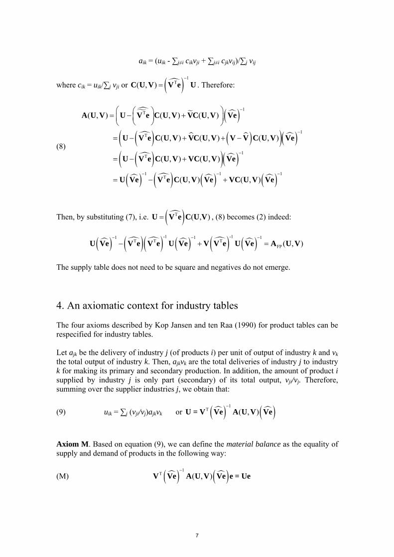
Then, by substituting (7), i.e. ( ) ( , )Τ=U V e C U V , (8) becomes (2) indeed:

( ) ( )( ) ( ) ( ) ( )1 11 1 1

FP ( , )− − −

Τ Τ Τ− + =- -

U Ve V e V e U Ve V V e U Ve A U V

The supply table does not need to be square and negatives do not emerge. 4. An axiomatic context for industry tables The four axioms described by Kop Jansen and ten Raa (1990) for product tables can be respecified for industry tables. Let ajk be the delivery of industry j (of products i) per unit of output of industry k and vk the total output of industry k. Then, ajkvk are the total deliveries of industry j to industry k for making its primary and secondary production. In addition, the amount of product i supplied by industry j is only part (secondary) of its total output, vji/vj. Therefore, summing over the supplier industries j, we obtain that:

(9) uik = ∑j (vji/vj)ajkvk or ( ) ( )1T ( , )

−U = V Ve A U V Ve

Axiom M. Based on equation (9), we can define the material balance as the equality of supply and demand of products in the following way:

(M) ( ) ( )1T ( , )

−V Ve A U V Ve e = Ue

7

Axiom F. Dual to the material balance is the financial balance, where supply and demand for all industries must be coincident. Notice that axiom M is defined by the equivalence of the row sums of both sides of equation (9) while the axiom F will be defined by the column sums instead. The financial balance equates revenues and costs for all sectors and reads:

(F) ( ) ( )1T T T( , )

−

e V Ve A U V Ve = e U

Axiom P. In the spirit of Kop Jansen and ten Raa (1990), price invariance avoids the possibility that a change in the base year prices could affect industry coefficients. Equation (9) becomes for industry j:

( , )= ji

j jik i ik ikjk

ji k ji ki ji ki

vv vu uav v v v v v

• u

•

= =∑

∑e

U Ve

where is the row vector of product outputs of industry j and jv •e kv •e the same but for industry k. Revaluating intermediate uses by piuik and commodity outputs by pivji, we can write:

ˆ ˆ( , ) =

= (

i jiji i ik ik

jki ji i ki ji k

i

j j jik k kjk

j ji k k j k

p v vp u uap v p v v v

v v vu v vav v v v v v

•

•

• • •• •

• • • •

= =

=

∑∑

ppU Vp

p

e p pe eU Ve p e e

, )•p

Now, since is the j-th element of the main diagonal of jv •e ( )Ve and likewise for

industry k, can also be considered to be the j-th element of the main diagonal

of . The same applies for industry k,

jv •p

(Vp) kv •p . Hence, in matrix terms, the price

invariance is given by:

(P) ( )( ) ( )( )1 1ˆ ˆ( , ) = ( , )

− −A pU Vp Vp Ve A U V Ve Vp for all p > 0

Axiom S. The scale invariance considers multiplication of inputs and outputs of industries by factors. So, we multiply all product requirements and outputs of industry 1 by a common scale factor, say s1, and likewise for other industries. From equation (9):

( , )= ji

i ikjk

ji kii

vua

v v

∑∑

U V

8

and by re-scaling, we obtain:

ˆ ˆ( , )= = = ( , )ji j j ji

i ik k i k ikjk jk

ji j ki k j ji k kii i

v s s vu s s ua a

v s v s s v s v

∑ ∑∑ ∑

Us sV U V

Axiom S postulates that industry coefficients should not change when input requirements and product outputs vary proportionally. So, for all industries, it must be that: (S) ˆ ˆ( , ) ( , )=A Us sV A U V for all s > 0

The axiom is not a constant returns to scale assumption, but merely postulates that if industry coefficients are constant for each product, then industry coefficients must be fixed (Kop Jansen and ten Raa, 1990). 5. Performance Table 1 summarizes the results of the performance of models (1) and (2).The fixed industry sales structure model (1) fulfils all the four axioms while the fixed product sales structure model (2) only fulfils the financial balance. This is not surprising since the financial balance accounts for the equality between supply and demand of industry outputs and the industry by industry input-output tables are balanced. Proofs of the latter are relegated to the Appendix.

TABLE 1 PERFORMANCE OF IO CONSTRUCTS FOR INDUSTRY TABLES

Material balance Model Financial

balance Price

invariance Scale

invariance Fixed industry sales structure √ √ √ √

Fixed product sales structure √

Theorem 3. The input-output industry coefficients derived from the fixed industry sales structure model are industrial and financially balanced; and price and scale invariant. Proof. From (1), we obtain for Axiom M that:

( ) ( ) ( ) ( ) ( ) ( )1 1T T T

FI

T T

( , )− −

−

−

V Ve A U V Ve e = V Ve Ve V U Ve Ve e =

= V V Ue = Ue

1−

For the financial balance,

9

( ) ( ) ( ) ( ) ( ) ( )1 1T T T T T

FI

T T T T

( , )− −

−

−

e V Ve A U V Ve = e V Ve Ve V U Ve Ve =

= e V V U = e U

1−

For the price invariance axiom,

( )( )( ) ( )( ) ( ) ( )( ) ( ) ( )( ) ( ) ( ) ( )( )( )( ) ( )( )

1 1T T 1FI

1 1 1T T

1 1

FI

ˆ ˆ ˆ ˆ ˆ ˆ ˆ ˆ ˆ ˆ( , )

( , )

− −

− − −

− −

=

= =

=

- - -

- -

A pU Vp = Vp e Vp pU Vp e Vpe V p pU Vpe

Vp V U Vp Vp Ve Ve V U Ve Ve Vp

Vp Ve A U V Ve Vp

1−

And for axiom S,

( )( )( ) ( )( ) ( ) ( )( ) ( )

1 1T 1 T 1FI

1T

FI

ˆ ˆ ˆ ˆ ˆ ˆ ˆˆ ˆˆ( , )

( , )

− −

−

=

=

- - - -

-

A Us sV = sV e sV Us sV e Ve ss V Uss Ve

Ve V U Ve = A U V

since . ( ) ( ) ( )ˆ ˆΤ Τ=sV e e V s = Ve s

We may conclude that the fixed industry sales structure model is axiomatically

the best one to construct industry coefficients. Furthermore, since the fixed industry sales structure assumption depends on the inverse of the supply matrix, it also must be square and may cause negatives as well as the product technology model for product tables. Conversely, the fixed product sales structure model has the advantage of coming out without negatives.

6. Characterization Following the first work providing a characterization result concerning the construction of input-output coefficients for product tables (Kop Jansen and ten Raa, 1990), this paper provides the other side of the coin, i.e. two characterization theorems for the construction of industry tables. This aims to an almost definite debate settlement than the previous literature which it was mainly devoted to the comparison of alternative methods and to product tables. This section shows the main results. They determine the fixed industry sales structure model as the single method that fulfils the desirable properties listed in the fourth section. As a matter of fact, if we accept one balance and one invariance axiom, then we must impose the fixed industry sales structure model. Theorem 4. (real sphere) The material balance and scale invariance axioms characterize the fixed industry sales structure model.

10

Proof. The fixed industry sales structure model implies that the material balance and scale invariance axioms hold by Theorem 3. Conversely, let us assume that the material balance and scale invariance are met. By axiom M,

( ) ( )1T ( , )

−

V Ve A U V Ve e = Ue

for all A(U,V). Replace . Then ˆ ˆ( , )A Us sV

( ) ( )( ) ( )( )1Tˆ ˆ ˆ ˆ ˆ( , )−

sV sV e A Us sV sV e e = Useˆ .

By axiom S and since and se , ( )( ) ( )ˆ =sV e Ve s = s

( )( ) ( )1

Tˆ ˆ ( , )−

V s Ve s A U V Ve s = Us

being:

( ) ( ) ( ) ( )1 1

T 1 Tˆˆ ( , ) ( , )− −

−V ss Ve A U V Ve s = V Ve A U V Ve s = Us .

Since this holds for all positive s and thus for a basis, the matrices acting on them must be equal:

( ) ( )1

T ( , )−

V Ve A U V Ve = U

Therefore,

( ) ( )1

T( , )−

−A U V = Ve V U Ve . Theorem 5. (nominal sphere) The financial balance and price invariance axioms characterize the fixed industry sales structure model. Proof. Necessity has already been proved in Theorem 3. For the sufficiency proof, let us assume that the financial balance and price invariance axioms hold. By axiom F,

( ) ( )1T T T( , )

−

e V Ve A U V Ve = e U

for all A(U,V). Substitute . Then: ˆ ˆ( ,A pU Vp)

( ) ( )( ) ( )( )1TT Tˆ ˆ ˆ ˆ ˆ ˆ( , )−

e Vp Vp e A pU Vp Vp e = e pU

11

for which the LHS, since , is: T T Tˆe pV = p VT

( ) ( ) ( ) ( )( ) ( )( ) ( )( ) ( )( ) ( )

1 1T T T T

1 1 1T T

1T T

ˆ ˆ ˆ ˆ ˆ ˆ( , ) ( , )

( , )

( , )

− −

− − −

−

= =

=

=

p V Vpe A pU Vp Vpe p V Vp A pU Vp Vp

p V Vp Vp Ve A U V Ve Vp Vp

p V Ve A U V Ve

and then, since : T Tˆe pU = p U

( ) ( )1T T T( , )

−

=p V Ve A U V Ve p U .

Since this is true for all p > 0, we may proceed to conclude that:

( ) ( )1T ( , )

−

=V Ve A U V Ve U

and hence (1). 7. Conclusions Product tables and industry tables coexist and each type can be constructed in accordance with a product or an industry based model. For product tables, it is well accepted that the product (technology) model is superior to the industry (technology) model, on the basis of the axiomatic analysis of Kop Jansen and ten Raa (1990). This paper brings in two characterization theorems for industry tables and argues that the fixed industry sales structure model emerges as the best one to construct industry tables in comparison with the fixed product sales structure model. At least in principle, this argument provides a justification for the current statistical practices in Canada, Denmark, Finland, the Netherlands and Norway, although they most frequently use the fixed product sales structure assumption (also free from negatives) instead. References Eurostat (2008) Eurostat Manual of Supply, Use and Input-Output Tables (Luxembourg:

Eurostat). Kop Jansen, P. and ten Raa, T. (1990) “The Choice of Model in the Construction of Input-

Output Coefficients Matrices”, International Economic Review, 31, pp. 213-227. Rueda-Cantuche, J.M. (2008) “Análisis Input-output Estocástico de la Economía Andaluza”.

Ph. D. Dissertation, Institute of Statistics of Andalusia, (in press) [available in English upon request to the author].

ten Raa, T. (2004) Structural Economics (London: Routledge).

12

ten Raa, T. (2005) The Economics of Input-Output Analysis (Cambridge: Cambridge University Press).

ten Raa, T. and Rueda-Cantuche, J.M. (2003) “The Construction of Input-Output Coefficients Matrices in an Axiomatic Context: Some Further Considerations”, Economic Systems Research, 15, 439-455.

ten Raa, T. and Rueda-Cantuche, J.M. (2007) “A generalized expression for the commodity and the industry technology models in input-output analysis”, Economic Systems Research, 19, 99-104.

Thage, B. and ten Raa, T. (2007) “Streamlining the SNA 1993 chapter on Supply and Use Tables and Input-Output”, paper presented at the 29th General Conference of the International Association for Research in Income and Wealth, Joensuu, Finland.

United Nations (1993) Revised System of National Accounts, Studies in Methods, Series F, no. 2, rev.4 (New York: United Nations).

Yamano, N. and N. Ahmad (2006), “The OECD Input-Output Database: 2006 Edition”, OECD Science, Technology and Industry Working Papers, 2006/8, OECD Publishing doi:10.1787/308077407044.

Appendix This Appendix details the performance of the fixed product sales structure model for industry tables. It fulfils only the financial balance axiom. By using the same fictitious use and supply matrices (originally make matrix) as in Kop Jansen and ten Raa (1990), we will present counterexamples that violate some of the balance axioms. Axiom F Since equation (2) provides the formulation of the fixed product sales structure model and (F) the financial balance, by substitution in the LHS of (F):

( ) ( ) ( ) ( ) ( )1 11 1T T T T T

− −− −

=e V Ve V V e U Ve Ve e V V e U .

Therefore, since and (T T Te V = e Ve) ( )T T Te V = e V e , then:

( )( ) 1T T T T

−

=e V e V e U e U .

Axiom M Let us define the following use and make tables:

1/ 2 0 1 1 2; ;

1 1/ 2 0 1 1⎛ ⎞ ⎛ ⎞

= = =⎜ ⎟ ⎜ ⎟⎝ ⎠ ⎝ ⎠

U V p ⎛ ⎞= ⎜ ⎟⎝ ⎠

s

A straightforward computation shows that:

13

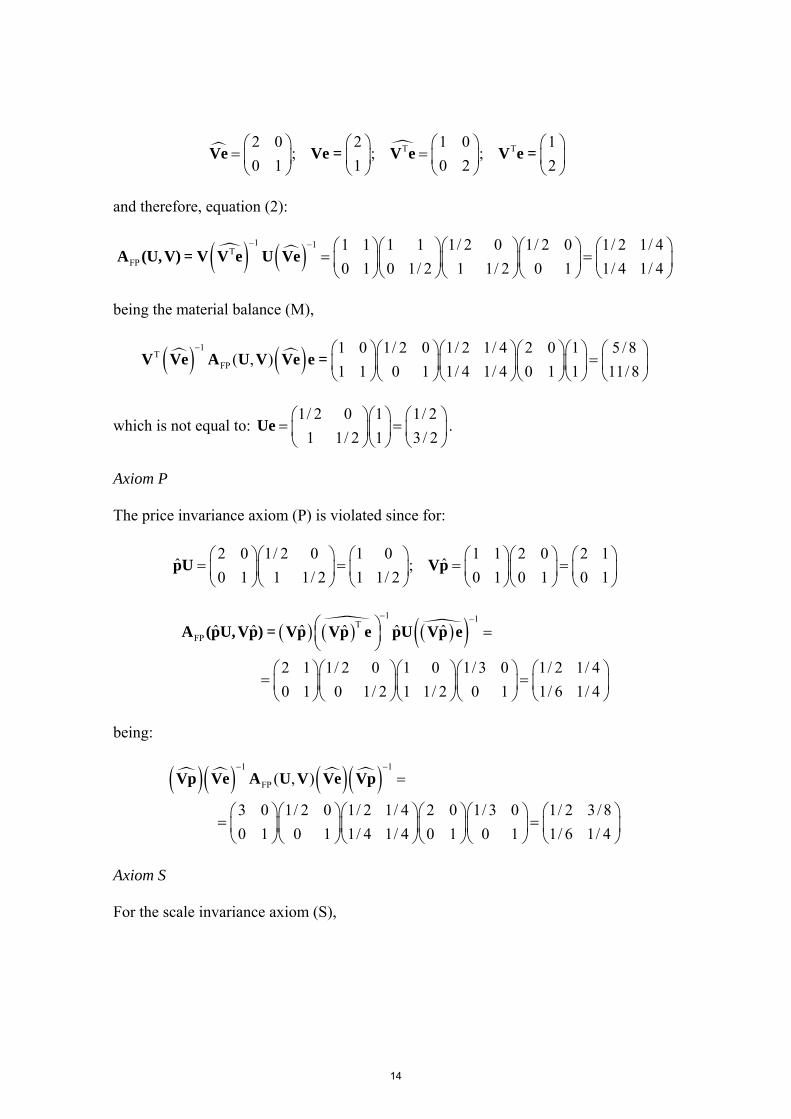
2 0 2 1 0 1

; ; ;0 1 1 0 2 2

Τ Τ⎛ ⎞ ⎛ ⎞ ⎛ ⎞ ⎛ ⎞= =⎜ ⎟ ⎜ ⎟ ⎜ ⎟ ⎜ ⎟⎝ ⎠ ⎝ ⎠ ⎝ ⎠ ⎝ ⎠

Ve Ve = V e V e =

and therefore, equation (2):

( ) ( )1 1

FP

1 1 1 1 1/ 2 0 1/ 2 0 1/ 2 1/ 40 1 0 1/ 2 1 1/ 2 0 1 1/ 4 1/ 4

− −Τ ⎛ ⎞⎛ ⎞⎛ ⎞⎛ ⎞ ⎛

= =⎜ ⎟⎜ ⎟⎜ ⎟⎜ ⎟ ⎜⎝ ⎠⎝ ⎠⎝ ⎠⎝ ⎠ ⎝

A (U,V) = V V e U Ve ⎞⎟⎠

⎞⎟⎠

⎞⎟⎠

⎞= ⎟

⎠

being the material balance (M),

( ) ( )1T

FP

1 0 1/ 2 0 1/ 2 1/ 4 2 0 1 5 / 8( , )

1 1 0 1 1/ 4 1/ 4 0 1 1 11/ 8

− ⎛ ⎞⎛ ⎞⎛ ⎞⎛ ⎞⎛ ⎞ ⎛=⎜ ⎟⎜ ⎟⎜ ⎟⎜ ⎟⎜ ⎟ ⎜

⎝ ⎠⎝ ⎠⎝ ⎠⎝ ⎠⎝ ⎠ ⎝V Ve A U V Ve e =

which is not equal to: . 1/ 2 0 1 1/ 2

1 1/ 2 1 3/ 2⎛ ⎞⎛ ⎞ ⎛

= =⎜ ⎟⎜ ⎟ ⎜⎝ ⎠⎝ ⎠ ⎝

Ue

Axiom P The price invariance axiom (P) is violated since for:

2 0 1/ 2 0 1 0 1 1 2 0 2 1ˆ ˆ;

0 1 1 1/ 2 1 1/ 2 0 1 0 1 0 1⎛ ⎞⎛ ⎞ ⎛ ⎞ ⎛ ⎞⎛ ⎞ ⎛

= = =⎜ ⎟⎜ ⎟ ⎜ ⎟ ⎜ ⎟⎜ ⎟ ⎜⎝ ⎠⎝ ⎠ ⎝ ⎠ ⎝ ⎠⎝ ⎠ ⎝

pU Vp

( ) ( ) ( )( )1 1

FP ˆ ˆ ˆ ˆ ˆ ˆ

2 1 1/ 2 0 1 0 1/ 3 0 1/ 2 1/ 40 1 0 1/ 2 1 1/ 2 0 1 1/ 6 1/ 4

− −Τ⎛ ⎞ =⎜ ⎟⎝ ⎠

⎛ ⎞⎛ ⎞⎛ ⎞⎛ ⎞ ⎛ ⎞= =⎜ ⎟⎜ ⎟⎜ ⎟⎜ ⎟ ⎜ ⎟⎝ ⎠⎝ ⎠⎝ ⎠⎝ ⎠ ⎝ ⎠

A (pU,Vp) = Vp Vp e pU Vp e

being:

( )( ) ( )( )1 1

FP ( , )

3 0 1/ 2 0 1/ 2 1/ 4 2 0 1/ 3 0 1/ 2 3/ 80 1 0 1 1/ 4 1/ 4 0 1 0 1 1/ 6 1/ 4

− −

=

⎛ ⎞⎛ ⎞⎛ ⎞⎛ ⎞⎛ ⎞ ⎛= =⎜ ⎟⎜ ⎟⎜ ⎟⎜ ⎟⎜ ⎟ ⎜⎝ ⎠⎝ ⎠⎝ ⎠⎝ ⎠⎝ ⎠ ⎝

Vp Ve A U V Ve Vp

⎞⎟⎠

Axiom S For the scale invariance axiom (S),

14

( ) ( ) ( )( )1 1

FP ˆ ˆ ˆ ˆ ˆ ˆ

2 2 1/ 2 0 1 0 1/ 4 0 7 /12 1/ 30 1 0 1/ 3 2 1/ 2 0 1 1/ 6 1/ 6

− −Τ⎛ ⎞ =⎜ ⎟⎝ ⎠

⎛ ⎞⎛ ⎞⎛ ⎞⎛ ⎞ ⎛= =⎜ ⎟⎜ ⎟⎜ ⎟⎜ ⎟ ⎜⎝ ⎠⎝ ⎠⎝ ⎠⎝ ⎠ ⎝

A (Us,sV) = sV sV e Us sV e

⎞⎟⎠

and

FP

1/ 2 1/ 41/ 4 1/ 4⎛ ⎞⎜ ⎟⎝ ⎠

A (U,V) = ,

are different and hence, (S) does not hold.

15