Embed Size (px)
Citation preview
18‐893
“ComputerizingIndustriesandRoutinizingJobs:ExplainingTrendsinAggregateProductivity”
SangminAum,SangYoon(Tim)LeeandYongseokShin
Februray2018

Computerizing Industries and Routinizing Jobs:Explaining Trends in Aggregate Productivity∗
Sangmin Aum† Sang Yoon (Tim) Lee‡ Yongseok Shin§
February 21, 2018
Abstract
Aggregate productivity growth in the U.S. has slowed down since the 2000s. We
quantify the importance of differential productivity growth across occupations and
across industries, and the rise of computers since the 1980s, for the productivity slow-
down. Complementarity across occupations and industries in production shrinks the
relative size of those with high productivity growth, reducing their contributions to-
ward aggregate productivity growth, resulting in its slowdown. We find that such a
force, especially the shrinkage of occupations with above-average productivity growth
through “routinization,” was present since the 1980s. Through the end of the 1990s,
this force was countervailed by the extraordinarily high productivity growth in the
computer industry, of which output became an increasingly more important input in
all industries (“computerization”). It was only when the computer industry’s produc-
tivity growth slowed down in the 2000s that the negative effect of routinization on
aggregate productivity became apparent. We also show that the decline in the labor
income share can be attributed to computerization, which substitutes labor across all
industries.
∗This paper was prepared for the Carnegie Rochester NYU Conference on “the Consequences of Trans-formative Technical Progress for the Macroeconomy.” We thank our discussant, Matthias Kehrig, for excep-tionally detailed and constructive suggestions, and other conference participants for many useful comments.We also benefited from extended conversations about this paper with Christian Siegel, Henry Siu, and SevinYeltekin. The usual disclaimer applies.†Washington University in St. Louis: [email protected].‡Toulouse School of Economics and CEPR: [email protected].§Washington University in St. Louis, Federal Reserve Bank of St. Louis and NBER: [email protected].
1

1 Introduction
Amid the sluggish recovery following the Great Recession, much attention has been
given to the slowdown in productivity growth in the United States economy (sometimes
referred to as “secular stagnation”). We dissect this trend in aggregate productivity
by developing a model in which technological progress is both sector- and occupation-
specific,1 to better understand which sectors and occupations contribute most to trends
in aggregate productivity.2 In particular, we pay special attention to the computer
sector (hardware and software), which enjoyed an impressive rise in productivity even
as the rest of the economy lagged behind. Computers have become an important
factor of production for all other sectors, especially since the 1990s (which we call
“computerization”), so we separate them from other machinery equipment as a distinct
type of capital. Using the model, we quantify the importance of the computer sector
and compare it against “routinization” (i.e., faster technological progress specific to
occupations that involve routine or repetitive tasks) in explaining trends in aggregate
productivity.
We find that a downward trend in aggregate productivity growth was already
present since the 1970s, but that this was more than compensated for by the ex-
traordinary productivity growth of the computer sector in the 1980s and 1990s. It was
only when the computer sector’s productivity growth came down to normal levels in
the 2000s that the deceleration in aggregate productivity became abruptly apparent.
This generated the illusion that the aggregate productivity slowdown has its roots in
the 2000s, even though the slowdown had already been underway in the preceding
decades.
In our analysis, the driving force of the aggregate productivity slowdown is comple-
mentarity across occupations and across industries in production: Those occupations
and industries with above-average productivity growth shrink in terms of value-added
and employment shares, and their contributions toward aggregate productivity growth
becomes smaller even when their productivity continues to grow fast. This is related
to “Baumol’s disease,” i.e., that aggregate productivity growth can slow down because
sectors with high productivity growth may decline in importance (e.g., manufacturing).
However, our results show that it is the shrinkage of occupations with fast occupation-
1Throughout the text, we will use “sector” and “industry” interchangeably, as well as “occupations” and“jobs.”
2Our model will admit an aggregate productivity that is distinct from conventional measures of totalfactor productivity (TFP), which assumes a homogeneous of degree one (HD1) production function in thetwo factors of capital and labor. When distinction is necessary, we will refer to our version with three factors(capital, labor and computers) simply as “productivity,” and the two-factor residual as “TFP.”
2

specific productivity growth, not sectors, that accounts for most of the downward trend
in aggregate productivity growth.
Another novel element of our analysis is the computer sector. When sectors are
complementary to one another, the extraordinarily high productivity growth of the
computer sector should reduce its relative importance, and hence its contribution to
aggregate productivity growth over time (Baumol’s disease). However, because we
model the computer sector’s output as a distinct type of capital used in the production
of all sectors (including itself), its productivity growth and the accompanying fall in
its price boost the demand for computers from all sectors. Consequently, the computer
sectors’s contribution to aggregate productivity remained important for a prolonged
period of time, more than offsetting the negative effect of routinization on aggregate
productivity growth for over two decades. We also show that computerization accounts
for most of the decline in the labor income share since the 1980s.
In our model, individuals inelastically supply labor to differentiated jobs. Each
sector uses all these jobs, but with different intensities. Sectors are complementary
across one another for the production of the final good. Within each sector, jobs are
also complementary to one another, and labor is combined with capital for sectoral
production. Most important, we divide capital into computer capital (including soft-
ware) and the rest (i.e., all capital not produced from the computer sector), and assume
that the substitutability between labor and computer capital may differ across sectors.
We model computer and software as capital used by all other sectors rather than an
intermediate input, because the computer share of all investment is substantially larger
than its share of all intermediates (14 vs. 2 percent, averaged between 1980 and 2010).
It should be noted that computerization and routinization are empirically distinct
phenomena. Computer and software usage increased the most for high-skill or cog-
nitive occupations, not middle-skill or routine occupations (Aum, 2017), justifying
our choice to model productivity growth in both dimensions (sector- and occupation-
specific). We then estimate the degree of complementarity across sectors, and calibrate
the growth rates of the sector- and occupation-specific productivities, substitutabil-
ity/complementarity across jobs, and substitutability between computer capital and
labor, using detailed data on employment shares and computer capital by industry
and by occupation. Our estimation and calibration verify that as long as productiv-
ity growth rates are positive, (i) sectors are complementary to one another for final
good production;3 (ii) jobs are complementary to one another within sectors; and most
important, (iii) computer capital is in fact substitutable with labor in all sectors.
3Or consumption, which we do not model.
3
Given the structure of our model and estimated/calibrated parameters, we find
that when sector- and occupation-specific productivities grow at constant but different
rates, aggregate productivity growth declines over time due to the two types of com-
plementarity (across jobs within sectors, and across sectors in final good production).
Jobs and sectors with highest productivity growth shrink in terms of employment and
value-added. Then low-growth jobs and sectors gain more weight when computing ag-
gregate productivity growth, resulting in its slowdown. As productivity growth slows
down, output growth slows down even more.
The mechanics of our model is consistent with our empirical findings: Since the
1980s, sectors that rely heavily on routine jobs experienced the highest growth in their
TFP’s, as measured by conventional growth accounting.4 These occupations, and the
sectors that rely relatively more on them, also saw their employment shares fall.
Next, we find that the fall in aggregate productivity growth in the longer run is
more due to the differential growth across occupations (i.e., routinization) rather than
the differential growth across sectors. In fact, if all occupation-specific productivities
had grown at a common rate from 1980, holding all else equal, aggregate produc-
tivity growth rates would have stayed nearly constant through 2010. This contrasts
with Baumol’s disease, which emphasizes the differential sector-specific productivity
growths, especially the slow productivity growth of the service sector.
The natural question is then why the downward trend in aggregate productivity
growth did not manifest itself until the 2000s. In our model, the slowdown in aggregate
productivity growth can be temporarily arrested and even reversed if certain sectors or
jobs experience faster-than-usual technological progress. We find that this is exactly
what happened during the 1990s, when the computer sector recorded impressive pro-
ductivity growth. Without the technological progress specific to the computer industry,
aggregate productivity growth during the 1990s would have been 0.5 percent per year,
instead of 0.8 percent. It is only after the subsequent slowdown in the computer sector’s
productivity growth in the 2000s that the longer-run downward trend in aggregate pro-
ductivity growth became apparent. Our analysis confirms that if productivity growth
in the computer sector had been completely absent, aggregate productivity growth
would have declined monotonically since 1980. In fact, although our focus is on the
slowdown toward the end of the sample period in Figure 1, a slowdown is also apparent
in the 1970s to early 1980s.
4That is, assuming an HD1 production function with two factors, capital and labor. By “measured,”we mean productivity or TFP obtained directly from the data by growth accounting, as opposed to beingcomputed from our model.
4

0.2
.4.6
.8
1950 1960 1970 1980 1990 2000 2010
Period d logTFP
1950- 1.201960- 1.351970- 0.591980- 1.141990- 1.462000- 1.032010- 0.38
Fig. 1: Log TFP, AggregateSource: National Income and Product Accounts (NIPA) from the Bureau of Economic Analysis (BEA).TFP is measured as the Solow residual assuming a homogeneous of degree one production function with twofactors, capital and labor.
In the data, sectors with higher measured TFP growth saw their employment shares
decline, except for the computer sector. The same happens in our model because all
sectors use computer capital in production. Then, as the computer sector’s productivity
growth reduces the price of computer capital, all sectors use more computers, which
contributes to output growth in addition to the computer sector’s direct contribution
to aggregate productivity growth.5 Indeed, if there had been no productivity growth
in the computer sector and hence no computerization, output per worker growth would
have been 1.5 percent per year during the 1990s, rather than the 3.5 percent observed
in the data. In other words, the sluggish growth of aggregate productivity and output
in the 2000s was not abnormal. It was the faster-than-trend growth during the 1990s
driven by the outburst of the computer sector’s productivity that was extraordinary.
Treating computer capital as a separate production factor as we do also has impli-
cations for the measurement of aggregate productivity. We find that conventional TFP
accounting with only two factor inputs, with all types of capital being summed up into
a single category, overstates aggregate productivity growth by 0.4 percentage points per
5As discussed earlier, this model element is also important for understanding why the direct contributionof the computer sector to aggregate productivity growth did not dwindle in importance despite the comple-mentarity across sectors. The computer sector’s production share has been stable over time: 3.1 percent inthe 1980s, 3.4 percent in the 1990s, 3.9 percent in the 2000s, and 3.4 percent in the 2010s.
5

year when averaged between 1980 and 2010. That is, ignoring different types of capital,
which differ in their rental and depreciation rates, can bias productivity measurements
upward.
Lastly, we relate computerization to the decline in the labor income share. In our
model, the labor share decline is caused by the substitutability between labor and
computer capital, as the computer sector becomes more productive. We find that
computerization during the 1990s accounts for most of the decline in the labor share
between 1980 and 2010 (4 out of 5 percentage points), even the model does not target
the labor share at all. This implies that computer capital alone is more important than
all other machinery and equipment in explaining the decline in the labor share.
Related literature In our model, employment shifts across sectors—or “structural
change”—occur due to differential sector- and occupation-specific productivity growth
as in Lee and Shin (2017). Most studies in the structural change literature that consider
sector-specific productivity growth, e.g., Ngai and Pissarides (2007), have paid little
attention to its implications for changes in aggregate productivity. In fact, most were
interested in obtaining balanced growth. However, since as far back as Baumol (1967),
it was well known that complementarity between industries can lead to an increase
in the employment share of the low productivity growth sector, consequently leading
to a slowdown in aggregate productivity. A recent study by Duernecker, Herrendorf,
and Valentinyi (2017) is a notable exception. They explicitly consider Baumol’s dis-
ease in a multi-sector model, and evaluate whether structural change is quantitative
important for explaining the aggregate productivity slowdown. In our analysis, we
model differential progress across occupation-specific technologies in addition to het-
erogeneous sector-specific productivity growth, and find that it was the dispersion of
occupation-specific productivities that was more important for the aggregate produc-
tivity slowdown in the United States.6
Our work also relates to studies on the importance of information technology (IT)
in explaining the evolution of productivity (e.g., Byrne, Fernald, and Reinsdorf, 2016;
Syverson, 2017). In particular, Acemoglu, Autor, Dorn, Hanson, and Price (2014)
investigate the relationship between productivity growth and IT capital intensity by
industry, and conclude that IT usage has little impact on productivity. While we
emphasize the role of computerization, our analysis is consistent with theirs. Com-
puterization is important for shaping aggregate productivity growth in our analysis,
6Aum, Lee, and Shin (2017) document occupation-specific and sector-specific shocks at a higherfrequency—during and after the Great Recession.
6

but there is no direct effect of computerization on the productivity of other indus-
tries. Instead, computerization affects industry level output and value-added through
an increase in the use of computer capital.
In many empirical analyses related to routinization, the price of information and
communication technology (ICT) capital is often used as a proxy for routine-biased
technological change (e.g., Goos, Manning, and Salomons, 2014; Cortes, Jaimovich,
and Siu, 2017). However, when we break down computer usage by occupation, we find
that computerization and routinization are two distinct phenomena, with different im-
plications for the macroeconomy. Related, Aum (2017) analyzes increasing investment
in software in a model that also features routinization. While Aum (2017) focuses on
its impact on changes in occupational employment, we focus on its implications for
aggregate productivity.
Finally, Karabarbounis and Neiman (2014) suggest that the decline in the labor
income share could be due to a decline in the price of capital. Since the decline in
the price of capital is mostly driven by the price of computer-related equipment, and
it mirrors the productivity increase in the computer industry, our analysis concurs
with their explanation of the declining labor share. Furthermore, our results show
that a specific component of capital—computer hardware and software—can be more
important than all other types of capital. This is in line with Koh, Santaeullia-Llopis,
and Zheng (2016), who emphasize the importance of intellectual property products
capital (including software) for the decline of the labor share.
2 Empirical Evidence
We begin by establishing that routinization and computerization are two distinct phe-
nomena. For the empirical analysis, occupational data is from the decennial censuses
and industrial data from the BEA industry accounts. We consider industries at the
2-digit level, resulting in 60 industries. In particular, we label industry 334 (computers
and electronic products) the “hardware” industry and 511 (publishing industries in-
cluding software) the “software” industry. The combination of both is the “computer
sector.”
In Figure 2(a), the horizontal axis is occupational employment shares (percentile),
in ascending order of each occupation’s 1980 average wage.7 The figure shows that the
routine-task intensity (RTI) of occupations (Autor and Dorn, 2013) is high for middle-
wage occupations, as is well known in the routinization/polarization literature, but
7The ordering of occupational mean wages barely changes from 1980 to 2010.
7

.1.2
.3.4
.5.6
−2
−1
01
2
0 20 40 60 80 100
Hardware (L) Software (L)Routine task share (R)
(a) Routinization and computerization
01
23
45
1980 1990 2000 2010
Hardware (334) Software (511)Computer (334+511) All industries
(b) log-TFP of computer industry
Fig. 2: PC use by occupation and PC industry TFPSource: (a) IPUMS Census, BEA NIPA and O*NET. (b) BEA Industry Accounts. The computer industryincludes industries 334 and 511 (for hardware and software, respectively). See footnote 8 and text for thedata and accounting behind the graphs.
that high-wage occupations tend to use computers more.8 So at the occupational level,
an increase in the use of computers (i.e., computerization) should be distinguished
from routinization, which is typically understood as faster productivity growth among
middle-wage or routine-intense tasks.
Computerization in our model is a consequence of the fast productivity growth
of the computer industry. We first employ conventional accounting to measure each
industry’s TFP growth: the growth rate of real value-added net of the growth of capital
and labor inputs, weighted by the income share of each factor. Specifically, industry
i’s measured TFP growth between time s and t is
logTFPitTFPis
= logYitYis− αis + αit
2· log
LitLis− 2− αis − αit
2· log
Kit
Kis,
where Y is real value-added, L is employment, K is the net real stock of non-residential
fixed capital, and α is the labor share (compensation of employees divided by value-
8Computer usage is approximated from 2010 NIPA Tables 5.5.5 (Private Fixed Investment in Equipmentby Type), 5.6.5 (Private Fixed Investment in Intellectural Properties by Type), and the O*NET Tools andTechnology database as follows. In NIPA Table 5.5.5, we assume that “computers and peripheral equipment”are produced by industry 334, and in Table 5.6.5, that “software” are produced by industry 511. O*NETlists all the tools and technology that are used for each occupation. O*NET occupation codes can be easilymapped to the census, and tools and technology are coded using the UNSPSC commodity system. Weassume that 4321xxxx corresponds to “hardware,” which includes all computers and peripheral equipment,and that 4323xxxx corresponds to “software.” Then we count the number of distinct commodities neededin each occupation, multiply it by the employment share of that occupation, and assume that hardware andsoftware investment is allocated across occupations proportionately to this number. Finally, we standardizethis measure of computer investment by occupation to have a mean of zero and standard deviation of 1.While this may be a crude measure for computer usage, it is highly correlated with data from the CPS,which reports computer use intensity by occupation. See Appendix A of Aum (2017) for more details.
8

11.
52
2.5
3
1970 1980 1990 2000 2010
Hardware Hardware + Software
(a) Computer share of intermediates (%)
05
1015
20
1970 1980 1990 2000 2010
Hardware Hardware + Software
(b) Computer share of non-residential investment (%)
Fig. 3: Computer use in production over timeSource: BEA Input-Output Tables and Fixed Asset Tables (FAT). In panel (a), hardware and software areindustries 334 and 511. In panel (b), hardware and software are investments into “computers and peripheralequipment” and “software” in the FAT.
added).9
Figure 2(b) depicts the log-TFP of computer-related industries (BEA industry code
334 for hardware and 511 for software) and the average of the log-TFP of all industries
excluding agriculture and government (weighted according to the Tornqvist index).
The TFP of hardware shows an average annual growth rate of 16 percent, far higher
than the average across all industries. Software also features higher TFP growth
compared to the average. The TFP of the “computer industry”—the value- added
weighted average of hardware and software—shows that the hardware industry mostly
determines the TFP of the computer industry. Note that the exceptionally fast growth
of the computer industry’s TFP slowed down since around the early 2000s.
Reflecting the fast growth of the computer industry’s measured TFP, the use of
computer and software also rose substantially until the late 1990s. Figure 3(a) shows
the computer and software share of total intermediates over time. Figure 3(b) plots the
share of computers and software in total non-residential investment. In both figures,
it is clear that there was a steep rise in the importance of computers in the 1980s to
1990s, which stagnated starting in the 2000s.10
We now turn to disaggregated evidence at the industry level, which will support
our hypotheses of heterogeneous growth rates and complementarity across jobs and
industries. Because job or occupation-level productivity is not directly measurable, we
9Later when we separately consider computer capital, TFP computed here would be a misspecification.10The data behind Figures 3(a) and (b) come from BEA’s Input-Output Tables and Fixed Assets Tables,
respectively.
9

Hardware
Software
−10
00
100
200
300
400
TF
P g
row
th (
1980
−20
10)
0 20 40 60 80Routine job share (1980)
(a) Routine occupation share and TFP growth
Hardware
Software
−10
00
100
200
300
400
TF
P g
row
th (
1980
−20
10)
−2 −1 0 1 2Employment growth (1980−2010)
(b) TFP and employment growth across industries
Fig. 4: Routinization and industry TFP and employmentSource: IPUMS Census and BEA Industry Accounts. Hardware and Software are industries 334 and 511,respectively. In panel (a), routine jobs are defined as occupations above the 66 percentile in terms of theRTI index (Autor and Dorn, 2013). In panel (b), FTPT is full-time plus part-time workers.
first establish two new empirical patterns, utilizing the fact that industries differ in the
composition of their workers’ occupations. Figure 4(a) shows that the routine job share
of an industry is positively correlated with its measured TFP growth (log difference)
between 1980 and 2010 (consistent with routinization), where routine jobs are defined
as occupations that are above the 66 percentile in terms of the RTI index following
Autor and Dorn (2013). Figure 4(b) shows that TFP growth and employment growth
are negatively correlated across industries, consistent with complementarity across jobs
and/or industries.11
However, note that the computer industry is a conspicuous outlier. In Figure 4(a),
despite having a routine job share around the median, not only is the computer indus-
try’s TFP growth 10 times larger than other industries at similar levels of routineness,
it is in fact 2 to 4 times larger than the next two industries with the highest levels of
TFP growth overall. Despite this, as shown in Figure 4(b), its employment barely fell.
With complementarity across industries, a high productivity growth sector should lose
value-added and employment shares. A possible explanation is that other industries
depend heavily on the computer industry, so that even as its productivity grows the
size of this sector would not shrink as long as other industries rely on it more. If so,
those industries with faster growth in computer capital should grow faster than those
that use computers less intensively in terms of output : since computer capital is a fac-
11Employment in this figure is full-time plus part-time workers (FTPT). Full-time equivalent (FTE)employment shows similar patterns, but is only available by industry from 1997 onward. For this period,there are level differences between the two measures, but dynamic patterns are similar for both.
10

Hardware
Software
−2
02
4V
alue
add
ed g
row
th (
1980
−20
10)
0 2 4 6 8Computer capital growth (1980−2010)
(a) Hardware
Hardware
Software
−2
02
4V
alue
add
ed g
row
th (
1980
−20
10)
2 4 6 8 10Computer capital growth (1980−2010)
(b) Software
Fig. 5: Growth of Value-added Output and Computer CapitalSource: BEA Industry Accounts and FAT Nonresidential Detailed Estimates by Industry and Type. Hard-ware and Software are industries 334 and 511, respectively. Hardware capital is the net stock of “computersand peripheral equipment” and software capital the net stock of “software” by industry.
tor in production, it would not necessarily increase productivity. Figure 5 confirms the
positive relationship between the growth of computer capital (total investment into
hardware and software from 1980-2010) for an industry and its value-added growth
between 1980 and 2010.
3 Model
The model for our quantitative analysis builds on those in Goos et al. (2014) and
Lee and Shin (2017), both of which simultaneously analyze an economy’s occupational
and industrial structure. In particular, the latter explicitly models how workers of
heterogeneous skill sort into different occupations, and also industries that differ in
the intensity with which they combine workers of different occupations for production.
Here we ignore selection on skill, but instead expand previous models by letting all
industries use output from the computer sector as a capital good in production, an
important channel through which the productivity gains of the computer industry
affect aggregate production.
Environment A representative household maximizes its discounted sum of utility
∞∑t=0
βtu(Ct)
subject to the sequence of budget constraints,
Ct + It + pI,tFt ≤ Yt,
11

where I is investment in traditional capital (machinery and equipment excluding com-
puter hardware and software), F investment in computer capital, and pI the price of
computers. The final good is the numeraire, which can be used for consumption and
traditional capital investment. The law of motion for each type of capital satisfies
Kt+1 = It + (1− δK)Kt, St+1 = Ft + (1− δS)St,
where (K,S) are traditional and computer capital, respectively, and (δK , δS) their
depreciation rates. In what follows, we drop the time subscript unless necessary, and
simply denote next period variables with a prime.
Within the representative household is a unit mass of identical individuals who
supply labor inelastically to one of J occupations, indexed by j ∈ {1, . . . , J}. The
final good is produced by combining products from I sectors, which we index by
i ∈ {1, . . . , I}. To be specific, final good production combines industrial output using
a CES aggregator with the elasticity of substitution ε:
Y =
[I∑i=1
γ1εi Y
ε−1ε
i
] εε−1
.
In each sector, a representative firm organizes the J occupations to produce sectoral
output Yi according to
Yi = AiKαii Z
1−αii , (1)
where Ai is industry i’s exogenous sector-specific productivity and Zi a computer-labor
composite that combines computer capital Si with an occupation composite Xi:
Zi =
[ω
1ρii S
ρi−1
ρii + (1− ωi)
1ρiX
ρi−1
ρii
] ρiρi−1
, Xi =
J∑j=1
ν1σij (MjLij)
σ−1σ
σσ−1
.
Each Lij is the number of occupation j labor (i.e., workers) used in sector i, and Mj is
the exogenous occupation-specific productivity of job j that differs across occupations
but not sectors. The parameters ωi and νij are CES weights that differ by sector, as well
as ρi, the elasticity of substitution between computers and labor in sector i. However,
we assume that the elasticity of substitution across occupations, σ, is identical across
sectors. There are several reasons we let the ρ’s vary across sectors but not σ, which
we discuss in Section 4.2.
Since each industry uses all types of occupations but with different intensities νij ,
changes in Mj would have differential effects on the occupation composite Xi, and thus
on Zi, the computer-labor composite. Ultimately, it will manifest itself as differential
12

effects on sectoral productivity and output. In contrast, changes in Ai affects sectoral
productivity and output directly.
Computer capital Si is also used in all sectors, and without loss of generality we will
assume that the computer industry is industry i = I. So the total amount of computer
capital in the economy is S =∑I
i=1 Si and F is the total amount of newly produced
computers. While the model assumes that computer capital is required for production
in all industries, there is no other input-output linkage among the rest. Each industry
rents traditional capital and computer capital at rates RK and RS .
Equilibrium The final good firm takes prices pi as given and solves
max
{Y −
I∑i=1
piYi
}. (2)
Each sector i firm takes all prices as given and chooses capital, computer capital and
labor to solve
max
piYi −RKKi −RSSi − wJ∑j=1
Lij
, (3)
where pi is the price of the sector i good, RK the rental rate of traditional capital, RS
the rental rate of computer capital, and w the wage rate—which is equal across jobs
since individuals do not differ in skill. In a competitive equilibrium,
1. Final good producers choose Yi to maximize profits (2), so
γiY/Yi = pεi for i ∈ {1, . . . , I}. (4)
Since we normalized the final good price to 1,
I∑i=1
γip1−εi = 1
11−ε = 1
is the ideal price index.
2. All sector i firms maximize profits (3). The first-order necessary conditions are
RK = αipiYi/Ki, (5a)
RS = (1− αi) · (piYi/Zi) · (ωiZi/Si)1ρi , (5b)
w = (1− αi) · (piYi/Zi) · [(1− ωi)Zi/Xi]1ρi ·[νijMjXi/Lij
] 1σ
(5c)
where M := Mσ−1.
13

3. Capital, computer and labor markets clear:
K =
I∑i=1
Ki, S =
I∑i=1
Si, L =
I∑i=1
Li =
I∑i=1
J∑j=1
Lij
(6)
where Li :=∑
j Lij is the total amount of labor used in sector i.
4. The rental rates satisfy
u′(C)
βu′(C ′)= 1 + r = R′K + (1− δK) =
[R′S + (1− δS)p′I
]/pI , (7)
and the transversality conditions hold.
limt→∞
βtu′(Ct)Kt = 0, limt→∞
βtu′(Ct)St = 0.
Equilibrium Characterization From (4) and (5a), we find that
αipiYi/αIpIYI = Ki/KI = (αi/αI) (γi/γI)1ε · (Yi/YI)
ε−1ε
⇒ αipiyi/αIpIyI = ki/kI = (αi/αI) (γi/γI)1ε · (yi/yI)
ε−1ε · (Li/LI)−
1ε ,
where yi := Yi/Li is output per worker and ki := Ki/Li is capital per worker in sector
i. So using (1), we can write
AiAI
=
(αIαi
) εε−1
·k
εε−1−αi
i
kεε−1−αI
I
·z1−αII
z1−αii
·(γILiγiLI
) 1ε−1
(8)
where (zi, si) is the labor productivity and computer per worker in sector i. From (5c),
holding i fixed we obtain Lij/Li1 = νijMj/νi1M1 for all j, so
Lij =(V 1−σi · νijMj
)· Li and Xi = ViLi, where Vi :=
J∑j=1
νijMj
1σ−1
. (9)
Then the equilibrium allocations of (Lij , Zi) can be expressed as
Lij/Li = νijMj V1−σi , and (10)
Zi =
[ω
1ρii S
ρi−1
ρii + V
1ρii L
ρi−1
ρii
] ρiρi−1
⇒ zi := Zi/Li =
[ω
1ρii s
ρi−1
ρii + V
1ρii
] ρiρi−1
(11)
where Vi := (1− ωi)V ρi−1i . Plugging these expressions into (5b)-(5c) we obtain
RS = (1− αi) · (piyi/zi) · (ωizi/si)1ρi , (12a)
w = (1− αi) · (piyi/zi) · (Vizi)1ρi , (12b)
14
and taking the wage-computer rent ratio (w/RS) across all sectors, we can express all
other sectors’ computer capital per worker relative to the computer sector’s:
(Vi/ωi) · si = [(VI/ωI) · sI ]ρiρI (13)
and plugging this expression into the definition of zi in (11), we obtain
zi = V1
ρi−1
i
[1 + (ωi/Vi) [(VI/ωI) · sI ]
ρi−1
ρI
] ρiρi−1
. (14)
Thus, all zi’s can be obtained given sI , the computer sector’s computer capital per
worker, and exogenous parameters. Similarly, taking the wage-capital rent ratio
(w/RK) across all sectors using (5a) and (12b), we obtain
(1− αi)αI(1− αI)αi
· kikI
=
(zρi−1
ρii /z
ρI−1
ρII
)/(V
1ρii /V
1ρII
), (15)
and since all zi’s are functions of sI , all ki’s can be obtained given sI and kI ’s, the
computer sector’s traditional capital per worker. So the equilibrium allocation can be
found from (8) subject to the market clearing conditions (6).
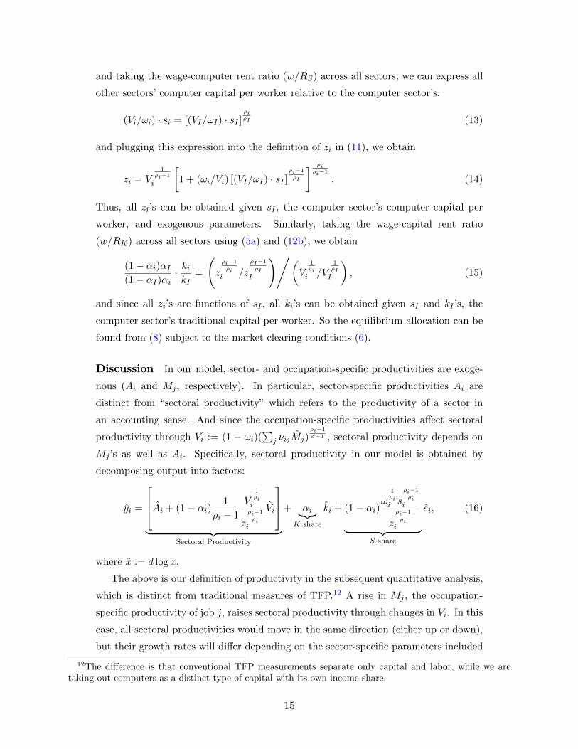
Discussion In our model, sector- and occupation-specific productivities are exoge-
nous (Ai and Mj , respectively). In particular, sector-specific productivities Ai are
distinct from “sectoral productivity” which refers to the productivity of a sector in
an accounting sense. And since the occupation-specific productivities affect sectoral
productivity through Vi := (1 − ωi)(∑
j νijMj)ρi−1
σ−1 , sectoral productivity depends on
Mj ’s as well as Ai. Specifically, sectoral productivity in our model is obtained by
decomposing output into factors:
yi =
Ai + (1− αi)1
ρi − 1
V1ρii
zρi−1
ρii
Vi
︸ ︷︷ ︸
Sectoral Productivity
+ αi︸︷︷︸K share
ki + (1− αi)ω
1ρii s
ρi−1
ρii
zρi−1
ρii︸ ︷︷ ︸
S share
si, (16)
where x := d log x.
The above is our definition of productivity in the subsequent quantitative analysis,
which is distinct from traditional measures of TFP.12 A rise in Mj , the occupation-
specific productivity of job j, raises sectoral productivity through changes in Vi. In this
case, all sectoral productivities would move in the same direction (either up or down),
but their growth rates will differ depending on the sector-specific parameters included
12The difference is that conventional TFP measurements separate only capital and labor, while we aretaking out computers as a distinct type of capital with its own income share.
15

Industry BEA industry code
Mining 211, 212, 213Construction 23Durable goods manufacturing 311FT, 313TT, 315AL, 322, 323, 324, 325, 326Non-durable goods manufacturing 321, 327, 331, 332, 333, 335, 3361MV, 3364OT, 337, 339FIRE 521CI, 523, 524, 531, 532RLHealth 621, 622HOOther high-skill services 512, 513, 514, 5411, 5412OP, 5415, 55, 61Trade (Retail & Wholesale) 42, 44RTOther low-skill services 22, 481, 482, 483, 484, 485, 486, 487OS, 493, 561, 562, 624,
711AS, 713, 721, 722, 81
Computer 334, 511
Table 1: Industry classificationRefer to BEA Industry Accounts for names of industries. The computer industry comprises hardware(computer and electronic products) and software (publishing industries).
in the expression for sectoral productivity in (16), as well as the endogenous response of
zi. And since the production technology is homogeneous of degree one (HD1), aggregate
productivity is a sectoral output-weighted average of the sectoral productivities. Hence
changes in the exogenous productivities Ai or Mj affect aggregate productivity both
directly by changing all sector’s sectoral productivities, but also indirectly by altering
sectoral output shares.
Last but not least, changes in AI , the computer industry’s sector-specific productiv-
ity, has further repercussions on aggregate output. As other industries, changes in AI
alter aggregate productivity both directly (by increasing the computer sector’s sectoral
productivity) and indirectly (by altering the output share of the computer industry).
But in addition, it lowers the price of computers (pI) and consequently the rental rate
of computer capital (RS), leading to a rise in the use of computers for industries whose
elasticity of substitution between computers and labor (ρi) is larger than one. Conse-
quently, not only because it raises aggregate productivity, but also because it increases
the use of computers in all sectors, a rise in AI contributes more to an increase in
aggregate output than any other sector-specific productivity does.
4 Quantitative Analysis
For the quantitative analysis, we classify industries into ten groups as summarized in
Table 1. We exclude the agricultural sector and government. In Table 2, we classify
occupations into ten groups which broadly correspond to one-digit occupation groups
in the census. We then fit the model exactly to the data for 1980, and let only the
16

Occupation Occupation code
High skillManagement 4 - 37Professionals 43 - 199
Middle skillMechanics & Construction 503 - 599Miners & Precision workers 614 - 699Technicians 203 - 235Sales 243 - 283Transportation 803 - 889Machine operators 703 - 799Administrative support 303 - 389
Low skill services 405 - 498
Table 2: Occupation classificationConsistent occupation code (occ1990dd) constructed following Autor and Dorn (2013).
exogenous occupation- and sector-specific productivities (Mj , Ai) grow at a constant
rate. Thus, a major test of the model is how well it replicates the data in 2010, or
equivalently, the growth of sectoral and aggregate variables from 1980 to 2010.
4.1 Calibration
Aggregate production function The parameters of the final good production
function are estimated outside of the model using real and nominal value-added data
by industry. Specifically, we estimate the sectoral weights γi and complementarity
parameter ε from
log(piYi/pIYI) =1
ε(γi/γI) +
ε− 1
εlog(Yi/YI), for i = 1, · · · , I − 1.
This system of equations is estimated by iterated feasible generalized nonlinear least
squares method. To reflect constraints on the parameters (ε > 0 and 0 < γi < 1), we
estimate the unconstrained coefficents b and ci’s in
log(pi,tYi,t/pI,tYI,t) = (1 + eb)ci + eb log(Yi,t/YI,t) + εi,t,
where ε = 1/(1 + eb) and γi = eci/(1 +∑eci).
Each sector i in the model consists of several industries in the BEA Industry Ac-
counts, to which we apply the Tornqvist index to obtain the price index of sector i.
Real quantities Yi are similarly aggregated up from the detailed BEA data. The ag-
gregate price index is normalized to 1 in 1963, the initial year in the data. The sample
17

Table 3: Estimation results
Parameters Estimates
ε 0.765∗∗∗
(0.002)
γ1 0.084∗∗∗
(0.001)γ2 0.159
∗∗∗(0.002)
γ3 0.099∗∗∗
(0.003)γ4 0.124
∗∗∗(0.002)
γ5 0.142∗∗∗
(0.001)γ6 0.087
∗∗∗(0.002)
γ7 0.057∗∗∗
(0.002)γ8 0.094
∗∗∗(0.003)
γ9 0.117∗∗∗
(0.002)
AIC -1001.432
Standard errors in parentheses.∗p < 0.10,
∗∗p < 0.05,
∗∗∗p < 0.01
period for the estimation covers 1980 to 2010, which is our main interest. The point
estimates for ε and γi are presented in Table 3.
Parameters calibrated without simulation In the calibration, we fix the tra-
ditional capital share of only the computer industry (αI) from the data. Though com-
puting the total capital share is straightforward (i.e., 1 minus labor share), computing
the traditional capital share according to our model is not. To obtain this number for
the computer industry, we follow Koh et al. (2016), which we briefly describe below.
We begin by specifying an empirical no-arbitrage condition for rental prices. The
return on both types of capital must be equal to the interest rate 1 + r′, so
[R′K + (1− δ′K)p′K ]/pK = [R′S + (1− δ′S)p′I ]/pI (17)
where pK is the price of traditional capital and pI the price of computers. Note that
this is different from the model’s no-arbitrage condition (7) in that we have included
the price of capital, which in the model we had normalized to be equal to the price of
the final consumption good. Next, since sectoral production is HD1 in all factor inputs
(traditional and computer capital, and labor), for the computer industry we have
1− labor shareI =RKKI
pIYI+RSSIpIYI
.
We solve for RK and RS from these two equations assuming a steady state (R′K =
RK , R′S = RS and pK = p′K , pI = p′I), plugging in for all other variables using data on
the quantities, prices and depreciation rates of each type of capital (from BEA FAT
Nonresidential Estimates by Industry and Type); and the computer industry’s real and
18

Parameters Value Obtained from
σ 0.815 Mean absolute distance of the changes in the employment sharer + δS 0.300 Average depreciation rate of computer capital from FAT
Table 4: Calibrated Parameters
nominal value-added, and its labor share (from BEA Industry Accounts).13 Once we
know RS , we can set αI = RSSI/pIYI since all other variables are recovered directly
from the data. We rely only on data from 1980.
Although the above procedure can be used for all industries, in our calibration
we only use it to compute the computer industry’s traditional capital share. All other
industries’ traditional capital shares are calibrated directly from the model as explained
below. Appendix Figure 17(a) compares the traditional capital shares obtained using
the above procedure against those predicted by the calibration, which confirms that
they are generally consistent.
Method of Moments The rest of parameters are recovered from simulating model
moments to match corresponding data moments. To be precise, we plug the data for Lij
(from the IPUMS Census), and (ki, si) (from the BEA FAT Nonresidential Estimates
by Industry and Type) directly into the equilibrium equations, assuming a steady state
in both 1980 and 2010, respectively. The detailed procedure is as follows:
1. Guess σ.
(a) Fix αI as above, and guess AI,1980 and ρi’s.
i. For 1980: obtain (νij , ωi, αi, Ai,1980) given guess.
- Normalize Mj = 1 for all j. Then the industry-specific occupation
weights νij ’s and Vi are recovered from (9)-(10) using data on 1980
employment shares..
- From (12a) of industry I, and replacing for yi using (1) and zi using
(11), ωI must solve
RS = (1−αI)·AIkαII ·
[ω
1ρII s
ρI−1
ρII + (1− ωI)
1ρI V
ρI−1
ρII
] 1−ρIαIρI−1
·(ωI/sI)1ρI ,
given data on kI and sI in 1980. The solution ωI ∈ (0, 1) if 1 <
(1− αI)AI(kI/sI)αI .13 We take the weighted average across industries 334 and 511 (software and hardware) to obtain this value
for the computer industry, which in our quantitative model comprises both. For each industry, computercapital is the sum of the net stock of “computers and peripheral equipment” and “software.”
19

- Given ωI , obtain all other ωi’s from (13) (since V := (1− ωi)V ρi−1i ).
- For all i 6= I, compute αi’s from (15) by replacing for zi using (14),
and plugging in data on (ki, si).
- Exogenous sector-specific productivities Ai,1980’s are recovered from
(8) and AI,1980.
ii. For 2010: obtain Mj,2010 and updated guesses for the substitutability
between computers and workers, ρnewi .
- Choose the Mj ’s that yields the best fit of (10) across all i given 2010
employment shares:
Mj
M1=
[∑i
(Li ·
LijLi1· νi1νij
)]/∑i
Li,
Using this we can compute Vi for 2010 using (9).
- From (15), we set ρnewI to get the best fit of
ρnewI ·I =∑i
log(ωI VI)− log((1− ωI)sI)
log[(
1− αI(1−αi)kiαi(1−αI)kI
)VI
]− log
(sIαI(1−αi)kiαi(1−αI)kI − si
)
given data on (ki, si) in 2010.
Note that we need si/sI < (1−αi)αIki/(αi(1−αI)kI) < 1 or si/sI >
(1 − αi)αIki/(αi(1 − αI)kI) > 1 for ρnewI to be a real number. We
exclude those industries with (ki, si) for which this condition is not
satisfied only when we compute ρnewI .
- Compute the implied ρnewi ’s that are consistent with the 2010 si’s, i.e.,
ρnewi =ρnewI log
(1−ωiωisiVi
)ρnewI log
(VIVi
)+ log
(1−ωIωIsI VI
)(b) Iterate over ρi’s till ρi ≈ ρnewi .
(c) Set AI,1980 so that yI equals the computer industry’s real value-added per
worker in the data. Iterate over AI,1980 till convergence.
2. Iterate over σ to minimize∑
j |`dj,2010− `mj,2010|, where `j is the employment share
of occupation j.
In the outermost loop of the above procedure, note that we use occupation employment
shares in aggregate. The industry-specific occupation weights νij ’s were recovered only
from within industry employment shares by occupation. Once we have recovered all
the parameters,
20
1. Get Ai,2010’s to match measured productivity by sector in (16) to 2010 data.14
2. Between 1980 and 2010, we assume that the Mj,t’s, and all Ai,t’s except AI , grow
at constant rates, so:
Mj,t = Mj,1980(Mj,2010/Mj,1980)(t−1980)/30,
Ai,t = Ai,1980(Ai,2010/Ai,1980)(t−1980)/30.
3. The computer sector’s exogenous productivity (AI) for other years are chosen so
that the sectoral productivity of the computer sector in (16) is equal in the data
and model.
4.2 Properties of the Benchmark Model
The calibration results are summarized in Tables 5 to 7. Since changes in Mj affect
occupational employment across all industries, we can identify occupation-specific pro-
ductivities separately from the sector-specific productivities. Specifically, occupational
employment data alone gives enough information to identify the Mj ’s, from Equa-
tion (10). Given this, we can identify the sector-specific Ai’s to fit measured sectoral
productivities from the data using (16). The calibrated values for Mj ’s show that
routine intensive occupations, such as machine operators or mechanics, indeed experi-
enced much faster growth in their occupation-specific productivities. And as expected,
the sector-specific productivity of the computer industry (AI) grew exceptionally fast
especially during the 1990s.
It is also noteworthy that the ρi’s are identified from how computer capital per
worker (si) and traditional capital per worker (ki) evolve differently across industries.
Roughly speaking, when an industry that increases computers per worker more than
other industries also uses more traditional capital per worker, the elasticity of substi-
tution ρi tends to be greater than one (Equation 15). But since traditional capital is a
constant share of production in our model, our model admits ρi > 1 for sectors whose
output per worker increases with computers per worker. Since this is indeed the case
for most industries in the data, as we saw in Figure 5, all calibrated ρi’s are larger than
1.15 This also implies that computerization leads to a decline in the labor share both
at the sector and aggregate levels.
In turn, sectors with higher computer per worker growth would also have higher
values of ρi, as in Figure 6. This is illustrated in Figure 6(a), which plots computer
14We compute traditional and computer capital income shares, and measure sectoral productivity directlyfrom the data. Hence, the model’s sectoral output may differ from the data.
15Figure 5 shows that some small industries have a negative relationship in the data, but this is no longerthe case once we aggregate the 60 industries into 10 more broadly defined sectors.
21

1.3 1.4 1.5 1.6 1.7 1.8 1.9 20.12
0.13
0.14
0.15
0.16
0.17
0.18
0.19
ρi
Com
pute
r pe
r C
apita
Gro
wth
(a) Data against computer-worker substitutability ρi
Cons FIRE Hlth Hser Lser ManD Mine M−ND Trad Comp10
11
12
13
14
15
16
17
18
19
20
DataModel
(b) Computer capital per worker
Fig. 6: Computer per worker growth between 1980 and 2010Source: BEA Industry Accounts and FAT. See Table 1 for details of the industry classification. Computercapital is measured as the sum of “computers and peripheral equipment” and “software” by industry, availablein FAT Table 3.1.
Param/Target Const FIRE HealthHighserv.
Lowserv.
Dur MineNon-durable
TradeComp-uter
γ outside 0.084 0.159 0.099 0.124 0.142 0.087 0.057 0.094 0.117 0.037ρ si,2010 1.699 1.213 1.413 1.461 1.415 1.263 1.445 1.559 1.419 1.840ω si,1980 0.001 0.094 0.003 0.025 0.006 0.028 0.020 0.009 0.008 0.020α ki,1980 0.167 0.374 0.301 0.454 0.475 0.333 0.793 0.402 0.186 0.322
Table 5: Industry specific parametersIndustry weights γi and the computer industry’s traditional capital income share αI are estimated directlyfrom the data using the BEA Industry Accounts and FAT, while the rest are calibrated according to amethod of moments. See text for details.
per worker growth in the data against the ρi’s. While panel (a) makes it clear how the
relative values of ρi are identified across sectors, note that the relationship is not exactly
linear, even though the model fits computer capital per worker exactly by assumption
as shown in panel (b)—since their empirical values are directly fed into step 1.ii of our
calibration. This is because computers are not substituting labor directly, but only
indirectly through the occupation composite Xi.16
16Related, since computers substitute a composite of labor rather than each occupation separately, thevalues of the substitutability parameters ρi’s are potentially sensitive to σ, which measures the complemen-tarity across occupations. We find that this is not the case for a wide range of values for σ lower than itsbenchmark value, as shown in Appendix Table 8. While ρi’s are sensitive to much larger values of σ, thenit becomes impossible to fit other moments in the data (employment shares and TFP by industry).
22

L serv. Admin. Mach Sales Trans Tech Mech Mine. Prof. Mngm
Const 0.009 0.058 0.027 0.009 0.218 0.016 0.564 0.015 0.021 0.061FIRE 0.048 0.444 0.005 0.225 0.015 0.014 0.013 0.004 0.021 0.211Health 0.328 0.172 0.005 0.004 0.006 0.122 0.009 0.011 0.293 0.050H serv. 0.109 0.222 0.010 0.020 0.022 0.043 0.037 0.007 0.420 0.110L serv. 0.375 0.143 0.025 0.041 0.129 0.012 0.080 0.023 0.070 0.101Durable 0.022 0.115 0.372 0.021 0.102 0.027 0.081 0.136 0.049 0.076Mining 0.017 0.103 0.047 0.010 0.195 0.051 0.121 0.311 0.065 0.080Non-dur 0.028 0.118 0.386 0.039 0.135 0.023 0.050 0.106 0.036 0.079Trade 0.025 0.150 0.022 0.406 0.152 0.005 0.066 0.042 0.022 0.110Computer 0.016 0.165 0.310 0.059 0.042 0.062 0.041 0.070 0.124 0.111
Table 6: Industry-occupation specific weights on labor (νij)Calibration results for νij from a method of moments. Empirical targets are within-industry employmentshares by occupation in 1980.
Target: emp. share by ind. and occ. in 2010 Target: measured productivity in 1980 and 2010Mj 1980 1990 2000 2010 Ai 1980 1990 2000 2010
Low serv. 1.000 1.000 1.000 1.000 Const 14.125 10.394 7.648 5.628Admin. 1.000 1.384 1.914 2.649 FIRE 17.924 17.267 16.633 16.023Machine 1.000 2.273 5.168 11.749 Health 6.155 6.460 6.780 7.115Sales 1.000 0.590 0.348 0.205 High serv. 1.385 1.624 1.904 2.232Trans 1.000 1.263 1.595 2.014 Low serv. 0.050 0.053 0.057 0.060Tech 1.000 0.736 0.542 0.399 Durable 0.198 0.191 0.185 0.179Mechanics 1.000 1.610 2.591 4.171 Mining 3.048 3.104 3.161 3.219Mine. 1.000 1.444 2.085 3.010 Non-durable 0.701 0.708 0.716 0.724Prof. 1.000 0.553 0.306 0.169 Trade 0.269 0.373 0.516 0.714Mngm 1.000 0.461 0.212 0.098 Computer 1.945 3.667 13.624 26.618
Table 7: Occupation- and sector-specific productivityOccupation-specific productivities are normalized to 1 in 1980. For 2010, we minimize the distance betweenthe model and data on within-industry employment shares by occupation averaged across all industries inthe IPUMS Census. The computer industry’s 1980 sector-specific productivity is chosen to minimize thedistance between model and data on its real value-added per worker in the BEA Industry Accounts, whileall other industries’ productivities are implied by the model and data on capital and labor data relativeto the computer sector from the Industry Accounts and FAT. All sector-specific productivities in 2010 arerecovered from our expression for sectoral productivity in (16), using the Industry Accounts data and ourcalibrated parameters. Except for the computer sector-specific productivity AI , all Ai’s are assumed to growat a constant rate from 1980 to 2010.
23

Low Admin Mach Sale Tran Tech Mech Mine Prof Mngm−0.25
−0.2
−0.15
−0.1
−0.05
0
0.05
0.1
0.15
0.2
0.25
DataModel
(a) By occupation
Cons FIRE Hlth Hser Lser ManD Mine M−ND Trad Comp−0.4
−0.3
−0.2
−0.1
0
0.1
0.2
0.3
DataModel
(b) By industry
Fig. 7: Changes in employment shares between 1980 and 2010Data Source: occupation data are from IPUMS Census, and industries from BEA Industry Accounts. SeeTable 2 for details of the occupation classification.
Model Fit The model-implied employment share changes fit the data better by
occupation than by industry (Figure 7). This is because the Mj ’s directly affect oc-
cupational employment through (10), and once we match sectoral productivity growth
by industry using (16), employment by industry is pinned down by (8).
This is also an indirect consequence of assuming constant σ’s across all industries.
Note that nowhere in our calibration did we separately target 2010 traditional capital
per worker, nor employment share changes by industry. Our calibration step 1.ii and
Equation (15) exploit all three factors at once, per industry, using only data on 2010
computer capital per worker by industry. This makes it clear that we can only let one
of ρ or σ vary by sector.17 Both would affect how factor input ratios, and in particular
computer capital per worker si, change across sectors in response to changes in Mj ’s.
But one of our major goals is to quantitatively compare how aggregate productivity
is affected by complementarity across occupations (shifts in Mj through σ) relative to
complementarity across industries (shifts in Ai through ε). How to implement such a
comparison becomes less obvious if σ’s vary across sectors.
More important, letting the elasticity of substitution between computers and labor
(ρi) vary across sectors directly captures how computer capital per worker evolves
differentially across sectors, as we discussed above. If we were to instead let σ vary, the
effect is only indirect since computer-labor substitution would differ across sectors only
due to differential shifts in relative labor demand. That is, unlike the clear relationship
17Since the Vi’s are functions of σ.
24

Cons FIRE Hlth Hser Lser ManD Mine M−ND Trad Comp−2
0
2
4
6
8
10
12
14
DataModel
(a) Output per worker
Cons FIRE Hlth Hser Lser ManD Mine M−ND Trad Comp−1
0
1
2
3
4
5
DataModel
(b) Tradition capital per worker
Fig. 8: Log changes of y and k between 1980 and 2010Data Source: BEA Industry Accounts and FAT. See Table 1 for details of the industry classification.
between ρi and the growth of computer per worker si as seen in Figure 6(a), there
would be no systematic relationship between σ and si since it would also depend on
the sector-specific occupation weights νij ’s.
Thus, our exact fit to computer capital per worker growth, to some extent, comes
at the expense of a lesser fit to employment share changes and traditional capital
per worker growth by industry. See Figures 7(b) and 8(b). This indicates that the
unit elasticity assumption between traditional capital and other factors, and also the
assumption that the elasticity is constant across sectors, may be too stringent. Still,
both changes in employment shares and traditional capital per worker by industry are
qualitatively consistent with the data.
More assuringly, even though we did not use any data on output per worker
growth—neither by industry nor in aggregate—nor aggregate productivity, the model
prediction of output per worker growth by industry is remarkably close to the data,
Figure 8(a). Most importantly for our purposes, the model generates a slowdown in
aggregate output and productivity growth starting in 2000, similarly as in the data, as
shown in Figure 9 and tabulated in Appendix Table 9. The fit to aggregate productiv-
ity is especially remarkable considering that we assume constant productivity growth
rates for Mj and Ai—other than AI—and do not target any aggregate variables in
2010.
Lastly, the model-implied factor income shares by industry are also generally con-
sistent with the data (Appendix Figure 17). Partly because of this, the aggregate
25

1980 1990 2000 2010 2015−0.2
0
0.2
0.4
0.6
0.8
1
1.2
ModelData
(a) Output
1980 1990 2000 2010 2015−0.1
−0.05
0
0.05
0.1
0.15
0.2
0.25
0.3
ModelData
(b) Productivity
Fig. 9: Aggregate productionData Source: BEA NIPA. Exact numbers for the plots are tabulated in Appendix Table 9.
labor share in the model closely tracks the trend in the data, both in direction and
magnitude (Figure 10), despite not being targeted at all at the sectoral nor aggregate
levels. Recall that our production technology assumes that traditional capital’s income
share is constant by construction. Thus, our results suggest that computer hardware
and software, which are a subset of total capital that accounts for 14 percent of all
investment, can be responsible for the vast majority of the fall in the labor share (4
out of 5 percentage points) since 1980.18
4.3 Counterfactual Analysis
In this section, we investigate the underlying factors that shape aggregate output
and productivity, focusing on routinization and computerization. Routinization in our
model is a faster increase in the occupation-speciifc productivity, Mj , of certain occu-
pations. Computerization is driven by the computer industry-specific term, AI , which
propagates through all industries because computer capital is used in the production
of all industrial goods.
In our model equilibrium, this propagation happens by shifting the price of com-
puter capital. High AI shrinks the computer sector employment because of comple-
mentarity, but also lowers the relative price of computers. This, in turn, leads to a drop
in the rental rate of computer capital, which induces all sectors to use more computers.
18As a direct consequence of not fitting capital per worker growth by sector, the model fit to the fall inlabor shares by sector is poorer than in aggregate. Aggregate capital per worker k in the data is directly fedinto the model.
26

1980 1990 2000 2010 20150.53
0.54
0.55
0.56
0.57
0.58
0.59
0.6
0.61
ModelData
(a) Aggregate
Cons FIRE Hlth Hser Lser ManD Mine M−ND Trad Comp−1
−0.8
−0.6
−0.4
−0.2
0
0.2
0.4
DataModel
(b) By industry
Fig. 10: Changes in labor share: model vs. dataData Source: BEA NIPA and Industry Accounts. See Table 1 for details of the industry classification.
This prevents the computer sector from shrinking.
Aggregate productivity Note that the growth rates of occupation- and sector-
specific productivities (Mj and Ai) were assumed to be constant for the entire sample
period except for the computer sector’s (AI). Nonetheless, in the benchmark calibra-
tion, aggregate TFP increases almost linearly from 1980 to 2000, slowing down in the
last decade (Figure 11).19 We now show that the high growth rate of the computer
sector-specific productivity (AI) prevented a potential slowdown in aggregate produc-
tivity that would have appeared between 1990 and 2000. Figure 11 shows that, if we
assume AI were constant between 1980 and 2010, aggregate productivity growth would
have slowed down since 1990. Without the growth in AI , aggregate productivity would
have grown by only 13 percent from 1980 to 2010, one-third lower than the benchmark
growth rate of 20 percent over the same period. This magnitude is surprising consider-
ing the fact that the computer sector’s share of aggregate output is only 3 to 4 percent
throughout the observation period.
When all occupation- and sector-specific productivities grow at constant rates over
time, complementarity across jobs and sectors induces the faster growing jobs and
sectors to shrink in relative size, reducing their weights in the computation of aggregate
productivity. Hence, as long as occupation- and sector-specific productivities grow at
different rates, aggregate productivity growth must slow down over time. So both the
19Aggregate productivity growth is measured as d log(y) − (traditional capital share) · d log(k) −(computer share) · d log(s).
27

1980 1990 2000 20100
0.02
0.04
0.06
0.08
0.1
0.12
0.14
0.16
0.18
0.2
benchmarkno computerization
(a) Log level
1980−1990 1990−2000 2000−20100.1
0.2
0.3
0.4
0.5
0.6
0.7
0.8
0.9
benchmarkNo computerization
(b) Growth rate
Fig. 11: Aggregate Productivity without Computerization
dispersions in the growth rates of occupation-specific productivities (Mj) and in sector-
specific productivities (Ai’s) contribute to the aggregate productivity slowdown. To
find out which dispersion is more important for the slowdown, we conduct the following
exercises.
In the first exercise, we force all Mj ’s to grow at the same rate m for all j (i.e., no
routinization) while leaving the growth rates of Ai’s to be different from one another
as in the benchmark. Second, we force all Ai’s to grow at a common rate a while
leaving the growth rates of Mj ’s heterogeneous as in the benchmark. The common
growth rates m and a are set so that aggregate productivity grows at the same rate
as in the first decade of our benchmark calibration. The results are shown in Figure
12, which shows that routinization, or the dispersion in the growth rates of Mj , is
more important in explaining the decline in the growth rate of aggregate productivity.
Without routinization, the growth rate of aggregate productivity remains near 0.8
percent per year throughout the three decades. In contrast, even when all sector-
specific productivities grow at a common rate, aggregate productivity growth falls
almost as much as in the benchmark. Of course for the latter exercise, we are also
ruling out the faster growth of the computer sector, which partially explains the gap
between the benchmark growth rate and this counterfactual growth rate in the 1990s.
Output Fast-growing computer sector-specific productivity directly boosts aggre-
gate productivity, which leads to an acceleration of aggregate output growth. Fur-
thermore, there is an additional effect on aggregate output, since all sectors use more
computer capital. Figure 13 shows the total effect of computerization on aggregate
28

1980 1990 2000 20100
0.05
0.1
0.15
0.2
0.25
benchmarkcommon mcommon a
(a) Log level
1980−1990 1990−2000 2000−2010
0.4
0.5
0.6
0.7
0.8
0.9
1
benchmarkcommon mcommon a
(b) Growth rate
Fig. 12: Aggregate Productivity without Complementarity
1980 1990 2000 20100
0.1
0.2
0.3
0.4
0.5
0.6
0.7
0.8
0.9
benchmarkno computerization
(a) Log level
1980−1990 1990−2000 2000−20100
0.5
1
1.5
2
2.5
3
3.5
4
benchmarkNo computerization
(b) Growth rate
Fig. 13: Aggregate Output without Computerization
29

Comp FIRE Hser Mine ManD M−ND Lser Trad Hlth Cons0
2
4
6
8
10
12
Databenchmarkno computerization
Fig. 14: Output Growth by Industry without ComputerizationIn panel (a), we plug in model-simulated income shares and quantities into the accounting equations in(18). In panel (b), we plug in data from NIPA and FAT directly. See Table 1 for details of the industryclassification.
output. If AI were to remain constant between 1980 and 2010, aggregate output
growth from 1980 to 2010 would be 63 percent, or only about half of the growth in the
benchmark. As expected, this is a larger impact than that on aggregate productivity.
Figure 14 shows output growth by industry with and without AI growth. Due to
the substitutability between computer and labor, all industries benefit from computer-
ization. Unsurprisingly, the computer industry itself is affected the most, followed by
finance and high-skilled services. The construction industry has the least to gain (in
terms of output growth) from computerization.
Labor share Because the model calibration yields sector-specific elasticities of sub-
stitution between labor and computer capital (ρi) that are larger than 1, computer-
ization results in the decline of labor shares in all sectors. Figure 15 shows changes
in labor shares by industry for various counterfactual exercises. Among all these ex-
ercises, the only two that affect labor shares are when we eliminate computerization
either explicitly (in red); or by assuming common growth rates across all industries
(in sky-blue). So we can conclude that the growth in AI is the only important driving
force behind the decline of the labor share.
30

Cons FIRE Hlth Hser Lser ManD Mine M−ND Trad Comp−1
−0.8
−0.6
−0.4
−0.2
0
0.2
0.4
Databenchmarkno compcommon mcommon a
Fig. 15: Changes in Labor Income Shares by Industry“no comp”: no computerization. “common m”: no complementarity across jobs. “common a”: no comple-mentarity across industries. See Table 1 for details of the industry classification.
Computer capital in the measurement of TFP In our benchmark, we mea-
sured aggregate productivity growth between times s and t as follows:
log(At/As) = log(Yt/Ys)−1
2
(LItYt
+LIsYs
)log(Lt/Ls)−
1
2
(SItYt
+SIsYs
)log(St/Ss)
− 1
2
(KItYt
+KIsYs
)log(Kt/Ks), (18a)
where LI is labor income, SI is computer capital income, and KI is traditional capital
income. But typically, the standard way we compute TFP growth (the Solow residual
A) is
log(At/As) = log(Yt/Ys)−1
2
(LItYt
+LIsYs
)log(Lt/Ls)
− 1
2
(KIs + SIt
Yt+KIs + SIs
Ys
)log[(Kt + St)/(Ks + Ss)]. (18b)
Note that At and At can differ, especially when the gross rate of return on computer
capital and traditional capital are different. By inspection of (17), we see that this
happens when either the investment prices and/or the depreciation rates of the two
types of capital differ. In particular, the gross rate of return on computer capital is
generally higher than traditional capital because the former depreciates more quickly.
This implies that the standard way of computing TFP without separating out computer
capital will overestimate the growth rate of aggregate productivity.
31

1980 1990 2000 20100
0.05
0.1
0.15
0.2
0.25
0.3
0.35
BenchmarkTotal K
(a) Model
1980 1990 2000 2010 2015−0.1
−0.05
0
0.05
0.1
0.15
0.2
0.25
0.3
0.35
BenchmarkTotal K
(b) Data
Fig. 16: Comparing different measures of TFP’sIn panel (a), we plug in model-simulated income shares and quantities into the accounting equations in (18).In panel (b), we plug in data from NIPA and FAT directly.
In Figure 16, we compare aggregate productivity from our benchmark calibration
(A) against the TFP (standard Solow residual, A), both according to our model (panel
a) and in the data (panel b). For panel (a), we plug in our model-simulated data into
(18). For panel (b), we impute all variables needed in (18) directly from the data. The
figure confirms that the aggregate productivity growth is overestimated by about 10
percentage points over the past 30 years if computer capital is not explicitly separated,
both in the data and also according to our model.
Summary of quantitative analysis There are two main findings from our quan-
titative analysis. First, constant occupation- and sector-specific technological progress
necessarily slows down aggregate productivity growth over time, given complementar-
ity across jobs and industries. Second, it was the dispersion in the growth rates across
occupations (i.e., routinization) that was most responsible for the aggregate produc-
tivity slowdown. This negative impact of routinization on the growth rate of aggregate
productivity was more or less perfectly counterbalanced by the impressive technologi-
cal progress specific to the computer industry and its spillover through inter-industry
linkages during the 1980s and the 1990s. The slower pace of the computer sector’s pro-
ductivity growth in recent years—and the associated deceleration of computer usage
by other industries since 2000—is finally revealing the negative impact that decades of
routinization has had on aggregate productivity growth.
32

5 Concluding Remarks
We presented a model in which productivities grow at heterogeneous rates across oc-
cupations (routinization), and also across industries. In particular, to understand the
effect of the rise of the computer industry on aggregate productivity, we let its output
be used in the production of all industries as a distinct type of capital.
We showed that when occupations and industries are complementary to one another
and occupation- and sector-specific productivities grow at different rates, routinization
in particular causes a slowdown in aggregate productivity. But such a slowdown was
averted prior to the 2000s in the U.S., thanks to the rapid rise of the computer indus-
try’s productivity. It was only after the productivity of this sector slowed down that
routinization began to reveal its negative impact on aggregate productivity growth.
The main message of our model is that multiple layers of the economy (i.e., occu-
pations and sectors) can interact to generate interesting time trends that can help us
reconcile evidence at the occupation and sector levels with aggregate trends. More-
over, we have also highlighted the importance of inter-industry linkages by showcasing
that a single industry—in our case the computer industry—can have large effects on
aggregate variables once such a propagation mechanism is taken into account.
In reality, all industries are interlinked, not only by providing intermediate inputs
to one another as emphasized in some recent models (Acemoglu, Carvalho, Ozdaglar,
and Tahbaz-Salehi, 2012; Atalay, 2017) but also by serving different types of capital in
which all industries need to invest (as we have modeled here). Modeling such additional
layers of complexity is left for future research.
References
Acemoglu, D., D. Autor, D. Dorn, G. H. Hanson, and B. Price (2014, May). Return
of the Solow paradox? IT, productivity, and employment in US manufacturing.
American Economic Review 104 (5), 394–99.
Acemoglu, D., V. M. Carvalho, A. Ozdaglar, and A. Tahbaz-Salehi (2012). The network
origins of aggregate fluctuations. Econometrica 80 (5), 1977–2016.
Atalay, E. (2017, October). How important are sectoral shocks? American Economic
Journal: Macroeconomics 9 (4), 254–80.
Aum, S. (2017). The rise of software and skill demand reversal. Manuscript.
33

Aum, S., S. Y. T. Lee, and Y. Shin (2017). Industrial and occupational employment
changes during the Great Recession. Federal Reserve Bank of St. Louis Review 99 (4),
307–317.
Autor, D. H. and D. Dorn (2013). The growth of low-skill service jobs and the polar-
ization of the US labor market. American Economic Review 103 (5), 1553–97.
Baumol, W. J. (1967). Macroeconomics of unbalanced growth: The anatomy of urban
crisis. The American Economic Review 57 (3), 415–426.
Byrne, D. M., J. G. Fernald, and M. B. Reinsdorf (2016). Does the United States
have a productivity slowdown or a measurement problem? Brookings Papers on
Economic Activity 47 (1 (Spring), 109–182.
Cortes, G. M., N. Jaimovich, and H. E. Siu (2017). Disappearing routine jobs: Who,
how, and why? Journal of Monetary Economics.
Duernecker, G., B. Herrendorf, and A. Valentinyi (2017). Structural change within the
service sector and the future of Baumol’s disease.
Goos, M., A. Manning, and A. Salomons (2014). Explaining job polarization: Routine-
biased technological change and offshoring. American Economic Review 104 (8),
2509–26.
Karabarbounis, L. and B. Neiman (2014). The global decline of the labor share. The
Quarterly Journal of Economics 129 (1), 61–103.
Koh, D., R. Santaeullia-Llopis, and Y. Zheng (2016, September). Labor share decline
and intellectual property products capital. Working Papers 927, Barcelona Graduate
School of Economics.
Lee, S. Y. T. and Y. Shin (2017). Horizontal and vertical polarization: Task-specific
technological change in a multi-sector economy. Technical Report Working Paper
23283, NBER.
Ngai, L. R. and C. A. Pissarides (2007, March). Structural change in a multisector
model of growth. American Economic Review 97 (1), 429–443.
Syverson, C. (2017, May). Challenges to mismeasurement explanations for the US
productivity slowdown. Journal of Economic Perspectives 31 (2), 165–86.
34

A Tables and Figures Not Included in Text
Const FIRE Health Highserv.
Lowserv.
Dur Mine Non-durable
Trade Comp-uter
σ = .1 1.577 1.260 1.497 1.579 1.447 1.222 1.423 1.462 1.505 1.828σ = .5 1.593 1.245 1.473 1.546 1.436 1.225 1.422 1.473 1.480 1.825σ = .7 1.624 1.229 1.444 1.506 1.423 1.234 1.426 1.498 1.451 1.825σ = .815 1.699 1.213 1.413 1.461 1.415 1.263 1.445 1.559 1.419 1.840
Table 8: Calibrated ρi’s across various σ’sFor each value of σ, the ρi’s are calibrated as explained in Section 4.1 except that σ is fixed. We found thatfor values of σ above its benchmark value of 0.815, the model fit quickly becomes exponentially poor with nosolution as it approaches 1. The reason is that occupation-specific productivities Mj become so large thatit becomes impossible to simultaneously match employment share changes and measured TFP by industry.
Output ProductivityData Model Data Model
1980- 3.41 3.81 0.43∗ 0.851990- 3.75 3.28 1.26 0.732000- 1.54 1.30 0.44 0.34
Table 9: Model Fit to Aggregate Output and ProductivityData source: BEA NIPA. ∗Although average productivity growth seems low in the data for the 1980s, thisis more of a cyclical phenomena in the early 1980s that persisted from the late 1970s. For example, averageproductivity growth from 1982-1990 is 1.18%.
35

0 0.2 0.4 0.6 0.8 10
0.1
0.2
0.3
0.4
0.5
0.6
0.7
0.8
0.9
Data
Mod
el
(a) Traditional Capital share
0 0.2 0.4 0.6 0.8 10
0.1
0.2
0.3
0.4
0.5
0.6
0.7
0.8
0.9
Data
Mod
el
19802010
(b) Labor share
Fig. 17: Factor income shares by industry: model vs. dataIn the model, traditional capital income shares are computed by first fixing that of the computer industry’sto 1980 data as explained in Section 4.1, and then calibrating them for all other industries using a methodof moments. Data traditional capital income shares are computed by applying the procedure in Section 4.1too all industries in 1980. All data from BEA NIPA and FAT.
36