Centre forComputationalFinance andEconomicAgents

WorkingPaperSeries

WP071-13

Iacopo GiampaoliWing Lon Ng

Nick Constantinou

Periodicities of ForeignExchange Markets and the

Directional Change Power Law

2013

Periodicities of Foreign Exchange Markets and the

Directional Change Power Law

Iacopo Giampaoli ∗ Wing Lon Ng† Nick Constantinou ‡

April 11, 2013

Abstract

This paper utilises advanced methods from Fourier Analysis in order to de-

scribe periodicities in financial ultra-high frequent FX data. The Lomb-Scargle

Fourier transform is used to take into account the irregularity in spacing in

the time-domain. It provides a natural framework for the power spectra of dif-

ferent inhomogeneous time series processes to be easily and quickly estimated.

Furthermore, event-based approach in intrinsic time based on a power-law re-

lationship, is employed using different event thresholds to filter the foreign

exchange tick-data. The calculated spectral density demonstrates that the

price process in intrinsic time contains different periodic components for di-

rectional changes, especially in the medium-long term, implying the existence

of stylised facts of ultra-high frequency data in the frequency domain.

Keywords: Ultra-high frequency transaction data, foreign exchange, irregu-

larly spaced data, Lomb-Scargle Fourier transforms, spectral density.

JEL Classifications: C22, C58, C63.

∗Centre for Computational Finance and Economic Agents (CCFEA), University of Essex,Wivenhoe Park, Colchester CO4 3SQ, UK.†Corresponding author. E-mail: wlng@essex.ac.uk. Centre for Computational Finance

and Economic Agents (CCFEA), University of Essex, Wivenhoe Park, Colchester CO4 3SQ, UK.‡Essex Business School, University of Essex, Wivenhoe Park, Colchester CO4 3SQ, UK.

The authors are grateful to Richard Olsen for his valuable helpful discussion and to Olsen FinancialTechnologies for providing the FX market data.

1

1 Introduction

In financial markets, trading activity typically tends to vary depending on the time

of day, shrinking during lunch time and over weekends, and increasing prior to

major scheduled news announcements (see, for example, Chordia, Roll, and Subrah-

manyam, 2001). These observations are usually measured in physical time. Another

approach that has been recently put forward and which has led to a rich array of

scaling behaviour in FX market is a time scale that is defined via events, i.e. the so

called intrinsic time (see Derman, 2002; Glattfelder, Dupuis, and Olsen, 2011).

In particular, the presence of different patterns of trading activity in financial

markets makes the flow of physical time discontinuous, as the number of transactions

tends to increase or decrease at different time intervals. This empirical observation,

which led to the definition of intrinsic “trading time”, coined by Mandelbrot and

Taylor (1967), suggests that the concept of physical time may not be the fundamental

time scale and research should additionally focus on an event-based time scale. In

this paper, the analysis of price movements focuses on an intrinsic time scale defined

by “directional-change” events: price movements exceeding a given threshold which

are independent of the notion of physical time. Recent literature has demonstrated

a rich landscape of scaling laws in intrinsic time for “ultra-high-frequency” (UHF)

FX data (for an early survey, see Bouchaud (2001, 2002)), including a scaling law

for the directional-change events considered in this paper.

Following the intrinsic time paradigm by Glattfelder, Dupuis, and Olsen (2011),

we filter our UHF data by analysing those points where there has been a directional-

change (the event), consisting of price movements away from a local maximum

(or minimum), which exceed a given threshold (for a more formal description, see

Hautsch, 2004, p. 36). The newly created time series naturally includes fewer ob-

servations, but still contains significant information about the price evolution via

its associated scaling law and about the temporal structures through its directional-

change duration, and is irregular-spaced in time. Indeed, time series in intrinsic

2

time are fundamentally unevenly-spaced in time and there is no justification in ar-

tificially making them equally-spaced (see also Dacorogna, Gençay, Müller, Olsen,

and Pictet, 2001; Giampaoli, Ng, and Constantinou, 2009).

Aldridge (2010) argues that trading opportunities are indeed present at various

data frequencies (i.e. observation intervals), hence suggesting that agents with dif-

ferent time horizons and risk preferences would be able to trade profitably in the

market. One of the key features common to all types of high-frequency data is

the persistence of underlying trading opportunities: these range from fractions-of-a-

second price movements, arising from market-making trades, to several-minute-long

strategies based on momentum forecasted by microstructure theories, to several-

hour-long market moves deriving from cyclical events and deviations from statistical

relationships (Aldridge, 2010). The development of high-frequency trading strate-

gies begins with the identification of recurrent (i.e. periodic) profitable trading

opportunities present in the data, and their profitability depends upon the chosen

trading frequency. As the data frequency increases, the possible range of each price

movement shrinks, but the number of ranges increases, thus potentially increasing

trades profitability 1.

The main goal of this paper is to detect potential periodic patterns of UHF FX

market data. For example, it is well-known that intraday data have a consistent

diurnal pattern of trading activities over the course of a trading day due to insti-

tutional characteristics of organised financial markets, such as opening and closing

hours or intraday auctions. In fact, FX markets have stronger seasonal patterns as

they are open 24/7 and constantly influenced by re-occurring time-zone effects. (see

also Bauwens, Ben Omrane, and Giot, 2005; Ben Omrane and de Bodt, 2007).

In particular, this paper employs advanced modelling techniques from Fourier

analysis, which provide a natural framework to analyse inhomogeneous time series1In fact, Aldridge (2010) calculates the maximum gain as the sum of price ranges at each

frequency, whereas the maximum potential gain (loss) at every frequency is determined by the(negative) sum of all per-period ranges at that frequency.

3

in the frequency domain and also reduce the computational time needed to process

a large amount of transaction data. Fast Fourier transform (FFT) algorithms are

commonly used to analyse equally-spaced time series in the frequency domain, but in

their standard form, they require either regular resampling of the unevenly-spaced

data, or interpolating them onto an equally-spaced grid (Bisig, Dupuis, Impagli-

azzo, and Olsen, 2012). In fact, any such transformation via regular resampling of

unevenly-spaced data or interpolation to an evenly-spaced grid (in order to calculate

the SDF with the simple FFT), leading to loss of information and the use of spurious

information (Giampaoli, Ng, and Constantinou, 2009).

The Lomb-Scargle Fourier transform (LSFT), a generalisation of the discrete

Fourier transform, is especially designed for unevenly-spaced data and represents the

natural tool to study UHF data in the frequency domain as it allows the stochastic

behaviour of every single process to be determined without any loss of information.

The LSFT, in contrast to existing autoregressive conditional models (e.g., ACD

or ACI models) in the literature, has also the advantage of greatly reducing the

computational effort required when analysing UHF transaction data sets and of

avoiding complex model specifications or obligatory deseasonalisation. We apply

the LSFT to UHF FX series which are filtered by the directional change event and

hence satisfy a scaling law. The scaling law relates the directional change duration

in physical time (corresponding to one tick in intrinsic time) with the directional

change threshold.

The structure of this paper is organised as follows. Section 2 motivates and

introduces the methods employed in this study. Section 3 presents the empirical

data and the results. Section 4 concludes.

4

2 Method

Our analysis is made in the frequency domain of an intrinsic-time process defined

by a directional-change event. If the latter is governed by a scaling law, the filtered

time series would have certain characteristics of scale-invariance and proportionality,

even for its periodic patterns. In the following, Subsection 2.1 first describes the

adopted event-based approach and the resulting scaling law. The LSFT for the

spectral analysis of the UHF data is then introduced and defined in Section 2.2.

Our goal is to capture the scale invariant periodicity of the intraday price series;

i.e., for the same frequency in the spectral density of a directional change series

sampled with a higher threshold, one can also find a corresponding significant peak

in the spectral density sampled with a lower threshold - despite the irregular spacing

in (physical) time.

2.1 Intrinsic Time and Directional Changes

Directional changes of price dynamics are the main source of volatility. Historically,

the concept of directional change played an important role in technical analysis,

as turning points of fundamental price movements are used by intraday traders

to identify optimal times to buy or sell. For example, point-and-figure charting

techniques, reportedly in use from the late 19th century, track price changes of

fixed thresholds and significant price reversals, and are often employed to identify

price trends, support and resistance levels in intraday trading data (among the

oldest written references are Wyckoff, 1910 and deVilliers, 1933). Additionally, the

so called “directional change frequency”, which estimates the average number of

directional price changes of a given threshold over a data sample, can be interpreted

as an alternative measure of risk (Guillaume, Dacorogna, Davé, Müller, Olsen, and

Pictet, 1997).

Let x denote the price and ∆x the price change. In the event-driven setting

5

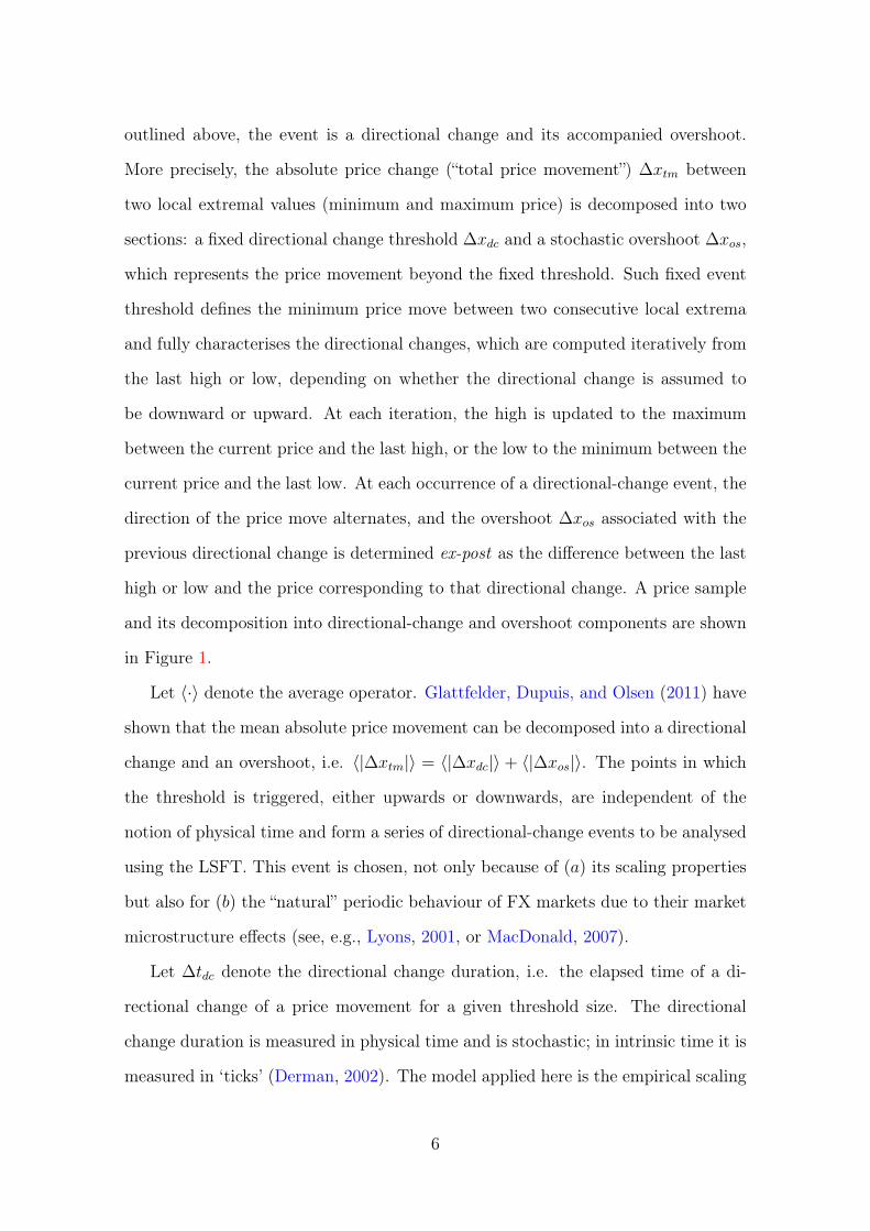
outlined above, the event is a directional change and its accompanied overshoot.

More precisely, the absolute price change (“total price movement”) ∆xtm between

two local extremal values (minimum and maximum price) is decomposed into two

sections: a fixed directional change threshold ∆xdc and a stochastic overshoot ∆xos,

which represents the price movement beyond the fixed threshold. Such fixed event

threshold defines the minimum price move between two consecutive local extrema

and fully characterises the directional changes, which are computed iteratively from

the last high or low, depending on whether the directional change is assumed to

be downward or upward. At each iteration, the high is updated to the maximum

between the current price and the last high, or the low to the minimum between the

current price and the last low. At each occurrence of a directional-change event, the

direction of the price move alternates, and the overshoot ∆xos associated with the

previous directional change is determined ex-post as the difference between the last

high or low and the price corresponding to that directional change. A price sample

and its decomposition into directional-change and overshoot components are shown

in Figure 1.

Let 〈·〉 denote the average operator. Glattfelder, Dupuis, and Olsen (2011) have

shown that the mean absolute price movement can be decomposed into a directional

change and an overshoot, i.e. 〈|∆xtm|〉 = 〈|∆xdc|〉 + 〈|∆xos|〉. The points in which

the threshold is triggered, either upwards or downwards, are independent of the

notion of physical time and form a series of directional-change events to be analysed

using the LSFT. This event is chosen, not only because of (a) its scaling properties

but also for (b) the “natural” periodic behaviour of FX markets due to their market

microstructure effects (see, e.g., Lyons, 2001, or MacDonald, 2007).

Let ∆tdc denote the directional change duration, i.e. the elapsed time of a di-

rectional change of a price movement for a given threshold size. The directional

change duration is measured in physical time and is stochastic; in intrinsic time it is

measured in ‘ticks’ (Derman, 2002). The model applied here is the empirical scaling

6

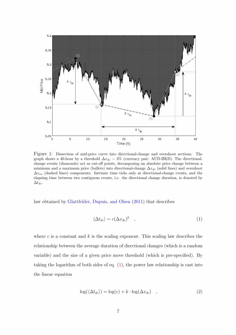
Figure 1: Dissection of mid-price curve into directional-change and overshoot sections. Thegraph shows a 40-hour by a threshold ∆xdc = 3% (currency pair: AUD-HKD). The directional-change events (diamonds) act as cut-off points, decomposing an absolute price change between aminimum and a maximum price (bullets) into directional-change ∆xdc (solid lines) and overshoot∆xos (dashed lines) components. Intrinsic time ticks only at directional-change events, and theelapsing time between two contiguous events, i.e. the directional change duration, is denoted by∆tdc.

law obtained by Glattfelder, Dupuis, and Olsen (2011) that describes

〈∆tdc〉 = c(∆xdc)k , (1)

where c is a constant and k is the scaling exponent. This scaling law describes the

relationship between the average duration of directional changes (which is a random

variable) and the size of a given price move threshold (which is pre-specified). By

taking the logarithm of both sides of eq. (1), the power law relationship is cast into

the linear equation

log(〈∆tdc〉) = log(c) + k · log(∆xdc) , (2)

7

characterised by the slope k and the intercept log(c). The scaling exponent k mea-

sures the proportional change of the average directional-change duration due to

an increment of the price threshold. Different directional-change threshold sizes

∆xdc = {10bp, 15bp, 20bp, 25bp, 30bp, 40bp, 50bp, 75bp, 100bp, 125bp, 150bp,

175bp, 200bp} are chosen to generate the respective average directional-change du-

rations for the individual sampling window. Standard linear OLS regression is used

to estimate the scaling law parameters in eq. (2); the results are presented in Section

3.

The objective of this work is to demonstrate that the use of LSFT within an

event-based framework reveals new periodic patterns in FX time series and provides

insightful information on the price process with respect to different threshold levels

and their corresponding seasonality. The cut-off points between each directional

change and the corresponding overshoot form a new event-based and irregularly-

spaced time series in intrinsic time (see Figure 1), which serves as input for the

LSFT to calculate the spectral density function (SDF). The LSFT framework is

described in the following section.

2.2 Spectral Analysis of Tick-Data

Spectral analysis decomposes a time series into its periodic frequencies in order to

detect and analyse its cyclical behaviour. The application of spectral techniques in

periodic economic processes has a long history, and a significant effort is employed

in the estimation of the spectral density function (SDF) (Priestley, 1981). The

SDF represents the analogue of the autocorrelation function in the time domain

and encapsulates the frequency properties of the time series determining how the

variation in a time series is built-up by components at different frequencies.

For standard periodic time series a FFT algorithm is generally employed to de-

termine their spectral properties (Priestley, 1981). As tick-by-tick data and the

resultant filtered time series in intrinsic time are unevenly-spaced, the traditional

8

FFT can not be applied without artificially tampering with the raw data (see also

Dacorogna, Gençay, Müller, Olsen, and Pictet, 2001; Bauwens, Ben Omrane, and

Giot, 2005; Ben Omrane and de Bodt, 2007). Attempts to transform the irregularly-

spaced raw data into regularly-spaced data, by regular resampling, averaging, or

using interpolation, prior to applying the FFT to calculate the SDF (e.g., Bisig,

Dupuis, Impagliazzo, and Olsen, 2012), has recently been demonstrated to cause

(a) loss of information, (b) generation of spurious data, or (c) both. It has also been

shown that these limitations can be overcome using the LSFT (see Giampaoli, Ng,

and Constantinou, 2009). Lomb (1976) first introduced this statistical method in as-

trophysics and fitted sinusoidal curves to the unevenly-spaced data by least-squares

in order to determine their periodic behaviour, despite the irregular spacing in time.

Scargle (1982) later developed the methodology further by deriving the standardised

Lomb-Scargle (LS) periodogram that has well defined statistical properties as the

work of Horne and Baliunas (1986) demonstrated.

Many diverse areas of science have tackled this issue using the robust framework

of the LSFT (for an overview, see Ware, 1998). Under this framework, the data on

the non-equally spaced grid is transformed into the frequency domain in order to

obtain an unbiased estimation of the SDF. The resulting SDF is calculated for k ∈

{1, 2, 3...,M} frequencies, with M chosen as outlined in Press, Flannery, Teukolsky,

and Vetterling (1992). Consider a signal x, observed a time tj, with mean x̄ and

variance σx. The normalised SDF is given by

SDFLS (ωk) =1

2σ2x

[∑N

j=1 (xj − x̄) cosωk (tj − τ)]2

∑Nj=1 cos2 ωk (tj − τ)

+

[∑Nj=1 (xj − x̄) sinωk (tj − τ)

]2∑N

j=1 sin2 ωk (tj − τ)

(3)

9

and

τ = τ (ωk) =1

2ωkarctan

[∑Nj=1 sin (2ωktj)∑Nj=1 cos (2ωktj)

], (4)

with ωk = 2πfk as the angular frequency (see also Press, Flannery, Teukolsky, and

Vetterling, 1992, p. 581 for a modified version to increase the computational effi-

ciency; a generalisation for the non-sinusoidal case can be found in Bretthorst, 2001).

In addition, Scargle (1982, Appendix C) demonstrated that this particular choice

of the offset τ makes eq. (3) identical to the expression obtained by linear least-

squares fitting sine waves to the data (see also Van Dongen, Olofsen, Van Hartevelt,

and Kruyt, 1999). Scargle (1982) has also shown that the LS periodogram has an

exponential probability distribution with unit mean. The probability that SDFLS

will be between some positive quantity z and z + dz is e−zdz , and the probability

of none of them give larger values than z is (1− e−z)M . Therefore, we can compute

the false-alarm probability of the null hypothesis, e.g., the probability that a given

peak in the periodogram is not significant, by P (> z) ≡ 1− (1− e−z)M (Press and

Rybicki, 1989).

3 Empirical Data and Results

The tick-by-tick data set comprises 6 currency pairs spanning 3 months, from

November 1, 2008 to January 31, 2009. The following currency pairs are consid-

ered (with the number of observations enclosed in brackets): AUD-HKD (4’472’222),

AUD-JPY (18’821’980), EUR-JPY (32’250’932), EUR-USD (23’057’152), HKD-JPY

(6’052’923), USD-JPY (19’010’622). The varying number of ticks is mostly due to

the fact that different exchange rates have different degrees of liquidity (Glattfelder,

Dupuis, and Olsen, 2011). The data set includes a bid, an ask price, a timestamp,

and each time series is filtered as observations with the same timestamp are averaged

10

Currency AUD-HKD AUD-JPY EUR-JPY EUR-USD HKD-JPY USD-JPY

Threshold N(∆xdc) N(∆xdc) N(∆xdc) N(∆xdc) N(∆xdc) N(∆xdc)(DC/h) (DC/h) (DC/h) (DC/h) (DC/h) (DC/h)

10 bp 22425 32313 15557 8154 8564 8573(14.8363) (21.7158) (10.4550) (5.4831) (5.7606) (5.7614)

15 bp 10615 15006 7693 3921 3837 3807(7.0228) (10.0847) (5.1700) (2.6366) (2.5810) (2.5585)

20 bp 6289 8947 4601 2300 2270 2241(4.1608) (6.0128) (3.0921) (1.5466) (1.5269) (1.5061)

25 bp 4185 5994 3027 1545 1428 1402(2.7688) (4.0282) (2.0343) (1.0389) (0.9605) (0.9422)

30 bp 2962 4390 2157 1084 1023 1009(1.9596) (2.9503) (1.4496) (0.7289) (0.6881) (0.6781)

40 bp 1677 2572 1246 622 588 578(1.1095) (1.7285) (0.8374) (0.4183) (0.3955) (0.3884)

50 bp 1076 1689 793 380 379 372(0.7119) (1.1351) (0.5329) (0.2555) (0.2549) (0.2500)

75 bp 464 754 355 175 165 162(0.3070) (0.5067) (0.2386) (0.1177) (0.1110) (0.1089)

100 bp 251 425 188 97 87 84(0.1661) (0.2856) (0.1263) (0.0652) (0.0585) (0.0565)

125 bp 173 267 122 57 50 49(0.1145) (0.1794) (0.0820) (0.0383) (0.0336) (0.0329)

150 bp 121 187 84 39 30 29(0.0801) (0.1257) (0.0565) (0.0262) (0.0202) (0.0195)

175 bp 91 133 64 27 23 22(0.0602) (0.0894) (0.0430) (0.0182) (0.0155) (0.0148)

200 bp 67 113 54 25 19 18(0.0443) (0.0759) (0.0363) (0.0168) (0.0128) (0.0121)

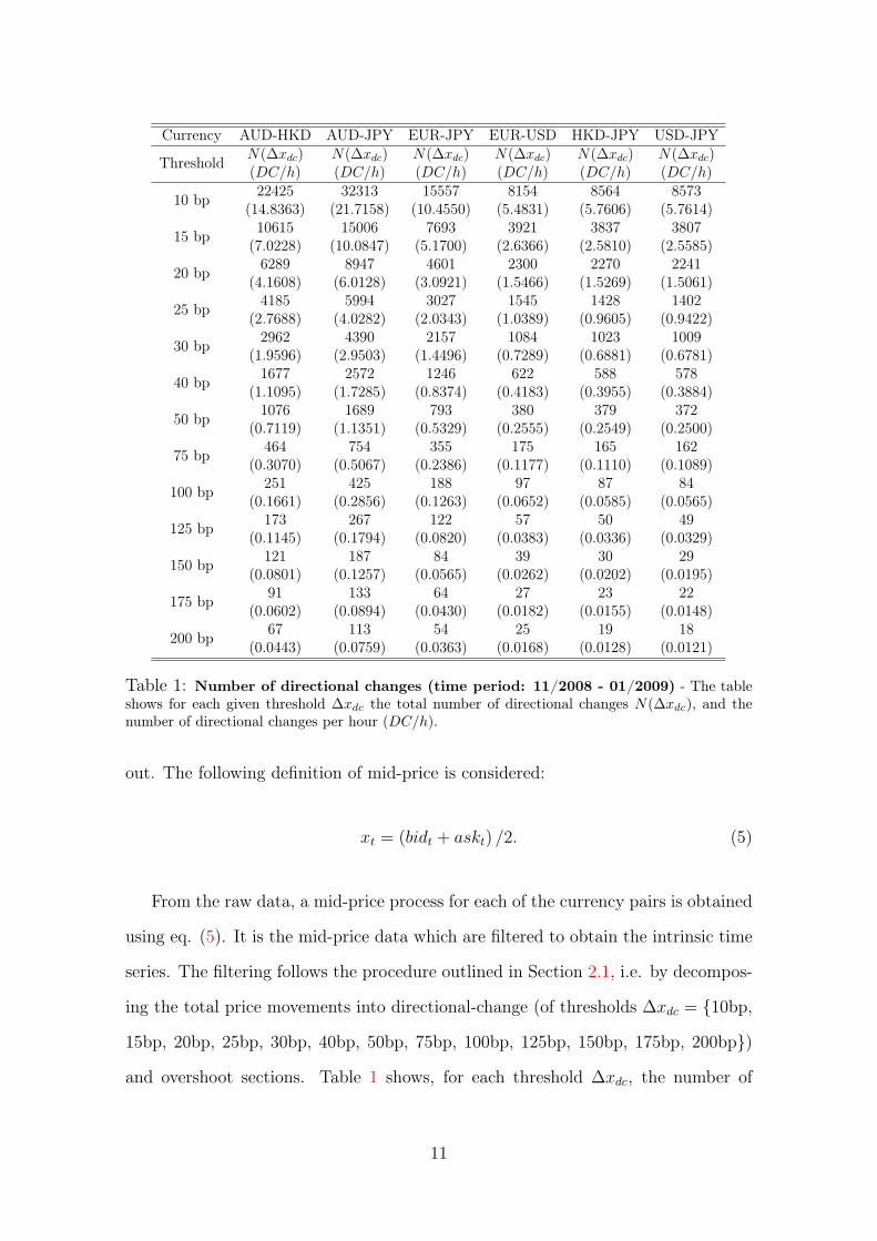
Table 1: Number of directional changes (time period: 11/2008 - 01/2009) - The tableshows for each given threshold ∆xdc the total number of directional changes N(∆xdc), and thenumber of directional changes per hour (DC/h).

out. The following definition of mid-price is considered:

xt = (bidt + askt) /2. (5)

From the raw data, a mid-price process for each of the currency pairs is obtained

using eq. (5). It is the mid-price data which are filtered to obtain the intrinsic time

series. The filtering follows the procedure outlined in Section 2.1, i.e. by decompos-

ing the total price movements into directional-change (of thresholds ∆xdc = {10bp,

15bp, 20bp, 25bp, 30bp, 40bp, 50bp, 75bp, 100bp, 125bp, 150bp, 175bp, 200bp})

and overshoot sections. Table 1 shows, for each threshold ∆xdc, the number of

11

Figure 2: Empirical scaling law: estimated scaling law regression lines for the different currencypairs (time period: 11/2008 - 01/2009). The x-axis shows the threshold size as relative pricechange, and the y-axis the respective average time (in seconds), for a given threshold, to observethe reversion of the price move.

directional changes N(∆xdc) and the “speed” of change of the mid-price process,

measured in directional changes per hour (DC/h).

Figure 2 illustrates the power law regression (eq. 2) for the currency pairs consid-

ered in this paper. Table 2 lists the intercept, slope, associated R2 and mean square

error (MSE) statistics. For each of the currency pairs, we also show the results for

a geometric Brownian motion (GBM), which we used as a benchmark. Given an

initial mid-price x0, the process generated is

xt = x0 · e(µ−σ2

2

)t+σWt , (6)

where xt ∼ GBM(µ, σ2), Wt is a Wiener process, and µ and σ are estimated from

the data. The regression coefficients for the GBM are obtained by averaging the

12

Currency Intercept SlopeR2 MSE(s.e.) (s.e.)

AUD-HKD 8.1806 1.9407 0.9996 2.7E-4(0.0258) (0.0111)

GBM 5.9829 1.7176 0.9965 0.0021(0.0704) (0.0304)

AUD-JPY 7.8952 1.8985 0.9995 3.3E-4(0.0284) (0.0123)

GBM 5.6690 1.6578 0.9952 0.0027(0.0802) (0.0346)

EUR-JPY 8.2895 1.9316 0.9994 4.8E-4(0.0342) (0.0148)

GBM 6.1383 1.7451 0.9970 0.0019(0.0667) (0.0288)

EUR-USD 8.7042 1.9768 0.9990 8.2E-4(0.0445) (0.0192)

GBM 6.5774 1.8115 0.9978 0.0015(0.0578) (0.0249)

HKD-JPY 8.9131 2.0520 0.9982 0.0015(0.602) (0.0260)

GBM 6.5938 1.8149 0.9978 0.0015(0.0585) (0.0252)

USD-JPY 8.9539 2.0656 0.9983 0.0015(0.0604) (0.0260)

GBM 6.6002 1.8158 0.9978 0.0015(0.0585) (0.0252)

Table 2: Empirical scaling law - Estimated regression parameters (time period: 11/2008- 01/2009). The scaling law relates the average time interval for directional changes of giventhresholds to occur to the size of the thresholds. For each currency pair, the last two rows showthe regression parameters and the corresponding standard errors of the benchmark geometricBrownian motion (GBM).

OLS estimates over a sufficiently high number of iterations, so as to ensure good

convergence properties. The slope of the curves (the key parameter in the power-

law) are close to those reported in Glattfelder, Dupuis, and Olsen (2011), with

similar associated statistics. This similarity illustrates the remarkable robustness of

the scaling law as the data used in this investigation are later than those employed

by Glattfelder, Dupuis, and Olsen (2011). In particular, it is noted that all the

currency pairs show power-law behaviour which is statistically different from the

corresponding GBM at the 99% confidence level.

Following the data filtering, the dissection (cut-off) points between directional-

change and overshoot sections generate a new irregularly-spaced time series of

13

directional-change events in intrinsic time; the LSFT is then applied to calculate the

SDF. Since the LSFT relies on the assumption of weak-stationarity of the data, the

DC mid-price series were detrended, taking into account the irregularity in spacing

between two contiguous observations, and tested for stationarity prior to the esti-

mation of the spectral density. The Augmented Dickey-Fuller (Dickey and Fuller,

1981) and Phillips-Perron (Phillips and Perron, 1988) unit root tests were applied

to assess the stationarity of the data at different lags, assuming an autoregressive

model for the (detrended) mid-price process.

Figures 3A, 3B, and 3C show examples of the SDFs of mid-price directional-

change events (in the top panels) and the corresponding false-alarm probabilities

(in the bottom panels) of the currency pair EUR-JPY for 3 different thresholds

(0.5%, 0.75%, 1.5%). For a better comparison with the corresponding results for

the remaining currency pairs (see Appendix), the spectral densities are normalised

by the maximum of SDFLS. 3A illustrates that all the significant peaks (for a

significance level of 95%) are located in the left-hand side of the graph2, i.e. that the

highest contribution to the variance of the mid-price process comes from relatively

low frequencies (corresponding to a period longer than 23 hours). On the other hand,

Figures 3B and 3C illustrate that, as the directional-change threshold increases, the

spectral density tends to shift further towards the left-hand side of the graph, that is

towards the lower frequencies. All the significant peaks correspond in fact to periods

longer than 138 and 824 hours, respectively for thresholds of 0.75% and 1.5%. This

is perfectly consistent with the expectation that, as the directional-change threshold

increases, the time needed to trigger that threshold also increases.

In particular, the scaling property of directional-change durations assures that

in the frequency domain, periodicities associated with a particular threshold are

replicated in the empirical spectral densities of directional-change events of those

of lower thresholds. Table 3 (∆xdc = {10bp, 15bp, 20bp}) and Table 4 (∆xdc =

2 The frequency axis was truncated below the median value, thereby excluding frequencies forwhich the spectral density was substantially lower than the significance level.

14

(A) EUR-JPY

(B) EUR-JPY

(C) EUR-JPY

Figure 3: Empirical spectral density of directional-change events and associatedfalse alarm probabilities for EUR-JPY rate. The upper panels show the empiricalspectral densities (normalised) of mid-price directional change events for the thresholds0.50% (3A), 0.75% (3B) and 1.5% (3C), respectively. The lower panel shows the corre-sponding false alarm probabilities of the estimated spectral density at 95% s.l. for a givenfrequency expressed in Hz. The associated period in hours is indicated in the secondaryx-axis.

15

Threshold AUD-HKD AUD-JPY EUR-JPY EUR-USD HKD-JPY USD-JPY20 bp 11.8697 11.8443 7.9351 10.2617 8.2999

7.9392 11.3039 8.3098 6.17117.9278 7.8178 6.0028

6.9007 4.77716.29406.00154.77613.91403.4909

15 bp 11.8731 11.8445 11.8380 11.8587 8.2992 10.246111.3385 11.3041 7.9341 7.3817 8.29997.9414 10.9100 6.7989 6.0271

7.9385 6.02667.8133 4.81545.96384.77203.9170

10 bp 11.8732 11.8446 11.8650 11.8589 10.0204 10.022611.3173 11.3042 10.3022 7.9323 9.2556 9.272110.4739 10.9301 7.9364 8.3107 8.312510.0724 7.9386 7.4772 6.9014 6.91099.6695 7.8134 5.9622 6.0326 6.02789.3119 7.4698 4.7746 5.9067 4.81648.7207 5.9639 4.0192 5.1137 4.61457.9415 5.5622 4.8153 3.27107.8283 4.7721 4.6134 3.16487.4888 4.6635 3.27217.1690 3.9170 3.16586.4636 2.67245.97185.07854.78124.09453.91923.13622.80962.1116

Table 3: Scaling property of directional-change durations for the currency pairs (timeperiod: 11/2008 - 01/2009) - The table lists for the three thresholds ∆xdc = {10bp, 15bp, 20bp}a subsample of periods below 12 hours with significant peaks of the estimated spectral density at> 95% confidence level.

{25bp, 50bp, 75bp}) report for the selected thresholds the corresponding periods

expressed in hours, associated with significant peaks of the estimated spectral density

at the 99% significance level. It can be seen that the periodicities associated with

the 150bp threshold (see 3C) are replicated in the spectral density of directional-

16

Threshold AUD-HKD AUD-JPY EUR-JPY EUR-USD HKD-JPY USD-JPY75 bp 333.6198 328.9597 197.4176 168.1769 202.4595

261.0938 197.3758200.1719 123.3599171.5759 80.017223.4576

50bp 335.4352 330.3823 197.9385 236.5594 203.8477 203.6614251.5764 247.7868 179.2117 120.6445 120.5343194.7688 198.2294 72.9158

123.893480.363363.2647

25 bp 335.6498 330.3083 197.9252 246.7681 282.6001 282.5144251.7374 247.7312 80.2399 185.0761 197.8200 197.7601194.8934 198.1850 63.1676 24.4729 72.3732 73.2445125.8687 123.8656 25.7046 25.3615 24.515781.6445 80.3453 23.3770 21.3475 21.341061.0272 42.4682 20.9815 16.039542.2496 35.3902 11.8518 10.249737.7606 28.7225 4.778328.6336 25.8502 3.490925.8192 23.407724.5597 21.310223.4174 18.522021.0512 17.642611.8697 13.095911.314 11.8437

7.9380

Table 4: Scaling property of directional-change durations for the currency pairs (timeperiod: 11/2008 - 01/2009) - The table lists for the three thresholds ∆xdc = {25bp, 50bp, 75bp}a subsample of periods below 336 hours (2 weeks) with significant peaks of the estimated spectraldensity at > 95% confidence level.

change events sampled with both the 75bp and 50bp thresholds (see 3B and 3C).

Similarly, the additional periodicities associated with the 75bp threshold are again

propagated in the 50bp threshold and so on. If we observe a 150bp price change

about every 360 hours on average (see Table 3), for example, we should also observe

a 75bp and a 50bp price change at each full cycle.3 In other words, for the same

frequency in the spectral density of a directional change series sampled with a higher

threshold, one can also find a corresponding significant peak in the spectral density3Differences in the values might occur as “rounding errors” as the periods are actually calculated

as reciprocal values from the original frequencies that are expressed in Hz. As discernible in Table3, the lower the reported period (i.e., the higher the estimated frequency), the smaller are the gapsbetween the values across the different thresholds.

17

sampled with a lower threshold - despite the irregular spacing in (physical) time.

This remarkable behaviour in the frequency domain is due to the scaling properties

in the time domain, and is evident for other thresholds for the EUR-JPY FX rate,

as well as for the other currency pairs investigated in this study. This finding is not

to be confused with the aliasing or masking effect in standard spectral analysis as we

consider the time series in event time (all irregularly spaced in time and differently

sampled depending on the threshold).

In general, similar conclusions can be drawn analysing a different currency pair.

For example, the spectral density of the AUD-HKD mid-price (see Figure 5) exhibits

periodicities similar to those of the corresponding SDF of the currency pair EUR-

JPY, showing an analogous trend, as the period associated with the directional

changes tends to get longer as the directional-change threshold increases. Results

for the other FX pairs with similar implications are shown in the Appendix (see

Figures 5 to 8).

Future research will focus on the application of the proposed approach in algo-

rithmic trading: for example, once a significant periodic component with period τ

has been detected for a given price p0, a simple trading strategy could be devised

whereby the agent takes a short or a long position on the asset held, if its cur-

rent market price is, respectively, above or below the target price p0, and closes the

positions after time τ , or when the asset price reaches again the initial level p0.

4 Conclusion

Ultra-high frequency (UHF) data are observed in real-time and therefore are char-

acterised by the irregularity of time intervals between two consecutive events. This

paper combines the Lomb-Scargle Fourier Transform (LSFT) and an event-based

approach, to analyse foreign exchange tick-by-tick data. The LSFT implicitly takes

into account the non-periodic property of UHF data without the need to first trans-

18

form the data to a periodic array. Using empirical transaction data from FX markets

and adopting an event-based time scale (known as intrinsic time), the spectral anal-

ysis shows that various parts of the whole price process display different periodic

patterns, revealed by the energy of the process in the respective frequency domain.

The period associated with these patterns tends to increase as the directional-change

threshold increases, confirming similar results in other studies (see e.g. Glattfelder,

Dupuis, and Olsen, 2011).

Interestingly, the scaling property of directional-change durations in the time

domain, has also notable repercussions in the frequency domain. In fact, if a price

series is irregularly spaced in time, it can be filtered using a given DC threshold

contains periodic components, which then can be detected in series filtered at lower

thresholds. For the same frequency in the spectral density of a DC series sampled

with a high threshold, one can also detect a corresponding peak, above the signifi-

cance level, in the spectral density of prices sampled using a lower threshold. The

same analysis extended to stochastic overshoots, exhibit a similar behaviour, thus

implying the existence of equivalent periodic patterns in the frequency domain.

Further, by using a set of different directional-change thresholds, this event-

setting allows us not only to model the behaviour of market agents with different risk

preferences and dealing frequencies, but also to capture seasonal volatility patterns

present in the data.

References

Aldridge, I. (2010): High-Frequency Trading: A Practical Guide to Algorithmic

Strategies and Trading Systems. Wiley, 1 edn.

Bauwens, L., W. Ben Omrane, and P. Giot (2005): Journal of International

Money and Finance24(7), 1108–1125.

19

Ben Omrane, W., and E. de Bodt (2007): “Using self-organizing maps to adjust

for intra-day seasonality,” Journal of Banking & Finance, 31(6), 1817–1838.

Bisig, T., A. Dupuis, V. Impagliazzo, and R. B. Olsen (2012): “The scale of

market quakes,” Quantitative Finance, 12(4), 501–508.

Bouchaud, J.-P. (2001): “Power laws in economics and finance: some ideas from

physics,” Quantitative Finance, 1(1), 105–112.

Bouchaud, J.-P. (2002): “An introduction to statistical finance,” Physica A: Sta-

tistical Mechanics and its Applications, 313(1-2), 238–251.

Bretthorst, G. L. (2001): “Generalizing the Lomb-Scargle periodogram-the non-

sinusoidal case,” in Bayesian Inference and Maximum Entropy Methods in Science

and Engineering, vol. 568, pp. 246–251.

Chordia, T., R. Roll, and A. Subrahmanyam (2001): “Market Liquidity and

Trading Activity,” The Journal of Finance, 56(2), 501–530.

Dacorogna, M. M., R. Gençay, U. A. Müller, R. B. Olsen, and O. V.

Pictet (2001): An Introduction to High-Frequency Finance. Academic Press, 1

edn.

Derman, E. (2002): “The perception of time, risk and return during periods of

speculation,” Quantitative Finance, 2(4), 282–296.

deVilliers, V. (1933): The Point and Figure Method of Anticipating Stock Prices:

Complete Theory & Practice. Windsor Books.

Dickey, D. A., and W. A. Fuller (1981): “Likelihood Ratio Statistics for Au-

toregressive Time Series with a Unit Root,” Econometrica, 49(4), 1057–72.

Giampaoli, I., W. L. Ng, and N. Constantinou (2009): “Analysis of ultra-high-

frequency financial data using advanced Fourier transforms,” Finance Research

Letters, 6(1), 47–53.

20

Glattfelder, J. B., A. Dupuis, and R. B. Olsen (2011): “Patterns in high-

frequency FX data: discovery of 12 empirical scaling laws,” Quantitative Finance,

11(4), 599–614.

Guillaume, D. M., M. M. Dacorogna, R. R. Davé, U. A. Müller, R. B.

Olsen, and O. V. Pictet (1997): “From the bird’s eye to the microscope: A

survey of new stylized facts of the intra-daily foreign exchange markets,” Finance

and Stochastics, 1(2), 95–129.

Hautsch, N. (2004): Modelling Irregularly Spaced Financial Data. Springer, Hei-

delberg.

Horne, J. H., and S. L. Baliunas (1986): “A prescription for period analysis of

unevenly sampled time series,” Astrophysical Journal, 302, 757–763.

Lomb, N. R. (1976): “Least-squares frequency analysis of unequally spaced data,”

Astrophysics and Space Science, 39, 447–462.

Lyons, R. K. (2001): The Microstructure Approach to Exchange Rates. MIT Press,

Cambridge, Mass.

MacDonald, R. (2007): Exchange Rate Economics: Theories and Evidence. Rout-

ledge, London.

Mandelbrot, B., and H. M. Taylor (1967): “On the distribution of stock prices

differences,” Operations Research, 15(6), 1057–1062.

Phillips, P. C. B., and P. Perron (1988): “Testing for a unit root in time series

regression,” Biometrika, 75(2), 335–346.

Press, W. H., B. P. Flannery, S. A. Teukolsky, and W. T. Vetterling

(1992): Numerical Recipes in C: The Art of Scientific Computing. Cambridge

University Press, 2 edn.

21

Press, W. H., and G. B. Rybicki (1989): “Fast algorithm for spectral analysis

of unevenly sampled data,” Astrophysical Journal, 338, 277–280.

Priestley, M. B. (1981): Spectral Analysis and Time Series. Volume 1: Univari-

ate Series. Academic Press, 1st edn.

Scargle, J. D. (1982): “Studies in astronomical time series analysis. II - Statistical

aspects of spectral analysis of unevenly spaced data,” Astrophysical Journal, 263,

835–853.

Van Dongen, H., E. Olofsen, J. Van Hartevelt, and E. Kruyt (1999):

“A Procedure of Multiple Period Searching in Unequally Spaced Time-Series with

the Lomb-Scargle Method,” Biological Rhythm Research, 30, 149–177.

Ware, A. F. (1998): “Fast Approximate Fourier Transforms for Irregularly Spaced

Data,” SIAM Review, 40, 838–856.

Wyckoff, R. D. (1910): Studies in tape reading. The Ticker Publishing Company,

New York.

Appendix

22

(A) EUR-USD

(B) EUR-USD

(C) EUR-USD

Figure 4: Empirical spectral density of directional-change events and associatedfalse alarm probabilities for EUR-USD rate. The upper panels show the empiricalspectral densities (normalised) of mid-price directional change events for the thresholds0.50% (4A), 0.75% (4B) and 1.5% (4C), respectively. The lower panel shows the corre-sponding false alarm probabilities of the estimated spectral density at 95% s.l. for a givenfrequency expressed in Hz. The associated period in hours is indicated in the secondaryx-axis.

23

(A) Threshold = 0.50%

(B) Threshold = 0.75%

(C) Threshold = 1.5%

Figure 5: Empirical spectral density of directional-change events and associatedfalse alarm probabilities for AUD-HKD rate. The upper panels show the empiricalspectral densities (normalised) of mid-price directional change events for the thresholds0.50% (??), 0.75% (5B) and 1.5% (5C), respectively. The lower panel shows the corre-sponding false alarm probabilities of the estimated spectral density at 95% s.l. for a givenfrequency expressed in Hz. The associated period in hours is indicated in the secondaryx-axis.

24

(A) Threshold = 0.50%

(B) Threshold = 0.75%

(C) Threshold = 1.5%

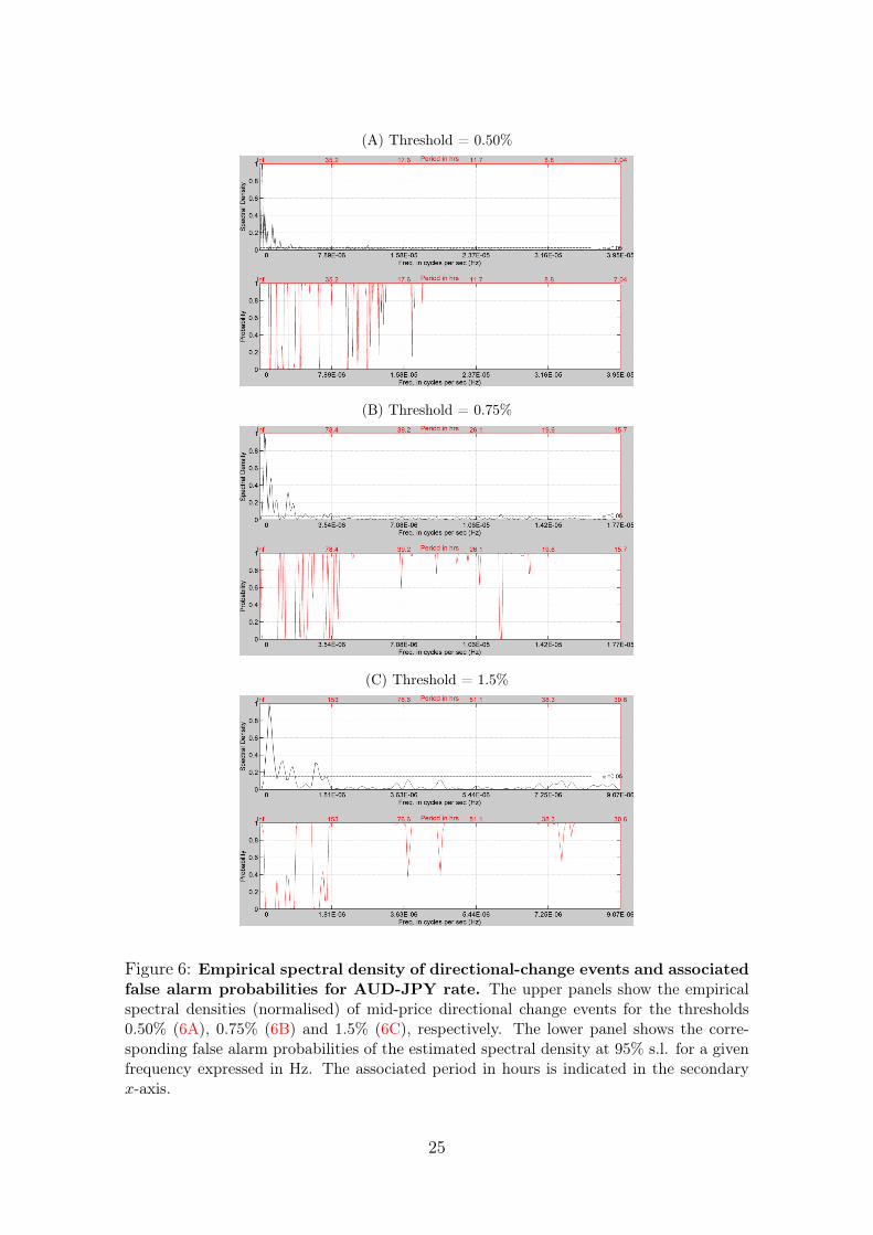
Figure 6: Empirical spectral density of directional-change events and associatedfalse alarm probabilities for AUD-JPY rate. The upper panels show the empiricalspectral densities (normalised) of mid-price directional change events for the thresholds0.50% (6A), 0.75% (6B) and 1.5% (6C), respectively. The lower panel shows the corre-sponding false alarm probabilities of the estimated spectral density at 95% s.l. for a givenfrequency expressed in Hz. The associated period in hours is indicated in the secondaryx-axis.

25

(A) Threshold = 0.50%

(B) Threshold = 0.75%

(C) Threshold = 1.5%

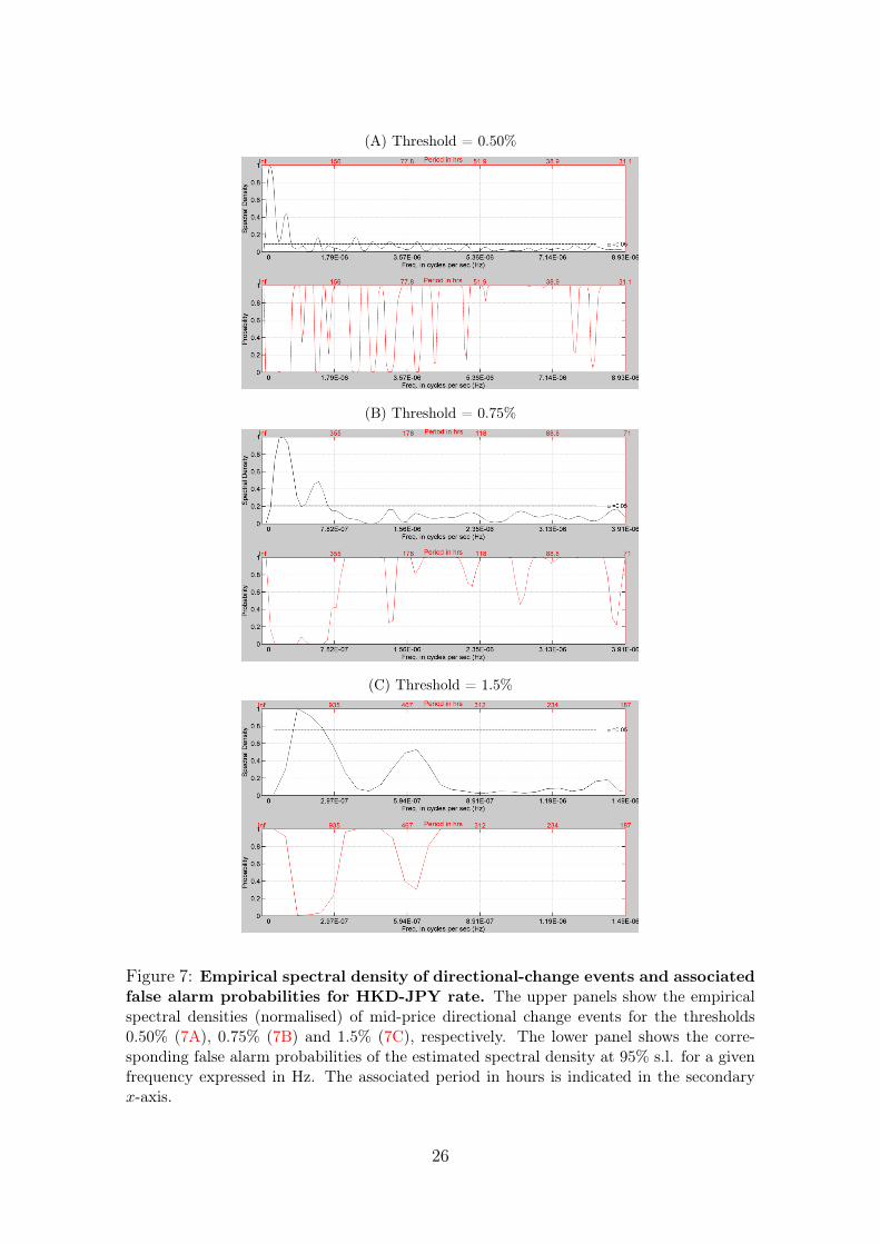
Figure 7: Empirical spectral density of directional-change events and associatedfalse alarm probabilities for HKD-JPY rate. The upper panels show the empiricalspectral densities (normalised) of mid-price directional change events for the thresholds0.50% (7A), 0.75% (7B) and 1.5% (7C), respectively. The lower panel shows the corre-sponding false alarm probabilities of the estimated spectral density at 95% s.l. for a givenfrequency expressed in Hz. The associated period in hours is indicated in the secondaryx-axis.

26

(A) Threshold = 0.50%

(B) Threshold = 0.75%

(C) Threshold = 1.5%

Figure 8: Empirical spectral density of directional-change events and associatedfalse alarm probabilities for USD-JPY rate. The upper panels show the empiricalspectral densities (normalised) of mid-price directional change events for the thresholds0.50% (8A), 0.75% (8B) and 1.5% (8C), respectively. The lower panel shows the corre-sponding false alarm probabilities of the estimated spectral density at 95% s.l. for a givenfrequency expressed in Hz. The associated period in hours is indicated in the secondaryx-axis.

27