WP/20/ - elibrary.imf.org

WP/20/91

Government Spending Effects in a Policy Constrained Environment

by Ruoyun Mao and Shu-Chun Susan Yang

©International Monetary Fund. Not for Redistribution

© 2020 International Monetary Fund WP/20/91

IMF Working Paper

Fiscal Affairs Department

Government Spending Effects in a Policy Constrained Environment

Prepared by Ruoyun Mao and Shu-Chun S. Yang

Authorized for distribution by Catherine Pattillo

June 2020

Abstract The theoretical literature generally finds that government spending multipliers are bigger than unity in a low interest rate environment. Using a fully nonlinear New Keynesian model, we show that such big multipliers can decrease when 1) an initial debt-to-GDP ratio is higher, 2) tax burden is higher, 3) debt maturity is longer, and 4) monetary policy is more responsive to inflation. When monetary and fiscal policy regimes can switch, policy uncertainty also reduces spending multipliers. In particular, when higher inflation induces a rising probability to switch to a regime in which monetary policy actively controls inflation and fiscal policy raises future taxes to stabilize government debt, the multipliers can fall much below unity, especially with an initial high debt ratio. Our findings help reconcile the mixed empirical evidence on government spending effects with low interest rates.

JEL Classification Numbers: E32, E52, E62, E63, H30

Keywords: government spending effects, fiscal multiplier, regime-switching policy, monetary and fiscal policy interaction, nonlinear New Keynesian models

Authors’ E-Mail Address: [email protected]; [email protected]

________________________

*Mao: Department of Economics, Indiana University; Yang: Fiscal Affairs Department, International MonetaryFund. We thank Philip Barrett, Jean-Berard Chatelain, Christopher Erceg, Vitor Gaspar, Eric Leeper, SimingLiu, Marialuz Moreno Badia, Adrian Paralta Alva, Catherine Pattillo, Babacar Sarr, David Savitski, HeweiShen, Todd Walker, and participants of the seminar at the Fiscal Affairs Department of the IMF, 2019 MidwestMacro Meetings, and the UCA-CNRS-IRD-CERDI International Workshop on Policy Mix for helpfulcomments and discussion.

1

IMF Working Papers describe research in progress by the author(s) and are published to elicit comments and to encourage debate. The views expressed in IMF Working Papers are those of the author(s) and do not necessarily represent the views of the IMF, its Executive Board, or IMF management.


mailto:[email protected]

mailto:[email protected]

Contents

1 I ntr o ducti on 3

2 The M o de l Se tup 7

2 . 1 Ho us eho l ds . . . . . . . . . . . . . . . . . . . . . . . . . . . . . . . . . . . . . . . 7

2 . 2 F i r m s . . . . . . . . . . . . . . . . . . . . . . . . . . . . . . . . . . . . . . . . . . 82 . 3 T he P ubl i c Sect o r . . . . . . . . . . . . . . . . . . . . . . . . . . . . . . . . . . . 9

2 . 3 . 1 F i s ca l Po l i cy . . . . . . . . . . . . . . . . . . . . . . . . . . . . . . . . . . 1 02 . 3 . 2 M o net a r y Po l i cy . . . . . . . . . . . . . . . . . . . . . . . . . . . . . . . . 1 0

2 . 4 Funct i o na l Fo r m s , Pa r a m et er i za t i o n, a nd t he So l ut i o n M et ho d . . . . . . . . . . 1 1

3 Gove r nm e nt Sp e ndi ng Effe cts : Re gi m e F v s . Re gi m e M 13

3 . 1 Si mul a t i o ns w i t h t he Ba s el i ne C a l i br a t i o n . . . . . . . . . . . . . . . . . . . . . . 1 43 . 2 A Hi g her St o ck o f Ini t i a l G over nm ent D ebt . . . . . . . . . . . . . . . . . . . . . 1 6

3 . 3 A Hi g her Level o f Ta xa t i o n . . . . . . . . . . . . . . . . . . . . . . . . . . . . . . 1 83 . 4 A Lo ng er D ebt M a t ur i ty w i t h a M o r e Res p o ns i ve M o net a r y Po l i cy . . . . . . . . 2 0

4 Pol i cy Re gi m e Unce r tai nty 22

4 . 1 Po l i cy Reg i m e Uncer t a i nty i n Reg i m e F . . . . . . . . . . . . . . . . . . . . . . . 2 34 . 2 Po l i cy Reg i m e Uncer t a i nty i n Reg i m e M . . . . . . . . . . . . . . . . . . . . . . . 2 4

5 Gove r nm e nt Sp e ndi ng Effe cts i n Re ce s s i ons 25

5 . 1 M a cr o eco no m i c D yna m i cs i n Reces s i o ns : Reg i m e M vs . Reg i m e F . . . . . . . . 2 6

5 . 2 F i s ca l M ul t i pl i er s i n Reces s i o ns w i t h t he Bi ndi ng Z LB . . . . . . . . . . . . . . . 2 7

6 Se ns i ti v i ty A nal y s i s 29

6 . 1 No m i na l pr i ce r i g i di ty . . . . . . . . . . . . . . . . . . . . . . . . . . . . . . . . . 2 9

6 . 2 Per s i s t ence i n G over nm ent Sp endi ng Incr ea s es . . . . . . . . . . . . . . . . . . . . 3 06 . 3 G over nm ent D ebt i n t he St ea dy St a t e . . . . . . . . . . . . . . . . . . . . . . . . 3 1

6 . 4 T he La b o r Inco m e Ta x Ra t e i n t he St ea dy St a t e . . . . . . . . . . . . . . . . . . 3 2

7 C oncl us i on 33

A pp e ndi ce s 39

A Eq ui l i br i um Sy s te m 39

B De te r m i ni s ti c Ste ady State 40

C C om putati onal A l gor i thm 41

2


Underline

1 Introduction

More than a decade after the global financial crisis in 2007-2008, most advanced economies

have not returned to their pre-crisis macroeconomic policies. Government debt in advanced

economies remains elevated, averaging 105 percent of GDP in 2019, compared to 72 percent in

2007 (International Monetary Fund (2019a)). Meanwhile, monetary policy in most advanced

economies has been loose and accommodative. The constrained policy environment is illustrated

in Figure 1. Economies like the euro area and Japan are trapped at the effective zero lower bound

(ZLB), and the U.S. reversed the course on interest rate normalization as signs of weakness

emerged since 2019 (International Monetary Fund (2019b)), and the federal funds rate hit the

ZLB again in March 2020 as the coronavirus outbreak has posed a severe risk to the U.S. and

the global economy.

2002 2004 2006 2008 2010 2012 2014 2016 20180

2

4

% p

er

annum

the euro area

60

70

80

90

% o

f G

DP

main refinancing rate

public debt

2002 2004 2006 2008 2010 2012 2014 2016 20180

2

4

% p

er

annum

Japan

140

170

200

230%

of

GD

P

call rate

public debt

2002 2004 2006 2008 2010 2012 2014 2016 20180

2

4

% p

er

annum

United States

50

70

90

110

% o

f G

DPfederal funds rate

public debt

Figure 1: Constrained policy environment. The annual policy rates are monthly averages. Thepolicy rate of the European Central Bank is the main refinancing rate of the ECB Key Interest Rates.The policy rate of Japan is the Call Money/Interbank Rate. Public debt is the gross public debt ofgeneral governments from the database of the World Economic Outlook (International Monetary Fund(2019a)).

3


With high government debt and low interest rates, should the government pursue expan-

sionary fiscal policy to counteract economic downturns? The theoretical literature (e.g., Kim

(2003), Davig and Leeper (2011), and Christiano et al. (2011)) generally predicts that gov-

ernment spending multiplier is much bigger than one when monetary policy does not actively

respond to inflation or is at the ZLB. Among the few empirical studies available, the evidence,

however, is divided on supporting more expansionary government spending effects with low in-

terest rates. Miyamoto et al. (2018) estimate that in Japan, the impact output multiplier is

0.6 in the normal period (1980Q1-1995Q3) and 1.5 in the ZLB period (1995Q4-2014Q1). Also,

Jacobson et al. (2019) estimate that the peak output multipliers of fiscal expansions are 3.6-4.5

during the 1933-1940 recovery period in the U.S. when the gold standard was abandoned. On

the other hand, Almunia et al. (2010), Ramey (2011), and Ramey and Zubairy (2018) do not

find clear support that government spending multipliers are bigger when interest rates are low.

To reconcile with the mixed empirical evidence, this paper studies the factors that can

dampen the expansionary effects of government spending under passive monetary policy. Specif-

ically, we focus on nonlinear government spending effects in policy regime F, in which monetary

policy is passive and fiscal policy is active in Leeper’s (1991) terminology. The results are com-

pared to government spending effects in the commonly analyzed regime M—active monetary

policy and passive fiscal policy—in the literature (e.g., Forni et al. (2009), Cogan et al. (2010),

and Traum and Yang (2015)). Confirming the findings in Leeper et al. (2017) with a linearized

model, we also find that higher steady-state distorting labor income taxation and longer debt

maturity decrease government spending multipliers in regime F. Using a fully nonlinear solution,

we bring new insights on the role of initial government debt levels and policy regime uncertainty

in affecting government spending effects in regime F.

We first compare government spending effects under the two fixed regimes: regime F vs.

regime M.1 In regime M, the monetary authority stabilizes inflation and the fiscal authority

raises taxes. In regime F, by contrast, the fiscal authority does not raise taxes (sufficiently) to

debt increases and the monetary authority does not actively respond to inflation. Different from

regime M, where government debt is stabilized through fiscal backing (raising taxes as modeled

1In Bianchi and Melosi (2017, 2019), they refer to regime M as a monetary-led regime and regime F as afiscal-led regime.

4


here), government debt in regime F is stabilized mainly through inflation. Consistent with Kim

(2003), Davig and Leeper (2011), and Dupor and Li (2015), multipliers in regime F are generally

bigger than one and those in regime M. Both the intertemporal substitution effect and wealth

effect channels contribute to the very different multipliers. In regime F, weak responses in the

nominal interest rate plus rising inflation from more government spending lower the real interest

rate, reversing the crowding-out effect in regime M. Moreover, lack of fiscal backing in regime F

eliminates the negative wealth effects of government spending that crowds out private demand

in regime M.

The very expansionary government spending effects in regime F, however, can diminish by

various factors, particularly relevant for advanced economies. The first one is high debt burden.

Since government debt is stabilized through inflation, a higher initial debt stock provides a

bigger “tax base” for “inflation taxes,” and hence inflation increases by less to stabilize debt.

A smaller inflation increase leads to a smaller decline in the real interest rate, weakening the

intertemporal substitution effect that crowds in consumption.

Other factors include higher tax burden (modeled by a higher steady-state labor income tax

rate), longer average debt maturity, and more responsive monetary policy to inflation. All these

factors work through the intertemporal substitution effect channel. Although the government

does not increase the tax rate in response to more debt in regime F, part of the additional debt

is financed by increased tax revenues because of an enlarged tax base. Thus, with a higher

steady-state tax rate, a bigger proportion of a spending increase is financed by taxes, so the

debt amount to be inflated away is smaller. As the inflation rate does not increase as much,

the intertemporal substitution effect is weakened. Similarly, longer debt maturity implies that

the required inflation adjustment can be spread over a longer horizon. When combined with a

bigger response of the nominal interest rate to inflation (monetary policy remaining passive),

the output multiplier can fall below one. Although a smaller inflation increase erodes the bond

income by less, the overall consumption response can turn negative because of the rising real

interest rate.

Next, we allow for regime switching to study how policy uncertainty can affect government

spending effects and interact with other factors. Following Davig and Leeper (2011), we assume

that the two policy regimes switch according to a two-state Markov chain. Instead of constant

5


transition probabilities, we deviate from their setting by assuming that the switching probability

from regime F to M is state-dependent and time-varying: households in regime F place a higher

switching probability to regime M upon observing higher inflation. In regime F, expectations

of switching to regime M lower expected inflation, leading current inflation to increase by less

relative to the case without such expectations. Lower expected inflation then produces a smaller

crowding-in effect. Also, expectations of switching to regime M imply rising expected future

taxes, invoking negative wealth effects. This offsets some positive consumption responses from

a negative real interest rate in regime F. When combining policy uncertainty with high initial

debt, the output multipliers can fall substantially below one. Since high levels of inflation are

uncommon in advanced economies in last three decades, inflation-dependent policy uncertainty

in regime F can be empirically relevant.

In addition to regime F, policy uncertainty also has negative effects on output multipliers

in regime M, although the negative impact is relatively small. In regime M, expectations of

switching to regime F increase expected inflation and hence current inflation more relative to

the case without such expectations. Since the Taylor rule still operates, the monetary author-

ity raises the nominal interest rate more, exacerbating the crowding-out effects of government

spending and produces smaller output multipliers in regime M relative to the case without pol-

icy uncertainty. The crowding-out effect, however, is somewhat offset by diminished negative

wealth effects, because policy uncertainty makes households place some probability that future

tax rates do not increase once switching to regime F.

Aside from government spending effects in normal times, we also examine them in recessions.

We inject sufficiently negative structural shocks such that the economy is driven to a deep

recession with the binding ZLB. Although several papers have studied theoretical government

spending effects in recessions, they tend to focus on the ZLB in regime M (e.g., Michaillat

(2014) and Canzoneri et al. (2016)). Unlike the typical results that a recession or the ZLB can

generate much bigger output multipliers (e.g., Christiano et al. (2011), Woodford (2011), and

Erceg and Linde (2014)), we find that a recession or the ZLB may not enhance government

spending effects in regime F. In regime M, government spending at the ZLB generates higher

inflation and reduces the real interest rate, producing a much bigger multiplier than in normal

times—similar to the intertemporal substitution effect channel making the multiplier bigger in

6


regime F than in M. In regime F, on the other hand, high inflation from a government spending

increase makes the economy immediately exit the ZLB. Unless the monetary authority becomes

less responsive to inflation (e.g., pegging the net interest rate at zero), the initial ZLB does not

enhance government spending effects in recessions.

Our analysis of government spending effects in regimes F and M is closely related to two

recent papers that compare the conventional debt-financed and money-financed government

spending effects. English et al. (2017) and Galı (forthcoming) find that a money-financed gov-

ernment spending increase crowds in private consumption and is more expansionary than a

debt-financed one. The main mechanisms underlying these results are the same as those driving

bigger multipliers in regime F.2 This implies that the factors we highlight which can weaken the

expansionary effects of government spending in regime F are likely to be relevant for money-

financed government spending effects.

2 The Model Setup

We adopt a New Keynesian (NK) model with nominal price rigidity as modeled in Rotemberg

(1982).3 The key features deviating from a standard NK model include: 1) flexible government

debt maturities, a la Woodford (2001)4 and 2) the possibility of switching between regimes F

and M.

2.1 Households

The representative household chooses consumption (ct), labor (nt), and nominal government

bonds (Bt) for each period t to maximize the lifetime utility by solving the following optimization

problem:

maxE0

∞∑

t=0

βtU(ct, nt), (2.1)

2Beck-Friis and Willems (2017) analytically show that in regime F with lump-sum taxes, government spendingfinanced by nominal debt is equivalent to money-financed spending.

3We choose Rotemberg’s (1982) mechanism instead of Calvo’s (1983) to reduce the number of state variablesrequired in solving the model nonlinearly.

4Traum and Yang (2011) show that when only a short-term debt is included, regime F requires an unusuallyhigh degree of price stickiness to reconcile inflation dynamics in data and in an NK model.

7


subject to

ct +QtBt − (1− κ)Bt−1

Pt=Bt−1

Pt+ (1 − τt)wtnt + Υt + zt + ξt, (2.2)

where ct ≡[

∫ 10 ct(i)

θ−1θ di

]θ

θ−1is a basket of goods aggregated by the Dixit-Stiglitz aggregator,

Pt is the price of the composite good, wt is the real wage rate, and τt is the labor income

tax rate. The left hand side of (2.2) is the total expenditure, including consumption and the

purchase of (net) newly issued government bond. The right hand side is households’ income,

consisting of income from savings—bond payment from the government, after-tax labor income,

dividends from owning the firms (Υt), government transfers (zt), and the rebate of nominal price

adjustment costs (ξt) to be explained in firms’ problem.

Following Woodford (2001), we assume that households have access to a portfolio of govern-

ment bonds, Bt, which sells at a price of Qt at t and pays (1 − κ)t dollars t + 1 periods later

for each t ≥ 0. The average bond maturity is (1 − β(1 − κ))−1 quarters. The usual setting of

short-term government bonds is nested with κ = 1. The transversality condition for bond is

limT→∞

Et {qt,TDT} = 0, (2.3)

where qt,T =RT−1

(PT /Pt)and DT ≡ BT−1 [1 + (1 − κ)QT ].

2.2 Firms

The production sector consists of a continuum of monotonically competitive firms. Each

firm i chooses price (Pt(i)) and labor (nt(i)) to maximize the present value of future nominal

profits, discounted by the household’s stochastic discounting factor:

maxnt(i),Pt(i)

Et

∞∑

s=0

βsλt+s

λt

[

Pt+s(i)yt+s(i)−Wt+snt+s(i)−ψ

2

(

Pt+s(i)

π∗Pt+s−1(i)− 1

)2

yt+sPt+s

]

, (2.4)

subject to linear technology for each intermediate good i:

yt(i) = Ant(i), (2.5)

8


and the demand for each intermediate good i:

yt(i) =

(

Pt(i)

Pt

)−θ

yt, (2.6)

where yt ≡[

∫ 10 yt(i)

θ−1θ di

]θ

θ−1is the final goods, π∗ is the inflation target set by the monetary

authority, and A is technology assumed to be constant. The discounting factor between time t+s

and t follows from the household’s Euler equation, βs λt+s

λt, with λt = Uct , the marginal utility of

consumption. Price adjustments are subject to a quadratic adjustment cost with an adjustment

parameter ψ > 0 to govern nominal price rigidity. In aggregation, the price adjustment cost,

ξt ≡ψ2 ( πt

π∗ − 1)2yt, is rebated back to households, as shown in (2.2).5

To solve for the optimality condition, rewrite (2.4) in real terms:

maxnt(i),Pt(i)

Et

∞∑

s=0

βt+sλt+s

λt

[(

Pt+s(i)

Pt+s

)1−θ

yt+s−wt+snt+s(i)−ψ

2

(

Pt+s(i)

π∗Pt+s−1(i)−1

)2

yt+s

]

. (2.7)

Solving firms’ optimization problem and imposing the symmetric equilibrium conditions yield

the Phillips curve:

ψ

(

πt

π∗− 1

)

πt

π∗= (1− θ) + θmct + βψEt

[

λt+1

λt

yt+1

yt

πt+1

π∗

(

πt+1

π∗− 1

)]

, (2.8)

where πt ≡Pt

Pt−1is gross inflation and mct ≡

wt

A it the real marginal cost.

2.3 The Public Sector

The public sector consists of a fiscal authority and a monetary authority. The two policy

regimes analyzed are defined in terms of different responses of fiscal adjustment to government

indebtedness and monetary policy to inflation.

5As shown in Eggertsson and Singh (2019) and Miao and Ngo (forthcoming), when the adjustment costis rebated back to households, the results under Calvo (1983) and Rotemberg (1982) are closer when inflationchanges are large than without the rebate. This is relevant for our analysis government spending in regime Ftends to generate a big jump in inflation.

9


2.3.1 Fiscal Policy

Each period the government collects a proportional labor income tax and issues nominal

bonds to finance its goods purchases (gt) and transfers to households (zt), subject to the following

flow budget constraint:

QtBt − (1 − κ)Bt−1

Pt+ τtwtnt =

Bt−1

Pt+ gt + zt. (2.9)

Since our focus is on expansionary fiscal policy through goods purchases, we assume that gov-

ernment purchases follow an exogenous AR(1) process:

lngt

g= ρg ln

gt−1

g+ ε

gt , (2.10)

where the innovation εgt ∼ i.i.d.N(

0, σ2g

)

and g is steady-state government goods purchases. For

simplicity, we assume that transfers are constant at the steady-state level: zt = z.

The labor income tax rate responds to debt and the coefficient, γ(st), is regime-dependent:

τt = τ + γ(st)(bt−1 − b) ·R

R− (1− κ), γ(st) ∈ {γF , γM}, (2.11)

where bt ≡Bt

Ptis real government debt, b and R are the steady-state real debt and nominal

interest rate, st indicates the state of the policy regime (F or M), and γM > γF ≥ 0. With

long-term debt, government indebtedness is captured by the the face value of outstanding debt—

defined as the sum of the present value of all future payments, discounted by the steady-state

nominal interest rate.6

2.3.2 Monetary Policy

The monetary authority determines the short-term nominal bond return based on a non-

linear response to inflation deviation from the inflation target, π∗:

Rt = max

{

1, R ·( πt

π∗

)α(st)}

, α(st) ∈ {αF , αM}, (2.12)

6At the steady state, the face value of government bonds is the same as the market value.

10


where α(st) is the regime-dependent response to inflation deviation. When the unconstrained

interest rate rule implies a gross nominal interest rate below 1, the economy is at the ZLB,

Rt = 1.

We follow Leeper (1991) and Leeper et al. (2017) to define regime M, in which the monetary

authority actively controls inflation and the fiscal authority raises taxes to stabilize debt, and

regime F, in which the monetary authority does not stabilize inflation and the fiscal authority

does not stabilize debt. We initially assume that the economy has fixed policy regimes. When

studying policy uncertainty, the fixed regime assumption is relaxed in Section 4.

2.4 Functional Forms, Parameterization, and the Solution Method

We assume the representative household’s utility function is:

U(ct, nt) =(ct − νt)

1−σ

1 − σ− χ

n1+ϕt

1 + ϕ. (2.13)

where νt affects consumption taste as in Erceg and Linde (2014) and Battistini et al. (2019).

While most analysis does not involve shocking νt, we inject negative taste shocks to generate a

recession when analyzing government spending effects in such a state. The taste shock follows

a stationary AR(1) process:

νt = ρννt−1 + ενt , (2.14)

where νt ∼ i.i.d.N(

0, σ2ν

)

.

Since our model setup is mostly a standard NK model, we adopt common values for the

structural parameters of the baseline calibration. Table 2.4 summarizes the parameter and policy

values in the steady state. We calibrate the model at a quarterly frequency. The discounting

factor, β, is set to 0.992, implying an annualized real interest rate around 3%. The quarterly

inflation target is set to 1.005, matching the annualized 2% inflation target adopted in most

advanced economies. The risk aversion parameter in the utility function is set to σ = 2. The

labor disutility parameter, χ, is endogenously calculated to produce a steady-state labor of

n = 0.25. The steady-state technology is set to A = 1, equivalent to having a normalized

steady-state yearly output of 1. The inverse Frisch elasticity is set to ϕ = 2, to be consistent

11


with the values from estimated NK models.7 We follow Davig and Leeper (2011) to set θ = 7.66.

This implies a 15% of price markup in the steady state. The Rotemberg quadratic cost parameter

is set to ψ = 78, implying the degree of nominal price rigidity to be about one year (as estimated

in Smets and Wouters (2007) for the probability that firms can choose prices optimally).8

The baseline calibration sets κ = 1 to have the common setting of only short-term debt,

so it can be compared to an alternative case of longer debt maturity—κ = 0.05. This implies

the average debt maturity of about 20 quarters, matching the average maturity of total U.S.

outstanding Treasury marketable debt from 2000 to 2018 of about five years (Office of Debt

Management (2018)). We adopt other fiscal values in the steady states to follow Drautzburg

and Uhlig (2015) with U.S. data. The steady-state debt-to-annual output ratio is 0.6, and the

government goods purchase-to-output ratio is 0.15. The steady-state labor income tax rate is

set to τ = 0.28, and transfers are endogenously computed to satisfy the government budget

constraint in the steady state.

To calibrate γ(st) and α(st) in the tax and interest rate policy rules, (2.11) and (2.12), we

set the values consistent with Leeper’s (1991) definitions for active/passive monetary and fiscal

policies:{

st = F: α(st) = αF , γ(st) = γF ;

st = M: α(st) = αM , γ(st) = γM .(2.15)

To reflect the typical slow process of debt adjustment in reality, γM is set to the smallest value

that meets the transversality condition for government debt, (2.3).9

For exogenous processes, we set the process of the taste shock to be ρν = 0.8 and σν = 0.0025.

This process determines how often the economy hits and remains at the ZLB. Our calibration

implies that the conditional probability of hitting the ZLB is about 5% in regime M, typical

of NK models subject to the ZLB (e.g., see Miao and Ngo (forthcoming) for 5.6% in an NK

7For instance, the posterior estimate is 1.96 in Smets and Wouters (2007) and 2.16 in Drautzburg and Uhlig(2015). In Leeper et al. (2017), the estimated value is 1.77 in regime M and 2.34 in regime F.

8Under first-order approximation and a zero net inflation target, Rotemberg (1982) is equivalent to Calvo(1983), and ψ = (θ−1) ω

(1−ω)(1−ωβ), where ω is the fraction of the firms that cannot reset prices in Calvo’s setting.

Since the model here is fully nonlinear and the net inflation target is not zero, we cannot back up a precise ψ tomatch a certain price adjustment frequency in Calvo (1983). The sensitivity analysis explores the role of nominalprice rigidity in output multipliers under different policy regimes.

9Since we cannot solve the model analytically, the precise parameter ranges that distinguish regimes M andF cannot be obtained. The policy functions show that debt is stabilized differently across the two regimes. Inparticular, government debt is an important state in regime F but not so in regime M.

12


Parameters Values Source and Target

Structural parameters

discounting factor (β) 0.992 annualized real interest rate of 3%

risk aversion (σ) 2

inverse of Frisch elasticity (ϕ) 2

elasticity of substitution (θ) 7.66 15% price markup at the steady state

price adjustment cost (ψ) 78 implied price rigidity: one year

government debt maturity (κ) 1 short-term debt

Policy parameter or steady-state values

targeted inflation (π∗) 1.005 annualized inflation target 2%

steady state debt to GDP ratio ( b4y ) 0.6 Drautzburg and Uhlig (2015)

steady state government spending to GDP ratio ( gy ) 0.15 Drautzburg and Uhlig (2015)

steady state labor tax rate (τ) 0.28 Drautzburg and Uhlig (2015)

interest rate response to inflation in regime M (αM) 1.5 Bianchi and Melosi (2017)

tax rate response to debt in regime M (γM) 0.15 Bianchi and Melosi (2017)

interest rate response to inflation in regime F (αF ) 0.5 Bianchi and Melosi (2017)

tax rate response to debt in regime F (γF ) 0 by definition

Exogenous processes

persistence of taste (ρν) 0.8 probability of hitting ZLB: 5% as in

standard deviation of the taste shock (σν) 0.0025 Miao and Ngo (forthcoming)

persistence of government purchase (ρg) 0.9 Shen and Yang (2018)

standard deviation of government purchase (σg) 0.01 Shen and Yang (2018)

Table 1: Baseline Calibration

model).10 The economy has a government spending persistence of ρg = 0.9 with a standard

deviation of 0.01, based on Shen and Yang’s (2018) estimate. Sensitivity analysis explores

different government spending persistence.

The model is solved fully non-linearly with Euler equation iteration, following Coleman

(1991) and Davig (2004). Appendix A contains the equilibrium system, Appendix B calculates

the deterministic steady state, and Appendix C describes the solution method.

3 Government Spending Effects: Regime F vs. Regime M

We begin our analysis by explaining the channels that drive the different government spend-

ing effects in the two regimes and identify relevant factors that diminish the expansionary effects

of government spending in regime F in a fixed regime environment.

10The persistent parameter, ρν , is set to 0.85 in Battistini et al. (2019) and 0.9 in Erceg and Linde (2014). Wechoose a slightly lower persistence ρν = 0.8; otherwise, it would imply a much higher probability of hitting theZLB in the simulations allowing for switching to regime F.

13


0 20 40 600

0.5

1

%

G/Y

0 20 40 60-0.5

0

0.5

%

consumption

0 20 40 60

0

0.5

1

1.5

%

output

0 20 40 600

1

2

3

4

%

real wage

0 20 40 600

1

2

3

4

%

nominal debt

0 20 40 600

1

2

3

4

%

tax revenue

0 20 40 6028

28.1

28.2

28.3

%

tax rate

0 20 40 6058

59

60

61

62

%

debt-to-GDP

0 20 40 60

0

0.5

1

%

inflation

0 20 40 60

0

0.2

0.4

0.6

%

nominal rate

0 20 40 60-0.3

-0.2

-0.1

0

0.1

%

real rate

Regime M

Regime F

Figure 2: Simulations with the baseline calibration: regime F vs. regime M. Impulse responsesto a government spending increase. Except for G/Y (the government spending-to-steady state outputratio), inflation, nominal rate, real interest rate, and expected inflation, the y-axis units are in percentdeviation from a path without a government spending shock. For G/Y, the graph plots level differencesin percent. For inflation, the nominal rate, the real interest rate, and expected inflation, the graphs plotannualized level differences. The x-axis unit is in quarters after the government spending shock.

3.1 Simulations with the Baseline Calibration

Figure 2 compares the effects of an initial government spending increase of 1% of steady-

state output in the two regimes with the parameters in Table 2.4. Unless specified in the figure

notes, the plots show the differences between the paths with and without a spending shock

in percentage deviations from the latter path.11 In fully non-linear models, the size of the

government spending shock and the initial state of the economy both matter for government

spending effects. Thus, for all experiments we fix the size of the government spending increase

at one percent of the steady-state output and fix the initial debt level at its deterministic steady

state—60% of the annualized steady-state output, unless specified otherwise.

Consistent with the literature (Kim (2003), Davig and Leeper (2011), Dupor and Li (2015),

11To calculate one-year ahead inflation expectations, we simulate the impulse response sequences 10,000 timesfor both paths with and without a government spending increase, by drawing from the taste shock distributioneach period. The one-year ahead inflation expectation at time t is the average of the inflation differences at t+ 4between the two paths in each simulation. Although our calculation is the ex-post average of inflation, underrational expectations, the average inflation for t+4 (based on 10,000 simulations) should be very close to Et(πt+4).

14


and Dupor et al. (2018)), government spending in regime F is more expansionary and generates

much higher inflation than in regime M. Two main forces driving the very different responses

are via the wealth-effect channel and the intertemporal substitution effect channel. Households

in regime M expect higher future tax burden, which discourages consumption and encourages

saving, producing an output multiplier smaller than one. In regime F, this negative wealth effect

does not operate because the future tax rate is not expected to rise in response to higher debt.

The real wage rate rises because the stimulus increases firms’ labor demand, and more wage

income supports higher consumption.12 On the intertemporal substitution effect, the monetary

authority in regime M raises the nominal interest rate more than the inflation increase (αM > 1),

hence an increase in the real interest rate. Instead, the monetary authority in regime F does not

raise the nominal interest rate sufficiently to control inflation so the the real interest rate falls,

reversing the typical crowding-out effect of government spending in regime M. Also, in regime F,

the strong demand increases together with muted interest rate responses generate much higher

inflation (4.2% in regime F vs. 0.5% in regime M on impact), as shown in Figure 2.

Table 2 summarizes the cumulative output multipliers in present value under different cali-

brations, computed as∑k

j=0

(

∏ji=0 rt+i

−1)

∆yt+j∑k

j=0

(

∏ji=0 rt+i

−1)

∆gt+j, (3.1)

where ∆y and ∆g are level changes relative to the paths without a government spending increase

and rt ≡Rt

Et(πt+1) is the gross real interest rate. When j = 0,∏ji=0 rt+i

−1 ≡ 1. Under the baseline

calibration, the impact output multiplier is 1.27 in regime F, compared to 0.58 in regime M,

and the differences remain large for longer horizons (0.90 in regime F vs. 0.45 in regime M five

years after). Although consumption multipliers are not reported, its impact multiplier is 0.27 in

regime F under the baseline calibration, compared to −0.42 in regime M, reflecting crowding-in

vs. crowding-out effects in the two regime.13

The rest of this section explores each of the factors in Table 2 that can reduce the expan-

12Note that in regime M, the wage rate also increases but by a much smaller magnitude than that in regimeF. A higher wage rate (together with higher labor) also increases labor income in regime M, but households saveadditional income for future taxes.

13In our closed-economy model without investment, yt = ct + gt; the consumption multiplier is equal to theoutput multiplier minus one. Our analysis does not account for the possibility in an open-economy environmentthat capital inflows can help finance a fiscal expansion (such as aid), which can mitigate the crowding-in effectsof a government spending increase. See Broner et al. (2018) and Shen et al. (2018).

15


sionary effect of government spending in regime F.

regime M regime F

impact 4Q 20Q impact 4Q 20Q

baseline 0.58 0.56 0.45 1.27 1.15 0.90

high government debt ( b04y = 1) 0.58 0.56 0.44 1.19 1.08 0.85

high income tax rate (τ = 0.5) 0.58 0.56 0.43 1.07 0.98 0.80

long-term debt (κ = 0.05) 0.59 0.57 0.49 1.11 1.01 0.81

long-term debt & more responsive MP (κ = 0.05, αF = 0.8) - - - 0.89 0.86 0.78

Table 2: Cumulative output multipliers: fixed policy regimes. The multipliers are calculated asdescribed in (3.1). b0

4ydenotes the initial debt-to-annual output when the government spending takes

place. The baseline case has b0

4y= 0.6, τ = 0.28, αF = 0.5, and κ = 1. For other cases, we hold all the

parameters the same as the baseline values except for the one specified in parentheses.

3.2 A Higher Stock of Initial Government Debt

A major concern associated with increasing government spending is elevated government

debt in many advanced economies after the global financial crisis. Several empirical studies

show that government spending is less expansionary in a high-debt state than in a low-debt

state (e.g., Kirchner et al. (2010), Ilzetzki et al. (2013), and Nickel and Tudyka (2014)). One

plausible explanation is that high debt may induce expectations of larger fiscal adjustment (Bi

et al. (2016)). This mechanism cannot operate in regime F though, as the government does not

raise tax rates or implement other fiscal adjustment measures to stabilize debt. By solving the

model fully nonlinearly, we can explore the role of initial government indebtedness on government

spending effects in regime F.14 We find that a high initial debt level also reduces the government

multiplier in regime F, but the underlying mechanism is quite different from expecting bigger

fiscal adjustments in regime M.

To examine debt dependence of government spending effects in regime F, we simulate gov-

ernment spending effects when an initial debt ratio is 100%. The first two rows in Table 2 show

that the output multipliers are smaller across various horizons in regime F when an initial debt

ratio is higher: the impact output multiplier is 1.19 with 100% of initial debt, compared to 1.27

14Most papers that study government spending effects in regime F solve for a log-linearized equilibrium aroundthe steady state, and the analysis is typically conducted from the steady-state debt level. We carry out thisexperiment in Section 6.

16


0 2 4 6 8 10-0.2

0

0.2

0.4

%

consumption

0 2 4 6 8 10-1.8

-1.6

-1.4

-1.2

-1

-0.8

%

household bond income

0 2 4 6 8 100

1

2

3

4

5

%

inflation

0 2 4 6 8 10

-1

-0.8

-0.6

-0.4

-0.2

0

%

real rate

initial debt = 60%

initial debt = 100%

Figure 3: The role of government indebtedness in government spending effects in regime F.The axis units and the government spending path follow those in Figure 2.

with 60% of initial debt.15

Figure 3 compares the impulse responses for these two simulations. It shows that in regime

F, an initial debt of 100% leads to a smaller increase in inflation and hence a smaller decline in

the real interest rate than the case of 60%. For a given government spending increase, higher

government debt provides a bigger base for inflation taxes; consequently, the inflation rate need

not increase as much as with a smaller stock of debt. Lower inflation implies that the real

interest rate does not fall as much, which generates a smaller intertemporal substitution effect

15In our simulation, the initial debt level has almost no influence on multipliers in regime M. This is differentfrom the finding in Bi et al. (2016), where the baseline economy assumes a GHH (Greenwood et al. (1988))preference and no negative wealth effect on labor. We use a constant-relative-risk-aversion utility instead. Also,their income taxes include capital income taxes and we only have labor income taxes here. With a high initialdebt level, expecting higher capital income tax rates discourages current investment and offsets some of theexpansionary effect of government spending.

17


and hence a smaller increase in consumption, leading to the smaller output multipliers.

Note that rising inflation in regime F also reduces the real value of households’ holding of

government bonds. As the top-right plot in Figure 3 shows, households’ real bond income,

calculated as bt−1

πt, decreases in both cases because of higher inflation.16 With 100% of initial

debt, inflation increases less and therefore the drop in household’s real bond income is smaller

than the case of 60%. Despite a smaller reduction in bond income, consumption increases less

with the 100% debt level, as the intertemporal substitution effect channel dominates the negative

bond income effect on consumption.

The two opposite forces arising from higher initial debt in affecting consumption in regime F

imply that the overall effect is relatively small. Later when we incorporate the factor of policy

regime uncertainty, the intertemporal substitution effect channel gets amplified substantially,

and government spending multipliers can drop much below one with a marginal increase in the

initial debt ratio from 0.6 to 0.7.

Our closed-economy model assumes that government debt is held only by domestic house-

holds. If a large proportion of debt is held abroad (such as the case of the U.S.), the role of

government indebtedness in driving the difference in the multipliers in regime F would be more

pronounced. In the extreme case with all government debt held by foreigners, consumption

would increase more with the initial debt ratio of 60% than 100%, because the avoided negative

consumption effect from declined bond income is bigger with the former case.

3.3 A Higher Level of Taxation

Next, we explore the role of tax burden on government spending effects in regime F, a factor

particularly relevant for the European countries. We compare the baseline economy (τ = 0.28)

to two different levels of the steady-state distorting labor tax rate: τ = 0 and τ = 0.5. Figure 4

shows that a higher steady-state tax rate leads to a smaller increase in inflation and, hence, a

smaller decrease in the real interest rate than with a lower tax rate.

In regime F, the economy with a higher steady-state tax rate implies that a bigger proportion

of a government spending increase is financed by tax revenues from output expansion, despite

16The simulation here assumes only short-term debt (κ = 1), so the nominal value of savings income from

bond holding at t isBt−1

Pt.

18


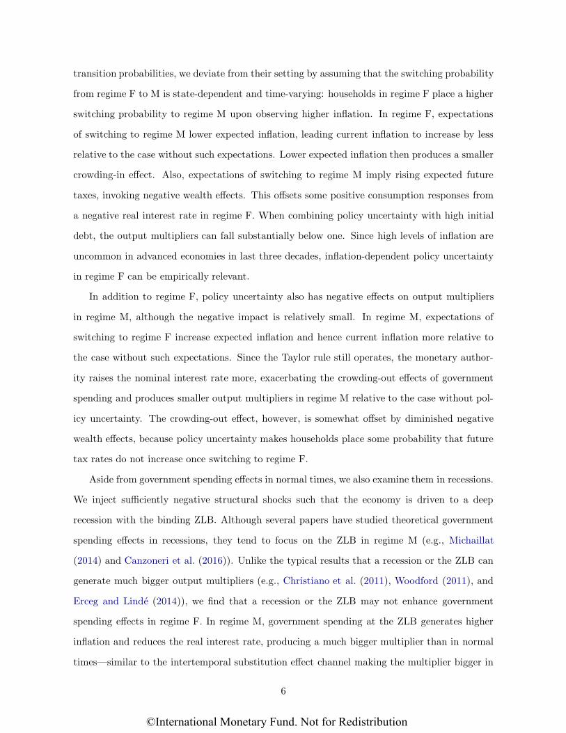
that the government does not raise the tax rate to finance debt (γF = 0). For a given government

spending increase, this means that inflation does not increase as much and the real interest rate

does not decrease as much, weakening the intertemporal substitution effect channel. As shown

in Figure 4, consumption and the real wage rate rise the most with τ = 0. A strong increase in

goods demand from consumption implies strong labor demand, driving the largest increase in

the real wage rate with τ = 0. While the change in the labor income tax rate in response to a

spending increase in regime F is zero across the three cases (γF = 0), labor responses are quite

different because of different crowding-in effects, as shown in Figure 4.

0 5 10

0

0.2

0.4

0.6

0.8

1

%

consumption

0 5 100

0.5

1

1.5

2

%

output

0 5 100

2

4

6

%

wage

0 5 100

2

4

6

8

10

%

inflation

0 5 10

-2

-1.5

-1

-0.5

0

%

real rate

= 0

= 0.28

= 0.5

Figure 4: The role of the steady-state labor income tax rate in regime F. The increase ofgovernment spending follows the path in Figure 2. See Figure 2 for axis units.

Table 2 shows that a higher steady-state tax rate decreases the output multipliers in regime

F, but has little effect in regime M. For a given government spending increase in regime M, it

must be financed by a certain amount of debt and future taxes. In the economy with a low

steady-state tax rate, for a given size of a government spending increase, the amount of debt

that needs to be issued at time zero is bigger than in the case with a high steady-state tax

19


rate. While the negative wealth effect is bigger with a low steady-state tax rate (because the

government issues more debt), a lower current tax burden implies a bigger increase in the after-

tax income. By the same reasoning, a higher steady-state tax rate has a smaller negative wealth

effect and a smaller increase in the after-tax income. In either case, the combined effect (from

the negative wealth effect and positive income effect) is about the same on current consumption,

and thus produces very similar output multipliers with different steady-state tax rates. This

result is consistent with the finding of Leeper et al. (2017) in a linearized model.

3.4 A Longer Debt Maturity with a More Responsive Monetary Policy

From Figure 3, we see that inflation and inflation expectations to a government spending

increase in regime F rise much more than in regime M. The typical short-term debt specification

overstates the inflation responses and, hence, the crowding-in effect of government spending.

Consistent with Leeper et al. (2017), we find that longer average debt maturity lowers the

consumption and output multipliers in regime F. Table 2 shows that the impact output multiplier

with an average maturity of approximately five years is 1.11, compared to the baseline short-term

debt multiplier of 1.27.17 With only short-term debt, the government must repay a relatively

large amount of liabilities next period, requiring an immediate inflation adjustment to stabilize

debt, whereas longer-term debt permits inflation to be spread to future periods. As the left plot

of Figure 5 shows, longer average debt maturity lowers current and near future inflation (the

dotted line), leading to smaller multipliers than those with only short-term debt.

Another relevant factor that also reduces short-run inflation responses in regime F is the

response of monetary policy to inflation. Although monetary policy in regime F does not actively

respond to inflation, the responsiveness still shapes the paths of current inflation and inflation

expectations. As the right plot of Figure 5 shows, with an average maturity of five years, a bigger

response of the nominal interest rate (a bigger αF in (2.12) but still in Regime F) limits the

increase in inflation in the short run and pushes inflation to the future. As the initial inflation

rises less, again it leads to a smaller decline in the real interest rate and hence smaller output

and consumption multipliers.

17The average maturity of total U.S. outstanding Treasury marketable debt from 2000 to 2018 is five years(Office of Debt Management (2018)).

20


0 2 4 6 8 100

0.5

1

1.5

2

2.5

3

3.5

4

4.5%

inflation

= 1

= 0.05

0 2 4 6 8 10-0.5

0

0.5

1

1.5

2

2.5

3

3.5

4

%

inflation

F = 0.2

F = 0.5

F = 0.8

Figure 5: The role of debt maturity and monetary policy’s response to inflation in regime

F. The left panel compares inflation responses to a government spending increase under short-term debt(κ = 1) and long-term debt (κ = 0.05). The right panel compares inflation responses to a governmentspending increase under different monetary policy responses, conditional on an average debt maturity ofabout five years (κ = 0.05). The increase of government spending follows the path in Figure 2.

The last row of Table 2 presents the multipliers for an average five-year debt maturity

(κ = 0.05) combined with a more responsive interest rate policy (α = 0.8). While still in regime

F, output multipliers throughout the horizon drop below one and the consumption multipliers

turn negative as in regime M. On impact, the output multiplier falls to 0.89 with five-year average

debt maturity. Since the average government debt maturity in reality is much longer than one

quarter, and the monetary authority may not refrain from responding to inflation completely,

the combination of the two factors suggest that government spending multipliers can easily fall

below one in regime F.

The analysis in this section focuses on the factors that can diminish the expansionary effects

of government spending under passive monetary policy. Our cashless model cannot simulate the

effects of a money-financed government increase. The results obtained here, however, are likely

to be relevant for the expansionary effects of money-financed government spending in English

21


et al. (2017) and Galı (forthcoming), because the main mechanisms underlying its big multipliers

are similar to those in regime F.

4 Policy Regime Uncertainty

In the above fixed regime environment, households believe that the current regime will

never change and there is no policy regime uncertainty. Over the past thirty years, central

banks in advanced economies have been emphasizing their independence and many of them

have announced inflation targets. With this historical experience, mounting inflation generated

by government spending in regime F is likely to induce households to expect a switching to

regime M. To see how this expectation can affect government spending effects, we follow Davig

and Leeper (2006, 2007, 2011) to assume that the policymakers’ behavior is captured by a

two-state Markov chain with the transition matrix below:

st+1 = M st+1 = F

st = M ρMM 1− ρMM

st = F 1 − ρFF ρFF

(4.1)

where st indicates the state of the policy regime. Deviating from their assumption of constant

regime switching probabilities, we assume that households’ expectations about switching back to

regime M depend on observed last-period inflation. Specifically, we assume that the transition

probability from regime F to M is an increasing function of last-period inflation in the following

logistic form:

ρFF =

1, if πt−1 ≤ π∗;

exp(

Φ(πt−1))

1+exp(

Φ(πt−1)) otherwise,

(4.2)

where Φ(πt−1) = α1(πt−1/π∗−1) governs how much the probability of staying in regime F decreases

as inflation rises. To mimic the inflation-targeting policy in reality, we assume that households

do not expect policy to switch to regime M until inflation rises above the targeted level, π∗.

Figure 6 plots the probability of staying in regime F as a function of last-period inflation (πt−1)

under different values of α1. To make the model tractable, we assume that ρMM is constant

22


over time. Specifically, for the simulation below, we set α1 = 0.05 and fix ρMM = 0.98, which

implies an average duration of 50 quarters in regime M.18

0.98 1 1.02 1.04 1.06 1.08 1.1

t-1

0.5

0.6

0.7

0.8

0.9

1F

F1 = 0.01

1 = 0.03

1 = 0.05

Figure 6: Regime switching probability: ρFF . The y-axis is the probability in regime F at t to stayat regime F at t+ 1. See equation (4.2) for the functional form that links ρFF to last-period inflation.

4.1 Policy Regime Uncertainty in Regime F

To see how regime switching expectations affect government spending multipliers in regime

F, we simulate a scenario with an initial debt-to-annual output ratio at 70%.19 Relative to

the baseline multiplier (Table 2), Table 3 shows that output multipliers are much smaller when

households expect that future policy can switch to regime M. Also, the higher the initial debt

ratio is, the higher the probability households place on switching, and the smaller are the output

multipliers. The impact output multiplier with a debt ratio of 80% decreases to 0.76, compared

to 1.27 in the baseline without policy regime uncertainty.

In regime F, when households expect that the monetary authority can switch back to ac-

18We also experiment with ρMM from 0.95-0.99, and its value does not affect the results as long as regime Mis sufficiently persistent.

19The deterministic steady-state debt ratio of 0.6 is lower than the stochastic steady-state ratio defined bythe mean of the ergodic distribution. Therefore, the corresponding inflation is below the target even with agovernment spending increase of 1% of steady-state output. Since we assume that the probability of switchingto regime M is zero unless inflation of last period exceeds the targeted inflation rate, we need a higher initialgovernment debt to induce households to place a positive regime switching probability.

23


impact 4Q 20Q

baseline (fixed regime F) 1.27 1.15 0.90

initial debt-to-annual output: 0.7 0.90 0.87 0.86

initial debt-to-annual output: 0.8 0.76 0.74 0.78

Table 3: Cumulative output multiplier in regime F with expectations of switching to regime

M. The multipliers are calculated as described in (3.1).

tively controlling inflation, it lowers inflation expectations, and hence, current inflation. Lower

expected inflation drives up the current real interest rate, induces households to consume less,

and thus lowers current goods demand relative to the case without such expectations. Moreover,

with some probability of switching to regime M, households expect that future tax rates may

increase and start saving for a potential tax hike, even though they are still in regime F.

Section 3 shows that government indebtedness seems to only have small quantitative effects

in reducing government spending multipliers, as the impact multiplier with an initial debt ratio

of 100% in regime F only drops to 1.19 from 1.27 with a ratio of 60% (see Table 2). With regime

switching possibility, the analysis shows that policy uncertainty can substantially amplify the

negative effect of high debt burden in lowering government spending multipliers in regime F.

The above simulations with regime switching policies are conducted in an economy with

short-term debt (κ = 1). We also repeat the simulations in an economy with an average debt

maturity of about five years (κ = 0.05). The magnitude of multiplier reductions relative to a

fixed regime F with longer debt maturity is similar to those in Table 3.

4.2 Policy Regime Uncertainty in Regime M

Given that policy uncertainty can significantly lower multipliers in regime F, a natural ques-

tion to ask whether it plays a similar role in regime M. Different from the state-dependent

switching probabilities, we assume the switching probability from regime M to F is constant.

Table 4 compares the output multipliers under different switching probabilities of ρMM .

As the probability of switching to regime F increases, output multipliers also become smaller

relative to the baseline case without uncertainty, but the difference is not as big as in regime F.

In regime M, while the monetary authority actively raises the nominal interest rate in response

to inflation, the expectation that government debt can be inflated away drives up expected

24


inflation and, hence, current inflation.20 Since the current policy remains in regime M, higher

inflation induces a bigger response in the nominal interest rate, aggravating the crowding-out

effect of government spending in regime M. Meanwhile, expecting a switch to regime F reduces

the expected future tax rates. This works to increase government spending multipliers relative

to the case without such expectation. Thus, the overall effect of policy uncertainty in regime M

is generally small because the negative effect from expecting higher inflation is offset to some

extent by the positive effect from expecting lower future taxes.

impact 4Q 20Q

fixed regime (ρMM = 1) 0.58 0.56 0.45

middle switching probability (ρMM = 0.98) 0.53 0.50 0.29

high switching probability (ρMM = 0.95) 0.46 0.39 -0.08

Table 4: Cumulative output multiplier in regime M with expectations of switching to regime

F. The multipliers are calculated as described in (3.1). The initial debt-to-annual output is 0.6.

5 Government Spending Effects in Recessions

Theoretical literature studying business cycle state-dependent multipliers at the binding

ZLB mainly focuses on regime M (e.g., Christiano et al. (2011), Michaillat (2014), Canzoneri

et al. (2016), and Shen and Yang (2018)), and not much is known about government spending

effects in recessions with regime F. In this section, we study how government spending effects

differ in recessions under the two policy regimes. We consider a recession that the ZLB can

bind for a sustained period in regime M with a series of negative taste shocks, following the

common practice in the literature (e.g., Eggertsson and Woodford (2003, 2006), Christiano et al.

(2011), Erceg and Linde (2014), Fernandez-Villaverde et al. (2015)). Since the economy responds

to the same macroeconomic shocks quite differently in the two regimes, we first compare the

macroeconomic responses before analyzing government spending effects.

20Bianchi and Melosi (2017) use this mechanism to explain why there was no deflationary spiral in the 2008recession as predicted by standard NK models.

25


5.1 Macroeconomic Dynamics in Recessions: Regime M vs. Regime F

In non-linear models, initial states can affect economic responses to shocks. Thus, we design

simulations such that the two economies begin with the same state—both in regime M at t = 0—

and are hit by the same negative taste shocks from t = 1 to t = 5. At t = 3, one economy stays

in regime M and the other switches to regime F, with the policy parameters in Table 2.4.

0 10 20-2

-1.5

-1

-0.5

0

%

taste shock

0 10 20-8

-6

-4

-2

0

%

consumption

0 10 20

-6

-4

-2

0

%

output

0 10 2060

62

64

66

68

70

%

debt-to-GDP

0 10 20-10

-5

0

5

%

inflation

0 10 200

2

4

6

8

%

nominal rate

0 10 201

2

3

4

5

6

%

real rate

Regime M

Regime F

Figure 7: Responses to adverse taste shocks: regime M vs. regime F. Consumption and outputare in percent changes compared to the paths without the adverse taste shocks. The other variables arein level differences in percentage points. The economy is injected with a series of negative taste shocksfrom t = 1 to 5. Both economies start from regime M at t = 1. One of them switches to regime F int = 3 as indicated by the gray vertical line.

Figure 7 plots the impulse responses to the taste shocks under the two regimes. In the

economy that stays in regime M, negative taste shocks lower consumption. As expected, output

falls and inflation decreases because of weaker demand, and government debt as a share of output

rises. The monetary authority responds to falling inflation by lowering the nominal interest rate.

As shown in Figure 7, the shocks generate the binding ZLB from t = 2 to t = 8.

Given the same series of taste shocks, a switch to regime F, on the other hand, brings

the economy immediately out of the binding ZLB as shown by the solid black lines in Figure 7.

When the economy switches to regime F, inflation adjusts to stabilize rising debt due to previous

26


negative taste shocks. Since the monetary authority still responds to inflation in regime F, rising

inflation drives up the nominal interest rate, making the economy exit the liquidity trap quickly.

Our recession simulation in regime F is similar to Bianchi and Melosi (2017, 2019). They show

that coordinated monetary and fiscal policy can avoid a liquidity trap after a large negative taste

shock: When policy authorities announce entering regime F, inflation immediately increases to

move away from a liquidity trap.

The very different macroeconomic responses to the same negative macroeconomic shocks

are important to understand why the ZLB may not generate bigger multipliers in recessions in

regime F.

5.2 Fiscal Multipliers in Recessions with the Binding ZLB

Table 5 compares the multipliers across various simulations in the two regimes. While the

output multipliers are generally bigger in recessions in regime M than F, they are almost the

same across different business cycle states in regime F, as shown in the middle column under

regime F (αF = 0.5).

regime M regime F (αF = 0.5) regime F—pegged interest rate (αF = 0)

impact 4Q 8Q 20Q impact 4Q 20Q impact 4Q 20Q

normal times: baseline 0.56 0.53 0.50 0.39 1.27 1.14 0.90 – – –

recession 1.27 1.34 1.18 1.04 1.28 1.15 0.90 1.45 1.18 0.84

Table 5: Cumulative output multipliers: recessions vs. normal times. The multipliers arecalculated by (3.1). The baseline simulation does not have negative taste shocks. In the recessionscenarios, the economy is hit by a series of negative taste shocks from t = 1 to 5.

In regime M, multipliers are much bigger in recessions than in normal times, mainly because

of the binding ZLB. This result is consistent with those in Christiano et al. (2011) and Erceg

and Linde (2014).21 With the constant nominal interest rate at the ZLB, government spending

that raises inflation and inflation expectations lowers the real interest rate and crowds in cur-

rent consumption—the same intertemporal substitution effect channel in regime F discussed in

Section 3.1. The crowding-in effect in recessions, however, is only temporary—present when the

ZLB binds. As the economy exits the ZLB at t = 7 because of higher government spending, the

21Wieland (2018), however, attributes to larger multipliers at the ZLB in the literature to the change ingovernment spending persistence, not the ZLB itself.

27


0 10 200

0.2

0.4

0.6

0.8

1%

G/Y

0 10 20-0.2

0

0.2

0.4

0.6

%

consumption

0 10 20

0

1

2

3

4

%

inflation

0 10 20

0

0.5

1

1.5

2

%

nominal rate

0 10 20-3

-2

-1

0%

real rate

Regime F, F = 0

Regime F, F = 0.5

Figure 8: The role of the binding ZLB: regime F vs. a pegged interest rate. Impulse responsesto a government spending increase at t = 3. See Figure 2 for axis units. The economy is injected with aseries of negative taste shocks from t = 1 to 5. Both economies start from regime M at t = 1 and switchto regime F with αF = 0.5 and αF = 0 at t = 3 as indicated by the gray vertical line.

monetary authority in regime M resumes its responsibility to raise the nominal interest rate (and

hence the real interest rate) to control inflation. As a result, the two-year cumulative output

multiplier drops to 1.18 (under the column for 8Q in Table 5), compared to 1.3 when the ZLB

binds.

In the economy that switches to regime F at t = 3, output multipliers in recessions are not

bigger than those in normal times (the baseline scenario). As regime F allows the economy

to escape the liquidity trap (see Figure 7), the nominal interest rate is no longer constrained

by the recession. Consequently, the mechanism through which a government spending increase

stimulates output is the same as in normal times. As the ZLB—driving the business-cycle

dependent multipliers in our model in regime M—quickly dissipates in regime F, government

spending effects in recessions are similar to those in normal times.

In our simulations with recessions, since the economy in regime F only stays in the ZLB

briefly, some may argue that the exercise does not capture monetary policy responses in a deep

28


recession that the ZLB binds. Since the nominal interest rate typically does not (or cannot)

respond to economic conditions at the ZLB, we also simulate an alternative scenario in which

the monetary authority pegs the nominal interest rate at a constant level by setting αF = 0 in

recessions (compared to αF = 0.5 in the previous simulations).

The multipliers are shown in the last column in Table 5. We see that the output multipliers

are bigger compared to those in the baseline regime F, with the impact output multiplier rising

to 1.45 (compared to 1.27 in regime F without a recession). The bigger multiplier is attributed

to the more passive monetary policy. Figure 8 compares the impulse responses of government

spending effects in recessions in regime F under αF = 0.5 vs. 0. When the monetary authority

refrains from responding to rising inflation in recessions in regime F, the real interest rate falls

more, generating more positive consumption and hence bigger output multipliers.

Our analysis of government spending effects in recessions under regime F shows that whether

spending multipliers are larger during recessions or under a binding ZLB depends on the policy

experiment conducted. In our model without additional channel to generate bigger government

spending effects (such as downward nominal wage rigidity in Shen and Yang (2018)), whether

the monetary authority deviates from its typical response magnitude to inflation becomes a key

factor to generate bigger government spending multiplier in recessions in regime F.

6 Sensitivity Analysis

This section performs sensitivity analysis on government spending multipliers in both policy

regimes along four dimensions: 1) the degree of nominal rigidity; 2) persistence of government

spending; 3) the steady-state debt-to-output ratio; and 4) the steady-state labor income tax

rate.

6.1 Nominal price rigidity

The left panel of Figure 9 plots the impact multipliers for a government spending increase

as a function of the Rotemberg (1982) adjustment cost coefficient (ψ). We see that the higher

the degree of price rigidity, the bigger the impact multiplier is in both regimes. This effect is,

however, quite nonlinear in regime F. When prices are sticky, government spending can be more

29


0 50 100 150 200

, price adjustment cost

0.5

0.6

0.7

0.8

0.9

1

1.1

1.2

1.3

outp

ut m

ultip

lier

0.5 0.6 0.7 0.8 0.9 1

g, persistence of government spending

0.5

1

1.5

2

outp

ut m

ultip

lier

Regime M

Regime F

Figure 9: Sensitivity analysis: nominal price rigidity and government spending persistence.

The plots present the impact output multipliers. Except for the parameter in the x-axis, other parametersare held at the baseline values in each regime.

effective in boosting real demand as prices do not increase quickly. The multiplier in regime F

first increases rapidly as ψ rises from zero and then stays almost the same when ψ exceeds the

baseline value of 78 (corresponding the price rigidity of roughly one year).

Note that the impact output multiplier in regime F falls below one when ψ = 10 (a very low

degree of price rigidity). Intuitively, less price stickiness makes inflation rise more for a given

government spending increase than the case of more price stickiness. Much higher inflation,

however, has a negative income effect as the income from bond holding declines more. When

price stickiness is sufficiently low, the negative income effect can dominate the crowding-in effect

of government spending in regime F, which lowers consumption and drives the output multiplier

to below one.

6.2 Persistence in Government Spending Increases

The right panel of Figure 9 plots the impact output multipliers under different ρg’s. Gov-

ernment spending persistence has opposite effects on output multipliers across regimes: a more

persistent government spending process increases the multipliers in regime F but decreases them

30


in regime M. This difference reflects how government spending is financed differently in the two

regimes.

For a given government spending shock, higher persistence means that the total amount of

spending stimulus in present value is bigger. In regime M, where government spending is largely

financed by debt and future taxes, more stimulus leads to higher tax burden in the future,

inducing a bigger negative wealth effect and thus reducing the current output multipliers. This

result is consistent with Shen and Yang (2018) where bigger government spending has smaller

output multipliers for a spending increase in regime M. On the other hand, a more persistent

spending increase leads to a higher jump in current inflation because households expect future

inflation to rise more. A bigger rise in inflation lowers the interest rate more, augmenting the

crowding-in effect and producing bigger output multipliers.

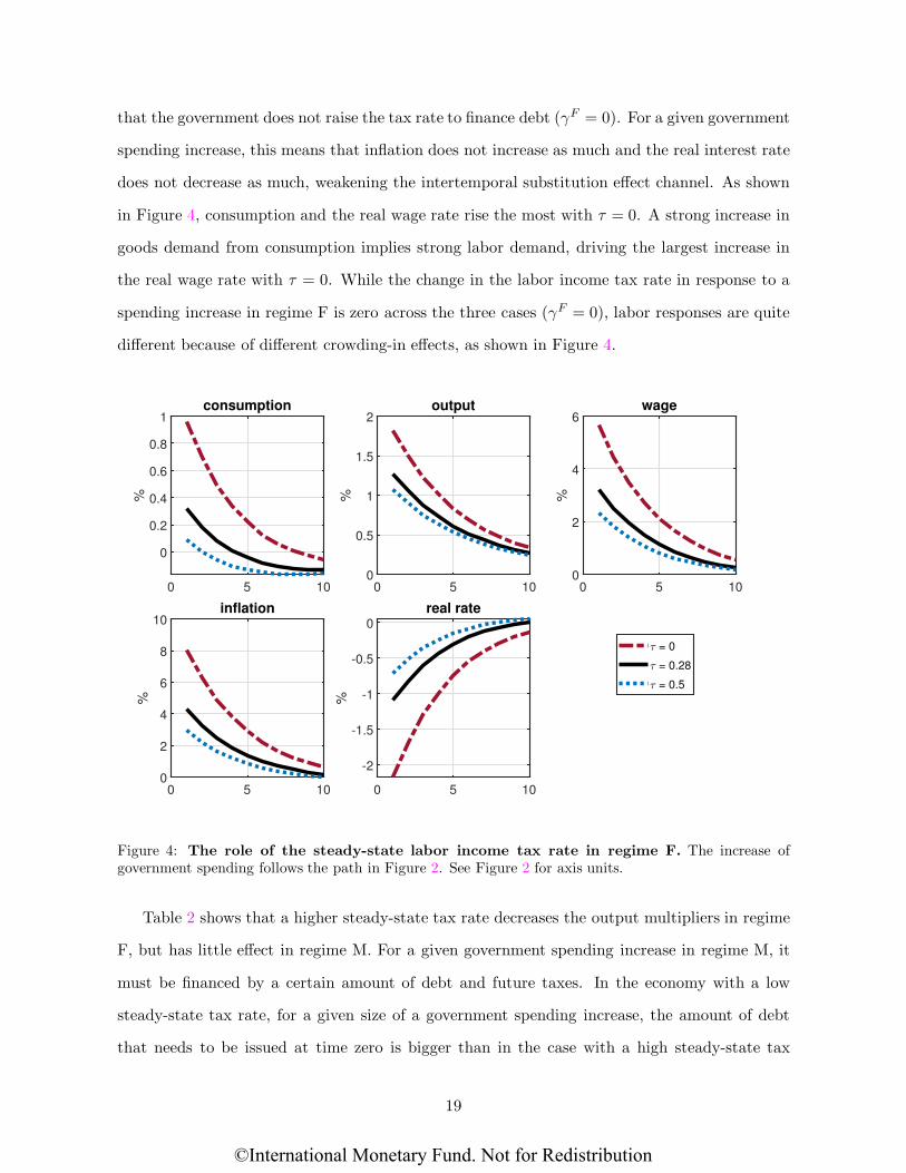
6.3 Government Debt in the Steady State

The left panel of Figure 10 plots the impact output multipliers as a function of the steady-

state debt-to-output ratio. To keep the economic structure as close as possible across the

economies under comparison, we only allow non-distorting steady-state transfers to vary to

satisfy the government budget constraint; all other parameters and steady-state values are set

to those in the baseline calibration (Table 2.4).

In regime M, we find almost no change in the impact output multipliers. Regardless of the

steady-state debt ratio, the crowding-out effect in regime M depends mainly on the amount

of additional debt and thus the amount of taxes eventually need to be raised to financing

government spending, determining the strength of negative wealth effects. As a result, the stock

of existing steady-state debt does not matter much for government spending effects in regime

M.

In regime F, instead, the multiplier decreases as the steady-state debt-to-output ratio in-

creases. Similar to an initial high-debt state (as analyzed in Section 3.2), given a fixed amount

of government spending to be financed by inflation, a higher steady-state debt ratio (which is also

the initial debt in the current simulation) provides a higher nominal base, so inflation increases

by less than in the case of low steady-state debt. As a result, the intertemporal substitution

effect is smaller and so is the output multiplier.

31


0 0.5 1 1.5 2

b/4y, s.s. debt-to-GDP

0.5

0.6

0.7

0.8

0.9

1

1.1

1.2

1.3

1.4

1.5

outp

ut m

ultip

lier

0 0.1 0.2 0.3 0.4 0.5

: s.s. labor tax rate

0.5

1

1.5

2

outp

ut m

ultip

lier

Regime M

Regime F

Figure 10: Sensitivity analysis: steady-state indebtedness vs. labor income tax rates. Theplots present the impact output multipliers. Except for the steady-state values in the x-axes, otherparameters are held at the values of the baseline calibration.

Our result in regime F differs from Leeper et al. (2017), who find that the steady-state debt

ratio affects output multipliers only when government debt has longer maturity. We show that

with a fully nonlinear model, the steady-state debt-to-output ratio matters in regime F even

with only short-term debt.

6.4 The Labor Income Tax Rate in the Steady State

The right plot of Figure 10 complements the analysis in Section 3.3, and presents the impact

output multipliers as a function of the steady-state labor income tax rate in the two regimes.

When τ = 0, it amounts to the case of only lump-sum taxes, as studied in Davig and Leeper

(2011), and the impact output multiplier is the highest—around 1.8. In this case, an increase in

government spending must be completely financed by inflation, leading to the biggest inflation

response and crowding-in effect. When the steady-state tax rate increases, the multipliers de-

crease at a relatively large rate. Also, the flat line for regime M confirms that the steady-state

labor income tax rate does not play a role in the spending multipliers, as shown in Table 2. (See

Section 3.3 for the underlying reasons.)

32


7 Conclusion

In this paper, we study government spending effects under different monetary-fiscal policy

regimes in a nonlinear model that features regime switching and the potentially binding ZLB.

We find that government spending multipliers under passive monetary policy can be lower

because of higher debt levels, longer debt maturity, higher distorting tax rates, more responsive

monetary policy to inflation, and the existence of policy regime uncertainty. These results

provide plausible explanations why empirical evidence does not always support big government

spending multipliers under passive monetary policy or when nominal interest rates are low.

Among the various factors, policy regime uncertainty is particularly important in reducing

the expansionary effects of government spending in regime F. With expectations of switching to

regime M, multipliers in regime F decrease because the negative wealth effect in regime M spills

over into regime F. In particular, when agents expect that future policy regimes can switch to

regime M with an initial high debt ratio, government spending multipliers can fall much below

one. Also, policy uncertainty matters in regime M, because higher inflation expectations in

regime F spill overs into regime M, leading to higher real interest rates in regime M.

From the policy perspective, our analysis points out that government spending in regime F

may not always be a very effective stimulus in regime F. The result is relevant to the recent

discussion on the very different effects between money- and debt-financed government spending

in the literature. Although our framework prevents us from modeling money-financed spending,

the main mechanisms driving the different spending effects between the two regimes are very

similar to those driving different effects between money- and debt-financed government spending.

This implies that big government spending multipliers for money-financed spending can be

subject to the same factors that lower the multipliers in regime F, as analyzed in this paper.

33


References

Almunia, M., Benetrix, A., Eichengreen, B., O’Rourke, K. H., Rua, G., 2010. From Great Re-

pression to Great Credit Crisis: Similarities, differences and lessons. Economic Policy 25 (62),

219–265.

Battistini, N., Callegari, G., Zavalloni, L., 2019. Dynamic fiscal limits and monetary-fiscal policy

interactions. Working Paper Series 2268, European Central Bank.

Beck-Friis, P., Willems, T., 2017. Dissecting fiscal multipliers under the fiscal theory of the price

level. European Economic Review 95, 62–83.

Bi, H., Shen, W., Yang, S.-C. S., 2016. Debt-dependent effects of fiscal expansions. European

Economic Review 88, 142–157.

Bianchi, F., Melosi, L., 2017. Escaping the Great Recession. American Economic Review 107 (4),

1030–1058.

Bianchi, F., Melosi, L., 2019. The dire effects of the lack of monetary and fiscal coordination.

Journal of Monetary Economics 104, 1–22.

Broner, F., Clancy, D., Martin, A., Erce, A., 2018. Fiscal multipliers and foreign holdings of

public debt. European Stability Mechanism Working Paper 30,.

Calvo, G. A., 1983. Staggered prices in a utility maxmimizing model. Journal of Monetary

Economics 12 (3), 383–398.

Canzoneri, M., Collard, F., Dellas, H., Diba, B., 2016. Fiscal multipliers in recessions. The

Economic Journal 590 (February), 75–108.

Christiano, L. J., Eichenbaum, M., Rebelo, S., 2011. When is the government spending multiplier

large? Journal of Political Economy 119 (1), 78–121.

Cogan, J. F., Cwik, T., Taylor, J. B., Wieland, V., 2010. New Keynesian versus old Keynesian

government spending multipliers. Journal of Economic Dynamics and Control 34 (3), 281–295.

34


Coleman, II, W. J., 1991. Equilibrium in a production economy with an income tax. Economet-

rica 59 (4), 1091–1104.

Davig, T., 2004. Regime-switching debt and taxation. Journal of Monetary Economics 51 (4),

837–859.

Davig, T., Leeper, E. M., 2006. Fluctuating Macro Policies and the Fiscal Theory. In NBER

Macroeconomic Annual 2006, edited by D. Acemoglu, K. Rogoff, and M. Woodford,. MIT

Press, Cambridge, MA.

Davig, T., Leeper, E. M., 2007. Generalizing the Taylor principle. American Economic Review

97 (3), 607–635.

Davig, T., Leeper, E. M., 2011. Monetary-fiscal policy interactions and fiscal stimulus. European

Economic Review 55 (2), 211–227.

Drautzburg, T., Uhlig, H., 2015. Fiscal stimulus and distortionary taxation. Review of Economic

Dynamics 18 (4), 894–920.

Dupor, B., Li, R., 2015. The expected inflation channel of government spending in the postwar

U.S. European Economic Review 74 (February), 36–56.

Dupor, W., Li, J., Li, R., 2018. Sticky wages, monetary policy and fiscal policy multipliers.

Working Paper 2017-007A, Federal Reserve Bank of St. Louis.

Eggertsson, G., Woodford, M., 2003. The zero bound on interest rates and optimal monetary

policy. Brookings Papers on Economic Activity 1, 139–211.

Eggertsson, G., Woodford, M., 2006. Optimal Monetary and Fiscal Policy in a Liquidity Trap.

Eggertsson, G. B., Singh, S. R., 2019. Log-linear approxiation versus an exact solution at the

ZLB in the New Keyesian model. Journal of Economic Dynamics and Control 105 (August),

21–43.

English, W., Erceg, C. J., Lopez-Salido, D., 2017. Money-financed fiscal programs: a cautionary

tale. Hutchins Center Working Paper 31, Brookings, Washington, D.C.

35


Erceg, C. J., Linde, J., 2014. Is there a fiscal free lunch in a liquidity trap? Journal of the

European Economic Association 12 (1), 73–107.

Fernandez-Villaverde, J., Gordon, G., Guerron-Quintana, P., Rubio-Ramirez, J. F., 2015. Non-

linear adventures at the zero lower bound. Journal of Economic Dynamics and Control 57,

182–204.

Forni, L., Monteforte, L., Sessa, L., 2009. The general equilibrium effects of fiscal policy: Esti-

mates for the e uro area. Journal of Public Economics 93 (3-4), 559–585.

Galı, J., forthcoming. The effects of a money-financed fiscal stimulus. Journal of Monetary

Economics.

Greenwood, J., Hercowitz, Z., Huffman, G. W., 1988. Investment, capacity utilization, and the

real business cycle. American Economic Review 78 (3), 402–417.

Ilzetzki, E., Mendoza, E. G., Vegh, C. A., 2013. How big (small?) are fiscal multipliers? Journal

of Monetary Economics 60 (2), 239–254.

International Monetary Fund, 2019a. Fiscal monitor. Chapter 1. Fiscal Policy for a Changing

Global Economy, April, Washington, D.C.

International Monetary Fund, 2019b. World Economic Outlook, April. Chapter 1: Global

Prospects and Policies, Washington, D.C.

Jacobson, M. M., Leeper, E. M., Preston, B., 2019. Recovery of 1933. NBER Working Paper

25629, National Bureau of Economic Research.

Kim, S., 2003. Structural shocks and the fiscal theory of the price level in the sitcky price model.

Macroeconomic Dynamics 7 (5), 759–782.

Kirchner, M., Cimadomo, J., Hauptmeier, S., 2010. Transmission of government spending shocks

in the euro area time variation and driving forces. Working Paper Series No. 1219, European

Central Bank.

Leeper, E. M., 1991. Equilibria under ‘active’ and ‘passive’ monetary and fiscal policies. Journal

of Monetary Economics 27 (1), 129–147.

36


Leeper, E. M., Traum, N., Walker, T. B., 2017. Clearing up the fiscal multiplier morass: Prior

and posterior analysis. American Economic Review 107 (8), 2409–2454.

Miao, J., Ngo, P. V., forthcoming. Does Calvo meet Rotemberg at the zero lower bound? Macroe-

conomic Dynamics.

Michaillat, P., 2014. A theory of countercylical government multiplier. American Economic Jour-

nal: Macroeconomics 6 (1), 190–217.

Miyamoto, W., Nguyen, T. L., Sergeyev, D., 2018. Government spending multipliers under the

zero lower bound: Evidence from japan. American Economic Journal: Macroeconomics 10 (3),

247–277.

Nickel, C., Tudyka, A., 2014. Fiscal stimulus in times of high debt: Reconsidering multipliers

and twin deficits. Journal of Money, Credit and Banking 46 (7), 1313–1344.

Office of Debt Management, 2018. Treasury presentation to treasury borrowing advisory com-

mittee. U.S. Treasury Department.

Ramey, V. A., 2011. Identifying government spending shocks: It’s all in the timing. Quarterly

Journal of Economics 126 (1), 1–50.

Ramey, V. A., Zubairy, S., 2018. Government spending multipliers in good times and in bad:

Evidence from U.S. historical data. Journal of Political Economy 126 (2), 850–901.

Rotemberg, J. J., 1982. Sticky prices in the United States. Journal of Political Economy 90 (De-

cember), 1187–1211.

Shen, W., Yang, S.-C. S., 2018. Downward nominal wage rigidity and state-dependent govern-

ment spending multipliers. Journal of Monetary Economics 98 (October), 11–26.

Shen, W., Yang, S.-C. S., Zanna, L.-F., 2018. Government spending effects in low-income coun-

tries. Journal of Development Economics 133 (July), 201–219.

Smets, F., Wouters, R., 2007. Shocks and frictions in US business cycles: A Bayesian DSGE

approach. American Economic Review 97 (3), 586–606.

37


Tauchen, 1986. Finite state Markov-chain approximations to univariate and vector autoregres-

sions. Economics Letters 20 (2), 177–181.

Traum, N., Yang, S.-C. S., 2011. Monetary and fiscal policy interactions in the post-war U.S.

European Economic Review 55 (1), 140–164.

Traum, N., Yang, S.-C. S., 2015. When does government debt crowd out investment? Journal

of Applied Econometrics 30, 24–45.

Wieland, J., 2018. State-dependence of the zero lower bound government spending multiplier.

Manuscript, University of California, San Diego.

Woodford, M., 2001. Fiscal requirements for price stability. Journal of Money, Credit and Bank-

ing 33 (3), 669–728.

Woodford, M., 2011. Simple analytics of the government expenditure multiplier. American Eco-

nomic Journal: Macroeconomics 3 (1), 1–35.

38


Appendices

A Equilibrium System

Households’ optimality conditions:

λt = Uct (A.1)

(1 − τ lt)wtλt = −Unt (A.2)

Qt = Et

[

βλt+1

λt

1 +Qt+1(1 − κ)

πt+1

]

(A.3)

1

Rft

= Et

[

βλt+1

λt

1

πt+1

]

(A.4)

ct +Qt(

bt −(1− κ)bt−1

πt

)

=bt−1

πt+ (1 − τ lt)wtnt + Υt + ξt + zt (A.5)

Firms’ optimality conditions:

ψ

(

πt

π∗− 1

)

πt

π∗= (1 − θ) + θmct + βψEt

[

λt+1

λt

yt+1

yt

πt+1

π∗

(

πt+1

π∗− 1

)]

(A.6)

mct =wt

At(A.7)

yt = Atnt (A.8)

Υt =[

1 −mct −ψ

2

( πt

π∗− 1

)2]yt (A.9)

Government budget constraint and policy rules:

Qt(

bt −(1 − κ)bt−1

πt

)

+ τ ltwtnt =bt−1

πt+ gt + zt (A.10)

τt = τ + γ(bt−1 − b) ·R

R+ (1− κ)(A.11)

Rt = max

{

1, R · (πt

π∗)απ

}

(A.12)

Aggregate resource constraint:

yt = ct + gt (A.13)

39


Exogenous variables:

consumption taste: νt = ρννt−1 + ενt , ενt ∼ N (0, σ2ν) (A.14)

government spending: lngt

g= ρg ln

gt−1

g+ ε

gt , ε

gt ∼ N (0, σ2

g) (A.15)

The policy regime indicator, st, follows a Markov process with the following transition prob-

abilities: P(st = M |st−1 = M) = ρMM and P(st = F |st−1 = F ) = ρFF .

B Deterministic Steady State

The deterministic steady state is characterized by the following equations:

1

R=

β

π∗(B.1)

Q =β

π∗ − β(1 − κ)(B.2)

mc =θ − 1

θ(B.3)

θ − 1

θτ −

g

y−z

y=

1 − β

π∗ − β(1− κ)·b

y(B.4)

c+ g = y = n (B.5)

c−σ · (1 − τ) ·mc = χ · yϕ = χ · nϕ. (B.6)

The average duration of the government bonds is

R

R+ (1 − κ)=

π∗

π∗ − β(1− κ). (B.7)

The government debt-to-annual output ratio is

b+Q(1− κ)b

4y=

Rκ+(R−1) · b

4y. (B.8)

The left hand side of (B.8) is the market value of outstanding debt, and the right hand side is the

face value of outstanding debt. The market value of debt is the same as the face value of debt at

40


the steady state.22 The steady-state market value of debt with decaying coupons is sometimes

defined as Qb4y in the literature. If we adopt this definition, the short-term debt case cannot

be nested, because b is not exactly outstanding liabilities of a long-term debt. Quantitatively,

the difference in the two definitions of the debt market value is negligible. Here we make the

modification to nest the short-term debt case within a general expression.

C Computational Algorithm

The model is solved with Euler equation iteration as described in Coleman (1991), which

finds the fixed point of the Euler equations directly. Specifically, it makes initial guesses for

future policy functions and iterates backwards to solve for the true policy functions. In this

paper, the method is implemented in Fortran 90 and paralleled with OpenMP.23

Given the equilibrium system in Appendix A for the baseline economy, the set of the pol-

icy functions to be solved is {λ(bt−1; St), Q(bt−1; St), π(bt−1; St)}, where bt−1 is the endogenous

state,24 and the exogenous state vector, St, consists of the exogenous variables, {νt, gt}, and the

policy regime indicator, st.

The equilibrium conditions used to solve the model consist of

Rft = max

{

1,(

Rft−1

)ρrf (

Rf(πt

π∗)απ

)1−ρrf

eεrft

}

(C.1)

(ct − νt)−σ = λt (C.2)

nt = ct + gt (C.3)

τt = τ + γ(bt−1 − b) ·1 + r

κ+ r(C.4)

(1 − τ lt)wtλt = χnϕt (C.5)

mct = wt (C.6)

bt =

bt−1

πt+ gt + zt − τ ltwtnt

Qt+

(1− κ)bt−1

πt. (C.7)

22This can be easily shown by plugging in the steady-state price bond price, Q.23Replication files can be downloaded from https://sites.google.com/view/rmao/research?authuser=0.24For the regime switching case with time-varying switching probability, πt−1 is also a state variable. The

algorithm is similar; the only difference is that when calculating expectation, the switching probability is calculatedby equation (4.2).

41


https://sites.google.com/view/rmao/research?authuser=0

The equations used for updating the policy functions consist of

λt

Rft

= βEt

[

λt+1

πt+1

]

(C.8)

λtQt = βEt

[

λt+1 ·

(

(1 +Qt+1(1 − κ))

πt+1

]

(C.9)

ψ

(

πt

π∗− 1

)

πt

π∗= (1− θ) + θmct + βψEt

[

λt+1

λt

nt+1

nt

πt+1

π∗

(

πt+1

π∗− 1

)]

. (C.10)

The solution algorithm is described below.

1. Discretize the state space using Tauchen (1986).

2. Guess the form of the policy functions: λ(1)(

bt−1; St)

, Q(1)(

bt−1; St)

, and π(1)(

bt−1; St)

.

3. For each state, plug the initial guesses to the system of optimality conditions, (C.1)– (C.7),

to calculate Rft , ct, nt, wt, mct, and bt.

4. With bt from the last step, evaluate the expectations on the right hand side of (C.8)–

(C.10) by calculating next period’s policy values with the guessed policy functional forms:

λ(1)(

bt; St+1

)

, Q(1)(

bt; St+1

)

, and π(1)(

bt; St+1

)

.

5. Solve for the policy functions—λ(2), Q(2), and π(2)—by solving a three-dimensional root-

finding problem with (C.8)–(C.10).

6. Check convergence. If max{‖λ(1) − λ(2)‖, ‖Q(1) − Q(2)‖, ‖π(1) − π(2)‖} < 10−6, then

{λ(2), Q(2), π(2)} is the final solution; else update λ(1), Q(1), and π(1) with λ(2), Q(2), and

π(2), and repeat steps 2-4 until the conversion criterion is satisfied.

When solving the model, we use linear interpolation for policy function approximations.

Since the state space is discretized with Tauchen (1986), numerical expectations are calculated

accordingly. We also use quadrature to evaluate numerical integration as a robustness check, and

the differences are small for this model. The root-finding routine we use is a Fortran translation

from csolve.m by Sims.25

Lastly, there are a few remarks on model convergence. Regime M usually converges to the

equilibrium faster than Regime F. One can start with the steady-state values or the solution

25The code can be downloaded from http://sims.princeton.edu/yftp/optimize/.

42


http://sims.princeton.edu/yftp/optimize/

from the log-linearized model as the initial guesses. When solving the model in regime F with no

tax response to debt (γF = 0), we first solve the model under a small but non-zero value of γF

and then use the solution as the initial guess for the case for γF = 0. Similarly, when solving for

the equilibrium with regime switching or a highly persistent government spending process, we

use the solutions of the fixed regime case or a less persistent spending process as initial guesses.

43


Documents

WP/20/ - elibrary.imf.org