Writing Finance Papers Using LATEX∗

RS: Notes like thisappear throughoutthe document andare created using thetodonotes package (seeSection 5.6).

RS: Notes like thisappear throughoutthe document andare created using thetodonotes package (seeSection 5.6).Richard Stanton†

June 19, 2012, 15:24 RS: Including the cur-rent time helps to locatethe latest printout inthat huge pile on yourdesk when you createmany versions of a pa-per during the day (seedatetime package, Sec-tion 5.7).

RS: Including the cur-rent time helps to locatethe latest printout inthat huge pile on yourdesk when you createmany versions of a pa-per during the day (seedatetime package, Sec-tion 5.7).

Abstract

This document provides some recommendations for efficiently writing finance pa-pers using LATEX and related tools, based on techniques that have made me moreproductive over the years. It also contains the necessary LATEX style files and BibTEXformat files (along with sample paper outlines) for making your paper and bibliog-raphy match the formats required by the Journal of Finance, Journal of FinancialEconomics, and Review of Financial Studies. The source file, texintro.tex, andvarious additional included files are important parts of this document.

∗Comments and suggestions on this document are welcome. I am grateful to Jennifer Carpenter andJohan Walden for valuable input (even if some of it was inadvertent). I am also grateful to Tobias Oetiker

for writing the example environment, which I use liberally in this document. INCLUDES NOTES.

RS: I like to have thison the front page to re-duce the likelihood thatthe paper will go backto the journal completewith all my insultingcomments about the ref-eree.

RS: I like to have thison the front page to re-duce the likelihood thatthe paper will go backto the journal completewith all my insultingcomments about the ref-eree.

†Haas School of Business, U.C. Berkeley, 545 Student Services Building #1900, Berkeley, CA 94720-1900,phone: 510-642-7382, fax: 510-643-1412, e-mail: stanton@haas.berkeley.edu.

Contents RS: Every entry in thetable of contents is aclickable hyperlink (seehyperref package, Sec-tion 5.10)

RS: Every entry in thetable of contents is aclickable hyperlink (seehyperref package, Sec-tion 5.10)

1 Introduction 3

2 Installing LATEX 4

3 Entering Text 83.1 Spaces and line breaks . . . . . . . . . . . . . . . . . . . . . . . . . . . . . . 83.2 Sections and subsections . . . . . . . . . . . . . . . . . . . . . . . . . . . . . 83.3 Emphasizing text . . . . . . . . . . . . . . . . . . . . . . . . . . . . . . . . . 93.4 Tables . . . . . . . . . . . . . . . . . . . . . . . . . . . . . . . . . . . . . . . 93.5 Figures . . . . . . . . . . . . . . . . . . . . . . . . . . . . . . . . . . . . . . . 9

4 Entering Mathematical Expressions 94.1 Inline versus displayed expressions (unnumbered) . . . . . . . . . . . . . . . 104.2 Numbered equations . . . . . . . . . . . . . . . . . . . . . . . . . . . . . . . 104.3 Spacing in mathematical expressions . . . . . . . . . . . . . . . . . . . . . . 114.4 Long equations . . . . . . . . . . . . . . . . . . . . . . . . . . . . . . . . . . 124.5 Text inside mathematical expressions . . . . . . . . . . . . . . . . . . . . . . 124.6 Brackets . . . . . . . . . . . . . . . . . . . . . . . . . . . . . . . . . . . . . . 124.7 Arrays . . . . . . . . . . . . . . . . . . . . . . . . . . . . . . . . . . . . . . . 134.8 Defining new operators . . . . . . . . . . . . . . . . . . . . . . . . . . . . . . 134.9 Theorems, etc. . . . . . . . . . . . . . . . . . . . . . . . . . . . . . . . . . . 13

5 Useful LATEX Packages 135.1 Installing packages . . . . . . . . . . . . . . . . . . . . . . . . . . . . . . . . 145.2 Changing line spacing: setspace . . . . . . . . . . . . . . . . . . . . . . . . 165.3 Including figures: graphicx . . . . . . . . . . . . . . . . . . . . . . . . . . . 165.4 Mathematical typesetting: amsmath . . . . . . . . . . . . . . . . . . . . . . . 175.5 Setting page margins: geometry . . . . . . . . . . . . . . . . . . . . . . . . . 195.6 Inserting notes: todonotes . . . . . . . . . . . . . . . . . . . . . . . . . . . . 195.7 Printing date and time: datetime . . . . . . . . . . . . . . . . . . . . . . . . 205.8 Multiple versions from one file: versionPO . . . . . . . . . . . . . . . . . . . 215.9 List formatting: enumitem . . . . . . . . . . . . . . . . . . . . . . . . . . . . 225.10 URLs and hyperlinks: hyperref . . . . . . . . . . . . . . . . . . . . . . . . . 225.11 Landscape and subfigures: rotating and subfigure . . . . . . . . . . . . . 235.12 Other useful packages . . . . . . . . . . . . . . . . . . . . . . . . . . . . . . . 24

6 Citations and Bibliographies 266.1 BibTEX . . . . . . . . . . . . . . . . . . . . . . . . . . . . . . . . . . . . . . 276.2 The BibTEX database . . . . . . . . . . . . . . . . . . . . . . . . . . . . . . 286.3 Telling BibTEX where to find the database . . . . . . . . . . . . . . . . . . . 296.4 Formatting the bibliography: natbib and custom-bib . . . . . . . . . . . . 29

1

7 Journal-Specific Document Formatting 307.1 Formatting the bibliography . . . . . . . . . . . . . . . . . . . . . . . . . . . 317.2 Formatting the text . . . . . . . . . . . . . . . . . . . . . . . . . . . . . . . . 31

8 Working with Others: Version Control Systems 328.1 Public hosting of DVCS repositories . . . . . . . . . . . . . . . . . . . . . . . 348.2 This project’s Bitbucket repository . . . . . . . . . . . . . . . . . . . . . . . 34

2

1 Introduction

LATEX is a document typesetting system, based on Knuth’s program TEX (see Knuth, 1984), RS: By default, LATEXsets huge margins. Cus-tomize them easily usingthe geometry package(see Section 5.5).

RS: By default, LATEXsets huge margins. Cus-tomize them easily usingthe geometry package(see Section 5.5).

which makes it relatively simple to produce papers with high-quality equations and error-

free cross-references to equations, tables, and figures, and to handle creation and formatting

of bibliographies and citations.1 This document explains the basics of installing and using

LATEX to produce high-quality papers,2 and presents a number of suggestions for tools and

techniques that make me more productive when I write papers, along with instructions and

sample files for formatting your papers to match the requirements of the Journal of Finance,

Journal of Financial Economics, and Review of Financial Studies.

This document is not intended to be a comprehensive overview of LATEX. If you’re starting

from scratch, one very popular reference, free to download, is the “Not So Short Introduction

to LATEX 2ε” (Oetiker, Partl, Hyna, and Schlegl, 2011). There are also some excellent books RS: Section 6 dealswith creating citationsand bibliographies usingBibTEX.

RS: Section 6 dealswith creating citationsand bibliographies usingBibTEX.on LATEX. Standard references include Lamport (1994), written by the original author of

LATEX; Kopka and Daly (2003), a more recent, popular introductory text; and Mittelbach,

Goossens, Braams, Carlisle, and Rowley (2004), an excellent reference on both LATEX itself

and many of the additional packages that have been created since LATEX was created (the

authors of this book are some of the main developers of LATEX).3

Creation of a document using LATEX is a two-step process:

1. Create a LATEX source file, usually with the extension .tex, containing your text plus

commands that tell LATEX how to format your document.4 RS: By default, LATEXinserts more space be-tween list items than this(see enumitem package,Section 5.9).

RS: By default, LATEXinserts more space be-tween list items than this(see enumitem package,Section 5.9).

2. Process the .tex file to create the final PDF file.5

1Plenty of people use word processors for writing papers instead. This makes no sense to me, but ratherthan engage in a debate, I’ll just note that if you use Word this document is probably not going to be veryuseful to you.

2I’m talking about the quality of the typesetting here. The intellectual quality is up to you.3I own and refer to all of these books, especially Mittelbach et al. (2004), and I originally learned LATEX

from Lamport (1994). You can also find other references at http://www.ctan.org/starter.html. However,I find that nowadays I use Google more than any other reference.

4For example, the source for this document is called texintro.tex. Unlike word-processor files, LATEXfiles are plain text, with no special control codes. This makes them easily portable from one machine (orarchitecture or OS) to another, easy to view using any plain-text file viewer, and also means that you standa decent chance of being able to rescue a lot of your material if the file accidentally gets corrupted, say by amisbehaving word processor or a disk failure. Not that files get corrupted all that often, of course, but justin case, it’s nice to know. This also makes it easy to keep track of your work using a Version Control System(see Section 8).

5Before PDF became standard, it was usual for the .tex file to be processed to a .dvi (Device Independent)file, which was then further processed to a printable format using a printer-specific executable (e.g., dvipsfor Postscript or dvilj for an HP Laserjet). To create a PDF file, you would 1) run latex to create a .dvifile, 2) run dvips to convert the .dvi file into a Postscript file, and 3) run Adobe Distiller (or Ghostscript) toconvert the PS file to PDF. Nowadays this is usually done in one step (using the pdflatex program behindthe scenes). Yes, I know you still insist on using dvips, Johan, though I have no idea why. . . .

3

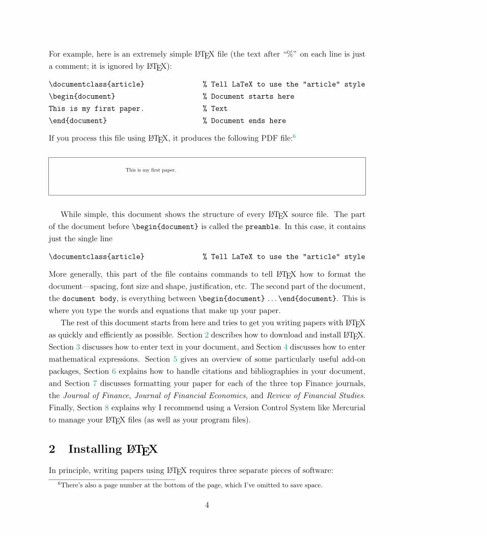
For example, here is an extremely simple LATEX file (the text after “%” on each line is just

a comment; it is ignored by LATEX):

\documentclass{article} % Tell LaTeX to use the "article" style

\begin{document} % Document starts here

This is my first paper. % Text

\end{document} % Document ends here

If you process this file using LATEX, it produces the following PDF file:6

This is my first paper.

1

While simple, this document shows the structure of every LATEX source file. The part

of the document before \begin{document} is called the preamble. In this case, it contains

just the single line

\documentclass{article} % Tell LaTeX to use the "article" style

More generally, this part of the file contains commands to tell LATEX how to format the

document—spacing, font size and shape, justification, etc. The second part of the document,

the document body, is everything between \begin{document} . . . \end{document}. This is

where you type the words and equations that make up your paper.

The rest of this document starts from here and tries to get you writing papers with LATEX

as quickly and efficiently as possible. Section 2 describes how to download and install LATEX.

Section 3 discusses how to enter text in your document, and Section 4 discusses how to enter

mathematical expressions. Section 5 gives an overview of some particularly useful add-on

packages, Section 6 explains how to handle citations and bibliographies in your document,

and Section 7 discusses formatting your paper for each of the three top Finance journals,

the Journal of Finance, Journal of Financial Economics, and Review of Financial Studies.

Finally, Section 8 explains why I recommend using a Version Control System like Mercurial

to manage your LATEX files (as well as your program files).

2 Installing LATEX

In principle, writing papers using LATEX requires three separate pieces of software:

6There’s also a page number at the bottom of the page, which I’ve omitted to save space.

4

1. A text editor to edit the .tex source file.

2. TEX/LATEX software to process your source file and create the final PDF file.

3. A PDF viewer so you can see the output.

While you can install three separate pieces of software, it is much simpler to use a LATEX

installation that comes with a “front-end” program, which seamlessly integrates all of these

pieces into one so you never have to think about the different steps involved.7 The standard

LATEX installations for Windows and OS X both come with a good front-end program:

OS Installation Name Front end URL

Windows MikTeX TeXworks http://miktex.org

OS X MacTeX TeXShop http://www.tug.org/mactex.

To install one of these on your system, go to the URL listed above (you can click on the

link) and follow the installation instructions.8

Creating a document with either TeXworks or TeXShop involves loading the .tex file,

editing it until you’re happy with it, then pressing a button to create the PDF file, which

will also be displayed on the screen. Figure 1 shows how the TeXworks environment looks

when editing the test file from above. Figure 2 shows the same for TeXShop. In both cases:

• Different syntactical elements are highlighted in different colors.

• Processing the .tex file to a PDF file entails just pressing a single button.9

• When there are errors, you can automatically be taken to the right place in the text.

• You can easily see which bit of the PDF file corresponds to which bit of the .tex file,

making editing easier.

7There is nothing to stop you switching to separate programs later, if you want. For example, I useEmacs (see http://www.gnu.org/software/emacs/) for editing .tex files (and for almost everything else inmy life), and either SumatraPDF (Windows—see http://blog.kowalczyk.info/software/sumatrapdf)or Skim (OS X—see http://skim-app.sourceforge.net/) to view the resulting PDF files.

8There seems to be a bug in the MikTeX installation, which causes MikTeX to be installed with a defaultA4 paper size regardless of what you ask for during the installation. This in turn causes pages to be offsetvertically by about an inch. You can get around this by setting fake margins in your document to compensate(yes, I mean you, Johan. . . ), but this will annoy coauthors who don’t suffer from this bug. Instead, changethe default paper size manually after installing MikTeX:

• From the Windows program menu, select MikTeX 2.09→Maintenance (Admin)→ Settings (Admin).• Under “Paper” select “Letter (letterSize),” then press “Update formats” and press OK (see Figure 3).

9To do this manually from a command prompt, you typically have to run a series of commands, especiallyif you’re using BibTEX to handle your citations (see Section 6):pdflatex test

bibtex test

pdflatex test

pdflatex test

5

Fig

ure

1:S

imp

ledocu

ment

wit

hT

eX

work

s.Show

ssy

nta

xhig

hligh

ting

and

sim

ult

aneo

us

vie

wof

text

and

PD

Ffile

sRS:

To

inse

rtgra

phic

s,u

seth

e\i

ncludegraphics

com

man

d(s

eegraphicx

pack

age,

Sec

tion

5.3

).T

ocr

eate

ala

nd

scap

efi

gu

re,

use

thesidewaysfigure

envir

onm

ent

(see

rotating

pack

age,

Sec

tion

5.1

1).

6

Fig

ure

2:S

imp

ledocu

ment

wit

hT

eX

Shop.

Show

ssy

nta

xhig

hligh

ting

and

sim

ult

aneo

us

vie

wof

text

and

PD

Ffile

s.

7

3 Entering Text

3.1 Spaces and line breaks

Entering text in a LATEX document is pretty straightforward—just type it. A couple of

things to note if you’re used to a word processor (i.e., if you are between 3 and 90 years old):

i. LATEX doesn’t care if you use one or several spaces or how often you insert a line break,

and ii. a completely blank line tells LATEX to start a new paragraph.

Lots of spaces and

some line breaks, but \LaTeX\

doesn’t care.

A blank line tells \LaTeX\ to

start a new paragraph.

Lots of spaces and some line breaks, but LATEX

doesn’t care.

A blank line tells LATEX to start a new para-

graph.

LATEX automatically adds extra space at the end of a sentence. However, it gets confused

when a word in the middle of a sentence ends with a period. In this case, you can use

\ (backslash then space) to force LATEX to insert a regular intra-sentence space. For example,

I ran into Dr. Smith, who was walking

extremely rapidly. \\

I ran into Dr.\ Smith, who was walking

extremely rapidly.

I ran into Dr. Smith, who was walking ex-

tremely rapidly.

I ran into Dr. Smith, who was walking extremely

rapidly.

Another special space, ~, is used when we want to prevent a line break between two words,

such as between “Section”, “Equation”, etc., and the number that follows. For example,

It’s difficult to read this when

we allow ‘‘Section 3’’ to have a line

break in the middle.\\

It’s difficult to read this when

we allow ‘‘Section~3’’ to have a line

break in the middle.

It’s difficult to read this when we allow “Section

3” to have a line break in the middle.

It’s difficult to read this when we allow “Sec-

tion 3” to have a line break in the middle.

3.2 Sections and subsections

Start a new section or subsection using the commands \section and \subsection. E.g.,

8

\section{Section Title}

\subsection{Subsection title}

Some very uninteresting text\ldots

1 Section Title

1.1 Subsection title

Some very uninteresting text. . .

If you need them, there are also subsubsections, paragraphs, and subparagraphs:

\subsubsection{Subsubsection title}

\paragraph{Paragraph title}

This is a paragraph.

\subparagraph{Subparagraph title}

Yet more uninteresting text\ldots

1.1.1 Subsubsection title

Paragraph title This is a paragraph.

Subparagraph title Yet more uninterest-

ing text. . .

If you want any of these not to be numbered, add an asterisk after the command name, e.g.,

\section*{An Untitled Section}.

Note that these instructions tell LATEX about the logical structure of the document (e.g.,

“I want to start a new section here”) but not about the formatting that goes along with it

(e.g., “Format this left-justified in Times-Roman 12 point”), which LATEX takes care of by

itself. This is a general feature of LATEX, which means that you spend most of your time

thinking about what you’re writing rather than about how to format your paper.

3.3 Emphasizing text

3.4 Tables

3.5 Figures

4 Entering Mathematical Expressions

LATEX excels at typesetting mathematical expressions. You can do most things using just

the capabilities built in to basic LATEX, but there are some very useful additional features

provided by the amsmath package (see Section 5.4), which I recommend loading into every

document by including the line

\includepackage{amsmath}

9

in the preamble. This document mentions some of the additional capabilities provided by

the amsmath package, but for full details you should see the package documentation, avail-

able at http://www.tug.org/texlive/Contents/live/texmf-dist/doc/latex/amsmath/

amsldoc.pdf.

4.1 Inline versus displayed expressions (unnumbered)

There are two different ways to display mathematical expressions in LATEX:

1. Inline: The expression appears as part of the paragraph if surrounded by (single) dollar

signs, $ . . . $, or (equivalently) \( . . . \). For example,

Of course, $e^{i\pi} + 1 = $

\( \lim_{x \rightarrow 0}

\frac{\sin(x)}{x} - 1 = 0 \).

Of course, eiπ + 1 = limx→0sin(x)x − 1 = 0.

2. Display: The expression appears on a separate line, with more generous vertical spacing,

if surrounded by $$ . . . $$ or (equivalently) \[ . . . \]. For example,

Here is a displayed equation:

$$ E = \frac{mv^2}{2}. $$

Here is a displayed equation:

E =mv2

2.

Here is another:

\[ \left[\int_0^\frac{\pi}{2}

\frac{\cos(x)}{2} \, dx\right]^3 =

\frac{1}{8}. \]

Here is another:[∫ π2

0

cos(x)

2dx

]3

=1

8.

4.2 Numbered equations

LATEX also has several environments that create numbered equations. For example,

A numbered equation:

\begin{equation}

E = mc^2.

\label{eq:Einstein}

\end{equation}

A numbered equation:

E = mc2. (1)

10

Aligned, numbered equations:

\begin{align}

\sum_{i=1}^n i &=

\frac{n(n+1)}{2}; \\

\sum_{i=1}^n i^2 &=

\frac{n(n+1)(2n+1)}{6}.

\end{align}

Aligned, numbered equations:

n∑i=1

i =n(n+ 1)

2; (2)

n∑i=1

i2 =n(n+ 1)(2n+ 1)

6. (3)

To refer to equations in the text, use either \ref or \eqref:10

Eq.~\eqref{eq:Einstein} \ldots \\

Eq.~(\ref{eq:Einstein}) \ldots

Eq. (1) . . .

Eq. (1) . . .

4.3 Spacing in mathematical expressions

We saw above (Section 3.1) that LATEX doesn’t care much about how much whitespace you

have in your text; one space is the same as one hundred. LATEX cares even less about

whitespace in equations—it ignores spaces completely (something that’s easy to forget). For

example, suppose you wanted to typeset the equation

dS

S= mdt + s dZ.

To create a space between, say, the m and the dt, the obvious thing to try is to insert a

space in the text file, but this looks a lot better in the .tex source than it does in the final

document. . . :

\[

\frac{dS}{S} = m dt + s dZ.

\]

dS

S= mdt+ sdZ.

LATEX completely ignores those spaces, making the right hand side very hard to interpret.

You have to tell LATEX explicitly when you want to insert some space in an equation, in this

case using the “thinspace” command, \,:

\[

\frac{dS}{S} = m\,dt + s\,dZ.

\]

dS

S= mdt+ s dZ.

10The \eqref command and align environment require the amsmath package (see Section 5.4).

11

4.4 Long equations

Sometimes an equation or expression is too long to fit onto a single line. The amsmath

package (see Section 5.4) provides several options to deal with this, notably the multline

and split environments. For example,

\begin{multline}

a+b+c+d+e+f+g+ \\

h+i+j+k+l+m+n

\end{multline}

a+ b+ c+ d+ e+ f + g+

h+ i+ j + k + l +m+ n (4)

\begin{align}

y & = mx + c. \\

\begin{split}

a & = b+c+d+e+f+g\\

& \quad -h+i+j+k+l

\end{split}

\end{align}

y = mx+ c. (5)

a = b+ c+ d+ e+ f + g

− h+ i+ j + k + l(6)

4.5 Text inside mathematical expressions

If you want to put text inside a mathematical expression, enclose it in either \mbox{} or

\text{}. These are very similar, though the latter requires the amsmath package to be

loaded. One advantage of \text{}, however, is that it knows how to adjust the font size

when used as part of a subscript. For example,

\begin{align*}

A_{\mbox{font too big}} &= 1

\mbox{ in most cases.} \\

A_{\text{font OK}} &= 1

\text{ in most cases.}

\end{align*}

Afont too big = 1 in most cases.

Afont OK = 1 in most cases.

4.6 Brackets

It is often necessary to put brackets around mathematical expressions. For small expressions,

this can be done (almost) the obvious way, using ( . . . ), [ . . . ], or \{ . . . \} (but note that

you need a backslash before { or }). For example,

12

\[

(a+b)+[c+d]+\{e+f\}.

\]

(a+ b) + [c+ d] + {e+ f}.

However, this doesn’t work so well if the expressions inside the brackets are taller than a

single character. For example, the following expression really needs larger brackets:

\[

(\frac{a}{b})+

\{\frac{c^{[d+\frac{e^2}{2}]}}{f}\}

\]

(a

b) + {c

[d+ e2

2]

f}

LATEX has various commands for manually setting a larger bracket size, but in the vast

majority of cases you can just let LATEX set the bracket size automatically by using \left(,

\right), etc. For example,

\[

\left(\frac{a}{b}\right)+

\left\{\frac{c^{\left[d+\frac{e^2}{2}

\right]}}{f}\right\}

\]

(ab

)+

c[d+ e2

2

]f

4.7 Arrays

4.8 Defining new operators

4.9 Theorems, etc.

5 Useful LATEX Packages

The standard LATEX distribution comes with a large number of extra “packages.” These are

files with the extension .sty, which allow you to customize the behavior of LATEX, either by

adding additional functionality or by changing the behavior of functions already defined.

Many of these packages are extremely useful. For example, if you want to include graphics

in your paper, you load the graphicx package (defined in the file graphicx.sty).

To use a package installed on your system, you use the command \usepackage. For

example, to load the graphicx package, you’d include the command

\usepackage{graphicx}

in the preamble to your document. Near the top of this file you’ll find the lines

13

\usepackage{setspace,graphicx,epstopdf,amsmath,versionPO}

\usepackage{marginnote,datetime,url,enumitem,subfigure,rotating}

These lines load some packages that I find particularly useful, and include in almost every

document I write. You can find full documentation on the Web, but here’s a brief description

of why each of these packages is so useful, with some brief examples illustrating their use.

Before that, however, a discussion of how to install them so LATEX knows where to find them.

5.1 Installing packages

It’s easy to use a package once it’s installed on your system, but what do you have to do to

install a package you haven’t used before? The usual answer is “nothing.” Nearly all of the

packages you’ll ever want (including nearly all the packages described in this document) are

installed as part of the LATEX distribution.11

5.1.1 Installing Non-Standard Packages

From time to time, you may want to use a package that is not part of the standard LATEX

distribution. One of the packages I use on a regular basis, versionPO, falls into this category,

and so do my customized journal-specific files, jf.sty, jfe.sty, and rfs.sty. One way to

use packages like this is just to copy them into the directory containing your project’s .tex

file, and they will automatically be found when you process it. However, this is not a great

solution, as you have to do it for every new project, and if you ever need to edit one of these

files, it’s very easy to lose track of the most recent version when you have dozens of copies

at various places on your disk.

A much better method is to install these files (once) somewhere LATEX will always know

where to find them. This does require a bit of work, but it only has to be done once. Let’s

illustrate this with the versionPO package included with this document.

1. The first thing you need to decide is where to put your extra .sty file(s). You could put

them in the same directory structure as the standard packages, but don’t do this!12

Instead, set up your own local directory tree. For example, on my Windows system,

I store extra packages in subdirectories under c:\RHS\texmf-local\tex\latex, and

on my Mac I use /Users/stanton/Library/texmf/tex/latex.13

11In some cases (e.g., MikTeX) you can choose not to install all packages, but to have the package managerinstall new packages for you whenever you ask to use them for the first time.

12When you next upgrade your installation, you’ll have to remember to copy them elsewhere (which alsomeans remembering which packages they were) to avoid losing them.

13This may seem complicated, but it follows the recommended TEX directory structure. You can pick

14

2. After creating the relevant directory, tell your LATEX installation where to find it.

• MikTeX 2.09:

– From the Windows program menu, select MikTeX 2.09 → Maintenance (Ad-

min) → Settings (Admin).

– Click on the “Roots” tab, click “Add,” and select the appropriate directory

structure (in my case, this is c:\RHS\texmf-local).14

• TeX Live (MacTeX):

– If you chose the same directory as I did (~/Library/texmf/tex/latex, where

~ denotes your own home directory, e.g., /Users/stanton), LATEX will auto-

matically look for files there and in all subdirectories, so you don’t need to

do anything else here.

Note: Both of these steps only need to be done once for a given LATEX installation. The

next steps need to be performed for every non-standard package you install.

3. Copy any new .sty files into the directory structure you just created. For example,

c:\RHS\texmf-local\tex\latex\misc\versionPO.sty.

Now run LATEX on a file that uses the package versionPO. Wait! It fails with the error

message RS: Should work OKwith the Mac; verify.RS: Should work OKwith the Mac; verify.

! LaTeX Error: File ‘versionPO.sty’ not found.

What the. . . ?! LATEX knows where you want to keep your extra files and you’ve put the

file right where LATEX expects to find it. This is a very frustrating error, which can cause

people to get quite annoyed with the idiot coauthor who told them to install a non-standard

package on their system (or so I’ve heard. . . ). The reason for the error (which is easy to

forget even for experienced LATEX users, leading to potential frustration every time you install

a new non-standard package) is that when you run LATEX, it doesn’t actually search in every

relevant directory to find all the files it needs to load; this would make it unbearably slow.

Instead, it consults a database that tells it where to find each file. Each time you install a

new file, there’s therefore one additional step:

4. Update the LATEX file name database.

• MikTeX 2.09:

anywhere you like for the root of this directory structure (c:\RHS\texmf-local, for example), but everythingunderneath this directory should follow the standard structure. For additional information on the standardTEX directory structure (TDS), see http://www.tex.ac.uk/tex-archive/tds/tds.html).

14This will allow LATEX to find files anywhere under this directory.

15

– From the Windows program menu, select MikTeX 2.09 → Maintenance (Ad-

min) → Settings (Admin).

– Click on “Refresh FNDB” (File name database).

• TeXLive (MacTeX):

– Run the command texhash or mktexlsr. RS: Shouldn’t need todo this if we chose thedefault location.

RS: Shouldn’t need todo this if we chose thedefault location.

5.2 Changing line spacing: setspace

Journals often want submissions to be double-spaced, while for most purposes I use 1.5

spacing. setspace is a convenient way to set or change the line spacing of the document, or

parts of the document. For example, near the top of this file is the command

\onehalfspacing

This sets the overall document spacing to one and a half. You can also single-space part of

the text (the abstract, say) by enclosing it in a singlespace environment:

\begin{singlespace}

This is single spaced. Once this

environment is finished, the document

will revert to its previous spacing.

\end{singlespace}

This is single spaced. Once this environment isfinished, the document will revert to its previousspacing.

5.3 Including figures: graphicx

Use this package to include figures in your document. For example, here’s a picture of the

MikTeX settings page described in footnote 8 on page 5.

\begin{figure}[H]

\centering

\includegraphics%

[width=1in]{figures/MikTeX_Options}

\caption{MikTeX main options page}

\label{fig:MikOptions}

\end{figure}Figure 3: MikTeX main options page

Notes

16

• Don’t include the extension in the file name. The package knows about several standard

graphics types (in this example, I provided a PNG file). In particular, if you tell

it to look for “file” then if you process the file straight to PDF using pdfLATEX, it

will automatically look for “file.pdf” (pdflatex can’t handle EPS files) and if you’re

processing it to a DVI file (and then to a PS file) using the “latex” command, it will

automatically look for “file.eps” (latex can’t handle PDF files).

• If the pdflatex command cannot handle EPS files, what do you do if you don’t want

to convert your source file to .dvi, but only have EPS graphic files?15 The answer is to

include the epstopdf package, which automatically converts all EPS graphics files to

PDF files on the fly when you process the source using pdflatex.

• There are various options for telling LATEX where to put a figure on the page. In this

case I wanted to force LATEX to put the figure exactly where I defined it, so I used the

[H] option, defined in the float package.

5.4 Mathematical typesetting: amsmath

Contains lots of useful extra mathematical features. Some of the most useful:

5.4.1 \eqref

This puts parentheses around equation numbers for you instead of your doing it manually

with \ref. For example,16

Equation~(\ref{eq:Emc2}) versus \\

Equation~\eqref{eq:Emc2}.

Equation (12) versus

Equation (12).

5.4.2 \begin{align} . . . \end{align}

Use this instead of eqnarray for aligning multiple equations. Compare the spacing of the

following equations:

\begin{equation}

E = mc^2.

\end{equation}E = mc2. (7)

15For example, Matlab is much better at generating EPS files than PDF files.16Yes, I realize both versions have the same number of characters, but for my two-fingered typing style

it’s quicker to type an extra “eq” than the two parentheses.

17

\begin{align}

E &= mc^2. \\

A &= \pi r^2.

\end{align}

E = mc2. (8)

A = πr2. (9)

\begin{eqnarray}

E &=& mc^2. \\

A &=& \pi r^2.

\end{eqnarray}

E = mc2. (10)

A = πr2. (11)

Note: Oetiker et al. (2011) recommend using IEEEeqnarray (part of the IEEEtrantools

package) instead of align (see Moser, 2012, for details on this environment and lots of

useful discussion of how to typeset mathematical equations). It does seem to overcome some

drawbacks of the align package, and maybe I’ll try it out one day. . . . For now, here’s the

same example as above:17

\begin{IEEEeqnarray}{rCl}

E &=& mc^2. \label{eq:Emc2} \\

A &=& \pi r^2.

\end{IEEEeqnarray}

E = mc2. (12)

A = πr2. (13)

5.4.3 \begin{cases} . . . \end{cases}

Useful when an equation’s right-hand side can take several forms. For example,

\begin{equation}

C(S) = \begin{cases}

0 & \text{if $S \leq K$}, \\

S - K & \text{otherwise}.

\end{cases}

\end{equation}

C(S) =

0 if S ≤ K,

S −K otherwise.(14)

17One negative: IEEEtrantools is not part of the MiKTeX distribution, so you’ll have to install it manu-ally. All of my coauthors already hate me for making them learn how to install non-standard packages. . . (seeSection 5.1.1). In addition, IEEEtrantools interacts badly with enumitem unless you load it with the com-mand \usepackage[retainorgcmds]{IEEEtrantools}.

18

5.5 Setting page margins: geometry

A convenient way to set the page layout, margins, etc.18 For example, to set one-inch margins

on all sides, you simply type

\usepackage[margin=1in]{geometry}

This can all be done manually instead, but it takes a lot more work.

5.6 Inserting notes: todonotes

An extremely useful package for adding notes.19 These can either be in the text or in the RS: (Sample note) Dearauthor, this is gibberish.Note that this note ap-pears both here and inthe global To Do list onpage 19. Note also that Iused the caption to cre-ate a shorter entry forthe To Do list.

RS: (Sample note) Dearauthor, this is gibberish.Note that this note ap-pears both here and inthe global To Do list onpage 19. Note also that Iused the caption to cre-ate a shorter entry forthe To Do list.

margin, can be colored as you desire, can appear in a global To Do list or not, can easily

be switched off whenever you need to print a neat version of the paper, etc. I usually use

marginal notes, and set the margins and paper size so that the layout doesn’t change (much)

when you turn notes on or off (see also Section 5.8).20 This package has lots of different

options. I define my default note command, \rhs, as follows:

\newcommand{\smalltodo}[2][] {\todo[caption={#2}, size=\scriptsize,%

fancyline, #1]{\begin{spacing}{.5}#2\end{spacing}}}

\newcommand{\rhs}[2][]{\smalltodo[color=green!30,#1]{{\bf RS:} #2}}

The command \rhs produces (by default) a green margin note with a small font and tight

interline spacing (to allow me to get more text into a cramped space), and inserts a nice

arrow pointing to the relevant point in the text.21 The note is also listed by default in the RS: Like this one, in-serted with the com-mand \rhs{Like thisone, inserted with thecommand \rhs{Like thisone, inserted...

RS: Like this one, in-serted with the com-mand \rhs{Like thisone, inserted with thecommand \rhs{Like thisone, inserted...

global To Do list, if there is one. This list, which summarizes the notes in the entire paper,

can be inserted anywhere in your text (usually at the top) with the command \listoftodos:

\listoftodos[Richard’s To Do List]

Richard’s To Do List

o RS: Dear author, this is gibberish. . . 19

o RS: A red note . . . . . . . . . . . . . 20

This is useful for keeping track of large numbers of notes, but I often don’t include it as it

changes the layout of the paper (and the notes are pretty easy to see in the text anyway).

18For some reason, the default LATEX margins are huge.19For full details, see the package documentation at http://www.ctan.org/tex-archive/macros/latex/

contrib/todonotes/todonotes.pdf.20You also need to include the marginnote package if you want to generate notes in footnotes.21You need to run LATEX several times to get the note and arrow correctly placed.

19

You can easily modify the definition of or add additional options to the \rhs command to

create different results. For example, it’s easy to change the color or to make an inline note. RS: A red note, insertedwith the command\rhs[color=red!30]{Ared note, inserted withthe command ...

RS: A red note, insertedwith the command\rhs[color=red!30]{Ared note, inserted withthe command ...\rhs[inline,nolist]{Here’s an inline note. I don’t use these much as

the paper’s spacing changes when you turn them off, but they’re useful

if you have a really long note. This note does not appear in the To Do

list because I used the \texttt{nolist} option.}

RS: Here’s an inline note. I don’t use these much as the paper’s spacing changes when you turn them off, but they’re bet-ter if you have a really long note. This note does not appear in the To Do list because I used the nolist option.

Note: By default, todo notes do not work inside footnotes or floats (figures and tables).

If you try, LATEX produces an incomprehensible error message and no note. A work-around

for this problem is to redefine the command \marginpar using the command22

\renewcommand{\marginpar}{\marginnote}

This allows notes to be created inside footnotes, but you will now find that notes on your

page overlap if you create two notes close together in the text. To prevent this, my current

work-around is not to include the command above, but instead to define a new note command

\rhsnfn, to be used only in footnotes and floats, which performs this redefinition temporarily.

This is done by the following lines at the top of this document:

\let\oldmarginpar\marginpar % Save original definition of \marginpar

\newcommand{\rhsfn}[2][]{% To be used in footnotes and floats

\renewcommand{\marginpar}{\marginnote}%

\smalltodo[color=green!30,#1]{{\bf RS:} #2}%

\renewcommand{\marginpar}{\oldmarginpar}}

5.7 Printing date and time: datetime

Allows various choices of formatting dates, as well as referring to the current time (via

\currenttime). This is useful for mammoth editing sessions where you’ve created printouts

of several different versions of a document during the same day.

22This requires you to load the marginnote package.

20

5.8 Multiple versions from one file: versionPO

This package allows you to include text in your paper conditionally, so you can generate

multiple different versions of a document from a single source file by changing just one or

two statements.23 here are many, many uses for this package, including

• Creating working papers and journal submissions from a single source file.

• Optionally including responses to referees.

• Adding notes to yourself that you can switch on or off at will.

• Writing an exam and having the option to add extra space for students to write their

answers, or having the option to include solutions, again all in a single file.

Here’s a simple example. See what happens to the output below when you change the

command \includeversion{notes} to \excludeversion{notes} at the top of the file.

Notes \ifnotes{\emph{are}}%

{are \emph{not}} shown in this file.Notes are shown in this file.

A slightly more interesting example is the following, from the top of this file:

\ifnotes{%

\usepackage[margin=1in,paperwidth=10in,right=2.5in]{geometry}%

\usepackage[textwidth=1.4in,shadow,colorinlistoftodos]{todonotes}%

}{%

\usepackage[margin=1in]{geometry}%

\usepackage[disable]{todonotes}%

}

If the command \includeversion{notes} appears at the top of this file, then this com-

mand loads todonotes with various options, and then loads geometry with some slightly

strange paper size and margin definitions that allow both the text and the margin notes

to be printed on a standard piece of paper without changing the text layout. If the com- RS: To maximize howmuch I can say, I use asmall font and the widestmargin notes I can getmy printer to generate.

RS: To maximize howmuch I can say, I use asmall font and the widestmargin notes I can getmy printer to generate.

mand \excludeversion{notes} appears instead, notes are disabled and standard one-inch

margins are used, producing a version of the document ready for distribution. One envi-

ronment defined by default (and excluded) is comment, so you can comment out text by

23One drawback of versionPO.sty is that it’s not included as part of the standard LATEX installation.I’ve therefore included it with this document, and it needs to be installed as described in Section 5.1.1.versionPO.sty was written by Piet van Oostrum in about 1991 and originally named version.sty. I renamedit versionPO.sty to avoid any possible conflicts with a different file, also called version.sty, that is in thestandard distribution.There are several standard packages that do similar things to this one, includingversion, versions, optional, and comment. You should feel free to use one of them instead, but I am usedto using versionPO and don’t like change.

21

either surrounding it with \ifcomment{...} or (useful for larger blocks) putting it inside

\begin{comment} . . . \end{comment}. This is useful for temporarily removing text that you

might want to put back later. For example,

This is the first sentence.

\begin{comment}

The second sentence is commented out.

\end{comment}

This is the third sentence.

This is the first sentence. This is the third sen-

tence.

Here are some more examples from the top of this document. Try changing their settings to

see what happens when you reprocess the document.

\includeversion{notes} % Include notes?

\includeversion{links} % Turn hyperlinks on?

\excludeversion{submit} % Format for conference submission?

\includeversion{toc} % Include table of contents?

5.9 List formatting: enumitem

enumitem enables easy control over many aspects of numbering and spacing in enumerate,

itemize, and description lists. For example, at the top of this file you’ll see the command

\setlist{noitemsep}

This removes all extra vertical space between list items, which I prefer to the default spacing

(by default, LATEX puts extra vertical space between list items). You can also use this package

to change the indentation of a list. For example,

Here is an unindented itemized list:

\begin{itemize}[leftmargin=*]

\item Item 1.

\item Item 2.

\end{itemize}

Here is an unindented itemized list:

• Item 1.

• Item 2.

5.10 URLs and hyperlinks: hyperref

This package allows you to include clickable hyperlinks in your paper for URLs, citations,

equations, references, etc. For example,

22

\cite{Stanton:95} \\

\url{http://www.ctan.org/} \\

\href{http://www.ctan.org/}%

{CTAN Web site} \\

Equation~\eqref{eq:Emc2} \\

Section~\ref{sec:todo}

Stanton (1995)

http://www.ctan.org/

CTAN Web site

Equation (12)

Section 5.6

You can customize how (and if) these are displayed in your text (colored text, boxes, etc.).

There are also unlinked versions of some commands, e.g.,

\nolinkurl{http://www.ctan.org/} http://www.ctan.org/

If you don’t want any hyperlinks in your document, you can turn them all off with the

command \hypersetup{draft=true}.24 You can try this out by changing the command

\includeversion{links} to \excludeversion{links} at the top of this document.

5.11 Landscape and subfigures: rotating and subfigure

The rotating package allows the creation of tables and figures in landscape mode using

\begin{sidewaystable} . . . \end{sidewaystable} for tables and \begin{sidewaysfigure}

. . . \end{sidewaysfigure} for figures.25 The subfigure package allows creation of a single

figure with multiple subfigures. Figure 4 illustrates the use of both rotating and subfigure,

created using the command

\begin{sidewaysfigure}

\centering

\subfigure[A somewhat familiar figure]{

\includegraphics[width=3.5in]{figures/MikTeX_Options}

\label{fig:sub1}

}

\subfigure[That was fun. Let’s plot it again!]{

\includegraphics[width=3.5in]{figures/MikTeX_Options}

\label{fig:sub2}

}

\caption{This completely gratuitous figure plots the same graphic

24An alternative is to use the url package, but it is less flexible than hyperref.25Note that these are placed on separate pages. This is usually what you want, as you’re rotating the figure

or table because it’s too large to be set in portrait mode. However, there is also the sideways environment,which allows you to have rotated text/figures on the same page as non-rotated material.

23

we saw earlier, but does so twice and in landscape mode. How exciting!

}

\label{fig:fig_subfig}

\end{sidewaysfigure}

Note that you can also refer to the whole figure or to individual subfigures in the text, e.g.,

Figure~\ref{fig:fig_subfig}. \\

Figure~\ref{fig:sub2}.

Figure 4.

Figure 4(b).

5.12 Other useful packages

Though I don’t use these in every document, here are a few other packages I sometimes find

useful:

• bibunits: Allows you to create multiple bibliographies in a single document. For

example, you might be teaching a class and want a single document with a section on

each of a number of topics and a separate bibliography per section. You can optionally

also have a single global bibliography. Each bibliography can have a different format.

• tocvsec2: Allows you to control which level of section appears in the table of contents,

and you can change this section by section. For example, you might want to list

subsections from the main body of the paper, but only sections from the Appendix.

• lastpage: Allows you to refer to the number of the last page of the document.

• tikz: Very powerful environment for creating diagrams. For example, here’s an inter-

est rate tree:

9.00%

7.80%

5.00% 5.00%

3.00%

2.00%

This was created using the commands

24

(a)

Aso

mew

hat

fam

ilia

rfi

gu

re(b

)T

hat

was

fun.

Let

’sp

lot

itagain

!

Fig

ure

4:T

his

com

ple

tely

grat

uit

ous

figu

replo

tsth

esa

me

grap

hic

we

saw

earl

ier,

but

does

sotw

ice

and

inla

ndsc

ape

mode.

How

exci

ting!

25

\begin{center}

\begin{tikzpicture}[>=stealth,sloped]

\matrix (tree) [matrix of nodes, minimum size=.3cm, column sep=2.5cm,

row sep=.7cm, nodes={anchor=east}]

{

& & 9.00\% \\

& 7.80\% & \\

5.00\% & & 5.00\% \\

& 3.00\% & \\

& & 2.00\% \\

};

\draw[->] (tree-3-1) -- (tree-2-2) ;

\draw[->] (tree-3-1) -- (tree-4-2) ;

\draw[->] (tree-2-2) -- (tree-1-3) ;

\draw[->] (tree-2-2) -- (tree-3-3) ;

\draw[->] (tree-4-2) -- (tree-3-3) ;

\draw[->] (tree-4-2) -- (tree-5-3) ;

\end{tikzpicture}

\end{center}

• indentfirst: Indents the first line of a new section (JF asks for this).

• caption: Gives you easy control over the format of figure and table captions. Useful

for satisfying journal requirements.

• xr: Allows you to refer in one document to labels in another document. Useful, for

example, for creating an Internet Appendix for the Journal of Finance where you want

to be able to refer to equation numbers in the main paper.26

• amsthm: Allows good control over theorem-like environments.

• booktabs: Allows good control over table layout and spacing.

• longtable: Allows a single table to span more than one page, keeping the same

column headings, etc.

6 Citations and Bibliographies

LATEX makes it very easy to create and format citations and bibliographies. The most basic

method is to insert the bibliography manually into your paper using the thebibliography

26This could alternatively be done by putting everything in a single file and using bibunits to generatethe two (separate) bibliographies, but then you’d need to split the resulting PDF file in half. It’s your choice.

26

environment and one \bibitem command for each entry. E.g.,

\begin{thebibliography}{99}

\bibitem{Stanton:95} Stanton, Richard, 1995, Rational prepayment and the

value of mortgage-backed securities, {\em Review of Financial Studies\/}

8, 677--708.

\end{thebibliography}

This entry would be cited in the text using the command \cite{Stanton:95}.

This is how bibliography creation is described in Lamport (1994) and Oetiker et al.

(2011) (though the latter does mention using BibTEX), but don’t do it this way! Major

drawbacks of this manual method include:

1. If you remove a citation from your text, you need to remove that paper from the

bibliography manually (after, of course, checking to make sure you’re not still citing it

somewhere else).

2. To match a journal’s bibliography style, you have to edit every entry by hand.

3. Since there’s no central database of references, you typically end up having to retype

(after re-Googling) the same citations over and over again in different papers. This is

both time-consuming and error-prone.

4. By default, LATEX produces numerical citations, whereas most finance journals want

author-year citations, e.g., Stanton (1995).

6.1 BibTEX

The solution to the problems above is to create bibliographies using BibTEX, a separate

program installed as part of any standard LATEX installation.27 Compared with the manual

method,

1. BibTEX automatically inserts only references you actually cite (or that you tell it to

insert even though you don’t actually cite them, using the \nocite command). If you

delete all citations to a particular paper, it will automatically be removed from your

bibliography.

2. Reformatting a bibliography usually requires editing just a single command in your

paper (see Section 6.4.2).

27One day, it will probably be even better to use the biblatex package instead. This has some morefeatures than BibTEX (for example, you can have citations appear in footnotes, and can refer to the title ofa reference within your text), and it is in principle easier to customize, but it is currently easier to generatejournal-specific bibliography formats using BibTEX with custom-bib.

27

3. You keep all references in a central database. As a result,

(a) You only need to type or look each reference up once.

(b) There’s no doubt about where to find the latest version of any reference.

(c) Once you’ve corrected any errors in a reference, they remain corrected forever.

4. It’s easy to generate citations in any format you desire using the standard \cite

command (see Section 6.4.1).

6.2 The BibTEX database

When using BibTEX, you store all your references in one or more .bib files, taking the

following format:

@ARTICLE{Stanton:95,

author = {Richard Stanton},

title = {Rational Prepayment and the Value of Mortgage-Backed Securities},

journal = {Review of Financial Studies},

year = {1995},

volume = {8},

pages = {677--708},

number = {3}

}

Note that this entry contains all of the logical information about the reference (author, title,

etc.), but says nothing about formatting, which is handled separately. Once you’ve entered

a reference in your .bib file and told LATEX and BibTEX where to find it (see below), when

you use the \cite command, BibTEX will automatically find the right reference, add it to

your bibliography, and insert the appropriate citation in the text, e.g.,

\cite{Stanton:95} Stanton (1995)

Just like a .tex file, a .bib file is a plain-text file and can be edited with the same

editor you use to edit your .tex files. However, there are also some BibTEX-specific editors,

including JabRef (available on multiple platforms from http://jabref.sourceforge.net)

and BibDesk (OS X only, installed as part of the MacTeX distribution).

28

6.3 Telling BibTEX where to find the database

You tell BibTEX to look for references in the file master.bib by putting the following line

in your TeX file:

\bibliography{master}

Note: BibTEX will always find the file master.bib if it is in the current directory, but you

don’t want to have lots of different versions of this file sitting in every different project

directory. A better approach is to set the environment variable BIBINPUTS to point to the

directory in which you’ve stored your Bib file, and then BibTEX will find it no matter where

you run it from.

• On my Windows machine, BIBINPUTS is set to c:/RHS/texmf-local/bibtex/bib//,

which will look for Bib files in the current directory and then, failing that, in directory

c:\RHS\texmf-local\bibtex\bib and in all subdirectories.28

– To set an environment variable in Windows, go to Control Panel and select

System → Advanced → Environment Variables. Then under “System Vari-

ables,” click “New,” enter the variable name (BIBINPUTS) and the variable value

(c:/RHS/texmf-local/bibtex/bib//, and click OK a few times.

• On my Mac, BIBINPUTS is set to ./:/Users/stanton/tex/texmf-local/bibtex/bib//,

which will look for Bib files in the current directory and, failing that, in the directory

c:\RHS\texmf-local\bibtex\bib and in all its subdirectories.

– To set an environment variable in OS X, edit file ~/.profile and add the line29

export BIBINPUTS=./:~/tex/texmf-local/bibtex/bib//

6.4 Formatting the bibliography: natbib and custom-bib

6.4.1 natbib

This package provides finer control than basic LATEX over citation formatting. For example,

28Searches in Windows almost always look in the current directory first, so this doesn’t need specifying.29Strictly speaking, this only has an effect if you’re running LATEX from a command shell. If run from

within a GUI application, this may not work. If this is a problem for you, set the environment variableinstead using the command launchctl setenv BIBINPUTS ./:~/tex/texmf-local/bibtex/bib//.

29

\cite{Stanton:95} \\

\citep[see, for example,]%

[p. 3]{Stanton:95} \\

\citet[Equation~1]{Stanton:95} \\

\citealt[Equation~1]{Stanton:95} \\

\citealp[Equation~1]{Stanton:95} \\

\citeauthor{Stanton:95} \\

\citeyear{Stanton:95}

Stanton (1995)

(see, for example, Stanton, 1995, p. 3)

Stanton (1995, Equation 1)

Stanton 1995, Equation 1

Stanton, 1995, Equation 1

Stanton

1995

By loading the extra package bibentry, you can also print the full reference. For example,

\bibentry{Stanton:95}

Stanton, Richard, 1995, Rational prepayment

and the value of mortgage-backed securities, Re-

view of Financial Studies 8, 677–708

6.4.2 Customizing the bibliography format: custom-bib

This package allows you to define a new bibliography style ( a .bst file), matching the

format of your bibliography to that of the journal you are submitting to.30 To create a new

bibliography style called, say, jf.bst for the Journal of Finance, run the command

latex makebst

and then answer various questions about the name of the output file and how you want your

bibliography formatted. It then creates a customized .bst file, jf.bst. To use the format

defined in this file, you insert the command

\bibliographystyle{jf}

in your document. This tells LATEX/BibTEX to format the bibliography using information

in the file jf.bst.

7 Journal-Specific Document Formatting

Journals typically have their own requirements for section numbers, figure captions, etc.,

as well as for the format of the bibliography. Meeting these requirements requires you to

modify some of the default definitions.

30You can alternatively create or edit the appropriate .bst file by hand. However, before you even thinkof doing this, take a look at one of the .bst files in your LATEX installation. These use a mysterious syntaxthat is most definitely not fun to edit. . .

30

7.1 Formatting the bibliography

I’ve used custom-bib to create bibliography styles for

• Journal of Finance (jf.bst),

• Journal of Financial Economics (jfe.bst),

• Review of Financial Studies (rfs.bst).

These files are included with this document. Change the command \bibliographystyle{jf}

below to \bibliographystyle{jfe} or \bibliographystyle{rfs}, reprocess the docu-

ment (by running LaTeX, BibTeX, and LaTeX again), and see how the bibliography format

changes.31

Note: You’ll typically find one or two minor journal bibliography conventions that

custom-bib can’t quite handle.32 You now have two choices. One is to spend hours manually

editing the .bst file to do what you want. The other (which I recommend) is to wait until

the bibliography is really final, then just copy the contents of the .bbl file into the body of

the text (removing the \bibliographystyle and \bibliography commands), and edit it

manually to make these last few changes.33

7.2 Formatting the text

In addition to the bibliography format files mentioned above, I have also have written style

files to help make your paper match the submission requirements of either the Journal

of Finance (jf.sty), Journal of Financial Economics (jfe.sty), or Review of Financial

Studies (rfs.sty). I have also included a sample “paper” for each journal, which you

can use as the basis for preparing your own documents. They include similar packages to

this document, but each also includes the journal-specific style file and bibliography format

file, and also has some journal-specific formatting commands in the text. The specific files

included for each journal are:

1. Journal of Finance:

• jf.sty: Formatting commands for papers.

• jfIA.sty: Formatting commands for Internet Appendices.

• jf.bst: Bibliography format.

31The bibliography contains references to published papers (Stanton, 1995), books (Hull, 2011), and work-ing papers (Carpenter, Stanton, and Wallace, 2012), so you can see how various entry types are formatted.

32For example, you may have page numbers listed in your BibTEX database as “1023–1045”, while thejournal insists on “1023–45”.

33Save even more time by doing this after the copy-editor has taken a look and pointed out where youneed to make changes.

31

• jfsample.tex: Sample paper (TEX file).

– PDF file.

• jfIAsample.tex: Sample Internet Appendix (TEX file).

– PDF file.

2. Journal of Financial Economics:

• jfe.sty: Formatting commands for papers.

• jfe.bst: Bibliography format.

• jfesample.tex: Sample paper (TEX file).

– PDF file.

3. Review of Financial Studies:

• rfs.sty: Formatting commands for papers.

• rfs.bst: Bibliography format.

• rfssample.tex: Sample paper (TEX file).

– PDF file.

8 Working with Others: Version Control Systems

When working on a paper with other people, you have to be careful to keep track of who

is working on what version of each file associated with the paper (both .tex and program

files, e.g., Matlab code). One common way to do this is to edit the files in turn, making sure

that each person only starts editing a file once the prior person in line has emailed them a

version containing all of their changes. This works most of the time, so it isn’t an absolutely

terrible idea, but it has some significant drawbacks. For example,

• It involves a lot of emailing.

• With multiple files, it’s easy to forget who’s supposed to be editing which file.

– What happens when your coauthor accidentally edits the version of the file you

sent her 4 days ago instead of the version containing all your latest edits?

• What happens when you remember there was a section (or a Matlab function) in the

version you presented at the WFA meetings 6 months ago that’s now gone from the

file, but which you’d like to retrieve?

• What happens when you’ve spent a week editing your program, and realize the direction

you were going in just doesn’t work, so you want to go back to the version right before

you started these edits?

32

• What happens when you realize that at some (unknown) time during the last month,

one of your coauthors accidentally deleted a section of the paper you really liked?

• What happens when you realize that your code now produces different results than

it did a year ago, but shouldn’t? How do you track down what changes to the code

during the last year caused the change in behavior?

A good back-up system (e.g., Time Machine) will help by allowing you to retrieve old versions

of your files.34 Using Dropbox or some similar file-sharing software is also very helpful in

solving the constant-emailing problem, and it also means that everyone knows that the

latest version of the file is always stored in the shared Dropbox directory (at least as long as

whoever edited it last has remembered to copy it from their working directory to the Dropbox

directory. . . ). For these and many other reasons I strongly recommend that everyone back

up their important files on a regular basis. I also love Dropbox. However,

• Suppose you forget that it’s not your turn to edit a file (or you come up with an

algorithm or way of expressing a thought that’s so brilliant you can’t possibly wait to

commit it to paper—or a .tex file). So now both you and your coauthor are editing

the file at the same time.

• Now suppose you save your edits on Dropbox first and then your coauthor saves her

edits. Your edits have now disappeared from the latest version of the file (which is

quite a shame, given how brilliant they were).

More generally, wouldn’t it be nice not to have to worry about editing the file sequentially, so

any of the coauthors could edit it whenever they had time or a good idea (or both), without

worrying about losing track of the “current” version of the file or of their or anyone else’s

edits? And wouldn’t it be nice if you could at any time easily go back to any prior version of

any file? A Version Control System (VCS) solves all of the problems we discussed above.

Among many advantages,

• It makes it easy to merge simultaneous edits by different coauthors, so you don’t have to

worry any more about editing files sequentially. Edit whatever file you want whenever

you want.

34But how do you remember which version from about 6 months ago you actually need? This problem iscommonly “solved” by saving lots of versions of your paper and code with clever descriptive names like• program WFA2011.m

• program remember this as I might want to go back to this version.m

• program XXX.m

However, after a while there are so many files that you can’t find the one you want in the crowd, and you’lleventually forget what those names, which seemed so clear when you first came up with them, mean.

33

• It allows you to keep track of every revision of every file that’s ever existed, along with

a log of what changed from one revision to the next. If you want to go back to a prior

version, or see what’s changed since a version 2 years ago, it’s almost trivial.

The second advantage makes using a VCS a good idea even when there’s only one author,

but it’s particularly valuable when there is more than one.35

An in-depth discussion of VCS is beyond the scope of this document. Some excellent

introductions, which explain way better than I could what version control is, why it’s im-

portant, and how to use it, are Sink (2011), Spolsky (2012), and O’Sullivan (2009).36 There

are numerous VCS to choose from, but my personal recommendation if you’re starting from

scratch is to use one of the three most popular DVCS, Mercurial (see http://mercurial.

selenic.com), Git (see http://git-scm.com), or Bazaar (see http://bazaar.canonical.

com).37 With these systems, each author edits and keeps track of his or her changes locally,

and periodically “pushes” those changes to a shared central repository.

8.1 Public hosting of DVCS repositories

At this point, many of you are probably starting to sweat, worried that your coauthors

will ask you to be the person who manages and hosts the shared repository.38 Fortunately,

there are public hosting services that make it extremely simple to host your central repos-

itory, as well as giving you the ability to keep track of bugs, access your files from any-

where there’s a Web connection, etc. Examples include GitHub (https://github.com/:

Git), BitBucket (https://bitbucket.org/: Mercurial and Git), and Launchpad (https:

//launchpad.net/: Bazaar). You can host either public (open to everyone) or private

(accessible only to those you explicitly designate) repositories on these sites.

8.2 This project’s Bitbucket repository

The central (Mercurial) repository for this project is publicly available on Bitbucket at

https://bitbucket.org/rhstanton/texintro. Feel free to clone this repository and ex-

35I’ve been using a VCS to keep track of every .tex file I care about for over 20 years, starting with RCS(a “first generation” VCS), then switching to CVS (a “second generation,” centralized VCS, or CVCS), andmore recently Mercurial (a “third generation,” distributed VCS, or DVCS).

36Sink (2011) covers several different VCS, including Subversion, Mercurial, and Git. O’Sullivan (2009)and Spolsky (2012) focus exclusively on Mercurial.

37While there are loud arguments on the Web about which of these is the best, the similarities are waymore striking than the differences. I chose Mercurial because Git and Mercurial seem to have more usersthan Bazaar and because Mercurial and Bazaar play slightly nicer with the standard Emacs version-controlpackages than Git (a factor that probably won’t play much of a role in your decision).

38Can you remind me again how to set up a password-protected Apache Web server on my Mac. . . ?

34

periment with it (and Mercurial).39

Note: I know you probably won’t all start using a VCS tomorrow. I’ve been extolling

their virtues for years, and so far I’ve managed to get one coauthor to admit—grudgingly—

that they might think about using one in about 150 years and the rest of them no longer

return my calls or emails. Using a VCS is still a good idea. Really. . . !

References

Carpenter, Jennifer, Richard Stanton, and Nancy Wallace, 2012, Estimation of employee

stock option exercise rates and firm cost, Working paper, U.C. Berkeley.

Hull, John C., 2011, Options, Futures, and Other Derivatives , 8th edition (Prentice Hall,

New York).

Knuth, Donald E., 1984, The TEXbook (Addison-Wesley, Reading, MA).

Kopka, Helmut, and Patrick W. Daly, 2003, Guide to LATEX , fourth edition (Addison-Wesley,

Reading, MA).

Lamport, Leslie, 1994, LATEX: A Document Preparation System, second edition (Addison-

Wesley, Reading, MA).

Maddox, Sarah, 2012, bitbucket 101, https://confluence.atlassian.com/display/

BITBUCKET/bitbucket+101.

Mittelbach, Frank, Michel Goossens, Johannes Braams, David Carlisle, and Chris Rowley,

2004, The LATEX Companion, second edition (Addison-Wesley, Reading, MA).

Moser, Stefan M., 2012, How to typeset equations in LATEX, v. 3.7 (http://moser.cm.nctu.

edu.tw/docs/typeset_equations.pdf).

Oetiker, Tobias, Hubert Partl, Irene Hyna, and Elisabeth Schlegl, 2011, The not so short

introduction to LATEX 2ε, v. 5.01 (http://www.ctan.org/tex-archive/info/lshort/

english).

O’Sullivan, Bryan, 2009, Mercurial: The Definitive Guide (O’Reilly Media, Inc., Sebastopol,

CA), http://hgbook.red-bean.com/.

39For details of how to set up an account at Bitbucket and how to interact with Bitbucket repositories,see Maddox (2012).

35

Sink, Eric, 2011, Version Control by Example (Pyrenean Gold Press, Champaign, IL), http:

//www.ericsink.com/vcbe/.

Spolsky, Joel, 2012, Hg Init: A Mercurial tutorial, http://hginit.com/.

Stanton, Richard, 1995, Rational prepayment and the value of mortgage-backed securities,

Review of Financial Studies 8, 677–708.

36