WS4-1 ADM703, Workshop 4, August 2005 Copyright 2005 MSC.Software Corporation WORKSHOP 4 WASHING MACHINE

WS4-1ADM703, Workshop 4, August 2005Copyright 2005 MSC.Software Corporation

WORKSHOP 4

WASHING MACHINE



WORKSHOP 4 – WASHING MACHINE Problem Statement

Drive the washing machine’s spinner to a constant speed by implementing a simple controller. Examine the drive torque requirements at different spinner loads and spin speeds.

Model Description The spinner is constrained by a revolute joint. There is a rotational

SFORCE (washing_machine.drag) to represent torque loss in the system.


WORKSHOP 4 – WASHING MACHINE (CONT.)

Implementing the proportional-only controller:

1. Import the model install_dir/washing_machine/washing_machine.cmd, where install_dir is the directory where the training files are installed.

2. Create a design variable named target_speed_rpm, with a value of 700.

3. Create a state variable named actual_velocity to store the angular velocity of the spinner (spinner.cm) throughout the simulation.

Tip: Use WY if you are using global reference frame.

4. Create an explicit differential equation named velocity_error to store the difference between the target velocity and the actual velocity.

Tip: Be careful with the units. Be sure to convert target_speed_rpm to rad/sec (RPM x [1 min/60 sec] x [2 PI]).

5. To solve the static analysis, select Keep value constant during static analysis.

6. Create a design variable called gain_p for the proportional gain with a value of 3.0.



Implementing the proportional-only controller (Cont.):

7. Modify the drive-torque function so that it uses a proportional-only control method:

function = gain_p . DIF1 (velocity_error)

8. Multiply the drive-torque function by a step function which ramps up the torque from 0 to its full value in 1 second.

9. From the Settings menu, select Force Graphics.

10. Set Torque Scale to 100 and select Display Numeric Values.

11. Select OK.

12. Run a static equilibrium simulation, followed by a dynamic simulation for 15 seconds and 1500 steps.

13. Open ADAMS/PostProcessor and plot the spinner velocity and drive-torque values.


Implementing the proportional-only controller (Cont.):

14. Does the spinner reach 700 rpm in 15 seconds? (Note: 700 rpm = 4200 deg/sec)

____________________________________________________________

Tip: Use the Scale tool in the Curve Edit Toolbar to convert deg/sec or rad/sec to rpm.

15. What could be done to reach the target speed?

____________________________________________________________

____________________________________________________________

16. Why is it a good idea to “step on” this particular drive-torque function at the beginning of the simulation?

___________________________________________________________

___________________________________________________________



Implementing proportional-integral (P-I) controller:

1. Create a design variable called gain_i for the integral gain, with a value of 3.0.

2. Modify the drive-torque function to include the integral portion of the P-I controller by using a DIF of the differential equation velocity_error.

3. Run a static equilibrium simulation, followed by a dynamic simulation for 15 seconds and 1500 steps.

4. Plot the spinner velocity and drive torque.

The spinner should reach 700 rpm in 15 seconds but with significant overshoot and oscillation.

5. Reduce the integral gain and rerun the simulation until you are able to achieve 700 rpm in 15 seconds with minimal overshoot.

Tip: Use the Table Editor (Tools Table Editor ) and toggle Variables to see all design variables.



Implementing proportional-integral (P-I) controller (Cont.):

6. On what value of integral gain did you settle?

____________________________________________________________

7. Why might it be important to minimize the spinner velocity overshoot?

____________________________________________________________

____________________________________________________________

____________________________________________________________

8. What is the steady-state drive-torque value and why is it significantly nonzero?

____________________________________________________________

____________________________________________________________

____________________________________________________________




Implementing proportional-integral (P-I) controller (Cont.):

9. The P-I controller is an adequate method if we’re simply concerned with achieving and maintaining a constant spinner speed. What approaches could we take if modeling the transient (ramp-up) behavior is important?

____________________________________________________________

____________________________________________________________

____________________________________________________________

____________________________________________________________


Running simulations in batch mode Here, you run several simulations in batch mode.

To run simulations: If you haven’t already, make note of the existing design variable

mass_scale (including its use). From the File menu, point to Export, and then select ADAMS Solver

Dataset. Write out .adm files for the following set of scenarios: target speed = 700rpm, mass scale = 1.0 target speed = 850rpm, mass scale = 1.2 target speed = 700rpm, mass scale = 1.2 target speed = 850rpm, mass scale = 1.0

Note: Because design variables are used, the .adm file contains their values, rather than the variable names themselves.



To run simulations (Cont.):3. Using a text editor, create .acf files to run the following simulations:

Static equilibrium simulation

Dynamic simulation: 15 seconds, 1500 steps

4. Create a master .acf to run all four simulations in series in stand-alone ADAMS/Solver.

5. How would you run all four simulations using one .acf? (If you have time, experiment with your ideas.)

____________________________________________________________

____________________________________________________________

____________________________________________________________

____________________________________________________________



To define the lower arm connection (Cont.):

3. (Cont.)



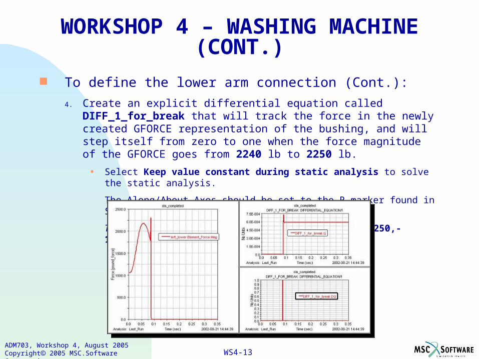
To define the lower arm connection (Cont.):

4. Create an explicit differential equation called DIFF_1_for_break that will track the force in the newly created GFORCE representation of the bushing, and will step itself from zero to one when the force magnitude of the GFORCE goes from 2240 lb to 2250 lb.

• Select Keep value constant during static analysis to solve the static analysis.

The Along/About Axes should be set to the R marker found in Step 3 .

Tip: STEP(GFORCE(left_lower,0,1,left_lower_body)-2250,-10.0,0,0.0,1)



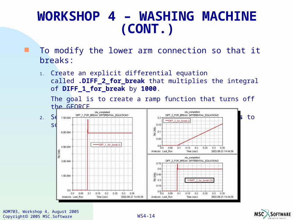
To modify the lower arm connection so that it breaks:

1. Create an explicit differential equation called .DIFF_2_for_break that multiplies the integral of DIFF_1_for_break by 1000.

The goal is to create a ramp function that turns off the GFORCE.

2. Select Keep value constant during static analysis to solve the static analysis.



To modify the lower arm connection so that it breaks (Cont.):

3. Modify the GFORCE created in Step 1 to turn off when DIFF_2_for_break becomes nonzero. In other words, use the ramp function to turn off the GFORCE, which represents the bushing breaking. For example,

FX = (-28000*DX(I,J,R)-10*VX(I,J,R))* step(dif(DIFF_2_for_break),0,1,0.001,0)

4. Similarly, apply a STEP function for the FY and FZ components.



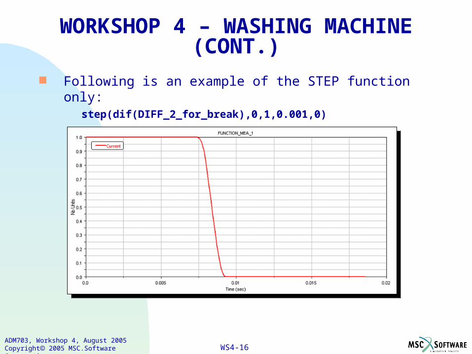
Following is an example of the STEP function only:step(dif(DIFF_2_for_break),0,1,0.001,0)



Simulating the enhanced model

1. Run a static equilibrium simulation.

2. Run a dynamic simulation for 0.35 seconds in 350 steps. You should see the connection break between the lower arm and the body.

3. At what time in the simulation does the lower arm-to-body connection break?

___________________________________________________________

4. In modeling this break, why was it necessary to scale DIFF_1_for_break by 1000, and then use that as the trigger for switching off the GFORCE?

___________________________________________________________

___________________________________________________________

5. What is the fundamental difference between this method of simulation-time model-topology manipulation and the method used in Workshop 6: Jet Engine Turbine? __________________________________________________________________

__________________________________________________________________



Analyzing with ADAMS/Linear

1. Perform a static simulation.

2. Perform a linear-modes analysis.

3. Review the mode shapes and natural frequencies using animation.

4. View the ADAMS/Linear results in tabular format and save the table to a file.

5. What are the undamped natural frequencies of modes 9 and 10? (Note: These might be slightly different, depending on modeling variations.)

_________________________________________________________________

What are the damping ratios of modes 9 and 10?

__________________________________________________________________

Do the motions of the system as expressed by the linear analysis seem to make sense given the model topology?

__________________________________________________________________

__________________________________________________________________


Documents

WS4-1 ADM703, Workshop 4, August 2005 Copyright 2005 MSC.Software Corporation WORKSHOP 4 WASHING MACHINE