www.monash.edu.au

Pre-processing for Data Mining

CSE5610 Intelligent Software SystemsSemester 1

www.monash.edu.au

2

Preprocessing

• Why preprocess the data?

• Data cleaning

• Data integration and transformation

• Data reduction

• Discretization and concept hierarchy generation

• Summary

www.monash.edu.au

3

Why Preprocessing?

• In reality data can be– incomplete: missing or wrong attribute values, or containing

only aggregate data

– noisy: may be due to errors or not appropriate values (known as outliers)

– inconsistent: containing discrepancies in codes or names

• Mining dirty data is not much useful (wrong inferences)!– Quality decisions must be based on quality data

– Data warehouse needs consistent integration of quality data

www.monash.edu.au

4

Measures to describe the Data Quality

• A well-accepted attributes are:– Accuracy– Completeness– Consistency– Timeliness– Believability– Value added– Interpretability– Accessibility

• Broad categories:– intrinsic, contextual, representational, and

accessibility.

www.monash.edu.au

5

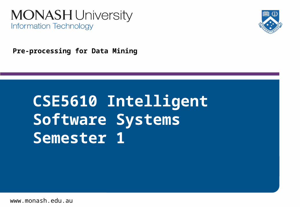
Major Tasks in Data Preprocessing

• Data cleaning– e.g. fill in missing values, smoothening noisy data, identify or

remove outliers, resolve inconsistencies• Data integration

– e.g: integration of data from multiple databases/sources, or files• Data transformation

– e.g: normalization and aggregation• Data reduction

– e.g: obtains reduced representation in volume but produces the same or similar analytical results

• Data discretization– e.g: part of data reduction but with particular importance,

especially for numerical data

www.monash.edu.au

6

Pictorially

www.monash.edu.au

7

Data Cleaning

• Data cleaning tasks

– Fill in missing values

– Identify outliers and smooth out noisy data

– Correct inconsistent data

www.monash.edu.au

8

Missing Data

• Data is not always available

– E.g., many tuples have no recorded value for several attributes

(for e.g. customer income in sales data)

• Missing data may be due to

– Data wasn’t capture due to equipment malfunction;

– inconsistent with other recorded data and thus application program might

have deleted the data;

– data not entered due to misunderstanding (I thought that you will do it!)

– certain data may not be considered important at the time of entry

– not register history or changes of the data

• Missing data values need to be inferred or estimated.

www.monash.edu.au

9

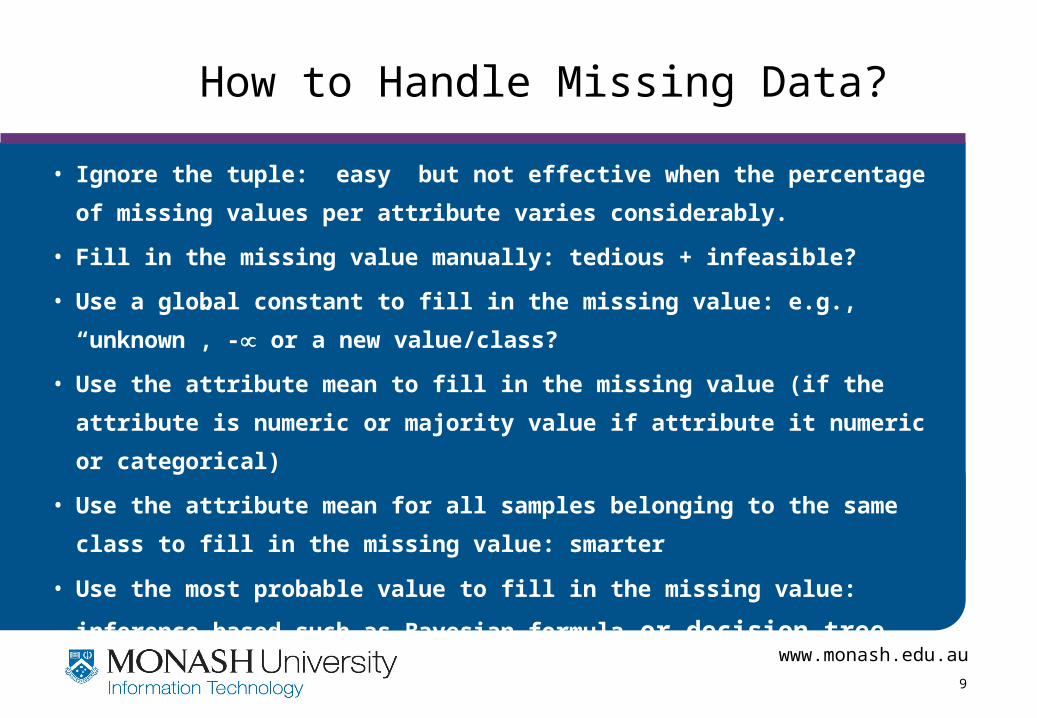
How to Handle Missing Data?

• Ignore the tuple: easy but not effective when the percentage of missing

values per attribute varies considerably.

• Fill in the missing value manually: tedious + infeasible?

• Use a global constant to fill in the missing value: e.g., “unknown”, - or a

new value/class?

• Use the attribute mean to fill in the missing value (if the attribute is

numeric or majority value if attribute it numeric or categorical)

• Use the attribute mean for all samples belonging to the same class to fill in

the missing value: smarter

• Use the most probable value to fill in the missing value: inference-based

such as Bayesian formula or decision tree.

www.monash.edu.au

10

Noisy Data

• Noise: random error or variance in a measured variable

• Noise can happen because of– faulty data collection instruments

– data entry mistakes

– data transmission problems

– inconsistency in naming convention

www.monash.edu.au

11

Correcting Noisy Data?

• Binning method:– first sort data and partition into (equi-depth or equal numbers) bins– then one can smooth by bin means, by bin median, by bin boundaries,

etc.

Let the data be { 4, 18, 15, 21,21,24,25,28,34}

Sort them into three (3 ) bins as {4,18,15}, {21,21,24} {25,28,34}

Smoothing by bin means: {9,9,9}, {22,22,22}, {29,29,29}

Smoothing by bin boundaries: {4,4,15}, {21,21,24}, {25,25,34}

What will be smooth by median?

www.monash.edu.au

12

Simple Binning- Formally

• Equal-width (distance) partitioning:– It divides the range into N intervals of equal size: uniform grid– if A and B are the lowest and highest values of the attribute, the

width of intervals will be: W = (B-A)/N.– The most straightforward– But outliers may dominate presentation– Skewed data is not handled well.

• Equal-depth (frequency) partitioning:– It divides the range into N intervals, each containing

approximately same number of samples– Good data scaling– Managing categorical attributes can be tricky.

www.monash.edu.au

13

Correcting Noisy Data?

• Clustering– detect and remove outliers

• Combined computer and human inspection– detect suspicious values and check by human

• Regression– smooth by fitting the data into regression

functions

www.monash.edu.au

14

Cluster Analysis

www.monash.edu.au

15

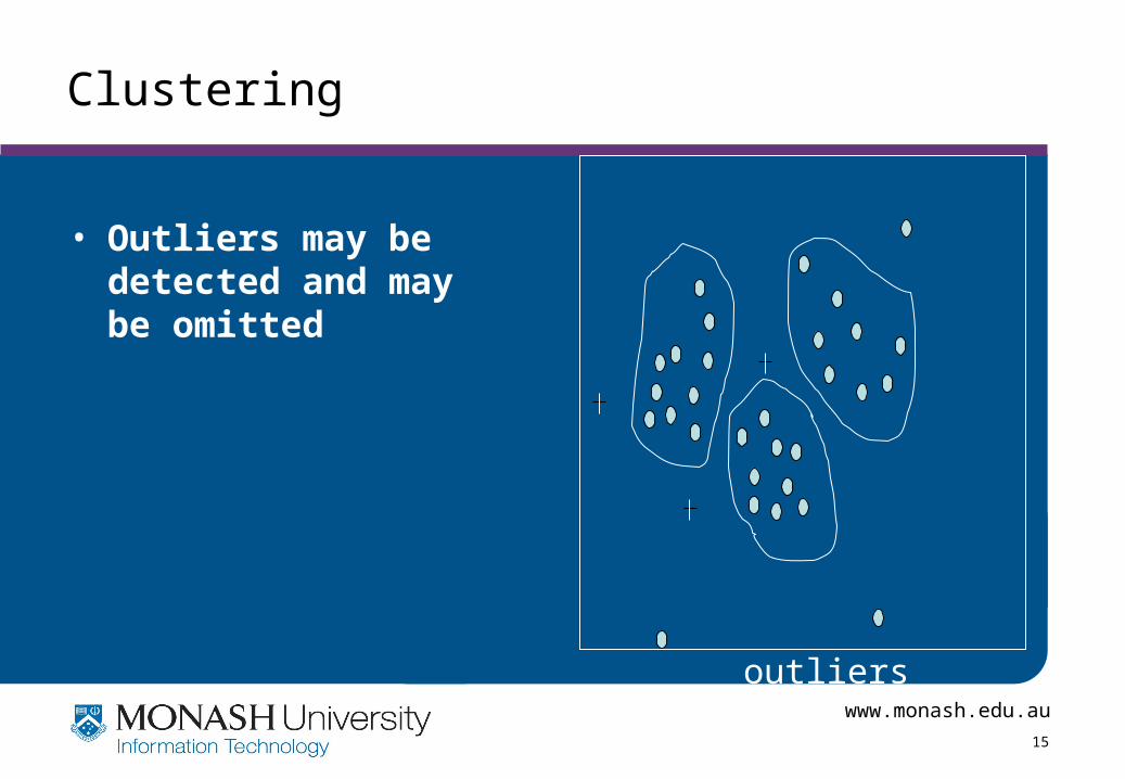
Clustering

• Outliers may be detected and may be omitted

outliers

www.monash.edu.au

16

Regression/Curve Fitting/Smoothing

x

y

y = x + 1

X1

Y1

Y1’

www.monash.edu.au

17

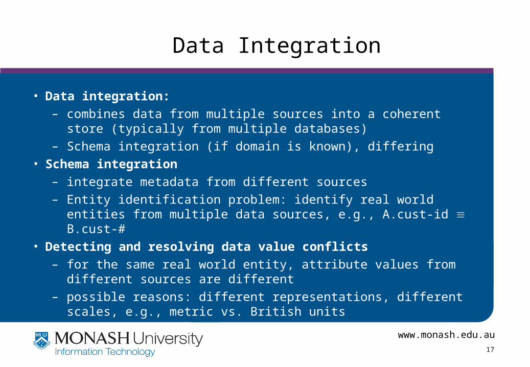
Data Integration

• Data integration:

– combines data from multiple sources into a coherent store (typically from multiple databases)

– Schema integration (if domain is known), differing

• Schema integration

– integrate metadata from different sources

– Entity identification problem: identify real world entities from multiple data sources, e.g., A.cust-id B.cust-#

• Detecting and resolving data value conflicts

– for the same real world entity, attribute values from different sources are different

– possible reasons: different representations, different scales, e.g., metric vs. British units

www.monash.edu.au

18

Handling Redundant Data in Data Integration

• Redundant data occur often when integration of multiple databases

– The same attribute may have different names in different databases

– One attribute may be a “derived” attribute in another table, e.g., annual revenue

• Redundant data may be able to be detected by correlational analysis

• Careful integration of the data from multiple sources may help reduce/avoid redundancies and inconsistencies and improve mining speed and quality

www.monash.edu.au

19

Data Transformation

• Smoothing: remove noise from data

• Aggregation: summarization, data cube construction

• Generalization: concept hierarchy climbing

• Normalization: scaled to fall within a small, specified range

– min-max normalization

– z-score normalization

– normalization by decimal scaling

• Attribute/feature construction

– New attributes constructed from the given ones

www.monash.edu.au

20

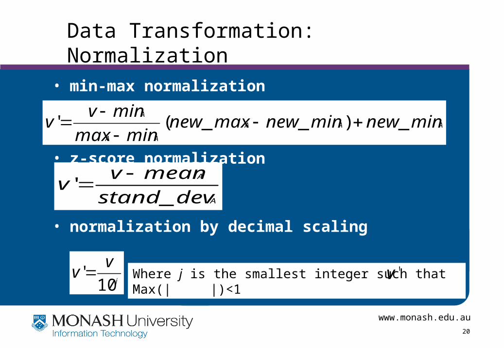
Data Transformation: Normalization

• min-max normalization

• z-score normalization

• normalization by decimal scaling

AAA

AA

A

minnewminnewmaxnewminmax

minvv _)__('

A

A

devstand

meanvv

_'

j

vv

10' Where j is the smallest integer such that Max(| |)<1'v

www.monash.edu.au

21

Data Reduction Strategies

• Database and data warehouse may store terabytes of data: Complex data analysis/mining may take a very long time to run on the complete data set – hence data reduction may be required for efficiency. – Obtains a reduced representation of the data set that is much

smaller in volume but yet produces the same (or almost the same) mining results (characteristics)

• Reduction strategies can be– (Data cube) aggregation

– Dimensionality reduction

– Numerosity reduction

– Discretization and concept hierarchy generation

www.monash.edu.au

22

Data Cube Aggregation

• The lowest level of a data cube

– the aggregated data for an individual entity of interest

– e.g., total sales for each year (from the monthly sales).

• Multiple levels of aggregation in data cubes

– e.g., total sales for each year per region.

• Reference appropriate levels

– Use the smallest representation which is enough to solve the task.

• Queries regarding aggregated information should be

answered using data cube, when possible.

www.monash.edu.au

23

Dimensionality Reduction

• Feature selection (i.e., attribute subset selection):– Select a minimum set of attributes such that the

probability distribution of different classes given the values for those attributes is as close as possible to the original distribution given the values of all features

– Reduction in size and easier to understand.• A number of heuristic methods (due to exponential

# of choices):– step-wise forward selection– step-wise backward elimination– combining forward selection and backward elimination– decision-tree induction

www.monash.edu.au

24

Example of Decision Tree Induction

Initial attribute set:{A1, A2, A3, A4, A5, A6}

A4 ?

A1? A6?

Class 1 Class 2 Class 1 Class 2

> Reduced attribute set: {A1, A4, A6}

www.monash.edu.au

26

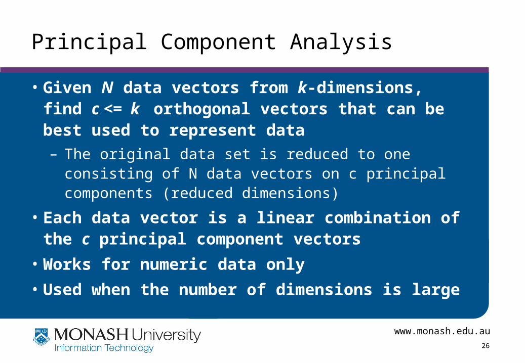
• Given N data vectors from k-dimensions, find c <= k orthogonal vectors that can be best used to represent data

– The original data set is reduced to one consisting of N data vectors on c principal components (reduced dimensions)

• Each data vector is a linear combination of the c principal component vectors

• Works for numeric data only

• Used when the number of dimensions is large

Principal Component Analysis

www.monash.edu.au

27

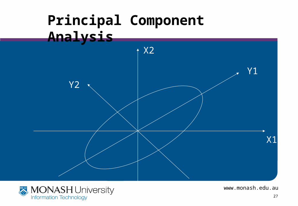
X1

X2

Y1

Y2

Principal Component Analysis

www.monash.edu.au

28

Histograms

• A popular data reduction technique

• Divide data into buckets and store average (sum) for each bucket

• Can be constructed optimally in one dimension using dynamic programming

• Related to quantization problems. 0

5

10

15

20

25

30

35

40

10000 30000 50000 70000 90000

www.monash.edu.au

29

Sampling

• Allow a mining algorithm to run in complexity that is potentially sub-linear to the size of the data

• Choose a representative subset of the data– Simple random sampling may have very poor performance in the

presence of skew

• Develop adaptive sampling methods– Stratified sampling:

> Approximate the percentage of each class (or subpopulation of interest) in the overall database

> Used in conjunction with skewed data• Sampling may not reduce database I/Os (page at a time).

www.monash.edu.au

30

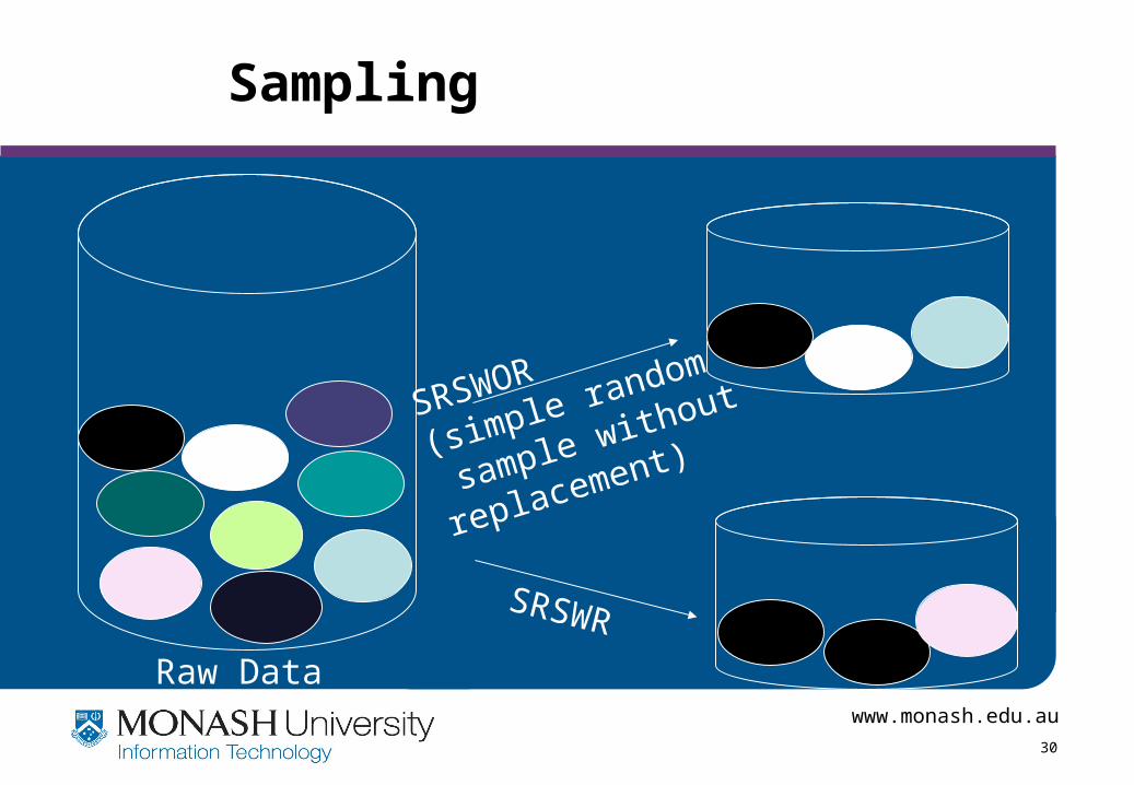
Sampling

SRSWOR

(simple random

sample without

replacement)

SRSWR

Raw Data

www.monash.edu.au

31

Sampling

Raw Data Cluster/Stratified Sample

www.monash.edu.au

32

Discretization

• Three types of attributes:– Nominal — values from an unordered set

– Ordinal — values from an ordered set

– Continuous — real numbers

• Discretization: divide the range of a continuous attribute into intervals

– Some classification algorithms only accept categorical attributes.

– Reduce data size by discretization

– Prepare for further analysis

www.monash.edu.au

33

Discretization and Concept hierachy

• Discretization

– reduce the number of values for a given continuous attribute by dividing the range of the attribute into intervals. Interval labels can then be used to replace actual data values.

• Concept hierarchies

– reduce the data by collecting and replacing low level concepts (such as numeric values for the attribute age) by higher level concepts (such as young, middle-aged, or senior).

www.monash.edu.au

34

Summary

• Data preparation is a major issue for both data

warehousing and data mining.

• Data preparation includes

– Data cleaning and data integration

– Data reduction and feature selection

– Discretization

• A number of methods exist, yet an active area of

research.