Embed Size (px)
Citation preview

XBeach skillbed report, revi-
sion 4664
status update trunk default
Revision: 4664
June 2, 2015

XBeach skillbed report, revision 4664
Published and printed by:
DeltaresRotterdamseweg 185p.o. box 1772600 MH DelftThe Netherlands
telephone: +31 88 335 85 85fax: +31 88 335 85 82e-mail: [email protected]: http://www.deltares.nl
For support contact:
telephone: +31 88 335 85 55fax: +31 88 335 81 11e-mail: [email protected]: http://www.xbeach.org/
Copyright © 2015 DeltaresAll rights reserved. No part of this document may be reproduced in any form by print,photo print, photo copy, microfilm or any other means, without written permission from thepublisher: Deltares.

XBeach skillbed report, revision 4664 Contents June 2015
4664
Contents
1 Introduction 1
1.1 Introduction to the XBeach model . . . . . . . . . . . . . . . . . . . . . . . . 1
1.2 Model approach and innovations . . . . . . . . . . . . . . . . . . . . . . . . . 2
1.3 XBeach skillbed . . . . . . . . . . . . . . . . . . . . . . . . . . . . . . . . . . . 3
2 Hydrodynamic tests 5
2.1 Long wave propagation . . . . . . . . . . . . . . . . . . . . . . . . . . . . . . . 5
2.2 1D wave runup (analytical solution) . . . . . . . . . . . . . . . . . . . . . . . 6
2.3 2D wave runup . . . . . . . . . . . . . . . . . . . . . . . . . . . . . . . . . . . 7
2.4 High- and low-frequency wave transformation . . . . . . . . . . . . . . . . . . 10
2.5 Field experiment: DELILAH . . . . . . . . . . . . . . . . . . . . . . . . . . . 11
2.6 Field experiment: Ningaloo reef . . . . . . . . . . . . . . . . . . . . . . . . . . 14
2.7 Longcrested refraction . . . . . . . . . . . . . . . . . . . . . . . . . . . . . . . 16
2.8 Tide . . . . . . . . . . . . . . . . . . . . . . . . . . . . . . . . . . . . . . . . . 19
2.8.1 Blankenberge . . . . . . . . . . . . . . . . . . . . . . . . . . . . . . . . 19
3 Morphological laboratory tests 21
3.1 Scale relations . . . . . . . . . . . . . . . . . . . . . . . . . . . . . . . . . . . . 21
3.1.1 Small scale tests . . . . . . . . . . . . . . . . . . . . . . . . . . . . . . 22
3.1.2 Additional small scale tests . . . . . . . . . . . . . . . . . . . . . . . . 24
3.1.3 Large scale tests . . . . . . . . . . . . . . . . . . . . . . . . . . . . . . 26
3.2 Large scale tests . . . . . . . . . . . . . . . . . . . . . . . . . . . . . . . . . . 33
3.2.1 Revetments . . . . . . . . . . . . . . . . . . . . . . . . . . . . . . . . . 33
3.2.2 Extreme conditions . . . . . . . . . . . . . . . . . . . . . . . . . . . . . 35
3.2.3 Bar evolution . . . . . . . . . . . . . . . . . . . . . . . . . . . . . . . . 38
3.2.4 Influence of wave period . . . . . . . . . . . . . . . . . . . . . . . . . . 40
Deltares iii

June 2015
4664
Contents XBeach skillbed report, revision 4664
4 Morphological field tests 59
4.1 1953 storm surge . . . . . . . . . . . . . . . . . . . . . . . . . . . . . . . . . . 59
4.2 1976 storm surge . . . . . . . . . . . . . . . . . . . . . . . . . . . . . . . . . . 60
4.3 Erosion and overwash of Asseteague Island . . . . . . . . . . . . . . . . . . . 62
4.4 Breach growth at Zwin . . . . . . . . . . . . . . . . . . . . . . . . . . . . . . . 63
4.5 MICORE field experiments . . . . . . . . . . . . . . . . . . . . . . . . . . . . 65
4.5.1 Lido di Dante, Italy . . . . . . . . . . . . . . . . . . . . . . . . . . . . 66
4.5.2 Praia de Faro, Portugal . . . . . . . . . . . . . . . . . . . . . . . . . . 67
4.5.3 Cadiz Urban Beach, Spain . . . . . . . . . . . . . . . . . . . . . . . . . 68
4.5.4 Dziwnow Spit, Poland . . . . . . . . . . . . . . . . . . . . . . . . . . . 69
4.5.5 Kamchia Shkorpilovtsi Beach, Bulgaria . . . . . . . . . . . . . . . . . 70
5 Comparisons with other models 73
5.1 Field applications . . . . . . . . . . . . . . . . . . . . . . . . . . . . . . . . . . 73
5.1.1 Retreat distances JARKUS . . . . . . . . . . . . . . . . . . . . . . . . 73
6 Specific functionalities 75
6.1 River outflow . . . . . . . . . . . . . . . . . . . . . . . . . . . . . . . . . . . . 75
6.2 Drifters . . . . . . . . . . . . . . . . . . . . . . . . . . . . . . . . . . . . . . . 76
6.3 Multiple sediment fractions . . . . . . . . . . . . . . . . . . . . . . . . . . . . 77
6.4 Curvilinear . . . . . . . . . . . . . . . . . . . . . . . . . . . . . . . . . . . . . 79
7 References 81
A Model Performance Statistics 87
A.1 Introduction . . . . . . . . . . . . . . . . . . . . . . . . . . . . . . . . . . . . . 87
A.2 MPS parameters . . . . . . . . . . . . . . . . . . . . . . . . . . . . . . . . . . 87
A.3 Mean Error & Standard Deviation . . . . . . . . . . . . . . . . . . . . . . . . 88
A.4 Correlation coefficient . . . . . . . . . . . . . . . . . . . . . . . . . . . . . . . 88
A.5 Relative Bias . . . . . . . . . . . . . . . . . . . . . . . . . . . . . . . . . . . . 88
A.6 Scatter Index . . . . . . . . . . . . . . . . . . . . . . . . . . . . . . . . . . . . 88
A.7 Brier Skill Score . . . . . . . . . . . . . . . . . . . . . . . . . . . . . . . . . . 88
A.8 Brier Skill Score (Murphy and Epstein, 1989) . . . . . . . . . . . . . . . . . . 89
B Overview 91
iv Deltares

XBeach skillbed report, revision 4664 Introduction June 2015
4664
Chapter 1
Introduction
1.1 Introduction to the XBeach model
The devastating effects of hurricanes on low-lying sandy coasts, especially during the 2004and 2005 seasons have pointed at an urgent need to be able to assess the vulnerabilityof coastal areas and (re-)design coastal protection for future events, and also to evaluatethe performance of existing coastal protection projects compared to ’do-nothing’ scenarios.In view of this the Morphos-3D project was initiated by USACE-ERDC, bringing togethermodels, modelers and data on hurricane winds, storm surges, wave generation and nearshoreprocesses. As part of this initiative an open-source program, XBeach for eXtreme Beachbehaviour, has been developed to model the nearshore response to hurricane impacts. Themodel includes wave breaking, surf and swash zone processes, dune erosion, overwashing andbreaching (Roelvink et al., 2009).
Existing tools to assess dune erosion under extreme storm conditions assume alongshoreuniform conditions and have been applied successfully along relatively undisturbed coasts(Vellinga, 1986; Steetzel, 1993; Nishi and Kraus, 1996; Larson et al., 2004), but are inadequateto assess the more complex situation where the coast has significant alongshore variability.This variability may result from anthropogenic causes, such as the presence of artificial inlets,sea walls, and revetments, but also from natural causes, such as the variation in dune heightalong the coast or the presence of rip channels and shoals on the shoreface (Thornton et al.,2007). A particularly complex situation is found when barrier islands protect storm impact onthe main land coast. In that case the elevation, width and length of the barrier island, as wellas the hydrodynamic conditions (surge level) of the back bay should be taken into accountto assess the coastal response. Therefore, the assessment of storm impact in these morecomplex situations requires a two-dimensional process-based prediction tool, which containsthe essential physics of dune erosion and overwash, avalanching, swash motions, infragravitywaves and wave groups.
With regard to dune erosion, the development of a scarp andepisodic slumping after under-cutting is a dominant process (Van Gent et al., 2008). This supplies sand to the swash andsurf zone that is transported seaward by the backwash motion and by the undertow; withoutit the upper beach scours down and the dune erosion process slows down considerably. One-dimensional (cross-shore) models such as DUROSTA (Steetzel, 1993) focus on the underwateroffshore transport and obtain the supply of sand by extrapolating these transports to the drydune. Overton and Fisher (1988), Nishi and Kraus (1996) focus on the supply of sand by thedune based on the concept of wave impact. Both approaches rely on heuristic estimates of
Deltares 1

June 2015
4664
Introduction XBeach skillbed report, revision 4664
the runup and are well suited for 1D application but difficult to apply in a horizontally 2Dsetting. Hence, a more comprehensive modelling of the swash motions is called for.
Swash motions are up to a large degree a result from wave-group forcing of infragravitywaves (Tucker, 1954). Depending on the beach configuration and directional properties ofthe incident wave spectrum both leaky and trapped infragravity waves contribute to the swashspectrum (Huntley et al., 1981). Raubenheimer and Guza (1996) show that incident bandswash is saturated, infragravity swash is not, therefore infragravity swash is dominant in stormconditions. Models range from empirical formulations (e.g. Stockdon et al., 2006) throughanalytical approaches (Schaeffer, 1994; Erikson et al., 2005) to numerical models in 1D (e.g.List, 1992; Roelvink, 1993b) and 2DH (e.g. Van Dongeren et al., 2003; Reniers et al., 2004a,2006). 2DH wavegroup resolving models are well capable of describing low-frequency motions.However, for such a model to be applied for swash, a robust drying/flooding formulation isrequired.
1.2 Model approach and innovations
Our aim is to model processes in different regimes as described by Sallenger (2000). He definesan Impact Level to denote different regimes of impact on barrier islands by hurricanes, whichare the 1) swash regime, 2) collision regime, 3) overwash regime and 4) inundation regime.The approach we follow to model the processes in these regimes is described below.
To resolve the swash dynamics the model employs a novel 2DH description of the wave groupsand accompanying infragravity waves over an arbitrary bathymetry (thus including bound,free and refractively trapped infragravity waves). The wave-group forcing is derived fromthe time-varying wave-action balance (e.g. Phillips, 1977) with a dissipation model for usein combination with wave groups (Roelvink, 1993a). A roller model (Svendsen, 1984; Nairnet al., 1990; Stive and De Vriend, 1994) is used to represent momentum stored in surfacerollers which leads to a shoreward shift in wave forcing.
The wave-group forcing drives infragravity motions and both longshore and cross-shore cur-rents. Wave-current interaction within the wave boundary layer results in an increased wave-averaged bed shear stress acting on the infragravity waves and currents (e.g. Soulsby et al.,1993, and references therein). To account for the randomness of the incident waves the de-scription by Feddersen et al. (2000) is applied which showed good skill for longshore currentpredictions using a constant drag coefficient (Ruessink et al., 2001).
During the swash and collision regime the mass flux carried by the waves and rollers returnsoffshore as a return flow or a rip-current. These offshore directed flows keep the erosionprocess going by removing sand from the slumping dune face. Various models have beenproposed for the vertical profile of these currents (see Reniers et al., 2004b, for a review).However, the vertical variation is not very strong during extreme conditions and has beenneglected for the moment.
Surf and swash zone sediment transport processes are very complex, with sediment stirring bya combination of short-wave and long-wave orbital motion, currents and breaker-induced tur-bulence. However, intra-wave sediment transports due to wave asymmetry and wave skewnessare expected to be relatively minor compared to long-wave and mean current contributions(Van Thiel de Vries et al., 2008). This allows for a relatively simple and transparent formula-tion according to Soulsby & Van Rijn (Soulsby, 1997) in a shortwave averaged but wave-groupresolving model of surf zone processes. This formulation has been applied successfully in de-scribing the generation of rip channels (Damgaard et al., 2002; Reniers et al., 2004a) and
2 Deltares

XBeach skillbed report, revision 4664 Introduction June 2015
4664
barrier breaching (Roelvink et al., 2003).
In the collision regime, the transport of sediment from the dry dune face to the wet swash, i.e.slumping or avalanching, is modeled with an avalanching model accounting for the fact thatsaturated sand moves more easily than dry sand, by introducing both a critical wet slope anddry slope. As a result slumping is predominantly triggered by a combination of infragravityswash runup on the previously dry dune face and the (smaller) critical wet slope.
During the overwash regime the flow is dominated by lowfrequency motions on the time scaleof wave groups, carrying water over the dunes. This onshore flux of water is an importantlandward transport process where dune sand is being deposited on the island and withinthe shallow inshore bay as overwash fans (e.g. Leatherman et al., 1977; Wang and Horwitz,2007). To account for this landward transport some heuristic approaches exist in 1D, e.g. inthe SBeach overwash module (Larson et al., 2004) which cannot be readily applied in 2D.Here, the overwash morphodynamics are taken into account with the wave-group forcing oflow-frequency motions in combination with a robust momentum-conserving drying/floodingformulation (Stelling and Duinmeijer, 2003) and concurrent sediment transport and bed-elevation changes.
Breaching of barrier islands occurs during the inundation regime, where a new channel isformed cutting through the island. Visser (1998) presents a semi-empirical approach forbreach evolution based on a schematic uniform cross-section. Here a generic description isused where the evolution of the channel is calculated from the sediment transports inducedby the dynamic channel flow in combination with avalanche-triggered bank erosion.
1.3 XBeach skillbed
The XBeach code and related functionalities develop fast. As a result there is a need frommodelers and code developers to develop a tool that gives insight in the effect of code devel-opments on model performnace. The XBeach skillbed tries to fulfill this need by running arange of tests including analytical solutions, laboratory tests and practical field cases everyweek with the latest code.
Deltares 3

June 2015
4664
Introduction XBeach skillbed report, revision 4664
4 Deltares
XBeach skillbed report, revision 4664 Hydrodynamic tests June 2015
4664
Chapter 2
Hydrodynamic tests
Morphodynamics start with hydrodynamics. In this chapter the hydrodynamic results ofXBeach are discussed. All tests are run without the morphological module and the analsyisis focussed on the wave propagation and transformation computed by XBeach.
First, two analytical solutions are reproduced by XBeach. Subsequently, two laboratoryexperiments are discussed and finally a field experiment.
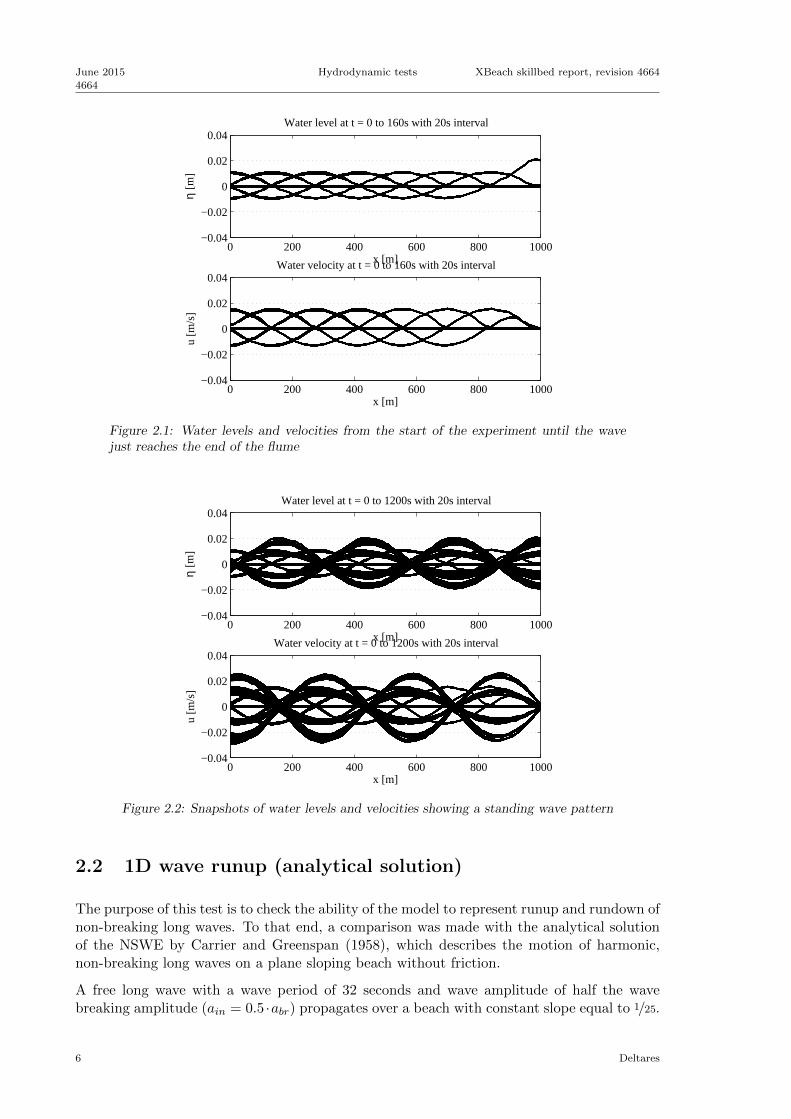
2.1 Long wave propagation
The purpose of the this test is to check if the NSWE numerical scheme is not too dissipativeand that it does not create large errors in propagation speed.
A long wave with a small amplitude of 0.01m and period of 80s was sent into a domain of5m depth, grid size of 5m and a length of 1km. At the end, a fully reflecting wall is imposed.The wave length in this case should be
√g · d · T =
√9.81 · 5 · 80 = 560m. The velocity
amplitude should be√g/h ·A =
√9.81/5 ·0.01 = 0.014m. After the wave has reached the wall,
a standing wave with double amplitude should be created.
Deltares 5
June 2015
4664
Hydrodynamic tests XBeach skillbed report, revision 4664
0 200 400 600 800 1000−0.04
−0.02
0
0.02
0.04Water level at t = 0 to 160s with 20s interval
x [m]
η [m
]
0 200 400 600 800 1000−0.04
−0.02
0
0.02
0.04Water velocity at t = 0 to 160s with 20s interval
x [m]
u [m
/s]
Figure 2.1: Water levels and velocities from the start of the experiment until the wavejust reaches the end of the flume
0 200 400 600 800 1000−0.04
−0.02
0
0.02
0.04Water level at t = 0 to 1200s with 20s interval
x [m]
η [m
]
0 200 400 600 800 1000−0.04
−0.02
0
0.02
0.04Water velocity at t = 0 to 1200s with 20s interval
x [m]
u [m
/s]
Figure 2.2: Snapshots of water levels and velocities showing a standing wave pattern
2.2 1D wave runup (analytical solution)
The purpose of this test is to check the ability of the model to represent runup and rundown ofnon-breaking long waves. To that end, a comparison was made with the analytical solutionof the NSWE by Carrier and Greenspan (1958), which describes the motion of harmonic,non-breaking long waves on a plane sloping beach without friction.
A free long wave with a wave period of 32 seconds and wave amplitude of half the wavebreaking amplitude (ain = 0.5 ·abr) propagates over a beach with constant slope equal to 1/25.
6 Deltares

XBeach skillbed report, revision 4664 Hydrodynamic tests June 2015
4664
The wave breaking amplitude is computed as abr = 1/√
128·π3 ·s2.5 ·T 2.5 ·g1.25 ·h−0.250 = 0.0307m,
where s is the beach slope, T is the wave period and h0 is the still water depth at the seawardboundary. The grid is non uniform and consists of 160 grid points. The grid size ∆x isdecreasing in shoreward direction and is proportional to the (free) long wave celerity (
√g · h).
The minimum grid size in shallow water was set at ∆x = 0.1m.
To compare XBeach output to the analytical solution of Carrier and Greenspan (1958), thefirst are non-dimensionalized with the beach slope s, the acceleration of gravity g, the waveperiod T , a horizontal length scale Lx and the vertical excursion of the swash motion A. Thehorizontal length scale Lx is related to the wave period via T =
√Lx/g·s and the vertical
excursion of the swash motion A is expressed as: A = ain · π/√
0.125·s·T ·√g/h0
50 60 70 80 90 100 110 120 130 140 150
4.8
4.9
5
5.1
5.2
cross−shore distance [m]
wat
er le
vel [
m]
Water level variation in time
50 60 70 80 90 100 110 120 130 140 150
−1
−0.5
0
0.5
1
cross−shore distance [m]
flow
vel
ocity
[m/s
]
Water velocity variation in time
Figure 2.3: Snapshots of water level and velocity
2.3 2D wave runup
The verification cases so far considered solely the cross-shore dimension and assumed a long-shore uniform coast. In the following case the potential of the model to predict coastal anddune erosion in situations that include the two horizontal dimensions is further examined.A first step towards a 2DH response is to verify that the 2DH forcing by surge run-up andrun-down is accurately modelled by testing not against Zelt (1986), but actually Ozkan-Hallerand Kirby (1997). The reason is that Zelt modeled the NSW equations including some dis-persive and dissipative terms, which the present model does not include. For that reason, wecompared the model to the results of Ozkan-Haller and Kirby (1997) who modeled the NSWequations using a Fourier-Chebyshev Collocation method, which does not have any numericaldissipation or dispersion errors. They use a moving, adapting grid with a fixed ∆y (whichis equal to the present model’s ∆y in this comparison) but with a spatially and temporallyvarying ∆x so that the grid spacing in x near the shoreline is very small. In the presentmodel ∆x is set equal to ∆y, which means that we can expect to have less resolution at theshoreline than Ozkan-Haller and Kirby (1997).
Deltares 7

June 2015
4664
Hydrodynamic tests XBeach skillbed report, revision 4664
Figure 2.4: Definition scetch of concave beach bathymetry
Figure 2.4 shows the definition sketch of the concave beach bathymetry in the present coor-dinate system, converted from the original system by Zelt (1986). The bathymetry consistsof a flat bottom part and a beach part with a sinusoidally varying slope. For Zelt (1986)’sfixed parameter choice of
√β = hs
Ly= 4
10π , the bathymetry is given by
h = {
hs , x ≤ Lshs − 0.4(x−Ls)
3−cos(πyLy
) , x > Ls
where hs is the shelf depth, Ls is the length of the shelf in the modeled domain and Ly isthe length scale of the longshore variation of the beach. This results in a beach slope ofhx = 1
10 in the center of the bay and of hx = 15 normal to the “headlands”. In the following
we chose Ly = 8m, which determines hs = 1.0182m. We set Ls = Ly. Different values forLs only cause phase shifts in the results, but no qualitative difference, so this parameter isnot important in this problem. Also indicated in the figure are the five stations where thevertical run-up (the surface elevation at the shoreline) will be measured.
At the offshore (x = 0) boundary we specify an incoming solitary wave, which in dimensionalform reads
ζi(t) = αhssech2(√
3g4hs
α(1 + α)(t− to))
8 Deltares

XBeach skillbed report, revision 4664 Hydrodynamic tests June 2015
4664
which is similar to Zelt (1986)’s Eq. (5.3.7). The phase shift to is chosen such that the surfaceelevation of the solitary wave at t = 0 is 1% of the maximum amplitude. The only parameteryet to be chosen is α. We will compare our model to Zelt’s case of α = H
hs= 0.02, where
H is the offshore wave height. Zelt found that the wave broke for a value of α = 0.03, sothe present test should involve no breaking, but has a large enough nonlinearity to exhibit apronounced two-dimensional run-up.
Any outgoing waves will be absorbed at the offshore boundary by the absorbing-generatingboundary condition. At the lateral boundaries y = 0 and y = 2Ly we specify a no-flux(wall) boundary condition following Zelt (1986). The model equations used in this test arethe nonlinear shallow water equations without forcing or friction. The numerical parametersare ∆x = ∆y = 1
8 m with a Courant number ν = 0.7.
−5 0 5 10 15−5
0
0
0
0
0
5
t/T
ζ/H
0 0.5 1 1.5 2−6
−4
−2
0
2
4
6
y/Ly
ζ/H
Figure 2.5: Normalized vertical runup in time (panel 1) and maximum and minimumvalues (panel 2)
The first panel in Figure 2.5 shows the vertical runup normalized with the offshore wave heightH as a function of time, which is normalized by
√g hs/Ly at the 5 cross-sections indicated in
Figure 2.4. The solid lines represent the present model results, while the dashed lines denotesOzkan-Haller and Kirby (1997)’s numerical results. The second panel in Figure 2.5 shows themaximum vertical run-up and run-down, normalized by H, versus the alongshore coordinatey. Table 2.1 presents error statistics of the model run with respect to the measurements.
Table 2.1
R2 Sci Rel. bias BSS
Timeseries (min) 0.10 0.23 -0.15 -5.14Timeseries (max) 0.97 2.27 0.09 0.94Max. runup 0.99 0.09 -0.09 0.99
Deltares 9

June 2015
4664
Hydrodynamic tests XBeach skillbed report, revision 4664
2.4 High- and low-frequency wave transformation
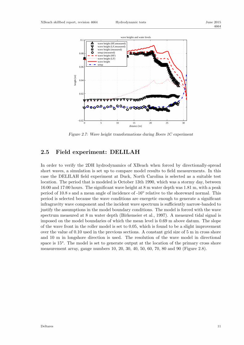
Boers (1996) performed experiments with irregular waves in the physical wave flume at DelftUniversity of Technology with a length of 40 meters and a width of 0.8 m. The flume isequipped with a hydraulically driven, piston type wave generator with second-order wavegeneration and Active Reflection Compensation. Boers ran waves over a concrete bar-troughbeach, which was modelled after the Delta Flume experiments. He ran three different irregularwave conditions, but in this report we will focus on case 1C, a Jonswap spectrum with Hm,0 =0.1m and Tp = 3.3s. The surface elevation was measured in 70 locations shown in Figure 2.6.
Figure 2.6: Locations of surface eleveation measurements
The comparison between the model and the data for the wave height transformation of theshort waves and the long waves (defined as waves with a frequency greater than fp/2 and lessthan fp/2, respectively) is shown in Figure 2.7.
The red dashed line and triangles indicate the short wave height transformation. The blueline and circles indicate the mean (steady) set-up. The dotted red line and upside-downtraiangles indicate the total (incoming and reflected) low frequency wave.
The observational data is separated into incoming and reflected long wave components usingan array of wave gauges (Bakkenes, 2002) and the numerical data has been separated intotwo components using co-located surface elevation and velocity information.
10 Deltares
XBeach skillbed report, revision 4664 Hydrodynamic tests June 2015
4664
0 5 10 15 20 25 30−0.02
0
0.02
0.04
0.06
0.08
0.1wave heights and water levels
heig
ht [m
]
distance [m]
wave height (HF,measured)wave height (LF,measured)wave height (measured)setup (measured)wave height (HF)wave height (LF)wave heightsetup
Figure 2.7: Wave height transformations during Boers 1C experiment
2.5 Field experiment: DELILAH
In order to verify the 2DH hydrodynamics of XBeach when forced by directionally-spreadshort waves, a simulation is set up to compare model results to field measurements. In thiscase the DELILAH field experiment at Duck, North Carolina is selected as a suitable testlocation. The period that is modeled is October 13th 1990, which was a stormy day, between16:00 and 17:00 hours. The significant wave height at 8 m water depth was 1.81 m, with a peakperiod of 10.8 s and a mean angle of incidence of -16o relative to the shoreward normal. Thisperiod is selected because the wave conditions are energetic enough to generate a significantinfragravity wave component and the incident wave spectrum is sufficiently narrow-banded tojustify the assumptions in the model boundary conditions. The model is forced with the wavespectrum measured at 8 m water depth (Birkemeier et al., 1997). A measured tidal signal isimposed on the model boundaries of which the mean level is 0.69 m above datum. The slopeof the wave front in the roller model is set to 0.05, which is found to be a slight improvementover the value of 0.10 used in the previous sections. A constant grid size of 5 m in cross shoreand 10 m in longshore direction is used. The resolution of the wave model in directionalspace is 15o. The model is set to generate output at the location of the primary cross shoremeasurement array, gauge numbers 10, 20, 30, 40, 50, 60, 70, 80 and 90 (Figure 2.8).
Deltares 11

June 2015
4664
Hydrodynamic tests XBeach skillbed report, revision 4664
Figure 2.8: Bathymetry and measurement locations
The modeled time-averaged wave heights of the short waves are compared to the time-averaged wave heights measured at the gauges. These results are shown in the first panel ofFigure 2.9. Unfortunately, no data exist for gauge number 60.
The infragravity wave height is calculated as follows (Van Dongeren et al., 2003):
Hrms,low =√
8∫ 0.05Hz
0.005Hz Sdf
Figure 2.9 shows the infragravity wave height. The measured and modelled time-averagedlongshore current are shown in the second panel of Figure 2.9. The correlation coefficient,scatter index, relative bias and Brier Skill Score for the simulation are shown in Table 2.2.
12 Deltares

XBeach skillbed report, revision 4664 Hydrodynamic tests June 2015
4664
0 100 200 300 400 500 600 700 800 9000
0.5
1
1.5
2wave heights and water levels
heig
ht [m
]distance [m]
wave height (HF,measured)wave height (LF,measured)wave height (measured)wave height (HF)wave height (LF)wave height
0 100 200 300 400 500 600 700 800 900−1.5
−1
−0.5
0flow velocities
velo
city
[m/s
]
distance [m]
flow velocity (v,mean,measured)flow velocity (v,mean)
Figure 2.9: Wave height transformation and flow velocities during the DELILAH fieldexperiment 1990
Table 2.2
R2 Sci Rel. bias BSS
Hrmslf 0.70 0.13 -0.12 0.50Hrmshf 0.94 0.15 -0.12 0.76vmean 0.69 0.46 0.28 0.43
The modeled and measured sea surface elevation spectra at four gauge locations are shownin Figure 2.10. Note that the modeled surface elevation spectra only contain low frequencycomponents associated with wave groups.
Deltares 13

June 2015
4664
Hydrodynamic tests XBeach skillbed report, revision 4664
0 0.1 0.2 0.30
0.1
0.2
0.3
0.41
f [Hz]
S ηη [
m2 /H
z]
0 0.1 0.2 0.30
0.2
0.4
0.6
0.82
f [Hz]
S ηη [
m2 /H
z]
0 0.1 0.2 0.30
0.1
0.2
0.3
0.4
0.53
f [Hz]
S ηη [
m2 /H
z]
0 0.1 0.2 0.30
0.2
0.4
0.6
0.84
f [Hz]
S ηη [
m2 /H
z]
Figure 2.10: Modelled surface elevation spectra for four locations in the primary crossshore array during the DELILAH field experiment 1990
2.6 Field experiment: Ningaloo reef
Ningaloo Reef is a large fringing reef on the northwest coast of Australia and consists of aseries of reef-channel cells, exposed to tropical cyclones and Southern Ocean swells. A fielddata set of wave transformation on a shore-normal transect (Figure 2.11) taken at Sandy Bayin June 2009 is described in (Pomeroy et al., 2012). The transect is composed of a steep forereef, a shallow reef flat ( 1− 2m depth) that is separated from the shore by a slightly deeperlagoon ( 2− 3m average depth). Instrument C1 was deployed on the forereef slope, C3 andC4 were located on the reef flat, while C5 and C6 were located inside the lagoon behind thereef. The wave field exhibits a dramatic decay in the incident swell band on the fore reefsection with a transfer of part of the energy to infragravity waves which are dissipated dueto bottom friction over the reef flat and lagoon.
The XBeach model formulations have been extended with a friction dissipation term in thewave action equation (Dongeren et al. (2013), which also describes the following case). Forthis site, optimum friction coefficient values (fw = 0.6, cf = 0.1) were determined for a 1Dversion of the model based on conditions at the peak of the swell event. These settings weresubsequently used to simulate the entire swell event from June 14 12:00 hours to June 1900:00 hours (109 hours in total) when wave conditions varied significantly. Good agreementwas generally observed throughout the simulation and at all sites (??; Figure 5 in Dongerenet al. (2013)). The model reproduced the spatial variability in wave heights across the reef,as well as temporal changes in the response to the varying offshore wave conditions and tidalvariations. The short wave height predictions matched the data reasonably well (?? a-e),except for a small positive bias of a few centimeters. The IG wave heights were slightlyunder predicted (negative bias) at C1, but were generally in very good agreement for siteson the reef (?? f-j). The time series of the predicted mean water level residuals (the time-averaged difference between the observed water level on the reef and the observation at C1,∆zs = zs − zs,C1, thus describing wave setup) followed the observed residuals reasonably well,albeit that the model over predicts the observations by about 0.1 m. (?? l-o) Note that at
14 Deltares

XBeach skillbed report, revision 4664 Hydrodynamic tests June 2015
4664
C1 the observed and predicted water levels rather than the residuals are shown (?? k). Asummary of the model skill (bias and the RMS error) for the short wave heights, IG heightsand mean water level is shown in ?? (Figure 6 in Dongeren et al. (2013)).
Figure 2.11: Cross-shore profile of the bathymetry along the main measurement transectwith instrument locations shown.
06/1506/1606/1706/1806/190
2
4(a)
Hrms.sw
(m)
06/1506/1606/1706/1806/190
0.2
0.4(b)
06/1506/1606/1706/1806/190
0.1
0.2(c)
06/1506/1606/1706/1806/190
0.1
0.2(d)
06/1506/1606/1706/1806/190
0.1
0.2(e)
06/1506/1606/1706/1806/190
0.10.30.5
(f)
Hrms.IG
(m)
06/1506/1606/1706/1806/190
0.10.30.5
(g)
06/1506/1606/1706/1806/190
0.10.30.5
(h)
06/1506/1606/1706/1806/190
0.10.30.5
(i)
06/1506/1606/1706/1806/190
0.10.30.5
(j)
06/1506/1606/1706/1806/19−1
0
1(k)
zs (m)
06/1506/1606/1706/1806/19−1
0
1(l)
06/1506/1606/1706/1806/19−1
0
1(m)
06/1506/1606/1706/1806/19−1
0
1(n)
06/1506/1606/1706/1806/19−1
0
1(o)
Figure 2.12: Comparison between the 1D model results (blue) and measured data (red)for the duration of the 5 day swell event. (a,f,k) are for instrument C1, (b,g.l) C3, (c,h,m)C4, (d,i,n) C5 and (e,j,o) C6. The peak of the storm is indicated by the red vertical line.Note the large reduction in vertical scale between C1 and the reef sites C3-C6.
Deltares 15

June 2015
4664
Hydrodynamic tests XBeach skillbed report, revision 4664
C1 C3 C4 C5 C6−0.15
−0.1
−0.05
0
0.05
0.1
0.15
Instruments
Bia
s (m
)
(a)
C1 C3 C4 C5 C60
0.05
0.1
0.15
Instruments
RM
SE
(m
)
(b)
SwellIGz
s
Figure 2.13: Bias and RMS error from the 1D swell duration ( 5 day) model resultscompared with the measured data at each site, based on the short wave heights, IG waveheights, and mean water levels.
2.7 Longcrested refraction
Longcrested waves are supported in XBeach by using a value s larger than 1,000. Thedirectional distribution in that case is a spike corresponding to the mean wave direction. Dueto the discretization in the wave directional dimension, numerical diffusion in this dimensionmay occur. In case of a narrow directional distribution, the numerical diffusion may lead toa loss of wave energy through the boundaries of the directional grid.
To limit the numerical directional diffusion, the directional grid may be chosen with large gridcells and thus decreasing the gradients between adjacent grid cells. Directional advection maybe turned of entirely when using a single directional grid cell, since refraction is not possiblewith a single grid cell at all. However, when using oblique longcrested waves in a 2DH model,none of these solutions suffice.
This test shows the numerical directional diffusion in the comparison of a few runs where theangle of wave incidence and the number of directional bins vary. The bathymetry is a linearsloping beach and no morphological change is computed in these runs.
0o
1 bi
n
0 0.5 10
0.5
110o
0 0.5 10
0.5
120o
3 bi
n5
bin
Figure 2.14: Wave height
16 Deltares

XBeach skillbed report, revision 4664 Hydrodynamic tests June 2015
4664
0o
1 bi
n
0 0.5 10
0.5
110o
0 0.5 10
0.5
120o
3 bi
n5
bin
Figure 2.15: Mean wave direction
0o
1 bi
n
0 0.5 10
0.5
110o
0 0.5 10
0.5
120o
3 bi
n5
bin
Figure 2.16: Time-averaged wave forcing in lateral direction
This test is to check the refraction behaviour of loncrested waves, which are simulated usinginstat=stat and m=1000. Four cases are generated and compared: directional bins of 2.5, 5and 10 degrees and a single bin. In all cases the incident wave angle is 60 degrees and thetagrid runs from -10 to 90 degrees. The results are compared among themselves and, for thewave direction, with Snel’s law and with mean direction computed by integrating cθ/cg,x overx. The results all agree within approx. one degree, whch is considered satisfactory. Notethat the longshore current does not exhibit any negative velocities, as was noticed when therefraction is not computed correctly.
Deltares 17

June 2015
4664
Hydrodynamic tests XBeach skillbed report, revision 4664
0 100 200 300 400 500 600 700 800 900 1000−20
−10
0
bath
ymet
ry [m
]
0 100 200 300 400 500 600 700 800 900 1000200
250di
rect
ion
[o ]
0 100 200 300 400 500 600 700 800 900 10000
2
H [m
]
0 100 200 300 400 500 600 700 800 900 1000−0.2
0
0.2
ue [m
]
0 100 200 300 400 500 600 700 800 900 1000
0
1
2
ve [m
]
distance [m]
10o
2p5o
5o
snellius
Figure 2.17: Wave energy, direction and flow velocities for different sized of theta bins.
0 20 40 60 80
0
200
400
600
800
1000
dist
ance
[m
]
10o
0
5000
10000
15000
0 20 40 60 80
0
200
400
600
800
10002p5o
0
5000
10000
15000
0 20 40 60 80
0
200
400
600
800
1000
direction [o]
dist
ance
[m
]
5o
0
5000
10000
15000
0 20 40 60 80
0
200
400
600
800
1000
direction [o]
snellius
0
5000
10000
15000
Figure 2.18: Refraction with different sizes of theta bins. The red dotted line indicatesthe solution according to Snel law.
18 Deltares

XBeach skillbed report, revision 4664 Hydrodynamic tests June 2015
4664
2.8 Tide
This test was set up to verify the capability of XBeach to model tidal elevation and longshorecurrents in a small model, based on water level time series at the seaward corner points,which have a small time shift. The current pattern should spin up in a longshore uniformpattern and remain longshore uniform at all times. In the figure velocity patterns at sixtimes during a one-day simulation are shown. Also the input timeseries of water levels at thecorners (dots) can be compared with the model water
level time series, which should closely follow the input but may have a small delay dependingon the type of boundary condition chosen (abs 1d, abs 2d or waterlevel) and on settings ofepsi (-1 in this case) and cats (5). In this case without wave forcing, the abs 2d boundarytype does not perform well; water levels do not match the input. This is probably due to theabsence of waves. With abs 1d the results as in the reference figure are shown.
0 5 10 15 20
2
4
6
time [hr]
zs [m
]
−1000
−500
0
500
t = 12hr
y [m
]
t = 14hr t = 16hr
0 1000 2000
−1000
−500
0
500
t = 18hr
y [m
]
x [m]0 1000 2000
t = 20hr
x [m]0 1000 2000
t = 22hr
x [m]
velocity [m/s] 0
0.1
0.2
0.3
0.4
Figure 2.19: The lower-left panel shows the tidal timeseries imposed to the offshore cornersof the model (dots) and the generated waterlevels at these locations (lines). For sixmoments indicated with the black vertical lines, the flow field is shown in the upperpanels.
2.8.1 Blankenberge
This represents a realistic test model of the coast and port of Blankenberge on the Belgiancoast, in a model set up by IMDC and Flanders Hydraulics. The model experienced badtidal currents; after fixing this problem the accompanying figure show smooth and realisticcurrent patterns with a nearshore current dominated by wave-driven currents (instationary,JONSWAP-type, with waves from 270 degrees, so a large angle to the coast. In this case theabs 2d boundary option does not pose a problem to the tidal forcing. In the present setupwe run it with theta bins of 20 degrees.
Deltares 19

June 2015
4664
Hydrodynamic tests XBeach skillbed report, revision 4664
0 5 10 15 20
−1
0
1
time [hr]
zs [m
]3.71
3.72
3.73
3.74
x 105 t = 6hr
y [m
]
t = 8hr t = 10hr
−6000 −4000 −2000
3.71
3.72
3.73
3.74
x 105 t = 12hr
y [m
]
x [m]−6000 −4000 −2000
t = 14hr
x [m]−6000 −4000 −2000
t = 16hr
x [m]
velocity [m/s] 0
0.5
1
Figure 2.20: The lower-left panel shows the tidal timeseries imposed to the offshore cornersof the model (dots) and the generated waterlevels at these locations (lines). For sixmoments indicated with the black vertical lines, the flow field is shown in the upperpanels.
20 Deltares

XBeach skillbed report, revision 4664 Morphological laboratory tests June 2015
4664
Chapter 3
Morphological laboratory tests
In this chapter, the performance of XBeach is compared to results obtained from physicalmodel tests performed in a variety of laboratory facilities. Many of those tests are part offundamental research into dune erosion and other morhpological processes. Research tookplace on different scales, mainly depending on the size of the facility used. A key issue inlaboratory research is the translation of the laboratory results to the prototype situation,which often requires scale relations.
The first section of this chapter covers an important measurement campaign commissionedby the Dutch Ministry of Public Works in order to derive these scale relations. The follow-ing sections cover in-depth analysis of other laboratory tests and research to bar evolution,interactions with structures and other specific processes.
3.1 Scale relations
During the 1953 storm surge, large areas in the western part of the Netherlands were inun-dated. This catastrophic event urged the Dutch Government to initiate fundamental researchto sea defences in general and dunes in particular. In the Netherlands, a major part of the seadefence consists of dunes. The aim of the government was to make all sea defences withstanda storm surge with a once in 10,000 years frequency of occurance.
In order to maintain this newly introduced norm, fundamental research to dune erosion wasnecessary. A key issue in this field of research was the translation from laboratory resultsto prototype situations. Therefore, the Ministry of Public Works commisioned a researchcampaign in order to derive scale relations that facilitate this translation. Many experimentswith a variety of scales, sediments and hydraulic conditions are performed in this contextbetween 1974 and 1981. The experiments are presented in three parts: exploring experimentson small scale, additional experiments on small scale and verification experiments on a largescale. The three parts are discussed in the following subsections.
In contrast to models that are currently used for the assessment of dunes in The Netherlands,XBeach is a process based model. If a process based model describes the relevant processesof dune erosion (on different scales) accurately, it should be capable of reproducing the entireseries of tests in this research campaign. In order to verify whether XBeach is capable hereof,the measurement results are compared to the XBeach results in the following subsections.
During all experiments described in this section, the reference profile for the Holland coast
Deltares 21

June 2015
4664
Morphological laboratory tests XBeach skillbed report, revision 4664
is used. This profile is a schematized profile that is considered representative for the Hollandcoast.
3.1.1 Small scale tests
From 1974 to 1975, 58 model experiments for the derivation of scale relations are performedin the Wind Flume of Laboratory De Voorst in the Netherlands (Van de Graaff, 1976). Fourdifferent depth scales are used in these experiments: 150, 84, 47 and 26. Also, two differentsediment diameters are used: 225µm and 150µm. During all experiments, the dune is exposedto a significant wave height of 7.6m and a constant maximum surge level of 5m+NAP onprototype scale.
Table 3.1: Overview of experiments
Experiment Scale Profile Sediment Water Wave Wavecontraction diameter depth height period
BT13 84 9 150 0.461 0.091 1.31CT14 84 9 225 0.461 0.091 1.31BT15 84 7 150 0.461 0.091 1.31CT16 84 7 225 0.461 0.091 1.31BT17 84 5 150 0.461 0.091 1.31CT18 84 5 225 0.461 0.091 1.31
BT23 47 7 150 0.585 0.163 1.76CT24 47 7 225 0.585 0.163 1.76BT25 47 5 150 0.585 0.163 1.76CT26 47 5 225 0.585 0.163 1.76BT27 47 3 150 0.585 0.163 1.76CT28 47 3 225 0.585 0.163 1.76
AT33 26 3 150 0.806 0.292 2.35DT34 26 3 225 0.806 0.292 2.35AT35 26 1.5 150 0.806 0.292 2.35DT36 26 1.5 225 0.806 0.292 2.35AT37 26 5 150 0.806 0.292 2.35DT38 26 5 225 0.806 0.292 2.35
AT61 84 5 150 0.461 0.091 1.31BT62 84 5 150 0.461 0.091 1.31CT63 84 7 225 0.461 0.091 1.31DT64 84 5 225 0.461 0.091 1.31
AT71 26 3 150 0.806 0.292 2.35BT71 17 2.6 150 0.806 0.292 2.35CT71 26 3 225 0.806 0.292 2.35DT71 26 3 225 0.806 0.292 2.35
AT91 47 3 150 0.806 0.292 1.76BT92 26 3 150 0.806 0.292 1.76CT93 26 3 225 0.806 0.292 1.76DT94 26 4 225 0.806 0.292 1.76AT95 47 3 150 0.806 0.163 2.35BT96 47 4 150 0.806 0.163 2.35CT97 26 3 225 0.806 0.163 2.35DT98 47 3 225 0.806 0.163 2.35
22 Deltares

XBeach skillbed report, revision 4664 Morphological laboratory tests June 2015
4664
The flume had a length of approximately 100m and a width of 4m. The flume was subdividedin four parts with a width of 1m each. Using this configuration, it was possible to performfour experiments at a time. All experiments are therefore considered to be one-dimensional.
Among the 58 experiments available, 6 experiments were calibration experiments, another 6experiments are performed on a very small scale (150), in 4 experiments the profile develop-ment was disturbed and in another 8 experiments a variable surge comparable with the 1953storm surge was used. These experiments are excluded from the skillbed as for now. The 34experiments left are presented in Table 3.1.
The profile development computed by XBeach is compared to the measurements for all 34experiments. One of these comparisons is shown in Figure 3.2. For all other experiments,only the resulting Brier Skill Score is presented in Figure 3.3.
0 10 20 30 40 50 60 70 80 90−0.15
−0.1
−0.05
0
0.05bed level change
distance [m]
heig
ht [m
]
computed
0 1 2 3 4 5 6 7−0.02
0
0.02
0.04erosion volume
time [h]
volu
me
[m3 /m
]
computed
0 1 2 3 4 5 6 70
0.1
0.2
0.3
0.4retreat distance
time [h]
dist
ance
[m]
computed
Figure 3.1: BT17
Deltares 23

June 2015
4664
Morphological laboratory tests XBeach skillbed report, revision 4664
76.6 76.8 77 77.2 77.4 77.6 77.8 78 78.2
0.35
0.4
0.45
0.5
0.55
0.6
0.65profiles Windflume_M1263_I BT17
distance [m]
heig
ht [m
]
initialmeasuredXBeach (current) − BSS=0.61
Figure 3.2: BT17
−1.5 −1 −0.5 0 0.5 1
AT33AT47AT61AT71AT91AT95BT13BT15BT17BT23BT25BT27BT45BT62BT72BT92BT96CT14CT16CT18CT24CT26CT28CT46CT63CT73CT93CT97DT34DT48DT64DT74DT94DT98
Figure 3.3: Overview of Brier Skill Scores
3.1.2 Additional small scale tests
The experiments presented in the previous section resulted in a set of scale relations (Van deGraaff, 1976). Moreover, the experiments indicated that the process of dune erosion scaledwith the dimensionless parameter H
T ·w . In order to verify these findings, a series of additionalsmall scale tests is performed in 1976 and 1977 (Vellinga, 1981). Again, the Wind Flume ofLaboratory De Voorst in The Netherlands was used.
During the additional experiments, only the depth scales 84, 47 and 26 are used. The sedimentdiameter is varied between 95µm and 225µm. Tests with constant and varying waterlevelsare performed. Here, only the tests with constant water levels are considered. XBeach is
24 Deltares

XBeach skillbed report, revision 4664 Morphological laboratory tests June 2015
4664
compared to all tests performed on scale 26 plus the tests on the scales 84 and 47 for whicha sediment diameter of 225µm was used. These tests are summarized in Table 3.2.
Table 3.2: Overview of experiments
Experiment Scale Profile Sediment Water Wave Wavecontraction diameter depth height period
111 84 4.0 225 0.461 0.091 1.31115 84 2.9 225 0.461 0.091 1.31
101 47 3.4 225 0.585 0.163 1.76105 47 2.5 225 0.585 0.163 1.76
121 26 3.0 225 0.806 0.292 2.35122 26 2.0 225 0.806 0.292 2.35123 26 2.2 150 0.806 0.292 2.35124 26 1.5 150 0.806 0.292 2.35125 26 1.6 130 0.806 0.292 2.35126 26 1.1 130 0.806 0.292 2.35127 26 1.3 95 0.806 0.292 2.35128 26 1.0 95 0.806 0.292 2.35
Figure 3.5 shows the profile comparison of one of the tests from Table 3.2. For the othertests, the Brier Skill Score is presented in Figure 3.6.
92 93 94 95 96 970.5
0.6
0.7
0.8
0.9
1
1.1
1.2
1.3profiles Windflume_M1263_II 126
distance [m]
heig
ht [m
]
initialmeasuredXBeach (current) − BSS=0.74
Figure 3.4: 126
Deltares 25

June 2015
4664
Morphological laboratory tests XBeach skillbed report, revision 4664
0 10 20 30 40 50 60 70 80 90 100−0.3
−0.2
−0.1
0
0.1bed level change
distance [m]
heig
ht [m
]
computed
0 1 2 3 4 5 6 7−0.1
0
0.1
0.2
0.3erosion volume
time [h]
volu
me
[m3 /m
]
computed
0 1 2 3 4 5 6 70
0.5
1
1.5retreat distance
time [h]
dist
ance
[m]
computed
Figure 3.5: 126
−0.4 −0.2 0 0.2 0.4 0.6 0.8 1
101
105
111
115
121
122
123
124
125
126
127
128
Figure 3.6: Overview of Brier Skill Scores
3.1.3 Large scale tests
The experiments presented in the previous sections (Van de Graaff, 1976; Vellinga, 1981),resulted in a final theory on scale relations and the translation of small scale results toprototype situations (Vellinga, 1986). In order to verify this theory, large scale model testsare performed in 1980 and 1981 in the Deltaflume of Delft Hydraulics, currently known asDeltares (Vellinga, 1984). The Deltaflume is approximately 230m long, 5m wide and 7 to 9mdeep.
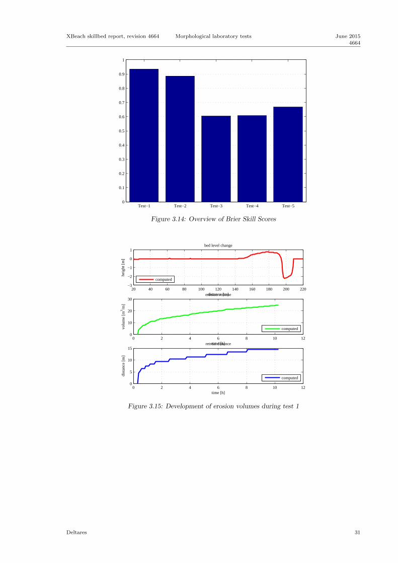
Five experiments are performed, as presented in Table 3.3. Tests 1, 2 and 5 had a constantsurge level, while tests 3 and 4 had a variable surge level with a course depicted in Figure 3.7
26 Deltares

XBeach skillbed report, revision 4664 Morphological laboratory tests June 2015
4664
and Figure 3.8 respectively.
Table 3.3: Overview of experiments
Experiment Scale Profile Sediment Water Wave Wavecontraction diameter depth height period
1 5 1.91 225 4.2 1.50 5.42 5 1.27 225 4.2 1.50 5.43 5 1.27 225 4.2 1.50 5.4
4 3.27 1.91 225 4.2 1.85 5.05 1 1 225 5.0 2.00 7.6
0 1 2 3 4 5 6 7 8
x 104
3
3.5
4
4.5
time [s]
wat
er le
vel [
m]
0 1 2 3 4 5 6 7 8
x 104
1
1.5
2
time [s]
wav
e he
ight
[m]
0 1 2 3 4 5 6 7 8
x 104
4.5
5
5.5
time [s]
peak
wav
e pe
riod
[s]
Figure 3.7: Boundary conditions for test 3
Deltares 27

June 2015
4664
Morphological laboratory tests XBeach skillbed report, revision 4664
0 1 2 3 4 5 6 7
x 104
3
3.5
4
4.5
time [s]
wat
er le
vel [
m]
0 1 2 3 4 5 6 7
x 104
1.4
1.6
1.8
2
time [s]
wav
e he
ight
[m]
0 1 2 3 4 5 6 7
x 104
4.5
5
5.5
6
time [s]
peak
wav
e pe
riod
[s]
Figure 3.8: Boundary conditions for test 4
As in the previous sections, the profile developments are compared to the measurements in?? to ??. Moreover, erosion patterns and volumes and retreat distances are analyzed inFigure 3.15 to Figure 3.19. Figure 3.14 provides an overview of the Brier Skill Scores of theprofile development for the different tests.
150 160 170 180 190 200 2102
2.5
3
3.5
4
4.5
5
5.5
6
6.5profiles Deltaflume_M1263_III Test−1
distance [m]
heig
ht [m
]
initialmeasuredXBeach (current) − BSS=0.94
Figure 3.9: Profile development during test 1
28 Deltares

XBeach skillbed report, revision 4664 Morphological laboratory tests June 2015
4664
160 165 170 175 180 185 190 195 200 205 2102
2.5
3
3.5
4
4.5
5
5.5
6
6.5profiles Deltaflume_M1263_III Test−2
distance [m]
heig
ht [m
]
initialmeasuredXBeach (current) − BSS=0.89
Figure 3.10: Profile development during test 2
150 160 170 180 190 200 2102
2.5
3
3.5
4
4.5
5
5.5
6
6.5profiles Deltaflume_M1263_III Test−3
distance [m]
heig
ht [m
]
initialmeasuredXBeach (current) − BSS=0.60
Figure 3.11: Profile development during test 3
Deltares 29

June 2015
4664
Morphological laboratory tests XBeach skillbed report, revision 4664
140 150 160 170 180 190 200 2101.5
2
2.5
3
3.5
4
4.5
5
5.5
6
6.5profiles Deltaflume_M1263_III Test−4
distance [m]
heig
ht [m
]
initialmeasuredXBeach (current) − BSS=0.61
Figure 3.12: Profile development during test 4
120 130 140 150 160 170 180 190 200 2101
2
3
4
5
6
7
8
9profiles Deltaflume_M1263_III Test−5
distance [m]
heig
ht [m
]
initialmeasuredXBeach (current) − BSS=0.67
Figure 3.13: Profile development during test 5
30 Deltares
XBeach skillbed report, revision 4664 Morphological laboratory tests June 2015
4664
Test−1 Test−2 Test−3 Test−4 Test−50
0.1
0.2
0.3
0.4
0.5
0.6
0.7
0.8
0.9
1
Figure 3.14: Overview of Brier Skill Scores
20 40 60 80 100 120 140 160 180 200 220−3
−2
−1
0
1bed level change
distance [m]
heig
ht [m
]
computed
0 2 4 6 8 10 120
10
20
30erosion volume
time [h]
volu
me
[m3 /m
]
computed
0 2 4 6 8 10 120
5
10
15retreat distance
time [h]
dist
ance
[m]
computed
Figure 3.15: Development of erosion volumes during test 1
Deltares 31

June 2015
4664
Morphological laboratory tests XBeach skillbed report, revision 4664
20 40 60 80 100 120 140 160 180 200 220−3
−2
−1
0
1bed level change
distance [m]
heig
ht [m
]
computed
0 2 4 6 8 10 120
5
10
15
20erosion volume
time [h]
volu
me
[m3 /m
]
computed
0 2 4 6 8 10 120
5
10
15retreat distance
time [h]
dist
ance
[m]
computed
Figure 3.16: Development of erosion volumes during test 2
0 50 100 150 200 250−3
−2
−1
0
1bed level change
distance [m]
heig
ht [m
]
computed
0 2 4 6 8 10 12 14 16 18 20−10
0
10
20erosion volume
time [h]
volu
me
[m3 /m
]
computed
0 2 4 6 8 10 12 14 16 18 200
5
10retreat distance
time [h]
dist
ance
[m]
computed
Figure 3.17: Development of erosion volumes during test 3
32 Deltares

XBeach skillbed report, revision 4664 Morphological laboratory tests June 2015
4664
−100 −50 0 50 100 150 200 250−3
−2
−1
0
1bed level change
distance [m]
heig
ht [m
]
computed
0 2 4 6 8 10 12 14 16 180
5
10
15erosion volume
time [h]
volu
me
[m3 /m
]
computed
0 2 4 6 8 10 12 14 16 180
5
10retreat distance
time [h]
dist
ance
[m]
computed
Figure 3.18: Development of erosion volumes during test 4
−100 −50 0 50 100 150 200 250−4
−2
0
2bed level change
distance [m]
heig
ht [m
]
computed
0 1 2 3 4 5 6 70
20
40
60
80erosion volume
time [h]
volu
me
[m3 /m
]
computed
0 1 2 3 4 5 6 70
10
20
30retreat distance
time [h]
dist
ance
[m]
computed
Figure 3.19: Development of erosion volumes during test 5
3.2 Large scale tests
This section discusses a selection of large scale laboratory experiments. The experimentsfocus on specific situations and processes that XBeach is assumed to model well.
Deltares 33

June 2015
4664
Morphological laboratory tests XBeach skillbed report, revision 4664
3.2.1 Revetments
Revetments or other hard structures influence the dune erosion process. Scour holes andwave runup on structures can occur, both important phenomena in the assessment of waterdefences. Scour holes are mainly caused due to the obstructed transport of sediments inseaward direction from the dune. A transport gradient causes a scour hole to occur. This isalso valid for other hard elements present in or near a dune. (Short) wave runup can causeovertopping of the revetment, which can cause erosion at the rear-side of the revetment.
3.2.1.1 Influence of reventment height
Steetzel (1987) describes a series of large scale experiments with revetments of differentheights. The experiments are performed in the Deltaflume of Delft Hydraulics, now knownas Deltares. A depthscale nd = 5 is used for all experiments (Vellinga, 1986) and the initialprofile in the flume correponds to the reference profile for the Holland coast. At the dunefoot, which was located at 193m from the wave board and 3.80m above the flumes floor, aconcrete revetment is applied that covers almost the whole dune face with a slope of 1:1.8.The lower end of the revetment is located at 2.5m above the flume floor. The location of thetop of the revetment varied in each experiment. The tests were conducted with a constantwater level of 4.2m and wave conditions that correspond to a Pierson-Moskowitz spectrumwith Hm0 = 1.50m and Tp = 4.20s. The sediment applied in the test had a median graindiameter of approximately D50 = 210µm. An overview of the tests is given in Table 3.4.
Table 3.4: Overview of experiments
Experiment Revetment height w.r.t. flume floor
T1 6.20mT2 5.40mT3 4.80m
The profile developments as measured and computed by XBeach are presented in Figure 3.20to Figure 3.22.
34 Deltares

XBeach skillbed report, revision 4664 Morphological laboratory tests June 2015
4664
Figure 3.20: Profile development during test T1
Figure 3.21: Profile development during test T2
Deltares 35

June 2015
4664
Morphological laboratory tests XBeach skillbed report, revision 4664
Figure 3.22: Profile development during test T3
3.2.2 Extreme conditions
This model test, described in Arcilla et al. (1994) (2E), concerns extreme conditions with araised water level at 4.6m above the flume bottom, a significant wave height, Hm0, of 1.4mand peak period, Tp, of 5s. Bed material consisted of sand with a D50 of approximately0.2mm. During the test substantial dune erosion took place.
Based on the integral wave parameters Hm0 and Tp and a standard Jonswap spectral shape,time series of wave energy were generated and imposed as boundary condition. Since theflume tests were carried out with first-order wave generation (no imposed super-harmonicsand sub-harmonics), the hindcast runs were carried out with the incoming bound long wavesset to zero as well. Active wave reflection compensation (ARC) was applied in the physicalmodel, which has a result similar to the weakly reflective boundary condition in XBeach,namely to prevent re-reflecting of outgoing waves at the wave paddle (offshore boundary).
A grid resolution of 1m was applied and the sediment transport settings were set at defaultvalues. For the morphodynamic testing the model was run for 0.8 hours of hydrodynamictime with a morphological factor of 10, effectively representing a morphological simulationtime of 8 hours.
In Figure 3.23 the hydrodynamic results are shown for first order wave generation (as in theflume tests).
36 Deltares

XBeach skillbed report, revision 4664 Morphological laboratory tests June 2015
4664
0 20 40 60 80 100 120 140 160 1800
0.5
1
1.5wave heights and water levels
heig
ht [
m]
distance [m]
wave height (HF,measured)wave height (LF,measured)wave height (measured)setup (measured)wave height (HF)wave height (LF)wave heightsetup
0 20 40 60 80 100 120 140 160 1800
0.2
0.4
0.6
0.8flow velocities
velo
city
[m
/s]
distance [m]
flow velocity (RMS,LF,measured)flow velocity (RMS,measured)flow velocity (RMS,LF)flow velocity (RMS)
Figure 3.23: Hydrodynamics during test 2E
In Figure 3.24 the horizontal distribution of sedimentation and erosion after 8 hours is shown,and the evolution in time of the erosion volume and the dune retreat. Noteworthy is theepisodic behaviour of the dune erosion, both in measurements and model. An importantconclusion for physical model tests is that for dune erosion it does make a difference whetherfirst-order or second-order wave steering is applied.
0 20 40 60 80 100 120 140 160 180 200−1.5
−1
−0.5
0
0.5bed level change
distance [m]
heig
ht [m
]
measuredcomputed
0 1 2 3 4 5 6 7 8−5
0
5
10erosion volume
time [h]
volu
me
[m3 /m
]
measuredcomputed
0 1 2 3 4 5 6 7 80
5
10retreat distance
time [h]
dist
ance
[m]
measuredcomputed
Figure 3.24: Morphodynamics during test 2E
A key element in the modelling is the avalanching algorithm; even though surfbeat wavesrunning up and down the upper beach are fully resolved by the model, without a mechanismto transport sand from the dry dune face to the beach the dune face erosion rate is substan-tially underestimated. The relatively simple avalanching algorithm implemented, whereby an
Deltares 37
June 2015
4664
Morphological laboratory tests XBeach skillbed report, revision 4664
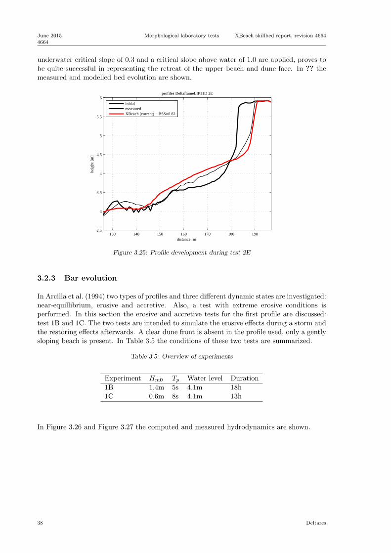
underwater critical slope of 0.3 and a critical slope above water of 1.0 are applied, proves tobe quite successful in representing the retreat of the upper beach and dune face. In ?? themeasured and modelled bed evolution are shown.
130 140 150 160 170 180 1902.5
3
3.5
4
4.5
5
5.5
6profiles DeltaflumeLIP11D 2E
distance [m]
heig
ht [m
]
initialmeasuredXBeach (current) − BSS=0.82
Figure 3.25: Profile development during test 2E
3.2.3 Bar evolution
In Arcilla et al. (1994) two types of profiles and three different dynamic states are investigated:near-equillibrium, erosive and accretive. Also, a test with extreme erosive conditions isperformed. In this section the erosive and accretive tests for the first profile are discussed:test 1B and 1C. The two tests are intended to simulate the erosive effects during a storm andthe restoring effects afterwards. A clear dune front is absent in the profile used, only a gentlysloping beach is present. In Table 3.5 the conditions of these two tests are summarized.
Table 3.5: Overview of experiments
Experiment Hm0 Tp Water level Duration
1B 1.4m 5s 4.1m 18h1C 0.6m 8s 4.1m 13h
In Figure 3.26 and Figure 3.27 the computed and measured hydrodynamics are shown.
38 Deltares

XBeach skillbed report, revision 4664 Morphological laboratory tests June 2015
4664
0 20 40 60 80 100 120 140 160 180 200−0.5
0
0.5
1wave heights and water levels
heig
ht [m
]
distance [m]
wave height (HF,measured)wave height (LF,measured)wave height (measured)setup (measured)wave height (HF)wave height (LF)wave heightsetup
0 20 40 60 80 100 120 140 160 180 2000
0.2
0.4
0.6
0.8flow velocities
velo
city
[m/s
]
distance [m]
flow velocity (RMS,LF,measured)flow velocity (RMS,measured)flow velocity (RMS,LF)flow velocity (RMS)
Figure 3.26: Hydrodynamics during test 1B
0 20 40 60 80 100 120 140 160 180−0.2
0
0.2
0.4
0.6wave heights and water levels
heig
ht [m
]
distance [m]
wave height (HF,measured)wave height (LF,measured)wave height (measured)setup (measured)wave height (HF)wave height (LF)wave heightsetup
0 20 40 60 80 100 120 140 160 1800
0.2
0.4
0.6
0.8flow velocities
velo
city
[m/s
]
distance [m]
flow velocity (RMS,LF,measured)flow velocity (RMS,measured)flow velocity (RMS,LF)flow velocity (RMS)
Figure 3.27: Hydrodynamics during test 1C
The profile development is shown in ?? and ??.
Deltares 39

June 2015
4664
Morphological laboratory tests XBeach skillbed report, revision 4664
140 150 160 170 180 190 200−1.5
−1
−0.5
0
0.5
1profiles DeltaflumeLIP11D 1B
distance [m]
heig
ht [m
]
initialmeasuredXBeach (current) − BSS=−0.90
Figure 3.28: Profile development during test 1B
130 140 150 160 170 180 190−1.5
−1
−0.5
0
0.5
1profiles DeltaflumeLIP11D 1C
distance [m]
heig
ht [m
]
initialmeasuredXBeach (current) − BSS=−1.27
Figure 3.29: Profile development during test 1C
3.2.4 Influence of wave period
In Van Gent et al. (2008) and Van Thiel de Vries et al. (2008) describe large-scale laboratoryexperiments on the influence of the wave period on the dune erosion process. It was concludedthat not only short waves, but also (wave group generated) long waves are important in thedune erosion process. Initially, about 30% of the dune erosion is due to long wave energy,but this amount increases with the development of an erosion profile. Moreover, an increaseof the wave period increases the dune erosion volumes.
XBeach, being a wave group solving model, is expected to be able to reproduce the observed
40 Deltares

XBeach skillbed report, revision 4664 Morphological laboratory tests June 2015
4664
influence of the wave period well. The following sections provide an in-depth comparisonof the first experiment from Van Gent et al. (2008). It continue with a comparison of theinfluence of the wave period and spectrum shape between the measurements obtained andthe XBeach results.
All experiments are performed in the Deltaflume of Delft Hydraulics, currently known asDeltares, using the reference profile for the Holland coast. This is a schematized profile thatis considered representative for the Holland coast. Furthermore, a significant wave height1.50m and a water depth of 4.50m is used. The test programme is given in Table 3.6. Duringtest T04 a profile with a double dune row is used.
Table 3.6: Overview of experiments
Experiment Tp Tm−1,0 Spectrum
T01 4.90 4.45 Pierson-MoskowitzT02 6.12 5.56 Pierson-MoskowitzT03 7.35 6.68 Pierson-MoskowitzT04 7.35 6.68 Pierson-Moskowitz
DP01 6.12 3.91 double-peakedDP02 7.35 5.61 double-peaked
3.2.4.1 Detailed analysis
In this section, a detailed comparison between simulated physics over an evolving bathymetryand the measurements obtained during the Deltaflume experiment in 2006 (Van Gent et al.,2008) is made. For brevity this comparison is performed only for test T01 (this test corre-sponds best to the Dutch normative conditions). The simulations are performed on a regulargrid with dx = 1m and input to the model are time series of short wave varying energy (lowpass filtered on the wave group time scale) and incoming (bound) long waves. The time seriesare constructed from pressure and flow measurements at x = 41m from the wave board. Theshort wave group velocity (associated with advection of wave action) is based on the Tm−1,0
wave period. Other model settings can be found in Van Thiel de Vries (2009).
Wave height transformation and wave setup (Figure 3.45) are favourably reproduced with themodel. The long wave height is slightly underestimated whereas the wave setup is slightlyoverestimated. The correlation between measured short wave variance and long wave watersurface elevations (Figure 3.31) corresponds reasonably well with the measurements. Towardsthe shoreline this correlation increases (Abdelrahman and Thornton, 1987; Roelvink andStive, 1989) meaning the highest short waves travel on top of long waves, which likely causesthat more short wave energy gets closer to the dune face.
Short wave skewness and asymmetry are reasonably predicted with the extended RieneckerFenton model (Figure 3.32, panel 1). However, in the inner surf zone both wave skewnessand asymmetry are overestimated. Possible explanations are wave breaking, which limits thesteepness and height of waves and the presence of free harmonics in the flume. Both theseeffects are not included in the wave shape model but indeed are present in the flume test(Van Thiel de Vries, 2009). From simulated skewness and asymmetry it follows that the totalnonlinearity of a short wave is overestimated close to the dune face (Figure 3.32, panel 2).The phase β is favourably simulated with the model but is underestimated further offshore.
Deltares 41

June 2015
4664
Morphological laboratory tests XBeach skillbed report, revision 4664
40 60 80 100 120 140 160 180 200 220−0.5
0
0.5
1
1.5wave heights and water levels
heig
ht [m
]
distance [m]
wave height (HF,measured)wave height (LF,measured)wave height (measured)setup (measured)wave height (HF)wave height (LF)wave heightsetup
40 60 80 100 120 140 160 180 200 220−0.5
0
0.5
1flow velocities
velo
city
[m/s
]
distance [m]
flow velocity (RMS,HF,measured)flow velocity (RMS,LF,measured)flow velocity (RMS,measured)flow velocity (u,mean,measured)flow velocity (RMS,HF)flow velocity (RMS,LF)flow velocity (RMS)flow velocity (u,mean)
Figure 3.30: Wave height transformations and flow velocities
40 60 80 100 120 140 160 180 200 220−0.8
−0.6
−0.4
−0.2
0
0.2
0.4
0.6
0.8correlations
corr
elat
ion ρ
[−]
distance [m]
correlation HF variance/LF elevation (measured)correlation HF variance/LF elevation
Figure 3.31: Correlation between short wave variance and long wave surface elevations
42 Deltares

XBeach skillbed report, revision 4664 Morphological laboratory tests June 2015
4664
40 60 80 100 120 140 160 180 200 220−2
−1.5
−1
−0.5
0
0.5
1wave shape
skew
ness
& a
sym
met
ry [−
]
distance [m]
wave skewness (measured)wave asymmetry (measured)wave skewnesswave asymmetry
40 60 80 100 120 140 160 180 200 220−2
−1
0
1
2wave nonlinearity
nonl
inea
rity
& p
hase
[−]
distance [m]
wave nonlinearity (measured)wave phase (measured)wave nonlinearitywave phase
Figure 3.32: Wave shape and nonlinearity
The simulated test and depth averaged flow velocity shows the same trend as in the mea-surements and increases towards the shoreline (Figure 3.33). However, in the simulation thecross-shore range with a high offshore mean flow is smaller and extends less far seaward thanin the measurements. This is possibly explained by differences in profile development (??)or inaccurate measurements. In addition, another explanation may be found in the incorrectmodeling of the roller energy dissipation. Simulations (not shown) with a smaller roller dis-sipation rate revealed that roller energy in the inner surf increases, leading to higher returnflow over a broader cross-shore range.
Long waves contribute to the time and depth averaged flow close to the shoreline. Thecontribution of long waves to the mean flow is explained by on average larger water depthsduring the interval associated with shoreward flow velocities in relation to the interval withoffshore flow velocities. Considering continuity and a uniform vertical structure of the longwave flow this means a time and depth averaged offshore directed flow should be present.
Nonlinear waves may cause onshore sediment transport presuming non-uniform sedimentstirring over the wave cycle and a positive correlation between sediment suspension and theintra wave flow. In order to include the wave averaged effect of nonlinear waves on thesediment transport a mean flow uA is computed, which is added to the mean (Eulerian) flowUm (Van Thiel de Vries, 2009). The simulated time averaged flow associated with nonlinearwaves shows a comparable evolution as in the measurements but is overestimated especiallycloser to the dune face. Near the shoreline the wave skewness related sediment transportvanishes (Figure 3.32, panel 1) since waves develop towards fully saw tooth shaped boresthat have negligible skewness.
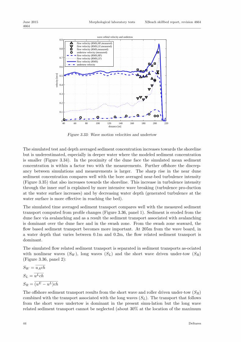
The orbital flow velocity (Figure 3.45, panel 2) is favourably predicted by the model. Theshort wave orbital flow velocity is slightly overestimated whereas the long wave orbital flowis underestimated. The underestimation of the simulated long wave orbital flow correspondswell to the slight underestimation of the observed long wave water surface variance.
Deltares 43
June 2015
4664
Morphological laboratory tests XBeach skillbed report, revision 4664
40 60 80 100 120 140 160 180 200 2200
0.1
0.2
0.3
0.4
0.5
0.6
0.7
0.8
0.9wave orbital velocity and undertow
velo
city
[m
/s]
distance [m]
flow velocity (RMS,HF,measured)flow velocity (RMS,LF,measured)flow velocity (RMS,measured)undertow velocity (measured)flow velocity (RMS,HF)flow velocity (RMS,LF)flow velocity (RMS)undertow velocity
Figure 3.33: Wave motion velocities and undertow
The simulated test and depth averaged sediment concentration increases towards the shorelinebut is underestimated, especially in deeper water where the modeled sediment concentrationis smaller (Figure 3.34). In the proximity of the dune face the simulated mean sedimentconcentration is within a factor two with the measurements. Further offshore the discrep-ancy between simulations and measurements is larger. The sharp rise in the near dunesediment concentration compares well with the bore averaged near-bed turbulence intensity(Figure 3.35) that also increases towards the shoreline. This increase in turbulence intensitythrough the inner surf is explained by more intensive wave breaking (turbulence pro-ductionat the water surface increases) and by decreasing water depth (generated turbulence at thewater surface is more effective in reaching the bed).
The simulated time averaged sediment transport compares well with the measured sedimenttransport computed from profile changes (Figure 3.36, panel 1). Sediment is eroded from thedune face via avalanching and as a result the sediment transport associated with avalanchingis dominant over the dune face and in the swash zone. From the swash zone seaward, theflow based sediment transport becomes more important. At 205m from the wave board, ina water depth that varies between 0.1m and 0.2m, the flow related sediment transport isdominant.
The simulated flow related sediment transport is separated in sediment transports as-ociatedwith nonlinear waves (SW ), long waves (SL) and the short wave driven under-tow (SR)(Figure 3.36, panel 2):
SW = uAch
SL = uLch
SR = (uE − uL)ch
The offshore sediment transport results from the short wave and roller driven under-tow (SR)combined with the transport associated with the long waves (SL). The transport that followsfrom the short wave undertow is dominant in the present simu-lation but the long waverelated sediment transport cannot be neglected (about 30% at the location of the maximum
44 Deltares

XBeach skillbed report, revision 4664 Morphological laboratory tests June 2015
4664
offshore transport). The wave related sediment transport (SW ) is onshore and suppresses theoffshore sediment transport with some 30%.
Profile evolution and dune erosion volumes are favourably predicted with the model duringtest T01 (?? and Figure 3.42, panel 2). Between t = 2.04 and 6.0 hours (interval E) the duneerosion rate is slightly underestimated. At the offshore edge of the developing foreshore,the model seems not capable to reproduce the steep transition from the original (unaffected)profile towards the newly developed foreshore. A bar type feature is observed at this transitionthat is hypothesized to be related to (partly) plunging breakers that generate a water jet,which penetrates in the water column and causes additional sediment stirring when it reachesthe bed. Though the effect of wave breaking induced turbulence on sediment suspension isincluded in the simulation, the applied model only considers spilling breakers, which areexpected to be less efficient than plunging breakers in stirring up sand.
40 60 80 100 120 140 160 180 200 2200
5
10
15
20
25
30sediment concentration
conc
entr
atio
n [g
/l]
distance [m]
concentration (measured)concentration
Figure 3.34: Sediment concentrations
Deltares 45

June 2015
4664
Morphological laboratory tests XBeach skillbed report, revision 4664
40 60 80 100 120 140 160 180 200 2200
0.2
0.4
0.6
0.8
1
1.2
1.4tubulence
tubu
lenc
e [m
2 /s2 ]
distance [m]
wave averaged tubulencebore averaged tubulencebore averaged near−bed turbulence
Figure 3.35: Wave induced turbulence
40 60 80 100 120 140 160 180 200 220−4
−2
0
2
4x 10
−4 sediment transport (morphodynamics)
tran
spor
t [m3 /m
/s]
distance [m]
bed level changes (measured)bed level changesavalanchingsuspendedbedload
40 60 80 100 120 140 160 180 200 220−3
−2
−1
0
1
2x 10
−4 sediment transport (hydrodynamics)
tran
spor
t [m3 /m
/s]
distance [m]
total hydrodynamicslong wavesshort wave undertowwave asymmetry
Figure 3.36: Sediment transports by transport type and forcing
46 Deltares

XBeach skillbed report, revision 4664 Morphological laboratory tests June 2015
4664
185 190 195 200 205 210 215−1.5
−1
−0.5
0
0.5
1
1.5
2profiles Deltaflume2006 T01
distance [m]
heig
ht [m
]
initialmeasuredXBeach (current) − BSS=0.94
Figure 3.37: Profile development
0 50 100 150 200 250−2
−1.5
−1
−0.5
0
0.5
1bed level change
distance [m]
heig
ht [m
]
measuredcomputed
0 1 2 3 4 5 6 70
2
4
6
8
10erosion volume
time [h]
volu
me
[m3 /m
]
measuredcomputed
Figure 3.38: Bed level changes and erosion volumes
It is concluded that profile evolution and dune erosion during test T01 are favourably simu-lated. Also simulated wave heights, flows, sediment concentrations and sediment transportscompare reasonably well with measurements. However,looking at the results in more detailsome discrepancies are found:
1. The long wave height and especially associated long wave orbital flows are un-derestimated.
2. The test and depth averaged flow between x = 170 m and x = 200 m is underestimated.Close to the shoreline no reliable measurements are available to verify the model results.
3. The simulated sediment concentration compares well with measurements close to the
Deltares 47

June 2015
4664
Morphological laboratory tests XBeach skillbed report, revision 4664
dune face. However, for smaller sediment concentrations in deeper water the simulatedconcentration is underestimated.
4. The offshore sediment transport is mainly driven by the short wave and roller inducedundertow (O(70%) at the location of the maximum offshore transport) whereas theoffshore directed long wave related sediment transport cancels out with the onshoresediment transport due to nonlinear short waves.
It is remarked that shoreward of the maximum offshore sediment transport, the importanceof the long wave related transport increases and eventually becomes dominant in relation tothe transport associated with short wave and roller driven undertow. Considering the mainlylong wave associated sediment transport in proximity of the dune face and the importanceof long wave run-up for avalanching it is expected that long waves are mainly responsible forthe swash zone sediment transport.
An overview of the Model Performance Statistics for test T01 with respect to the measure-ments is given in Table 3.7.
Table 3.7
R2 Sci Rel. bias BSS
zb 0.99 0.03 -0.01 0.94Hrmslf NaN NaN NaN NaNHrmshf NaN NaN NaN NaNrho 0.84 0.61 -0.44 0.70SK NaN NaN NaN NaNAS NaN NaN NaN NaNB NaN NaN NaN NaNbeta NaN NaN NaN NaNurmslf NaN NaN NaN NaNurmshf NaN NaN NaN NaNumean NaN NaN NaN NaNc NaN NaN NaN NaNdz 0.02 5002.69 73.47 -25989440.45
3.2.4.2 Wave period
During test T01, T02 and T03 of the 2006 Deltaflume experiment (Van Gent et al., 2008) theeffect of the wave period on dune erosion was examined. It was found that the dune erosionvolume increases for a larger wave period, which is caused by a larger flow related sedimenttransport. In addition, the increase in flow related sediment transport is mainly a result of ahigher mean sediment concentration whereas the time and depth averaged flow velocity hasthe same order of magnitude within the range of wave periods examined.
The aim of this section is to examine the processes, which cause the wave period effect inthe model and to what extent these processes are in line with the mechanisms observed inthe measurements. To this end test T01, T02 and T03 of the Deltaflume experiment aresimulated. The simulations are performed on a regular grid with dx = 1 m and input tothe model are time series of short wave varying energy (low pass filtered on the wave grouptime scale) and incoming (bound) long waves. The time series are constructed from pressureand flow measurements at x = 41 m from the wave board. The short wave group velocity
48 Deltares

XBeach skillbed report, revision 4664 Morphological laboratory tests June 2015
4664
(associated with advection of wave action) is based on the Tm−1,0 wave period. Settings forthe wave energy dissipation model are found in Table 3.8 and other setting are defaults aslisted in in Appendix B in Van Thiel de Vries (2009).
Table 3.8: Wave dissipation parameter settings
Experiment α γ n
T01 1.0 0.50 10T02 1.0 0.48 10T03 1.0 0.45 10
In ?? to ?? the simulated profile evolution during the tests compares well with the measuredprofile evolution. However, the bar type feature at the offshore edge of the developing fore-shore is not reproduced in the simulations. Comparing measured and simulated dune erosionvolumes in Figure 3.42 to Figure 3.44 it is seen that for test T03 the erosion volume after1 hour and 2.04 hours of waves is underestimated whereas for test T01 and T02 simulatederosion volumes are reasonably well predicted over all test intervals.
185 190 195 200 205 210 215−1.5
−1
−0.5
0
0.5
1
1.5
2profiles Deltaflume2006 T01
distance [m]
heig
ht [m
]
initialmeasuredXBeach (current) − BSS=0.94
Figure 3.39: Profile development during test T01
Deltares 49

June 2015
4664
Morphological laboratory tests XBeach skillbed report, revision 4664
180 185 190 195 200 205 210 215−1.5
−1
−0.5
0
0.5
1
1.5
2profiles Deltaflume2006 T02
distance [m]
heig
ht [m
]
initialmeasuredXBeach (current) − BSS=0.93
Figure 3.40: Profile development during test T02
180 185 190 195 200 205 210 215−1.5
−1
−0.5
0
0.5
1
1.5
2profiles Deltaflume2006 T03
distance [m]
heig
ht [m
]
initialmeasuredXBeach (current) − BSS=0.97
Figure 3.41: Profile development during test T03
50 Deltares

XBeach skillbed report, revision 4664 Morphological laboratory tests June 2015
4664
0 50 100 150 200 250−2
−1.5
−1
−0.5
0
0.5
1bed level change
distance [m]
heig
ht [m
]
measuredcomputed
0 1 2 3 4 5 6 70
2
4
6
8
10erosion volume
time [h]
volu
me
[m3 /m
]
measuredcomputed
Figure 3.42: Erosion pattern and volumes and retreat distance during test T01
0 50 100 150 200 250−2
−1.5
−1
−0.5
0
0.5
1bed level change
distance [m]
heig
ht [m
]
measuredcomputed
0 1 2 3 4 5 6 70
2
4
6
8
10
12erosion volume
time [h]
volu
me
[m3 /m
]
measuredcomputed
Figure 3.43: Erosion pattern and volumes and retreat distance during test T02
Deltares 51

June 2015
4664
Morphological laboratory tests XBeach skillbed report, revision 4664
0 50 100 150 200 250−2
−1.5
−1
−0.5
0
0.5
1bed level change
distance [m]
heig
ht [m
]
measuredcomputed
0 1 2 3 4 5 6 70
2
4
6
8
10
12erosion volume
time [h]
volu
me
[m3 /m
]
measuredcomputed
Figure 3.44: Erosion pattern and volumes and retreat distance during test T03
Simulated time and depth averaged flows are compared in Figure 3.45 to Figure 3.47, whichshows that the mean flow slightly increases with a larger wave period (6% between x = 170 mand x = 205 m). This tends to be a slightly different trend than observed in the measurementsthat show a 3% increase in the same cross-shore area. It is remarked though that any firmconclusions cannot be made since the measured time and depth averaged flow velocities arebased on limited sensors over depth (and for that reason it was concluded that the meanflows for test T01 and T03 are comparable).
The increase in the simulated offshore directed mean flow is caused by an increase of theshort wave related mass flux whereas the roller related mass flux is only slightly different.The maximum long wave related mean flow is larger during test T01 than during test T03.
40 60 80 100 120 140 160 180 200 220−0.5
0
0.5
1
1.5wave heights and water levels
heig
ht [m
]
distance [m]
wave height (HF,measured)wave height (LF,measured)wave height (measured)setup (measured)wave height (HF)wave height (LF)wave heightsetup
40 60 80 100 120 140 160 180 200 220−0.5
0
0.5
1flow velocities
velo
city
[m/s
]
distance [m]
flow velocity (RMS,HF,measured)flow velocity (RMS,LF,measured)flow velocity (RMS,measured)flow velocity (u,mean,measured)flow velocity (RMS,HF)flow velocity (RMS,LF)flow velocity (RMS)flow velocity (u,mean)
Figure 3.45: Hydrodynamics during test T01
52 Deltares

XBeach skillbed report, revision 4664 Morphological laboratory tests June 2015
4664
40 60 80 100 120 140 160 180 200 220−0.5
0
0.5
1
1.5wave heights and water levels
heig
ht [m
]
distance [m]
wave height (HF,measured)wave height (LF,measured)wave height (measured)setup (measured)wave height (HF)wave height (LF)wave heightsetup
40 60 80 100 120 140 160 180 200 220−0.5
0
0.5
1flow velocities
velo
city
[m/s
]
distance [m]
flow velocity (RMS,HF,measured)flow velocity (RMS,LF,measured)flow velocity (RMS,measured)flow velocity (u,mean,measured)flow velocity (RMS,HF)flow velocity (RMS,LF)flow velocity (RMS)flow velocity (u,mean)
Figure 3.46: Hydrodynamics during test T02
40 60 80 100 120 140 160 180 200 220−0.5
0
0.5
1
1.5wave heights and water levels
heig
ht [m
]
distance [m]
wave height (HF,measured)wave height (LF,measured)wave height (measured)setup (measured)wave height (HF)wave height (LF)wave heightsetup
40 60 80 100 120 140 160 180 200 220−0.5
0
0.5
1flow velocities
velo
city
[m/s
]
distance [m]
flow velocity (RMS,HF,measured)flow velocity (RMS,LF,measured)flow velocity (RMS,measured)flow velocity (u,mean,measured)flow velocity (RMS,HF)flow velocity (RMS,LF)flow velocity (RMS)flow velocity (u,mean)
Figure 3.47: Hydrodynamics during test T03
It is concluded that the effect of the wave period on dune erosion and dune face retreat isfavourably predicted with the XBeach model. The simulated increase in dune erosion witha larger wave period is mainly caused by an increase of the mean sediment concentrationof O(60%), which is comparable to the measurements. The near dune return flow slightlyincreases with approximately 6% for a larger wave period. However, the accuracy of measuredtime and depth averaged flows is insufficient to verify this increase.
Deltares 53
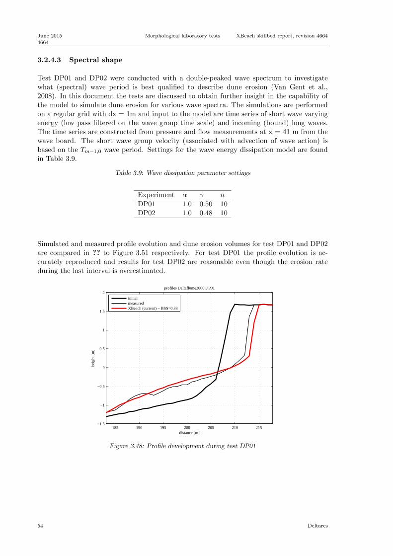
June 2015
4664
Morphological laboratory tests XBeach skillbed report, revision 4664
3.2.4.3 Spectral shape
Test DP01 and DP02 were conducted with a double-peaked wave spectrum to investigatewhat (spectral) wave period is best qualified to describe dune erosion (Van Gent et al.,2008). In this document the tests are discussed to obtain further insight in the capability ofthe model to simulate dune erosion for various wave spectra. The simulations are performedon a regular grid with dx = 1m and input to the model are time series of short wave varyingenergy (low pass filtered on the wave group time scale) and incoming (bound) long waves.The time series are constructed from pressure and flow measurements at x = 41 m from thewave board. The short wave group velocity (associated with advection of wave action) isbased on the Tm−1,0 wave period. Settings for the wave energy dissipation model are foundin Table 3.9.
Table 3.9: Wave dissipation parameter settings
Experiment α γ n
DP01 1.0 0.50 10DP02 1.0 0.48 10
Simulated and measured profile evolution and dune erosion volumes for test DP01 and DP02are compared in ?? to Figure 3.51 respectively. For test DP01 the profile evolution is ac-curately reproduced and results for test DP02 are reasonable even though the erosion rateduring the last interval is overestimated.
185 190 195 200 205 210 215−1.5
−1
−0.5
0
0.5
1
1.5
2profiles Deltaflume2006 DP01
distance [m]
heig
ht [m
]
initialmeasuredXBeach (current) − BSS=0.88
Figure 3.48: Profile development during test DP01
54 Deltares
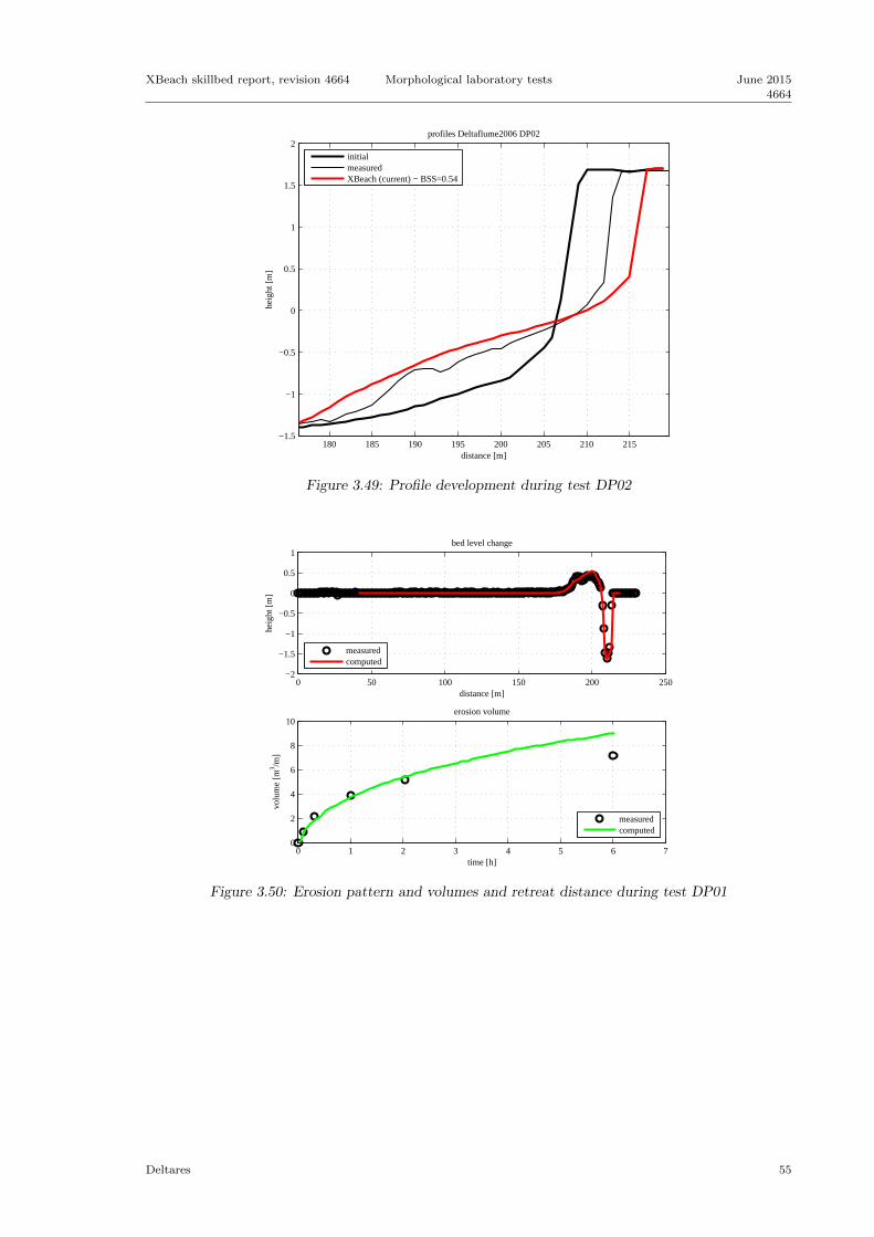
XBeach skillbed report, revision 4664 Morphological laboratory tests June 2015
4664
180 185 190 195 200 205 210 215−1.5
−1
−0.5
0
0.5
1
1.5
2profiles Deltaflume2006 DP02
distance [m]
heig
ht [m
]
initialmeasuredXBeach (current) − BSS=0.54
Figure 3.49: Profile development during test DP02
0 50 100 150 200 250−2
−1.5
−1
−0.5
0
0.5
1bed level change
distance [m]
heig
ht [m
]
measuredcomputed
0 1 2 3 4 5 6 70
2
4
6
8
10erosion volume
time [h]
volu
me
[m3 /m
]
measuredcomputed
Figure 3.50: Erosion pattern and volumes and retreat distance during test DP01
Deltares 55

June 2015
4664
Morphological laboratory tests XBeach skillbed report, revision 4664
0 50 100 150 200 250−2
−1.5
−1
−0.5
0
0.5
1bed level change
distance [m]
heig
ht [m
]
measuredcomputed
0 1 2 3 4 5 6 70
5
10
15erosion volume
time [h]
volu
me
[m3 /m
]
measuredcomputed
Figure 3.51: Erosion pattern and volumes and retreat distance during test DP02
The imposed double-peaked wave spectra affect the time scale and amplitude of the simulatedwave groups. Consequently, the interaction of simulated long waves with the short wavegroups is different and hydrodynamics in front of the dune face are expected to have othercharacteristics. In Figure 3.52 and Figure 3.53 the simulated wave transformation, flows andsediment concentrations are favourably compared with measurements obtained during testDP01. It seems the model is capable to take into account the effect of various wave spectraon near dune hydrodynamics and sediment transports.
40 60 80 100 120 140 160 180 200 220−0.5
0
0.5
1wave heights and water levels
heig
ht [m
]
distance [m]
wave height (HF,measured)wave height (LF,measured)wave height (measured)setup (measured)wave height (HF)wave height (LF)wave heightsetup
40 60 80 100 120 140 160 180 200 220−0.5
0
0.5
1flow velocities
velo
city
[m/s
]
distance [m]
flow velocity (RMS,HF,measured)flow velocity (RMS,LF,measured)flow velocity (RMS,measured)flow velocity (u,mean,measured)flow velocity (RMS,HF)flow velocity (RMS,LF)flow velocity (RMS)flow velocity (u,mean)
Figure 3.52: Hydrodynamics during test DP01
56 Deltares

XBeach skillbed report, revision 4664 Morphological laboratory tests June 2015
4664
40 60 80 100 120 140 160 180 200 220−0.5
0
0.5
1wave heights and water levels
heig
ht [m
]
distance [m]
wave height (HF,measured)wave height (LF,measured)wave height (measured)setup (measured)wave height (HF)wave height (LF)wave heightsetup
40 60 80 100 120 140 160 180 200 220−0.5
0
0.5
1flow velocities
velo
city
[m/s
]
distance [m]
flow velocity (RMS,HF,measured)flow velocity (RMS,LF,measured)flow velocity (RMS,measured)flow velocity (u,mean,measured)flow velocity (RMS,HF)flow velocity (RMS,LF)flow velocity (RMS)flow velocity (u,mean)
Figure 3.53: Hydrodynamics during test DP02
It is concluded that the effect of the wave spectral shape on dune erosion and dune face retreatis favourably predicted with the model. The time averaged simulated wave transformation,flow and sediment concentration compare well with the mobile frame measurements obtainedduring test DP01.
In Van Gent et al. (2008) the spectral mean wave period Tm−1,0 is argued to be more qualifiedto describe dune erosion than the peak wave period Tp. The simulations presented in thissubsection are performed with the Tm−1,0 wave period and show satisfying results suggestingthe spectral mean wave period proposed by Van Gent et al. (2008) is indeed a good measureto describe dune erosion. It is remarked though that any firm conclusion would require extrasimulations in which the peak wave period Tp is applied instead of the Tm−1,0 wave period. Inaddition this would demand for a new model optimization and most likely different settingsfor the wave dissipation model.
3.2.4.4 Double dune system
Test T04 of the Deltaflume experiment 2006 (Van Gent et al., 2008) is carried out with aninitial profile that contains a small dune in front of a larger volume dune that collapses afterapproximately one hour of waves (interval C and D). After breaching of the small dune,the foreshore is already very efficient in reducing wave impacts on the dune face resulting insmall erosion rates over the remaining test intervals. In this test it is examined to what extentthe dune breach can be reproduced with the XBeach model and whether the (substantiallysmaller) erosion rate at the end of a storm is correctly predicted. The simulations is performedon a regular grid with dx = 1 m and input to the model are time series of short wave varyingenergy (low pass filtered on the wave group time scale) and incoming (bound) long waves.The time series are constructed from pressure and flow measurements at x = 41 m from thewave board. The short wave group velocity (associated with advection of wave action) isbased on the Tm−1,0 wave period. Settings for the wave energy dissipation model are equalto the settings for the T03 test.
Simulated profile evolution and dune erosion volumes are shown in ?? and Figure 3.55 re-
Deltares 57

June 2015
4664
Morphological laboratory tests XBeach skillbed report, revision 4664
spectively. The simulated hydrodynamics are presented in Figure 3.56. For the first threeintervals (the small dune breaches in interval 3) the dune erosion rate is slightly overestimatedbut the profile evolution compares favourably with the measured profiles. Considering thelast two intervals, erosion rates and dune face retreat are too large.
Breaching of a small dune in front of a larger volume dune causes that suddenly the foreshoreis significantly closer to equilibrium with the storm surge conditions. As a result near shorehydrodynamics, near shore sediment transports and wave impacts on the dune face are lesssevere. It is concluded that the feedback between profile evolution and near dune processesis not sufficiently well included in the model at the end of test T04, which is representativefor conditions at the end of a storm. More insight in the model performance at the end of astorm could possibly be obtained by comparing the evolution of simulated driving processes(undertow, sediment concentrations and avalanching) with measurements.
60 80 100 120 140 160 180 200 220−4
−3
−2
−1
0
1
2profiles Deltaflume2006 T04
distance [m]
heig
ht [m
]
initialmeasuredXBeach (current) − BSS=0.87
Figure 3.54: Profile development during test T04
58 Deltares

XBeach skillbed report, revision 4664 Morphological laboratory tests June 2015
4664
0 50 100 150 200 250−2
−1.5
−1
−0.5
0
0.5bed level change
distance [m]
heig
ht [m
]
measuredcomputed
0 1 2 3 4 5 6 70
2
4
6
8erosion volume
time [h]
volu
me
[m3 /m
]
measuredcomputed
Figure 3.55: Erosion pattern and volumes and retreat distance during test T04
40 60 80 100 120 140 160 180 200 220−0.5
0
0.5
1
1.5wave heights and water levels
heig
ht [m
]
distance [m]
wave height (HF,measured)wave height (LF,measured)wave height (measured)setup (measured)wave height (HF)wave height (LF)wave heightsetup
40 60 80 100 120 140 160 180 200 220−0.5
0
0.5
1flow velocities
velo
city
[m/s
]
distance [m]
flow velocity (RMS,HF,measured)flow velocity (RMS,LF,measured)flow velocity (RMS,measured)flow velocity (u,mean,measured)flow velocity (RMS,HF)flow velocity (RMS,LF)flow velocity (RMS)flow velocity (u,mean)
Figure 3.56: Hydrodynamics during test T04
Deltares 59

June 2015
4664
Morphological laboratory tests XBeach skillbed report, revision 4664
60 Deltares
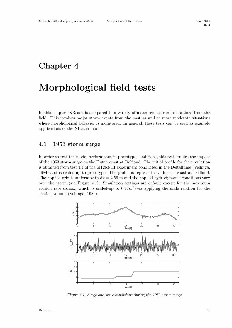
XBeach skillbed report, revision 4664 Morphological field tests June 2015
4664
Chapter 4
Morphological field tests
In this chapter, XBeach is compared to a variety of measurement results obtained from thefield. This involves major storm events from the past as well as more moderate situationswhere morphological behavior is monitored. In general, these tests can be seen as exampleapplications of the XBeach model.
4.1 1953 storm surge
In order to test the model performance in prototype conditions, this test studies the impactof the 1953 storm surge on the Dutch coast at Delfland. The initial profile for the simulationis obtained from test T4 of the M1263-III experiment conducted in the Deltaflume (Vellinga,1984) and is scaled-up to prototype. The profile is representative for the coast at Delfland.The applied grid is uniform with dx = 4.56 m and the applied hydrodynamic conditions varyover the storm (see Figure 4.1). Simulation settings are default except for the maximumerosion rate dzmax, which is scaled-up to 0.17m3/ms applying the scale relation for theerosion volume (Vellinga, 1986).
0 5 10 15 20 25 300
1
2
3
4
5
time [h]
η [m
]
0 5 10 15 20 25 300
5
10
time [h]
Hrm
s [m]
0 5 10 15 20 25 308
9
10
11
12
time [h]
Tp [s
]
Figure 4.1: Surge and wave conditions during the 1953 storm surge
Deltares 61

June 2015
4664
Morphological field tests XBeach skillbed report, revision 4664
The simulated profile evolution is shown in ??. Evolution of the simulated dune erosionvolume is shown in Figure 4.3.
1100 1150 1200 1250 1300 135015
20
25
30profiles 1953_storm_surge default
distance [m]
heig
ht [m
]
initialXBeach (current)
Figure 4.2: Profile development
0 500 1000 1500−6
−4
−2
0
2bed level change
distance [m]
heig
ht [m
]
computed
0 5 10 15 20 25 30 350
50
100
150erosion volume
time [h]
volu
me
[m3 /m
]
computed
0 5 10 15 20 25 30 350
5
10
15
20retreat distance
time [h]
dist
ance
[m]
computed
Figure 4.3: Morphological response
4.2 1976 storm surge
This test studies the impact of the 1976 storm surge on the Dutch coast at Holland. Thesurge during the 1976 storm was the highest since the 1953 storm. In the night betweenJanuary 2nd and 3rd wind speeds reached a maximum near the Dutch coast. In the centraland eastern parts of the North Sea the wind speed reached 51 m/s from the Northwest. The
62 Deltares

XBeach skillbed report, revision 4664 Morphological field tests June 2015
4664
strongest gale on the Dutch mainland was recorded at Vlissingen: southwestern wind with aspeed of 26 m/s. This caused a significant storm surge with a maximum water level in theafternoon of January 3rd (Van der Werf et al., 2011).
Between October 1975 (pre-storm) and February (post-storm) 1976 30 cross-shore profilemeasurements were performed at eight locations (among others) along the North-Hollandcoast. The observed profiles generally extend from the low water line to above the dunefoot (+3 m NAP). We have extended these with the latest JARKUS data (yearly profilemeasurement from approximately -8 m NAP to the first dune row), measured in spring 1975.1D XBeach models were setup for these 30 transects, of which 3 are used in this test.
We base the XBeach model settings on an extensive sensitivity analysis and on recent XBeachstudies (Van der Werf and Van Santen, 2010). Furthermore, we take a morphological accel-eration factor of 1, set the offshore boundary at a depth of 20 m, and use measured insteadof computed water levels as input.
As an example, Figure 4.4 shows the initial cross-shore profile with the pre-storm measure-ment, the post-storm measurement and the final profile predicted by XBeach for one of the30 transects. ?? shows the Brier Skill Score of all computed transects.
−400 −300 −200 −100 0 100−10
−5
0
5
10
15
20profiles 1976_storm_surge raai3400
distance [m]
heig
ht [m
]
initialmeasuredXBeach (current) − BSS=0.54
Figure 4.4: raai3400
Deltares 63

June 2015
4664
Morphological field tests XBeach skillbed report, revision 4664
raai3400 raai568 raai60500
0.1
0.2
0.3
0.4
0.5
0.6
0.7
0.8
0.9
1
Figure 4.5: Overview of Brier Skill Scores
4.3 Erosion and overwash of Asseteague Island
This test concerns the morphodynamic response of sandy dunes to extreme storm impactsat Assateague Island, Maryland, USA, which was analyzed before by Jimenez et al. (2006).Two consecutive North Easters attacked the barrier island during late January and earlyFebruary, 1998. The bathymetry was measured using LIDAR in September 1997 and againFebruary 9th and 10th, 1998 after the two storms had subsided.
Three types of dunes were identified by Jimenez et al. (2006), shown in Figure 4.6. Profile A(upper left panel) is initially characterized by a steep faced dune, where the maximum run-upexceeded the dune crest height and the mildly sloped back of the dune. The morphologicalresponse is characterised by profile lowering, decrease of the beach face slope and landwardbarrier displacement, while retaining barrier width.
Profile type B is a double-peaked dune profile and has two different shapes. Profile B1 (upperright panel) is initially characterized by a primary and secondary dune, both of which arelower than the maximum run-up height and which are separated by a valley. Profile B2(bottom left panel) initially has two peaks of which the seaward one is lower. The backsideof the barrier of either type is therefore either characterized by a secondary dune line (profileB1) or a taller crest of the dune (profile B2) which prevents the eroded sand from beingtransported to the backside of the dune. The main morphological response for these profiletypes is a decrease of the beach face slope, outer shoreline retreat and narrowing of thebarrier.
The height of the dune crest of profile C (lower right panel) exceeds the maximum run-upheight and so little overwash is observed. The morphological response of this type of profileis crest lowering due to slumping, decrease of the beach face slope and retreat of the outershoreline. The width of the barrier is seen to decrease.
The storm impact of the two North Easters on Assateague Island were modelled with XBeachfor the four profiles described by Jimenez et al. (2006). The profiles were extended with
64 Deltares

XBeach skillbed report, revision 4664 Morphological field tests June 2015
4664
a shallow foreshore and a 1:100 slope in seaward direction till a water depth of 9 m belowNAVD88. As XBeach has not been shown to accurately simulate morphological change duringvery long storm durations, the simulations were run for a total of 20 hours. The measuredwave and surge conditions were parameterized for each storm by a constant surge level anda constant wave spectrum (Pierson-Moskowitz) (see Table 4.1). This approach assumes thattwo 72 hour storms with varying surge and wave conditions can be approximated by two10 hour simulations with constant maximum surge and wave conditions following a similarapproach as Vellinga (1986). This approach also facilitates further sensitivity studies intothe effect of varying hydraulic forcing conditions. The calculation grid size varies from 18 mat the offshore boundary to 2 m on the islands. A morphological acceleration factor of 5 isapplied. The final simulated bed profiles are shown in Figure 4.6.
Table 4.1: Hydrodynamic boundary conditions XBeach simulations
Storm 1 Storm 2
Surge level [m +NAVD] 0.8 1.0Hs [m] 4.1 3.9Tp [s] 8.5 8.5
800 1000 1200 1400−3
−2
−1
0
1
2
3
ProfileA
x (m)
Ele
vatio
n (m
+N
AV
D88
)
800 1000 1200 1400−3
−2
−1
0
1
2
3
ProfileB1
x (m)
Ele
vatio
n (m
+N
AV
D88
)
800 1000 1200 1400−3
−2
−1
0
1
2
3
ProfileB2
x (m)
Ele
vatio
n (m
+N
AV
D88
)
800 1000 1200 1400−3
−2
−1
0
1
2
3
ProfileC
x (m)
Ele
vatio
n (m
+N
AV
D88
)
Figure 4.6: Pre-storm profiles (black dotted line), measured post-storm profiles (blacksolid line) and modelled post-storm profiles (red solid line). Upper left panel: profile A.Upper right panel: profile B1. Lower left panel: profile B2. Lower right panel: profile C.The seaward side is on the left in all panels. Note that the measured post-storm profilescontain only the sea surface and emerged topography and no submerged topography.
4.4 Breach growth at Zwin
This test is absed on the Zwin breach growth experiment, as reported by Visser (1998). Inthe mouth of the Zwin, a tidal inlet located at the border between the Netherlands andBelgium, an artificial dam was constructed with a crest height of 3.3 m +N.A.P. (Dutchdatum, approx. MSL), crest width 8 m, inner slope 1:3 outer slope 1:1.6 and length 250 m.
Deltares 65

June 2015
4664
Morphological field tests XBeach skillbed report, revision 4664
An initial depression of 0.8 m was made in the middle of the dam having a width of 1 mand a side slope of 1:1.6 to ensure that the breach initiated at this location. The level of thesurrounding sea bed was about 0.7 m + N.A.P. The mean tidal prism of the Zwin is about350,000 m3. The polder area Ap as a function of the water level behind the dam is given by:
Ap = 170.000m · zs − 100.000m2 , 0.6m < zs < 2.3m+NAPAp = 2.100.000m · zs − 4.540.000m2 , zs ≥ 2.3m+NAP
At t = 0, about 10 minutes prior to high water, the water level at the seaside was 2.72m+NAP.At t = 10 minutes a water level of 2.75m+NAP. was reached. For the remainder of the test,which had a total duration of 1 hour, the water level marginally decreased. After 1 hour thebreach growth became nil, as the water level of the polder area behind the breached equaledthe sea level. The wave height near the dam was negligible during the experiment. The windspeed was about 2 m/s.
Until t = 6.5 minutes the breach depth grew whereas the breach width remained constant.At t = 6.5 minutes the original dike structure had nearly completely disappeared over theinitial depression width of 1 m. Near t = 6.5 minutes the onset of lateral breach growth wasobserved. The scour hole developed further down to a depth of -1.6m+NAP. (4.9 m belowthe original dam crest level). The rate of lateral breach growth was about 2 cm/s. Afterapproximately 40 minutes the process slowed down considerably and after approximately 1hour the water levels at both sides were equal.
A schematized representation of the Zwin test was created in XBeach, with at the sea sidea uniform bed level at 0.7m+NAP, and inside the basin a prismatic profile with the deepestpoint at 0.7m+NAP and sloping sides, such that the polder area as a function of the waterlevel was in accordance with the equations above. The grid is non-equidistant with grid sizesgradually varying from 0.5 m near the breach to approx. 50 m far away from it. The mediangrain diameter D50 of the bed material was set to 0.3 mm in accordance with the prototypetest conditions for the artificial dam. The applied critical slopes for avalanching are the sameas in other tests and standard settings were applied for the transport formulations. Waveswere negligible in the test and were set to zero. The model was run with a CFL of 0.5 andremained smooth and stable despite the steep slopes and supercritical flows.
In Figure 4.7 a sequence of 3D images is shown depicting the various stages in the breachingprocess: the initial overflowing, the cutting back of the breach, the deepening and finally thewidening of the breach.
66 Deltares
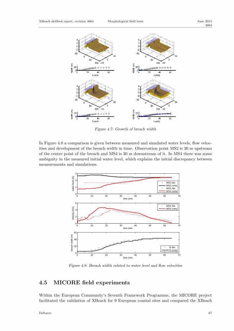
XBeach skillbed report, revision 4664 Morphological field tests June 2015
4664
Figure 4.7: Growth of breach width
In Figure 4.8 a comparison is given between measured and simulated water levels, flow veloc-ities and development of the breach width in time. Observation point MS2 is 30 m upstreamof the centre point of the breach and MS4 is 30 m downstream of it. In MS4 there was someambiguity in the measured initial water level, which explains the initial discrepancy betweenmeasurements and simulations.
0 10 20 30 40 50 60 700
1
2
3
time (min.
wat
er le
vel (
m)
MS2 obsMS2 compMS4 obsMS4 comp
0 10 20 30 40 50 60 700
2
4
6
time (min.
velo
city
(m
/s)
MS4 obsMS4 comp
0 10 20 30 40 50 60 700
20
40
60
time (min.
brea
ch w
idth
(m
)
B obsB comp
Figure 4.8: Breach width related to water level and flow velocities
4.5 MICORE field experiments
Within the European Community’s Seventh Framework Programme, the MICORE projectfacilitated the validation of XBeach for 9 European coastal sites and compared the XBeach
Deltares 67

June 2015
4664
Morphological field tests XBeach skillbed report, revision 4664
results to results obtained from models locally used (Deltares, 2011).
The validation of XBeach started off with a measurement campaign at each of the 9 sites.During the measurements, bathymetric and hydrodynamic data is collected, which is subse-quently used as input for XBeach and the other models. The following subsections describethe results for 6 of the 9 field sites.
4.5.1 Lido di Dante, Italy
The study site is the Lido di Dante-Lido di Classe area, an 8 km stretch of sandy beaches alongthe Emilia-Romagna coastline in northern Italy on the Adriatic Sea. The site is a mixture ofurbanised (approximately 40% of the total area) and relatively pristine (approximately 60%)coastal environments. The seaside towns of Lido di Dante and Lido di Classe are located atthe site’s northern and southern boundaries respectively. In these regions the beaches areprotected by offshore breakwaters and groins and backed by moderate coastal development inthe form of beach huts, holiday accommodation and paved roads. Between these two townsis a natural park consisting of natural vegetated dunes and no coastal protection. Three rivermouths are located at the site: one at Lido di Dante (Fiumi Uniti); one at Lido di Classe(Fiume Savio); and one in the centre of the natural park (Torrente Bevano).
The submerged beach is generally composed of fine sand, while the beachface is made up offine to medium sands (D50 = 0.03 mm). The intertidal beach slope varies significantly alongthe 8 km’s of coastline, from mild (2.5%) to steep (14%). Steep values are representative ofareas adjacent to coastal defence structures (i.e. groins) while the area inside the natural parkis characterised by lower gradients. The mean submerged beach slope is 3%. According tothe morphodynamic classification of Wright and Short (1984), the beaches are considered ashaving intermediate beach states. Low tide terraces are often observed both in the protectedand natural areas. Submerged longshore bars meanwhile are only present in the areas outsideof the offshore structures.
The wave climate of this region is generally small, with 91% of significant wave heights below1.25 m. The prevalent wave direction is from the east, while the most intense storms are fromthe ENE (known as the ”Bora wind”). The Bora wind is a strong, cold, gusty wind that blowsintermittently but mainly during the winter months. It not only has a strong influence onthe wave climate of this region, but of the general circulation patterns of the entire AdriaticSea. South-easterly waves meanwhile are much less significant, since SE winds are shelteredto some degree by the Conero Headland approximately 120 km south of the site.
In regards to water level variations, the area is microtidal with a mean neap tidal rangeof 30-40 cm and a mean spring tidal range of 80-90 cm. The tidal signal has both diurnaland semidiurnal components. Tidal anomalies of up to double the maximum tidal elevationcan occur as a result of surge. This is particularly the case during SE wind conditions,where, considering the SE-NE orientation of the Adriatic Sea, there is the greatest fetch forwind-driven surge.
Within the 2008-2010 MICORE monitoring period, three storms were selected for calibrationof the off-the-shelf and XBeach models. Each storm has distinct properties that encompassthe range of storm conditions typical for the Emilia-Romagna region. Here the modelling isrestricted to profile MN15 for the 1-3 December 2008 storm.
68 Deltares

XBeach skillbed report, revision 4664 Morphological field tests June 2015
4664
−4650−4600−4550−4500−4450−4400−4350−4300−4
−3
−2
−1
0
1
2
3
4profiles
distance [m]
heig
ht [m
]
initialmeasuredXBeach − BSS=0.16XBeach (current) − BSS=−4.06
Figure 4.9
4.5.2 Praia de Faro, Portugal
The study area is Ancao Peninsula constituting the westernmost barrier of the Ria Formosabarrier island system. It is a NW-SE oriented sandy barrier that is attached to mainland byits western terminus.
The area is mesotidal, with an average tidal range of about 2 m that can reach up to 3.5 mduring spring tides. Analysis of two years of records from a tidal gauge on the Algarve Coastshowed a maximum observed storm surge level of +0.75 m (Gama et al., 1994). The returnperiod of a sea level 2.23 m above Mean Sea Level (MSL) is 10 years (Gama et al., 1994).
The offshore wave climate is dominated by west-southwest waves (71% of occurrences). SEwaves that consist of short period waves generated by regional winds (locally called ’Levante’)are also frequent (about 23%). Wave energy is moderate with an average annual significantoffshore wave height of 1.0 m and average peak period of 8.2 s (Costa et al., 2001).
Storm events in the region are considered when the significant offshore wave height exceeds 3m (Pessanha and Pires, 1981) and typically correspond to less than 1% of the offshore waveclimate (Costa et al., 2001). A 5.0 m significant wave height for a SE storm has a returnperiod of 50 years, whilst a 5.7 m SW storm is expected every 5 years (Pires, 1998). Due toit’s northwest-southeast orientation it is directly exposed to west-southwesterly waves, andis relatively protected from SE waves.
Several storm events have been recorded during the MICORE campaign among which thetwo most important are discussed in the MICORE report. Here a group of several individualWSW storms is simulated that took place at Faro beach from 18/12/2009 until 5/1/2010.The significant wave height reached 4 m and the peak period up to 20 sec, while given thelong duration intense wave conditions coincided with both spring and neap tides. The eventhad a significant impact on the coast, as overtopping and dune erosion occurred at severalsections.
Deltares 69

June 2015
4664
Morphological field tests XBeach skillbed report, revision 4664
1200 1250 1300 1350 1400 1450 1500 1550 1600−4
−2
0
2
4
6
8
10profiles
distance [m]
heig
ht [m
]
initialmeasuredother − BSS=0.30XBeach − BSS=0.44XBeach (current) − BSS=−0.89
Figure 4.10
4.5.3 Cadiz Urban Beach, Spain
The field site is located around Cadiz town, in south-western Spain, facing the Atlantic Ocean.It is constituted by two different beaches extending along 10 km, providing the opportunityfor studying the effects of storms on different types of coastal environments.
The study area is a mesotidal coast with a mean tidal range of 3.2 m and 1.1 m duringsprings and neaps tides, respectively. Dominant winds blow from ESE (19.6% of annualoccurrence) and WNW (12.8%), which together with coastline orientation makes sea and swellwaves approach generally from the third and fourth quadrants. According to this, prevailinglongshore drift is directed south-eastwards. Significant wave height is usually lower than 1m, with waves over 4 m high being uncommon and occurring only during the most importantstorms, which usually take place between November and March and approach from the thirdquadrant. In fact, waves greater than 1.5 m are considered storm waves, so the area can beclassified as a low-energy one.
The storm event that was selected is a moderate storm event with a return period of about1 year. The maximum significant wave (Hs) height during the peak of the event was 3.7mwith a spectral period (Tp) of 8.7sec. The total duration of the storm was 46 hours (lightgrey shaded area). The tidal conditions over that period were from springs to neaps with anaverage tidal range of 2.27m.
70 Deltares

XBeach skillbed report, revision 4664 Morphological field tests June 2015
4664
4500 4600 4700 4800 4900 5000 5100 5200 5300 5400 5500−8
−6
−4
−2
0
2
4
6profiles
distance [m]
heig
ht [m
]
initialmeasuredother − BSS=0.87XBeach − BSS=0.67XBeach (current) − BSS=−0.38
Figure 4.11
4.5.4 Dziwnow Spit, Poland
The Polish study site is the 14 km long Dziwnow Spit of barrier type built of Holocene deposits(mainly sands) with dunes 3.5 to 10 meters high. Behind the spit there are relatively widelowlands of glacial or glaciofluvial origin, in most cases filled with peat. Their surface is 1 to3 m above sea level. In the lowlands alos the Kaminski Lagoon is found with a rather smalldepth (maximum 2-3 m). At the middle of the spit there is a connection between the lagoonand sea (Dziwna). The mean beach width calculated for the pilot area is 33 m.
The average tide range in the Baltic is very small and is less then 10 cm. This is due to thesmall area of the Baltic, its geographical situation and the presence of the Danish Straits,which prevent propagation of North Sea tides into the Baltic. Thus, surface waves (windwaves and swell) are the most important factor of the Baltic coastal zone hydrodynamics.The wave climate in Poland is highly diversified because of the wealth of fetches and windspeeds occurring throughout the year.
Since 1 June 2008, (from the beginning of observations taken within MICORE project) 1extreme storm (12.10.2009) was noticed which caused significant morphological changes atthe shore. The storm return period was about 4 years and was simulated with the XBeachmodel.
The storm occurred on 12.10.2009 and lasted for almost 4 days (93hours). The highest sealevel observed on tide gauge located in the Dziwna (Dziwnow Port Authority area) was 0,76m. above mean sea level. The maximum significant wave height (Hs) reached 3.2 m and tehmaximum peak period (Tp) was 11.17 sec.
The XBeach model was run for profile 386 in 1D mode. The profile was interpolated to across-shore varying grid with a minimum cell size of 3 m. Offshore wave data timeseries fromthe WAM model were inputted to XBeach using a Jonswap spectrum and setting instat=41.Wave direction values were changed to 270 degrees, which means that incoming waves areshore normal. Surge input data were taken as the hourly mean sea level.
Deltares 71

June 2015
4664
Morphological field tests XBeach skillbed report, revision 4664
50 100 150 200 250 300 350 400 450 500 550−8
−6
−4
−2
0
2
4
6
8profiles
distance [m]
heig
ht [m
]
initialmeasuredXBeach − BSS=0.22XBeach (current) − BSS=−0.08
Figure 4.12
4.5.5 Kamchia Shkorpilovtsi Beach, Bulgaria
The study area, called Kamchia-Shkorpilovtsi, is situated in the western Black Sea, andspreads from cape Paletsa to cape Cherni Nos (Figure 9.1), located 25 and 40 km to thesouth of Varna city, respectively. It comprises the longest and the largest sandy beach alongthe Bulgarian Black Sea coast, with well-developed dunes and the two rivers’ mouths, theseof the Kamchia River and the Fundakliiska River. In the middle of the site, near the mouthof the Fundakliiska River a scientific pier is built perpendicularly to the shoreline, reaching4.5 m water depth. The beach is formed as a result of accumulation of erosive and fluvialsediments. The main morphological feature of the study area is its rectilinear shoreline withalmost parallel isobaths. The bottom slope is covered with sands of different size. In its upperpart down to 2.5 m depth, over 95% of bottom sediments consist of coarse and medium sandfractions. As the depth grows, the content of these fractions decreases and at 8-10 m over90% of the sediment grain size is less than 0.25 mm.
The beach is open to waves of the eastern half. In the case of severe storms the wind speedmagnitude can reach 35-40 m/s and 9 m height of maximum significance wave at depths ofabout 1000 m. The large seasonal variability is one of the most marked features of the waveclimate. The winter storms are much more frequent than the summer ones. In the westernBlack Sea the most frequent are the winds from northeast and east, which trigger the mostsevere storms.
In the beginning of March a short but very intense storm occurred in the western Black sea.This event was distinguished with all features of the severe storms known from the historicaloverview well defined phases growth took place on 08.03, peak 09.03 and decay 09.03 - 10.03.Wind and wave direction were quite stable turning from ESE to ENE. Maximum SWHreached almost 4.20 m.
Model results for this storm are shown in Figure 4.13.
72 Deltares
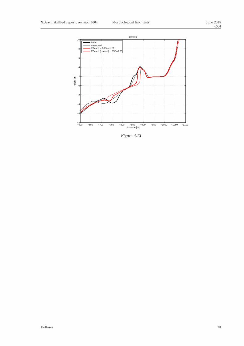
XBeach skillbed report, revision 4664 Morphological field tests June 2015
4664
−1100−1050−1000−950−900−850−800−750−700−650−600−8
−6
−4
−2
0
2
4
6
8
10profiles
distance [m]
heig
ht [m
]
initialmeasuredXBeach − BSS=−1.25XBeach (current) − BSS=0.05
Figure 4.13
Deltares 73

June 2015
4664
Morphological field tests XBeach skillbed report, revision 4664
74 Deltares

XBeach skillbed report, revision 4664 Comparisons with other models June 2015
4664
Chapter 5
Comparisons with other models
In this chapter, XBeach is compared to results obtained from other models. The comparisonsare currently focussed on the DUROS+ and D++ (Vellinga, 1986; Delft Hydraulics, 2006;Deltares, 2010) models that are used for the assessment of dunes along the Dutch coast.Comparisons with other models like DurosTA (Steetzel, 1993) are made throughout the reportand are not discussed specifically in this chapter at the moment.
5.1 Field applications
In this section, DUROS+ (Vellinga, 1986; Delft Hydraulics, 2006) and D++ are (Deltares,2010) compared with XBeach based on field applications. Comparisons are made based onerosion volumes and retreat distances, since these are the main parameters of interest in dunesafety assessment.
5.1.1 Retreat distances JARKUS
In this test, retreat distances obtained from DUROS+ and XBeach using a selection ofJARKUS profiles characteristic for the Dutch coast are compared (Den Heijer et al., 2011).The comparison is presented in Figure 5.1. The retreat distance is defined as the horizontaldistance between the NAP+5m contour and the erosion point. The erosion point is definedas the first diversion point between the pre-storm and post-storm profile, when going fromthe land side in seaward direction. Diversion is considered as a vertical difference of morethan 5cm.
Deltares 75

June 2015
4664
Comparisons with other models XBeach skillbed report, revision 4664
20 40 60 80 100 120 140
20
40
60
80
100
120
140
XBeach retreat distance [m]
DU
RO
S+ r
esp.
D+
+ r
etre
at d
ista
nce
[m]
XBeach vs. DUROS+XBeach vs. D++1:1
Figure 5.1: Scatter plot of retreat distances obtained from XBeach and DUROS+ (bluecircle) and XBeach and D++ (green cross).
76 Deltares

XBeach skillbed report, revision 4664 Specific functionalities June 2015
4664
Chapter 6
Specific functionalities
In the previous chapters, the core functionalities are discussed: hydro- and morphodynamicson different scales. However, XBeach is equipped with a variety of additional functionalitiesthat facilitate more complex computations. One example already discussed is hard elementsin the profiles. This chapter discusses a variety of other functionalities, like discharges, driftersand multiple sediment fractions.
6.1 River outflow
The river outflow case is meant to test XBeach for the combined effects of a river outflowand a steady wave-driven longshore current on the sediment transport and the morphologicalevolution. Though purely hypothetical, this case contains many salient features of real-lifeapplications, such as longshore currents through open side-boundaries and exchange of waterand sand through a gap in a closed boundary. Thus, the formulation of open boundaryconditions is also tested here.
The initial topography consists of a plane beach (slope 1:50), which is interrupted by a 75 mwide river mouth with a water outflow of 150 m3/s. The bottom contours are straight andparallel to the shoreline, except for a shallow submerged channel in line with the river.
The computational grid is rectangular, with 56 nodes in the x-direction (cross-shore) and111 nodes in the y-direction (longshore), with a uniform grid spacing of 15 m. The wavesare irregular and long-crested, with a root-mean-square height of 2m at a water depth of13.5m. The direction of wave incidence is 30 degrees with respect to the shore-normal. Thepeak wave period is 8s. The bed material is uniform sand of 250, with a settling velocity of0.031m/s.
In this figure the bathymetry is shown after approxiately 4 days; arrows indicate the sedimenttransport vectors. plotted for every cross-shore cell and every third longshore cell. Whenfunctioning correctly, we see a channel that has turned towards the north and striaght contourlines downstream of the channel.
Deltares 77

June 2015
4664
Specific functionalities XBeach skillbed report, revision 4664
0200
400600
800
0
200
400
600
800
1000
1200
1400
1600
−10−5
0
−10
−8
−6
−4
−2
0
2
Figure 6.1: Final bathymetry
6.2 Drifters
This purely hypothetical test combines three specific functionalities of XBeach: curvilineargrids, discharges and drifters. The model is basicly an odd-shaped bathtub with a singledischarge location at the left boundary. The bathtub is filled by the discharged water, in-dicated by the increasing water levels (colored background). The bathtub is approximately70m x 70m. Considering that, the discharge of 50m3/s is rather large. Every 10 seconds,two drifters are released just before the discharge opening. One of the two drifters is releasedat the upper boundary of the opening, the other at the lower boundary. The entire path asingle drifter has followed at a certain moment in time is plotted in Figure 6.2. Two largeeddies driven by the large discharge are revealed by these paths.
78 Deltares

XBeach skillbed report, revision 4664 Specific functionalities June 2015
4664
Figure 6.2: Drifter paths after 50, 100, 150 and 450 seconds
6.3 Multiple sediment fractions
The purpose of this simulation is to ensure the multiple sediment fractions model in XBeachperforms as expected. In this test, the Deltaflume 2006 T01 test is recreated with two typesof sand with different colours, red and blue. The sand is initially placed in a zebra-stripepattern in the profile. The properties of both types of sand such as the grain size and mobilityare the same as the sand used in the Deltaflume experiment. For the test to be successful,the following conditions should be met:
1. The simulated final profile should be the same as the final profile in the originalDeltaflume 2006 T01 test.
2. The two sediment types should mix and form layers over each other (yellow).
The figures Figure 6.3 and Figure 6.4 show the initial and final distribution of red and bluesediment in the profile near the dune face. The red and blue lines in the same figure showthe sediment concentration of each sediment type in the water column. If the simulation issuccessful, the red and blue sediment will be well mixed on the foreshore and fresh blue sedi-ment will be deposited over the red sediment at the dune foot as the dune face retreats. Theconcentration of blue sediment in the water column should be higher than the concentrationof red sediment in the water in areas where only blue sediment is available in the top layerof the bed.
The red lines in Figure 6.5 show the predicted dune face retreat and bed level change in theXBeach multiple-sediment model. The black lines in the same figure are the correspondingmeasured profiles. If the simulation has been successful, the red and black lines will alignreasonably well. The results of this simulation should be compared to the Deltaflume 2006T01 test described earlier in this report.
Deltares 79

June 2015
4664
Specific functionalities XBeach skillbed report, revision 4664
Figure 6.3: Initial bathymetry and sediment distribution
Figure 6.4: Final bathymetry and sediment distribution
80 Deltares

XBeach skillbed report, revision 4664 Specific functionalities June 2015
4664
185 190 195 200 205 210 215−1.5
−1
−0.5
0
0.5
1
1.5
2profiles
distance [m]
heig
ht [m
]
initialmeasuredXBeach (current) − BSS=0.88
Figure 6.5: Profile development
6.4 Curvilinear
In this test a curvi-linear grid is applied to simulate waves and hyrdodynamics around avirtual island. The island is circular with a linear sloping profile. The lower half of theoffshore boundary generates bichromatic waves that partly refract towards the island, butalso passes the island. The waves passing the island leave the model through the upper halfof the offshore boundary. Reflections at the offshore boundary are minimal due to the 2Dweakly-reflective boundary condition used (Van Dongeren and Svendsen, 1997).
?? shows the RMS wave height (color) and the flow velocity field (arrows) around the islandin the last time step. ?? shows the same parameters, but in this case the overall mean valuesare presented.
Deltares 81

June 2015
4664
Specific functionalities XBeach skillbed report, revision 4664
Figure 6.6: Snapshot of the RMS wave height and the flow velocity field in the last timestep
Figure 6.7: Mean values of the RMS wave height and the flow velocity field
82 Deltares

XBeach skillbed report, revision 4664 References June 2015
4664
Chapter 7
References
Abdelrahman, S. M. and Thornton, E. B. (1987). Changes in the short wave amplitude andwavenumber due to presence of infragravity waves. In Proceedings Speciality Conferenceon Coastal Hydrodynamics, pages 458–478.
Arcilla, A. S., Roelvink, J. A., O’Connor, B. A., Reniers, A., and Jimenez, J. A. (1994). Thedelta flume ’93 experiment. In Coastal Dynamics, pages 488–502.
Bakkenes, H. J. (2002). Observation and seperation of bound and free low-frequency wavesin the nearshore zone. Master’s thesis, Delft University of Technology.
Birkemeier, W. A., Donoghue, C., Long, C. E., Hathaway, K. K., and Baron, C. F. (1997).1990 delilah nearshore experiment: Summary report. Technical Report CHL-97-4-24, U.S.Army Corps of Engineers. Field Research Facility.
Boers, M. (1996). Simulation of a surf zone with barred beach, part 1: Wave heights andwave breaking. Communications on Hydraulic and Geotechnical Engineering 69-5, DelftUniversity of Technology. 116 p.
Carrier, G. F. and Greenspan, H. P. (1958). Water waves of finite amplitude on a slopingbeach. Journal of Fluid Mechanics, 4:97–109.
Costa, M., Silva, R., and Vitorino, J. (2001). Contribuio para o estudo do clima de agitaomartima na costa portuguesa. In 2as Jornadas Portuguesas de Engenharia Costeira ePorturia, page 20p, Sines. in Portuguese.
Damgaard, J., Dodd, N., Hall, L., and Chesher, R. (2002). Morphodynamic modelling of ripchannel growth. Coastal Engineering, 45:199–221.
Delft Hydraulics (2006). Dune erosion – product 2: Large-scale model tests and dune erosionprediction method. Report H4357, Delft Hydraulics.
Deltares (2010). Ontwikkeling detailtoets duinen 2011. Interim report 1202124-003, Deltares.in Dutch.
Deltares (2011). Validation of dune impact models using european field data. Report 1002266,Deltares.
Den Heijer, C., Walstra, D. J. R., Van Thiel de Vries, J. S. M., Huisman, B. J. A., Hoonhout,B. M., Diermanse, F. L. M., and Van Gelder, P. H. A. J. M. (2011). Importance ofdune erosion influencing processes. Journal of Coastal Research, SI 64(1):283–287. ISSN0749-0208.
Deltares 83

June 2015
4664
References XBeach skillbed report, revision 4664
Dongeren, A. V., Lowe, R., Pomeroy, A., Trang, D. M., Roelvink, D., Symonds, G., andRanasinghe, R. (2013). Numerical modeling of low-frequency wave dynamics over a fringingcoral reef. Coastal Engineering, 73(0):178 – 190.
Erikson, L., Larson, M., and Hanson, H. (2005). Prediction of swash motion and run-upincluding the effects of swash interaction. Coastal Engineering, 52:285–302.
Feddersen, F., Guza, R. T., Elgar, S., and Herbers, T. C. (2000). Velocity moments in along-shore bottom shear stress parameterizations. Journal of Geophysical Research, 105:8673–8688.
Gama, C., Dias, J. A., Ferreira, O., and Taborda, R. (1994). Analysis of storm surge inportugal, between june 1986 and may 1988. In Proceedings Second International Sym-posium on Coastal Zone Research - Management and Planning, pages 381–387, Lisbon.EUROCOAST.
Huntley, D. A., Guza, R. T., and Thornton, E. B. (1981). Field observations of surf beats,1, progressive edge waves. Journal of Geophysical Research, 86:6451–6466.
Jimenez, J. A., Sallenger, A. H., and Fauver, L. (2006). Sediment transport and barrier islandchanges during massive overwash events. In 30th International Conference on CoastalEngineering, San Diego, California, USA. ASCE.
Larson, M., Erikson, L., and Hanson, H. (2004). An analytical model to predict dune erosiondue to wave impact. Coastal Engineering, 51(8–9):675–696.
Leatherman, S. P., Williams, A. T., and Fisher, J. S. (1977). Overwash sedimentation asso-ciated with a large-scale northeaster. Marine Geology, 24:109–121.
List, J. H. (1992). A model for two-dimensional surfbeat. Journal of Geophysical Research,97:5623–5635.
Murphy, A. H. and Epstein, E. S. (1989). Skill scores and correlation coefficients in modelverification. Monthly Whether Review, 117:572–581.
Nairn, R. B., Roelvink, J. A., and Southgate, H. N. (1990). Transition zone width and impli-cations for modelling surfzone hydrodynamics. In Edge, B. L., editor, 22th InternationalConference on Coastal Engineering, pages 68–81, Reston, Virginia, USA. ASCE.
Nishi, R. and Kraus, N. C. (1996). Mechanism and calculation of sand dune erosion ofstorms. In 25th International Conference on Coastal Engineering, pages 3034–3047, Or-lando, Florida, USA. ASCE.
Overton, M. F. and Fisher, J. S. (1988). Laboratory investigation of dune erosion. Journalof Waterway, Port, Coastal and Ocean Engineering, 114(3):367–373.
Ozkan-Haller, H. T. and Kirby, J. T. (1997). A fourier-chebyshev collocation method for theshallow water equations including shoreline runup. Applied Ocean Research, 19:21–34.
Phillips, O. M. (1977). The Dynamics of the Upper Ocean. Cambridge University Press, NewYork, 2nd edition.
Pires, H. O. (1998). Project india, preliminary report on wave climate at faro. Technicalreport, Instituto de Meteorologia, IST, Lisbon.
84 Deltares

XBeach skillbed report, revision 4664 References June 2015
4664
Pomeroy, A., Lowe, R., Symonds, G., Dongeren, A. V., and Moore, C. (2012). The dynamicsof infragravity wave transformation over a fringing reef. Journal of Geophysical Research,117(C11022):1 – 17.
Raubenheimer, B. and Guza, R. T. (1996). Observations and predictions of run-up. Journalof Geophysical Research, 101(C10):25,575–25,587.
Reniers, A. J. H. M., MacMahan, J., Thornton, E. B., and Stanton, T. P. (2006). Modellinginfragravity motions on a rip-channel beach. Coastal Engineering, 53:209–222.
Reniers, A. J. H. M., Roelvink, J. A., and Thornton, E. B. (2004a). Morphodynamic mod-elling of an embayed beach under wave group forcing. Journal of Geophysical Research,109(C01030).
Reniers, A. J. H. M., Thomas, E. B., Stanton, T. P., and Roelvink, J. A. (2004b). Vertical flowstructure during sandy duck: observations and modeling. Coastal Engineering, 51(3):237–260.
Roelvink, J. A. (1993a). Dissipation in random wave groups incident on a beach. CoastalEngineering, 19:127–150.
Roelvink, J. A. (1993b). Surf beat and its effect on cross-shore profiles. PhD thesis, DelftUniversity of Technology.
Roelvink, J. A., Reniers, A. J. H. M., Van Dongeren, A. R., Van Thiel de Vries, J. S. M.,McCall, R. T., and Lescinski, J. M. (2009). Modelling storm impacts on beaches, dunesand barrier islands. Coastal Engineering, 56(11-12):1133–1152.
Roelvink, J. A. and Stive, M. J. F. (1989). Bar-generating cross-shore flow mechanisms on abeach. Journal of Geophysical Research, 94(C4):4785–4800.
Roelvink, J. A., Van Kessel, T., Alfageme, S., and Canizares, R. (2003). Modelling of barrierisland response to storms. In Coastal Sediments ’03, Clearwater, Florida, USA.
Ruessink, B. G., Miles, J. R., Feddersen, F., Guza, R. T., and Elgar, S. (2001). Modeling thealongshore current on barred beaches. Journal of Geophysical Research, 106:22,451–22,462.
Sallenger, A. H. (2000). Storm impact scale for barrier islands. Journal of Coastal Research,16(3):860–895.
Schaeffer, H. A. (1994). Edge waves forced by short-wave groups. Journal of Fluid Mechanics,259:125–148.
Soulsby, R. L. (1997). Dynamics of Marine Sands. Thomas Telford, London.
Soulsby, R. L., Hamm, L., Klopman, G., Myrhaug, D., Simons, R. R., and Thomas, G. P.(1993). Wavecurrent interaction within and outside the bottom boundary layer. CoastalEngineering, 21:41–69.
Steetzel, H. J. (1987). Systematic research on the effectiveness of dune toe revetments - largescale model investigation. Technical Report H298-I, Delft Hydraulics.
Steetzel, H. J. (1993). Cross-shore transport during storm surges. PhD thesis, Delft Universityof Technology.
Deltares 85

June 2015
4664
References XBeach skillbed report, revision 4664
Stelling, G. S. and Duinmeijer, S. P. A. (2003). A staggered conservative scheme for everyfroude number in rapidly varied shallow water flows. International Journal for NumericalMethods in Fluids, 43:1329–1354.
Stive, M. J. F. and De Vriend, H. J. (1994). Shear stresses and mean flow in shoalingand breaking waves. In Edge, B. L., editor, 24th International Conference on CoastalEngineering, pages 594–608, Reston, Virginia, USA. ASCE.
Stockdon, H. F., Holman, R. A., Howd, P. A., and Sallenger, A. H. (2006). Empiricalparameterization of setup, swash, and runup. Coastal Engineering, 53:573–588.
Sutherland, J., Peet, A. H., and Soulsby, R. L. (2004). Evaluating the performance of mor-phological models. Coastal Engineering, 51(8–9):917–939.
Svendsen, I. A. (1984). Wave heights and set-up in a surf-zone. Coastal Engineering, 8:303–329.
Thornton, E. B., MacMahan, J., and Sallenger, A. H. (2007). Rip currents, mega-cusps, anderoding dunes. Marine Geology, 240(1–4):151–167.
Tucker, M. J. (1954). Surfbeats: sea waves of 1 to 5minutes’ period. In Proceedings of RoyalSociety, number A in 202, pages 565–576, London.
Van de Graaff, J. (1976). Scale series dune erosion. Technical Report M1263 part I, DelftHydraulics. in Dutch.
Van der Werf, J., Van Santen, R., Van Ormondt, M., Briere, C., and Van Dongeren, A. (2011).Operational model to simulate storm impact along the holland coast. In Proceedings CoastalSediments 2011, Miami, Florida, USA.
Van der Werf, J. J. and Van Santen, R. (2010). Operational model to simulate storm im-pact along the holland coast: system development and test application. Technical report,Deltares, Alkyon and Arcadis.
Van Dongeren, A. R., Reniers, A. J. H. M., Battjes, J. A., and Svendsen, I. A. (2003).Numerical modeling of infragravity wave response during delilah. Journal of GeophysicalResearch, 108(C9):3288.
Van Dongeren, A. R. and Svendsen, I. A. (1997). Absorbing-generating boundary conditionfor shallow water models. Journal of Waterway, Port, Coastal and Ocean Engineering,pages 303–313.
Van Gent, M. R. A., Van Thiel de Vries, J. S. M., Coeveld, E. M., De Vroeg, J. H., andVan de Graaff, J. (2008). Large-scale dune erosion tests to study the influence of waveperiods. Coastal Engineering, 55(12).
Van Rijn, L. C., Walstra, D. J. R., Grasmeijer, B., Sutherland, J., Pan, S., and Sierra, J. P.(2003). The predictability of cross-shore bed evolution of sandy beaches at the time scale ofstorms and seasons using process-based profile models. Coastal Engineering, 47(3):295–327.ISSN 0378-3839.
Van Thiel de Vries, J. S. M. (2009). Dune erosion during storm surges. PhD thesis, DelftUniversity of Technology.
Van Thiel de Vries, J. S. M., Van Gent, M. R. A., Walstra, D. J. R., and Reniers, A. J.H. M. (2008). Analysis of dune erosion processes in large-scale flume experiments. CoastalEngineering, 55(12).
86 Deltares

XBeach skillbed report, revision 4664 References June 2015
4664
Vellinga, P. (1981). Scale series dune erosion. Technical Report M1263 part II, Delft Hy-draulics. in Dutch.
Vellinga, P. (1984). Scale series dune erosion: Large scale tests in deltaflume. TechnicalReport M1263 part III, Delft Hydraulics. in Dutch.
Vellinga, P. (1986). Beach and Dune Erosion during Storm Surges. PhD thesis, Delft Uni-versity of Technology.
Visser, P. J. (1998). Breach growth in sand dikes. PhD thesis, Delft University of Technology.
Wang, P. and Horwitz, M. H. (2007). Erosional and depositional characteristics of regionaloverwash deposits caused by multiple hurricanes. Sedimentology, 54:545–564.
Zelt, J. A. (1986). Tsunamis: the response of harbours with sloping boundaries to longwave excitation. PhD thesis, W.M. Keck Laboratory of Hydraulics and Water Resources,Division of Engineering and Applied Science, California Institute of Technology. 318 p.
Deltares 87

June 2015
4664
References XBeach skillbed report, revision 4664
88 Deltares

XBeach skillbed report, revision 4664 Model Performance Statistics June 2015
4664
Appendix A
Model Performance Statistics
A.1 Introduction
In this Appendix the theory behind the Model Performance Statistics (MPS) used in theXBeach skillbed is explained. The MPS are used to quantify the performance of modelresults based on a comparison with measurement data. Different MPS parameters are usedas each parameter has its own characteristics.
First an overview is given of the MPS parameters used in the XBeach skillbed, summarizedin table form including some basic characteristics. Consequently, each MPS parameters listedin the overview table is further explained in separate sections.
A.2 MPS parameters
An overview of the MPS parameters used in the XBeach skillbed is given in Table A.1.
Table A.1: MPS parameters
Parameter Description Ranges
ME & STD Mean Error & Standard Deviation 0: perfect predictionR Correlation coefficient (range: [0 1]) 1: perfect correlationRel. bias Systematic error relative to the mean low value: good performanceSci Scatter Index low values: performanceBSS Brier Skill Score (Sutherland et al., 2004) see belowBSS Brier Skill Score (Murphy and Epstein, 1989) see below
Each parameter listed in the table is further explained in the following paragraphs.
Deltares 89

June 2015
4664
Model Performance Statistics XBeach skillbed report, revision 4664
A.3 Mean Error & Standard Deviation
The Mean Error (ME) and the Standard Deviation (STD) of the error of a time series are auseful measure to quantify model performance for parameters such as wave heights or waterlevels. The SD is in general not so useful when applied to morphological parameters such asthe bed level evolution.
ME =1
N
N∑i=1
(fcomp.,i − fmeas.,i) (A.1)
STD =
√√√√ 1
N − 1
N∑i=2
(fcomp.,i − fmeas.,i −ME)2 (A.2)
A.4 Correlation coefficient
The Correlation Coefficient R is a measure quantifying the correlation of the measurementsand simulation results, but does not indicate significance because the distributions of theseries are not taken into account.
A.5 Relative Bias
The Relative Bias (Rel. Bias) is the systematic error relative to the mean. Relative lowvalues of the mean can cause high vales of the Rel. Bias.
Rel.Bias =
∑Ni=1(fcomp.,i − fmeas.,i)∑N
i=1 fmeas.(A.3)
A.6 Scatter Index
The Scatter index (Sci) is the standard deviation relative to the mean value of the measuredsignal. Relative low values of the mean can cause high vales of the Sci.
Sci =
√1
N−1
∑Ni=2(fcomp.,i − fmeas.,i −ME)2
fmeas.(A.4)
A.7 Brier Skill Score
The Brier Skill Score (BSS) calculates the performance of the performance relative to abaseline prediction. The BSS calculates the mean square difference between the prediction
90 Deltares
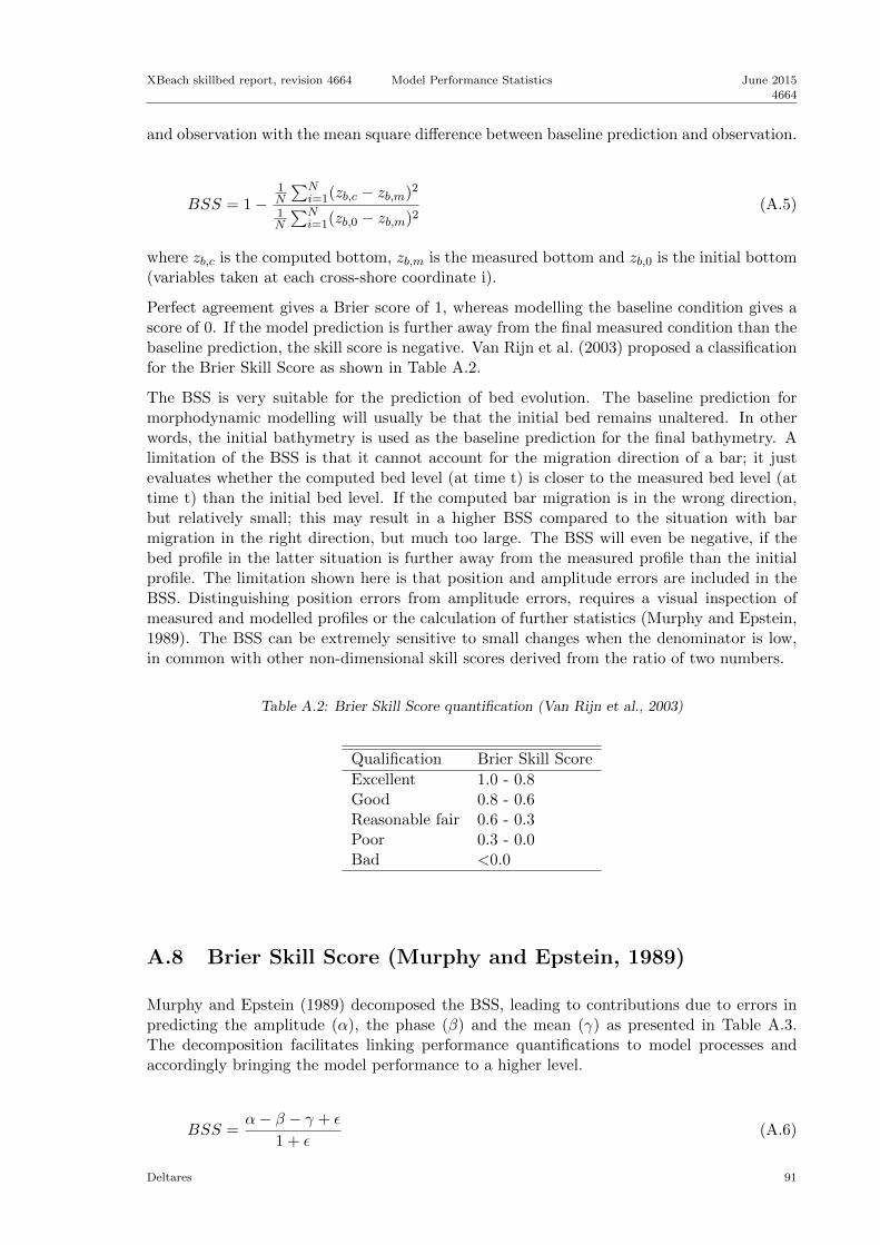
XBeach skillbed report, revision 4664 Model Performance Statistics June 2015
4664
and observation with the mean square difference between baseline prediction and observation.
BSS = 1−1N
∑Ni=1(zb,c − zb,m)2
1N
∑Ni=1(zb,0 − zb,m)2
(A.5)
where zb,c is the computed bottom, zb,m is the measured bottom and zb,0 is the initial bottom(variables taken at each cross-shore coordinate i).
Perfect agreement gives a Brier score of 1, whereas modelling the baseline condition gives ascore of 0. If the model prediction is further away from the final measured condition than thebaseline prediction, the skill score is negative. Van Rijn et al. (2003) proposed a classificationfor the Brier Skill Score as shown in Table A.2.
The BSS is very suitable for the prediction of bed evolution. The baseline prediction formorphodynamic modelling will usually be that the initial bed remains unaltered. In otherwords, the initial bathymetry is used as the baseline prediction for the final bathymetry. Alimitation of the BSS is that it cannot account for the migration direction of a bar; it justevaluates whether the computed bed level (at time t) is closer to the measured bed level (attime t) than the initial bed level. If the computed bar migration is in the wrong direction,but relatively small; this may result in a higher BSS compared to the situation with barmigration in the right direction, but much too large. The BSS will even be negative, if thebed profile in the latter situation is further away from the measured profile than the initialprofile. The limitation shown here is that position and amplitude errors are included in theBSS. Distinguishing position errors from amplitude errors, requires a visual inspection ofmeasured and modelled profiles or the calculation of further statistics (Murphy and Epstein,1989). The BSS can be extremely sensitive to small changes when the denominator is low,in common with other non-dimensional skill scores derived from the ratio of two numbers.
Table A.2: Brier Skill Score quantification (Van Rijn et al., 2003)
Qualification Brier Skill Score
Excellent 1.0 - 0.8Good 0.8 - 0.6Reasonable fair 0.6 - 0.3Poor 0.3 - 0.0Bad <0.0
A.8 Brier Skill Score (Murphy and Epstein, 1989)
Murphy and Epstein (1989) decomposed the BSS, leading to contributions due to errors inpredicting the amplitude (α), the phase (β) and the mean (γ) as presented in Table A.3.The decomposition facilitates linking performance quantifications to model processes andaccordingly bringing the model performance to a higher level.
BSS =α− β − γ + ε
1 + ε(A.6)
Deltares 91

June 2015
4664
Model Performance Statistics XBeach skillbed report, revision 4664
α = r2Y ′X′ ;β = (rY ′X′ − σY ′
σX′)2; γ = (
<Y ′>−<X ′>σX′
)2; ε =<X ′>
σX′
2
(A.7)
Table A.3: Brier Skill Score decomposition factors (Murphy and Epstein, 1989)
Factor Indication Perfect modelling
phase error (α) transport locations α = 1amplitude error (β) transport volumes β = 0map mean error (γ) - γ = 0normalization term (ε) - -
Van Rijn et al. (2003) also proposed a classification for the decomposed Brier Skill Score asshown in Table A.4.
Table A.4: Brier Skill Score (Murphy and Epstein, 1989) quantification (Van Rijn et al.,2003)
Qualification Brier Skill Score
Excellent 1.0 - 0.5Good 0.5 - 0.2Reasonable fair 0.2 - 0.1Poor 0.1 - 0.0Bad <0.0
92 Deltares

XBeach skillbed report, revision 4664 Overview June 2015
4664
Appendix B
Overview
In the table below, the statuses of all tests found in the skillbed are summarized. Thefirst three colomns identify the test with a combination of a binary, test and run name.The following three columns provide information on the status of that specific run. Thesecolumns indicate whether the model ran, the analysis ended succesfully and whether the runused default or custom settings. An empty status means the run or analysis is ignored, across indicates failure and a checkmark indicates success. The other columns in the tableprovide information on the model configuration.
Tests can be run multiple times using different settings. Different runs are identified by arun name, which follows after the test name. If a test runs once only, it is common use toname the run default. This is not the same as running a test with default settings, which isindicated in the “Default settings” column.
The table provides all tests ran in a single skillbed run. This report not necessarily uses allavailable tests. Therefore, not all tests in the table are necessarily found in the continuationof this report.
Table B.1: Status overview skillbed tests
Test Run Sta
tus
Mat
lab
Def
au
ltse
ttin
gs
Con
figu
rati
on
Wav
es*
Wate
rle
vels
**
Fra
ctio
ns
Mor
ph
ology
Hard
layer
s
Gro
un
dw
ater
flow
1953 storm surge default 3 3 1D WG V 1 3
1976 storm surge raai3400 3 3 1D WG V 1 3
1976 storm surge raai568 3 3 1D WG V 1 3
1976 storm surge raai6050 3 3 1D WG V 1 3
Assateague Island profA 3 3 1D ST C 1 3
Assateague Island profB1 3 3 1D ST C 1 3
Assateague Island profB2 3 3 1D ST C 1 3
Assateague Island profC 3 3 1D ST C 1 3
Boers 1C custom 3 3 1D WG C 1Boers 1C default 3 3 1D WG C 1CarrierGreenspan default 3 3 1D ST C 1Curvi Island default 3 3 2D WG C 1
Deltares 93

June 2015
4664
Overview XBeach skillbed report, revision 4664
Table B.1: Status overview skillbed tests
Test Run Sta
tus
Matl
ab
Def
au
ltse
ttin
gs
Con
figu
rati
on
Wav
es*
Wate
rle
vels
**
Fra
ctio
ns
Morp
holo
gy
Har
dla
yer
s
Gro
un
dw
ater
flow
DUROS refere... 3 3 1D WG C 1 3
DUROS transe... 3 3 1D WG C 1 3
DUROS transe... 3 3 1D WG C 1 3
DUROS transe... 3 3 1D WG C 1 3
DUROS transe... 3 3 1D WG C 1 3
DUROS transe... 3 3 1D WG C 1 3
DUROS transe... 3 3 1D WG C 1 3
DUROS transe... 3 3 1D WG C 1 3
DUROS transe... 3 3 1D WG C 1 3
DUROS transe... 3 3 1D WG C 1 3
DUROS transe... 3 3 1D WG C 1 3
DUROS transe... 3 3 1D WG C 1 3
DUROS transe... 3 3 1D WG C 1 3
DUROS transe... 3 3 1D WG C 1 3
DUROS transe... 3 3 1D WG C 1 3
DUROS transe... 3 3 1D WG C 1 3
DUROS transe... 3 3 1D WG C 1 3
DUROS transe... 3 3 1D WG C 1 3
DUROS transe... 3 3 1D WG C 1 3
DUROS transe... 3 3 1D WG C 1 3
DUROS transe... 3 3 1D WG C 1 3
DUROS transe... 3 3 1D WG C 1 3
DUROS transe... 3 3 1D WG C 1 3
DUROS transe... 3 3 1D WG C 1 3
DUROS transe... 3 3 1D WG C 1 3
Delilah 199010131000 default 3 3 2D WG C 1Deltaflume2006 DP01 3 3 1D WG C 2 3
Deltaflume2006 DP02 3 3 1D WG C 2 3
Deltaflume2006 T01 3 3 1D WG C 2 3
Deltaflume2006 T01 zebra 3 7 1D WG C 2 3
Deltaflume2006 T02 3 3 1D WG C 2 3
Deltaflume2006 T03 3 3 1D WG C 2 3
Deltaflume2006 T04 3 3 1D WG C 2 3
DeltaflumeH298 T1 3 3 1D WG C 1 3 3
DeltaflumeH298 T2 3 3 1D WG C 1 3 3
DeltaflumeH298 T3 3 3 1D WG C 1 3 3
DeltaflumeLIP11D 1B 3 3 1D WG C 1 3
DeltaflumeLIP11D 1C 3 3 1D WG C 1 3
DeltaflumeLIP11D 2E 3 3 1D WG C 1 3
Deltaflume H4731 T11 3 3 1D WG C 1 3 3
Deltaflume H4731 T12 3 3 1D WG C 1 3 3
Deltaflume H4731 T14 3 3 1D WG C 1 3 3
94 Deltares

XBeach skillbed report, revision 4664 Overview June 2015
4664
Table B.1: Status overview skillbed tests
Test Run Sta
tus
Matl
ab
Def
au
ltse
ttin
gs
Con
figu
rati
on
Wav
es*
Wate
rle
vels
**
Fra
ctio
ns
Morp
hol
ogy
Har
dla
yer
s
Gro
un
dw
ater
flow
Deltaflume M1263 III Test-1 3 3 1D WG C 1 3
Deltaflume M1263 III Test-2 3 3 1D WG C 1 3
Deltaflume M1263 III Test-3 3 3 1D WG C 1 3
Deltaflume M1263 III Test-4 3 3 1D WG C 1 3
Deltaflume M1263 III Test-5 3 3 1D WG C 1 3
Deltaflume M1797 T01 3 3 1D WG V 1 3
Deltaflume M1797 T02 3 3 1D WG V 1 3
Drifters default 3 3 2D ? C 1GWK86 T01 3 3 1D WG V 1 3
GWK86 T02 3 3 1D WG V 1 3
GWK86 T03 3 3 1D WG V 1 3
GWK86 T04 3 3 1D WG V 1 3
GWK86 T05 3 3 1D WG V 1 3
GWK86 T06 3 3 1D WG V 1 3
GWK98 A9 3 3 1D WG C 1 3
GWK98 B2 3 3 1D WG C 1 3
GWK98 C2 3 3 1D WG C 1 3
GWK98 F1 3 3 1D WG C 1 3
GWK98 H2 3 3 1D WG C 1 3
MICORE Cadiz Urb... north 3 3 1D WG V 1 3
MICORE Dziwnow Spit 386 3 3 1D WG V 1 3
MICORE Kamchia S... pr04 3 3 1D WG V 1 3
MICORE Lido di Dante mar201... 3 3 1D WG V 1 3
MICORE Mariakerk... s116a 3 3 1D WG V 1 3 3
MICORE Praia de Faro event9 3 3 1D WG V 1 3
Netcdf default 7 3 1D ST C 1Ningaloo reef default 3 3 1D WG V 1 3
River Outflow default 3 3 2D ST C 1 3
Scheldtflume H4265 T01 3 3 1D WG C 1 3
Scheldtflume H4265 T02 3 3 1D WG C 1 3
Scheldtflume H4265 T02a 3 3 1D WG C 1 3
Scheldtflume H4265 T03 3 3 1D WG C 1 3
Scheldtflume H4265 T11 3 3 1D WG C 1 3
Scheldtflume H4265 T12 3 3 1D WG C 1 3
Scheldtflume H4265 T13 3 3 1D WG C 1 3
Scheldtflume M1819 I T01 3 3 1D WG V 1 3
Scheldtflume M1819 I T02 3 3 1D WG V 1 3
Scheldtflume M1819 I T03 3 3 1D WG V 1 3
Scheldtflume M1819 I T04 3 3 1D WG V 1 3
Scheldtflume M1819 I T05 3 3 1D WG V 1 3
Scheldtflume M1819 I T06 3 3 1D WG V 1 3
Scheldtflume M1819 I T07 3 3 1D WG V 1 3
Deltares 95

June 2015
4664
Overview XBeach skillbed report, revision 4664
Table B.1: Status overview skillbed tests
Test Run Sta
tus
Matl
ab
Def
au
ltse
ttin
gs
Con
figu
rati
on
Wav
es*
Wate
rle
vels
**
Fra
ctio
ns
Morp
holo
gy
Har
dla
yer
s
Gro
un
dw
ater
flow
Scheldtflume M1819 I T08 3 3 1D WG V 1 3
Scheldtflume M1819 I T09 3 3 1D WG V 1 3
Scheldtflume M1819 I T10 3 3 1D WG V 1 3
Scheldtflume M1819 I T11 3 3 1D WG V 1 3
Scheldtflume M1819 I T12 3 3 1D WG V 1 3
Scheldtflume M1819 I T13 3 3 1D WG V 1 3
Scheldtflume M1819 I T14 3 3 1D WG V 1 3
Scheldtflume M1819 I T21 3 3 1D WG V 1 3
Scheldtflume M1819 I T22 3 3 1D WG V 1 3
Scheldtflume M1819 I T23 3 3 1D WG V 1 3
Scheldtflume M1819 I T24 3 3 1D WG V 1 3
Scheldtflume M1819 I T25 3 3 1D WG V 1 3
Scheldtflume M1819 I T26 3 3 1D WG V 1 3
Scheldtflume M1819 I T27 3 3 1D WG V 1 3
Scheldtflume M1819 I T28 3 3 1D WG V 1 3
Scheldtflume M1819 I T29 3 3 1D WG V 1 3
Scheldtflume M18... T01 3 3 1D WG V 1 3 3
Scheldtflume M18... T02 3 3 1D WG V 1 3 3
Scheldtflume M18... T03 3 3 1D WG V 1 3 3
Scheldtflume M18... T04 3 3 1D WG V 1 3 3
Windflume M1263 I AT33 3 3 1D WG C 1 3
Windflume M1263 I AT47 3 3 1D WG C 1 3
Windflume M1263 I AT61 3 3 1D WG C 1 3
Windflume M1263 I AT71 3 3 1D WG C 1 3
Windflume M1263 I AT91 3 3 1D WG C 1 3
Windflume M1263 I AT95 3 3 1D WG C 1 3
Windflume M1263 I BT13 3 3 1D WG C 1 3
Windflume M1263 I BT15 3 3 1D WG C 1 3
Windflume M1263 I BT17 3 3 1D WG C 1 3
Windflume M1263 I BT23 3 3 1D WG C 1 3
Windflume M1263 I BT25 3 3 1D WG C 1 3
Windflume M1263 I BT27 3 3 1D WG C 1 3
Windflume M1263 I BT45 3 3 1D WG C 1 3
Windflume M1263 I BT62 3 3 1D WG C 1 3
Windflume M1263 I BT72 3 3 1D WG C 1 3
Windflume M1263 I BT92 3 3 1D WG C 1 3
Windflume M1263 I BT96 3 3 1D WG C 1 3
Windflume M1263 I CT14 3 3 1D WG C 1 3
Windflume M1263 I CT16 3 3 1D WG C 1 3
Windflume M1263 I CT18 3 3 1D WG C 1 3
Windflume M1263 I CT24 3 3 1D WG C 1 3
Windflume M1263 I CT26 3 3 1D WG C 1 3
96 Deltares

XBeach skillbed report, revision 4664 Overview June 2015
4664
Table B.1: Status overview skillbed tests
Test Run Sta
tus
Matl
ab
Def
au
ltse
ttin
gs
Con
figu
rati
on
Wav
es*
Wate
rle
vels
**
Fra
ctio
ns
Morp
hol
ogy
Har
dla
yer
s
Gro
un
dw
ater
flow
Windflume M1263 I CT28 3 3 1D WG C 1 3
Windflume M1263 I CT46 3 3 1D WG C 1 3
Windflume M1263 I CT63 3 3 1D WG C 1 3
Windflume M1263 I CT73 3 3 1D WG C 1 3
Windflume M1263 I CT93 3 3 1D WG C 1 3
Windflume M1263 I CT97 3 3 1D WG C 1 3
Windflume M1263 I DT34 3 3 1D WG C 1 3
Windflume M1263 I DT48 3 3 1D WG C 1 3
Windflume M1263 I DT64 3 3 1D WG C 1 3
Windflume M1263 I DT74 3 3 1D WG C 1 3
Windflume M1263 I DT94 3 3 1D WG C 1 3
Windflume M1263 I DT98 3 3 1D WG C 1 3
Windflume M1263 II 101 3 3 1D WG C 1 3
Windflume M1263 II 105 3 3 1D WG C 1 3
Windflume M1263 II 111 3 3 1D WG C 1 3
Windflume M1263 II 115 3 3 1D WG C 1 3
Windflume M1263 II 121 3 3 1D WG C 1 3
Windflume M1263 II 122 3 3 1D WG C 1 3
Windflume M1263 II 123 3 3 1D WG C 1 3
Windflume M1263 II 124 3 3 1D WG C 1 3
Windflume M1263 II 125 3 3 1D WG C 1 3
Windflume M1263 II 126 3 3 1D WG C 1 3
Windflume M1263 II 127 3 3 1D WG C 1 3
Windflume M1263 II 128 3 3 1D WG C 1 3
Zelt Case1 default 3 3 2D WG C 1Zwin T01 default 3 3 2D ST V 1 3
long wave propag... default 3 3 1D ST C 1longcrested refr... 1bin a... 3 3 2D WG C 1longcrested refr... 1bin a... 3 3 2D WG C 1longcrested refr... 1bin a... 3 3 2D WG C 1longcrested refr... 3bin a... 3 3 2D WG C 1longcrested refr... 3bin a... 3 3 2D WG C 1longcrested refr... 3bin a... 3 3 2D WG C 1longcrested refr... 5bin a... 3 3 2D WG C 1longcrested refr... 5bin a... 3 3 2D WG C 1longcrested refr... 5bin a... 3 3 2D WG C 1longcrested refr... 10deg 3 3 1D ST C 1longcrested refr... 2p5deg 3 3 1D ST C 1longcrested refr... 5deg 3 3 1D ST C 1longcrested refr... snellius 3 3 1D ST C 1tideonly blanke... 3 3 2D ST V 1tideonly default 3 3 2D ST V 1
Deltares 97

June 2015
4664
Overview XBeach skillbed report, revision 4664
Table B.1: Status overview skillbed tests
Test Run Sta
tus
Matl
ab
Def
au
ltse
ttin
gs
Con
figu
rati
on
Wav
es*
Wate
rle
vels
**
Fra
ctio
ns
Morp
holo
gy
Har
dla
yer
s
Gro
un
dw
ater
flow
* ST = stationary, WG = wave groups, NH = non-hydrostatic** C = constant, V = varying
98 Deltares