XFUNC - Inicial — UFRGS XFUNC.pdf · The purpose of the program XFUNC is to compute the frequency domain transfer function of a circuit in symbolic format, given a circuit description

XFUNC

SYMBOLIC CIRCUIT ANALYSIS

SOFTWARE

VERSION 2.1

Copyright © 1993, YY Software

XFUNC 2.1 --------------------------------------------------------------------

--------------------------------------------------------------------


i

TABLE OF CONTENT I. INTRODUCTION..........................................Page 1 1. PURPOSE.........................................Page 1 2. WHAT IS UNIQUE ABOUT XFUNC......................Page 1 3. FEATURES........................................Page 2 4. ACKNOWLEDGEMENT.................................Page 3 5. TRADEMARKS......................................Page 4 II. INSTALLATION..........................................Page 5 1. HARDWARE AND SOFTWARE REQUIREMENTS..............Page 5 2. INSTALLATION....................................Page 6 III. PROGRAM OPERATION.....................................Page 7 1. INTEGRATED ENVIRONMENT..........................Page 7 About - Information.............................Page 7 About - Program.................................Page 7 About - Register................................Page 7 File - File Name................................Page 7 File - Edit Circuit.............................Page 8 File - View Output..............................Page 8 File - Configure................................Page 8 File - DOS Command..............................Page 9 File - DOS Shell................................Page 9 File - Quit.....................................Page 9 Analysis - Go..................................Page 10 Data - ........................................Page 10 Data - Load....................................Page 10 Data - Save....................................Page 10 Data - Window..................................Page 10 Data - Modify..................................Page 11 Sign Change..............................Page 11 Inverse..................................Page 11 Add by...................................Page 11 Subtract by..............................Page 11 Multiply by..............................Page 11 Divide by................................Page 11 Substitute...............................Page 11 Data - f-t Transform...........................Page 11 Initial Value............................Page 12 Final Value..............................Page 12 Laplace,Z Transform......................Page 12

XFUNC 2.1 --------------------------------------------------------------------

-------------------------------------------------------------------- Copyright © 1993, YY Software

ii

Data - S-Z Transform...........................Page 14 Forward Derivative.......................Page 15 Backward Derivative......................Page 15 Bilinear.................................Page 15 Impulse Invariant........................Page 16 Data - Undo....................................Page 16 Plot - ........................................Page 16 Plot - Gain-Phase..............................Page 16 Plot - Bode....................................Page 17 Plot - Pole-Zero...............................Page 17 Plot - Nyquist.................................Page 17 Plot - Impulse.................................Page 18 Plot - Step....................................Page 18 F1=Help........................................Page 18 2. DOS COMMAND LINE ENVIRONMENT...................Page 19 IV. WRITING A CIRCUIT FILE...............................Page 20 1. COMMENT........................................Page 21 2. CIRCUIT TITLE..................................Page 21 3. USER OPTION....................................Page 22 4. ANALYSIS MODE..................................Page 24 5. INPUT SOURCE...................................Page 25 6. OUTPUT METER...................................Page 26 7. PASSIVE COMPONENT..............................Page 27 8. LINEAR DEPENDENT SOURCE........................Page 29 9. IDEAL OPAMP....................................Page 31 10. SWITCH.........................................Page 32 11. TIME INTERVAL DECLARATION......................Page 33 12. END LINE.......................................Page 34 APPENDIX A: APPLICATION NOTES..............................App A-1 I. MODELING COMPONENTS..................................App A-2 1. LINEAR TRANSFORMERS............................App A-2 2. LOSSLESS TRANSMISSION LINES....................App A-3 II. FILES TRANSFER DIAGRAM...............................App A-4 III. LINEAR CIRCUIT ANALYSIS TECHNIQUES...................App A-7 1. INPUT AND OUTPUT IMPEDANCES....................App A-7 2. LINEAR CIRCUIT EQUATIONS.......................App A-7

XFUNC 2.1 --------------------------------------------------------------------

--------------------------------------------------------------------


iii

IV. SWITCHING CIRCUIT ANALYSIS TECHNIQUES................App A-9 1. STATE SPACE AVERAGING..........................App A-9 2. STATE CHANGE CALCULATION......................App A-11 V. ERRORS AND PROBLEMS.................................App A-14 1. ERROR CODES...................................App A-14 A. SHELL.EXE Errors........................App A-14 B. ANALYSIS.EXE Errors.....................App A-16 C. OPERATE.EXE Errors......................App A-19 2. AVOIDING PROBLEMS AND ERRORS..................App A-23 3. EXISTING PROBLEMS AND BUGS....................App A-27 VI. OPTIMIZING THE RESULTS..............................App A-28 1. ANALYSIS.EXE CALCULATIONS.....................App A-28 2. OPERATE.EXE CALCULATIONS......................App A-31 VII. FURTHER IMPROVEMENTS................................App A-33 END OF DOCUMENT................................................ X

XFUNC 2.1 --------------------------------------------------------------------

--------------------------------------------------------------------


Page 1

I. INTRODUCTION 1. PURPOSE The purpose of the program XFUNC is to compute the frequency

domain transfer function of a circuit in symbolic format, given a circuit description netlist in linear model. In addition to this basic feature, the program provides various extras, which will be discussed in the following sections.

2. WHAT IS UNIQUE ABOUT XFUNC Electronic Engineers, Research Scientists, or Mathematician

will find XFUNC most useful. Most circuit analysis software such as SPICE on the market

today only give numerical frequency response solution to a given circuit. But it is sometimes necessary to find out the frequency response with respect to various circuit parameters, and to choose component values to optimize the performance. The most direct and proven way to achieve these is to generate the mathematical transfer function description of the circuit. XFUNC saves the Engineer's time and tedious efforts to generate the symbolic mathematical transfer function.

Another important feature of XFUNC as compared to most other

circuit analysis software is its ability to use state-space averaging technique to analysis a switching circuit. Although SPICE based programs can calculate transient response, they do not provide frequency response solution to a switching circuit. It should be noted that because XFUNC is symbolic based, it is not designed to handle large circuits. For most analog circuit analysis, it is best to break up a large circuit into small blocks to analyze each block.

In addition to circuit analysis, XFUNC can be used as a

simple tools for symbolic algebra. Besides addition, multiplication, etc, it can be used as a symbolic matrix

XFUNC 2.1 --------------------------------------------------------------------


Page 2

simplifier and solver. It also generates plots for the results.

XFUNC 2.1 --------------------------------------------------------------------

--------------------------------------------------------------------


Page 3

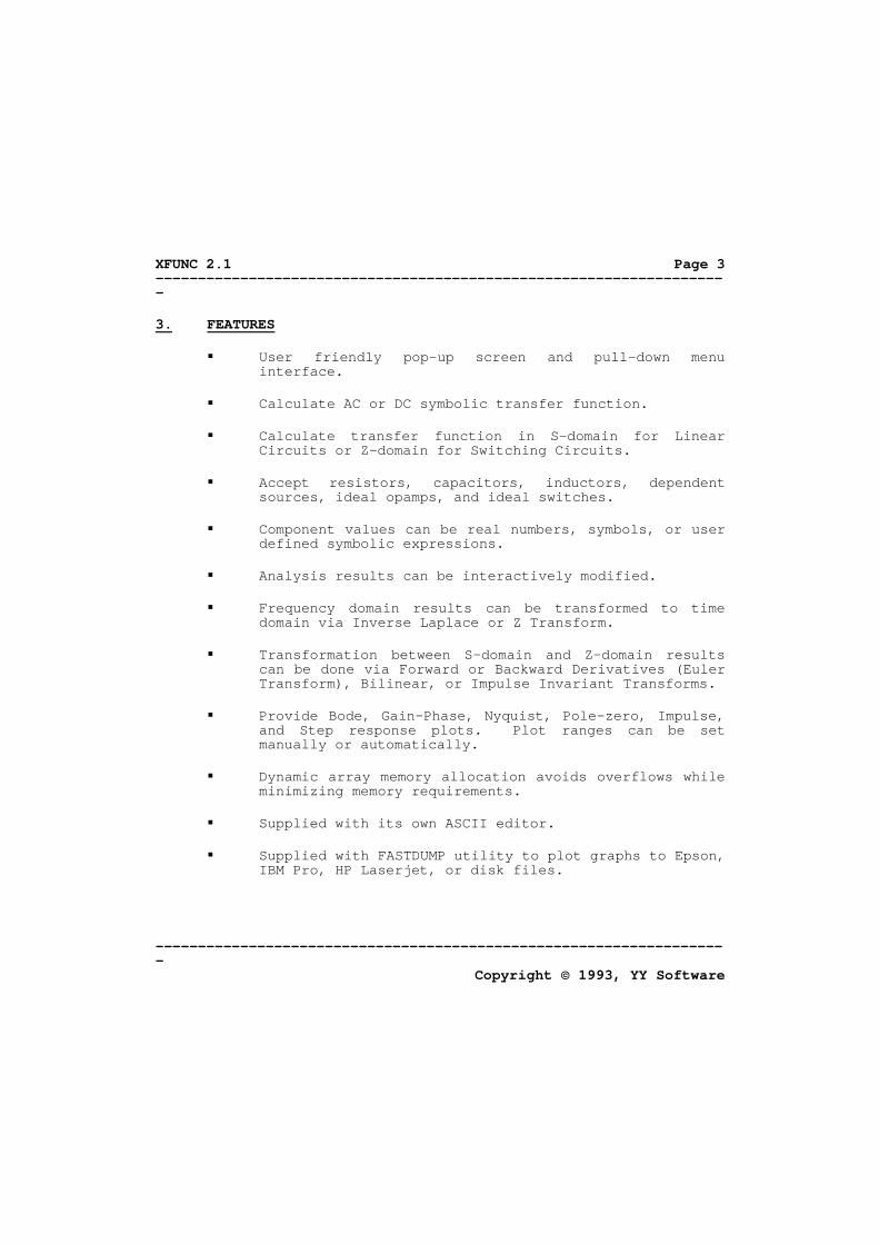
3. FEATURES User friendly pop-up screen and pull-down menu

interface. Calculate AC or DC symbolic transfer function. Calculate transfer function in S-domain for Linear

Circuits or Z-domain for Switching Circuits. Accept resistors, capacitors, inductors, dependent

sources, ideal opamps, and ideal switches. Component values can be real numbers, symbols, or user

defined symbolic expressions. Analysis results can be interactively modified. Frequency domain results can be transformed to time

domain via Inverse Laplace or Z Transform. Transformation between S-domain and Z-domain results

can be done via Forward or Backward Derivatives (Euler Transform), Bilinear, or Impulse Invariant Transforms.

Provide Bode, Gain-Phase, Nyquist, Pole-zero, Impulse,

and Step response plots. Plot ranges can be set manually or automatically.

Dynamic array memory allocation avoids overflows while

minimizing memory requirements. Supplied with its own ASCII editor. Supplied with FASTDUMP utility to plot graphs to Epson,

IBM Pro, HP Laserjet, or disk files.

XFUNC 2.1 --------------------------------------------------------------------


Page 4

4. ACKNOWLEDGEMENT This section provides information on how the XFUNC Symbolic

Circuit Analysis Software Version 2.1 was developed. These references are so important to the development of this program not to mention first. Without them, XFUNC would never have existed. For those who are only interested in how to use this program, skip this section.

A. Software Development Tools Compiler: Borland C++ IDE, Version 2.0 Library: IDC's TesSeRact CXL User Interface

Development System, Version 5.52 User Manual: Word Perfect, Version 5.1 B. Electronic Engineering References William H. Hayt, Jr. and Jack E. Kemmerly, 1978, Engineering

Circuit Analysis, 3rd Edition, McGraw-Hill, Inc. Farhad Barzegar, Slobodan Cuk, and R. D. Middlebrook, "Using

Small Computers to Model and Measure Magnitude and Phase of Regulator Transfer Functions and Loop Gain", Proceedings of Powercon 8, April 1981.

R. D. Middlebrook and Slobodan Cuk, "A General Unified

Approach to Modelling Switching-Converter Power Stages", Proceedings of the IEEE Power Electronics Specialists Conference, June 1976.

Donald G. Fink and Donald Christiansen, 1989, Electronics

Engineers' Handbook, 3rd Edition, McGraw-Hill Book Company. Alan V. Oppenheim and Ronald W. Schafer, 1975, Digital Signal

Processing, Prentice-Hall, Inc.

XFUNC 2.1 --------------------------------------------------------------------

--------------------------------------------------------------------


Page 5

C. Mathematics and Numerical Analysis References William H. Press, Brian P. Flannery, Saul A. Teukolsky, and

William T. Vetterling, 1990, Numerical Recipes in C, Cambridge University Press.

William H. Beyer, 1985, CRC Standard Mathematical Tables,

27th Edition, CRC Press, Inc. C. J. Tranter, 1976, Techniques of Mathematical Analysis,

Hodder and Stoughton. D. Computer Language and Programming References Brian W. Kernighan and Dennis M. Ritchie, 1988, The C

Programming Language 2nd Edition, AT&T Bell Laboratories. Chris H. Pappas & William H. Murray, III, 1992, Borland C

Handbook 2nd Edition, Osborne McGraw-Hill. 5. TRADEMARKS Borland C++ is a registered trademark of Borland

International, Inc. Epson is a registered trademark of Seiko Epson Corporation. FASTDUMP is a registered trademark of Systems Technology,

Inc. IBM is a registered trademark of International Business

Machines, Inc. MATHCAD is a registered trademark of MathSoft, Inc. NAG is a registered trademark of Numerical Algorithms Group,

Inc. TesSeRact is a registered trademark of Innovative Data

Concepts, Inc.

XFUNC 2.1 --------------------------------------------------------------------


Page 6

Word Perfect is a registered trademark of WordPerfect

Corporation.

XFUNC 2.1 --------------------------------------------------------------------

--------------------------------------------------------------------


Page 7

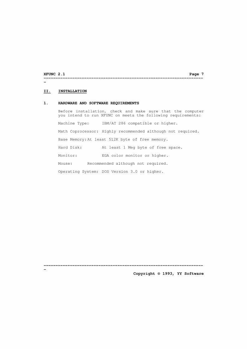
II. INSTALLATION 1. HARDWARE AND SOFTWARE REQUIREMENTS Before installation, check and make sure that the computer

you intend to run XFUNC on meets the following requirements: Machine Type: IBM/AT 286 compatible or higher. Math Coprocessor: Highly recommended although not required. Base Memory: At least 512K byte of free memory. Hard Disk: At least 1 Meg byte of free space. Monitor: EGA color monitor or higher. Mouse: Recommended although not required. Operating System: DOS Version 3.0 or higher.

XFUNC 2.1 --------------------------------------------------------------------


Page 8

2. INSTALLATION Installation is very simple. The best thing to do is to open

up a new directory called XFUNC and copy all the files into the directory. You must have the following files when you first received the program:

README.TXT Read this ASCII file before start. MANUAL.WP5 The User Manual in Word Perfect 5.1

format. XFUNC.BAT The batch file to start the XFUNC program. SHELL.EXE The XFUNC Shell, which lets the user

direct various operation toward different sub programs.

ANALYSIS.EXE This program calculates the transfer function

from a Circuit File. OPERATE.EXE This program does the interactive user

operation and plots graphs on the screen. REGISTER.EXE This program provides step by step instructions

to register XFUNC. XFUNC.HLP This is the indexed Help File to be used

by SHELL.EXE. XFUNC.CFG This is the Configuration File to be used

by OPERATE.EXE *.CIR A list of Circuit File examples. FASTDUMP.COM Utility program to dump any text screen or

graphic plot to the printer.

XFUNC 2.1 --------------------------------------------------------------------

--------------------------------------------------------------------


Page 9

III. PROGRAM OPERATION 1. INTEGRATED ENVIRONMENT Running the program in an Integrated Environment is what you

should do at the beginning. After you get familiar with the program, you might want to run the program under the DOS Command Line directly. To start XFUNC under the Integrated Environment, type

XFUNC [Enter] The XFUNC.BAT file calls the SHELL.EXE program to start the

program. The various menu selections are explained below. If you wish to plot graph or dump screen to a printer, before

you start XFUNC, type FASTDUMP and press [Enter]. Then follow the menu. The FASTDUMP utility allows you to dump the display to Epson, IBM Pro, HP Laserjet, or disk files, simply by pressing the [Print Screen] key. It is a memory resident program, but it consumes less than 8K byte of memory.

About - Information To display system information, etc. About - Program To display the XFUNC Version, Serial Number, etc. About - Register This selection is equivalent to typing REGISTER in the DOS

Command Line. It lets you execute the REGISTER.EXE program. The file REGISTER.TXT will be generated if you register.

File - File Name This selection lets you enter the File Name that you wish to

operate on. The File Name will not change throughout the

XFUNC 2.1 --------------------------------------------------------------------


Page 10

entire session until another File Name is entered. There are four types of files related to the same File Name:

Circuit File with a .CIR extension Output File with a .OUT extension Data File with a .DAT extension Modified Data File with a .MOD extension The Circuit File is where the user enter the circuit's

netlist description. The Output File, which is generated by the ANALYSIS.EXE program, gives the results of the circuit analysis. The Data File, which is also generated by the ANALYSIS.EXE program, allows other programs to read the results of the circuit analysis. The Modified Data File, which is generated by the SHELL.EXE program, stored the modified results of the analysis. The Data File and the Modified Data File have exactly the same file structure. You can rename a Data File to a Modified Data File or vice versa, but do not use an editor to modify these files. These files are explained in detail below.

File - Edit Circuit This selection opens up an ASCII editor which either creates

or retrieve the Circuit File. The Circuit File is the File Name selected above with a .CIR extension. Follow the instructions in Section 0 to enter the netlist description of the circuit.

File - View Output This selection opens up an ASCII viewer which let you browse

the Output File. The Output File is the File Name selected above with a .OUT extension.

File - Configure This selection lets you configure the OPERATE.EXE programs

for custom operations by editing the XFUNC.CFG file. The XFUNC.CFG settings affect only the OPERATE.EXE program. The ANALYSIS.EXE program is configured by the .OPTION statement

XFUNC 2.1 --------------------------------------------------------------------

--------------------------------------------------------------------


Page 11

in the Circuit File. See the explanations in 25 on how to select the various settings.

The settings of the XFUNC.CFG file is listed below. The

Defaults are settings when you first received the program. OPERATE.EXE will not run if an invalid option is entered. Therefore, keep a backup copy of the XFUNC.CFG file before changes are made. The parameters must appear in the following orders and no spaces are allowed at both sides of the equal sign.

i) Relative precision when two numbers are

compared: Default: PREC=1.0E+8 Range: 1.0E+3 to 1.0E+16 ii) Absolute precision when two numbers are

compared: Default: ZERO=1.0E-200 Range: 3.0E-308 to 1.0E-10 iii) Simplification methods: Default: SIMP=P Range: D, S, or P File - DOS Command This selection let you execute DOS commands directly. For

instance, if you want to use your favorite ASCII editor instead of the built-in editor to edit the Circuit File, you can enter your editor's name followed by the Circuit File name.

File - DOS Shell This selection takes you out into DOS directly. Type EXIT to

return from DOS. File - Quit

XFUNC 2.1 --------------------------------------------------------------------


Page 12

This selection terminates the SHELL.EXE program and returns

to DOS. Analysis - Go This selection is equivalent to typing ANALYSIS followed by

the File Name selected above in the DOS Command Line. It lets you execute the ANALYSIS.EXE program. The ANALYSIS.EXE program reads the Circuit File (.CIR extension) and generates the Output File (.OUT extension) and a Data File (.DAT extension).

Data - ... All selections under 'Data' calls the OPERATE.EXE program.

The OPERATE.EXE program cannot be run directly at the DOS Command Line.

Data - Load This selection lets you load a Data Object from the Data File

(.DAT extension) or the Modified Data File (.MOD extension). A Data Object might be the voltage across a Voltage Meter or the current through a Current Meter as specified as one of the outputs in the Circuit File. The Data File or Modified Data File can contain more than one Data Object. Choose only one Data Object from the given list. By loading the Data Object into memory, you can modify and plot the Data Object.

Data - Save This selection lets you save a Data Object into the Modified

Data File (with a .MOD extension) only. The Data Object can only be saved to the same name. You cannot save the Data Object into the Data File with a .DAT extension.

XFUNC 2.1 --------------------------------------------------------------------

--------------------------------------------------------------------


Page 13

Data - Window This selection switch your active window from the main menu

to the window showing the Data Object. It lets you view the Data Object by using the cursor keys.

Data - Modify This selection lets you modify mathematically the Data Object

loaded into memory. The following modifications can be done. Sign Change Change the sign (+/-) of the Data

Object. Inverse Inverse (1/X) the Data Object. Add by Add an Expression to the Data Object. Subtract by Subtract an Expression from the Data

Object. Multiply by Multiply an Expression to the Data

Object. Divide by Divide an Expression to the Data

Object. Substitute Substitute a symbol of the Data

Object with an Expression. Expression can be any valid mathematical expression that uses

+, -, *, /, or () as operators. You can use real numbers or symbols in the Expression.

XFUNC 2.1 --------------------------------------------------------------------


Page 14

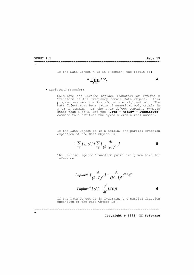
Data - f-t Transform This selection lets you transform the selected Data Object

from frequency domain to time domain. The following transformations can be performed.

Initial Value Calculate the initial value response to a step function

using the Initial Value Theorem. If the Data Object X is in S-domain, the result is:

If the Data Object X is in Z-domain, the result is:

Final Value Calculate the final value response to a step function

using the Final Value Theorem. If the Data Object X is in S-domain, the result is:

X(S)=S

Lim

1

X(Z)=Z

Lim

2

X(S)=0S

Lim

3

XFUNC 2.1 --------------------------------------------------------------------

--------------------------------------------------------------------


Page 15

If the Data Object X is in Z-domain, the result is:

Laplace,Z Transform Calculate the Inverse Laplace Transform or Inverse Z

Transform of the frequency domain Data Object. This program assumes the transforms are right-sided. The Data Object must be a ratio of numerical polynomials in S or Z domain. If the Data Object contains symbols other than S or Z, use the 'Data - Modify - Substitute' command to substitute the symbols with a real number.

If the Data Object is in S-domain, the partial fraction

expansion of the Data Object is:

The Inverse Laplace Transform pairs are given here for reference:

If the Data Object is in Z-domain, the partial fraction expansion of the Data Object is:

X(Z)=1Z

Lim

4

])P-(S

A[+]SB[=k

Mk

k

ii

ik 5

(t)][dtd=]S[Laplace i

ii1- 6

et1)!-(MA=]

P)-(SA[Laplace Pt1-M

M1-

XFUNC 2.1 --------------------------------------------------------------------


Page 16

The Inverse Z Transform pairs are given here for reference:

The result of Inverse Laplace Transform is expressed in

time t. The result of Inverse Z Transform is expressed in sample number n. Please refer to Reference by William H. Beyer for notations.

Since the Inverse Laplace and Inverse Z Transforms

require the use of partial fraction expansion, care must be taken to allow the program to recognize multiple roots. If some of the Ak values of Equation 5 and 7 have very large magnitude, it might be necessary to use a looser settings of PREC and ZERO in 'File - Configure' to allow the program to group multiple roots together.

If A = AR + j AI and P = PR + j PI are complex, the

partial fraction expansion must come with their complex conjugates A* and P*. Use the following equation as a guide.

])Ze-(1

A[+]ZB[=1-P M

k

k

i-i

i k k 7

i)-(n=]Z[Ztransfrom -i-1 8

(PI)]AI-(PI)[ARe2=eA+eA PRP*P * sincos 9

en!1)!-(M1)!-M+(nA=]

)Ze-(1A[Ztransform Pn

1-P M1-

XFUNC 2.1 --------------------------------------------------------------------

--------------------------------------------------------------------


Page 17

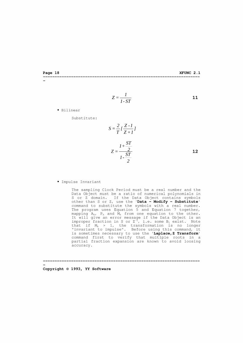
Data - S-Z Transform This selection lets you transform the selected Data Object

between S-domain and Z-domain. The following transformations can be performed. S and Z are the complex frequencies, and T is the sampling Clock Period that you can entered as an Expression.

Expression can be any valid mathematical expression that uses

+, -, *, /, or () as operators. You can use real numbers or symbols in the Expression.

Forward Derivative (Forward Euler Transform) Substitute:

Backward Derivative (Backward Euler Transform) Substitute:

ST+1=Z 10

T1-Z=S

TZ-1=S

-1

XFUNC 2.1 --------------------------------------------------------------------


Page 18

Bilinear Substitute:

Impulse Invariant The sampling Clock Period must be a real number and the

Data Object must be a ratio of numerical polynomials in S or Z domain. If the Data Object contains symbols other than S or Z, use the 'Data - Modify - Substitute' command to substitute the symbols with a real number. The program uses Equation 5 and Equation 7 together, mapping Ak, Pk and Mk from one equation to the other. It will give an error message if the Data Object is an improper fraction in S or Z-1, i.e. some Bi exist. Note that if Mk > 1, the transformation is no longer "invariant to impulse". Before using this command, it is sometimes necessary to use the 'Laplace,Z Transform' command first to verify that multiple roots in a partial fraction expansion are known to avoid loosing accuracy.

ST-11=Z 11

2

ST-12

ST+1=Z 12

]1+Z1-Z[

T2=S

XFUNC 2.1 --------------------------------------------------------------------

--------------------------------------------------------------------


Page 19

Data - Undo This selection lets you undo any changes to the Data Object. Plot - ... All selections under 'Plot' calls the OPERATE.EXE program.

The OPERATE.EXE program cannot be run directly at the DOS Command Line. In order to plot a Data Object onto the screen, the Data Object must be a ratio of numerical polynomials in S or Z domain. If the Data Object contains symbols other than S or Z, use the 'Data - Modify - Substitute' command to substitute the symbols with a real number before plotting.

Plot - Gain-Phase This selection plots or lists the gain and phase response of

the selected Data Object onto the screen. You can use automatic ranges or enter the ranges for frequency, magnitude, or phase. When automatic frequency range is selected, the program will select a frequency range that will cover all the poles and zeros of the Data Object. For S-domain, the magnitudes of the poles and zeros divided by 2π determine the frequencies. For Z-domain, the magnitudes of (one minus the poles and zeros) divided by 2π determine the frequencies.

Plot - Bode This selection plots or lists straight lines Bode Plot of the

selected Data Object onto the screen. The frequency range processing is exactly the same as the 'Plot - Gain-Phase' command. The Bode Plot represents frequency peaking with a vertical straight line. It shows the magnitude (Q Factor) at the frequency corner. Note that the Q Factor is not equivalent to the actual peaking, unless the Q Factor is high. Since there is no standard Bode Plot for Z-domain, a Z-domain Data Object is first converted to S-domain by substituting Z = 1 + S. This approximates ejω = 1 + jω for ω

XFUNC 2.1 --------------------------------------------------------------------


Page 20

much smaller than 1. Plot - Pole-Zero This selection plots or lists the pole and zero locations of

the selected Data Object onto the screen. A pole is represented by an 'X' and a zero by an 'O'. You have to be careful when counting poles and zeros. If two or more poles or zeros have the same location, they will overlap each other and cannot be distinguished.

Plot - Nyquist This selection plots a Nyquist Plot of the selected Data

Object onto the screen. The frequency range processing is exactly the same as the 'Plot - Gain-Phase' command. In most cases, there are no differences between Linear or Log frequency ranges. However, if there are significant discontinuities in the plot, switch between Linear and Log ranges to divide the frequency range in a different manner. If the discontinuities persist, use the 'Plot - Gain-Phase' command to narrow down the frequency range where the gain and phase change the most. Then manually enter the range for the Nyquist Plot.

Plot - Impulse This selection plots or lists the Impulse response of the

selected Data Object onto the screen. The program uses Equation 5 for S-domain or Equation 7 for Z-domain to calculate the time or sample response. For S-domain, the time response is a continuous function. For Z-domain, the program joins all sample data points with straight lines. If the Data Object is an improper fraction in S or Z-1, i.e. some Bi exist, the program will give an error message because

XFUNC 2.1 --------------------------------------------------------------------

--------------------------------------------------------------------


Page 21

it cannot plot delta functions. You can use automatic ranges or enter the ranges for time or sample, or magnitude. When automatic time or sample range is selected, the program will select a range that will cover the decaying time constant and the oscillation period of the Data Object. Before using this command, it is sometimes necessary to use the 'Laplace,Z Transform' command first to verify that multiple roots in a partial fraction expansion are known to avoid loosing accuracy.

Plot - Step This selection plots or lists the Step response of the

selected Data Object onto the screen. The transfer function to be plotted or listed is the Data Object multiplied by 1/S for S-domain or Z/(Z-1) for Z-domain. Plotting method is exactly the same as the 'Plot - Impulse' command.

F1=Help Pressing [F1] at any time opens up the Help Screen. You can

page through the information or use cross referencing to get to the help text.

XFUNC 2.1 --------------------------------------------------------------------


Page 22

2. DOS COMMAND LINE ENVIRONMENT The program REGISTER.EXE and ANALYSIS.EXE can be run under

DOS Command Line directly. The program OPERATE.EXE cannot be run under the DOS Command Line Environment. To run REGISTER.EXE, type the following command. The file REGISTER.TXT will be generated if you register.

REGISTER [Enter] To run ANALYSIS.EXE, type: ANALYSIS <File Name> [Enter] Where <File Name> is the Circuit File name (no .CIR extension

is needed). The ANALYSIS.EXE program will generate the Output File (with a .OUT extension) and the Data File (with a .DAT extension).

If you want to run several Circuit File at the same time, but

you don't want to wait for one Circuit File to finish before typing in the other, you can place the ANALYSIS <File Name> commands in a batch file (with a .BAT extension), say RUN.BAT:

ANALYSIS <File Name 1> ANALYSIS <File Name 2> .. .. ANALYSIS <File Name N> Then run all Circuit Files at once by typing: RUN [Enter].

XFUNC 2.1 --------------------------------------------------------------------

--------------------------------------------------------------------


Page 23

IV. WRITING A CIRCUIT FILE The Circuit File is an ASCII file (with a .CIR extension)

which describes the circuit to be analyzed. Each line of the Circuit File contains a circuit component description, the type of analysis to be made, the user option to control the analysis, or just a comment. These lines can be written in any order, as long as the list is ended with an End Line. You can use the 'File - Edit Circuit' command under the Integrated Environment to edit the Circuit File or you can use your favorite ASCII editor. Each type of lines are described in detail in the following sections.

XFUNC 2.1 --------------------------------------------------------------------


Page 24

1. COMMENT Syntax: ; <Any Comment> Example: ; This is a comment. Any characters to the right of the semicolon of the same line

is considered to be a Comment. Comment can be placed at the same line, but to the right of any circuit description lines.

2. CIRCUIT TITLE Syntax: .TITLE <Circuit title description> Example: .TITLE Low Noise Bandpass Filter. A circuit description title can be written at the .TITLE

line. This is useful for bookkeeping purposes. The .TITLE line can be written in upper or lower case letters.

XFUNC 2.1 --------------------------------------------------------------------

--------------------------------------------------------------------


Page 25

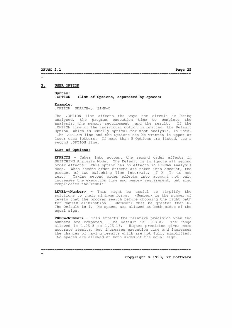
3. USER OPTION Syntax: .OPTION <List of Options, separated by spaces> Example: .OPTION SEARCH=5 SIMP=D The .OPTION line affects the ways the circuit is being

analyzed, the program execution time to complete the analysis, the memory requirement, and the result. If the .OPTION line or the individual Option is omitted, the Default Option, which is usually optimal for most analysis, is used. The .OPTION line and the Options can be written in upper or lower case letters. If more than 8 Options are listed, use a second .OPTION line.

List of Options: EFFECT2 - Takes into account the second order effects in

SWITCHING Analysis Mode. The Default is to ignore all second order effects. This option has no effects in LINEAR Analysis Mode. When second order effects are taken into account, the product of two switching Time Intervals, _T X _T, is not zero. Taking second order effects into account not only increases the execution time and memory requirement, but also complicates the result.

LEVEL=<Number> - This might be useful to simplify the

solutions to their minimum forms. <Number> is the number of levels that the program search before choosing the right path for matrix elimination. <Number> must be greater than 0. The Default is 1. No spaces are allowed at both sides of the equal sign.

PREC=<Number> - This affects the relative precision when two

numbers are compared. The Default is 1.0E+8. The range allowed is 1.0E+3 to 1.0E+16. Higher precision gives more accurate results, but increases execution time and increases the chances of having results which are not fully simplified. No spaces are allowed at both sides of the equal sign.

XFUNC 2.1 --------------------------------------------------------------------


Page 26

SEARCH=<Number> - This might be useful to simplify the

solutions to their minimum forms. <Number> is the number of searches per level that the program search before choosing the right path for matrix elimination. <Number> must be greater than 0. The Default is 1. No spaces are allowed at both sides of the equal sign.

SIMP=<Method> - This affects the simplification method to

used during the calculations. <Method> can be any one of the following:

D - Use detail simplification in all calculations. S - Use simple simplification in all calculations. P - Let the program decide when to use detail and when to use simple simplification. The Default is P. Using detail simplification usually

increases the execution time, but reduces the chances of having results which are not fully simplified. No spaces are allowed at both sides of the equal sign.

ZERO=<Number> - This affects the absolute precision when two

numbers are compared. The Default is 1.0E-200. The range allowed is 3.0E-308 to 1.0E-10. Lower zero setting gives more accurate results, but increases execution time and increases the chances of having results which are not fully simplified. No spaces are allowed at both sides of the equal sign.

XFUNC 2.1 --------------------------------------------------------------------

--------------------------------------------------------------------


Page 27

4. ANALYSIS MODE Syntax: <Analysis Mode> Example: .DC SWITCHING The Analysis Mode line tells the program what result is

needed from the analysis. One and only one Analysis Mode line must be included in the Circuit File. It can be written in upper or lower case letters.

List of Analysis Modes .AC LINEAR - The circuit is linear, and the result is given

in S-domain transfer function format. .DC LINEAR - The circuit is linear, and the result is given

in DC (S approaches 0). .AC SWITCHING - The circuit is switching, and the result is

given in Z-domain transfer function format. .DC SWITCHING - The circuit is switching, and the result is

given in DC (Z approaches 1).

XFUNC 2.1 --------------------------------------------------------------------


Page 28

5. INPUT SOURCE Syntax: <Source Type> <N+> <N-> <Expression> Example: VS 3 6 100.0 The Input Source is where the signal

originates. For AC Analysis Mode, one and only one Input Source is allowed. For DC Analysis Mode, at least one Input Source is allowed. <N+> and <N-> are the node numbers to which the Input Source is connected. Traditional SPICE node numbers are supported.

<Expression> defines the magnitude of

the Input Source. <Expression> can be any valid mathematical expression that uses +, -, *, /, or () as operators. You can use real numbers or symbols in the Expression. The symbols S and Z are reserved for the complex frequencies. Complex frequency S can only be used in LINEAR Analysis Mode. Complex frequency Z can only be used in SWITCHING Analysis Mode. If <Expression> is omitted, the Source Type (VS or IS) is used as a symbol for the magnitude of the Input Source. Symbols with more than 10 characters are truncated.

List of Source Type VS - Voltage Source with voltage output at node <N+> and

output return at node <N->. IS - Current Source which pulls current flowing into node

<N+>, through the Current Source, and push current out of

Figure 1 Input Sources

XFUNC 2.1 --------------------------------------------------------------------

--------------------------------------------------------------------


Page 29

node <N->.

XFUNC 2.1 --------------------------------------------------------------------


Page 30

6. OUTPUT METER Syntax: <Meter Type> <N+> <N-> Example: IM 0 11 The Output Meter is where the

measurement takes place. The output results are listed in the same order as the Output Meter statements are listed in the Circuit File. <N+> and <N-> are the node numbers to which the Output Meter is connected. Traditional SPICE node numbers are supported.

List of Meter Type VM - Voltage Meter with voltage input

at node <N+>, and input return at node <N->.

IM - Current Meter which monitors

current flowing into node <N+>, through the Current Meter, and out of node <N->.

Figure 2 Output Meters

XFUNC 2.1 --------------------------------------------------------------------

--------------------------------------------------------------------


Page 31

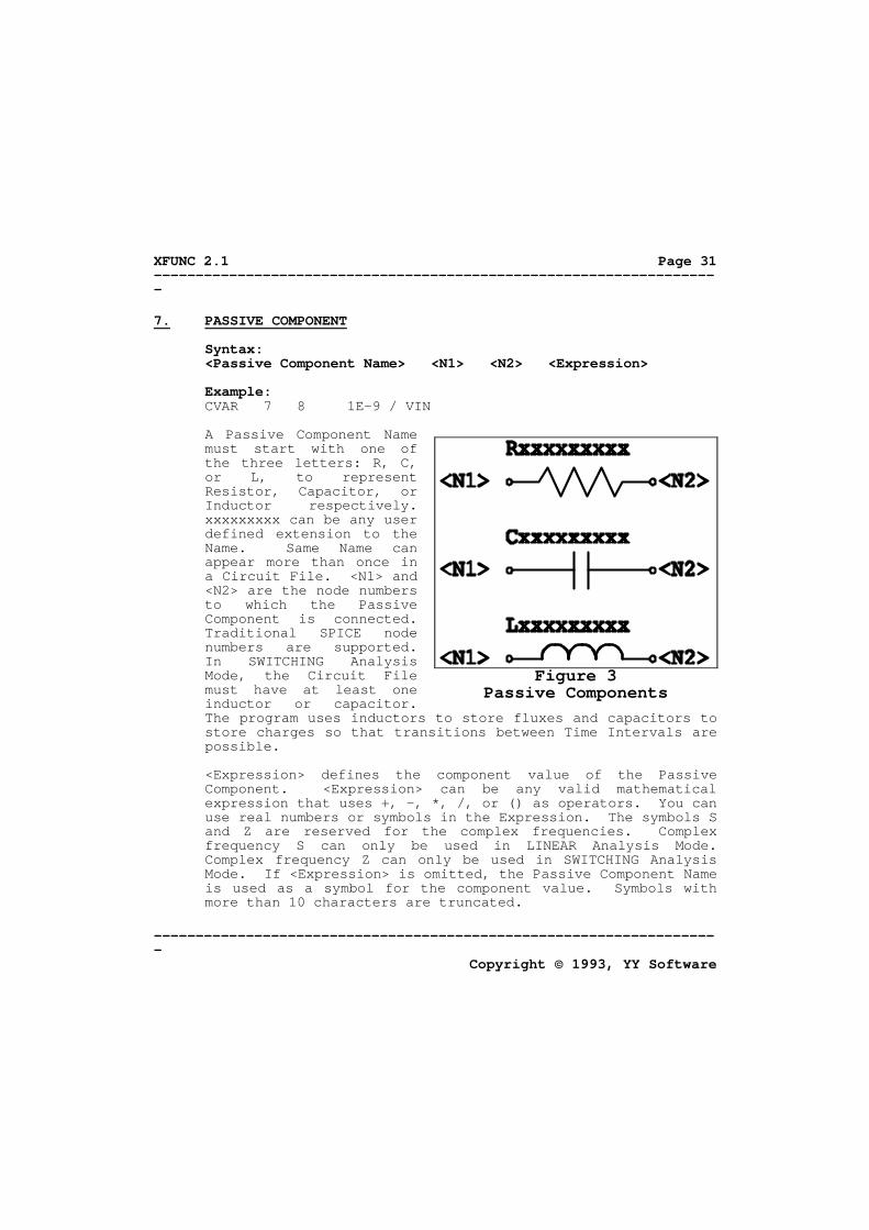
7. PASSIVE COMPONENT Syntax: <Passive Component Name> <N1> <N2> <Expression> Example: CVAR 7 8 1E-9 / VIN A Passive Component Name

must start with one of the three letters: R, C, or L, to represent Resistor, Capacitor, or Inductor respectively. xxxxxxxxx can be any user defined extension to the Name. Same Name can appear more than once in a Circuit File. <N1> and <N2> are the node numbers to which the Passive Component is connected. Traditional SPICE node numbers are supported. In SWITCHING Analysis Mode, the Circuit File must have at least one inductor or capacitor. The program uses inductors to store fluxes and capacitors to store charges so that transitions between Time Intervals are possible.

<Expression> defines the component value of the Passive

Component. <Expression> can be any valid mathematical expression that uses +, -, *, /, or () as operators. You can use real numbers or symbols in the Expression. The symbols S and Z are reserved for the complex frequencies. Complex frequency S can only be used in LINEAR Analysis Mode. Complex frequency Z can only be used in SWITCHING Analysis Mode. If <Expression> is omitted, the Passive Component Name is used as a symbol for the component value. Symbols with more than 10 characters are truncated.

Figure 3 Passive Components

XFUNC 2.1 --------------------------------------------------------------------


Page 32

List of Passive Components Rxxxxxxxxx - Resistor connected between node <N1> and <N2>. Cxxxxxxxxx - Capacitor connected between node <N1> and <N2>. Lxxxxxxxxx - Inductor connected between node <N1> and <N2>.

XFUNC 2.1 --------------------------------------------------------------------

--------------------------------------------------------------------


Page 33

8. LINEAR DEPENDENT SOURCE Syntax: <Source Name> <NO+> <NO-> <NI+> <NI-> <Expression> Example: HIE 11 12 3 0 100 / (S + 100) A Dependent Source Name

must starts with one of the three letters: E, F, G or H, to represent the type of Dependent Sources. xxxxxxxxx can be any user defined extension to the Name. Same Name can appear more than once in a Circuit File. <NO+>, <NO->, <NI+>, and <NI-> are the node numbers to which the Dependent Source is connected. Traditional SPICE node numbers are supported.

<Expression> defines the

gain factor of the Dependent Source. <Expression> can be any valid mathematical expression that uses +, -, *, /, or () as operators. You can use real numbers or symbols in the Expression. The symbols S and Z are reserved for the complex frequencies. Complex frequency S can only be

Figure 5 Linear Dependent Sources

XFUNC 2.1 --------------------------------------------------------------------


Page 34

used in LINEAR Analysis Mode. Complex frequency Z can only be used in SWITCHING Analysis Mode. If <Expression> is omitted, the Dependent Source Name is used as a symbol for gain factor. Symbols with more than 10 characters are truncated.

List of Dependent Source Names Exxxxxxxxx - Voltage Control Voltage Source with voltage

output at node <NO+> and output return at node <NO->, and voltage input at node <NI+>, and input return at node <NI->.

Fxxxxxxxxx - Current Control Current Source which pulls

current flowing into node <NO+>, through the Source, and push current out of node <NO->, and control current flowing into node <NI+>, through the Control, and out of node <NI->.

Gxxxxxxxxx - Current Control Voltage Source which pulls

current flowing into node <NO+>, through the Source, and push current out of node <NO->, and voltage input at node <NI+>, and input return at node <NI->.

Hxxxxxxxxx - Voltage Control Current Source with voltage

output at node <NO+> and output return at node <NO->, and control current flowing into node <NI+>, through the Control, and out of node <NI->.

XFUNC 2.1 --------------------------------------------------------------------

--------------------------------------------------------------------


Page 35

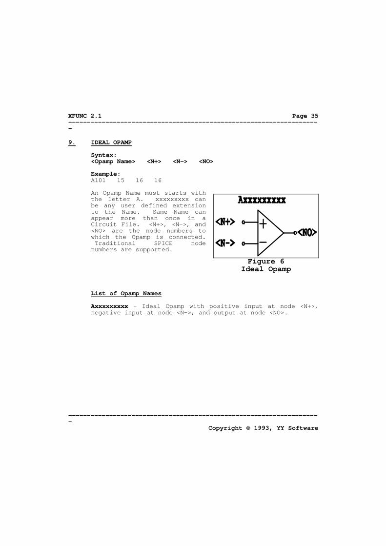
9. IDEAL OPAMP Syntax: <Opamp Name> <N+> <N-> <NO> Example: A101 15 16 16 An Opamp Name must starts with

the letter A. xxxxxxxxx can be any user defined extension to the Name. Same Name can appear more than once in a Circuit File. <N+>, <N->, and <NO> are the node numbers to which the Opamp is connected. Traditional SPICE node numbers are supported.

List of Opamp Names Axxxxxxxxx - Ideal Opamp with positive input at node <N+>,

negative input at node <N->, and output at node <NO>.

Figure 6 Ideal Opamp

XFUNC 2.1 --------------------------------------------------------------------


Page 36

10. SWITCH Syntax: <Switch Name> <N1> <N2> Example: S1 6 0 A valid Switch Name is

S1, S2,.., to S9. <N1> and <N2> are the node numbers to which the Switch is connected. Traditional SPICE node numbers are supported. The Switch Name tells the program at what Time Interval the Switch is closed. Switch S1 is closed only during Time Interval 1, Switch S2 is closed only during Time Interval 2, etc. A corresponding Time Interval Declaration line for each Time Interval must be included in the Circuit File. No Switch is allowed under LINEAR Analysis Mode.

Whether the Switch breaks or makes before or after the

transition between Time Intervals depends on the circuit itself. The switch is designed such that capacitor charges and inductor fluxes are passed from one Time Interval to the next without overlapping and without loss of energy.

List of Switch Name S1 to S9 - Switch connected between node <N1> and <N2>.

Figure 7 Switch

XFUNC 2.1 --------------------------------------------------------------------

--------------------------------------------------------------------


Page 37

11. TIME INTERVAL DECLARATION Syntax: <Time Interval> <Expression> Example: T2 (1 - d) / Fo A valid Time Interval is T1, T2,.., to T9. At the first Time

Interval T1, all the switches with Switch Name S1 are closed, at the second Time Interval T2, all the switches with Switch Name S2 are closed, etc. Time Interval must start from T1 and goes up. Time Interval cannot be declared more than once. The circuit's Output Meter (VM or IM) samples the output at the end of the last Time Interval just before the start of the next Clock Period. At least one Timing Interval Declaration is needed under SWITCHING Analysis Mode. No Timing Interval Declaration is allowed under LINEAR Analysis Mode.

Since state-space averaging analysis technique is used, Time

Intervals are assumed to be much smaller than the circuit's time constants.

<Expression> defines the duration in time of the Time

Interval. Therefore, the sum of the durations of all the Time Intervals declared in the Circuit File is the Clock Period. <Expression> can be any valid mathematical expression that uses +, -, *, /, or () as operators. You can use real numbers or symbols in the Expression. The symbols S and Z are reserved for the complex frequencies. Complex frequency S can only be used in LINEAR Analysis Mode. Complex frequency Z can only be used in SWITCHING Analysis Mode. If <Expression> is omitted, the Time Interval Name (T1, etc) is used as a symbol for the duration in time. Symbols with more than 10 characters are truncated.

List of Time Intervals T1 to T9 - Time Interval.

XFUNC 2.1 --------------------------------------------------------------------


Page 38

12. END LINE Syntax: .END Example: .END The .END line must be included to complete the Circuit File.

Any statements after the .END line is disregarded by the program. The .END line can be written in upper or lower case letters.

XFUNC 2.1 --------------------------------------------------------------------

--------------------------------------------------------------------


App A-1

APPENDIX A: APPLICATION NOTES

APPENDIX A

APPLICATION NOTES

XFUNC 2.1 --------------------------------------------------------------------


App A-2

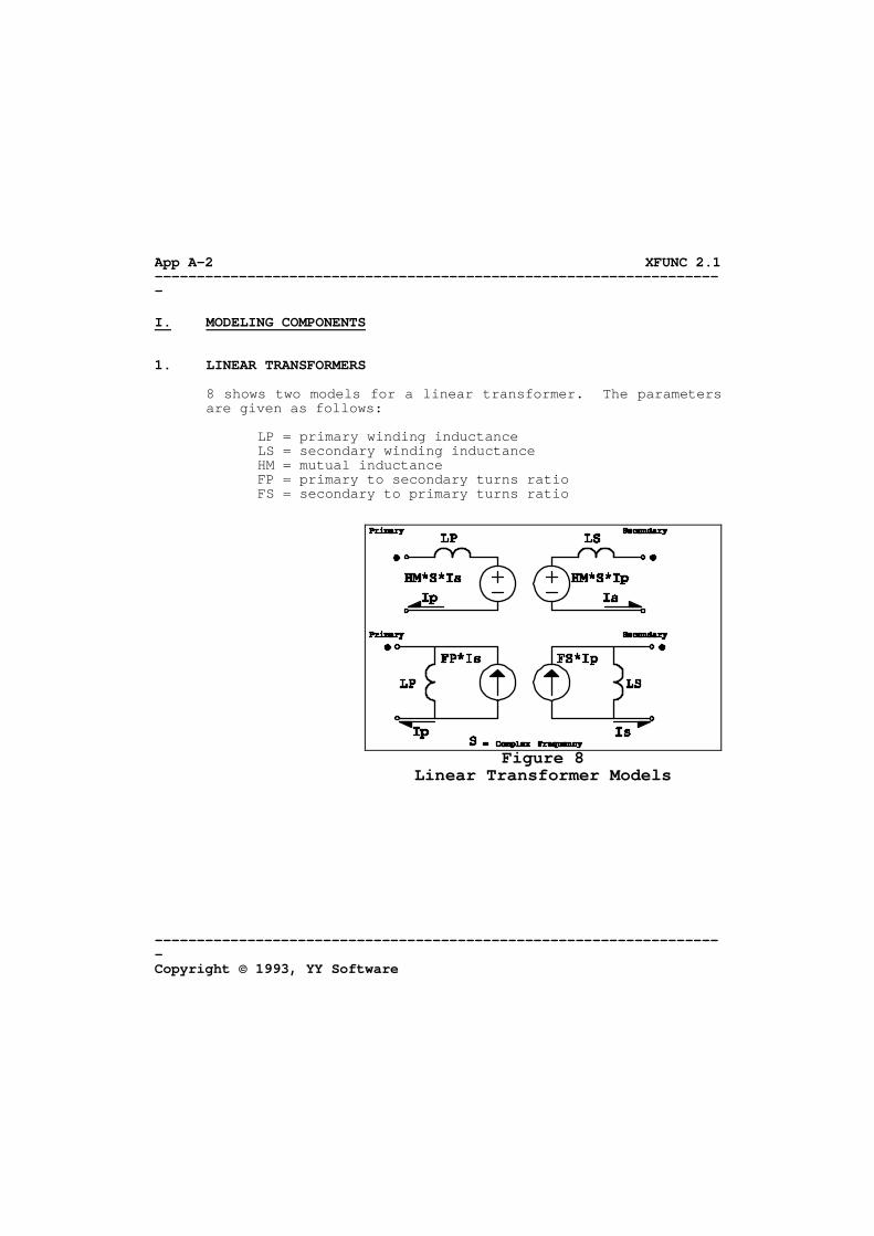
I. MODELING COMPONENTS 1. LINEAR TRANSFORMERS 8 shows two models for a linear transformer. The parameters

are given as follows: LP = primary winding inductance LS = secondary winding inductance HM = mutual inductance FP = primary to secondary turns ratio FS = secondary to primary turns ratio

Figure 8 Linear Transformer Models

XFUNC 2.1 --------------------------------------------------------------------

--------------------------------------------------------------------


App A-3

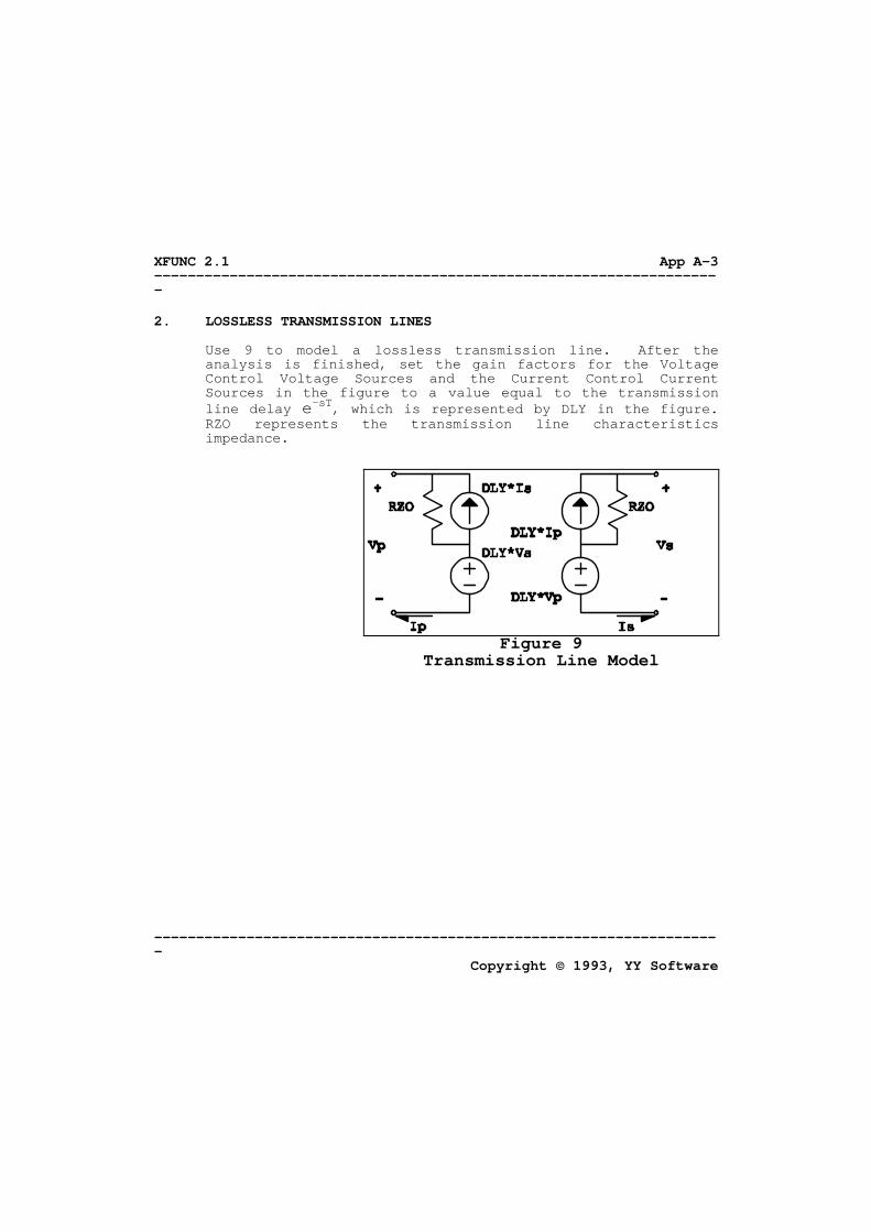
2. LOSSLESS TRANSMISSION LINES Use 9 to model a lossless transmission line. After the

analysis is finished, set the gain factors for the Voltage Control Voltage Sources and the Current Control Current Sources in the figure to a value equal to the transmission line delay e-sT, which is represented by DLY in the figure. RZO represents the transmission line characteristics impedance.

Figure 9 Transmission Line Model

XFUNC 2.1 --------------------------------------------------------------------


App A-4

II. FILES TRANSFER DIAGRAM

10 shows how files are transferred when XFUNC is operating under the Integrated Environment. The order that steps are taken might not need to follow the numbers labeled next to the arrow. Nevertheless, these numbers let us go through the complete process as an example.

Step 1: The user reads the README.TXT and MANUAL.WP5 files

and understand the program operation.

Figure 10 Files Transfer Diagram

XFUNC 2.1 --------------------------------------------------------------------

--------------------------------------------------------------------


App A-5

Step 2: The user executes the program via XFUNC.BAT. Step 3: XFUNC.BAT calls SHELL.EXE to start the program. Step 4: SHELL.EXE reads the XFUNC.HLP file to make Help

information available to the user. Step 5: SHELL.EXE edits the Circuit File (<File Name>.CIR)

via the built-in editor. Step 6: SHELL.EXE passes the File Name to ANALYSIS.EXE and

ask it to perform a circuit analysis on the Circuit File (<File Name>.CIR).

Step 7: ANALYSIS.EXE reads the Circuit File (<File

Name>.CIR). Step 8: When ANALYSIS.EXE finished the task successfully, it

generates the Output File (<File Name>.OUT) and the Data File (<File Name>.DAT).

Step 9: SHELL.EXE views the Output File (<File Name>.OUT) via

the built-in viewer. Step 10: SHELL.EXE loads one of the Data Object in the Data

File (<File Name>.DAT) to be modified as needed. Step 11: XFUNC.CFG might need some modifications by SHELL.EXE

before OPERATE.EXE is executed. Step 12: SHELL.EXE places the Data Object data, the requested

modifications, etc. into the Temporary Files. Step 13: SHELL.EXE passes the requested modification commands

to OPERATE.EXE and ask it to perform an operation on the Temporary Files.

Step 14: OPERATE.EXE reads the XFUNC.CFG file to configure

its internal registers. Step 15: OPERATE.EXE reads the Temporary Files, performs the

requested operation, and modifies the Temporary Files.

XFUNC 2.1 --------------------------------------------------------------------


App A-6

Step 16: SHELL.EXE reads back the Temporary Files which store

the operation results. Step 17: OPERATE.EXE saves the results into the Modified Data

File (<File Name>.MOD). Step 18: SHELL.EXE calls the REGISTER.EXE program. Step 19: REGISTER.EXE generates the REGISTER.TXT file.

XFUNC 2.1 --------------------------------------------------------------------

--------------------------------------------------------------------


App A-7

III. LINEAR CIRCUIT ANALYSIS TECHNIQUES 1. INPUT AND OUTPUT IMPEDANCES For small signal linear models, the input impedance is

defined as the input voltage divided by the input current, and the output impedance the open-circuit output voltage divided by the short-circuit output current. If we disable the independent sources of the circuit by replacing all independent Voltage Sources by a short-circuit and all independent Current Sources by an open-circuit, then the output impedances can be found using the same method as for the input impedances. The following shows the Circuit File example to calculate impedances:

IS 0 1 1.0 VM 1 0 ; Connect your circuit between nodes 1 and 0 to calculate the ; impedance. Remember Ohm's Law: V=IR. V = R if I = 1. 2. LINEAR CIRCUIT EQUATIONS (XFUNC'S OPERATION) To review, the impedance expressed in S-domain for a resistor

R is just R, for a capacitor C is 1 / (C * S), and for an inductor L is L * S, where S is the Laplace complex frequency.

Kirchhoff's Current Law states that the total current flowing

into a node should sum up to zero. To make the Law useful for us, the program groups the nodes at both side of a (dependent or independent) Voltage Source to form a supernode. The output of an opamp is grouped with ground. Therefore, the Law can be applied to supernodes instead of just nodes. Thus, Kirchhoff's Current Law equations can be written. The total number of unknown node voltages and the total number of equations must be equal or else, the circuit has 'Conflicting error'. But grouping two nodes together means that we have one less equation to solve. The other equation we need is the voltage gain equations of a dependent Voltage Source and the opamp.

XFUNC 2.1 --------------------------------------------------------------------


App A-8

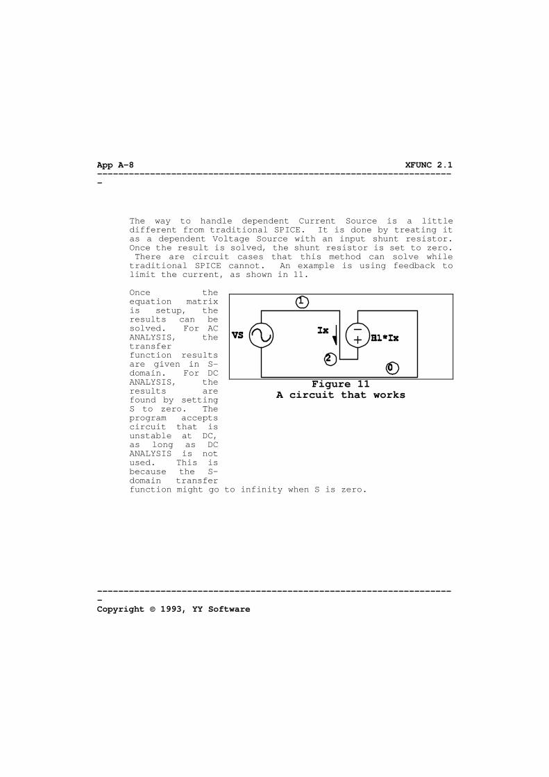
The way to handle dependent Current Source is a little

different from traditional SPICE. It is done by treating it as a dependent Voltage Source with an input shunt resistor. Once the result is solved, the shunt resistor is set to zero. There are circuit cases that this method can solve while traditional SPICE cannot. An example is using feedback to limit the current, as shown in 11.

Once the

equation matrix is setup, the results can be solved. For AC ANALYSIS, the transfer function results are given in S-domain. For DC ANALYSIS, the results are found by setting S to zero. The program accepts circuit that is unstable at DC, as long as DC ANALYSIS is not used. This is because the S-domain transfer function might go to infinity when S is zero.

Figure 11 A circuit that works

XFUNC 2.1 --------------------------------------------------------------------

--------------------------------------------------------------------


App A-9

IV. SWITCHING CIRCUIT ANALYSIS TECHNIQUES 1. STATE SPACE AVERAGING (XFUNC'S OPERATION) 12 shows an

example of a circuit's state variable changing over time. A state variable is either the voltage across a capacitor or the current through an inductor. The state variable is similar to the Z-1 delay element in digital filters. Inputs and outputs to the switching circuit are being sampled at the end of the Clock Period just before the switches change state. Since this is a sample data system, any glitches in between sampling at the input signals or output signals will have no effects to the overall transfer function. The outputs are determined by the capacitor voltages, inductor currents, and the input signals only at the time when samples are taken.

Figure 12 State Switching Example

XFUNC 2.1 --------------------------------------------------------------------


App A-10

The diagram in 13 shows how the program represents a

switching circuit with three Z-1 elements representing three capacitor voltages or inductor currents states. In general, any switching circuit can be represented in similar fashion. Each Amplifier in the figure has a gain factor. The Amplifiers' gain factors form the Transition Matrix. The Transition Matrix is calculated in two steps. First, the input X and the present states SPRESENT affect the next states SNEXT, as given by the following equation:

Figure 13 Input/Output relationship

XFUNC 2.1 --------------------------------------------------------------------

--------------------------------------------------------------------


App A-11

Once the matrices [A] and [B] are solved by superposition, the present states SPRESENT can be solved as a function of Z. Then, the input X and the present states SPRESENT affect the output Y, as given by the following equation:

Using superposition, the matrices [C] and [D] can be solved. The output Y is found by direct substitution of SPRESENT. One might be interested to convert the result back to S-domain. This program provides several ways to transform from Z-domain to S-domain: Forward or Backward Derivatives (Euler Transform), Bilinear, or Impulse Invariant Transforms. Refer to 17 for details. Forward or Backward Derivatives are recommended to reduce the complexity of the transformed result, although it might be necessary to use the other methods sometimes.

When converting from Z-domain to S-domain, it is sometimes

necessary to multiply the Z transfer function result by Z or 1/Z before applying the transformation equation so that the S-domain result is in its simplest form. This is because 1/Z is a delay element in Z-domain. The delay has a gain of one and the phase is linear. At frequencies much smaller than the Clock frequency, the delay can be neglected.

2. STATE CHANGE CALCULATION (XFUNC'S OPERATION) In each Time Interval, we can construct a circuit using the

information given on the positions of the switches. The state variables are the initial voltages across the capacitors and the initial currents through the inductors. This can be think of as having all capacitors charged and inductors fluxed and then build the circuit in zero seconds. The state variables we are interested in are the capacitor

ZS=S=S[A]+[B]X PRESENTNEXTPRESENT 13

Y=S[C]+[D]X PRESENT 14

XFUNC 2.1 --------------------------------------------------------------------


App A-12

voltages and inductor currents at the end of the Time Interval right before the switches change positions for the next Time Interval.

How does the input signal X causes the change in state

variables? We can setup the circuit and monitor the state variables as our output with an input step function (X = 1/S). Then, by using Linear Analysis technique, the state variable output Y can be found as a function of S since Y = <circuit's transfer function in S-domain> * X. By applying Initial Value Theorem, the initial value Yo of the state variable can be found:

The change of the state variable during the Time Interval can be found by first finding the time differential dY/dt of the state variable:

Then applying the Initial Value Theorem to the time differential gives the initial time differential:

The state variable Y1 at the end of the small Time Interval T1 is therefore approximated by:

How does a state variable causes the change of itself or other state variables? The same steps as above are taken, but instead of an input step function, the initial value

[YS]=YS

o Lim

15

Y-YS=dtdY

o 16

17

18

XFUNC 2.1 --------------------------------------------------------------------

--------------------------------------------------------------------


App A-13

generators are used. The initial value generator of a charged capacitor is a parallel Current Source with magnitude equal to the initial capacitor voltage times the capacitance. The initial value generator of a fluxed inductor is a parallel Current Source with magnitude equal to the initial inductor current divided by S.

Since we are dealing with linear circuits, the Principle of

Superposition applies. The effects of each state variable and the effects of the input can be calculated separately. Thus an overall transition matrix for one Time Interval can be found. It maps the input and the state variables before the Time Interval to the state variables after the Time Interval.

The transition matrices for all Time Intervals are multiplied

to form the transition matrix for one Clock Period. Second order effects are ignored if:

where dY/dto1 * T1 is the time differential change during Time Interval T1 and dY/dto2 * T2 is the time differential change during Time Interval T2.

19

XFUNC 2.1 --------------------------------------------------------------------


App A-14

V. ERRORS AND PROBLEMS 1. ERROR CODES A. SHELL.EXE Errors There are two types of errors that can occur. One is fatal

error which will terminate the program immediately with a beeping sound. The other error type is non-fatal and it will only notify the user with a pop-up window about the error and that the program is unable to perform the task that the user asks for. There are too many non-fatal error messages to list here, but basically they are classified into six types:

i) Disk Allocation Error: Check to make sure that the hard disk drive is not

write protected and there is enough disk space for operations and file transfers.

ii) Memory Allocation Error: Try to take out as many memory resident programs from

your computer as possible. iii) Missing File Error: Make sure that all the necessary files as listed in

Section 0 are under the same directory as the SHELL.EXE program.

iv) Operation Error: If this happens, check and redo what needs to be done

and everything will be fine. v) Program Limitation Error: This means that the program is not designed to be

capable of handling the task you ask it to perform. Try to simplify the task.

XFUNC 2.1 --------------------------------------------------------------------

--------------------------------------------------------------------


App A-15

vi) Unable to Execute Error: The sub-program cannot be executed either because the

program file (.EXE extension) is missing or there is not enough memory available to run the sub-program.

XFUNC 2.1 --------------------------------------------------------------------


App A-16

B. ANALYSIS.EXE Errors Whenever an error is encountered, the program will be

terminated with a beeping sound. An error message with a blinking 'ERROR' will be displayed on the screen. The Output File will contain the nature and explanations of the error that happened.

Abnormal termination: This occurs if there are hardware or software

incompatibilities. Check the setup and installation procedures and hardware and software requirements described in this Manual. If all fails, contact the software manufacturer.

Cannot find roots: This error could be caused by 'Conflicting error' described

in this section. Use the same steps described in 'Conflicting error' to clear the problem. Another possible cause is that the circuit entered is too big and complicated to be analyzed. Try to break up a big circuit into smaller blocks and analyzes each block individually. Also, try not to use the SEARCH or LEVEL options, if they are set, and try not to use the SIMP=D option so that the polynomial root finder routine is not called as much. If all failed, use the SIMP=S option and use a looser PREC and ZERO settings.

Cannot write Data File: Data File cannot be created or written to. This happens if

the output disk space is full or the output disk space is write protected.

Cannot write Output File: Output File cannot be created or written to. This happens if

the output disk space is full or the output disk space is write protected.

Conflicting error: For linear circuits, make sure that the circuit does not

contain any floating nodes or shorted loops. For switching circuit, make sure that in all Time Intervals, the circuit with the specified switch positions does not contain any

XFUNC 2.1 --------------------------------------------------------------------

--------------------------------------------------------------------


App A-17

floating nodes or shorted loops. Floating-point error: This error could be caused by 'Conflicting error' or 'Cannot

find roots' described in this section. Use the same steps described in 'Conflicting error' or 'Cannot find roots' to clear the problem. Another possible cause is that the circuit entered is too big and complicated to be analyzed. Try to break up a big circuit into smaller blocks and analyze each block individually. Another possible cause is that the numerical value for the components and parameters are either too big (say > 1E+100 or too small (say < 1E-100). Also, try to change the mathematical options in the .OPTION line.

Memory check failed: When the program terminates, it frees all the memory it used.

This error occurs if the memory available when the program begins is not the same as the memory available when the program terminates. Try to take out as many memory resident programs as possible.

Missing Circuit File: Circuit File is missing or cannot be read. Circuit File must

have a .CIR extension, and it must reside in the same directory as where the .EXE program resides, unless the directory is specified in the File Name.

Out of memory: If you are running the program under the Integrated

Environment, try to run it under the DOS Command Line instead. Also, the circuit entered might be too big to be analyzed. Try to break the circuit into smaller blocks, and analyzes each block individually. Try to reduce the number of different symbols by substituting the symbols with real numbers. Take out as many memory resident programs from your computer as possible. Try not to use the SEARCH or LEVEL options, if they are set, and try to use the SIMP=D option to minimize the memory needed.

Power overflow: The circuit entered might be too big to be analyzed. Try to

break the circuit into smaller blocks, and analyzes each

XFUNC 2.1 --------------------------------------------------------------------


App A-18

block individually. Try not to use the SEARCH or LEVEL options, if they are set, and try to use the SIMP=D option to minimize the symbolic variables' power.

Program error: This error occurs if there are some bugs in the program which

are trapped by the program itself. Contact the software manufacturer if this happens.

Symbolic math error: This error could be caused by 'Conflicting error' described

in this section. Use the same steps described in 'Conflicting error' to clear the problem.

Syntax error: The Circuit File contains syntax error. The Output File

should contain the explanations and location of the syntax error.

Undocumented error: This should never happen. Contact the software manufacturer

if it does. User break: You have pressed the [Esc] or [Ctrl] C key to stop the

program.

XFUNC 2.1 --------------------------------------------------------------------

--------------------------------------------------------------------


App A-19

C. OPERATE.EXE Errors Whenever an error is encountered, the program will be

terminated. An error message with a blinking 'ERROR' will be displayed on the screen.

Abnormal termination. This occurs if there are hardware or software

incompatibilities. Check the setup and installation procedures and hardware and software requirements described in this Manual. If all fails, contact the software manufacturer.

Cannot find roots. This error indicates that the polynomial root finder routine

is unable to find a root. The Data Object must be a fairly high order polynomial (> 20) of some symbol. Try adjust the configuration in the XFUNC.CFG file from SIMP=D to SIMP=P or to SIMP=S to avoid using the root finder routine. If this fail, try adjust the PREC and ZERO settings in the XFUNC.CFG file to a looser degree, i.e. use smaller PREC value and higher ZERO value, to make it easier to converge. Finally, try to minimize the size of the Data Object. If this error occurs during 'Plot - Gain-Phase' or 'Plot - Nyquist' command, try to avoid using automatic frequency ranges.

Cannot read from file. This may happen if there is not enough disk space to store

the Temporary Files, the disk is write protected, or the disk has error.

Cannot write to file. This may happen if there is not enough disk space to store


Data error in file. This may happen if there is not enough disk space to store


Expression error.

XFUNC 2.1 --------------------------------------------------------------------


App A-20

The Expression you entered at a prompt to a menu selection contains syntax error. Re-enter the Expression.

Floating-point error. This happens if you selected an invalid operation, such as

divide by zero, etc, or if you enter an invalid plot range when trying to plot a Data Object. A plot range is invalid if the number is too large or too small. Using automatic range might clear the problem. For Gain-Phase, Bode, or Nyquist plots, this error might happen if the plot range contains a pole at infinity. This error might also be related to the 'Cannot find roots' error. Use the same steps described in 'Cannot find roots' to clear the problem. Also try to adjust the settings in the XFUNC.CFG file.

Graphic error. This means that probably this program is incompatible with

the graphic hardware installed in your computer. Check the setup and installation procedures and hardware and software requirements described in this Manual.

Improper fraction. The menu selection does not allow the Data Object to be an

improper fraction in S or Z-1. There is nothing wrong with the Data Object itself.

Invalid configuration. The XFUNC.CFG file contains invalid configuration

information. Adjust the settings in the XFUNC.CFG file back to valid ranges. If you do not remember how to adjust the XFUNC.CFG file, replace the current copy of the file with the original copy. This will reset the configuration to the Defaults.

Memory check failed. When the program terminates, it frees all the memory it used.

This error occurs if the memory available when the program begins is not the same as the memory available when the program terminates. Try to take out as many memory resident programs as possible.

XFUNC 2.1 --------------------------------------------------------------------

--------------------------------------------------------------------


App A-21

Not numerical coeff. The menu selection requires that the Data Object to be a

ratio of numerical polynomial in S or Z only. No symbols are allowed in the Data Object except either S or Z. There is nothing wrong with the Data Object itself. Use the 'Data - Modify - Substitute' command in the menu selection to substitute all other symbols with a real number.

Out of memory. Take out as many memory resident programs from your computer

as possible. Try adjust the configuration in the XFUNC.CFG file from SIMP=S to SIMP=P or to SIMP=D to minimize the memory needed. Try to reduce the size of the Data Object by substituting the symbols with real numbers.

Power overflow. The power of any symbol in the Data Object is too high. Try

adjust the configuration in the XFUNC.CFG file from SIMP=S to SIMP=P or to SIMP=D to reduce the power to a minimum. Try to reduce the size of the Data Object.

Program error. This error occurs if there are some bugs in the program which

are trapped by the program itself. Contact the software manufacturer if this happens.

Symbolic math error. This may occur under the same conditions as the 'Floating-

point error'. Use the same steps described in 'Floating-point error' to clear the problem.

Undefined operation. This may occur under the same conditions as the 'Out of

memory' error. Use the same steps described in 'Out of memory' to clear the problem. The computer might have run out of environment space also.

XFUNC 2.1 --------------------------------------------------------------------


App A-22

Undocumented error. This should never happen. Contact the software manufacturer

if it does. User break. You have pressed the [Ctrl] C or [Ctrl] [Break] key to stop

the program.

XFUNC 2.1 --------------------------------------------------------------------

--------------------------------------------------------------------


App A-23

2. AVOIDING PROBLEMS AND ERRORS The things to remember about entering the circuit is to avoid

any floating nodes or shorted loops. For switching circuits, avoid floating nodes or shorted loops for all defined switch positions at all Time Intervals.

Floating nodes are nodes that can assume any voltages,

independent of the circuit's component and parameter values. The example in 14 works fine in the real world, but it causes problems when analyzed by XFUNC.

E1 and E2 might

simulate transformers or isolation amplifiers. Although the output voltage at node 4 can be found, the voltages at node 2 and node 3 relative to ground (node 0) are unknown. Since we know that any voltage at node 3 gives the same result, node 3 should be connected to ground.

Shorted loops are loops that can assume any current. A real

world example of shorted loops are ground loops in a poorly designed instrument. Shorted loops usually do not cause errors when analyzed by XFUNC, but they should be avoided to prevent incorrect results. 15 shows an example of a shorted loop.

Figure 14 Floating Nodes

XFUNC 2.1 --------------------------------------------------------------------


App A-24

The circuit

shows that node 2 must have a zero voltage relative to ground, so a current equal to VS / RS flows from the input Voltage Source. But where does the current go? There is no way to determine how the current is divided into Ix and Iy, although XFUNC will divide the current equally between them under this situation.

Another thing to remember is for switching circuits, the

output is always sampled at the end of the last Time Interval. Consider the switch capacitor integrator circuit in 15.

Figure 15 Shorted Loops

XFUNC 2.1 --------------------------------------------------------------------

--------------------------------------------------------------------


App A-25

The voltage at

node 2 is calculated to be zero, since the Capacitor C1 is shorted to ground at the end of the last Time Interval (at T2 when S2 is closed). However, if we exchange switches S1 and S2 in the circuit, the voltage at node 2 is calculated to be VS. With S1 and S2 exchanged, the Capacitor C1 is shorted to the input Voltage Source at the end of the last Time Interval. Moreover, with the circuit as shown, the output voltage at node 4 is calculated to be one clock cycle ahead of the same output if S1 and S2 were exchanged. This is because with the circuit as shown, the voltage at VS is being passed to C1 at the first Time Interval T1, and the voltage at C1 is being passed to C2 at the next Time Interval T2. But with S1 and S2 exchanged, the voltage at C1, which was already charged at the last Clock Period, is being passed to C2 at the first Time Interval T1, and at the next Time Interval T2, C1 acquires the voltage VS, to be used for the next Clock Period. Thus voltage information is always one Clock Period behind. This explains why sometimes it is necessary to multiply the Z-domain transfer function by Z or 1/Z to adjust the Clock Period delay appropriately.

Figure 16 Switch Capacitor Integrator

XFUNC 2.1 --------------------------------------------------------------------


App A-26

Consider another interesting situation as in 17 and 17. These two circuits are stray-insensitive switch capacitor integrators. When analyzed by XFUNC, the one in 17 will result in a transfer function of 1 / (1 - Z), while the one in 17 will result in a transfer function of 1 / (Z - 1). However, if you connect the output of 17 to the input of 17 and analyze them together, the result will be -Z / (Z*Z - 2*Z + 1) which is not equal to multiplying 1 / (1 - Z) and 1 / (Z - 1) together. The result is one Clock Period ahead of what is expected. Why does this happen is left to you to find out. This is not caused by a bug in the program. Hint: Remember that the output is always sampled at the end of the Clock Period.

Figure 17

XFUNC 2.1 --------------------------------------------------------------------

--------------------------------------------------------------------


App A-27

Figure 18

XFUNC 2.1 --------------------------------------------------------------------


App A-28

3. EXISTING PROBLEMS AND BUGS MEMORY ACCESS VIOLATION The ANALYSIS.EXE and OPERATE.EXE programs use recursive

routines to access recursive data structures. It was found that with some EMS software installed, the programs lock up when the recursive routines ran out of working space. Ideally, the program should flag 'Out of memory' error.

POLYNOMIAL ROOT FINDER CONVERGENCE PROBLEM The polynomial root finder routine uses the Laguerre's Method

for root finding and polishing. It was found that in some cases when the polynomial order became too high (say > 20), the method did not converge, but oscillated up and down. Finding accurate multiple roots are also difficult, but this is true in general for any polynomial root finder routines. We welcome any donation of a good polynomial root finder routine in the C language.

NOT FAST ENOUGH All the symbolic math routines are written in the C language

only. Most of them have not been optimized for speed. It is believed that writing the code in Assembly Language or streamlining and eliminating some redundant task will improve the speed. However, no matter how slow this program is, it is still faster than doing the mathematics by paper and pencil. You might also notice that the XFUNC EDITOR is very slow. It is designed to handle very small files only.

XFUNC 2.1 --------------------------------------------------------------------

--------------------------------------------------------------------


App A-29

VI. OPTIMIZING THE RESULTS 1. ANALYSIS.EXE CALCULATIONS Although this program is basically for Electronics, one can

never get away from understanding the basic principles of Mathematics. The various Options in the .OPTION line of a Circuit File allow the user to modify the mathematical functions of the ANALYSIS.EXE program to optimize between the execution time, memory requirement, precision of the results, and factorization and simplification of the results. If you do not run into problems of this sort, you can run the program using its Default mathematical Options. Otherwise, you might need to understand how various Options play.

If your input Circuit File contains a lot of symbols, and you

found that the results are not fully simplified, then the SIMP=D option is recommended. If SIMP=D is not specified, all the symbols will get added and multiplied when solving the matrices. The symbolic variables are being looked at and analyzed in detail only at places where the program thinks that it is absolutely necessary. However, by the time when the variables are being analyzed in detail, the variables might have already accumulated a large number of terms which makes it impossible or time consuming to simplify. On the other hand, if SIMP=D is specified, the variables are analyzed and simplified in detail in every mathematical step. Obviously, the execution time will be increased, but the number of terms in the variables will get limited to its minimum possible. So, in most cases, the results are fully simplified.

If SIMP=D does not work, you might want to try the SEARCH and

LEVEL options. When a system of linear equations is to be solved, the equations are placed into a matrix. Choosing the row and column (the pivot) of the matrix to be eliminated significantly affects whether the end result is fully simplified or not. The SEARCH and LEVEL options allow the program to make trials when picking the pivot so that the end result has the minimum number of terms. LEVEL specifies how deep the program should look. SEARCH specifies how many

XFUNC 2.1 --------------------------------------------------------------------


App A-30

trials to make per LEVEL. For example, to solve a matrix of size 10 X 10 with LEVEL=3 and SEARCH=5, the program picks five different pivots to end up with five 9 X 9 matrices. For each 9 X 9 matrix, the program picks five different pivots to end up with a total of twenty five 8 X 8 matrices, until 125 7 X 7 matrices are generated. The 7 X 7 matrix with the minimum number of terms are chosen as the end result. Then from the 7 X 7 matrix, 125 4 X 4 matrices are generated, etc, until the end result is found. This is why the SEARCH and LEVEL options increases the execution time significantly. The SEARCH and LEVEL options can be used together with the SIMP=D option to optimize the results.

If you are only interested in getting a transfer function

with numerical coefficients so that you can plot the data, it is always recommended to use real number in the Expression for a component value instead of using symbol and then substitute the symbol with a real number after the analysis is done. A Circuit File with a lower number of symbols always make the program run faster and increase the chance of getting fully simplified results.

Then, what is the difference between putting a symbolic

Expression for a component value and do the analysis, versus putting a single symbol for a component value and substitute the symbol with the symbolic Expression when the analysis is done? That depends on how many similar symbols in the Circuit File, how many similar symbols in the final results, and how the symbols cancel each other. You are encourage to try either way and find out which methods serve the best.

For Circuit File which contains mostly numbers, the effects

of SIMP, SEARCH, and LEVEL are basically the same. With numbers, one has to worry about precision of the results. When a seemingly 6-pole transfer function becomes 8-pole, it is possible that two zeros and two poles are not close enough to be cancelled. When the matrix is solved, the machine's inaccuracy grows very fast, especially when there is a small difference of two large numbers. Therefore, if SIMP=D is not specified, by the time when the end result is being simplified in detail, the errors in the coefficients of the polynomials will be so large that the poles and zeros are too

XFUNC 2.1 --------------------------------------------------------------------

--------------------------------------------------------------------


App A-31

far apart to be cancelled. This happens even at 53 bits of double precision arithmetics if the order of the polynomial is high. Using SIMP=D, roots are cancelled before they have a chance to accumulate error. The SEARCH and LEVEL options avoid generating higher order polynomials so as to avoid pole-zero cancellation as much as possible. If all these fails, the PREC and ZERO options are useful for number comparison. PREC affects the relative precision when two numbers are compared to be equal or not. ZERO affects the absolute precision. Therefore by reducing the PREC and increasing the ZERO options, a pole and a zero, which are considered as too far apart with the program's Default settings can be considered as equal.

For Circuit File with a lot of symbols, in most cases, it is

recommended to use a loose PREC and ZERO settings because the program does not need high precision to perform symbolic calculations.

XFUNC 2.1 --------------------------------------------------------------------


App A-32

2. OPERATE.EXE CALCULATIONS The XFUNC.CFG file contains various parameters to configure

the calculations of the OPERATE.EXE program to optimize between the execution time, memory requirement, precision of the results, and factorization and simplification of the results. If you do not run into problems of this sort, you can run the program using the Default settings, which are in the XFUNC.CFG file when you first received the program. Otherwise, you might need to understand how various parameters play.

Unlike the ANALYSIS.EXE program, memory requirement and

execution time are seldom issues for the OPERATE.EXE program. It is always recommended to use the SIMP=P or SIMP=D setting over the SIMP=S setting, unless the execution time is too long to be patient, or a 'Cannot find roots' error occurred. There are very little differences between the SIMP=P and SIMP=D settings, both of which make the program analyze and simplify the symbolic variables at every mathematical step. Therefore, in most cases, the results are fully simplified.

The PREC and ZERO settings are useful for number comparison.

PREC affects the relative precision when two numbers are compared to be equal or not. ZERO affects the absolute precision.

Under the 'Data' menu selection, for example, a Data Object

3/(X+1) is to be subtracted by 2/(X+1). The display rounds off any real numbers to about 6 significant digits. Therefore, the X+1 displayed on the screen could actually be X+1.0000001 or X+0.9999999. Thus it is possible for the result of the subtraction to have a quadratic function of X in the denominator. This can be avoided by using a smaller PREC setting. While the PREC setting is used to null out small differences of large numbers, the ZERO setting is used to null out larger differences of smaller numbers. For instance, two numbers 2.01E-50 and 2.00E-50 are to be subtracted. Just by using a smaller setting of PREC will not force the result to zero (unless it is smaller than the allowed range) because both numbers are very small. By setting ZERO to 1E-50, any number whose absolute value is

XFUNC 2.1 --------------------------------------------------------------------

--------------------------------------------------------------------


App A-33

less than 1E-50 will be forced to zero. The PREC and ZERO settings play an important role in any menu

selections that involve partial fraction expansion, such as the 'Laplace,Z Transform', 'Impulse Invariant', 'Plot - Impulse' and 'Plot - Step'. The partial fraction expansion requires that multiple roots be known. If the Data Object contains multiple roots, but the PREC and ZERO settings are too tight to recognize that, the Ak values of Equation 5 and Equation 7 will end up to be a large number. This is not an error, but your end result might loose significant accuracy.

XFUNC 2.1 --------------------------------------------------------------------


App A-34

VII. FURTHER IMPROVEMENTS The suggestions in this section are not implemented in this

version. The discussions that followed are purely imaginative and has no technical justifications. This section only provides possible improvements to the program.

ADD IMPORT AND EXPORT FEATURES The program should allow the Data Object to be imported from

or exported to other software packages such as SPICE, MATHCAD, NAG, etc. Also it should allow the Data Object to be read into the Circuit File.

ADD DIFFERENTIATION AS A MENU SELECTION Using differentiation, sensitivity analysis of a Data Object

is easy matter. More important, it is possible to calculate the frequency response of pulse-width modulation (PWM) and pulse-frequency modulation (PFM) circuits. After a Z-domain transfer function is calculated, one can transform it to S-domain with clock frequency F0, or duty ratio D as one of its symbol. Then by differentiating the Data Object with respect to F0 or D, one can calculate the AC response of the frequency to voltage gain of the PFM circuit, or the duty ratio to voltage gain of the PWM circuit. This, of course, assumes that F0 is much higher than the frequencies of interest of the AC response. To add the menu selection is easy. To prove that this is the correct way to calculate AC response of PFM or PWM circuits needs some research.

SOMETHING FOR SWITCHING CONVERTERS AND PHASE-LOCK LOOP This version cannot analyzes switching power converters under

discontinuous mode of operation. The reason is that the Time Interval is dependent on the circuit's voltages and currents. This implies finding roots for a symbolic polynomial, which is impossible to do, unless the polynomial is a quadratic. This problem can be circumvented if we add an additional component: a Voltage or Current control Time Interval Declaration. That will also help the accurate simulation of

XFUNC 2.1 --------------------------------------------------------------------

--------------------------------------------------------------------


App A-35

phase-lock loop opened-loop AC response. We have not figure out how easy and how useful it is to add the component.

LOW ENTROPY EXPRESSION One of the most important features of XFUNC is its ability to

express results in symbolic expression formats. However, the expression usually have too many terms to be useful to the user. One method is to use low entropy expression. Instead of using a simple ratio of polynomial expression, the program should allow the user to select different ways to express the same symbolic expression, that is, able to place parenthesis in the results to simplify the expression. This can be accomplished using different binary-tree type link-list structure to express the Data Object. By introducing a new operator (||), the parallel combination - i. e. product over sum: A * B / (A + B), the result should be further simplified.

ELIMINATE REDUNDANT CALCULATIONS It is believe that a lot of the execution time is wasted on

doing redundant task, such as simplifying a variable that has already been simplified. A way to avoid this is to attach to each symbolic variable a history log of where the variable has been through. Another good idea is to use the standard Maple symbolic library by the University of Waterloo, Canada, although fitting the library into the XFUNC environment might take some effort.

OTHER SIMPLE ADDITIONS * The OPERATE.EXE program should let the user generate an

ASCII list of data points in a file during a 'Plot - List' option.

* The OPERATE.EXE program should be able to use FFT as

another method to convert from frequency to time domain. * The OPERATE.EXE program should allow the user to substitute

mathematical functions such as EXP (X), SIN (X), etc, into

XFUNC 2.1 --------------------------------------------------------------------


App A-36

symbols for plotting purpose.

XFUNC 2.1 --------------------------------------------------------------------


Printed in U.S.A.

END OF DOCUMENT

Documents

XFUNC - Inicial — UFRGS XFUNC.pdf · The purpose of the program XFUNC is to compute the frequency domain transfer function of a circuit in symbolic format, given a circuit description