XI. INTRODUCTION TO QUANTUM MECHANICS

C. Cohen-Tannoudji et al., Quantum Mechanics I, Wiley.

Outline:

Electromagnetic waves and photons

Material particles and matter waves

Quantum description of a particle: wave packets

Particle in a time-independent scalar potential

Electromagnetic waves and photons

Light quanta and the Planck-Einstein relations

Planck (1900): the hypothesis of the quantization of energy: For an electro-magnetic wave of frequency ν, the only possible energies are integral multiples ofthe energy quantum hν (or ~ω), where h is a new fundamental constant.

Einstein (1905): the particle theory of light: Light consists of a beam of photons,each possessing an energy hν.

(Experimental verification: Compton (1924)).

The interaction of an electromagnetic wave with matter occurs by means of ele-mentary indivisible processes, in which the radiation appears to be composed ofparticles, the photons.

Planck-Einstein relations:

E = hν = ~ω

~p = ~~k

~ =h

2π

where h ≈ 6.62×10−34J.s is the Planck constant, ω = 2πν, and∣∣∣∣~k∣∣∣∣ = 2π/λ is the wave

vector.

Wave - particle duality

Young’s slit experiment

If both slits, F1 and F2 are open, the intensity of the light emitted from a monochro-matic light source S on the screen I(x) shows interference fringes, i.e.

I(x) , I1(x) + I2(x)

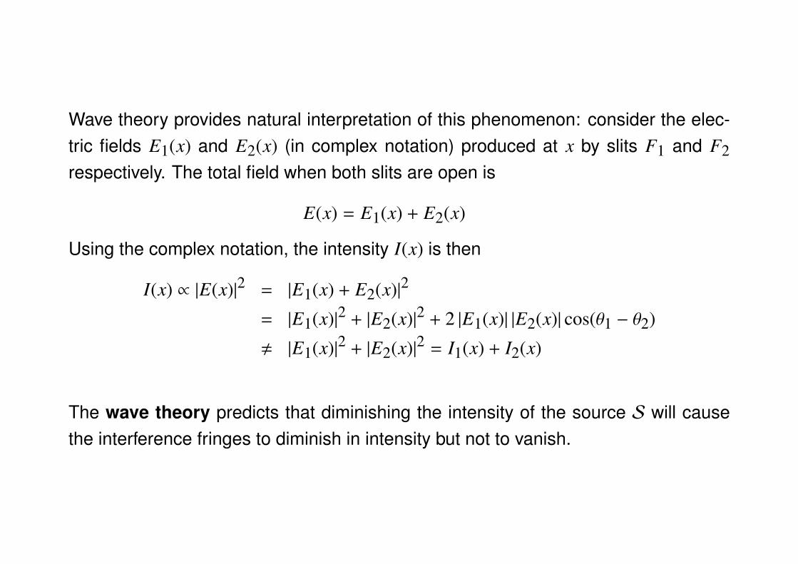
Wave theory provides natural interpretation of this phenomenon: consider the elec-tric fields E1(x) and E2(x) (in complex notation) produced at x by slits F1 and F2respectively. The total field when both slits are open is

E(x) = E1(x) + E2(x)

Using the complex notation, the intensity I(x) is then

I(x) ∝ |E(x)|2 = |E1(x) + E2(x)|2

= |E1(x)|2 + |E2(x)|2 + 2 |E1(x)| |E2(x)| cos(θ1 − θ2)

, |E1(x)|2 + |E2(x)|2 = I1(x) + I2(x)

The wave theory predicts that diminishing the intensity of the source S will causethe interference fringes to diminish in intensity but not to vanish.

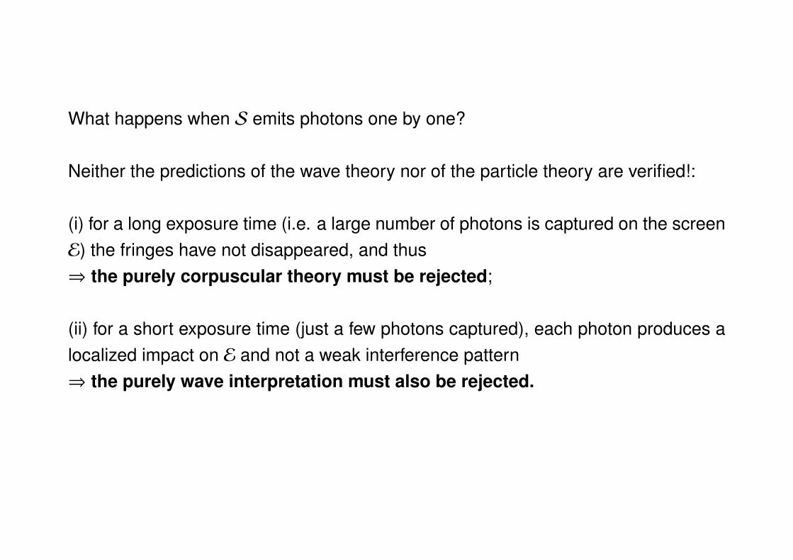
What happens when S emits photons one by one?

Neither the predictions of the wave theory nor of the particle theory are verified!:

(i) for a long exposure time (i.e. a large number of photons is captured on the screenE) the fringes have not disappeared, and thus⇒ the purely corpuscular theory must be rejected;

(ii) for a short exposure time (just a few photons captured), each photon produces alocalized impact on E and not a weak interference pattern⇒ the purely wave interpretation must also be rejected.

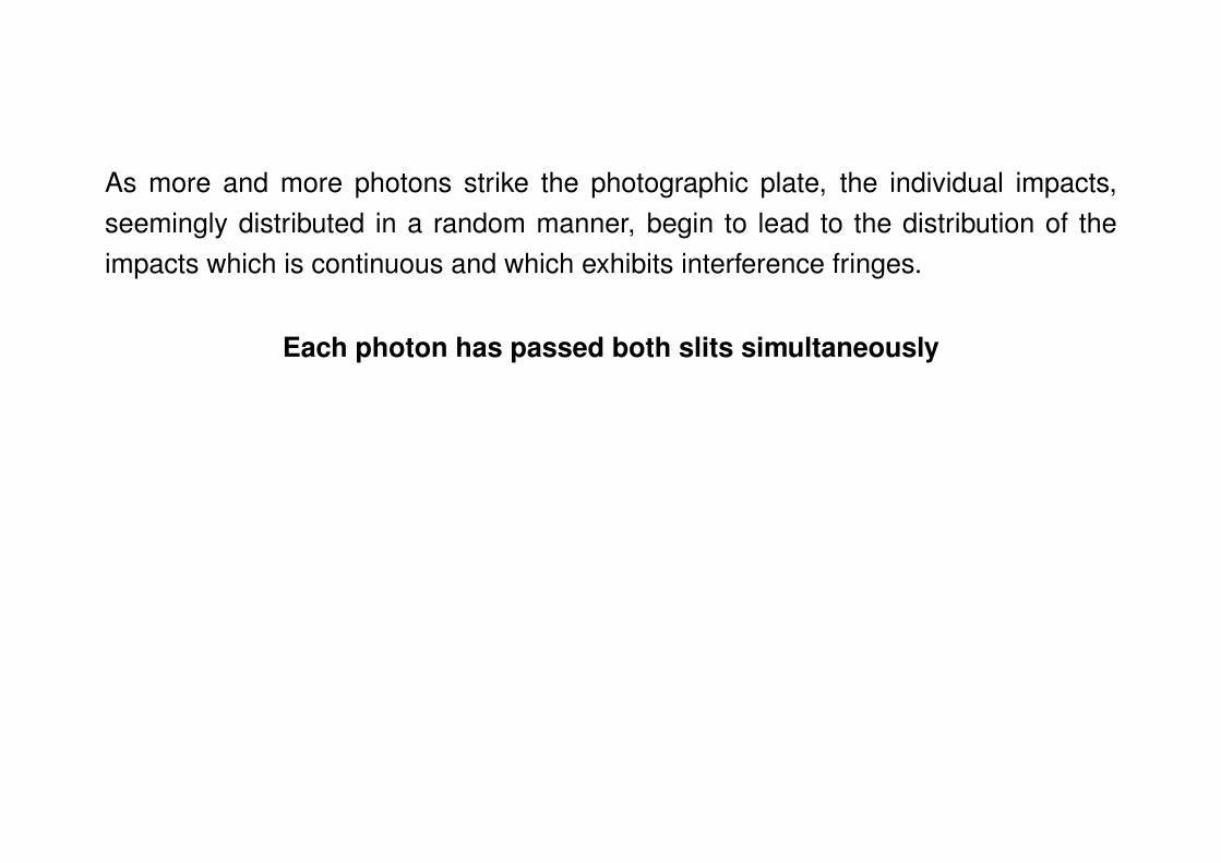
As more and more photons strike the photographic plate, the individual impacts,seemingly distributed in a random manner, begin to lead to the distribution of theimpacts which is continuous and which exhibits interference fringes.

Each photon has passed both slits simultaneously

Quantum unification of the two aspects of lightWe need to fundamentally reconsider the concepts of classical physics to unite twoaspects, wave or particle, of light.

For example, if we put a photodetector behind F2 only a half of the photons passthrough F2 and the other half through F1, giving just a single slit signal on E:

⇒ when one performs a measurement on a microscopic system, one disturbs itin a fundamental fashion;⇒ it is impossible to observe the interference pattern and to know at the same timethrough which slit each photon has passed.

Therefore, we are led to question the concept of a particle’s trajectory which is fun-damental one of classical physics.

Moreover, as the photons arrive one by one, their impacts on the screen build up theinterference pattern

⇒ for a particular photon, we are not certain in advance where it will strike the screen;

⇒ as these photons are emitted under the same conditions, it implies that the clas-sical idea that the initial conditions completely determine the subsequent motion of aparticle is invalid in quantum mechanics.

The concept of wave-particle duality:

(i) the particle and wave aspects of light are inseparable:Light behaves simultaneously like a wave and like a flux of particles, the wave en-abling us to calculate the probability of the manifestation of a particle;

(ii) predictions about the behaviour of a photon can only be probabilistic;

(iii) the information about a photon at time t is given by the wave E(~r, t) whichis a solution of Maxwell’s equation, and which characterizes the state of thephotons at time t.E(~r, t) is interpreted as the probability amplitude of a photon appearing, at time t, atthe point ~r = (x, y, z). The corresponding probability is proportional to

∣∣∣E(~r, t)∣∣∣2.

Comments:(i) If E1 and E2 are two solutions of Maxwell’s equation (which are linear and homo-geneous) then

E = λ1E1 + λ2E2

where λ1, λ2 are constants, is also a solution.

This implies superposition principle and its consequences, e.g. interference, diffrac-tions etc.

(ii) The theory merely allows to calculate the probability of the occurrence of a givenevent. Experimental verifications are to be founded on the repetition of a large num-ber of identical experiments (a large number of identically prepared particles, pho-tons).

(iii) Optical analogy: we can regard the quantum state of a material particle charac-terized by

a wavefunction ψ(~r, t)

in a similar way as we regard ”the photon state” E(~r, t).

The fact that ψ(~r, t) is complex is essential in quantum mechanics.

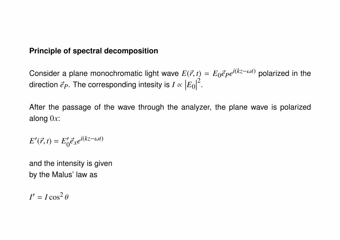
Principle of spectral decomposition

Consider a plane monochromatic light wave E(~r, t) = E0~ePei(kz−ωt) polarized in thedirection ~eP. The corresponding intesity is I ∝

∣∣∣E0∣∣∣2.

After the passage of the wave through the analyzer, the plane wave is polarizedalong 0x:

E′(~r, t) = E′0~exei(kz−ωt)

and the intensity is givenby the Malus’ law as

I′ = I cos2 θ

What will happen on the quantum level, when I is weak and photons reach the ana-lyzer one by one?

(1) photon either crosses the analyzer or it is entirely absorbed by it;

(2) we cannot in general predict with certainty whether a given photon will pass orwill be absorbed;

(3) for a large number N of equally prepared photons, the result will correspondto the classical law, i.e. N cos2 θ photons will pass.

These observations have several important implications:(i) the measurement device can give only certain privileged results, called

eigen results.

There is quantization of the results of the measurement (in contrast to the classicalcase).(ii) to each of the eigen results corresponds

an eigenstate.

For example, ~eP = ~ex (in the case that the photon pass the analyzer with certainty),or ~eP = ~ey (if it is absorbed with certainty).

If the particle is, before the measurement, in one of the eigenstates, the result ofthis measurement is certain: it can only be the associated eigen result.

(iii) when the state before the measurement is arbitrary, only the probabilities of ob-taining the different eigen results can be predicted.

To find these one decomposes the state of the particles into a linear combinationof the various eigenstates – this is the spectral decomposition:

~eP = ~ex cos θ + ~ey sin θ

where cos θ and sin θ are the probability amplitudes. The corresponding probabili-ties, which are cos2 θ and sin2 θ, statisfy

cos2 θ + sin2 θ = 1.

(iv) The measurement disturbs the microscopic system in a fundamental fashion:after passing through the analyzer, the light is completely polarized along ~ex.

Material particles and matter wavesThe de Broglie relations

Atomic emission and absorption spectra are composed of narrow lines, that is, agiven atom emits and absorbs only photons with well defined frequencies (energies)

⇒ the energy of the atom is quantized(Bohr-Sommerfeld (empirical) quantization of electron orbits)

hνi j =∣∣∣Ei − E j

∣∣∣where l.h.s. corresponds to the energy of the photon, and r.h.s. to that of the atom.

de Broglie hypothesis:

material particles, just like photons, can have a wavelike aspect.

This permits derivation of the Bohr-Sommerfeld quantization rules:

the various permitted energy levels appear as analogues of the normal modes ofa vibrating string

Davisson and Germer (1927) confirmed the de Broglie hypothesis by showing thatinterference patterns could be obtained with material particles like electrons.

Consider a material particle of energy E and momentum ~p and associate with it awave of angular frequency ω = 2πν and wave vector ~k. Then the relations

E = hν = ~ω

~p = ~~k

imply the de Broglie relation for the wavelength associated with a material particle

λ =2π∣∣∣∣~k∣∣∣∣ =

h∣∣∣~p∣∣∣

Examples:

(i) a dust particle: diameter d = 1 µm, m = 10−15 kg, speed v = 10−3 ms−1:

λ ≈6.6 × 10−34

10−15 × 10−3= 6.6 × 10−16 m = 6.6 × 10−6 Å

(ii) a thermal neutron: mn ≈ 1.67 × 10−27 kg, the speed is calculated as:

12

mnv2 =p2

2mn≈

32

kT

where k = 1.38 × 10−23 JK−1 is the Boltzmann constant. De Broglie wavelength isthen

λ =hp

=h

√3mnkT

which for T = 300 K gives λ ≈ 1.4 Å, which is about the interatomic distance in acrystal.

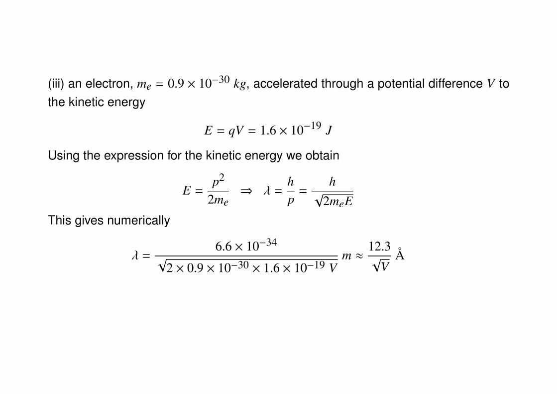
(iii) an electron, me = 0.9 × 10−30 kg, accelerated through a potential difference V tothe kinetic energy

E = qV = 1.6 × 10−19 J

Using the expression for the kinetic energy we obtain

E =p2

2me⇒ λ =

hp

=h

√2meE

This gives numerically

λ =6.6 × 10−34

√2 × 0.9 × 10−30 × 1.6 × 10−19 V

m ≈12.3√

VÅ

Wavefunctions. Schrodinger equation

We now apply the ideas introduced for the case of the photon to all material particles:

(i) The quantum state of a particle is characterized by a wavefunction ψ(~r, t), whichcontains all the information that is possible to obtain about the particle;

(ii) ψ(~r, t) is interpreted as a probability amplitude of the particle’s presence at thepoint ~r at time t;

The probability dP(~r, t) of the particle being at time t in a volume element d3r = dx dy dzsituated at the point ~r is interpreted as the corresponding probability density

dP(~r, t) = C∣∣∣ψ(~r, t)

∣∣∣2 d3r

where C is a normalization constant.

(iii) The principle of spectral decomposition applies to the measurement of an arbi-trary physical quantity:

- the result found must belong to a set of eigen results {a};

- with each eigenvalue a is associated an eigenstate, i.e. an eigenfunction ψa(~r)such that if ψ(~r, t0) = ψa(~r), the measurement (at t0) will always yield a;

- for any ψ(~r, t), the probability of finding the eigenvalue a for a measurement attime t0 is found by decomposing ψ(~r, t0) in terms of the functions ψa(~r):

ψ(~r, t0) =∑

acaψa(~r)

Then

Pa =|ca|

2∑a |ca|

2

where the denominator ensures that the total probability∑

aPa = 1 (normalization).

- if the measurement indeed yields a, the wavefunction immediately after the mea-surement is:

ψ′(~r, t0) = ψa(~r)

This is known as wavefunction collapse.

(iv) The evolution of the wavefunction ψ(~r, t) of a particle of mass m subjected to apotential V(~r, t) is governed by the Schrodinger equation

i~∂

∂tψ(~r, t) = −

~2

2m∆ψ(~r, t) + V(~r, t)ψ(~r, t)

where ∆ = ∂2/∂x2 + ∂2/∂y2 + ∂2/∂z2 is the Laplace operator.

The fact that the Schrodinger equation is linear and homogeneous in ψ implies that

there exists a superposition principle which, combined with the interpretation ofψ as a probability amplitude, is the source of wavelike effects, that is, it leads to

wave-particle duality.

Comments:

(i) For a system composed of only one particle, the total probability of finding theparticle anywhere in space, at time t, equals to 1:∫

dP(~r, t) = 1

Since dP(~r, t) = C∣∣∣ψ(~r, t)

∣∣∣2 d3r, this implies that the wavefunction must be square-integrable: ∫ ∣∣∣ψ(~r, t)

∣∣∣2 d3r < ∞

The normalization constant C is then given by the relation

1C

=

∫ ∣∣∣ψ(~r, t)∣∣∣2 d3r

We say that a wavefunction is normalized if C = 1:∫ ∣∣∣ψ(~r, t)∣∣∣2 d3r = 1

(ii) ψ(~r, t) is interpreted as a probability amplitude of the particle’s presence at thepoint given by the spatial coordinates ~r at time t: the wavefunction ψ(~r, t) character-izes a quantum state in the coordinate representation.

(iii) In general, it may be useful to represent a quantum state by other than coor-dinate representation.

For example, ψ(~p) is interpreted as a probability amplitude that the particle has themomentum ~p (at some fixed t); and the wavefunction ψ(~p) characterizes a quantumstate in the momentum representation.

(iv) The relation between the wavefunctions in the coordinate and momentum repre-sentations is given by the Fourier transform.

In one-dimensional systems this is given as

ψ(p) =1√

2π~

∫ +∞

−∞

dxe−ipx/~ψ(x)

The inverse formula is then

ψ(x) =1√

2π~

∫ +∞

−∞

dpeipx/~ψ(p)

Remark:while ψ(x) is an eigenstate of the coordinate operator, ψ(~p) is an eigenstate of themomentum operator.

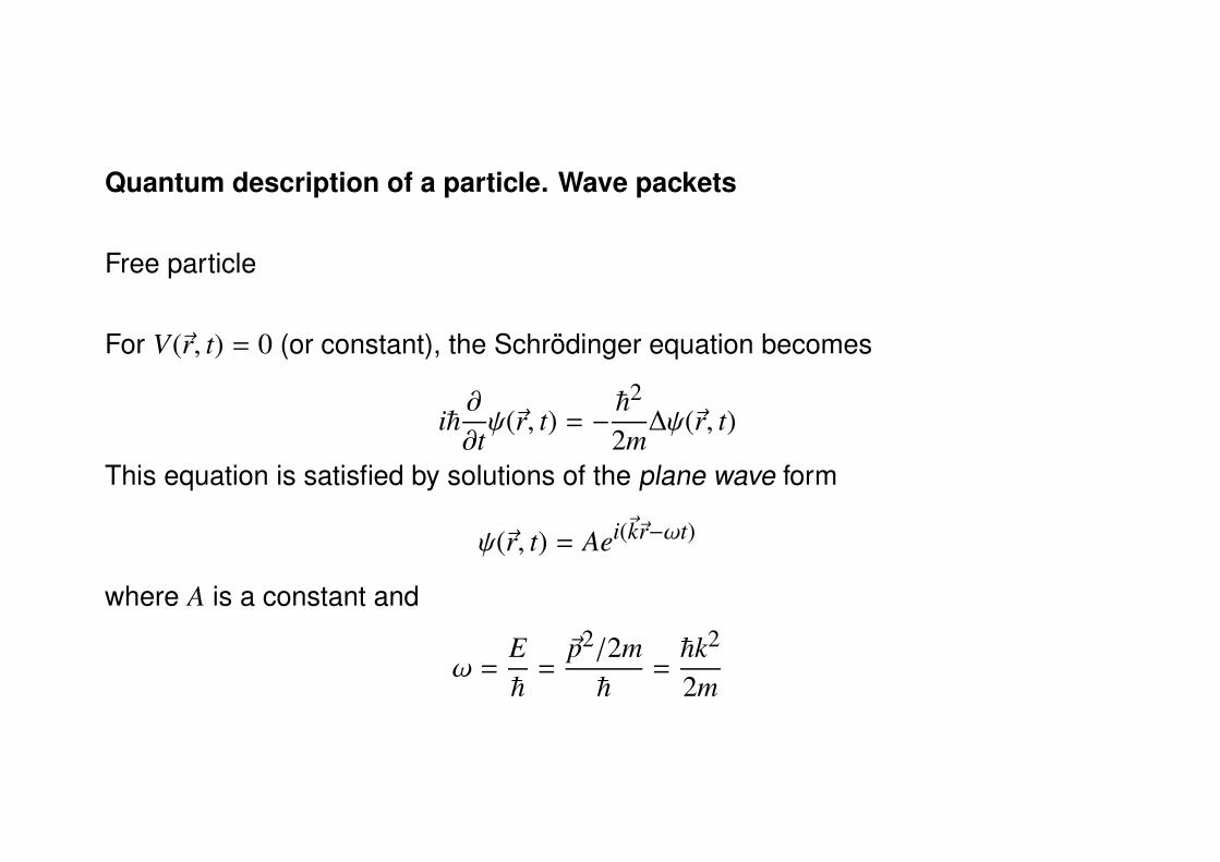
Quantum description of a particle. Wave packets

Free particle

For V(~r, t) = 0 (or constant), the Schrodinger equation becomes

i~∂

∂tψ(~r, t) = −

~2

2m∆ψ(~r, t)

This equation is satisfied by solutions of the plane wave form

ψ(~r, t) = Aei(~k~r−ωt)

where A is a constant and

ω =E~

=~p2/2m~

=~k2

2m

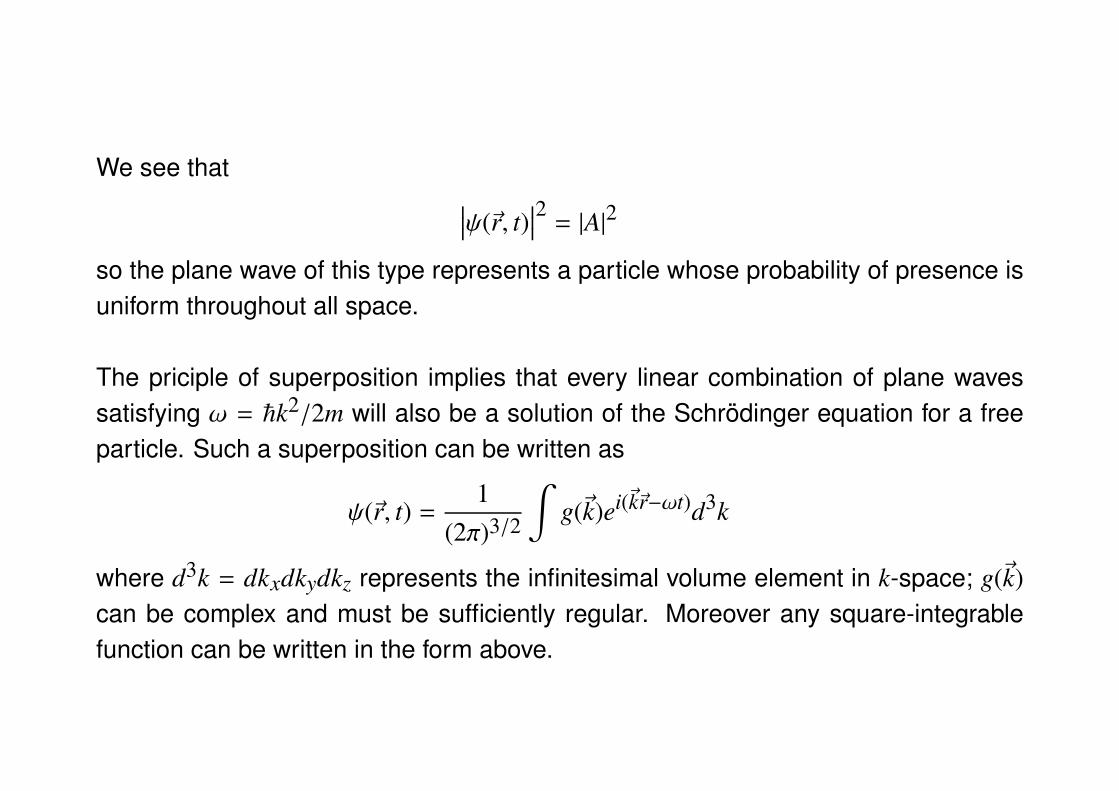
We see that ∣∣∣ψ(~r, t)∣∣∣2 = |A|2

so the plane wave of this type represents a particle whose probability of presence isuniform throughout all space.

The priciple of superposition implies that every linear combination of plane wavessatisfying ω = ~k2/2m will also be a solution of the Schrodinger equation for a freeparticle. Such a superposition can be written as

ψ(~r, t) =1

(2π)3/2

∫g(~k)ei(~k~r−ωt)d3k

where d3k = dkxdkydkz represents the infinitesimal volume element in k-space; g(~k)can be complex and must be sufficiently regular. Moreover any square-integrablefunction can be written in the form above.

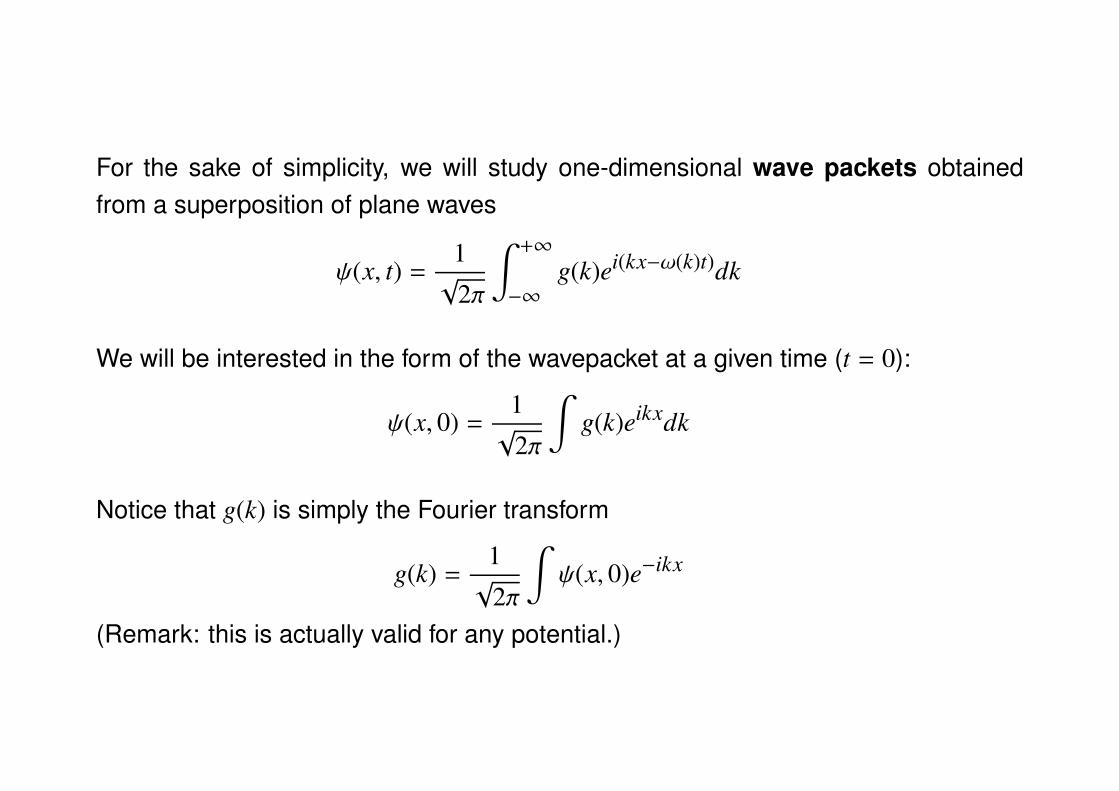
For the sake of simplicity, we will study one-dimensional wave packets obtainedfrom a superposition of plane waves

ψ(x, t) =1√

2π

∫ +∞

−∞

g(k)ei(kx−ω(k)t)dk

We will be interested in the form of the wavepacket at a given time (t = 0):

ψ(x, 0) =1√

2π

∫g(k)eikxdk

Notice that g(k) is simply the Fourier transform

g(k) =1√

2π

∫ψ(x, 0)e−ikx

(Remark: this is actually valid for any potential.)

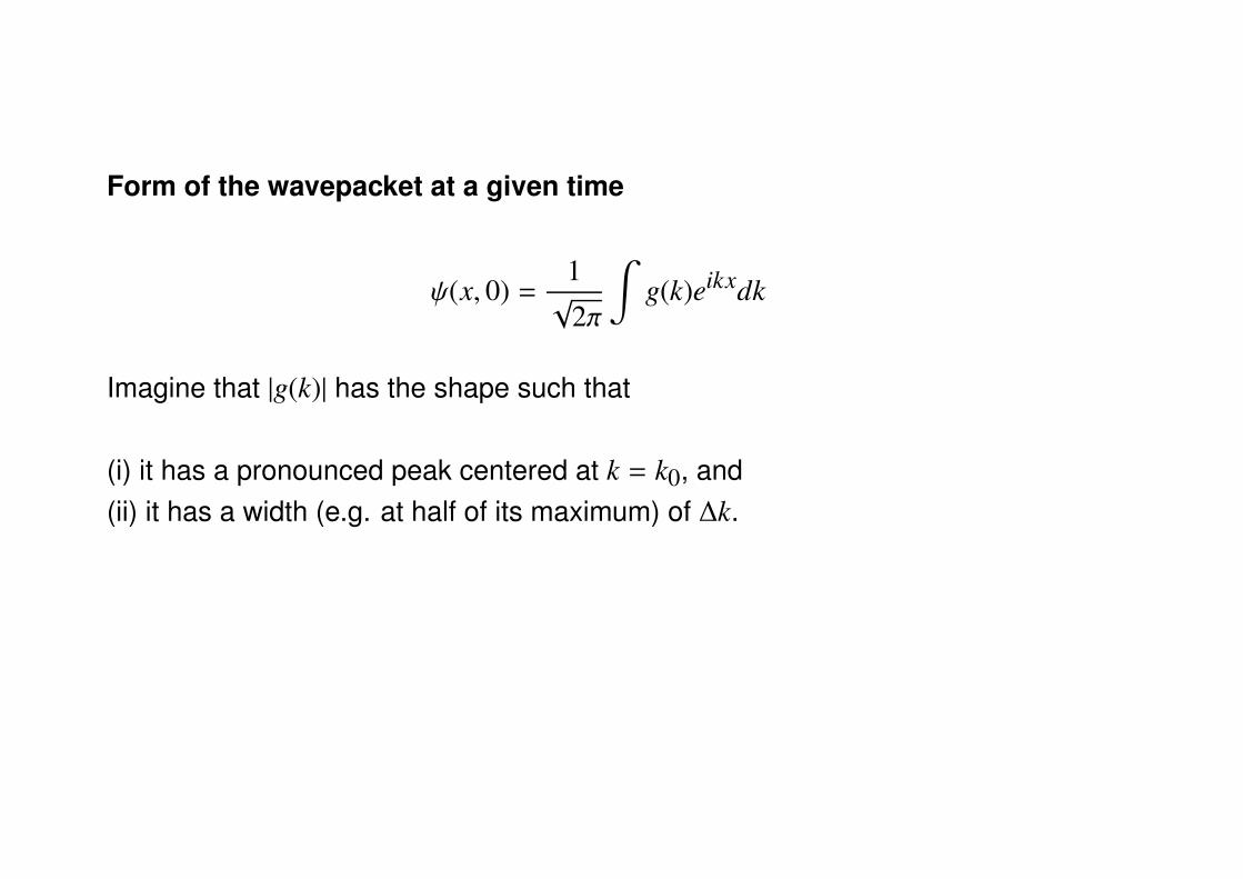
Form of the wavepacket at a given time

ψ(x, 0) =1√

2π

∫g(k)eikxdk

Imagine that |g(k)| has the shape such that

(i) it has a pronounced peak centered at k = k0, and(ii) it has a width (e.g. at half of its maximum) of ∆k.

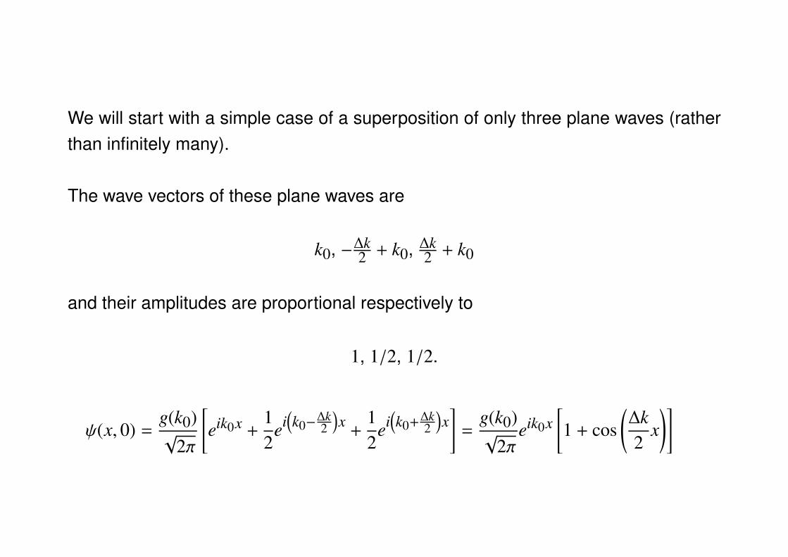
We will start with a simple case of a superposition of only three plane waves (ratherthan infinitely many).

The wave vectors of these plane waves are

k0, −∆k2 + k0, ∆k

2 + k0

and their amplitudes are proportional respectively to

1, 1/2, 1/2.

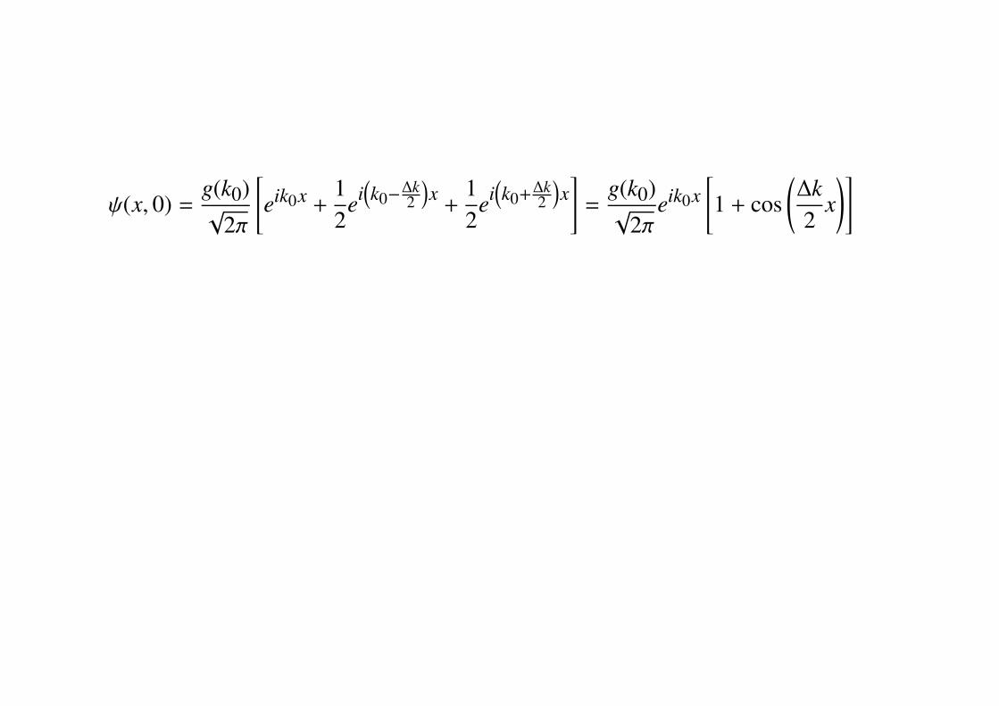
ψ(x, 0) =g(k0)√

2π

[eik0x +

12

ei(k0−

∆k2

)x

+12

ei(k0+∆k

2

)x]

=g(k0)√

2πeik0x

[1 + cos

(∆k2

x)]

ψ(x, 0) =g(k0)√

2π

[eik0x +

12

ei(k0−

∆k2

)x

+12

ei(k0+∆k

2

)x]

=g(k0)√

2πeik0x

[1 + cos

(∆k2

x)]

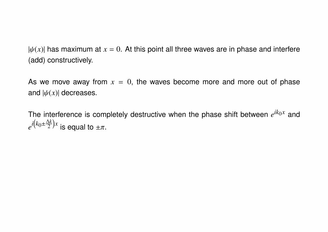
|ψ(x)| has maximum at x = 0. At this point all three waves are in phase and interfere(add) constructively.

As we move away from x = 0, the waves become more and more out of phaseand |ψ(x)| decreases.

The interference is completely destructive when the phase shift between eik0x and

ei(k0±

∆k2

)x is equal to ±π.

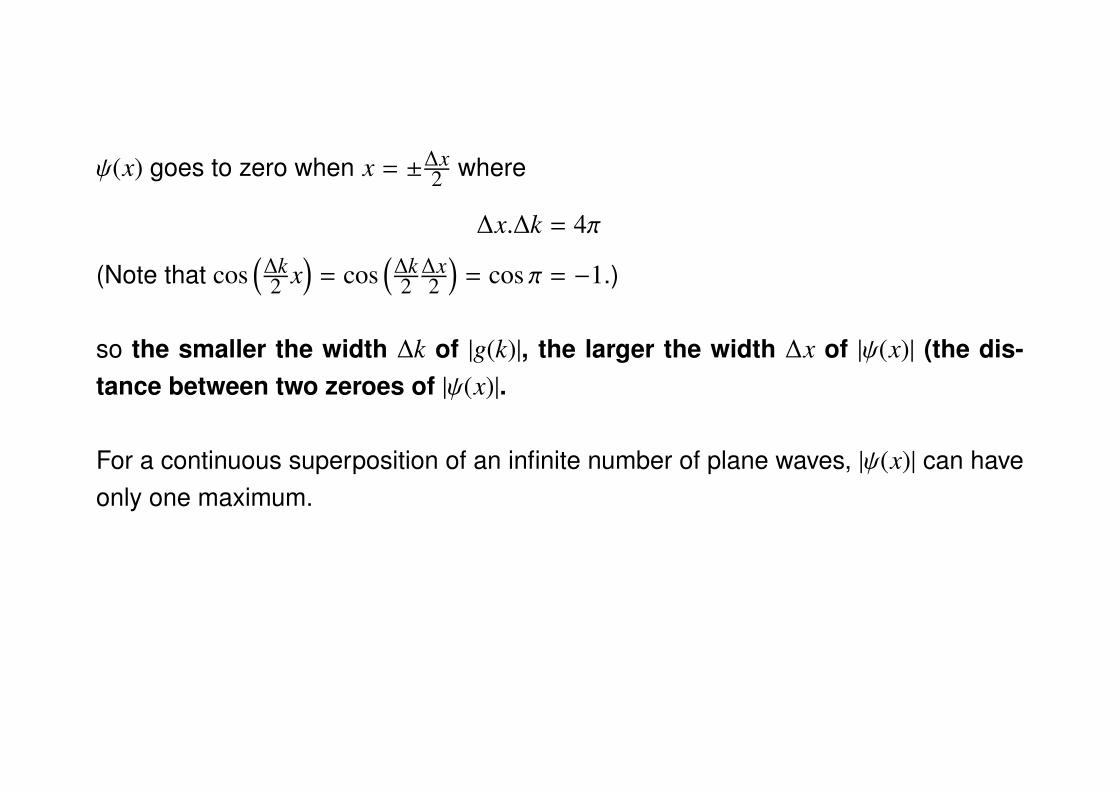
ψ(x) goes to zero when x = ±∆x2 where

∆x.∆k = 4π

(Note that cos(∆k2 x

)= cos

(∆k2

∆x2

)= cos π = −1.)

so the smaller the width ∆k of |g(k)|, the larger the width ∆x of |ψ(x)| (the dis-tance between two zeroes of |ψ(x)|.

For a continuous superposition of an infinite number of plane waves, |ψ(x)| can haveonly one maximum.

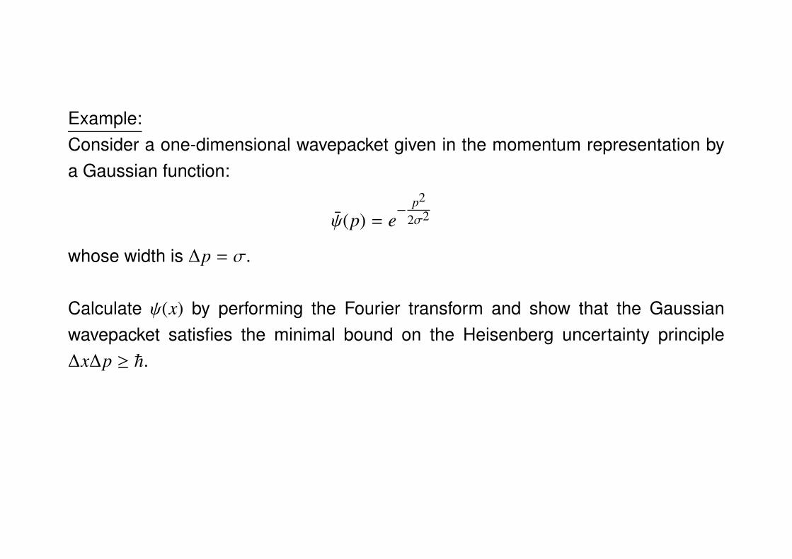
Example:Consider a one-dimensional wavepacket given in the momentum representation bya Gaussian function:

ψ(p) = e−

p2

2σ2

whose width is ∆p = σ.

Calculate ψ(x) by performing the Fourier transform and show that the Gaussianwavepacket satisfies the minimal bound on the Heisenberg uncertainty principle∆x∆p ≥ ~.

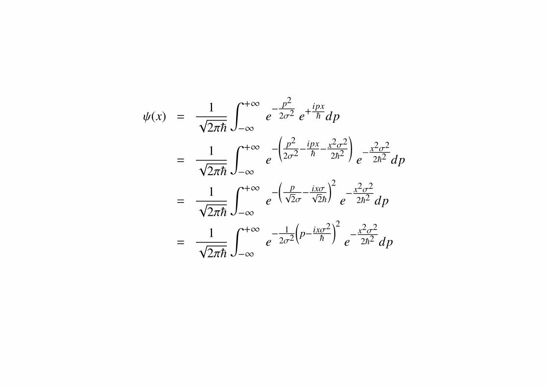
ψ(x) =1√

2π~

∫ +∞

−∞

e−

p2

2σ2 e+ipx~ dp

=1√

2π~

∫ +∞

−∞

e−

(p2

2σ2−ipx~ −

x2σ2

2~2

)e− x2σ2

2~2 dp

=1√

2π~

∫ +∞

−∞

e−

(p√

2σ− ixσ√

2~

)2

e− x2σ2

2~2 dp

=1√

2π~

∫ +∞

−∞

e− 1

2σ2

(p− ixσ2

~

)2

e− x2σ2

2~2 dp

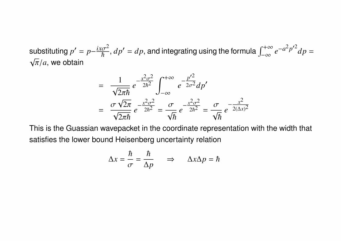
substituting p′ = p−ixσ2

~ , dp′ = dp, and integrating using the formula∫ +∞

−∞e−a2p′2dp =

√π/a, we obtain

=1√

2π~e− x2σ2

2~2∫ +∞

−∞

e−

p′2

2σ2 dp′

=σ√

2π√

2π~e− x2σ2

2~2 =σ√~

e− x2σ2

2~2 =σ√~

e− x2

2(∆x)2

This is the Guassian wavepacket in the coordinate representation with the width thatsatisfies the lower bound Heisenberg uncertainty relation

∆x =~

σ=~

∆p⇒ ∆x∆p = ~

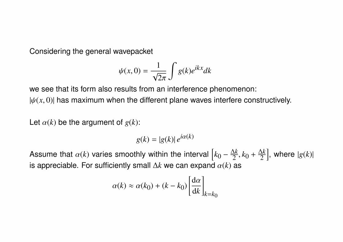
Considering the general wavepacket

ψ(x, 0) =1√

2π

∫g(k)eikxdk

we see that its form also results from an interference phenomenon:|ψ(x, 0)| has maximum when the different plane waves interfere constructively.

Let α(k) be the argument of g(k):

g(k) = |g(k)| eiα(k)

Assume that α(k) varies smoothly within the interval[k0 −

∆k2 , k0 + ∆k

2

], where |g(k)|

is appreciable. For sufficiently small ∆k we can expand α(k) as

α(k) ≈ α(k0) + (k − k0)[dαdk

]k=k0

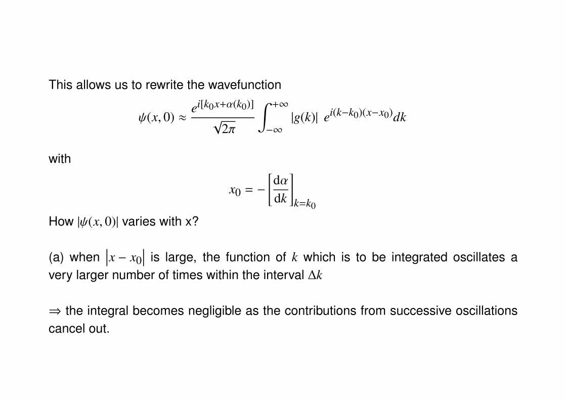
This allows us to rewrite the wavefunction

ψ(x, 0) ≈ei[k0x+α(k0)]√

2π

∫ +∞

−∞

|g(k)| ei(k−k0)(x−x0)dk

with

x0 = −

[dαdk

]k=k0

How |ψ(x, 0)| varies with x?

(a) when∣∣∣x − x0

∣∣∣ is large, the function of k which is to be integrated oscillates avery larger number of times within the interval ∆k

⇒ the integral becomes negligible as the contributions from successive oscillationscancel out.

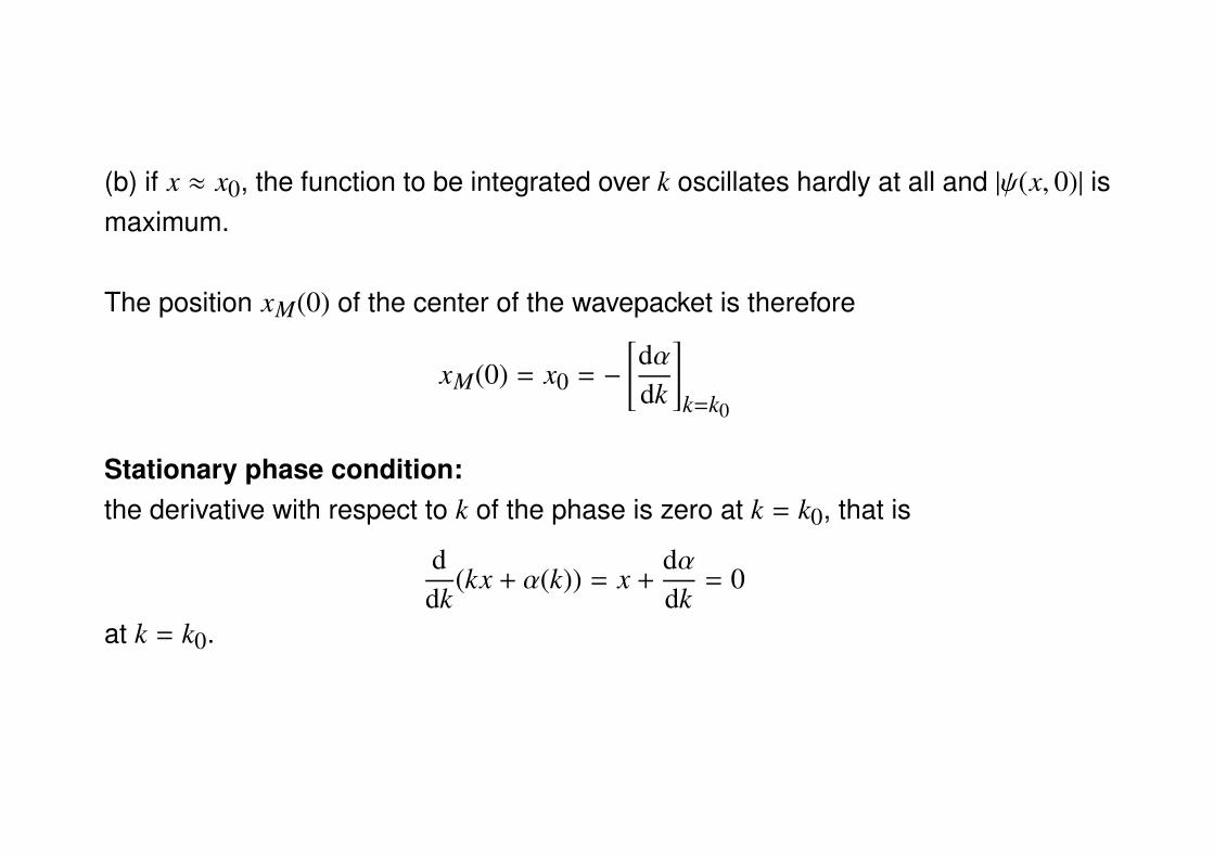
(b) if x ≈ x0, the function to be integrated over k oscillates hardly at all and |ψ(x, 0)| ismaximum.

The position xM(0) of the center of the wavepacket is therefore

xM(0) = x0 = −

[dαdk

]k=k0

Stationary phase condition:the derivative with respect to k of the phase is zero at k = k0, that is

ddk

(kx + α(k)) = x +dαdk

= 0

at k = k0.

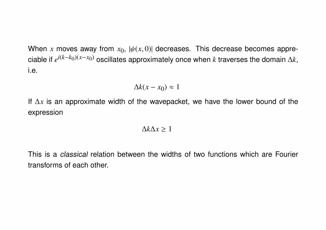
When x moves away from x0, |ψ(x, 0)| decreases. This decrease becomes appre-ciable if ei(k−k0)(x−x0) oscillates approximately once when k traverses the domain ∆k,i.e.

∆k(x − x0) ≈ 1

If ∆x is an approximate width of the wavepacket, we have the lower bound of theexpression

∆k∆x ≥ 1

This is a classical relation between the widths of two functions which are Fouriertransforms of each other.

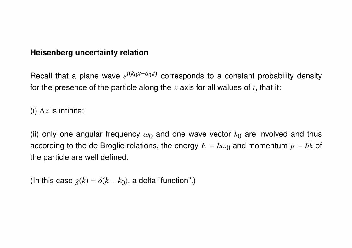
Heisenberg uncertainty relation

Recall that a plane wave ei(k0x−ω0t) corresponds to a constant probability densityfor the presence of the particle along the x axis for all walues of t, that it:

(i) ∆x is infinite;

(ii) only one angular frequency ω0 and one wave vector k0 are involved and thusaccording to the de Broglie relations, the energy E = ~ω0 and momentum p = ~k ofthe particle are well defined.

(In this case g(k) = δ(k − k0), a delta ”function”.)

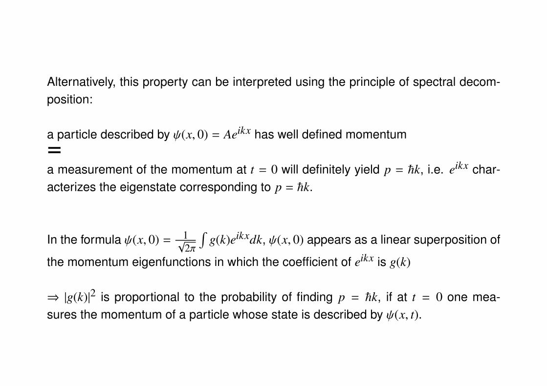
Alternatively, this property can be interpreted using the principle of spectral decom-position:

a particle described by ψ(x, 0) = Aeikx has well defined momentum=a measurement of the momentum at t = 0 will definitely yield p = ~k, i.e. eikx char-acterizes the eigenstate corresponding to p = ~k.

In the formula ψ(x, 0) = 1√2π

∫g(k)eikxdk, ψ(x, 0) appears as a linear superposition of

the momentum eigenfunctions in which the coefficient of eikx is g(k)

⇒ |g(k)|2 is proportional to the probability of finding p = ~k, if at t = 0 one mea-sures the momentum of a particle whose state is described by ψ(x, t).

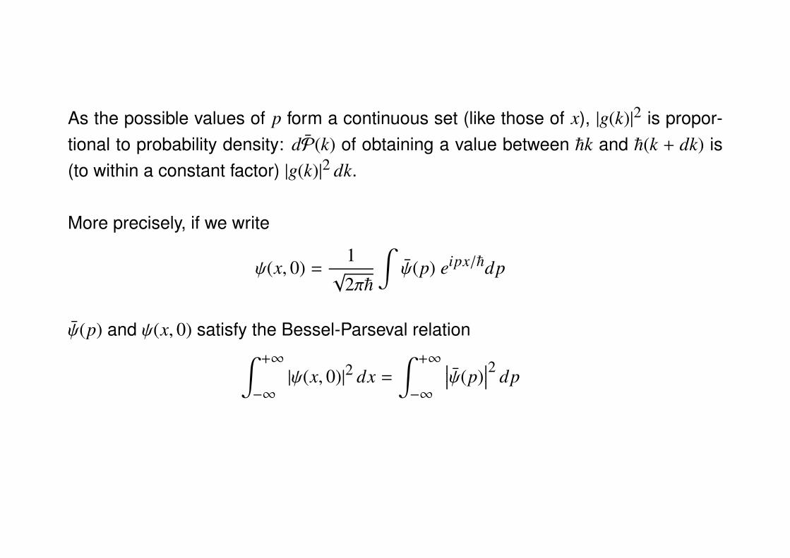
As the possible values of p form a continuous set (like those of x), |g(k)|2 is propor-tional to probability density: dP(k) of obtaining a value between ~k and ~(k + dk) is(to within a constant factor) |g(k)|2 dk.

More precisely, if we write

ψ(x, 0) =1√

2π~

∫ψ(p) eipx/~dp

ψ(p) and ψ(x, 0) satisfy the Bessel-Parseval relation∫ +∞

−∞

|ψ(x, 0)|2 dx =

∫ +∞

−∞

∣∣∣ψ(p)∣∣∣2 dp

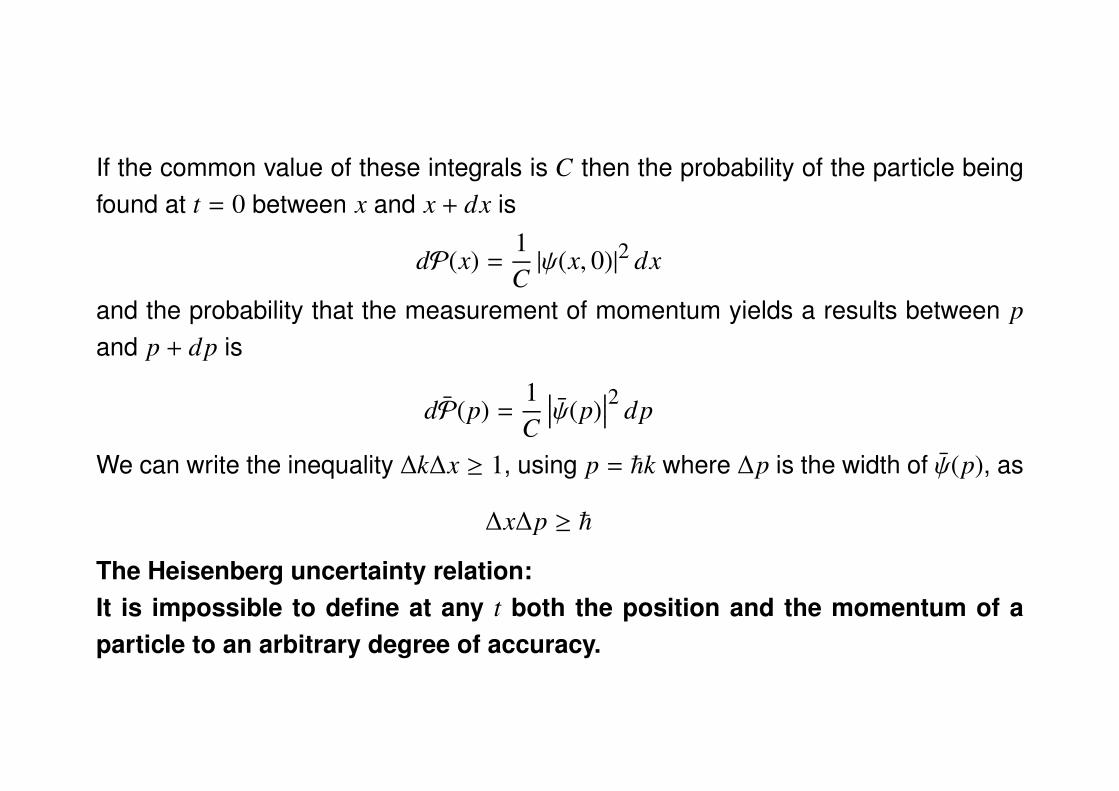
If the common value of these integrals is C then the probability of the particle beingfound at t = 0 between x and x + dx is

dP(x) =1C|ψ(x, 0)|2 dx

and the probability that the measurement of momentum yields a results between pand p + dp is

dP(p) =1C

∣∣∣ψ(p)∣∣∣2 dp

We can write the inequality ∆k∆x ≥ 1, using p = ~k where ∆p is the width of ψ(p), as

∆x∆p ≥ ~

The Heisenberg uncertainty relation:It is impossible to define at any t both the position and the momentum of aparticle to an arbitrary degree of accuracy.

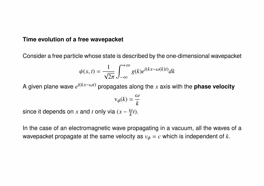
Time evolution of a free wavepacket

Consider a free particle whose state is described by the one-dimensional wavepacket

ψ(x, t) =1√

2π

∫ +∞

−∞

g(k)ei(kx−ω(k)t)dk

A given plane wave ei(kx−ωt) propagates along the x axis with the phase velocity

vφ(k) =ω

ksince it depends on x and t only via (x − ω

k t).

In the case of an electromagnetic wave propagating in a vacuum, all the waves of awavepacket propagate at the same velocity as vφ = c which is independent of k.

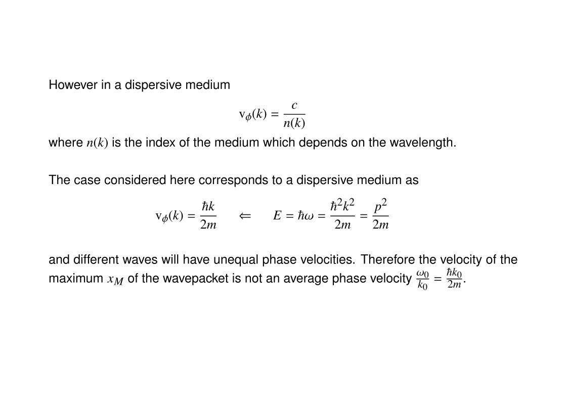
However in a dispersive medium

vφ(k) =c

n(k)where n(k) is the index of the medium which depends on the wavelength.

The case considered here corresponds to a dispersive medium as

vφ(k) =~k2m

⇐ E = ~ω =~2k2

2m=

p2

2m

and different waves will have unequal phase velocities. Therefore the velocity of themaximum xM of the wavepacket is not an average phase velocity ω0

k0=~k02m .

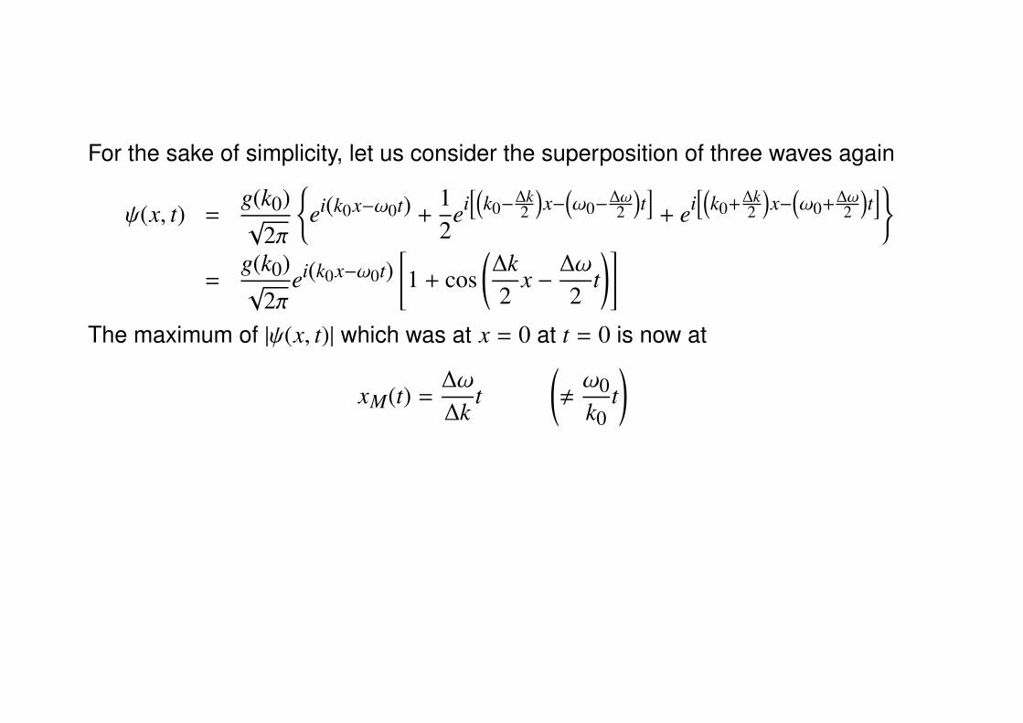
For the sake of simplicity, let us consider the superposition of three waves again

ψ(x, t) =g(k0)√

2π

{ei(k0x−ω0t) +

12

ei[(

k0−∆k2

)x−

(ω0−

∆ω2

)t]+ ei

[(k0+∆k

2

)x−

(ω0+∆ω

2

)t]}

=g(k0)√

2πei(k0x−ω0t)

[1 + cos

(∆k2

x −∆ω

2t)]

The maximum of |ψ(x, t)| which was at x = 0 at t = 0 is now at

xM(t) =∆ω

∆kt

(,ω0k0

t)

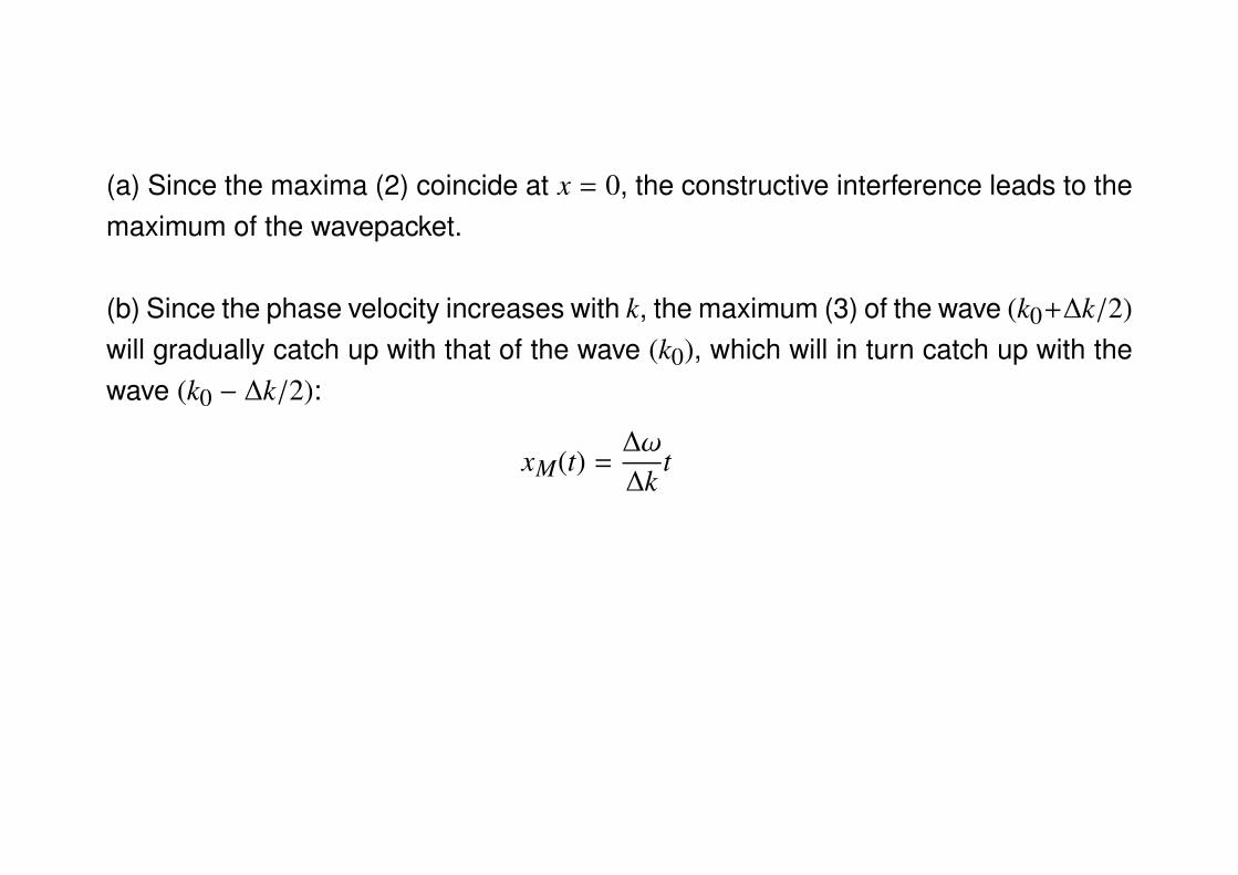
(a) Since the maxima (2) coincide at x = 0, the constructive interference leads to themaximum of the wavepacket.

(b) Since the phase velocity increases with k, the maximum (3) of the wave (k0+∆k/2)will gradually catch up with that of the wave (k0), which will in turn catch up with thewave (k0 − ∆k/2):

xM(t) =∆ω

∆kt

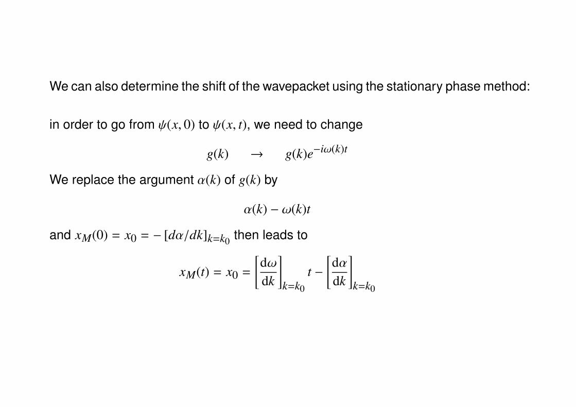
We can also determine the shift of the wavepacket using the stationary phase method:

in order to go from ψ(x, 0) to ψ(x, t), we need to change

g(k) → g(k)e−iω(k)t

We replace the argument α(k) of g(k) by

α(k) − ω(k)t

and xM(0) = x0 = − [dα/dk]k=k0 then leads to

xM(t) = x0 =

[dωdk

]k=k0

t −[dαdk

]k=k0

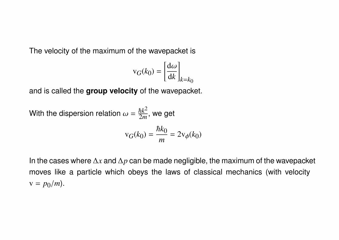
The velocity of the maximum of the wavepacket is

vG(k0) =

[dωdk

]k=k0

and is called the group velocity of the wavepacket.

With the dispersion relation ω = ~k2

2m , we get

vG(k0) =~k0m

= 2vφ(k0)

In the cases where ∆x and ∆p can be made negligible, the maximum of the wavepacketmoves like a particle which obeys the laws of classical mechanics (with velocityv = p0/m).

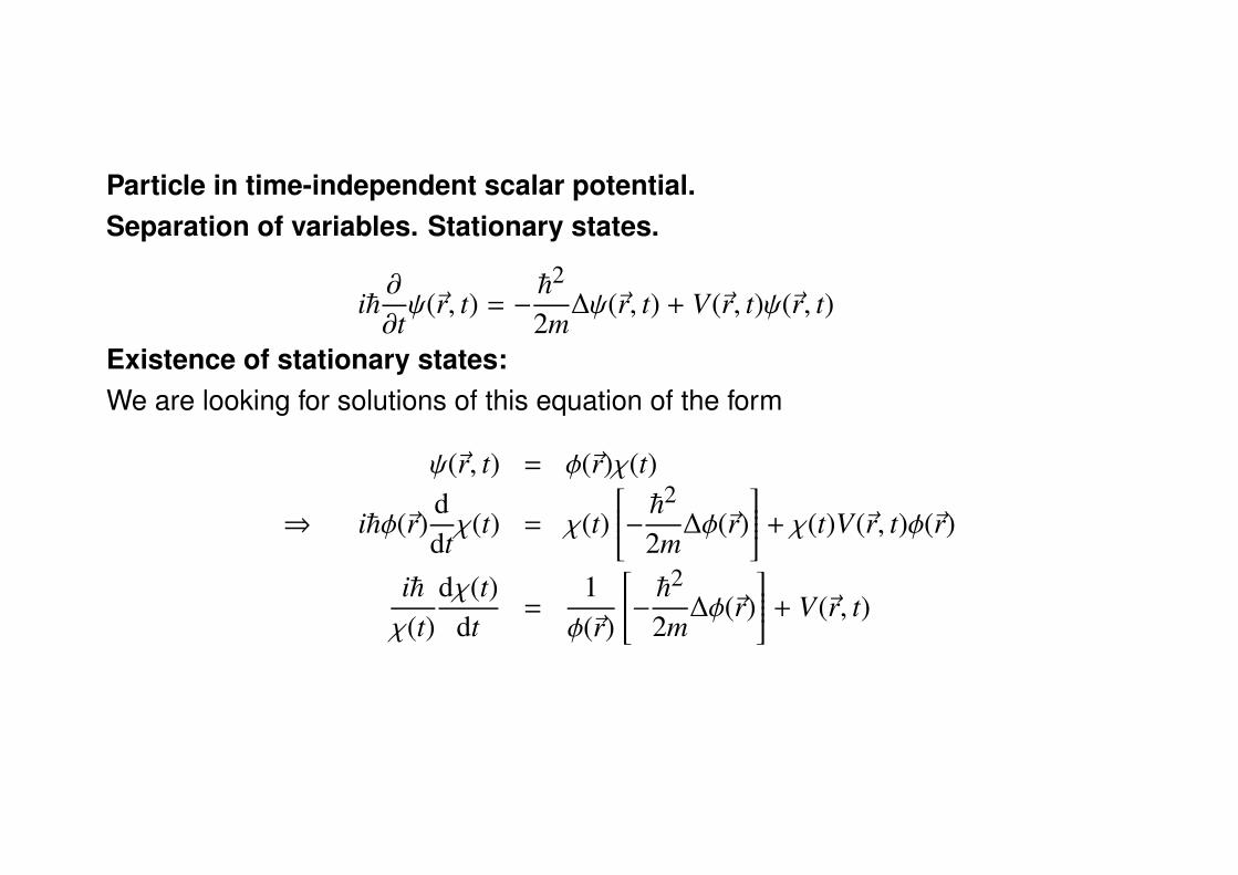
Particle in time-independent scalar potential.Separation of variables. Stationary states.

i~∂

∂tψ(~r, t) = −

~2

2m∆ψ(~r, t) + V(~r, t)ψ(~r, t)

Existence of stationary states:We are looking for solutions of this equation of the form

ψ(~r, t) = φ(~r)χ(t)

⇒ i~φ(~r)ddtχ(t) = χ(t)

− ~22m∆φ(~r)

+ χ(t)V(~r, t)φ(~r)

i~χ(t)

dχ(t)dt

=1φ(~r)

− ~22m∆φ(~r)

+ V(~r, t)

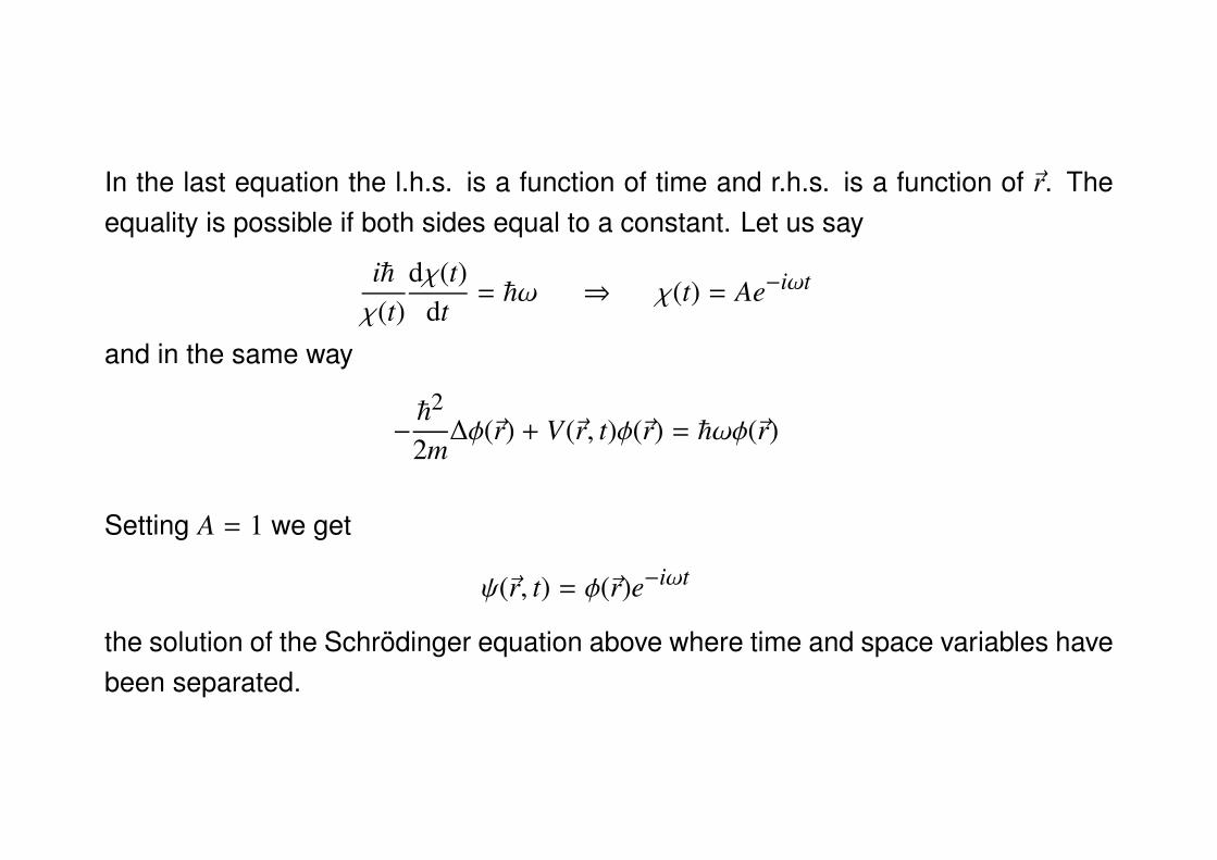
In the last equation the l.h.s. is a function of time and r.h.s. is a function of ~r. Theequality is possible if both sides equal to a constant. Let us say

i~χ(t)

dχ(t)dt

= ~ω ⇒ χ(t) = Ae−iωt

and in the same way

−~2

2m∆φ(~r) + V(~r, t)φ(~r) = ~ωφ(~r)

Setting A = 1 we get

ψ(~r, t) = φ(~r)e−iωt

the solution of the Schrodinger equation above where time and space variables havebeen separated.

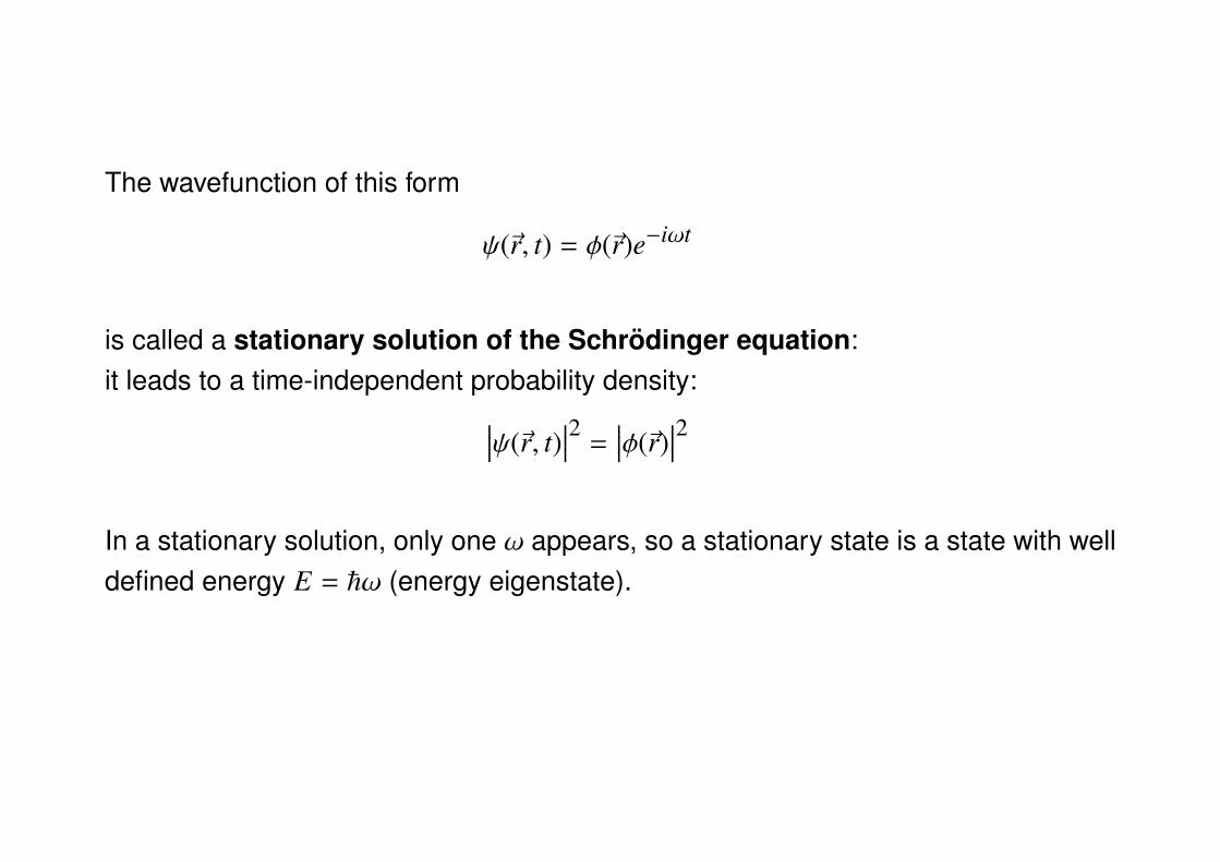
The wavefunction of this form

ψ(~r, t) = φ(~r)e−iωt

is called a stationary solution of the Schrodinger equation:it leads to a time-independent probability density:∣∣∣ψ(~r, t)

∣∣∣2 =∣∣∣φ(~r)

∣∣∣2In a stationary solution, only one ω appears, so a stationary state is a state with welldefined energy E = ~ω (energy eigenstate).

Provided the potential energy is time independent

(i) in classical mechanics, the total energy is a constant of motion;

(ii) in quantum mechanics, there exist well-defined energy states:− ~22m∆ + V(~r, t)

φ(~r) = Eφ(~r)

or

Hφ(~r) = Eφ(~r)

This is the eigenvalue equation for the Hamiltonian, the differential operator rep-resenting the total energy. E is the eigenvalue (total energy) and φ(~r) is the corre-sponding eigenvector (the eigenvalue equation reflects energy quantization).The Hamiltonian is a linear operator, that is H[λ1φ1 + λ2φ2] = λ1Hφ1 + λ2Hφ2.

Superposition of stationary states

We label various energy values by an index n:

Hφn(~r) = Enφn(~r)

where the stationary states are

ψn(~r, t) = φn(~r)e−iEnt/~

The Schrodinger equation, as a linear equation, has a whole series of solutions ofthe form

ψ(~r, t) =∑

ncnφn(~r)e−iEnt/~

where cn are complex numbers. In particular

ψ(~r, 0) =∑

ncnφn(~r)

Any function ψ(~r, 0) can always be decomposed in terms of eigenfunctions of H. Thecoefficients cn are thus always determined by ψ(~r, 0).

The states time-dependence arises from the terms e−iEnt/~ where En is the eigen-value associated with the eigenvector (eigenstate) φn(~r).

Stationary states of a particle in one-dimensional square potentials

Behavior of a stationary wavefunction φ(x):

d2

dx2φ(x) +2m~2

(E − V) φ(x) = 0

where V(x) = V in some region of space.

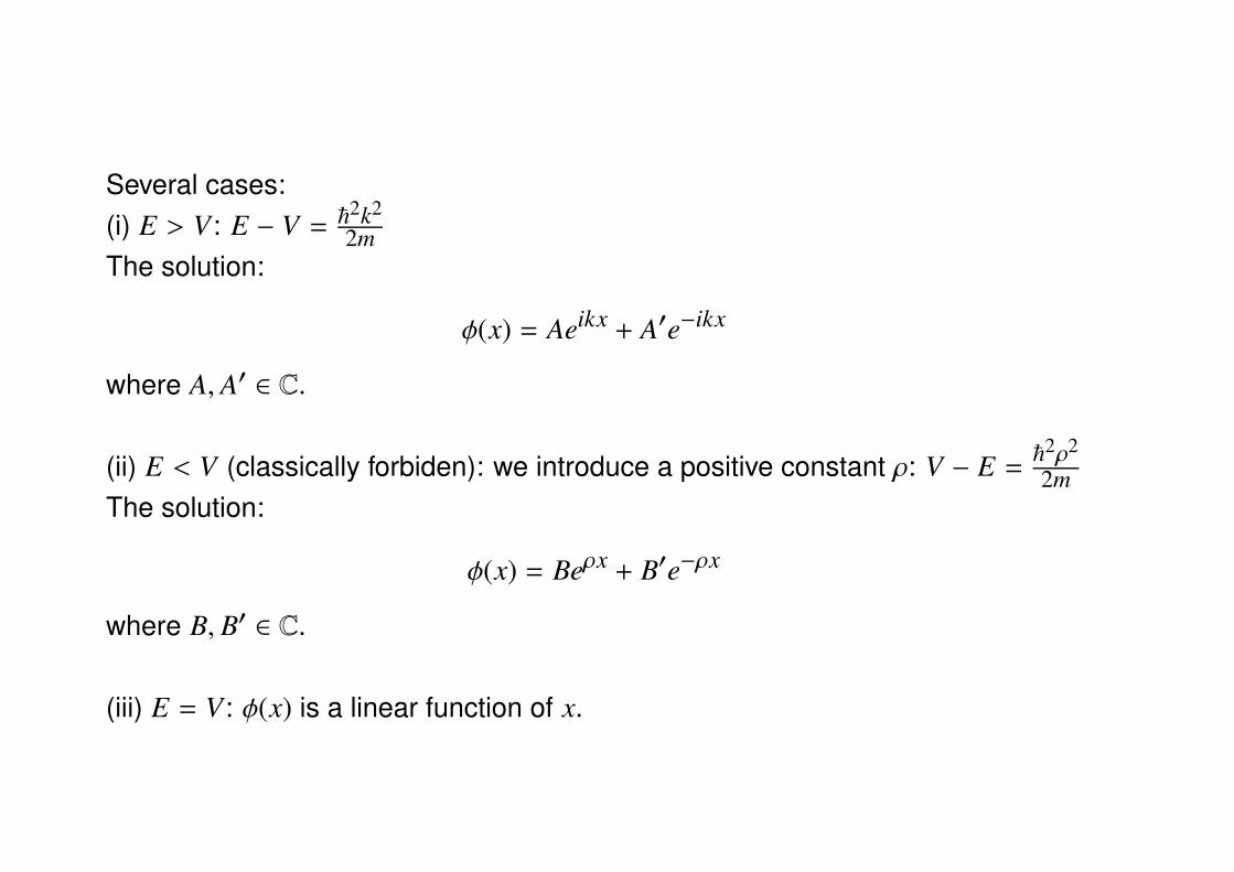
Several cases:(i) E > V: E − V = ~

2k2

2mThe solution:

φ(x) = Aeikx + A′e−ikx

where A, A′ ∈ C.

(ii) E < V (classically forbiden): we introduce a positive constant ρ: V − E =~2ρ2

2mThe solution:

φ(x) = Beρx + B′e−ρx

where B, B′ ∈ C.

(iii) E = V: φ(x) is a linear function of x.

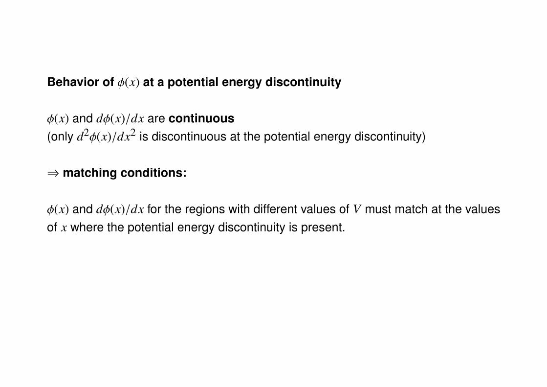
Behavior of φ(x) at a potential energy discontinuity

φ(x) and dφ(x)/dx are continuous(only d2φ(x)/dx2 is discontinuous at the potential energy discontinuity)

⇒ matching conditions:

φ(x) and dφ(x)/dx for the regions with different values of V must match at the valuesof x where the potential energy discontinuity is present.

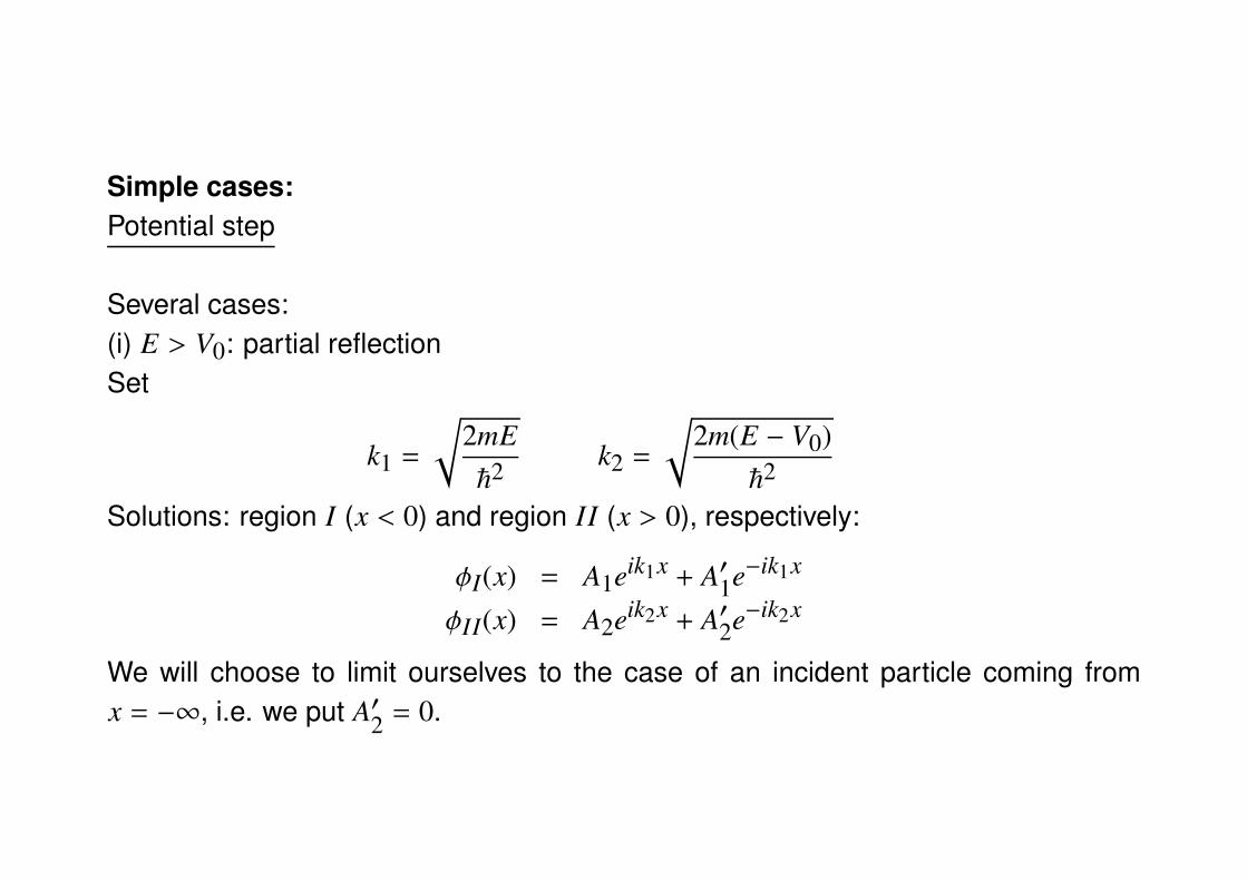
Simple cases:Potential step

Several cases:(i) E > V0: partial reflectionSet

k1 =

√2mE~2

k2 =

√2m(E − V0)~2

Solutions: region I (x < 0) and region II (x > 0), respectively:

φI(x) = A1eik1x + A′1e−ik1x

φII(x) = A2eik2x + A′2e−ik2x

We will choose to limit ourselves to the case of an incident particle coming fromx = −∞, i.e. we put A′2 = 0.

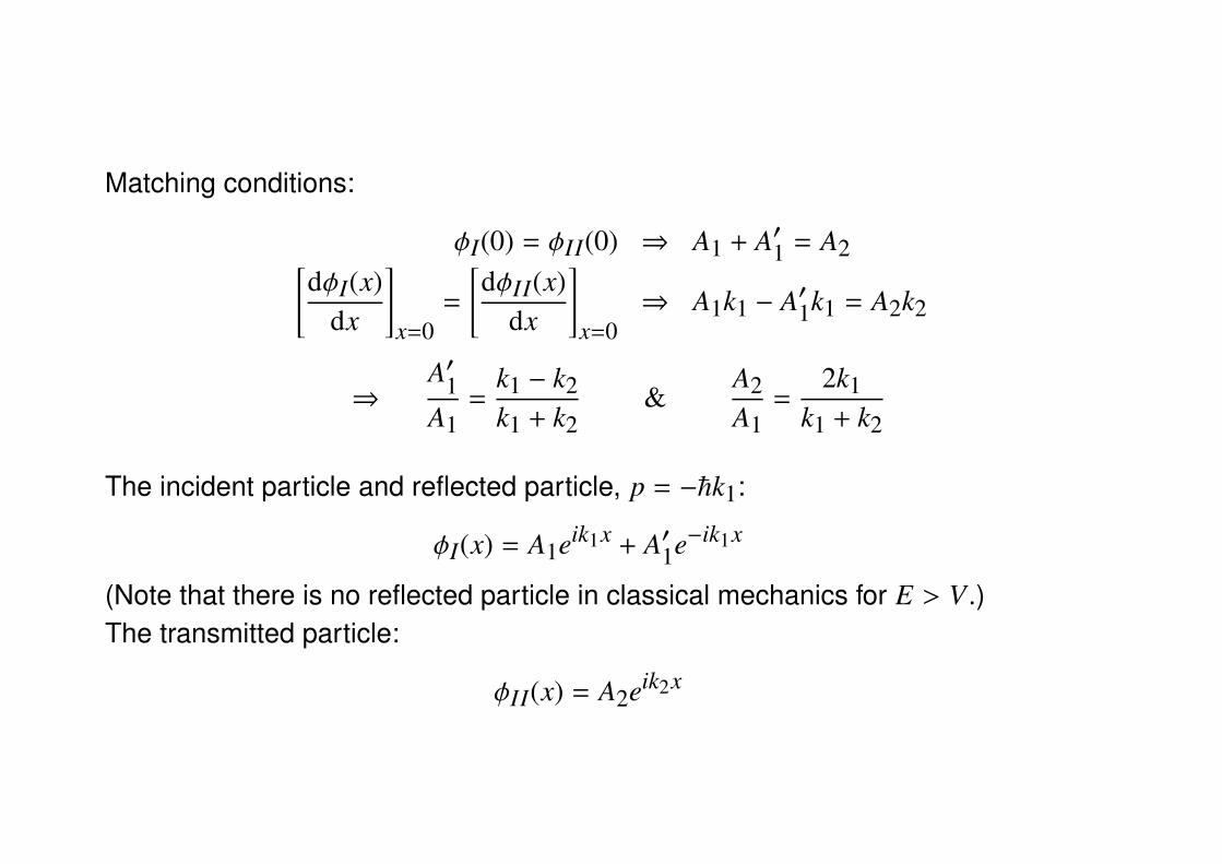
Matching conditions:

φI(0) = φII(0) ⇒ A1 + A′1 = A2[dφI(x)

dx

]x=0

=

[dφII(x)

dx

]x=0

⇒ A1k1 − A′1k1 = A2k2

⇒A′1A1

=k1 − k2k1 + k2

&A2A1

=2k1

k1 + k2

The incident particle and reflected particle, p = −~k1:

φI(x) = A1eik1x + A′1e−ik1x

(Note that there is no reflected particle in classical mechanics for E > V.)The transmitted particle:

φII(x) = A2eik2x

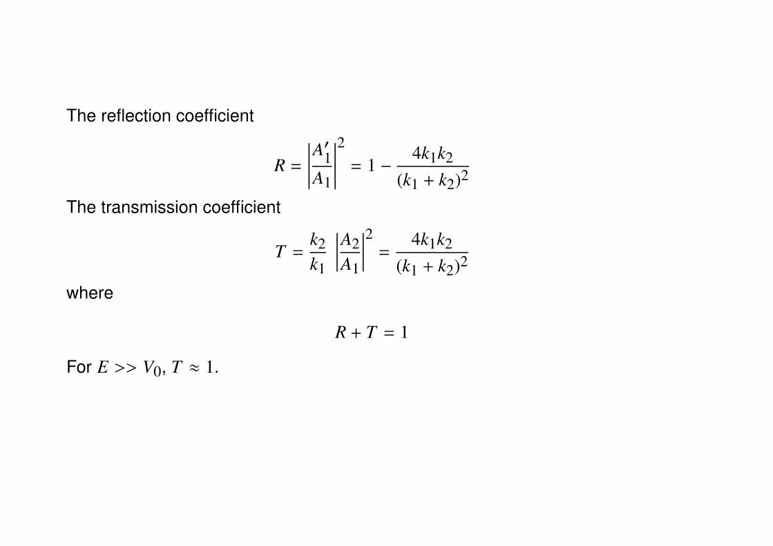
The reflection coefficient

R =

∣∣∣∣∣∣A′1A1

∣∣∣∣∣∣2

= 1 −4k1k2

(k1 + k2)2

The transmission coefficient

T =k2k1

∣∣∣∣∣A2A1

∣∣∣∣∣2 =4k1k2

(k1 + k2)2

where

R + T = 1

For E >> V0, T ≈ 1.

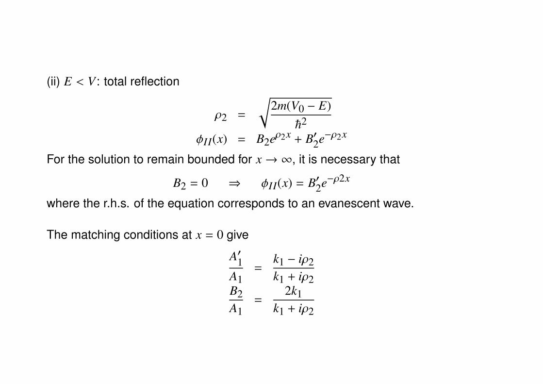
(ii) E < V: total reflection

ρ2 =

√2m(V0 − E)~2

φII(x) = B2eρ2x + B′2e−ρ2x

For the solution to remain bounded for x→ ∞, it is necessary that

B2 = 0 ⇒ φII(x) = B′2e−ρ2x

where the r.h.s. of the equation corresponds to an evanescent wave.

The matching conditions at x = 0 give

A′1A1

=k1 − iρ2k1 + iρ2

B2A1

=2k1

k1 + iρ2

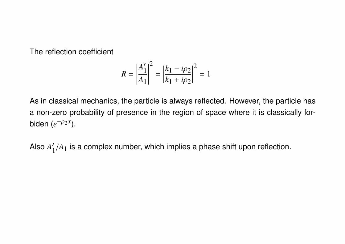
The reflection coefficient

R =

∣∣∣∣∣∣A′1A1

∣∣∣∣∣∣2

=

∣∣∣∣∣k1 − iρ2k1 + iρ2

∣∣∣∣∣2 = 1

As in classical mechanics, the particle is always reflected. However, the particle hasa non-zero probability of presence in the region of space where it is classically for-biden (e−ρ2x).

Also A′1/A1 is a complex number, which implies a phase shift upon reflection.

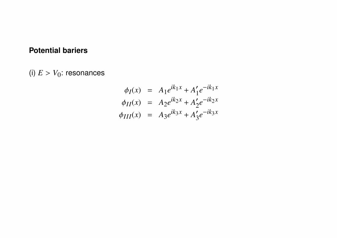
Potential bariers

(i) E > V0: resonances

φI(x) = A1eik1x + A′1e−ik1x

φII(x) = A2eik2x + A′2e−ik2x

φIII(x) = A3eik3x + A′3e−ik3x

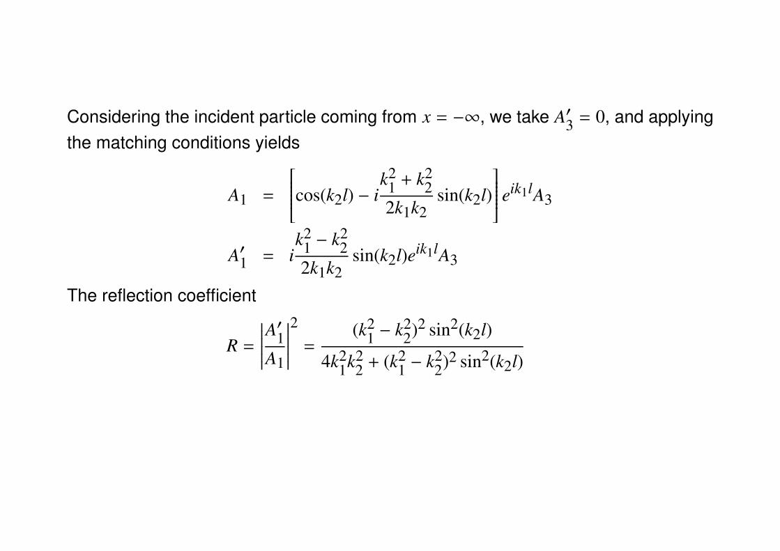
Considering the incident particle coming from x = −∞, we take A′3 = 0, and applyingthe matching conditions yields

A1 =

cos(k2l) − ik2

1 + k22

2k1k2sin(k2l)

eik1lA3

A′1 = ik2

1 − k22

2k1k2sin(k2l)eik1lA3

The reflection coefficient

R =

∣∣∣∣∣∣A′1A1

∣∣∣∣∣∣2

=(k2

1 − k22)2 sin2(k2l)

4k21k2

2 + (k21 − k2

2)2 sin2(k2l)

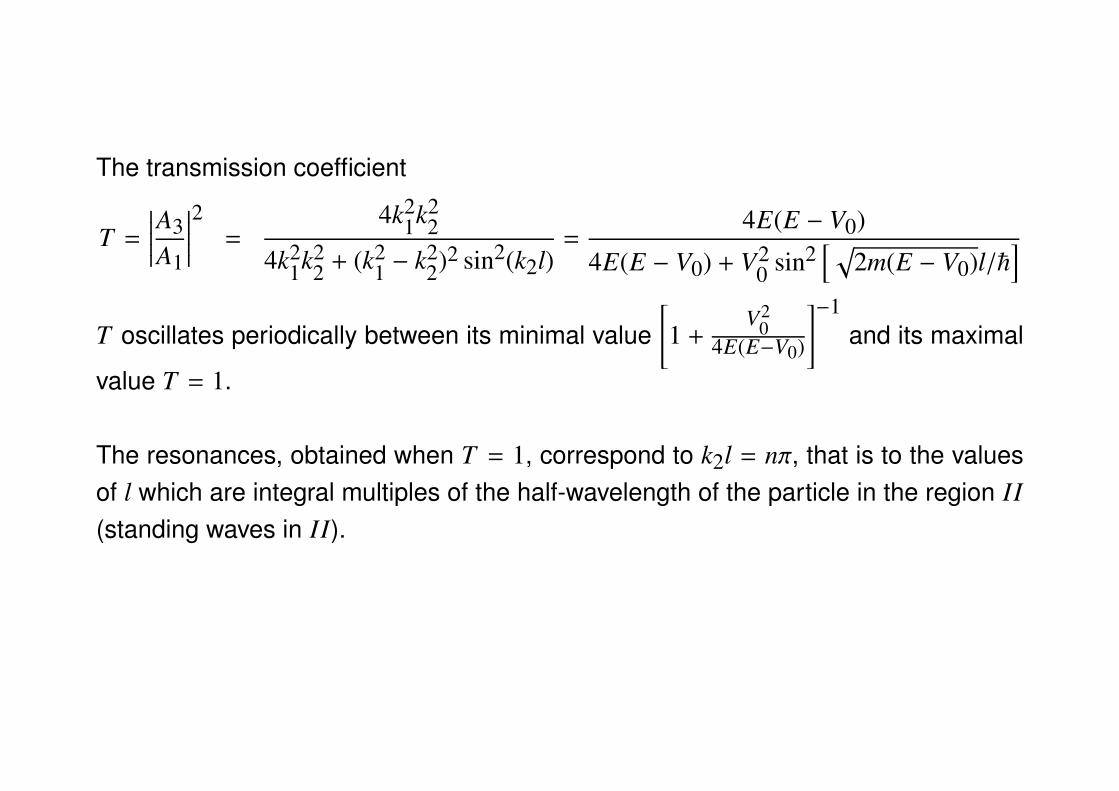
The transmission coefficient

T =

∣∣∣∣∣A3A1

∣∣∣∣∣2 =4k2

1k22

4k21k2

2 + (k21 − k2

2)2 sin2(k2l)=

4E(E − V0)

4E(E − V0) + V20 sin2

[ √2m(E − V0)l/~

]T oscillates periodically between its minimal value

[1 +

V20

4E(E−V0)

]−1and its maximal

value T = 1.

The resonances, obtained when T = 1, correspond to k2l = nπ, that is to the valuesof l which are integral multiples of the half-wavelength of the particle in the region II(standing waves in II).

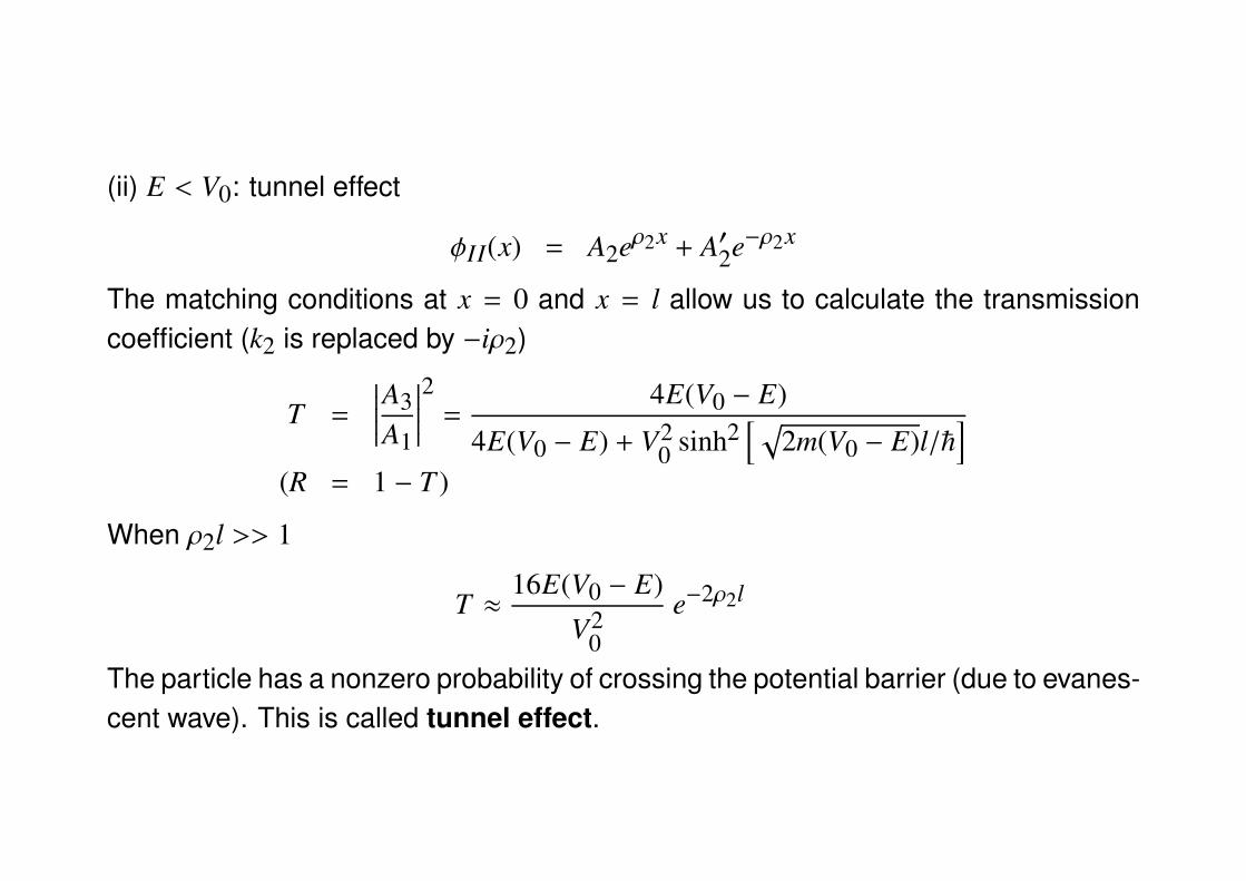
(ii) E < V0: tunnel effect

φII(x) = A2eρ2x + A′2e−ρ2x

The matching conditions at x = 0 and x = l allow us to calculate the transmissioncoefficient (k2 is replaced by −iρ2)

T =

∣∣∣∣∣A3A1

∣∣∣∣∣2 =4E(V0 − E)

4E(V0 − E) + V20 sinh2

[ √2m(V0 − E)l/~

](R = 1 − T )

When ρ2l >> 1

T ≈16E(V0 − E)

V20

e−2ρ2l

The particle has a nonzero probability of crossing the potential barrier (due to evanes-cent wave). This is called tunnel effect.

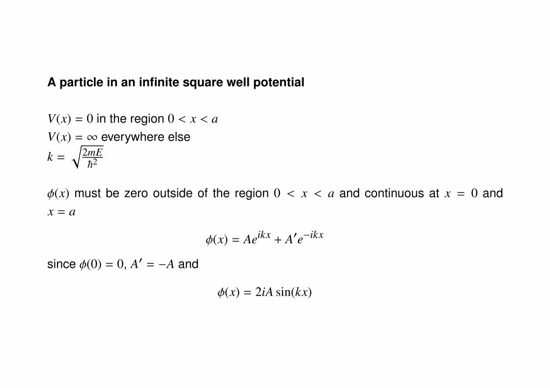
A particle in an infinite square well potential

V(x) = 0 in the region 0 < x < aV(x) = ∞ everywhere else

k =√

2mE~2

φ(x) must be zero outside of the region 0 < x < a and continuous at x = 0 andx = a

φ(x) = Aeikx + A′e−ikx

since φ(0) = 0, A′ = −A and

φ(x) = 2iA sin(kx)

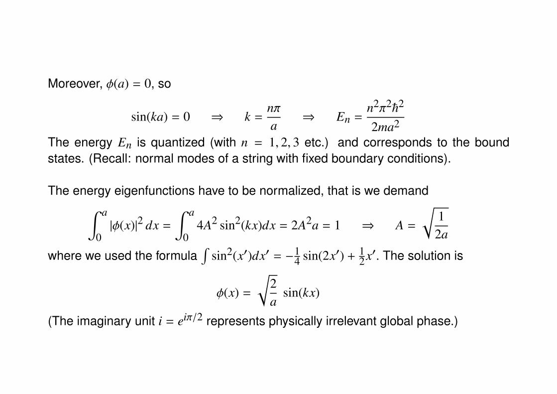
Moreover, φ(a) = 0, so

sin(ka) = 0 ⇒ k =nπa

⇒ En =n2π2~2

2ma2

The energy En is quantized (with n = 1, 2, 3 etc.) and corresponds to the boundstates. (Recall: normal modes of a string with fixed boundary conditions).

The energy eigenfunctions have to be normalized, that is we demand∫ a

0|φ(x)|2 dx =

∫ a

04A2 sin2(kx)dx = 2A2a = 1 ⇒ A =

√12a

where we used the formula∫

sin2(x′)dx′ = −14 sin(2x′) + 1

2x′. The solution is

φ(x) =

√2a

sin(kx)

(The imaginary unit i = eiπ/2 represents physically irrelevant global phase.)