Embed Size (px)
Citation preview

Active Learning for Visual Question Answering:
An Empirical Study
Xiao Lin Devi Parikh
Virginia Tech Georgia Tech
[email protected] [email protected]
Abstract
We present an empirical study of active learning for Visual Question Answering, where a deep VQA
model selects informative question-image pairs from a pool and queries an oracle for answers to maximally
improve its performance under a limited query budget. Drawing analogies from human learning, we
explore cramming (entropy), curiosity-driven (expected model change), and goal-driven (expected error
reduction) active learning approaches, and propose a new goal-driven active learning scoring function
to pick question-image pairs for deep VQA models under the Bayesian Neural Network framework. We
find that deep VQA models need large amounts of training data before they can start asking informative
questions. But once they do, all three approaches outperform the random selection baseline and achieve
significant query savings. For the scenario where the model is allowed to ask generic questions about
images but is evaluated only on specific questions (e.g., questions whose answer is either yes or no), our
proposed goal-driven scoring function performs the best.
1 Introduction
Visual Question Answering (VQA) [1, 8, 9, 11, 23, 28] is the task of taking in an image and a free-form
natural language question and automatically answering the question. Correctly answering VQA questions
arguably demonstrates machines’ image understanding, language understanding and and perhaps even some
commonsense reasoning abilities. Previous works have demonstrated that deep models which combine image,
question and answer representations, and are trained on large corpora of VQA data are effective at the VQA
task.
Although such deep models are often deemed data-hungry, the flip-side is that their performance scales well
with more training data. In Fig.1 we plot performance versus training set size of two representative deep
VQA models: LSTM+CNN [20] and HieCoAtt [21] trained on random subsets of the VQA v1.0 dataset [1].
We see that for both methods, accuracy improves significantly – by 12% – with every order of magnitude
of more training data. As performance improvements still seem linear, it is reasonable to expect another
12% increase by collecting a VQA dataset 10 times larger. Such trends are invariant to choice of image
feature [15] and is also observed in ImageNet image classification [24]. Note that improvements brought by
additional training data may be orthogonal to improvements in model architecture.
1
arX
iv:1
711.
0173
2v1
[cs
.CV
] 6
Nov
201
7

Figure 1: Performance of two representative VQA models: LSTM+CNN [20] and HieCoAtt [21] on random
subsets of the VQA v1.0 dataset. Both models improve by 12% with every order of magnitude of more
training data.
0.25
0.3
0.35
0.4
0.45
0.5
0.55
0.6
1000 10000 100000
VQ
A A
ccu
racy
Training Set Size
LSTM+CNN HieCoAtt
(Lu et al. 2015) (Lu et al. 2016)
However, collecting large quantities of annotated data is expensive. Even worse, as a result of long tail
distributions, it will likely result in redundant questions and answers while still having insufficient training
data for rare concepts. This is especially important for learning commonsense knowledge, as it is well known
that humans tend to talk about unusual circumstances more often than commonsense knowledge which can
be boring to talk about [10]. Active learning helps address these issues. In active learning, a model is
first trained on an initial training set. It then iteratively expands its training set by selecting potentially
informative examples according to a query strategy, and seeking annotations on these examples. Previous
works have shown that a carefully designed query strategy effectively reduces annotation effort required in a
variety of tasks for shallow models. For deep models however, active learning literature is scarce and mainly
focuses on classical unimodal tasks such as image and text classification.
In this work we study active learning for deep VQA models. VQA poses several unique challenges and
opportunities for active learning.
First, VQA is a multimodal problem. Deep VQA models may combine Multi-Layer Perceptrons (MLPs),
Convolutional Neural Nets (CNNs), Recurrent Neural Nets (RNNs) and even attention mechanisms to solve
VQA. Such models are much more complex than MLPs or CNNs alone studied in existing active learning
literature and need tailored query strategies.
Second, VQA questions are free-form and open-ended. In fact, VQA can play several roles from answering
any generic question about an image, to answering only specific question types (e.g., questions with “yes/no”
answers, or counting questions), to being a submodule in some other task (e.g., image captioning as in [19]).
Each of these different scenarios may require a different active learning approach.
Finally, VQA can be thought of as a Visual Turing Test [9] for computer vision systems. To answer questions
2

such as “does this person have 20/20 vision” and “will the cat be able to jump onto the shelf”, the computer
not only needs to understand the surface meaning of the image and the question, but it also needs to have
sufficient commonsense knowledge about our world. One could argue that proposing informative questions
about images is also a test of commonsense knowledge and intelligence.
We draw coarse analogies to human learning and explore three types of information-theoretic active learning
query strategies:
Cramming – maximizing information gain in the training domain. The objective of this strategy is
to efficiently memorize knowledge in an unlabeled pool of examples. This strategy selects unlabeled examples
whose label the model is most uncertain about (maximum entropy).
Curiosity-driven learning – maximizing information gain in model space. The objective of this
strategy is to select examples that could potentially change the belief on the model’s parameters (also known
as expected model change). There might exist examples in the pool whose labels have high uncertainty but
the model does not have enough capacity to capture them. In curiosity-driven learning the model will skip
these examples. BALD [7, 13] is one such strategy for deep models, where examples are selected to maximize
the reduction in entropy over model parameter space.
Goal-driven learning – maximizing information gain in the target domain. The objective of this
strategy is to gather knowledge to better achieve a particular goal (also known as expected error reduction).
To give an example from image classification, if the goal is to recognize digits i.e., the target domain is digit
classification, dog images in the unlabeled pool are not relevant even though their labels might be uncertain
or might change model parameters significantly. On the other hand, in addition to digit labels, some other
non-digit labels such as the orientation of the image might be useful to the digit classification task. We
propose a novel goal-driven query strategy that computes mutual information between pool questions and
test questions under the Bayesian Neural Network [2, 6] framework.
We evaluate active learning performance on VQA v1.0 [1] and v2.0 [11] under the pool-based active learning
setting described in Section 3. We show that active learning for deep VQA models requires a large amount of
initial training data before they can achieve better scaling than random selection. In other words, the model
needs to have enough knowledge to ask informative questions. But once it does, all three querying strategies
outperform the random selection baseline, saving 27.3% and 19.0% answer annotation effort for VQA v1.0
and v2.0 respectively. Moreover, when the target task is restricted to answering only “yes/no” questions,
our proposed goal-driven query strategy beats random selection and achieves the best performance out of
the three active query strategies.
2 Related Work
2.1 Active Learning
Active learning query strategies for shallow models [31, 17] often rely on specific model simplifications and
closed-form solutions. Deep neural networks however, are inherently complex non-linear functions. This
poses challenges on uncertainty estimation.
3

In the context of deep active learning for language or image understanding, [34] develops a margin-based
query strategy on Restricted Boltzmann Machines for review sentiment classification. [16] queries high-
confidence web images for active fine-grained image classification. [30] proposes a query strategy based on
feature space covering, applied to deep image classification. Closest to our work, [7] studies BALD [13],
an expected model change query strategy computed under the Bayesian Neural Network [2, 6] framework
applied to image classification.
In this work we study active learning for VQA. VQA is a challenging multimodal problem. Today’s state-of-
the-art VQA models are deep neural networks. We take an information-theoretic perspective and study three
active learning objectives: minimizing entropy in training domain (entropy), model space (expected model
change) or target domain (expected error reduction). Drawing coarse analogy from human learning, we
call them cramming, curiosity-driven and goal-driven learning respectively. We apply the Bayesian Neural
Network [2, 6] framework to compute these strategies. In particular, for goal-driven learning which was
deemed impractical beyond binary classification on small datasets [31], we propose a fast and effective query
scoring function that speeds up computation by hundreds of millions of times, and show that it is effective
for VQA which has 1, 000 classes and > 400, 000 examples on contemporary multi-modal deep neural nets.
2.2 Visual Conversations
Building machines that demonstrate curiosity – machines that improve themselves through conversations
with humans – is an important problem in AI.
[26, 25] study generating human-like questions given an image and the context of a conversation about that
image. [33] uses reinforcement learning to learn an agent that plays a “Guess What?” game [5]: finding out
which object in the image the user is looking at by asking questions. [4] studies grounded visual dialog [3]
between two machines in collaborative image retrieval, where one machine as the “answerer” has an image
and answers questions about the image while the other as “questioner” asks questions to retrieve the image
at the end of the conversation. Both machines are learnt to better perform the task using reinforcement
learning.
In this work we study visual “conversations” from an active learning perspective. In each round of the
conversation, a VQA model strategically chooses an informative question about an image and queries an
oracle to get an answer. Each round of “conversation” provides a new VQA training example which improves
the VQA model.
3 Approach
We study a pool-based active learning setting for VQA: A VQA model is first trained on an initial training
set Dtrain. It then iteratively grows Dtrain by greedily selecting batches of high-scoring question-image pairs
(Q, I) from a human-curated pool according to a query scoring function s(Q, I). The selected (Q, I) pairs
are sent to an oracle for one of J ground truth answers A ∈ {a1, a2, . . . , aJ}, and (Q, I,A) tuples are added
4

as new examples to Dtrain. 1
We take an information-theoretic perspective and explore cramming, curiosity-driven, and goal-driven query
strategies as described in Section 1. However computing s(Q, I) for those query strategies directly is in-
tractable, as they require taking expectations under the model parameter distribution. So in Section 3.1
we first introduce a Bayesian VQA model which enables variational approximation of the model parameter
distribution. And then Section 3.2 introduces the query scoring functions and their approximations.
3.1 Bayesian LSTM+CNN for VQA
We start with the LSTM+CNN VQA model [20]. The model encodes an image into a feature vector using
the VGG-net [32] CNN, encodes a question into a feature vector by learning a Long Short Term Memory
(LSTM) RNN, and then learns a multi-layer perceptron on top that combines the image feature and the
question feature to predict a probabilistic distribution over top J = 1000 most common answers.
In order to learn a variational approximation of the posterior model distribution, we adopt the Bayesian
Neural Network framework [2, 6] and introduce a Bayesian LSTM+CNN model for VQA. Let ω be the
parameters of the LSTM and the multi-layer perceptron (we use a frozen pre-trained CNN). We learn a
weight-generating model with parameter θ:
ω = θ ◦ ε
εi ∼ Bernoulli(0.5) (1)
Let qθ(ω) be the probabilistic distribution of weights generated by this model. Following [2, 6], we learn θ
by minimizing KL divergence KL(qθ(ω)||p(ω|Dtrain)) so qθ(ω) serves as a variational approximation to the
true model parameter posterior p(ω|Dtrain). Specifically we minimize
KL(qθ(ω)||p(ω|Dtrain)) = Eω∼qθ(ω)[− logP (Dtrain|ω)]︸ ︷︷ ︸Cross entropy loss
+ KL(qθ(ω)||p(ω))︸ ︷︷ ︸Deviation from weight prior
(2)
using batch Stochastic Gradient Descent (SGD) to learn θ. In practice, KL(qθ(ω)||p(ω)) can be naively ap-
proxmiated with a parametric hybrid L1 - L2 norm [6]. Experiments show that such an naive approximation
does not have a significant impact on active learning results. So in experiments we set this term to 0. How
to come up with a more informative prior term is an open problem for Bayesian Neural Networks.
Let P (A|Q, I,ω) be the predicted J-dimensional answer distribution of the VQA model for question-image
pair (Q, I) when using ω as model parameters. A Bayesian VQA prediction for (Q, I) using variational
approximation qθ(ω) is therefore given by:
1VQA models require a large training set to be effective. To avoid prohibitive data collection cost and focus on evaluating
active learning query strategies, in this work we study pool-based active learning which makes use of existing VQA datasets.
Having the model select or even generate questions for images it would liked answered, as opposed to picking from a pool of
(Q, I) pairs is a direction for future research.
5

P (A = a|Q, I) ≈ Eω∼qθ(ω)P (A = a|Q, I,ω) (3)
3.2 Query Strategies and Approximations
We experiment with 3 active learning query strategies: cramming, curiosity-driven learning and goal-driven
learning.
Cramming or “uncertainty sampling” [31] minimizes uncertainty (entropy) of answers for questions in the
pool. It selects (Q, I) whose answer A’s distribution has maximum entropy. This is a classical active learning
approach commonly used in practice.
sentropy(Q, I) = H(A)
= −∑a
P (A = a|Q, I) logP (A = a|Q, I) (4)
Curiosity-driven learning or “expected model change” minimizes uncertainty (entropy) of model param-
eter distribution p(ω|Dtrain). It selects (Q, I) whose answer A would expectedly bring steepest decrease in
model parameter entropy if added to the training set.
scuriosity(Q, I) = H(ω)−H(ω|A)
= I(ω;A)
= H(A)−H(A|ω) (5)
Intuitively, H(A)−H(A|ω) computes the divergence of answer predictions under different model parameters.
If plausible models are making divergent predictions on a question-image pair (Q, I), the answer to this
(Q, I) would rule out many of those models and thereby reduce confusion.
According to BALD [7], the conditional entropy term H(A|ω) in Eq. 5 can be approximated by:
H(A|ω) ≈ −Eω∼qθ(ω)
∑a
P (A = a|Q, I,ω) logP (A = a|Q, I,ω) (6)
Goal-driven learning or “expected error reduction” minimizes uncertainty (entropy) on answers A′t to
a given set of unlabeled test question-image pairs (Q′t, I′t), t = 1, 2, ...T , against which the model will be
evaluated. The goal-driven query strategy selects the pool question-image pair (Q, I) that has the maximum
total mutual information with (Q′t, I′t), t = 1, 2, ...T . That is, it queries (Q, I) pairs which maximize:
6

Algorithm 1 Active learning for Visual Question Answering
1: Initialize Dtrain with N inital training examples. Use the rest of (Q, I) in VQA TRAIN set as pool.Q
2: Train θ on Dtrain for K epochs using Eq. 2 for initial qθ(ω).
3: for iter = 1, . . . , L do
4: Sample ω ∼ qθ(ω) M times.
5: Using each ω to make predictions P (A|Q, I,ω) on all pool and test question-image pairs.
6: Compute s(Q, I) for every (Q, I) in pool using Eq. 4, 5 or 9.
7: Select the top G high-scoring (Q, I) pairs from the pool.2
8: Lookup answers A for (Q, I) pairs in the VQA training set (proxy for querying a human).
9: Add (Q, I,A) tuples to Dtrain.
10: Update θ on new Dtrain for K epochs.
11: end for
sgoal(Q, I) =∑t
H(A′t)−H(A′t|A)
=∑t
I(A;A′t)
=∑t
∑a
∑a′
P (A = a,A′t = a′|Q, I,Q′t, I ′t) logP (A = a,A′t = a′|Q, I,Q′t, I ′t)P (A = a|Q, I)P (A′t = a′|Q′t, I ′t)
(7)
For term P (A = a,A′t = a′|Q, I,Q′t, I ′t), observe that when the model parameter ω is given, (Q, I) and (Q′t, I′t)
are two different VQA questions so their answers – A and A′t respectively – are predicted independently. In
other words, A and A′t are independent conditioned on ω. Therefore we can take expectation over model
parameter ω to compute this joint probability term:
P (A = a,A′t = a′|Q, I,Q′t, I ′t)
= EωP (A = a|Q, I,ω)P (A′t = a′|Q′t, I ′t,ω)
≈ Eω∼qθ(ω)P (A = a|Q, I,ω)P (A′t = a′|Q′t, I ′t,ω) (8)
Let M be the number of samples of ω, J be the number of possible answers, and U be the number of examples
in the pool. Computing I(A;A′t) for all U examples in the pool following Eq. 8 has a time complexity of
O(UTJ2M). For VQA typically the pool and test corpora each contains hundreds of thousands of examples
and there are 1000 possible answers, e.g., U = 400k, T = 100k and J = 1, 000. We typically use M = 50
samples in our experiments. So computing Eq. 8 is still time-consuming and can be prohibitive for even
larger VQA datasets. To speed up computation, we approximate log(·) using first-order Taylor expansion
and discover that the following approximation holds empirically (more details can be found in Appendix A
and B):
7

sgoal(Q, I)
≈1
2
[EωEω′
∑a
P (A = a|Q, I,ω)P (A = a|Q, I,ω′)P (A = a|Q, I)∑
t
∑a
P (A′t = a|Q′t, I ′t,ω)P (A′t = a|Q′t, I ′t,ω′)P (A′t = a|Q′t, I ′t)
− T]
(9)
Eq. 9 brings drastic improvements to time complexity. It can be computed as a dot-product between two
vectors of length M2. One only involves pool questions (Q, I). The other one only involves test questions
(Q′t, I′t) and can be precomputed for all pool questions. Precomputing vectors for test questions has a time
complexity of O(TJM2). Computing Eq. 9 using the precomputed test vector has a time complexity of
O(UJM2). So the overall time complexity is linear to dataset size max(U, T ) and the number of possible
answers J .
In previous works, goal-driven learning was deemed impractical beyond binary classification on small datasets [31].
Previous works explore the goal-driven learning objective for shallow classifiers such as Naive Bayes [29],
Support Vector Machines [12] and Gaussian Process [35]. However on VQA, computing such scoring func-
tions would require learning a new set of model parameters for every possible combinations of (Q, I,A) and
then making predictions on all (Q′t, I′t) using the learnt model. That would require 4×10¹⁵ forward-backward
passes (10 billion epochs) for VQA neural nets. Instead our Monte-Carlo approximation of Eq. 9 only in-
volves making predictions on (Q, I) and (Q′t, I′t), and avoids training new models for each of J = 1, 000
answers when computing sgoal(Q, I). In our approach, the operation with the highest time complexity is a
matrix multiplication operation which in practice is not the bottleneck. The most time-consuming operation
– computing scores for P (A|Q, I,ω) and P (A′t|Q′t, I ′t,ω) – costs approximately 3 × 10⁷ forward passes (75
epochs), a speed up of more than 108 times. Our approach is easily parallelizable and works for all Bayesian
Neural Networks.
Our active learning procedure is summarized in Algorithm 1.
4 Experiment
4.1 Experiment Setup
We evaluate cramming (entropy), curiosity-driven and goal-driven active learning strategies against passive
learning on the VQA v1.0 [1] and v2.0 [11] datasets. The VQA v1.0 dataset consists of 614,163 VQA
questions with human answers on 204,721 COCO [18] images. The VQA v2.0 dataset augments the VQA
v1.0 dataset and brings dataset balancing: every question in VQA v2.0 is paired with two similar images
that have different answers to the question. So VQA v2.0 doubles the amount of data and models need to
focus on the image to do well on VQA v2.0.
2Jointly selecting a batch of (Q, I) pairs that optimizes the active learning objectives may further improve active learning
performance. Deriving query strategies that can select batches of examples under the Bayesian Neural Network framework is
part of future work.
8

Figure 2: Active learning versus passive learning on (top) VQA v1.0 and (bottom) v2.0. All three active
learning strategies perform better than passive learning. Best viewed in color.
0.42
0.43
0.44
0.45
0.46
0.47
0.48
50000 100000 150000
VQ
A A
ccu
racy
Training Set Size
VQA v2.0
Curiosity-driven
Goal-driven
Entropy
Passive
0.46
0.47
0.48
0.49
0.5
0.51
0.52
0.53
50000 100000 150000
VQ
A A
ccu
racy
Training Set Size
VQA v1.0
Save 27.3%
queriesSave 19.0%
queries
We choose a random initial training set of N = 50k (Q, I) pairs from the TRAIN split, use the rest of TRAIN
as pool and report VQA accuracy [1] on the VAL split. We run the active learning loop for L = 50 iterations.
We sample model parameter ω for M = 50 times for query score computation. For passive learning i.e.
querying (Q, I) pairs randomly, we set spassive(Q, I) ∼ uniform(0, 1). In each iteration G = 2, 000 (Q, I,A)
pairs are added to Dtrain, resulting in a training set of 150k examples by the end of iteration 50.
For VQA model, we use the Bayesian LSTM+CNN model described in Section 3.1. In every active learning
iteration we train the model for K = 50 epochs with learning rate 3×10⁻⁴ and batch size 8×128 for learning
qθ(ω).
4.2 Active Learning on VQA v1.0 and v2.0
Fig. 2 (left), (right) show the active learning results on VQA v1.0 and v2.0 respectively. On both datasets,
all 3 active learning methods perform similarly and all of them outperform passive learning. On VQA v1.0,
passive learning queries 88k answers before reaching 51% accuracy, where as all active learning methods
need only 64k queries, achieving a saving of 27.3%. It shows that active learning is able to effectively
tell informative VQA questions from redundant questions, even among high-quality questions generated by
humans. Similarly at 46% accuracy, active learning on VQA v2.0 achieves a saving of 19.0%. Savings on
VQA v2.0 is lower, possibly because dataset balancing in VQA v2.0 improves the informativeness of even a
random example.
Table 1 shows that for each pair of active learning methods, what percentage of the query (Q, I) pairs are
selected by both methods on VQA v2.0 (overlap between their training sets). For the VQA task, active
learning methods seem to agree on which (Q, I) pairs are more informative. They have more than 80% of
9
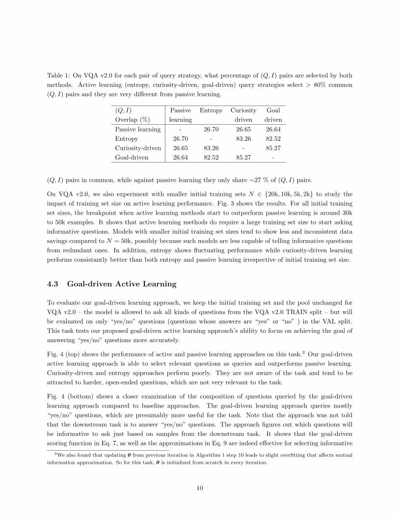
Table 1: On VQA v2.0 for each pair of query strategy, what percentage of (Q, I) pairs are selected by both
methods. Active learning (entropy, curiosity-driven, goal-driven) query strategies select > 80% common
(Q, I) pairs and they are very different from passive learning.
(Q, I) Passive Entropy Curiosity Goal
Overlap (%) learning driven driven
Passive learning - 26.70 26.65 26.64
Entropy 26.70 - 83.26 82.52
Curiosity-driven 26.65 83.26 - 85.27
Goal-driven 26.64 82.52 85.27 -
(Q, I) pairs in common, while against passive learning they only share ∼27 % of (Q, I) pairs.
On VQA v2.0, we also experiment with smaller initial training sets N ∈ {20k, 10k, 5k, 2k} to study the
impact of training set size on active learning performance. Fig. 3 shows the results. For all initial training
set sizes, the breakpoint when active learning methods start to outperform passive learning is around 30k
to 50k examples. It shows that active learning methods do require a large training set size to start asking
informative questions. Models with smaller initial training set sizes tend to show less and inconsistent data
savings compared to N = 50k, possibly because such models are less capable of telling informative questions
from redundant ones. In addition, entropy shows fluctuating performance while curiosity-driven learning
performs consistantly better than both entropy and passive learning irrespective of initial training set size.
4.3 Goal-driven Active Learning
To evaluate our goal-driven learning approach, we keep the initial training set and the pool unchanged for
VQA v2.0 – the model is allowed to ask all kinds of questions from the VQA v2.0 TRAIN split – but will
be evaluated on only “yes/no” questions (questions whose answers are “yes” or “no” ) in the VAL split.
This task tests our proposed goal-driven active learning approach’s ability to focus on achieving the goal of
answering “yes/no” questions more accurately.
Fig. 4 (top) shows the performance of active and passive learning approaches on this task.3 Our goal-driven
active learning approach is able to select relevant questions as queries and outperforms passive learning.
Curiosity-driven and entropy approaches perform poorly. They are not aware of the task and tend to be
attracted to harder, open-ended questions, which are not very relevant to the task.
Fig. 4 (bottom) shows a closer examination of the composition of questions queried by the goal-driven
learning approach compared to baseline approaches. The goal-driven learning approach queries mostly
“yes/no” questions, which are presumably more useful for the task. Note that the approach was not told
that the downstream task is to answer “yes/no” questions. The approach figures out which questions will
be informative to ask just based on samples from the downstream task. It shows that the goal-driven
scoring function in Eq. 7, as well as the approximations in Eq. 9 are indeed effective for selecting informative
3We also found that updating θ from previous iteration in Algorithm 1 step 10 leads to slight overfitting that affects mutual
information approximation. So for this task, θ is initialized from scratch in every iteration.
10

Figure 3: Active learning with N = 20k, 10k, 5k, 2k initial training set size. When dataset size is small,
active learning is unable to outperform passive learning. The breakpoint when active learning methods start
to perform better is around 30k to 50k examples. Best viewed in color.
0.38
0.4
0.42
0.44
0.46
0.48
20000 40000 80000 160000
VQ
A A
ccu
racy
Training Set Size
VQA v2.0 N=20k initial
0.38
0.4
0.42
0.44
0.46
20000 40000 80000 160000
VQ
A A
ccu
racy
Training Set Size
VQA v2.0 N=5k initial
0.38
0.4
0.42
0.44
0.46
20000 40000 80000 160000
VQ
A A
ccu
racy
Training Set Size
VQA v2.0 N=10k initial
Curiosity-driven
Entropy
Passive
0.38
0.4
0.42
0.44
0.46
20000 40000 80000 160000
VQ
A A
ccu
racy
Training Set Size
VQA v2.0 N=2k initial
Curiosity-driven
Entropy
Passive
11

Figure 4: Top: Goal-driven active learning of VQA for answering only “yes/no” questions. Our goal-driven
active learning approach outperforms passive learning and other active learning approaches. Bottom: Query
compositions of active learning approaches, on VQA v2.0 dataset for the task of answering only “yes/no”
questions. Our goal-driven active learning approach queries mostly “yes/no” questions. Best viewed in color.
0.66
0.68
0.7
0.72
50000 150000
VQ
A A
ccu
racy
Training Set Size
VQA v2.0 Test on “Yes/No” Questions
Goal-driven
Passive learning
Curiosity-driven
Entropy
0
0.2
0.4
0.6
0.8
1
0 10 20 30 40 50
“Yes
/No
” Q
ues
tio
n
Iteration
VQA v2.0 Test on “Yes/No” Questions
Query Composition
Goal-driven
Passive learning
Curiosity-driven
Entropy
12

Figure 5: Goal-driven active learning of VQA for answering only “yes/no” questions, compared to passive
learning that “cheats” and queries only “yes/no” questions. Best viewed in color.
0.66
0.68
0.7
0.72
50000 150000
VQ
A A
ccu
racy
Training Set Size
VQA v2.0 Test on “Yes/No” Questions
"Yes/No"
questions only
Goal-driven
questions.
As an “upper bound”, it is reasonable to assume4 that “yes/no” questions are more desirable for this task.
Imagine a passive learning method that “cheats”: one that is aware that it will be tested only on “yes/no”
questions, as well as knowing which questions are “yes/no’ questions in the pool, so it restricts itself to query
only “yes/no” questions. How does our goal-driven learning approach compare with such a method that
only learns from “yes/no” questions? Fig. 5 shows the results. Our goal-driven learning is able to compete
with the “cheating” approach. In fact, of all 167,499 “yes/no” questions in the VQA v2.0 TRAIN split,
goal-driven learning finds 38% of them by iteration 25, and 50% of them by iteration 50. That might also
have made finding the remaining “yes/no” questions more difficult which explains the drop of the rate of
“yes/no” question towards later iterations. We expect that a larger pool (i.e. a larger VQA dataset) would
reduce these issues.
5 Discussion
In this work we discussed three active learning strategies – cramming (entropy), curiosity-driven learning
and goal-driven learning – for Visual Question Answering using deep multimodal neural networks. Our
results show that deep VQA models require 30k - 50k training questions for active learning before they are
able to ask informative questions and achieve better scaling than randomly selecting questions for labeling.
4Note that this is not necessarily the case. Even non-yes/no questions can help a VQA model get better at answering yes/no
questions by learning concepts from non-yes/no questions that can later come handy for yes/no questions. For example “Q:
What is the man doing? A: Surfing” can be as useful as “Q: Is the man surfing? A: Yes”.
13

Once the training set is large enough, several active learning strategies achieve significant savings in answer
annotation cost. Our proposed goal-driven query strategy in particular, shows a significant advantage on
improving performance when the downstream task involves answering a specific type of VQA questions.
Jointly selecting batches of examples as queries [30] and formulating active learning as a decision making
problem [14] (greedily selecting the batch that reduces entropy by the most for the current iteration may
not be the optimal decision) have been shown to improve optimality in active learning query selection.
Combining those approaches with deep neural networks under the Bayesian Neural Network framework are
promising future directions.
The pool-based active learning setup explored in this work selects unlabeled human generated question-
image pairs and asks the oracle for answers. For building VQA datasets however, collecting human-generated
questions paired with each image is also a substantial portion of the overall cost. Hence, starting from a
bank of questions and an unaligned bank of images, and having the model decide which question it would
like to pair with each image to use as a query would result in a further reduction in cost. Note that such
a model would need to not only reason about the informativeness of a question-image pair, but also about
the relevance of a question to the image [27, 22]. Evaluating such an approach would require collecting new
VQA datasets with humans in the loop to give answers – which we show would require 30k - 50k answers
before the model could start selecting informative images and questions. Going one step further, we could
also envision a model that generates new questions rather than selecting from a pool of questions. That
would require a generative model that can perform inference to optimize for the active learning objectives.
We hope that our work serves as a foundation for these future research directions.
Acknowledgements
We thank Michael Cogswell and Qing Sun for discussions about the active learning strategies. This work was
funded in part by an NSF CAREER award, ONR YIP award, Allen Distinguished Investigator award from
the Paul G. Allen Family Foundation, Google Faculty Research Award, and Amazon Academic Research
Award to DP. The views and conclusions contained herein are those of the authors and should not be
interpreted as necessarily representing the official policies or endorsements, either expressed or implied, of
the U.S. Government, or any sponsor.
References
[1] S. Antol, A. Agrawal, J. Lu, M. Mitchell, D. Batra, C. L. Zitnick, and D. Parikh. VQA: Visual Question
Answering. In Proceedings of the IEEE International Conference on Computer Vision (ICCV), pages
2425–2433. IEEE, 2015.
[2] C. Blundell, J. Cornebise, K. Kavukcuoglu, and D. Wierstra. Weight uncertainty in neural network.
In Proceedings of the 32nd International Conference on Machine Learning (ICML), pages 1613–1622.
PMLR, 2015.
14

[3] A. Das, S. Kottur, K. Gupta, A. Singh, D. Yadav, J. M. Moura, D. Parikh, and D. Batra. Visual Dialog.
In Proceedings of the IEEE Conference on Computer Vision and Pattern Recognition (CVPR). IEEE,
2017.
[4] A. Das, S. Kottur, J. M. Moura, S. Lee, and D. Batra. Learning cooperative visual dialog agents with
deep reinforcement learning. arXiv preprint arXiv:1703.06585, 2017.
[5] H. de Vries, F. Strub, S. Chandar, O. Pietquin, H. Larochelle, and A. Courville. GuessWhat?! Visual
object discovery through multi-modal dialogue. In Proceedings of the IEEE Conference on Computer
Vision and Pattern Recognition (CVPR). IEEE, 2017.
[6] Y. Gal and Z. Ghahramani. Dropout as a Bayesian approximation: Representing model uncertainty
in deep learning. In Proceedings of the 33rd International Conference on Machine Learning (ICML),
pages 1050–1059. PMLR, 2016.
[7] Y. Gal, R. Islam, and Z. Ghahramani. Deep Bayesian active learning with image data. In Proceedings
of the 34th International Conference on Machine Learning (ICML), pages 1183–1192. PMLR, 2017.
[8] H. Gao, J. Mao, J. Zhou, Z. Huang, L. Wang, and W. Xu. Are you talking to a machine? Dataset and
methods for multilingual image question. In Proceedings of the 28th Advances in Neural Information
Processing Systems (NIPS), pages 2296–2304, 2015.
[9] D. Geman, S. Geman, N. Hallonquist, and L. Younes. Visual Turing test for computer vision systems.
volume 112, pages 3618–3623. National Academy of Sciences, 2015.
[10] J. Gordon and B. Van Durme. Reporting bias and knowledge acquisition. In Proceedings of the 2013
Workshop on Automated Knowledge Base Construction (AKBC), pages 25–30. ACM, 2013.
[11] Y. Goyal, T. Khot, D. Summers-Stay, D. Batra, and D. Parikh. Making the V in VQA matter: Elevating
the role of image understanding in Visual Question Answering. In Proceedings of the IEEE Conference
on Computer Vision and Pattern Recognition (CVPR). IEEE, 2017.
[12] Y. Guo and R. Greiner. Optimistic active-learning using mutual information. In Proceedings of the 22nd
International Joint Conference on Artificial Intelligence (IJCAI), volume 7, pages 823–829. AAAI, 2007.
[13] N. Houlsby, F. Huszar, Z. Ghahramani, and M. Lengyel. Bayesian active learning for classification and
preference learning. arXiv preprint arXiv:1112.5745, 2011.
[14] S. Javdani, Y. Chen, A. Karbasi, A. Krause, D. Bagnell, and S. S. Srinivasa. Near optimal Bayesian
active learning for decision making. In Proceedings of the 17th International Conference on Artificial
Intelligence and Statistics (AISTATS), pages 430–438. PMLR, 2014.
[15] K. Kafle and C. Kanan. Visual Question Answering: Datasets, algorithms, and future challenges.
Computer Vision and Image Understanding, 2017.
[16] J. Krause, B. Sapp, A. Howard, H. Zhou, A. Toshev, T. Duerig, J. Philbin, and L. Fei-Fei. The
unreasonable effectiveness of noisy data for fine-grained recognition. In Proceedings of the 14th European
Conference on Computer Vision (ECCV), pages 301–320. Springer, 2016.
[17] A. Krishnakumar. Active learning literature survey. Technical Report, University of California, Santa
Cruz, 2007.
[18] T.-Y. Lin, M. Maire, S. Belongie, J. Hays, P. Perona, D. Ramanan, P. Dollar, and C. L. Zitnick.
Microsoft COCO: Common objects in context. In Proceedings of the 13th European Conference on
Computer Vision (ECCV), pages 740–755. Springer, 2014.
15

[19] X. Lin and D. Parikh. Leveraging Visual Question Answering for image-caption ranking. In Proceedings
of the 14th European Conference on Computer Vision (ECCV), pages 261–277. Springer, 2016.
[20] J. Lu, X. Lin, D. Batra, and D. Parikh. Deeper LSTM and normalized CNN Visual Question Answering
model. https://github.com/VT-vision-lab/VQA_LSTM_CNN, 2015.
[21] J. Lu, J. Yang, D. Batra, and D. Parikh. Hierarchical question-image co-attention for visual question
answering. In Proceedings of the 29th Advances in Neural Information Processing Systems (NIPS),
pages 289–297, 2016.
[22] A. Mahendru, V. Prabhu, A. Mohapatra, D. Batra, and S. Lee. The promise of premise: Harnessing
question premises in Visual Question Answering. In Proceedings of the Conference on Empirical Methods
in Natural Language Processing (EMNLP), pages 937–946. ACL, 2017.
[23] M. Malinowski, M. Rohrbach, and M. Fritz. Ask your neurons: A neural-based approach to answering
questions about images. In Proceedings of the IEEE International Conference on Computer Vision
(ICCV), pages 1–9. IEEE, 2015.
[24] D. Mishkin, N. Sergievskiy, and J. Matas. Systematic evaluation of convolution neural network advances
on the ImageNet. Computer Vision and Image Understanding, 161:11–19, 2017.
[25] N. Mostafazadeh, C. Brockett, B. Dolan, M. Galley, J. Gao, G. P. Spithourakis, and L. Vanderwende.
Image-grounded conversations: Multimodal context for natural question and response generation. arXiv
preprint arXiv:1701.08251, 2017.
[26] N. Mostafazadeh, I. Misra, J. Devlin, M. Mitchell, X. He, and L. Vanderwende. Generating natural ques-
tions about an image. In Proceedings of the 54th Annual Meeting of the Association for Computational
Linguistics, volume 1, pages 1802–1813. ACL, 2016.
[27] A. Ray, G. Christie, M. Bansal, D. Batra, and D. Parikh. Question relevance in VQA: Identifying non-
visual and false-premise questions. In Proceedings of the Conference on Empirical Methods in Natural
Language Processing (EMNLP), pages 919–924. ACL, 2016.
[28] M. Ren, R. Kiros, and R. Zemel. Exploring models and data for image question answering. In Proceedings
of the 28th Advances in Neural Information Processing Systems (NIPS), pages 2953–2961, 2015.
[29] N. Roy and A. Mccallum. Toward optimal active learning through Monte Carlo estimation of error
reduction. In Proceedings of the 18th International Conference on Machine Learning (ICML), pages
441–448. Morgan Kaufmann Publishers, 2001.
[30] O. Sener and S. Savarese. A geometric approach to active learning for convolutional neural networks.
arXiv preprint arXiv:1708.00489, 2017.
[31] B. Settles. Active learning literature survey. Computer Science Technical Report (TR1648), University
of Wisconsin, Madison, 2010.
[32] K. Simonyan and A. Zisserman. Very deep convolutional networks for large-scale image recognition.
arXiv preprint arXiv:1409.1556, 2014.
[33] F. Strub, H. de Vries, J. Mary, B. Piot, A. Courville, and O. Pietquin. End-to-end optimization of
goal-driven and visually grounded dialogue systems. In Proceedings of the 26th International Joint
Conference on Artificial Intelligence (IJCAI), pages 2765–2771. AAAI, 2017.
16

[34] S. Zhou, Q. Chen, and X. Wang. Active deep networks for semi-supervised sentiment classification.
In Proceedings of the 23rd International Conference on Computational Linguistics (Coling): Posters,
pages 1515–1523. ACL, 2010.
[35] X. Zhu, J. Lafferty, and Z. Ghahramani. Combining active learning and semi-supervised learning using
gaussian fields and harmonic functions. In ICML 2003 workshop on The Continuum from Labeled to
Unlabeled Data in Machine Learning and Data Mining, pages 58–65, 2003.
17

A Fast Approximation of Goal-driven Scoring Function
In Section 3.2, we discuss our proposed goal-driven query strategy that minimizes uncertainty (entropy) on
answers A′t to a given set of unlabeled test question-image pairs (Q′t, I′t), t = 1, 2, ...T , against which the
model will be evaluated. It queries (Q, I) pairs which maximize:
sgoal(Q, I)
=∑t
H(A′t)−H(A′t|A)
=∑t
I(A;A′t)
=∑t
∑a
∑a′
P (A = a,A′t = a′|Q, I,Q′t, I ′t) logP (A = a,A′t = a′|Q, I,Q′t, I ′t)P (A = a|Q, I)P (A′t = a′|Q′t, I ′t)
(10)
Recall that we propose an approximation for term P (A = a,A′t = a′|Q, I,Q′t, I ′t) as follows:
P (A = a,A′t = a′|Q, I,Q′t, I ′t)
= EωP (A = a|Q, I,ω)P (A′t = a′|Q′t, I ′t,ω)
≈ Eω∼qθ(ω)P (A = a|Q, I,ω)P (A′t = a′|Q′t, I ′t,ω) (11)
Let us define four matrices M1,D1,M2(t),D2(t) as follows:
M1 =
P (A = a1|Q, I,ω1) P (A = a2|Q, I,ω1) . . . P (A = aJ |Q, I,ω1)
P (A = a1|Q, I,ω2) P (A = a2|Q, I,ω2) P (A = aJ |Q, I,ω2)...
. . ....
P (A = a1|Q, I,ωM ) P (A = a2|Q, I,ωM ) . . . P (A = aJ |Q, I,ωM )
(12)
D1 = Diag( [P (A = a1|Q, I) P (A = a2|Q, I) . . . P (A = aJ |Q, I)
] )(13)
M2(t) =
P (A′t = a1|Q′t, I ′t,ω1) P (A′t = a2|Q′t, I ′t,ω1) . . . P (A′t = aJ |Q′t, I ′t,ω1)
P (A′t = a1|Q′t, I ′t,ω2) P (A′t = a2|Q′t, I ′t,ω2) P (A′t = aJ |Q′t, I ′t,ω2)...
. . ....
P (A′t = a1|Q′t, I ′t,ωM ) P (A′t = a2|Q′t, I ′t,ωM ) . . . P (A′t = aJ |Q′t, I ′t,ωM )
(14)
D2(t) = Diag( [P (A′t = a1|Q′t, I ′t) P (A′t = a2|Q′t, I ′t) . . . P (A′t = aJ |Q′t, I ′t)
] )(15)
18

Here M1 is an M ×J matrix, D1 is a J ×J matrix, M2(t) is an M ×J matrix and D2(t) is a J ×J matrix.
With M1,D1,M2(t),D2(t) we could rewrite Eq. 11 in matrix form:
P (A = a1, A
′t = a1|Q, I,Q′t, I ′t) . . . P (A = a1, A
′t = aJ |Q, I,Q′t, I ′t)
.... . .
...
P (A = aJ , A′t = a1|Q, I,Q′t, I ′t) . . . P (A = aJ , A
′t = aJ |Q, I,Q′t, I ′t)
≈ 1
MMT
1 M2(t) (16)
Let Sum(·) be an operator on a matrix that sums up all elements in that matrix. Combining Eq. 10 and
Eq. 16, our goal-driven scoring function can be approximately computed as follows:
sgoal(Q, I)
=∑t
∑a
∑a′
P (A = a,A′t = a′|Q, I,Q′
t, I′t) log
P (A = a,A′t = a′|Q, I,Q′
t, I′t)
P (A = a|Q, I)P (A′t = a′|Q′
t, I′t)
≈∑t
Sum{[ 1
MMT
1 M2(t)]◦ log
[ 1
MD1M
T1 M2(t)D2(t)
]}Rewriting in matrix form.
≈∑t
1
2Sum
{−
1
MMT
1 M2(t) +1
M2
[MT
1 M2(t)]◦[D1M
T1 M2(t)D2(t)
]}x log x ≈
1
2(−x + x2).
=∑t
−1
2+
1
2M2Sum
{[MT
1 M2(t)]◦[D1M
T1 M2(t)D2(t)
]}Sum of P (A,A′
t) reduces to 1.
=∑t
−1
2+
1
2M2Tr{[MT
1 M2(t)][D1M
T1 M2(t)D2(t)
]T}Sum(A ◦B) = Tr(ABT ).
=∑t
−1
2+
1
2M2Tr[MT
1 M2(t)D2(t)MT2 (t)M1D1
]=∑t
−1
2+
1
2M2Tr[M1D1M
T1 M2(t)D2(t)MT
2 (t)]
Property of trace.
=∑t
−1
2+
1
2M2Sum
{[M1D1M
T1
]◦[M2(t)D2(t)MT
2 (t)]}
Tr(ABT ) = Sum(A ◦B).
=∑t
−1
2+
1
2EωEω′
[∑a
P (A = a|Q, I,ω)P (A = a|Q, I,ω′)
P (A = a|Q, I)Rewriting in probability form.
∑a
P (A′t = a|Q′
t, I′t,ω)P (A′
t = a|Q′t, I
′t,ω
′)
P (A′t = a|Q′
t, I′t)
]=
1
2EωEω′
[∑a
P (A = a|Q, I,ω)P (A = a|Q, I,ω′)
P (A = a|Q, I)Rearranging summation.
∑t
∑a
P (A′t = a|Q′
t, I′t,ω)P (A′
t = a|Q′t, I
′t,ω
′)
P (A′t = a|Q′
t, I′t)
]−∑t
1
2(17)
Which is Eq. 9 in Section 3.2.
As stated in Section 3.2, the above equation can be computed as a dot-product between two vectors of
length M2. One vector is matrix 1MM1D1M
T1 expanded into a vector. It only involves pool questions
(Q, I). The other vector is 1M
∑tM2(t)D2(t)MT
2 (t) expanded into a vector. It only involves test questions
(Q′t, I′t) and it is shared for all pool questions (Q, I), so it can be precomputed for all (Q, I). Precomputing
1M
∑tM2(t)D2(t)MT
2 (t) for test questions has a time complexity ofO(TJM2). Note thatD2(t) is a diagonal
19

Figure 6: Convergence of Monte Carlo approximation to entropy, curiosity-driven and goa-driven scoring
functions in terms of rank correlation. We compute scores using Eq. 4 (entropy), 5 (curiosity-driven) and
7 (goal-driven) for 200 random examples from the pool using M ∈ {1, 2, 5, 10, 20, 50, 100, 200, 500} samples
from qθ(ω), and compare them with M = 500 in terms of rank correlation (Spearman’s ρ).
0
0.2
0.4
0.6
0.8
1
1.2
1 10 100 1000
Sp
earm
an’s
ρ
Number of ω samples
Monte Carlo Approximation Quality
Entropy
Curiosity-driven
Goal-driven
matrix, so multiplying D2(t) with MT2 (t) only takes O(JM) operations. In the same way, computing
1MM1D1M
T1 for all (Q, I) has a time complexity of O(UJM2). The time complexity of their dot product
for all (Q, I) is merely O(UM2). So the overall time complexity is O(max(U, T )JM2). The overall time
complexity is linear to both dataset size U and T and the number of possible answers J , so our approach
can easily scale to very large datasets and more VQA answers.
B Quality of Approximations
Our entropy, curiosity-driven and goal-driven scoring functions use 3 types of approximations
(a) Variational distribution qθ(ω) as approximation to model parameter distribution p(ω|Dtrain).
(b) Monte Carlo sampling over qθ(ω) for computing expectation over p(ω|Dtrain).
(c) Fast approximation to mutual information in Eq. 17.
For (a), since the space of model parameters is very large, it is intractable to evaluate how accurate qθ(ω)
substitutes p(ω|Dtrain) for expectation computation. But nevertheless our goal-driven learning results in
Section 4.3 suggest that Eq. 9 computed using qθ(ω) is indeed useful for selecting relevant examples. It
remains as an open problem that how to quantitatively evaluate the quality of qθ(ω) for the purpose of
uncertainty estimation and expectation computation.
20
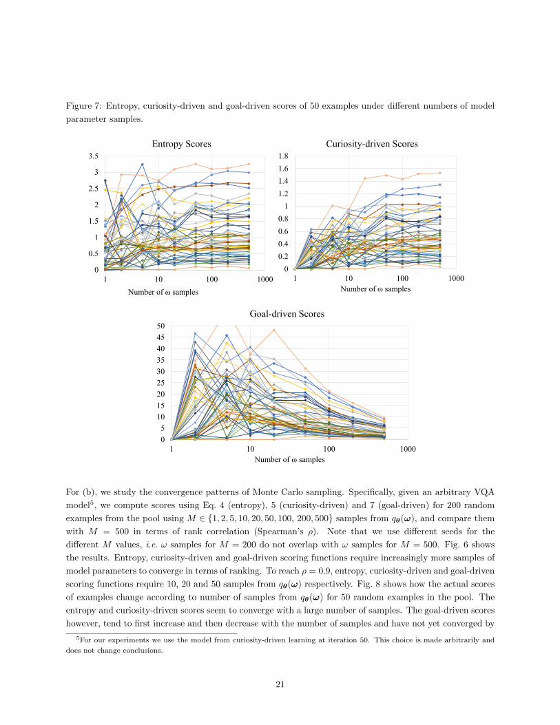
Figure 7: Entropy, curiosity-driven and goal-driven scores of 50 examples under different numbers of model
parameter samples.
0
5
10
15
20
25
30
35
40
45
50
1 10 100 1000
Number of ω samples
Goal-driven Scores
0
0.5
1
1.5
2
2.5
3
3.5
1 10 100 1000
Number of ω samples
Entropy Scores
0
0.2
0.4
0.6
0.8
1
1.2
1.4
1.6
1.8
1 10 100 1000
Number of ω samples
Curiosity-driven Scores
For (b), we study the convergence patterns of Monte Carlo sampling. Specifically, given an arbitrary VQA
model5, we compute scores using Eq. 4 (entropy), 5 (curiosity-driven) and 7 (goal-driven) for 200 random
examples from the pool using M ∈ {1, 2, 5, 10, 20, 50, 100, 200, 500} samples from qθ(ω), and compare them
with M = 500 in terms of rank correlation (Spearman’s ρ). Note that we use different seeds for the
different M values, i.e. ω samples for M = 200 do not overlap with ω samples for M = 500. Fig. 6 shows
the results. Entropy, curiosity-driven and goal-driven scoring functions require increasingly more samples of
model parameters to converge in terms of ranking. To reach ρ = 0.9, entropy, curiosity-driven and goal-driven
scoring functions require 10, 20 and 50 samples from qθ(ω) respectively. Fig. 8 shows how the actual scores
of examples change according to number of samples from qθ(ω) for 50 random examples in the pool. The
entropy and curiosity-driven scores seem to converge with a large number of samples. The goal-driven scores
however, tend to first increase and then decrease with the number of samples and have not yet converged by
5For our experiments we use the model from curiosity-driven learning at iteration 50. This choice is made arbitrarily and
does not change conclusions.
21

M = 500 samples, which is a limitation of the Monte Carlo sampling approach. Despite that, the relative
rankings based on which the queries are selected have mostly converged. Upper- and lower-bounds of Eq. 7
that might improve convergence are opportunities for future research.
For (c), we plot goal-driven scores Eq. 7 as the x-axis versus our fast approximations Eq. 9 as the y-axis for
200 random examples from the pool using M = {2, 5, 10, 20, 50, 100, 200, 500} samples from qθ(ω). Because
Eq. 7 does not scale well to large datasets, we use a subset of 200 random (Q′t, I′t) pairs from the VAL split
as the test domain for both Eq. 7 and Eq. 9. Fig. 8 shows the results. Our fast approximations are mostly
linear to the goal-driven scores. The slope changes according to the number of model parameter samples M .
That is probably because our approximation 12 (−x+ x2) (see Section A for details) overestimates x log x for
x > 1. The rank correlations between goal-driven scores and their fast approximations remain high, e.g.,
above ρ > 0.96 even for M = 500, which is sufficient for query selection.
22

Figure 8: Our fast approximations using Eq. 9 versus the original goal-driven scores computed using Eq. 7
under M = {2, 5, 10, 20, 50, 100, 200, 500} samples of model parameters. Our approximations have high rank
correlation with scores computed using the original method.
0
5
10
15
20
25
30
35
40
45
0 20 40 60
Our
Fas
t A
ppro
xim
atio
n
Goal-driven Scoring Function
𝜌=0.9945
0
10
20
30
40
50
60
70
0 20 40 60 80
Our
Fas
t A
ppro
xim
atio
nGoal-driven Scoring Function
𝜌=0.9898
0
10
20
30
40
50
60
70
0 20 40 60
Our
Fas
t A
ppro
xim
atio
n
Goal-driven Scoring Function
𝜌=0.9860
0
10
20
30
40
50
60
70
80
0 20 40 60
Our
Fas
t A
ppro
xim
atio
n
Goal-driven Scoring Function
𝜌=0.9784
0
10
20
30
40
50
60
70
0 10 20 30 40
Our
Fas
t A
ppro
xim
atio
n
Goal-driven Scoring Function
𝜌=0.9724
0
10
20
30
40
50
60
0 10 20 30
Our
Fas
t A
ppro
xim
atio
n
Goal-driven Scoring Function
𝜌=0.9735
0
5
10
15
20
25
30
35
40
45
0 5 10 15 20
Our
Fas
t A
ppro
xim
atio
n
Goal-driven Scoring Function
𝜌=0.9641
0
5
10
15
20
25
30
35
0 5 10 15
Our
Fas
t A
ppro
xim
atio
n
Goal-driven Scoring Function
𝜌=0.9686
M = 2 M = 5
M = 10 M = 20
M = 50 M = 100
M = 200 M = 500
Fast Approximation to Goal-driven Scoring Function
23