UNITEXT for Physics

Victor Ilisie

Concepts in Quantum Field TheoryA Practitioner's Toolkit

UNITEXT for Physics

Series editors

Michele Cini, Roma, ItalyAttilio Ferrari, Torino, ItalyStefano Forte, Milano, ItalyGuido Montagna, Pavia, ItalyOreste Nicrosini, Pavia, ItalyLuca Peliti, Napoli, ItalyAlberto Rotondi, Pavia, Italy

More information about this series at http://www.springer.com/series/13351

Victor Ilisie

Concepts in QuantumField TheoryA Practitioner’s Toolkit

123

Victor IlisieUniversity of ValenciaValenciaSpain

ISSN 2198-7882 ISSN 2198-7890 (electronic)UNITEXT for PhysicsISBN 978-3-319-22965-2 ISBN 978-3-319-22966-9 (eBook)DOI 10.1007/978-3-319-22966-9

Library of Congress Control Number: 2015946995

Springer Cham Heidelberg New York Dordrecht London© Springer International Publishing Switzerland 2016This work is subject to copyright. All rights are reserved by the Publisher, whether the whole or partof the material is concerned, specifically the rights of translation, reprinting, reuse of illustrations,recitation, broadcasting, reproduction on microfilms or in any other physical way, and transmissionor information storage and retrieval, electronic adaptation, computer software, or by similar or dissimilarmethodology now known or hereafter developed.The use of general descriptive names, registered names, trademarks, service marks, etc. in thispublication does not imply, even in the absence of a specific statement, that such names are exempt fromthe relevant protective laws and regulations and therefore free for general use.The publisher, the authors and the editors are safe to assume that the advice and information in thisbook are believed to be true and accurate at the date of publication. Neither the publisher nor theauthors or the editors give a warranty, express or implied, with respect to the material contained herein orfor any errors or omissions that may have been made.

Printed on acid-free paper

Springer International Publishing AG Switzerland is part of Springer Science+Business Media(www.springer.com)

To my wife and daughter

Preface

This book is intended to be advanced undergraduate–graduate friendly. With a lessstrict yet formal language, it intends to clarify and structure in a very logical mannerconcepts that can be confusing in Quantum Field Theory. It does not replace aformal book on the subject. Its main goal is to be a helpful complementary tool forbeginners and not-so-beginners in this field. The reader is expected to be at leastfamiliar with basic notions of Quantum Field Theory as well as basics of SpecialRelativity. However, most of the times being familiar with Special Relativitydoesn’t mean being familiar with tensor algebra or tensor calculus in general. Manyphysics books assume that the reader is already familiar with tensors, so they begindirectly with advanced topics. On the other hand, many mathematical books aresomewhat too formal for a young physicist. Thus, I have introduced at the begin-ning, a nicely self-contained, student friendly chapter, which introduces the tensorformalism in general, as well as the concept of a manifold. This is done byassuming only that the the reader is familiar with the notions of vectors and vectorspaces. Key aspects of Special Relativity are also covered.

The kinematics needed for the most common relativistic processes is given. It isa logical schematic list of all the relevant and most important formulae needed forcalculating relativistic collisions and decays. It includes one-to-two andone-to-three body decays, and also the two-to-two scattering process both in thecenter of mass and laboratory frames. It also includes simplified general formulae ofone, two, and three-body Lorentz invariant phase space. As a bonus, the three andfour-body kinematics in terms of angular observables is also presented.

Noether’s theorem is mostly treated in the literature in a somewhat heuristicmanner by introducing many ad hoc concepts without too many technical details.I try to fix this problem by stating the most general (Lorentz invariant) form of thetheorem and by applying it to a few simple, yet relevant, examples in QuantumField Theory.

I also try to introduce a simple and robust treatment for dimensional regulari-zation and consistently explain the renormalization procedure step-by-step in atransparent manner at all orders, using the QED Lagrangian, which is in my opinion

vii

the most suitable from an academical point of view. I dedicate thus, one chapter inexplaining the Dyson summation algorithm and try to clarify all possible confusionsthat may arise. Various renormalization schemes are also presented.

Infrared divergences, as well as the ultraviolet ones are also extensively treated.I explicitly calculate a few infrared divergent Green functions and show an explicitexample of cancellation of infrared divergences (step by step) using dimensionalregularization. Other interesting topics are also discussed.

Possible issues and confusion for tadpole renormalization are commented andsome illustrative simple examples are given in Chaps. 7 and 9, where we also treatthe renormalization of the W sector of the Standard Model. With the tools givenhere one should find it straightforward to calculate and renormalize any N-pointGreen function at one-loop level. A very short example of a two-loop calculation isalso given.

Valencia Victor IlisieJuly 2015

viii Preface

Acknowledgments

Many thanks to Prof. A. Pich for sharing his clear vision with me, for having thepatience to answer to all my questions and doubts, and for teaching me all kinds ofsubtleties in Quantum Field Theory and renormalization. (Also, I have borrowedmany of his notations and conventions). Many thanks to Prof. J.A. de Azcárragaand Prof. J.N. Salas and for their wonderful classes on tensors, manifolds,Relativity, group theory, and many other advanced topics in physics that haveinspired the first chapter of this book. Specially many thanks to Prof. J.A. deAzcárraga for many helpful comments on this manuscript. Also many thanks toS. Descotes for introducing me to the realm of angular observables. I would alsolike to thank my colleagues G. Torralba, J.S. Martínez, A. Crespo, and P. Bellidofor our endless talks on physics, tensors, Relativity, and life in general. A lot of themerit is theirs. Last but not least, I would like to thank my family, that has alwaysbeen so supportive and taught me the most important lesson of my life, to nevergive up on my dreams.

This work has been supported in part by the Spanish Government and ERDFfunds from the EU Commission [Grants FPA2011-23778 and CSD2007-00042(Consolider Project CPAN)] and by the Spanish Ministry MINECO through the FPIgrant BES-2012-054676.

ix

Contents

1 Vectors, Tensors, Manifolds and Special Relativity . . . . . . . . . . . . 11.1 Tensor Algebra. . . . . . . . . . . . . . . . . . . . . . . . . . . . . . . . . . 11.2 Tensor Calculus . . . . . . . . . . . . . . . . . . . . . . . . . . . . . . . . . 121.3 Manifolds . . . . . . . . . . . . . . . . . . . . . . . . . . . . . . . . . . . . . 151.4 Comments on Special Relativity . . . . . . . . . . . . . . . . . . . . . . 22Further Reading . . . . . . . . . . . . . . . . . . . . . . . . . . . . . . . . . . . . . . 27

2 Lagrangians, Hamiltonians and Noether’s Theorem . . . . . . . . . . . 292.1 Lagragian Formalism. . . . . . . . . . . . . . . . . . . . . . . . . . . . . . 292.2 Noether’s Theorem . . . . . . . . . . . . . . . . . . . . . . . . . . . . . . . 312.3 Examples . . . . . . . . . . . . . . . . . . . . . . . . . . . . . . . . . . . . . . 322.4 Hamiltonian Formalism . . . . . . . . . . . . . . . . . . . . . . . . . . . . 352.5 Continuous Systems . . . . . . . . . . . . . . . . . . . . . . . . . . . . . . 362.6 Hamiltonian Formalism . . . . . . . . . . . . . . . . . . . . . . . . . . . . 392.7 Noether’s Theorem (The General Formulation) . . . . . . . . . . . . 402.8 Examples . . . . . . . . . . . . . . . . . . . . . . . . . . . . . . . . . . . . . . 43Further Reading . . . . . . . . . . . . . . . . . . . . . . . . . . . . . . . . . . . . . . 46

3 Relativistic Kinematics and Phase Space . . . . . . . . . . . . . . . . . . . 473.1 Conventions and Notations. . . . . . . . . . . . . . . . . . . . . . . . . . 473.2 Process: a ! 1þ 2 . . . . . . . . . . . . . . . . . . . . . . . . . . . . . . . 483.3 Process: a ! 1þ 2þ 3 . . . . . . . . . . . . . . . . . . . . . . . . . . . . 493.4 Process: 1þ 2 ! 3þ 4 . . . . . . . . . . . . . . . . . . . . . . . . . . . . 503.5 Lorentz Invariant Phase Space . . . . . . . . . . . . . . . . . . . . . . . 52Further Reading . . . . . . . . . . . . . . . . . . . . . . . . . . . . . . . . . . . . . . 55

4 Angular Distributions . . . . . . . . . . . . . . . . . . . . . . . . . . . . . . . . . 574.1 Three Body Angular Distributions. . . . . . . . . . . . . . . . . . . . . 574.2 Four Body Angular Distributions . . . . . . . . . . . . . . . . . . . . . 61Further Reading . . . . . . . . . . . . . . . . . . . . . . . . . . . . . . . . . . . . . . 67

xi

5 Dirac Algebra. . . . . . . . . . . . . . . . . . . . . . . . . . . . . . . . . . . . . . . 695.1 Dirac Matrices . . . . . . . . . . . . . . . . . . . . . . . . . . . . . . . . . . 695.2 Dirac Traces. . . . . . . . . . . . . . . . . . . . . . . . . . . . . . . . . . . . 715.3 Spinors and Lorentz Transformations. . . . . . . . . . . . . . . . . . . 725.4 Quantum Electrodynamics . . . . . . . . . . . . . . . . . . . . . . . . . . 74Further Reading . . . . . . . . . . . . . . . . . . . . . . . . . . . . . . . . . . . . . . 83

6 Dimensional Regularization. Ultraviolet and InfraredDivergences . . . . . . . . . . . . . . . . . . . . . . . . . . . . . . . . . . . . . . . . 856.1 Master Integral . . . . . . . . . . . . . . . . . . . . . . . . . . . . . . . . . . 856.2 Useful Results . . . . . . . . . . . . . . . . . . . . . . . . . . . . . . . . . . 876.3 Example: Cancellation of UV Divergences. . . . . . . . . . . . . . . 886.4 Feynman Parametrization . . . . . . . . . . . . . . . . . . . . . . . . . . . 896.5 Example: UV Pole . . . . . . . . . . . . . . . . . . . . . . . . . . . . . . . 916.6 Example: IR Poles . . . . . . . . . . . . . . . . . . . . . . . . . . . . . . . 91Further Reading . . . . . . . . . . . . . . . . . . . . . . . . . . . . . . . . . . . . . . 93

7 QED Renormalization . . . . . . . . . . . . . . . . . . . . . . . . . . . . . . . . . 957.1 QED Lagrangian. . . . . . . . . . . . . . . . . . . . . . . . . . . . . . . . . 957.2 Fermionic Propagator, Mass and Field Renormalization . . . . . . 957.3 Bosonic Propagator and Field Renormalization . . . . . . . . . . . . 977.4 Vertex Correction . . . . . . . . . . . . . . . . . . . . . . . . . . . . . . . . 987.5 Renormalization to All Orders . . . . . . . . . . . . . . . . . . . . . . . 997.6 One-Loop Renormalization Example . . . . . . . . . . . . . . . . . . . 1027.7 Renormalization and Tadpoles . . . . . . . . . . . . . . . . . . . . . . . 109Further Reading . . . . . . . . . . . . . . . . . . . . . . . . . . . . . . . . . . . . . . 111

8 One-Loop Two and Three-Point Functions. . . . . . . . . . . . . . . . . . 1138.1 Two-Point Function . . . . . . . . . . . . . . . . . . . . . . . . . . . . . . 1138.2 IR Divergences and the Two-Point Function . . . . . . . . . . . . . 1178.3 Three-Point Function. . . . . . . . . . . . . . . . . . . . . . . . . . . . . . 1208.4 IR Divergences and the Three-Point Function. . . . . . . . . . . . . 1238.5 Two and Three-Body Phase Space in D Dimensions . . . . . . . . 1278.6 Cancellation of IR Divergences . . . . . . . . . . . . . . . . . . . . . . 1288.7 Introduction to Two-Loops. . . . . . . . . . . . . . . . . . . . . . . . . . 136Further Reading . . . . . . . . . . . . . . . . . . . . . . . . . . . . . . . . . . . . . . 140

9 Massive Spin One and Renormalizable Gauges . . . . . . . . . . . . . . 1419.1 Unitary Gauge . . . . . . . . . . . . . . . . . . . . . . . . . . . . . . . . . . 1419.2 Rn Gauges . . . . . . . . . . . . . . . . . . . . . . . . . . . . . . . . . . . . . 1449.3 Gauge Fixing Lagrangian and Renormalization. . . . . . . . . . . . 147Further Reading . . . . . . . . . . . . . . . . . . . . . . . . . . . . . . . . . . . . . . 155

xii Contents

10 Symmetries and Effective Vertices . . . . . . . . . . . . . . . . . . . . . . . . 15710.1 Higgs Decay to a Pair of Photons . . . . . . . . . . . . . . . . . . . . . 157Further Reading . . . . . . . . . . . . . . . . . . . . . . . . . . . . . . . . . . . . . . 161

11 Effective Field Theory. . . . . . . . . . . . . . . . . . . . . . . . . . . . . . . . . 16311.1 Effective Lagrangian . . . . . . . . . . . . . . . . . . . . . . . . . . . . . . 16311.2 Renormalization Group Equations . . . . . . . . . . . . . . . . . . . . . 16411.3 Matching . . . . . . . . . . . . . . . . . . . . . . . . . . . . . . . . . . . . . . 167Further Reading . . . . . . . . . . . . . . . . . . . . . . . . . . . . . . . . . . . . . . 172

12 Optical Theorem. . . . . . . . . . . . . . . . . . . . . . . . . . . . . . . . . . . . . 17312.1 Optical Theorem Deduction . . . . . . . . . . . . . . . . . . . . . . . . . 17312.2 One-Loop Example . . . . . . . . . . . . . . . . . . . . . . . . . . . . . . . 176Further Reading . . . . . . . . . . . . . . . . . . . . . . . . . . . . . . . . . . . . . . 178

Appendix A: Master Integral . . . . . . . . . . . . . . . . . . . . . . . . . . . . . . . 179

Appendix B: Renormalization Group Equations . . . . . . . . . . . . . . . . . 183

Appendix C: Feynman Rules for Derivative Couplings . . . . . . . . . . . . 189

Contents xiii

Chapter 1Vectors, Tensors, Manifolds and SpecialRelativity

Abstract Assuming that the reader is familiar with the notion of vectors, within afew pages, with a few examples, the reader will get to be familiar with the genericpicture of tensors. With the specific notions given in this chapter, the reader willbe able to understand more advanced tensor courses with no further effort. Thetransition between tensor algebra and tensor calculus is done naturally with a veryfamiliar example. The notion of manifold and a few basic key aspects on SpecialRelativity are also presented.

1.1 Tensor Algebra

Beforewe get to define the notion of a tensor, whichwill arise naturally, it is importantto start from the very beginning and remember a fewbasic notions about vector spacesand linear maps (applications) defined over vector spaces. We shall assume that thereader is at least familiar with vectors and vector spaces, so we shall try not to getinto unnecessary details. Let’s, thus, start by considering a vector space Vn of finitedimension n defined over the set of real numbers1 R. Given an arbitrary basis {ei }n

i=1we can write a vector v ∈ Vn as

v = vi ei . (1.1)

One is probably used to see a vector written in the following form

v =∑n

i=1vi ei . (1.2)

Here we will suppress the bold vector symbol and adopt the standard Einstein sum-mation convention for repeated indices, so what we get is the compact form (1.1).Let’s consider an invertible change of basis given by the matrix A (det(A) �= 0). Wecan relate the new basis with the original one by

1In general it could be defined over C, but here, we are not interested in this case. Once the reader isfamiliarized with the notions presented here, it is easy to further study the generalization to complexspaces.

© Springer International Publishing Switzerland 2016V. Ilisie, Concepts in Quantum Field Theory,UNITEXT for Physics, DOI 10.1007/978-3-319-22966-9_1

1

2 1 Vectors, Tensors, Manifolds and Special Relativity

e′j = Ai

j ei , (1.3)

where the upper index of A stands for the row and the lower one for the column(remember that, if not stated otherwise, summation is always performedover repeatedindices). Equivalently one can write the inverse relation

e j = (A−1)ij e′

i . (1.4)

Because v is an invariant quantity, it is straightforward to obtain the transformationlaw for the vector components

v = v j e j = v j (A−1)ij e′

i = v′i e′i . (1.5)

Thus, under an invertible change of basis (1.3) the vector components transform as

v′i = (A−1)ij v

j , (1.6)

or equivalently vi = Aij v

′ j .

1.1.1 Dual Space

The dual space of Vn , denoted as V ∗n is defined as the space of all the linear maps

(applications) from Vn to R:

β : Vn → R

β : v �→ β(v), (1.7)

with the following property

β(λ1u1 + λ2u2) = λ1β(u1) + λ2β(u2), (1.8)

∀ u1, u2 ∈ Vn and ∀ λ1,λ2 ∈ R. The space V ∗n is also a vector space of dimension

n and its elements are usually called covectors. Using an arbitrary basis {ωi }ni=1 an

element β ∈ V ∗n can be written as

β = βi ωi . (1.9)

Therefore, given an element v ∈ Vn the linear map β(v) ∈ R can be explicitly writ-ten as

β(v) = βi ωi (v j e j ) = βi v

j ωi (e j ). (1.10)

1.1 Tensor Algebra 3

In general, the quantity ωi (e j ) depends on the chosen bases {ωi } and {ei }. However,there is one basis of V ∗

n called dual basis of Vn , that has the following simple property

ωi (e j ) = δij , (1.11)

where δij is the Kronecker-delta defined the usual way (δi

j = 0 if i �= j and δij = 1

if i = j). We shall work from now on using the dual basis and instead of writing itselements {ω j } we shall write them {e j }. Thus using this new notation (1.11) turnsinto

ei (e j ) = δij , (1.12)

and so β(v) takes the simple form

β(v) = βi ei (v j e j ) = βi vj ei (e j ) = βi v

j δij = βi v

i . (1.13)

Let’s now deduce how the elements {ei } must transform under a change of the basis{e j } → {e′

j } in order to maintain the duality condition:

ei (e j ) = δij = e′i (e′

j ). (1.14)

Let’s suppose that the transformation {ei } → {e′i } is given by an invertible matrixB (det(B) �= 0):

e′i = Bil el . (1.15)

Inserting (1.3) and (1.15) into (1.14) we easily get

e′i (e′j ) = Bi

l el(Akj ek) = Bi

l Akj el(ek) = Bi

l Akj δ

lk = δi

j . (1.16)

Therefore, we obtain the following relation between the matrices A and B

Bik Ak

j = δij ⇒ B A = I ⇒ A = B−1. (1.17)

where I is the n × n identity matrix. In conclusion, the components of the covectorand the basis of V ∗

n obey the following transformation rules

β′i = A j

i β j , e′i = (A−1)ij e j . (1.18)

4 1 Vectors, Tensors, Manifolds and Special Relativity

1.1.2 Covariant and Contravariant Laws of Transformation

Summing up, given v ∈ Vn a vector (v = vi ei ) and β ∈ V ∗n a covector (β = βi ei ),

we have the following law of transformation for {ei } and {βi }

e′i = A j

i e j , β′i = A j

i β j . (1.19)

We shall call this, the covariant law of transformation. For {ei } and {vi } we havefound

e′i = (A−1)ij e j , v′i = (A−1)i

j vj . (1.20)

We shall call this, the contravariant law of transformation. This is the reasonwhyweuse upper and lower indices, to be able to make the difference between covariant andcontravariant quantities. However, we have to be careful because not every elementwith an upper or a lower index is a covariant or contravariant quantity. We shallsee an explicit example within a few sections.

1.1.3 Theorem

For a finite dimensional vector space Vn , the dual space of its dual space V ∗n , (called

double dual space, denoted as V ∗∗n ) is isomorphic to Vn .

This is just general algebra and we shall not be concerned about giving the proofhere. The important thing that we need to learn from this theorem is that there is aone-to-one correspondence between Vn and V ∗∗

n , thus, in what we are concerned,we learn nothing new from V ∗∗

n . As a consequence, we can safely identify the vectorspace Vn with its double dual V ∗∗

n . Because of this, Vn can be viewed as the spaceof all linear maps from V ∗

n to R, v : V ∗n → R. Therefore, if one identifies Vn with

the dual space of V ∗n then one can make the following definition

e j (ei ) ≡ ei (e j ) = δi

j . (1.21)

Given this definition one can also make another one that will turn out to be useful

v(β) ≡ β(v) = βi vi . (1.22)

After this short reminder, we are now in position to define a more general elementof algebra that generalizes vectors, covectors and linear maps. We are talking ofcourse, about tensors. First we will need to introduce the tensor product.

1.1 Tensor Algebra 5

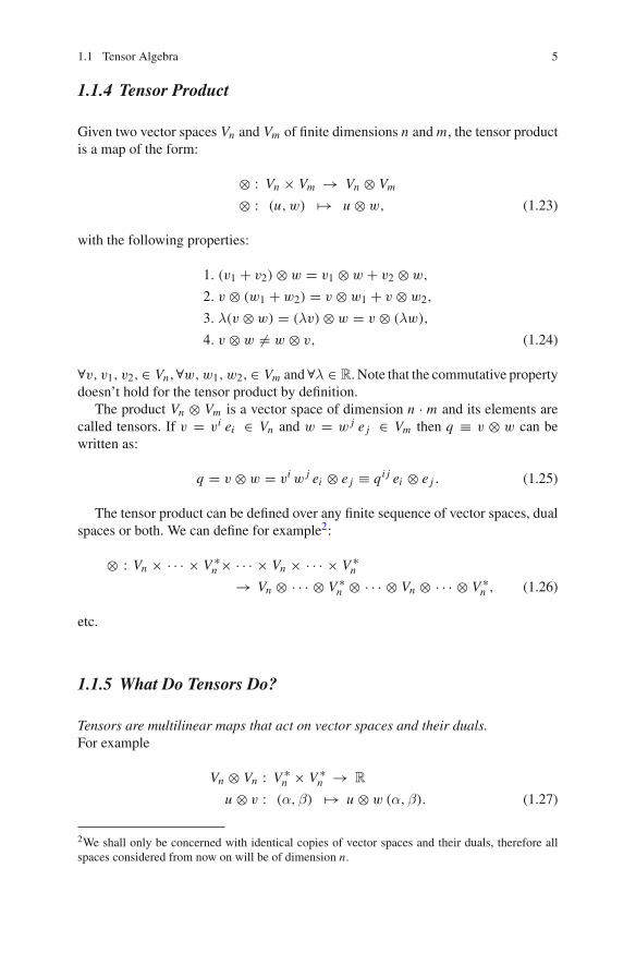
1.1.4 Tensor Product

Given two vector spaces Vn and Vm of finite dimensions n and m, the tensor productis a map of the form:

⊗ : Vn × Vm → Vn ⊗ Vm

⊗ : (u, w) �→ u ⊗ w, (1.23)

with the following properties:

1. (v1 + v2) ⊗ w = v1 ⊗ w + v2 ⊗ w,

2. v ⊗ (w1 + w2) = v ⊗ w1 + v ⊗ w2,

3. λ(v ⊗ w) = (λv) ⊗ w = v ⊗ (λw),

4. v ⊗ w �= w ⊗ v, (1.24)

∀v, v1, v2,∈ Vn , ∀w,w1, w2,∈ Vm and ∀λ ∈ R. Note that the commutative propertydoesn’t hold for the tensor product by definition.

The product Vn ⊗ Vm is a vector space of dimension n · m and its elements arecalled tensors. If v = vi ei ∈ Vn and w = w j e j ∈ Vm then q ≡ v ⊗ w can bewritten as:

q = v ⊗ w = vi w j ei ⊗ e j ≡ qi j ei ⊗ e j . (1.25)

The tensor product can be defined over any finite sequence of vector spaces, dualspaces or both. We can define for example2:

⊗ : Vn × · · · × V ∗n × · · · × Vn × · · · × V ∗

n

→ Vn ⊗ · · · ⊗ V ∗n ⊗ · · · ⊗ Vn ⊗ · · · ⊗ V ∗

n , (1.26)

etc.

1.1.5 What Do Tensors Do?

Tensors are multilinear maps that act on vector spaces and their duals.For example

Vn ⊗ Vn : V ∗n × V ∗

n → R

u ⊗ v : (α,β) �→ u ⊗ w (α,β). (1.27)

2We shall only be concerned with identical copies of vector spaces and their duals, therefore allspaces considered from now on will be of dimension n.

6 1 Vectors, Tensors, Manifolds and Special Relativity

The quantity u ⊗ w (α,β) can be expressed using dual bases as

u ⊗ w (α,β) = u(α) v(β)

= ui ei (α j e j ) vk ek (βl el)

= ui α j ei (ej ) vk βl ek(e

l)

= ui α j δji vk βl δ

lk

= ui αi vk βk (1.28)

However, not all tensors defined over V ∗n × V ∗

n are of the form u ⊗ v. The generalway of defining a tensor will be given in the following sections.

1.1.6 Rank Two Contravariant Tensor

A rank two contravariant tensor, or a (2, 0) tensor is a linear map of the form:

t : V ∗n × V ∗

n → R

t : (α,β) �→ t (α,β), (1.29)

with the following properties:

1. t (λ1α1 + λ2α2, β) = λ1 t (α1, β) + λ2 t (α2, β)

2. t (α, λ1β1 + λ2β2) = λ1 t (α, β1) + λ2 t (α, β2), (1.30)

∀ α,β,α1,α2,β1,β2,∈ V ∗n and ∀ λ1,λ2 ∈ R. It is straightforward to deduce that

the following property also holds

t (λ1α, λ2β) = λ1λ2 t (α,β), (1.31)

∀ α,β ∈ V ∗n and ∀ λ1,λ2 ∈ R. Given α,β ∈ V ∗

n we can write t (α,β) as

t (α,β) = t (αi ei ,β j e

j ) = αi β j t (ei , e j ) ≡ αi β j t i j , (1.32)

where we have defined t (ei , e j ) ≡ t i j as the tensor components related to the givenbasis. Thus, we can express t using a basis and the tensor product as follows

t = t i j ei ⊗ e j , (1.33)

1.1 Tensor Algebra 7

so that,

t (α,β) = t i j ei ⊗ e j (αk ek,βl el)

= t i j αk βl ei ⊗ e j (ek, el)

= t i j αk βl ei (ek)e j (e

l)

= t i j αk βl δki δl

j

= t i j αi β j (1.34)

Whenever t can be separated as t i j = vi w j with u, w ∈ Vn (meaning thatt = v ⊗ w, as in the previous section) it is said that t is a separable tensor.

1.1.7 Rank Two Covariant Tensor

A rank two covariant tensor, or a (0, 2) tensor, is a linear map of the form:

t : Vn × Vn → R

t : (u, v) �→ t (u, v), (1.35)

with the same properties 1, 2 as in the previous case. Thus, we can express t using abasis as follows

t = ti j ei ⊗ e j . (1.36)

Therefore, given u, v ∈ Vn

t (u, v) = ti j ei ⊗ e j (uk ek, vl el)

= ti j uk vl ei ⊗ e j (ek, el)

= ti j uk vl ei (ek)e j (el)

= ti j uk vl δik δ

jl

= ti j ui v j (1.37)

1.1.8 (1, 1) Mixed Tensor

We have to be somewhat careful when we defining mixed tensors. For example, wecan define a (1,1) mixed tensor in two different ways. The first one

8 1 Vectors, Tensors, Manifolds and Special Relativity

t : V ∗n × Vn → R

t : (α, v) �→ t (α, v), (1.38)

with t first acting on V ∗n and afterwards on Vn . It must be written as

t = t ij ei ⊗ e j . (1.39)

The other way of defining a (1,1) tensor is

t : Vn × V ∗n → R

t : (v,α) �→ t (v,α). (1.40)

In this case t must be written as

t = t ji ei ⊗ e j . (1.41)

In order to avoid this confusion one usually leaves blank spaces in between the tensorindices, as it is done here, to indicate the order in which the application acts. Let’stake one last example. Consider the map

t : Vn × V ∗n × V ∗

n × Vn → R. (1.42)

Obviously t must be written as

t = t jki l ei ⊗ e j ⊗ ek ⊗ el . (1.43)

It must be noted that if, for practical calculations, this order does not count, oneusually forgets about the blank spaces. This is pretty usual in many calculations inphysics, for example you will probably find the previous tensor components writtenas t jk

il .

1.1.9 Tensor Transformation Under a Change of Basis

Let’s consider a (2, 0) tensor. Under a change of basis of the form (1.3) we have thefollowing

t = tkl ek ⊗ el = tkl e′i ⊗ e′

j (A−1)ik (A−1)

jl = t ′i j e′

i ⊗ e′j . (1.44)

Thus, the law of transformation of a rank two contravariant tensor is:

t ′i j = tkl (A−1)ik (A−1)

jl (1.45)

1.1 Tensor Algebra 9

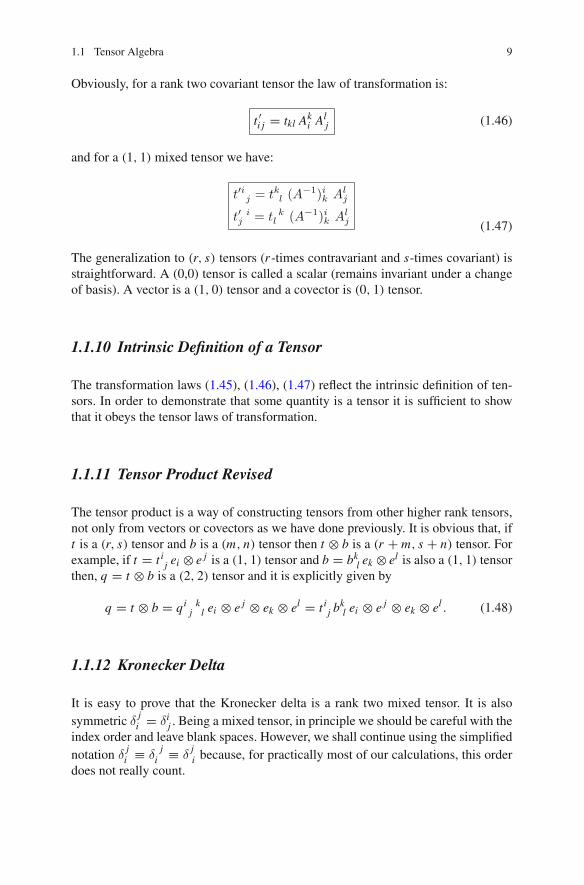
Obviously, for a rank two covariant tensor the law of transformation is:

t ′i j = tkl Aki Al

j (1.46)

and for a (1, 1) mixed tensor we have:

t′ij = tkl (A−1)ik Al

j

t′ ij = t k

l (A−1)ik Alj (1.47)

The generalization to (r, s) tensors (r -times contravariant and s-times covariant) isstraightforward. A (0,0) tensor is called a scalar (remains invariant under a changeof basis). A vector is a (1, 0) tensor and a covector is (0, 1) tensor.

1.1.10 Intrinsic Definition of a Tensor

The transformation laws (1.45), (1.46), (1.47) reflect the intrinsic definition of ten-sors. In order to demonstrate that some quantity is a tensor it is sufficient to showthat it obeys the tensor laws of transformation.

1.1.11 Tensor Product Revised

The tensor product is a way of constructing tensors from other higher rank tensors,not only from vectors or covectors as we have done previously. It is obvious that, ift is a (r, s) tensor and b is a (m, n) tensor then t ⊗ b is a (r + m, s + n) tensor. Forexample, if t = t i

j ei ⊗ e j is a (1, 1) tensor and b = bkl ek ⊗ el is also a (1, 1) tensor

then, q = t ⊗ b is a (2, 2) tensor and it is explicitly given by

q = t ⊗ b = qi kj l ei ⊗ e j ⊗ ek ⊗ el = t i

j bkl ei ⊗ e j ⊗ ek ⊗ el . (1.48)

1.1.12 Kronecker Delta

It is easy to prove that the Kronecker delta is a rank two mixed tensor. It is alsosymmetric δ

ji = δi

j . Being a mixed tensor, in principle we should be careful with theindex order and leave blank spaces. However, we shall continue using the simplifiednotation δ

ji ≡ δ

ji ≡ δ

ji because, for practically most of our calculations, this order

does not really count.

10 1 Vectors, Tensors, Manifolds and Special Relativity

1.1.13 Tensor Contraction

Given a rank (r, s) tensor, we can construct a rank (r − 1, s − 1) rank tensor by con-tracting (summing over) any upper (contravariant) index with any lower (covariant)index. For example, given a rank (2, 2) tensor with components T lk

i j , the quantities

T ′ kj ≡ T ik

i j are the components of a rank (1, 1) tensor.Similarly, one can construct tensors by contracting any upper index of a tensorwith

any lower index of another tensor. Given a rank (1, 2) tensor with components T ijl

and a rank (3, 0) tensor with components K kmn , the quantities Pi mnj ≡ T i

jl K lmn

are the components of a (3, 1) tensor.

1.1.14 Metric Tensor

Given a vector space Vn , we define a metric tensor (rank two covariant) as:

g : Vn × Vn → R

g : (u, v) �→ g(u, v) (1.49)

with the following properties:

1.symmetric gi j = g j i

2.non-singular det(g) �= 0 (1.50)

Of course, we can define the inverse metric tensor (rank two contravariant)

g−1 : V ∗n × V ∗

n → R

g−1 : (m, n) �→ g−1(m, n) (1.51)

with the same two properties as the metric tensor. Thus, g g−1 = I , which can bewritten using the Kronecker delta as

gi j gjk = δk

i . (1.52)

Again, I stands for n × n the identity matrix.

1.1.15 Lowering and Raising Indices

There is a natural way of going from a vector space to its dual by using the metrictensor. Given a vector v = v j e j we can define the covector v∗ = v j e j with

1.1 Tensor Algebra 11

v j = gi jvi , and given a covector β = βi ei we can define a vector β∗ = βi ei with

βi = gi jβ j . This can be generalized for any (r, s) type tensor, and we can use themetric tensor to lower or raise as many tensor indices as we want, for example

R ki j = Rmnk gmi gnj . (1.53)

1.1.16 Scalar Product

Given a metric tensor we can define two important invariant quantities (scalars).First, given two vectors u, v we define their scalar product as:

(u · v) = (v · u) ≡ vi ui = gi j ui v j = gi j ui v j = δij ui v

j . (1.54)

Second, when u = v can define the squared modulus of the vector v ∈ Vn as

v2 ≡ vi vi = gi j vi v j = gi j vi v j = δi

j vi vj . (1.55)

1.1.17 Euclidean Metric

Even though we do not write it down explicitly when working in the usual Euclidean3D space R3, we use the Euclidean metric given by

g = g−1 =⎡

⎣1 0 00 1 00 0 1

⎤

⎦ (1.56)

(for the canonical basis and Cartesian coordinates). The short-hand notation for thisis gi j = gi j = diag{1, 1, 1}.

Invariant Euclidean Length: given two points in space A and B with coordinatesgiven by x and y in a certain reference frame O, we define w ≡ x − y. The squareddistance between these to points in 3D Euclidean space is defined as

w2 ≡ |w|2 = (w1)2 + (w2)2 + (w3)2 = gi j wi w j . (1.57)

We can observe that the length we have just defined is basis independent (obviouslythis has to hold because the distance between two objects doesn’t depend on thereference system, at least from a classical point of view).

12 1 Vectors, Tensors, Manifolds and Special Relativity

As we have already mentioned before, not everything that has an index is atensor. For example, theposition vectors x and y that we are so used to call vectorsmust strictly be called coordinates, because they do not behave as vectors. If wemake a translation from O to another reference frame O ′ so that:

x ′i = xi + ai , y′i = yi + ai , (1.58)

it is clear that

|x ′|2 ≡ (x ′1)2 + (x ′2)2 + (x ′3)2 �= |x|2 ≡ (x1)2 + (x2)2 + (x3)2, (1.59)

and same for |y ′|2. A properly defined vector is w; under the transformation (1.58),w′i = wi so |w ′|2 = |w|2. This simple example (that can be easily generalized toany n-dimensional Euclidean space with any metric) will turn out to be very usefulfor the transition from tensor algebra to tensor calculus.

1.1.18 Vn, En and Rn

In the previous example we have mentioned points in space, without giving anyproper explanation. We shall not give it yet. Within a few sections we shall seethat these points are related to the concept of mani f old. Let us define En as then-dimensional Euclidean space (or manifold) as the abstract set formed by the pointsin space A, B…, with coordinates given by sub-sets of Rn . Even if there is a globalone-to-one relation between the coordinates and the points (between En andRn), wemust not identify the points of the space (nor the space) with the coordinates.Therefore, we will say that

w ∈ Vn ; x, y ∈ Rn ; A, B ∈ En . (1.60)

We shall see in a few sections why it is so important (crucial) to define these threedifferent spaces.

1.2 Tensor Calculus

1.2.1 Tensor Fields

Whenever a vector is defined for every point in space A ∈ En , thus when it is acontinuous function of some parameters xi ∈ R

n , it is called a vector field. How doesit transform? (Obviously now the transformation matrix depends on the parametersxi ). In order to find the natural answer to this question let us take the following

1.2 Tensor Calculus 13

example. Consider again two points A, B ∈ En with coordinates xi , yi in somereference frame and x ′i , y′i in another one (related to the original one by a translationfor example) (with xi , xi , x ′i , x ′i ∈ R

n). Now let’s define Δxi ≡ xi − yi andΔx ′i ≡ x ′i − y′i . We have seen that the following interval is invariant:

Δs2 = gi j Δxi Δx j = Δs′2 = g′i j Δx ′i Δx ′ j . (1.61)

Taking xi and yi to be infinitesimally close (thus x ′i and y′i ) our scalar intervalbecomes differential

ds2 = gi j dxi dx j = ds′2 = g′i j dx ′i dx ′ j . (1.62)

From the previous expression it is natural to identify dxi with the components of avector field. So, under a change of coordinates xi → x ′i , the transformation law forthe components of the vector field is given by the chain rule

dx ′i = ∂x ′i

∂x jdx j , (1.63)

whichwe identify as our contravariant law of transformation. This can be generalizedto any tensor. If a tensor is a continuous function of some parameters xi ∈ R

n , then itis called a tensor field. Taking the usual two examples, (2, 0) and (0, 2) tensor fieldscan be written in the following form3:

t = t i j (x) ei (x) ⊗ e j (x),

l = li j (x) ei (x) ⊗ e j (x). (1.64)

Note that, necessarily the bases also depend on the same parameters xi : for a point Awith coordinates xi

A in a reference frame, and x ′iA in another, a tensor field evaluated

in A denoted as tA, must have a unique value which is independent of the referenceframe. For example for a (2,0) tensor field we have

tA = t i j (xA) ei (xA) ⊗ e j (xA) = t ′i j (x ′A) e′

i (x ′A) ⊗ e′

j (x ′A). (1.65)

A very familiar example where the components ei of the basis depend on the coor-dinates x j are vectors expressed in curvilinear coordinates. The basis is given by

e1(x) ≡ uφ , e2(x) ≡ uθ , e3(x) ≡ ur . (1.66)

with x j = (r, θ,φ).In conclusion, taking quick look at (1.62) and (1.63), we identify the contravari-

ant law of transformation with

3Here we will use the short-hand notation f (xi ) ≡ f (x).

14 1 Vectors, Tensors, Manifolds and Special Relativity

e′i(x′) =∂x′i

∂xlel(x)

t′ij(x′) =∂x′i

∂xl

∂x′j

∂xktlk(x)

... (1.67)

Thus, the covariant law of transformation will be given by

e′i (x ′) = ∂xl

∂x ′i el(x)

t ′i j (x ′) = ∂xl

∂x ′i∂xk

∂x ′ jtlk(x)

. . . (1.68)

The law of transformation for mixed tensor fields is obviously given by

t ′ij (x) = ∂x ′i

∂xl

∂xk

∂x ′ jt l

k(x)

t ′ ij (x) = ∂x ′i

∂xl

∂xk

∂x ′ jt lk (x)

. . . (1.69)

The generalization to (r, s) tensor fields is straightforward. A (0, 0) field is called ascalar field and it obeys:

φ(x) = φ′(x ′) . (1.70)

The expressions (1.67–1.70) represent the intrinsic definition of tensor fields and thisis what you would normally find in many physics books. However, I believe that, inorder to obtain a complete vision and a deeper understanding of tensors, one has togo through all the previous steps.

1.2.2 Tensor Density

Using the the intrinsic definition of tensor fields it is straightforward to introduceanother object which is called tensor density. We say that t i1...ir

j1... js(x) are the

components of a (r, s) tensor density of weight W if under a change of coordinatesxi → x ′i they obey the following transformation law

1.2 Tensor Calculus 15

t ′i1...ir j1... js (x ′) =[det

(∂xi

∂x ′ j

)]W∂x ′i1

∂xl1. . .

∂x ′ir

∂xlr

× ∂xm1

∂x ′ j1. . .

∂xms

∂x ′ jst l1...lr

m1...ms(x) (1.71)

where det(∂xi/∂x ′ j) is the determinant of the Jacobian matrix of the given transfor-

mation. Same definition is valid for any (r, s) type tensor i.e., t i1...il il+1...irj1... jk jk+1... js

(x),etc. One can prove that the totally antisymmetric Levi-Civita symbol

εi1...ik ...im ...in = (−1)p εi1...im ...ik ...in , (1.72)

where p stands for the parity of the permutation (p = 1 for an odd and p = 2 for aneven permutation) is a tensor density of weight W = −1.

We will now move on to the next section and generalize everything to non-Euclidean spaces and introduce properly the concept of manifold.

1.3 Manifolds

We have defined the Euclidean space (manifold) En as the set of points that haveglobal a one-to-one correspondence with R

n . What is, however, the generic defin-ition of a manifold and what happens if the manifold is not Euclidean? Hobson’swonderfully intuitive definition4 is:In general, a manifold is any set that can be continuously parametrized. The numberof independent parameters required to specify any point in the set uniquely is thedimension of the manifold. [. . .] In its most primitive form a general manifold issimply an amorphous collection of points. Most manifolds used in physics, however,are “differential manifolds”, which are continuous and differentiable in the followingway. A manifold is continuous if, in the neighborhood of any point P, there areother points whose coordinates differ infinitesimally from those of P. A manifold isdifferentiable if it is possible to define a scalar field at each point of the manifoldthat can be differentiated anywhere. [. . .] An N-dimensional manifold M of pointsis one for which N independent real coordinates {xi }N

i=1 are required to specify anypoint completely.

For a generic manifold, one can only find small (local) mappings between themanifold andRn . A very familiar example is a surface; in order do describe a surfaceone needs two parameters, therefore we say that a surface is a two-dimensionalmanifold. Let’s now imagine that our surface is flat. If this is the case we can finda global one-to-one mapping between the surface and R

2. However, if we considera sphere, in general one can never find a global mapping between this surface and

4M.P.Hobson,G.P. Efstathiou andA.N.Lanseby,GeneralRelativity,An Introduction for Physicists..

16 1 Vectors, Tensors, Manifolds and Special Relativity

R2 that is able to cover the whole sphere. We can only locally describe parts of the

surface using local charts (regions) of R2. This example can easily be generalizedto any manifold.An N-dimensional differential manifold M is a set of elements (points) P, togetherwith a collection of subsets {Oα} of M that satisfy the following three conditions:

1. ∀ P ∈ M there is at least a subset Oα, so that P ∈ Oα. Equivalently:

M =⋃

α

Oα

2. For each Oα there is a diffeomorphism (differential with its inverse also differen-tial) Ψα:

Ψα : Oα → Ψα(Oα) ≡ Uα ⊆ Rn

M

OαΨα

p

Ψα(p)

Rn

Uα = Ψα(Oα)

3. If Oα ∩ Oβ �= {Ø} then Ψα(Oα ∩ Oβ) and Ψβ(Oα ∩ Oβ) are open sets of Rn andthe application:

Ψβ ◦ Ψ −1α : Ψα(Oα ∩ Oβ) → Ψβ(Oα ∩ Oβ)

is a diffeomorphism. Here we have defined the composed operator Ψβ ◦ Ψ −1α (X) ≡

Ψβ(Ψ −1α (X)). This application is called a change of coordinates.

M

Oβ

Ψβ

Rn

Uβ

OαOα

OβΨα

Rn

Uα

Ψβ ◦ Ψ−1α

The sets (Ψα, Oα) are called charts. The set formed of all charts is called an atlas.Thus, for a given manifoldM of dimension n, if we can find an atlas that contains

only one chart, then we shall say that themanifold is flat or that it has trivial topology.

1.3 Manifolds 17

Going back to the surface example, a surface has two types of curvatures, an intrinsic(Gauss curvature) and an extrinsic one. A surface that has no intrinsic curvature canbe unfolded into a flat surface (for example a cylinder). On the other hand, a sphere isimpossible to unfold into a flat surface (therefore we say it has an intrinsic curvature,or its topology is non trivial).

1.3.1 Embedding

Following these definitions, a curve is a one-dimensionalmanifold, a surface is a two-dimensional one and a solid volume is a three-dimensional one. All these examplesare very familiar. Let’s take for example the curve.We need one parameter to describeit, say t . We can describe this curve in R3 as:

r(t) ≡ (x(t), y(t), z(t)). (1.73)

If we have a surface, as we have mentioned before, we need two parameters todescribe it, say u and v. In R3 we can describe a surface as:

s(u, v) ≡ (x(u, v), y(u, v), z(u, v)), (1.74)

for example,we candescribe regions of the given surface as s(u, v) ≡ (u, v, f (u, v)).In the previous examples we have described (and visualised) these objects in

R3 space. The technical word for describing (or visualising) these objects in R

3 isembedding. We say that we canmake and embedding of curves, surfaces or volumesinR3. However, not all one, two and three-dimensional manifolds are curves surfacesor solid volumes aswe know them.There are for example, two dimensionalmanifoldsthat can not be embedded in R

3 but in a higher dimensional space Rn with n > 3.Thus, these objects are not usual surfaces.

What happens if the manifold we are trying to describe has more than threedimensions? In General Relativity our manifold is formed by space-time points thatwe call events, it is four-dimensional and in general its topology is not trivial. As wehave no information about the existence of any higher dimensional space inwhich ourspace-time can be embedded, our only solution is to abandon the embedding conceptand describe our manifold intrinsically. In order to understand this we shall discussthe classical example. Let’s imagine a civilization that lives in a two dimensionalworld which is a surface. The habitants of this surface can only measure the intrinsiccurvature. Information about the extrinsic curvature is only accessible to an observerthat lives in all tree dimensions. Similarly, we are the civilization that is living infour-dimensional space-time (which is our hyper-surface) and we have no accessto a higher dimensional space (we don’t even know if it exists). We can only makeintrinsic measurements of the curvature of our manifold, which is related to thegravitational force.

18 1 Vectors, Tensors, Manifolds and Special Relativity

1.3.2 Tangent Space TP(M)

Consider the velocity vector of a moving body. This vector is tangent to the curvethat describes the trajectory of the moving body for every regular point of the curve.A vector field defined over a surface is tangent to the surface for every regular pointof the surface. This vector field belongs to the tangent plane of the surface. Whathappens for a general n-dimensional manifold? By analogy, we say that vector fieldsbelong to the tangent space of the manifold M. The tangent space is defined forevery regular point of the manifold, P ∈ M and we will denote it by TP (M). Weshall call the union of all these spaces T (M), thus:

v = vi (x) ei (x) ∈ T (M) ; vP = vi (xP ) ei (xP ) ∈ TP (M). (1.75)

Thus, as usual we shall call v a vector field and vP simply, a vector. Now we canclearly see why we have insisted in making the difference between Vn, En and R

n .After extending our analysis to generic manifolds we can see it clearly:

P ∈ M, xi ∈ Rn and v ∈ T (M) . (1.76)

These three spaces are, no doubt, different.As we have already seen, under a change of coordinates xi → x ′i , the bases of

the vector fields obey the covariant law:

e′i (x ′) = ∂xl

∂x ′i el(x). (1.77)

In differential geometry it is usual to define this basis as the one formed by partialderivatives that obey this exact transformation (1.77). Using this basis, a vector (field)can be written as

vP = vi (x)∂

∂xi

∣∣∣∣P

∈ TP (M) ; v = vi (x)∂

∂xi∈ T (M) . (1.78)

Thus we can interpret a vector v as map of the form:

v : F(M) → R

v : f �→ v( f ), (1.79)

with F(M) being the space of the all differentiable applications

f : M → R, (1.80)

1.3 Manifolds 19

and with v satisfying the following two conditions:

1. v(a f + bg) = a v( f ) + b v(g)

2. v( f ◦ g) = v( f )g + f v(g), (1.81)

∀ a, b ∈ R, ∀ f, g ∈ F(M). The composed function operator ◦ is defined as( f ◦ g)(X) ≡ f (g(X)). Therefore, given a function f ∈ F(M) and a regular pointP ∈ M we have

vP ( f ) = vi (x)∂ f

∂xi

∣∣∣∣P

∈ R. (1.82)

1.3.3 Cotangent Space T∗P(M)

The cotangent space is obviously defined as the dual space of the tangent space.Using the same logic as before, we get to the conclusion that a suitable basis forthe dual space is formed by the functions dxi . Therefore, a covector (field) can bewritten the following way:

βP = βi (x) dxi∣∣∣

P∈ T ∗

P (M) ; β = βi (x) dxi ∈ T ∗(M) , (1.83)

where T ∗(M) is defined as the union of all T ∗P (M). Using this formalism, given

v ∈ TP (M) and β ∈ T ∗P (M), β(v)P ∈ R is defined as:

β(v)P = β j dx j(vi ∂

∂xi

)∣∣∣∣P

= vi β j dx j( ∂

∂xi

)∣∣∣∣P

= vi β j δji

∣∣∣P

= vi (xP )βi (xP )

≡ v(β)P (1.84)

A natural question that might arise is why dx j (∂/∂xi )|P = δji ? We shall answer

this question in a few lines. In differential geometry it is usual to define the followingoperation. Given f ∈ F(M), we define the differential of f evaluated in P ∈ M as:

d f : TP (M) → R

d f : vP �→ d fP (v) ≡ vP ( f ). (1.85)

20 1 Vectors, Tensors, Manifolds and Special Relativity

Thus, d fP (v) can be written as

d fP (v) = d f(vi ∂

∂xi

)∣∣∣∣P

= vi d f( ∂

∂xi

)∣∣∣∣P

≡ vi( ∂ f

∂xi

)∣∣∣∣P

. (1.86)

Therefore

d fP

( ∂

∂x j

)= d f

( ∂

∂x j

)∣∣∣∣P

=( ∂ f

∂x j

)∣∣∣∣P

. (1.87)

Taking d fP = dxi |P , then (1.87) transforms into

dxi( ∂

∂x j

)∣∣∣∣P

=( ∂xi

∂x j

)∣∣∣∣P

= δij , (1.88)

which is exactly the answer we were looking for. As we have seen previously, if v isa vector and β a covector v(β) = β(v) = vi βi with e j (ei ) ≡ ei (e j ) = δi

j , thereforeit is legitimate to also make the following definition:

∂

∂x j(dxi )

∣∣∣∣P

≡ dxi( ∂

∂x j

)∣∣∣∣P

= δij . (1.89)

Thus, with this choice of bases we canwrite any tensor field overM. A few examplesare:

l = li1...im (x) dxi1 ⊗ · · · ⊗ dxim , (1.90)

t = t i1...in (x)∂

∂xi1⊗ · · · ⊗ ∂

∂xin, (1.91)

q = q j1... jmi1...in k1...ko

(x)dxi1 ⊗ · · · ⊗ dxin ⊗ ∂

∂x j1⊗ · · ·

· · · ⊗ ∂

∂x jm⊗ dxk1 ⊗ · · · ⊗ dxko , (1.92)

etc.

1.3.4 Covariant Derivative

From now on we shall start using the simplified notation: ∂i ≡ ∂

∂xiand ∂′

i ≡ ∂

∂x ′i .Consider the partial derivative of a scalar field ∂ jφ(x). Under a change of coordinatesxi → x ′i :

1.3 Manifolds 21

∂′i φ

′(x ′) = ∂x j

∂x ′i ∂ j φ(x) . (1.93)

We can observe that ∂ j φ(x) are the components of a rank one covariant tensor field.Let’s consider now the derivative of (the components of) a vector field ∂iv

j . Undera change of basis xi → x ′i , we obtain the following:

∂′i v

′ j = ∂xk

∂x ′i∂x ′ j

∂xl∂k vl + ∂xk

∂x ′i∂2x ′ j

∂xk∂xlvl . (1.94)

Because of the second term on the RHS of (1.94), ∂k vl does not behave as a tensor.Can we fix it up? Can we add something else to the ordinary derivative ∂i in orderto obtain a tensor quantity? Let’s define

∇i vj ≡ ∂i v

j + Γj

li vl , (1.95)

and try to find the transformation law that the coefficients Γj

li must obey in order tomake ∇i v

j behave like a (1, 1) tensor:

∇′i v

′ j = ∂xk

∂x ′i∂x ′ j

∂xl∇k vl = ∂xk

∂x ′i∂x ′ j

∂xl(∂k vl + Γ l

mk vm) = ∂′i v

′ j + Γ ′ jni v

′n

= ∂xk

∂x ′i∂x ′ j

∂xl∂k vl + ∂xk

∂x ′i∂2x ′ j

∂xk∂xlvl + ∂x ′n

∂xmΓ ′ j

ni vm . (1.96)

Therefore, (after changing one mute index) we find

∂xk

∂x ′i∂x ′ j

∂xlΓ l

mk vm = ∂xk

∂x ′i∂2x ′ j

∂xk∂xmvm + ∂x ′n

∂xmΓ ′ j

ni vm . (1.97)

This equality must hold for all vm , so

∂xk

∂x ′i∂x ′ j

∂xlΓ l

mk = ∂xk

∂x ′i∂2x ′ j

∂xk∂xm+ ∂x ′n

∂xmΓ ′ j

ni . (1.98)

Using the fact that:∂xm

∂x ′ p

∂x ′n

∂xm= ∂x ′n

∂x ′ p= δn

p, (1.99)

we find the following transformation rules for Γ ′ jpi

Γ ′ jpi = ∂xm

∂x ′ p

∂xk

∂x ′i∂x ′ j

∂xlΓ l

mk − ∂xm

∂x ′ p

∂xk

∂x ′i∂2x ′ j

∂xk∂xm. (1.100)

22 1 Vectors, Tensors, Manifolds and Special Relativity

The symbols Γ ijk are called the coefficients of the affine connection and (1.95) is

called the covariant derivative of the vector field v. If instead of vector fields weare dealing with covectors, then the covariant derivative takes the following form.

∇i β j ≡ ∂i β j − Γ lj i βl . (1.101)

We can extend this to any tensor field. For example, the covariant derivative for a(2, 2) mixed tensor is given by:

∇i T jklm = ∂i T jk

lm + Γj

si T sklm + Γ k

si T jslm − Γ s

li T jksm − Γ s

mi T jkls .

(1.102)

Taking a quick look at (1.100) we can observe that the quantity T ijk defined as

T ijk ≡ Γ i

jk − Γ ik j , (1.103)

is a (1, 2) anti-symmetric (in the covariant indices) tensor. This tensor is calledtorsion tensor. In General Relativity manifolds are torsion-free.5 Considering thetorsion-free case, the coefficients of the affine connection are symmetric (in the lowerindices); they are usually called Christoffel symbols. It is easy to demonstrate6 thatthey can be expressed in terms of the metric tensor and its first derivatives as:

Γ ijk = 1

2gim (∂ j gmk + ∂k gmj − ∂m g jk ) . (1.104)

The Christoffel symbols are related to the curvature of the manifold. The curvaturecan be written is terms of the Γ i

jk and its first derivatives. If the manifold is flat, thenwe can find a global system of coordinates in which all the Christoffel symbols arezero. However, there are system of coordinates for flat manifolds that have non-zeroΓ i

jk (i.e., a plane surface expressed in polar coordinates). Curvature of manifolds isa more advanced topic, and its beyond the goal of these notes. The reader is highlyencouraged to consult the Further Reading section at the end of the chapter, whichare great in treating advanced topics on manifolds, Special and General Relativity.

1.4 Comments on Special Relativity

Before we get to discuss a few Special Relativity topics we need to introduce theMinkowski space. The Minkowski space M4 is a four dimensional flat manifold.

5However, there are extensions of the theory which also include torsion.6See Further Reading.

1.4 Comments on Special Relativity 23

Its tangent space M4 is a four dimensional vector space together with a metric tensorgμν = diag {1,−1,−1,−1}. Our coordinates in R4 are the space-time coordinates7

xμ ≡ (x0, x1, x2, x3) ≡ (t, xi ) ≡ (t, x). (1.105)

Here we use Greek letters μ, ν = 0, .., 3 for space-time coordinates and Romanletters i, j = 1, .., 3 only for the spatial coordinates. Some authors define xμ as

xμ ≡ gμν xν = (x0, x1, x2, x3) = (t, xi ) ≡ (t,−xi ) = (t,−x), (1.106)

but we have to be really careful about that. As we already know xμ are coordinatesnot vector components, thus xμ are not covector components either. A well definedvector is dxμ

dxμ ≡ (dx0, dx1, dx2, dx3) ≡ (dt, dxi ) ≡ (dt, dx). (1.107)

Therefore dxμ is a properly defined covector

dxμ ≡ gμν dxν = (dx0,−dx1,−dx2,−dx3) ≡ (dt,−dxi ) ≡ (dt,−dx).

(1.108)

After all this being said, the consequences of the postulates of the Special Theoryof Relativity can be easily translated mathematically into the following sentence.

The Quantity

ds2 = gμν dxμ dxν = dt2 − dx2 = dt2 − (dx1)2 − (dx2)2 − (dx3)2 (1.109)

must be invariant for any inertial observer. This means

ds2 = gμν dxμ dxν = ds′2 = gαβ dx ′α dx ′β . (1.110)

Note that on the RHS of the previous equation we haven’t written g′αβ , but gαβ (the

metric tensor in Special Relativity does not transform); therefore not all transforma-tions are allowed. The allowed transformations are the ones that maintain invariant

7The temporal coordinate should really be ct where c is the speed of light in the vacuum, but, as itis usual in Quantum Field Theory, we shall work using natural coordinates c = 1 = �.

24 1 Vectors, Tensors, Manifolds and Special Relativity

the metric tensor. These transformations are the ones that belong to the PoincaréGroup, which can be a Lorentz Transformation Λ

μν plus a space-time translation aμ

(where aμ are constants)

xμ → x ′μ = Λμν xν + aμ. (1.111)

The interesting thing about Lorentz transformation is that they don’t depend on xμ:

∂μΛαβ = 0. (1.112)

This property allows the partial derivatives to behave as covariant derivatives, there-fore we don’t have to worry about the Christoffel symbols. However this is only trueinCartesian coordinates. If we wanted to work in curvilinear coordinates for exam-ple, the property (1.112) wouldn’t hold any more. We could generalize everything togeneral coordinates however, it would be useless in the case of pure Special Relativ-ity. We do this generalization naturally in General Relativity where gμν is a properbehaved tensor field gμν = gμν(x). Returning to our case, taking a quick look at(1.111) and (1.112) we find that the Lorentz transformation is also the contravariantlaw of transformation for tensors

∂x ′μ

∂xν= Λμ

ν . (1.113)

This allows us to write the equations of motion in a simple, Lorentz-invariant manner(in Cartesian coordinates):

dpμ

dτ= f μ, (1.114)

where we have defined the momentum four-vector as

pμ = muμ = mdxμ

ds= m

dxμ

dτ= (mγ, mγv), (1.115)

and where dτ = ds/c, the proper time interval (but remember we have set c=1).Any other inertial observer (related to the original one by a Lorentz transformation,or a space-time translation) will describe the equations of motion in the same way

d p′μ

dτ= f ′μ. (1.116)

1.4 Comments on Special Relativity 25

1.4.1 Lorentz Transformations

Let us quickly review the most important properties of the Lorentz transformations.From (1.110) we obtain

gμν dxμ dxν = gαβ dx ′α dx ′β

= gαβ Λαμ Λβ

ν dxμ dxν , (1.117)

for arbitrary dxμ, dxν , therefore

gμν = gαβ Λαμ Λβ

ν . (1.118)

From the previous equation we straightforwardly obtain

(Λ−1)νσ gμν = gαβ Λα

μ Λβν (Λ−1)

νσ

= gαβ Λαμ δβ

σ

= gασ Λαμ. (1.119)

Contracting with the metric tensor gμρ both sides of the equation, we get to

(Λ−1)ρσ = gμρ gασ Λα

μ. (1.120)

This justifies why in QFT literature many authors use the following notation:

Λμν ≡ Λμ

ν , Λ μν ≡ (Λ−1)μν . (1.121)

With this notation, due to property (1.120) one can relate a Lorentz transformationwith its inverse by e f f ectively raising and lowering indices as if Λ

μν was a tensor.

We will use this notation from now on.The relation (1.118) can further give as information on the Lorentz transforma-

tions. Using the matrix notation, it reads

ΛT g Λ = g. (1.122)

Taking the matrix determinant on both sides of the previous equation we obtain

[ det(Λ) ]2 = 1. (1.123)

Taking into consideration the sign of Λ00 and the value ±1 of the determinant one

can define four sets of Lorentz transformations. A proper orthochronous Lorentz

26 1 Vectors, Tensors, Manifolds and Special Relativity

transformation (which canbe a rotation or a boost)8 satisfies det(Λ) = 1 andΛ00 ≥ 1.

An infinitesimal proper orthochronous Lorentz transformation can be written as acontinuous transformation from unity

Λμν = δμ

ν + Δωμν + O(Δω2), (1.124)

where δμν is the Kroneker delta. This expression will turn out to be very useful in

the next chapter when we shall introduce the Lagrangian density formalism andNoether’s theorem. Looking at (1.118) one can deduce Δω

μν = −Δων

μ as follows:

gμν ≈ gαβ (δαμ + Δωα

μ) (δβν + Δωβ

ν)

≈ gμν + gαβ δαμ Δωβ

ν + gαβ δβν Δωα

μ. (1.125)

Thus gβμ Δωβν = −gαν Δωα

μ. Defining

Δωμν ≡ gμα Δωαν, (1.126)

we finally obtain Δωμν = −Δωνμ, or equivalently Δωμν = −Δων

μ, which is therelation we wanted to prove.

Under a proper orthochronous Lorentz transformation the Levi-Civita tensor9

density (1.72) in four dimensions εμναβ behaves like a tensor (due to the factthat det(Λ) = 1). Other interesting Lorentz transformations (that are not properorthochronous) can be parity

Λμν(P) = diag{1, −1, −1 ,−1}, (1.127)

or time reversal

Λμν(T ) = diag{−1, 1, 1 , 1}. (1.128)

Obviously under these two transformations the Levi-Civita tensor density changessign.

It is worth mentioning that any arbitrary Lorentz boost (in any arbitrary direction)can be decomposed into rotations and a boost along one axis. Also, any arbitraryLorentz transformation can be decomposed in terms of boosts, rotations, parity andtime reversal.

8More on boosts and relativistic kinematics will be seen in Chap.3.9More on the Levi-Civita tensor density in four dimensions will be discussed in Chap. 5.

Further Reading 27

Further Reading

C.W. Misner, K.S. Thorne y John Archibald Wheeler, Gravitation, W. H. Freeman, New YorkM.P. Hobson, G.P. Efstathiou, A.N. Lanseby, General Relativity, An Introduction for Physicists,Cambridge University Press, Cambridge

J.N. Salas, J.A de Azcarraga, Class notesS. Weinberg, Gravitation and Cosmology , Wiley, New York (1972)A.T. Cantero, M.B. Gambra, Variedades, tensores y fsica, http://alqua.tiddlyspace.com/Y. Choquet-Bruhat, C. DeWitt-Morette, M. Dillard-Bleick, Analysis Manifolds and Physics (NorthHolland, 1977)

R. Abraham, J.E. Marsden, T.S. Ratiu, Manifolds, Tensor Analysis, and ApplicationsJ.B. Hartle, Gravity: An Introduction to Einstein’s General Relativity

Chapter 2Lagrangians, Hamiltonians and Noether’sTheorem

Abstract This chapter is intended to remind the basic notions of the Lagrangianand Hamiltonian formalisms as well as Noether’s theorem. We shall first start witha discrete system with N degrees of freedom, state and prove Noether’s theorem.Afterwards we shall generalize all the previously introduced notions to continuoussystems and prove the generic formulation of Noether’s Theorem. Finally we willreproduce a few well known results in Quantum Field Theory.

2.1 Lagragian Formalism

As it is irrelevant for this first part (the discrete case), we shall drop the super-indexnotation for coordinates or vectors that we have introduced in the previous chapter.

The action associated to a discrete system with N degrees of freedom (i =1, . . . , N ) reads:

S(qi ) =∫ t2

t1dt L(qi , qi , t), (2.1)

where L = L(qi , qi , t) is the Lagrangian of the system and where {qi }Ni=1 are the

generalized coordinates and qi ≡ dqi/dt the generalized velocities. In order toobtain the Euler-Lagrange equations of motion we consider small variations of thegeneralized coordinates qi keeping the extremes fixed:

q ′i = qi + δqi , δqi (t1) = δqi (t2) = 0 . (2.2)

The first order Taylor expansion of L then gives

L(qi + δqi , qi + δqi , t) = L(qi , qi , t) + ∂L

∂qiδqi + ∂L

∂qiδqi

≡ L(qi , qi , t) + δL , (2.3)

© Springer International Publishing Switzerland 2016V. Ilisie, Concepts in Quantum Field Theory,UNITEXT for Physics, DOI 10.1007/978-3-319-22966-9_2

29

30 2 Lagrangians, Hamiltonians and Noether’s Theorem

where summation over repeated indices is also understood. It is straightforward todemonstrate that the variation and the differentiation operators commute:

δqi (t) = q ′i (t) − qi (t) ⇒ d

dt(δqi ) = qi

′(t) − qi (t) = δqi (t). (2.4)

Thus, we obtain the following expression for δL:

δL = ∂L

∂qiδqi + ∂L

∂qiδqi

= ∂L

∂qiδqi + ∂L

∂qi

d

dt(δqi )

=(

∂L

∂qi− d

dt

(∂L

∂qi

))δqi + d

dt

(∂L

∂qiδqi

). (2.5)

In order to obtain the equations ofmotionwe apply the Stationary Action Principle:For the physical paths, the action must be a maximum, a minimum or an inflexionpoint. This translates mathematically into:

δS = δ

∫ t2

t1dt L =

∫ t2

t1dt δL = 0 . (2.6)

Expanding δL we get:

δS =∫ t2

t1dt

(∂L

∂qi− d

dt

(∂L

∂qi

))δqi +

∫ t2

t1dt

d

dt

(∂L

∂qiδqi

)= 0. (2.7)

Because δqi (t1) = δqi (t2) = 0 the second integral vanishes:

∫ t2

t1dt

d

dt

(∂L

∂qiδqi

)=

∫ t2

t1d

(∂L

∂qiδqi

)=

[∂L

∂qiδqi

]t2

t1

= 0. (2.8)

Therefore, we are left with

δS =∫ t2

t1dt

(∂L

∂qi− d

dt

(∂L

∂qi

))δqi = 0, (2.9)

for arbitrary δqi . Thus the following equations must hold

∂L

∂qi− d

dt

(∂L

∂qi

)= 0 , (2.10)

∀qi . These equations are called the Euler-Lagrange equations of motion.

2.1 Lagragian Formalism 31

From (2.8) we can also deduce an important aspect of Lagrangians, that they arenot uniquely defined:

L(qi , qi , t) and L(qi , qi , t) = L(qi , qi , t) + d F(qi , t)

dt(2.11)

generate the same equations of motion. We have an alternative way to directly checkthat adding a function of the form d F(qi , t)/dt to the Lagrangian, doesn’t alter theequations of motion. Applying (2.10) to d F(qi , t)/dt we obtain:

∂

∂qi

(d F(qi , t)

dt

)− d

dt

(∂

∂qi

(d F(qi , t)

dt

))= 0. (2.12)

Next we will present one of the most important theorems of analytical mechanics,a powerful tool that allows us to relate the symmetries of a system with conservedquantities.

2.2 Noether’s Theorem

There is a conserved quantity associated with every symmetry of the Lagrangian ofa system.

Let’s consider a transformation of the type

qi → q ′i = qi + δqi , (2.13)

so that the variation of the Lagrangian can be written as the exact differential of somefunction F :

L(q ′i , qi

′, t) = L(qi , qi , t) + d F(qi , qi , t)

dt⇒ δL = d F(qi , qi , t)

dt. (2.14)

Note that here we allow F to also depend on qi (that was not the case for (2.11)). Onthe other hand, we know that we can write δL as:

δL =(

∂L

∂qi− d

dt

(∂L

∂qi

))δqi + d

dt

(∂L

∂qiδqi

)= d

dt

(∂L

∂qiδqi

). (2.15)

To get to the last equality we used the equations of motion. Let’s now write δqi asan infinitesimal variation of the form

q ′i = qi + δqi = qi + ε fi , (2.16)

32 2 Lagrangians, Hamiltonians and Noether’s Theorem

with |ε| � 1 a constant, and f a smooth, well behaved function. Obviously, in thelimit ε → 0 we obtain

limε→0

q ′i = qi ⇒ lim

ε→0δL = 0. (2.17)

Thus, necessarily F must be of the form F = εF , and

d

dt

(∂L

∂qi(ε fi )

)= ε

d F(qi , qi , t)

dt. (2.18)

Integrating in t we obtain

∂L

∂qifi = F(qi , qi , t) + C, (2.19)

with C an integration constant. We therefore conclude, that the conserved quantityassociated to our infinitesimal symmetry is:

C = ∂L

∂qifi − F(qi , qi , t) . (2.20)

2.3 Examples

Next, we are going to apply this simple formula to a few interesting cases andreproduce some typical results such as energy and momentum conservation, angularmomentum conservation, etc.

2.3.1 Time Translations

Let’s consider an infinitesimal time shift: t → t +ε. The first order Taylor expansionof qi and qi is given by:

δqi = qi (t + ε) − qi (t) = εqi (t) + O(ε2),

δqi = qi (t + ε) − qi (t) = εqi (t) + O(ε2) = d

dt(δqi ). (2.21)

If the Lagrangian does not exhibit an explicit time dependence (∂L/∂t = 0) then

δL = ε∂L

∂qiqi + ε

∂L

∂qiqi = ε

d L

dt⇒ F = L . (2.22)

2.3 Examples 33

Thus, the conserved quantity is given by the following

∂L

∂qiqi − L = E , (2.23)

where E is the associated energy of the system.

2.3.2 Spatial Translations

Let’s consider a Lagrangian of the form L = T − V , where T is the kinetic energyof the system and V a central potential. In this case the canonical momentum pi

defined as

pi ≡ ∂L

∂qi, (2.24)

obeys pi = ∂T/∂qi . Due to the fact that the potential is central and T �= T (qi ) theLagrangian obeys

L(rα + εn, vα) = L(rα, vα), (2.25)

with rα the coordinates of the particle α and n an arbitrary spatial direction with|n| = 1. We conclude that δL = 0. Under this spatial translation the coordinates ofthe particle α transform the following way:

rα → r ′α = rα + εn , (2.26)

that is

rα j → r ′α j = rα j + εn j , (2.27)

with j = 1, 2, 3. Therefore f j = n j . The conserved quantity is straightforwardlyobtained

C =∑

α

∂L

∂qα jn j =

∑

α

pα j n j =∑

α

pα n = Pn , (2.28)

for an arbitrary n. Thus, the constant associated to this transformations is the totalmomentum P of the system.

34 2 Lagrangians, Hamiltonians and Noether’s Theorem

2.3.3 Rotations

Again, let’s consider a Lagrangian with the same properties as in the previous exam-ple. Under an infinitesimal rotation we have

r ′α = rα − εn × rα, r ′

α j = rα j + εε jkm nm rαk, (2.29)

and just as previously δL = 0. It is straightforward to observe that f j = ε jkm nm rαk

(where ε jkm is the totally antisymmetric three-dimensional Levi-Civita tensor den-sity). The conserved quantity is therefore (remember that summation over all repeatedindices is understood):

C = ∂L

∂qα jε jkm nm rαk = pα j ε jkm nm rαk = (pα × rα)n = −Ln . (2.30)

Again, this holds for an arbitrary n, thus, the conserved quantity is the total angularmomentum L of the system.

2.3.4 Galileo Transformations

For this last example we shall consider the same type of Lagrangian as in the previouscases. A Galileo transformation reads

rα → r ′α = rα + vt, (2.31)

with v a constant velocity vector, therefore:

rα → r ′α = rα + v. (2.32)

Under these transformations δL = δT . Let’s calculate T ′ explicitly:

T ′ = 1

2mα(rα + v)2 = T + mαrαv +

∑

α

1

2mαv2

= T + 1

2Mv2 + d

dt(mαrαv) = T + 1

2Mv2 + d

dt(MRv). (2.33)

Considering an infinitesimal transformation v = εn with |ε| � 1 and ignoring termsof O(ε2) we have

δL = δT = εd

dt(MRn). (2.34)

2.3 Examples 35

The conserved quantity is then given by:

C =∑

α

pα j n j t − MRn = (Pt − MR)n , (2.35)

for an arbitrary n. The conserved quantity associated to this transformation is thenPt − MR.

2.4 Hamiltonian Formalism

We define the Hamiltonian functional of a physical system as

H(qi , pi , t) ≡ pi qi − L , (2.36)

where pi is called the canonical conjugated momentum

pi ≡ ∂L

∂qi, (2.37)

as it was already introduced in (2.24). If the Euler-Lagrange equations (2.10) aresatisfied then:

pi = ∂L

∂qi. (2.38)

The Hamiltonian equations of motion are obtained just as before by applying theprinciple of the stationary action:

δS =∫ t2

t1dt δL

=∫ t2

t1dt δ(pi qi − H)

=∫ t2

t1dt

(δ pi qi + pi δqi − ∂H

∂qiδqi − ∂H

∂ piδ pi

)

=∫ t2

t1dt

(δ pi qi + d

dt(pi δqi ) − pi δqi − ∂H

∂qiδqi − ∂H

∂ piδ pi

)

=∫ t2

t1dt

(δ pi

[qi − ∂H

∂ pi

]+ δqi

[− pi − ∂H

∂qi

] )+

∫ t2

t1d(pi δqi )

36 2 Lagrangians, Hamiltonians and Noether’s Theorem

=∫ t2

t1dt

(δ pi

[qi − ∂H

∂ pi

]+ δqi

[− pi − ∂H

∂qi

] )= 0. (2.39)

Thismust hold for arbitrary δ pi y δqi , therefore, theHamiltonian equations ofmotionare simply given by:

qi = ∂H

∂ pi, pi = −∂H

∂qi. (2.40)

If the Hamiltonian exhibits an explicit time dependence, it can be easily related tothe time dependence of the Lagrangian

d H

dt= d

dt(pi qi − L)

= ∂H

∂ pipi + ∂H

∂qiqi + ∂H

∂t

= qi pi − pi qi + ∂H

∂t

= pi qi + pi qi − ∂L

∂qiqi − ∂L

∂qiqi − ∂L

∂t. (2.41)

Therefore we get to the following simple relation in partial derivatives:

∂H

∂t= −∂L

∂t. (2.42)

2.5 Continuous Systems

Until now we have considered discrete systems characterized by N (finite) degreesof freedom. Let’s consider now that the system depends on an infinite number ofdegrees of freedom N → ∞. It no longer makes any sense to talk about discretecoordinates qi . Instead we have to replace them by a continuous field that is definedfor every point in space and that can also vary with time

qi (t) → φ(x, t) ≡ φ(xμ) ≡ φ(x). (2.43)

Because now we also have spatial dependence besides time dependence, the follow-ing replacement is also justified:

2.5 Continuous Systems 37

qi (t) →(∂tφ(x), ∂kφ(x)

)≡ ∂μφ(x). (2.44)

Notice that we have introduced the compact relativistic notation (from Chap. 1) andwe have supposed that the partial derivatives of the fields are a Lorentz (or Poincaré)covariant quantity (of the form ∂μφ(x)),1 with

∂μ ≡ ∂

∂xμ= ( ∂t , ∇) ≡ (∂t , ∂k ) . (2.45)

It will also be useful to define the following contravariant quantity

∂μ ≡ gμν ∂ν = ( ∂t , −∇ ) ≡ ( ∂t , −∂k ) . (2.46)

Also, we are only interested in Lagrangians that are invariant under space-timetranslations besides Lorentz transformations (Poincaré group), therefore they cannotdepend explicitly on xμ. The most generic Lagrangian that exhibits all the propertieswe have just described can be written as:

L =∫

Vd3xL

(φi (x), ∂μφi (x)

). (2.47)

where L is called a Lagrangian density (which we will shortly end up callingLagrangian). Because a system can depend in general onmore then one field, we havewritten our Lagrangian density as a functional of M (with M finite) fields {φi }M

i=1.Thus, the action can simply be written as an integral of the Lagrangian density

S =∫ t2

t1dt L

=∫ t2

t1dt

∫

Vd3xL

(φi (x), ∂μφi (x)

)

=∫ x2

x1d4xL

(φi (x), ∂μφi (x)

). (2.48)

Just as in the discrete case, in order to obtain the Euler-Lagrange equations ofmotion we will consider small variations of the fields, keeping the extremes fixed

φ′(x) = φi (x) + δφi (x) ; δφi (x1) = δφi (x2) = 0 . (2.49)

1This is not the most general case, of course, but as we are interested in applying field theory toSpecial Relativity we shall only restrict our study to this case.

38 2 Lagrangians, Hamiltonians and Noether’s Theorem

Under these variations, we define

δL(φi (x), ∂μφi (x)

)≡ L

(φi (x) + δφi (x), ∂μφi (x) + δ[∂μφi (x)]

)

− L(φi (x), ∂μφi (x)

), (2.50)

thus, we obtain the following

δL = ∂L∂φi (x)

δφi (x) + ∂L∂[∂μφi (x)]δ [∂μφi (x)]

= ∂L∂φi (x)

δφi (x) + ∂L∂[∂μφi (x)]∂μ [δφi (x)]

=(

∂L∂φi (x)

− ∂μ∂L

∂[∂μφi (x)])

δφi (x) + ∂μ

(∂L

∂[∂μφi (x)]δφi (x)

), (2.51)

where summation over all repeated indices is understood. Similar to (2.4), thevariation and derivation operators commute. Applying the principle of the Sta-tionary Action we obtain the Euler-Lagrange equations for continuous systems asfollows:

δS =∫ x2

x1

(∂L

∂φi (x)− ∂μ

∂L∂[∂μφi (x)]

)δφi (x) +

∫ x2

x1∂μ

(∂L

∂[∂μφi (x)]δφi (x)

)

=∫ x2

x1

(∂L

∂φi (x)− ∂μ

∂L∂[∂μφi (x)]

)δφi (x) = 0, (2.52)

for arbitrary δφi (x), therefore, the equations we are looking for take the form

∂L∂φi (x)

− ∂μ∂L

∂[∂μφi (x)] = 0 , (2.53)

∀ φi , i = 1, . . . , M . Let’s now take another look at (2.52). Because δφi (x1) =δφi (x2) = 0, we have found that

∫ x2

x1∂μ

(∂L

∂[∂μφi (x)]δφi (x)

)= 0. (2.54)

Thus, if we consider an arbitrary functional of the form bμ(φi (x)

), then

δ

∫ x2

x1∂μbμ

(φi (x)

)=

∫ x2

x1∂μ

(∂bμ

∂φi (x)δ [φi (x)]

)= 0. (2.55)

2.5 Continuous Systems 39

We conclude that a Lagrangian density is not uniquely defined. Similar to the discrete

case, one can always add a functional of the form ∂μbμ(φi (x)

)without altering the

equations of motion. Therefore

L(φi (x), ∂μφi (x)

)and L

(φi (x), ∂μφi (x)

)+ ∂μbμ

(φi (x)

), (2.56)

render the same equations of motion.

2.6 Hamiltonian Formalism

We define the Hamiltonian density as

H (πi (x), φi (x), ∇φi (x)) ≡ φi (x)πi (x) − L, (2.57)

where φi (x) ≡ ∂tφi (x) and πi (x) is the canonical momentum associated to the fieldφi (x):

πi (x) ≡ ∂L∂φi (x)

. (2.58)

The action can be written in terms of the Hamiltonian density as

S =∫ x2

x1d4xL =

∫ x2

x1d4x

(φi (x)πi (x) − H

). (2.59)

When applying the principle of the stationary action we obtain

δS =∫ x2

x1d4x

[δπi

{φi − ∂H

∂πi

}− δφi

{πi + ∂H

∂φi− ∂k

∂H∂(∂kφi )

}]= 0,

(2.60)

for arbitrary δπi and δφi . Thus the equations of motion simply read

φ(x) = ∂H∂π(x)

, π(x) = − ∂H∂φ(x)

+ ∂k∂H

∂(∂kφ(x)). (2.61)

where ∂k are the spatial derivatives (k = 1, 2, 3).

40 2 Lagrangians, Hamiltonians and Noether’s Theorem

2.7 Noether’s Theorem (The General Formulation)

Until now we have only introduced a global variation of a field, which is defined asthe variation of the shape of the field without changing the space-time coordinatesxμ:

δφi (x) ≡ φ′i (x) − φi (x) . (2.62)

Besides this, we can define another type of variation which is closely related, a localvariation. It is defined as the difference between the fields evaluated in the samespace-time point but in two different coordinates systems:

δφi (x) ≡ φ′i (x ′) − φi (x) . (2.63)

Let’s now consider a continuous space-time transformation of the type

xμ → x ′μ = xμ + �xμ , (2.64)

which can be a proper orthochronous Lorentz transformation or a space-time trans-lation.2 At first order in �x , δφi (x) reads:

δφi (x) = φ′i (x ′) − φi (x)

= φ′i (x + �x) − φi (x)

≈ φ′i (x) +

(∂μφ′

i (x))�xμ − φi (x)

≈ φ′i (x) +

(∂μφi (x)

)�xμ − φi (x)

= δφi (x) +(∂μφi (x)

)�xμ. (2.65)

We therefore, have found the following relation between δφ(x) and δφ(x) for aninfinitesimal transformation of the type (2.64):

δφi (x) = δφi (x) +(∂μφi (x)

)�xμ . (2.66)

We can draw the following conclusion. Ifφ′i (x ′) = φi (x) (which is in general the case

for a scalar field; it is also the case for spinor fields under space-time translations)then

δφi (x) = −(∂μφi (x)

)�xμ. (2.67)

2See Chap.1 for details.

2.7 Noether’s Theorem (The General Formulation) 41

thus, in this case, an equivalent way of making a transformation of the type (2.64),which acts on the coordinates, is by making an opposite transformation on the field:

φi (x) → φ′i (x) = φi (x − �x). (2.68)

Let us now deduce how the Lagrangian transforms under these type of variations.In order to keep the notation short, we shall introduce the following short-handnotations:

L(x) ≡ L(φi (x), ∂μφi (x)

), L′(x) ≡ L

(φ′

i (x), ∂μφ′i (x)

),

L′(x ′) ≡ L(φ′

i (x ′), ∂′μφ′

i (x ′)), bμ(x) ≡ bμ

(φ(x)

), (2.69)

where ∂′μ ≡ ∂

∂x ′μ . Keeping only terms up to O(�x) we can calculate δL(x) under

(2.64):

δL(x) = L′(x ′) − L(x)

= L(φi (x) + δφi (x), ∂μφi (x) + δ [∂μφi (x)]

)− L(x)

≈ L(x) + ∂L(x)

∂φi (x)δφi (x) + ∂L(x)

∂[∂μφi (x)]δ [∂μφi (x)] − L(x)

≈ δL(x) +(∂μL(x)

)�xμ, (2.70)

where we have introduced the following notation

∂μL(x) ≡ ∂L(x)

∂φi (x)∂μφi (x) + ∂L(x)

∂[∂νφi (x)]∂μ∂νφi (x). (2.71)

Also we have used the following approximation:

δ [∂μφi (x)] ≈ ∂μ [δφi (x)] −(∂νφi (x)

) ∂�xν

∂xμ= ∂μ [δφi (x)]. (2.72)

For the last equality we have used that for a Lorentz (Poincaré) transformation∂μ�xν = 0 (as it was already mentioned in Chap.1). Thus, the new variationoperator δ also commutes with the derivation operator when restricting ourselvesto Lorentz (Poincaré) continuous transformations. We have therefore obtained anexpression similar to (2.66) for δL:

δL(x) = δL(x) +(∂μL(x)

)�xμ . (2.73)

42 2 Lagrangians, Hamiltonians and Noether’s Theorem

Let’s now consider the transformation of the action. A transformation that leavesthe equations ofmotion invariant is a symmetry of the system.Under such a symmetrythe action S will mostly transform as S → S′ with S′ given by

S′ =∫

�′d4x ′L′(x ′)

=∫

�

d4xL(x) +∫

�

d4x ∂μ bμ(x)

= S +∫

�

d4x ∂μ bμ(x), (2.74)

so that δS′ = δS (thus generating the same equations of motion). Introducing theJacobian matrix we have

∫

�

∣∣∣∂x ′

∂x

∣∣∣d4xL′(x ′) =∫

�

d4xL(x) +∫

�

d4x ∂μ bμ(x). (2.75)

This must hold for all space-time volumes �, therefore:

∣∣∣∂x ′

∂x

∣∣∣L′(x ′) = L(x) + ∂μ bμ(x). (2.76)

The determinant of the Jacobianmatrix is equal to 1 for a proper orthocronousLorentztransformation or a space-time translation, thus

δL(x) − ∂μ bμ(x) = 0 . (2.77)

Introducing (2.73) in (2.77) we obtain:

δL(x) + ∂μ

[L(x)�xμ − bμ(x)

]= 0 . (2.78)

Inserting the explicit form of δL from (2.51) in the last expression, we obtain

(∂L(x)

∂φi (x)− ∂μ

∂L(x)

∂[∂μφi (x)])

δφi (x)+

+ ∂μ

(∂L(x)

∂[∂μφi (x)]δφi (x)

)+ ∂μ

[L(x)�xμ − ∂μbμ(x)

]= 0. (2.79)

Using the Euler-Lagrange equations of motion we finally get to the conservation lawwe were looking for

∂μ jμ(x) = 0, jμ(x) = ∂L(x)

∂[∂μφi (x)]δφi (x) + L(x)�xμ − bμ(x) , (2.80)

2.7 Noether’s Theorem (The General Formulation) 43

with jμ(x) the conserved Noether current. Note that our result is completely general,in the sense that it holds for continuous space-time transformations of the type (2.64)and also for transformations that only imply a field variation without modifying thespace-time configuration. In this last case we would simply set �xμ = 0 in (2.80).As it is usual, we can also define a conserved charge Q associated to the conservedcurrent jμ as:

Q =∫

d3x j0,dQdt

=∫

d3x ∂0 j0 = −∫

d3x ∇ j = 0 . (2.81)

Next, we shall take a few illustrative examples.

2.8 Examples

2.8.1 Space-time Translations

Consider the following infinitesimal space-time translation:

xμ → x ′μ = xμ − εμ, (2.82)

with εμ real constants. For scalar or spinor fields we have φi (x) = φ′i (x ′) thus

δφi (x) = 0. Under this type of transformation our Lagrangians remain unchangedso L′(x ′) = L(x), therefore, by taking a look at (2.77) we conclude that ∂μbμ = 0.We can thus, eliminate the bμ term from (2.80) and the conserved current is simplygiven by:

jμ = ∂L∂(∂μφi )

∂νφi εν − Lεμ =

(∂L

∂(∂μφi )∂νφi − Lgμν

)εν . (2.83)

The conservation law ∂μ jμ = 0 holds for any arbitrary constants εν , therefore weactually have four conserved currents:

∂μ T μν = 0, T μν = ∂L∂(∂μφi )

∂νφi − Lgμν , (2.84)

with T μν the four-momentum tensor. The conserved Noether charges are then givenby

Pν ≡∫

d3x T 0ν

=∫

d3x

(∂L∂φi

∂νφi − g0νL)

44 2 Lagrangians, Hamiltonians and Noether’s Theorem

=∫

d3x (πi ∂νφi − g0νL)

=∫

d3x (πi φi − g00L, −πi ∇φi )

=∫

d3x (H, P )

= ( H, P), (2.85)

wherewe have used (2.46). Aswe can see, the conserved charges are theHamiltonianand three-momentum operators.

2.8.2 Phase Redefinition

Consider a Lagrangian that depends on the fieldsφ1 andφ2 withφ1 = φ andφ2 = φ†.If we perform an infinitesimal global phase redefinition of the field

φ(x) → φ′(x) = e−iθ φ(x), (2.86)

with θ � 1 (andwhere globalmeans that the phase does not depend on the space-timecoordinates θ �= θ(x)), then we find:

δφ(x) = −iθφ(x), δφ†(x) = iθφ†(x). (2.87)

As this transformation doesn’t involve the space-time coordinates we can already set�xμ = 0 in (2.80). Therefore δL = δL = ∂μbμ. Again, if we only consider the freeDirac or Klein-Gordon Lagrangians then δL = 0 = ∂μbμ, so we can also eliminatebμ from (2.80). The conserved current is then given by

jμ = ∂L∂(∂μφ)

δφ + ∂L∂(∂μφ†)

δφ† = ∂L∂(∂μφ)

(−iφ)θ + ∂L∂(∂μφ†)

iφ†θ, (2.88)

for an arbitrary θ. Thus, redefining the current without the θ multiplying term wefind

∂μ jμ = 0, jμ(x) = −i∂L

∂(∂μφ)φ + i

∂L∂(∂μφ†)

φ†. (2.89)

In particular, for the free Dirac Lagrangian LD = ψ(x)(iγμ∂μ − m)ψ(x) we obtainthe well known result:

∂μ

(ψγμψ

)= 0 . (2.90)

2.8 Examples 45

2.8.3 Lorentz Transformations

Consider the following infinitesimal proper orthochronous3 Lorentz transformation:

xμ → x ′μ = xμ + �ωμν xν , (2.91)

with �ωμν = −�ων

μ real constants. Defining �ωμν ≡ gμα �ωαν , it is easy to show

that the field transformation reads

φ′i (x ′) = φi (x) + 1

2�

μν(i) �ωμν φi (x), (2.92)

with�μν(i) = − i

2σμν = 1

4[γμ, γν] for spinorial4 fields and,�μν

(i) = 0 for scalar fields

(no summation over the “i” index must be understood in (2.92) nor in the followingexpression). Using (2.66) we easily find:

δφi (x) = 1

2�

αβ(i) �ωαβ φi (x) − ∂αφi (x) �ωαβ xβ

= 1

2�

αβ(i) �ωαβ φi (x) − 1

2

(∂αφi (x) xβ − ∂βφi (x) xα

)�ωαβ

= 1

2

[�

αβ(i) + (

xα∂β − xβ ∂α)]

φi (x)�ωαβ . (2.93)

On the other hand, our Lagrangians are all Lorentz invariant, thus δL = 0 and soagain, we can eliminate bμ in (2.80) just as in the previous examples. We obtain thatthe expression for our conserved current reads:

jμ = ∂L∂[∂μφi ]

(�

αβ(i) + xα∂β − xβ ∂α

)φi

1

2�ωαβ + L�ω

μβ xβ

= ∂L∂[∂μφi ]

(�

αβ(i) + xα∂β − xβ ∂α

)φi

1

2�ωαβ +

+ 1

2L(gμα xβ − gμβ xα )�ωαβ, (2.94)

for arbitrary �ωαβ . Thus, we obtain

∂μJ μ,αβ = 0, J μ,αβ = xα T μβ − xβ T μα + ∂L∂[∂μφi ] �

αβ(i) φi , (2.95)

3See Chap.1 for more details.4See Chap.5 for details on spinor algebra and for the proof of this statement.

46 2 Lagrangians, Hamiltonians and Noether’s Theorem

which is the conservation law of the angular momentum pseudo5 tensorJ μ,αβ (obvi-ously, for the previous expression, summation over all repeated indices must beunderstood).

Further Reading

A. Pich, Class Notes on Quantum Field Theory. http://eeemaster.uv.es/course/view.php?id=6W. Greiner, J. Reinhardt, D.A. Bromley (Foreword), Field QuantizationE.L. Hill, Hamilton’s principle and the conservation theorems of mathematical physics. Rev. Mod.Phys. 23, 253

J.A. de Azcárraga, J.M. Izquierdo, Lie Groups, Lie Algebras, Cohomology and Some Applicationsin Physics. Cambridge Monographs in Mathematical Physics

J.A. Oller, Mecnica Terica, http://www.um.es/oller/docencia/versionmteor.pdfM. Kaksu, Quantum Field Theory: A Modern IntroductionM. Srednicki, Quantum Field TheoryD.E. Soper, Classical Field TheoryD.V. Galtsov, Iu.V. Grats, Ch. Zhukovski, Campos ClásicosS. Noguera, Class Notes

5I am calling it pseudo tensor because it is obviously not invariant under translations!.

Chapter 3Relativistic Kinematics and Phase Space

Abstract Here we present a list of the most important formulae needed for cal-culating relativistic collisions and decays. It includes one-to-two and one-to-threebody decays, and the two-to-two scattering process both in the center of mass andlaboratory frames. It also includes simplified general formulae of one, two and three-body Lorentz invariant phase space. No explicit calculation is performed, howeverthe reader is highly encouraged to reproduce the results presented here.

3.1 Conventions and Notations

For all the calculations in this bookwewill adopt themostly minusMinkowski metricg = diag {1,−1,−1,−1}. If a particle has a relativistic three-momentum p = γmv,then we define the contravariant four-momentum vector as:

pμ = ( E, p) = (γm, γmv). (3.1)

Thus p2 ≡ pμ pμ = m2; here we have taken c = 1 as usual. We will also be needingthe Kallen lambda function defined as

λ(x, y, z) ≡ x2 + y2 + z2 − 2xy − 2yz − 2xz. (3.2)

Another important issue is to fix the signs for the Lorentz boosts. Here we willuse the passive transformation approach described as follows. Consider two inertialreference frames O and O′ with all axes parallel and with O′ moving in the positivedirection of the z axis with constant velocity v = vz (v > 0) relative to O (as shownin Fig. 3.1). Thus, an observer from the reference frame O′ sees that O moves withvelocity −v relative to his reference frame (do not mistake v of the reference framewith the velocity of the particle from (3.1)). Mathematically this translates into:

x ′μ = Λμν xν (3.3)

© Springer International Publishing Switzerland 2016V. Ilisie, Concepts in Quantum Field Theory,UNITEXT for Physics, DOI 10.1007/978-3-319-22966-9_3

47

48 3 Relativistic Kinematics and Phase Space

Fig. 3.1 Two inertialreference frames O and O′with parallel axes andrelative constant velocity

O O′

z

�v = vz

with Λμν given by

Λμν =

⎛

⎜⎜⎝

γ 0 0 −γv

0 1 0 00 0 1 0

−γv 0 0 γ

⎞

⎟⎟⎠ . (3.4)

Therefore, a moving object that has four momentum pμ relative to the referenceframe O will be described as having four momentum p′μ = Λ

μν pν by an observer

in O′. This will turn out to be useful, for example, when calculating the relationbetween the center of mass collision angle and the one in the laboratory referenceframe for the process a + b → 1 + 2. It will also be needed in Chap.4, wherewe will describe the three and four-body kinematics and phase-space in terms ofangular observables. The inverse transformation is obtained simply by making thesubstitution −γv → +γv in (3.4).

3.2 Process: a → 1 + 2

In the center of mass (CM) reference frame we have the following configuration:

a1 2−�p p�

pμa = ( ma, 0 ), pμ

1 = ( E1, −p ), pμ2 = ( E2, p ). (3.5)

where E1, E2 and |p| are given by

E1 = 1

2ma(m2

a + m21 − m2

2),

E2 = 1

2ma(m2

a + m22 − m2

1),

|p| = 1

2maλ1/2(m2

a, m21, m2

2). (3.6)

The threshold value of s (minimum value of s for the on-shell production of particles1 and 2) is: sth = (m1 + m2)

2, thus s � sth .

3.3 Process: a → 1 + 2 + 3 49

3.3 Process: a → 1 + 2 + 3

In the CM frame we have the following configuration:

2a

3

�p2

�p1

�p3

1

θ13θ12

pμa = (ma, 0), pμ

i = ( Ei , pi ),∑

i

pi = 0, ma =∑

i

Ei . (3.7)

Because p1 + p2 + p3 = 0 the process takes place in the same plane. Using theangles shown in the previous figure:

|p1| + |p2| cos θ12 + |p3| cos θ13 = 0,

|p2| sin θ12 + |p3| sin θ13 = 0. (3.8)

The standard approach for the definitionof theLorentz invariant kinematical variablesis given by:

t1 ≡ s23 ≡ (pa − p1)2 = (p2 + p3)

2,

t2 ≡ s13 ≡ (pa − p2)2 = (p1 + p3)

2,

t3 ≡ s12 ≡ (pa − p3)2 = (p1 + p2)

2. (3.9)

The ti invariants satisfy the following relation:

∑

i

ti = m2a +

∑

i

m2i . (3.10)

It is easy to show that they also satisfy:

ti = (pa − pi )2 = p2a + p2i − 2pa · pi = m2

a + m2i − 2ma Ei . (3.11)

Therefore we can express Ei and |pi| in terms of Lorentz invariant quantities as

Ei = 1

2ma(m2

a + m2i − ti ).

|pi| = 1

2maλ1/2(m2

a, m2i , ti ). (3.12)

50 3 Relativistic Kinematics and Phase Space

The threshold values for s and si j are denoted as sth and sthi j and:

s ≡ p2a = m2a � sth = (m1 + m2 + m3)

2,

si j = tk � sthi j = (mi + m j )

2 = t thk , (i �= j �= k). (3.13)

From (3.12) and (3.13) is easy to deduce that the maximum value of the energy ofthe particle i in the CM frame is

Emaxi = 1

2ma(m2

a + m2i − (m j + mk)

2), (i �= j �= k). (3.14)

3.4 Process: 1 + 2 → 3 + 4

In the CM reference frame we have the following configuration:

3

4

21

p

′

− ′

−θ

�

p�

p�

p�

pμ1 = ( E1, p), pμ

2 = ( E2, −p), (3.15)

pμ3 = ( E3, p ′ ), pμ

4 = ( E4, −p ′ ). (3.16)

We can define the following Lorentz invariant quantities:

s ≡ (p1 + p2)2 = (p3 + p4)

2,

t ≡ (p1 − p3)2 = (p2 − p4)

2,

u ≡ (p1 − p4)2 = (p2 − p3)

2. (3.17)

One can easily check that:

s + t + u =∑

i

m2i . (3.18)

3.4 Process: 1 + 2 → 3 + 4 51

The CM energies and momenta in terms of s and mi are given by:

E1 = 1

2√

s(s + m2

1 − m22), E3 = 1

2√

s(s + m2

3 − m24),

E2 = 1

2√

s(s + m2

2 − m21), E4 = 1

2√

s(s + m2

4 − m23),

|p| = 1

2√

sλ1/2(s, m2

1, m22), |p′| = 1

2√

sλ1/2(s, m2

3, m24). (3.19)

The CM collision angle, shown in the previous figure, in terms of Lorentz invariantquantities is given by

cos θ = s(t − u) + (m21 − m2

2)(m23 − m2

4)

λ1/2(s, m21, m2

2)λ1/2(s, m2

3, m24)

. (3.20)

In the laboratory (L) reference frame we consider that the particle 2 is at rest, thuswe have the following configuration:

3

4

1 2p L1

θL

�

p L3�

p L4�

pμ1,L = ( E L

1 , pL1 ), pμ

2,L = (m2, 0),

pμ3,L = ( E L

3 , pL3 ), pμ

4,L = ( E L4 , pL

4 ). (3.21)

The energies and momenta in the L reference frame are given by:

E L1 = 1

2m2(s − m2

1 − m22), |pL

1 | = 1

2m2λ1/2(s, m2

2, m21),

E L4 = 1

2m2(m2

2 + m24 − t), |pL

4 | = 1

2m2λ1/2(t, m2

2, m24),

E L3 = 1

2m2(m2

2 + m23 − u), |pL

3 | = 1

2m2λ1/2(u, m2

2, m23). (3.22)

52 3 Relativistic Kinematics and Phase Space

The expression for θL scattering angle can be easily related to the CM one with thefollowing expression

tan θL = m2 |p ′| sin θ

|p| E3 + |p ′| E2 cos θ, (3.23)

where all the quantities from the RHS of the equation are expressed in the CMreference frame.

Next we present simple expressions for the Lorentz invariant phase space for one,two and three final state particles in terms of the previously discussed kinematicalvariables.

3.5 Lorentz Invariant Phase Space

The standard definition for theLorentz invariant phase space for N final state particlesis given by

d QN ≡ Sn1

(2π)3N−4

N∏

l=1

d3 pl

2Elδ(4)(Pi − P f ), (3.24)

where Sn = 1/n! is the corresponding symmetry factor (with n the number of finalstate identical particles) andwherePi , P f are the initial and final state total momentaof the system.

3.5.1 One Particle Phase Space (i.e., 1 + 2 → a)

We have the following simple expression:

d Q1 = 2πd3 pa

2Eaδ(4)(Pi − P f ). (3.25)

We can easily integrate the previous expression and obtain

∫d Q1 = 2π δ(s − ma). (3.26)

3.5 Lorentz Invariant Phase Space 53

3.5.2 Two Particle Phase Space (i.e., 1(+2) → 3 + 4)

We have the following expression:

d Q2 = Sn1

(2π)2

d3 p32E3

d3 p42E4

δ(4)(Pi − P f ). (3.27)

If we choose to work in the CM reference frame we simply obtain:

d Q2 = Sn1

(2π)2

|p ′|4√

sd�, (3.28)

where |p ′| is the final state CM momentum as in (3.19). The differential solid angleis given by d� = d cos θdφ. If the scattering matrix does not depend on the phasespace then we can perform the angular integration:

∫d� =

∫ 1

−1d cos θ

∫ 2π

0dφ = 4π. (3.29)

Sometimes is much simpler to express the scattering matrix as a function of s, t andthe corresponding masses, and d cos θ in terms those same variables. Taking a quicklook at (3.18), we find that for a collision at fixed s (which is the most typical casefor colliders, thus ds = 0) we have

dt = −du. (3.30)

Therefore, using (3.20) we can express d cos θ as:

d cos θ = 2s dt

λ1/2(s, m21, m2

2)λ1/2(s, m2

3, m24)

. (3.31)

The integration limits are easy to obtain using the same expression (3.20):

(cos θ)max = s (2 tmax + s − ∑m2

i ) + (m21 − m2

2)(m23 − m2

4)

λ1/2(s, m21, m2

2)λ1/2(s, m2

3, m24)

= 1, (3.32)

(cos θ)min = s (2 tmin + s − ∑m2

i ) + (m21 − m2

2)(m23 − m2

4)

λ1/2(s, m21, m2

2)λ1/2(s, m2

3, m24)

= −1. (3.33)

Thus, we simply get:

tmax = 1

2

∑m2

i − s

2− 1

2s(m2

1 − m22)(m

23 − m2

4)

+ 1

2sλ1/2(s, m2

1, m22)λ

1/2(s, m23, m2

4), (3.34)

54 3 Relativistic Kinematics and Phase Space

tmin = 1

2

∑m2

i − s

2− 1

2s(m2

1 − m22)(m

23 − m2

4)

− 1

2sλ1/2(s, m2

1, m22)λ

1/2(s, m23, m2

4). (3.35)

If m1 = m2 or m3 = m4 these expressions get a lot simpler. If we are dealing witha decay 1 → 3 + 4, then we must set m2 = 0 and s = m2

1.

3.5.3 Three Particle Phase Space (i.e., a(+b) → 1 + 2 + 3)

The Lorentz invariant phase space corresponding to three final state particles is givenby:

d Q3 = Sn1

(2π)5

d3 p12E1

d3 p22E2

d3 p32E3

δ(4)(Pi − P f ). (3.36)

In the CM reference frame we obtain the simple and compact expression

d Q3 = Sn1

128π3 sds23 ds13. (3.37)

The integration limits are given by:

smin13 = (m1 + m3)

2, smax13 = (

√s − m2)

2, (3.38)

and

smin23 = 1

4s13

{(s − m2

1 − m22 + m2

3

)2

− [λ1/2(s, s13, m2

2) + λ1/2(s13, m21, m2

3)]2}

, (3.39)

smax23 = 1

4s13

{(s − m2

1 − m22 + m2

3

)2

− [λ1/2(s, s13, m2

2) − λ1/2(s13, m21, m2

3)]2}

, (3.40)

and where we have defined s ≡ (p1 + p2 + p3)2 = (pa + pb)2 as the CM invariant

energy (fixed for colliders). If it’s a decay i.e., a → 1 + 2 + 3 then we must simplyset s = m2

a .Finally, we will we will provide the decay rate and cross section formulae corre-

sponding to our conventions. If M is the transition matrix for a given process, thedecay rate is given by

3.5 Lorentz Invariant Phase Space 55

Γ (a → 1 + 2 + · · · + N ) = 1

2ma

1

(2 ja + 1)

∑

λa ,λ1,...,λN

×∫

d QN

∣∣∣M(a → 1 + 2 + · · · + N )

∣∣∣2

(3.41)

where ja andλa are the spin and polarization of the initial state particle, andλi are thepolarizations of the final state particles. In the previous expression we have averagedover initial state polarizations and summed over the final state polarizations. If weare interested in a polarized initial state we must drop the summation over λa andthe 1/(2 ja + 1) average factor. If we are interested in polarized final states, then thesummation over λ1,λ2, etc, must be dropped. Same consideration is valid for thecross section defined next

σ(a + b → 1 + · · · + N ) = 1

2λ1/2(s, m2a, m2

b)

× 1

(2 ja + 1)(2 jb + 1)

∑

λa ,λb,λ1,...,λN

×∫

d QN

∣∣∣M(a + b → 1 + · · · + N )

∣∣∣2

(3.42)

Further Reading

A. Pich, Class Notes on Quantum Field Theory. http://eeemaster.uv.es/course/view.php?id=6G. Kallen, Elementary Particle Physics (Addison-Wesley Publishing Company, Reading, 1964)Particle Data GroupV. Barone, E. Predazzi, High-Energy Particle Diffraction

Chapter 4Angular Distributions

Abstract In the previous chapter we presented the standard approach in definingkinematical variables and the phase-space. There is however, an alternative way ofdefining these variables and it is in terms of invariant masses and angles of pairs ofparticles in their center of mass reference system. This approach is very common forstudying very rare decays (such as B → K ∗��). Here we present the kinematics andphase space for one-to-three and one-to-four body decays.

4.1 Three Body Angular Distributions

Imagine a process like

A(k) → b(p) + c(p1) + d(p2) , (4.1)

where k, p, p1 and p2 are the momenta of the particles. We can choose one pair ofparticles (in this case we will choose c and d) and separate our decay (4.1) into twosequential decays. The first decay will be given by

A

p q

b cd

where q = p1 + p2. Thus A(k) decays into a real (on-shell) particle b(p) and intoa vir tual set of particles cd(q), which is characterised by the invariant mass (q2) ofthe system of the two real (on-shell) particles c(p1) and d(p2). In the CM referenceframe of A we have the following distribution of momenta

pμ∣∣∣

A= (p0, 0, 0, −|q|), qμ

∣∣∣A

= (q0, 0, 0, |q|), (4.2)

where we have supposed that b moves along the negative z axis and where p0, q0

and |q| are given by (see Chap.3 for details)

© Springer International Publishing Switzerland 2016V. Ilisie, Concepts in Quantum Field Theory,UNITEXT for Physics, DOI 10.1007/978-3-319-22966-9_4

57

58 4 Angular Distributions

p0 = 1

2m A

(m2

A + m2b − q2

), (4.3)

q0 = 1

2m A

(m2

A − m2b + q2

), (4.4)

|q| = 1

2m Aλ1/2

(m2

A, m2b, q2

). (4.5)

It is straightforward to obtain the p · q invariant product

p · q = 1

2

(m2

A − m2b − q2

). (4.6)

Going to the CM reference frame of the cd system we have the following configu-ration

x

c

d

p1

p2

θ z−z

cd

In this reference frame p and q are given by

pμ∣∣∣cd

= (p′0, 0, 0, −|p′|), qμ∣∣∣cd

= (

√q2, 0, 0, 0). (4.7)

Using the previously calculated p ·q product and the expression p2 = m2b = (p′0)2−

|p′|2, we obtain

p′0 = 1

2√

q2

(m2

A − m2b − q2

), (4.8)

|p′| = 1

2√

q2λ1/2

(m2

A, m2b, q2

). (4.9)

The four momenta p1 and p2 are given by

pμ2

∣∣∣cd

= (p02, |p2| sin θ, 0, |p2| cos θ), (4.10)

pμ1

∣∣∣cd

= (p01, −|p2| sin θ, 0, −|p2| cos θ), (4.11)

4.1 Three Body Angular Distributions 59

where

p02 = 1

2√

q2

(q2 + m2

d − m2c

), (4.12)

p01 = 1

2√

q2

(q2 − m2

d + m2c

), (4.13)

|p2| = 1

2√

q2λ1/2

(q2, m2

c, m2d

). (4.14)

It is straightforward to obtain the following invariant products:

p1 · q =12(q2 +m2

c −m2d)

p2 · q =12(q2 −m2

c +m2d)

p1 · p2 =12(q2 −m2

c −m2d)

p · p1 = p · q − p · p2(4.15)

For the product p · p2 we simply have p · p2 = p′0 p02+|p′| |p2| cos θwhich explicitlyreads

p · p2 = 1

4q2

(m2

A − m2b − q2

) (q2 + m2

d − m2c

)

+ 1

4q2 λ1/2(

m2A, m2

b, q2)

λ1/2(

q2, m2d , m2

c

)cos θ (4.16)

When calculating the squared transition matrix for a given process, with the useof the invariant products given in the boxes one can express everything in terms ofthe masses mi , the invariant squared mass of the cd system q2, and cos θ. The onlything left is to properly define the corresponding phase space in terms of the samevariables. The following formula will turn out to be extremely useful

∫d4k δ(k2 − m2) =

∫d3k

2k0, (4.17)

where k0 > 0. The generic expression for the three-body phase space is given by(see Chap.3)

60 4 Angular Distributions

d Q3 = Sn1

(2π)5

d3 p

2p0d3 p12p01

d3 p22p02

δ(4)(k − p − p1 − p2)

= Sn1

(2π)5

∫d4q δ(4)(q − p1 − p2)

d3 p

2p0d3 p12p01

d3 p22p02

δ(4)(k − p − q)

≡ Sn

2π× A × B, (4.18)

where we have defined A and B the following way

A = 1

(2π)2

∫d4q

d3 p

2p0δ(4)(k − p − q), (4.19)

B = 1

(2π)2

d3 p12p01

d3 p22p02

δ(4)(q − p1 − p2). (4.20)

We will now manipulate these expressions to obtain the appropriate results in termsof the desired variables. For the first term we have

A = 1

(2π)2

∫dm2

12

∫d4q

d3 p

2p0δ(4)(k − p − q) δ(q2 − m2

12)

= 1

(2π)2

∫dm2

12d3q

2q0

d3 p

2p0δ(4)(k − p − q)

= 1

(2π)2

∫dq2 d3q

2q0

d3 p

2p0δ(4)(k − p − q)

= 1

8πm2A

λ1/2(

m2A, m2

b, q2)

dq2, (4.21)

where, in order to get to the last line, we have used the expression (3.28) and we haveintegrated over the solid angle (without loss of generality). In order to simplify thenotation we have also dropped the integral symbol in the last line. All we have left isto compute B. Again, using (3.28) and integrating over φ (without loss of generality)we obtain

B = 1

16πq2 λ1/2(

q2, m2c, m2

d

)d cos θ. (4.22)

Finally, the expression of the differential three body phase space that wewere lookingfor has the form

d Q3 = Sn1

256π3 m2A q2

λ1/2(

m2A, m2

b, q2)

λ1/2(

q2, m2c, m2

d

)dq2 d cos θ .

(4.23)

4.1 Three Body Angular Distributions 61

Fig. 4.1 Higgs-like scalarparticle φ decaying into apair of W gauge bosons

k

W

W

p

q

φ

It is worth making the following comment. If the process we are studying issimilar to the one shown in Fig. 4.1, then q2 is the momentum of the virtual Wboson. If however, mφ > 2mW then instead of a real (on-shell) and a virtual (off-shell) W bosonwe have two on-shell particles, thus q2 = m2

W . Therefore, the squaredtransition matrix will contain a squared propagator of the type

1(q2 − m2

W

)2 + m2W Γ 2

W

(4.24)

which is regulated by a Breit-Wigner term, as a first order approximation (for moredetails see Chaps. 7 and 12). Working in the narrow width approximation we have

limΓW →0

1(q2 − m2

W

)2 + m2W Γ 2

W

= π

mW ΓWδ(

q2 − m2W

). (4.25)

The resulting Dirac delta function can be simply reabsorbed into the definition ofthe phase space and we can perform the integration over q2. Thus, our previousexpression of d Q3 would turn into

d Q3 = 1

256π3 m2φ m2

W

λ1/2(

m2φ, m2

W , m2W

)λ1/2

(m2

W , m2c, m2

d

)d cos θ.

(4.26)

4.2 Four Body Angular Distributions

Imagine that in the previous process b is not a real particle, but represents a virtualset of two particles (cd) i.e., the process is given by

A(k) → c( p1) + d( p2) + c(p1) + d(p2) . (4.27)

62 4 Angular Distributions

We can now choose two pairs of particles (one given by c and d and another by cand d) and separate our decay (4.27) into sequential decays, similar to the previouscase. The first decay will be given by

A

p q

cd cd

where q = p1 + p2 and p = p1 + p2. Thus A(k) decays into two vir tual sets ofparticles cd(q) and cd(p) which are characterised by their invariant squared massesq2 and p2. Just as in the previous case the four momenta p and q in the CM referenceframe of A are given by

pμ∣∣∣

A= (p0, 0, 0, −|q|), qμ

∣∣∣A

= (q0, 0, 0, |q|), (4.28)

where, again, we have supposed the b moves along the negative z axis and where,this time

p0 = 1

2m A

(m2

A + p2 − q2)

, (4.29)

q0 = 1

2m A

(m2

A − p2 + q2)

, (4.30)

|q| = 1

2m Aλ1/2

(m2

A, p2, q2)

. (4.31)

Thus, the invariant product p · q is simply

p · q = 1

2

(m2

A − p2 − q2)

. (4.32)

The complete distribution of angles and momenta is schematically shown in Fig. 4.2.Thus, in the CM reference frame of the cd system, we have the following expressionsfor the four-momenta

pμ∣∣∣cd

= (p′0, 0, 0, −|p′|), qμ∣∣∣cd

= (

√q2, 0, 0, 0). (4.33)

with

p′0 = 1

2√

q2

(m2

A − p2 − q2)

, (4.34)

|p′| = 1

2√

q2λ1/2

(m2

A, p2, q2)

. (4.35)

4.2 Four Body Angular Distributions 63

c

c

θdθd

χd

d

A

z

x

p2

p1

p q

p2

p1

(cd) Center of Mass

(cd) Center of Mass

Fig. 4.2 Four body decay angular distribution

The four-momenta p1 and p2 simply read

pμ2

∣∣∣cd

= (p02, |p2| sin θd cosχ, |p2| sin θd sinχ, |p2| cos θd), (4.36)

pμ1

∣∣∣cd

= (p01, −|p2| sin θd cosχ, −|p2| sin θd sinχ, −|p2| cos θd), (4.37)

with p02, p01, and |p2| given by the same expressions (4.12)–(4.14) from the previoussection. One obviously obtains the same results for the scalar products (4.15) and

p · p2 = 1

4q2

(m2

A − p2 − q2) (

q2 + m2d − m2

c

)

+ 1

4q2 λ1/2(

m2A, p2, q2

)λ1/2

(q2, m2

d , m2c

)cos θd (4.38)

Boosting1 pμ2 into the CM reference frame of A we obtain

pμ2

∣∣∣A

= (γ p02 + γ v |p2| cos θd , |p2| sin θd cosχ,

|p2| sin θd sinχ, γ v p02 + γ |p2| cos θd), (4.39)

with

v = |q|q0 , γ = q0

√q2

. (4.40)

1See Chap.3 for the explicit expression for Lorentz boosts.

64 4 Angular Distributions

A similar expression can be found for pμ1 , however it won’t be needed.

We now move on and analyse the kinematics in the CM reference frame of thecd system. We have

pμ∣∣∣cd

= (

√p2, 0, 0, 0), qμ

∣∣∣cd

= (q ′0, 0, 0, |q′|), (4.41)

with

q ′0 = 1

2√

p2

(m2

A − p2 − q2)

, (4.42)

|q′|2 = 1

2√

p2λ1/2

(m2

A, p2, q2)

. (4.43)

For p1 and p2 we simply have the following expressions

pμ2

∣∣∣cd

= ( p02, |p2| sin θd , 0, |p2| cos θd), (4.44)

pμ1

∣∣∣cd

= ( p01, −|p2| sin θd , 0, −|p2| cos θd). (4.45)

The components of the four-momenta are again straightforward to obtain

p02 = 1

2√

p2

(p2 + m2

d− m2

c

), (4.46)

p01 = 1

2√

p2

(p2 − m2

d+ m2

c

), (4.47)

|p2| = 1

2√

p2λ1/2

(p2, m2

c, m2d

). (4.48)

We can now calculate, as in the cd system, similar invariant scalar products

p1 · p = 1

2(p2 + m2

c − m2d)

p2 · p = 1

2(p2 − m2

c + m2d)

p1 · p2 = 1

2(p2 − m2

c − m2d)

q · p1 = p · q − q · p2 (4.49)

4.2 Four Body Angular Distributions 65

with

q · p2 = 1

4p2(m2

A − p2 − q2)(p2 + m2d

− m2c)

− 1

4p2λ1/2(m2

A, p2, q2)λ1/2(p2, m2d, m2

c) cos θd (4.50)

Using momentum conservation we can also calculate products of the type pi · p j .We find

p1 · p2 = q · p2 − p2 · p2p2 · p1 = p · p2 − p2 · p2p1 · p1 = p · p1 − q · p2 + p2 · p2 (4.51)

The remaining product we need to calculate is p2 · p2. Boosting pμ2 into the CM

frame of A we obtain

pμ2

∣∣∣A

= (γ p02 − γ v |p2| cos θd , |p2| sin θd , 0, −γ v p02 + γ |p2| cos θd),

(4.52)

with

γ = p0√p2

, v = |q|p0

. (4.53)

Using the expressions (4.39) and (4.52) we can now evaluate the p2 · p2 invariantproduct in the CM reference system of A

p2 · p2 = (γ p02 + γ v |p2| cos θd)(γ p02 − γ v |p2| cos θd)

− |p2| |p2| sin θd sin θd cosχ

+ (γ v p02 + γ |p2| cos θd)(γ v p02 − γ |p2| cos θd) (4.54)

One can now express all the terms from the squared transition matrix (by usingthe expressions in the boxes) in terms of the squared invariant masses, p2, q2, themasses mi and the three angles θd , θd and χ. Furthermore, one can use the helicityamplitudes approach in order to logically and systematically group all the termsfrom the transition matrix and obtain the so called angular coefficients.2

2For more details check Furhter Reading.

66 4 Angular Distributions

Last wewill calculate the needed phase space. According to the definition given inthe previous chapter, the generic expression for the four-body phase space is given by

d Q4 = Sn1

(2π)8

d3 p12p01

d3 p22p02

d3 p12 p01

d3 p22 p02

δ(4)(k − p1 − p2 − p1 − p2)

= Sn1

(2π)8

∫d4 p

∫d4q δ(4)(q − p1 − p2) δ(4)(p − p1 − p2)

× d3 p12p01

d3 p22p02

d3 p12 p01

d3 p22 p02

δ(4)(k − p − q)

≡ Sn

(2π)2× A × B × C, (4.55)

where we have defined A, B and C the following way

A = 1

(2π)2

∫d4 p

∫d4q δ(4)(k − p − q), (4.56)

B = 1

(2π)2

d3 p12p01

d3 p22p02

δ(4)(q − p1 − p2), (4.57)

C = 1

(2π)2

d3 p12 p01

d3 p22 p02

δ(4)(p − p1 − p2). (4.58)

Using the same techniques as in the previous section we can manipulate A

A = 1

(2π)2

∫dm2

12

∫dm2

12

∫d4 p

∫d4q δ(4)(k − p − q)

× δ(q2 − m212) δ(p2 − m2

12)

= 1

(2π)2

∫dm2

12

∫dm2

12

∫d3 p

2p0

∫d3q

2q0 δ(4)(k − p − q)

= 1

(2π)2

∫dq2

∫dp2

∫d3 p

2p0

∫d3q

2q0 δ(4)(k − p − q)

= 1

8πm2A

λ1/2(m2A, q2, p2) dq2 dp2. (4.59)

Again,wehave used (3.28), integrated over the solid angle (without loss of generality)and dropped the integral symbols to simplify notation. For B we can still integrateover the azimuthal angle without loosing generality, and we obtain

B = 1

16πq2 λ1/2(

q2, m2d , m2

c

)d cos θd . (4.60)

4.2 Four Body Angular Distributions 67

Finally, for C we must keep both angles

C = 1

32π2 p2λ1/2

(p2, m2

d, m2

c

)d cos θd dχ. (4.61)

Thus, our final expression of the four-body phase space in terms of angular variablesis given by

d Q4 = Sn1

(128π3)2 m2A p2 q2

λ1/2(q2, m2d , m2

c) λ1/2(p2, m2d, m2

c)

× dq2 dp2 d cos θd d cos θd dχ (4.62)

If we are facing with a similar case as in the previous section, p2 or q2 or both arethe momenta of some virtual particles that can reach the on-shell region, and we areworking in the narrow width approximation, we can simply reabsorb the Dirac deltafunction(s) into d Q4 and integrate (just as in the previous section) with no furthercomplication.

Further Reading

N. Cabibbo, A. Maksymowicz, Angular correlations in Ke-4 decays and determination of low-energy pi-pi phase shifts. Phys. Rev. 137, B438 (1965)

A. Faessler, T. Gutsche, M.A. Ivanov, J.G. Korner, V.E. Lyubovitskij, The Exclusive rare decaysB → K(K*) �� and Bc → D(D*) �� in a relativistic quark model. Eur. Phys. J. direct C 4, 18(2002). arXiv:hep-ph/0205287

G. Kallen, Elementary Particle Physics (Publishing Company, Addison-Wesley, 1964)W. Altmannshofer, P. Ball, A. Bharucha, A.J. Buras, D.M. Straub and M. Wick, Symmetries and

asymmetries of B → K ∗μ+μ− decays in the standard model and beyond. JHEP 0901, 019(2009). http://arxiv.org/abs/pdf/0811.1214.pdf

Chapter 5Dirac Algebra

Abstract In this chapter we present the basics of Dirac spinor algebra needed forcalculations involving fermions. We introduce the commuting and anti-commutingrelations among the various Dirac matrices and we present the basics of calculatingspinor traces. The tools given here can be used to further calculate lengthy and morecomplicated traces involving Dirac matrices. The transformation of spinors underLorentz transformations is also presented consistently together with the bilinearcovariants. Finally a short comparison between QED and QCD is given for a simpleprocess.

5.1 Dirac Matrices

We shall start this chapter by introducing the well known Dirac equation. It reads

(i /∂ − m

)ψ(x) = 0 , (5.1)

where we have used the Feynman slashed notation /∂ ≡ γμ∂μ. The γμ Dirac matricesobey the Clifford algebra

1

2{γμ, γν} ≡ 1

2

(γμγν + γνγμ

) = gμν I4, γμ† = γ0γμγ0. (5.2)

Thus, it is straightforward to deduce

(γ0)2 = −(

γi )2 = I4, γ0† = γ0, γi† = −γi , (5.3)

where I4 is the identity matrix in 4 dimensions (that we shall not write down explic-itly unless necessary). Using the previously introduced γμ matrices one can furtherconstruct two others. The first one

γ5 ≡ i γ0γ1γ2γ3 = − i

4εμναβ γμγνγαγβ, (5.4)

© Springer International Publishing Switzerland 2016V. Ilisie, Concepts in Quantum Field Theory,UNITEXT for Physics, DOI 10.1007/978-3-319-22966-9_5

69

70 5 Dirac Algebra

with ε0123 = −ε0123 = 1, and the second one

σμν ≡ i

2[γμ, γν] ≡ i

2

(γμγν − γνγμ

). (5.5)

It is easy to check that

γ5 σμν = i

2εμναβ σαβ,

(γ5

)2 = I4. (5.6)

In the previous expression we have defined σαβ ≡ gρα gδβ σρδ . Using the Cliffordalgebra one can easily prove

γ†5 = γ5, σμν† = γ0 σμν γ0. (5.7)

and

{γ5, γμ } = 0, [γ5,σμν] = 0. (5.8)

Thus, using the Clifford algebra and the previously introduced σμν matrix, one canwrite γμγν as

γμγν = 2gμν − γνγμ = gμν − i σμν . (5.9)

With all the previously introduced concepts one can calculate any tensor contractioni.e.,

γμ γμ = 4 I4 , γμ γν γμ = −2γν , γμ/p γμ = −2/p, (5.10)

etc., or products of the type

/p/q = p · q − i σμν pμqν, (5.11)

or tensor identities like

γμ γν γρ + γρ γν γμ = 2(gμν γρ − gμρ γν + gνρ γμ

). (5.12)

The following results involving the Levi-Civita tensor density1 will also turn out tobe useful:

εαβμν εαβσρ = 2(δμρ δν

σ − δμσ δν

ρ

), (5.13)

εαβρμ εαβρν = −6 δμν , (5.14)

εαβμν εαβμν = −24. (5.15)

1See Chap.1 for the definition of tensor density.

5.1 Dirac Matrices 71

Some authors use gμν instead of the usual Kronecker delta tensor δμ

ν . This should onlybe interpreted as a mnemotechnical rule for raising (or lowering) tensor indices i.e.,g

μν → gμν . Thus, it is used to remind that when raising an index of the Kroneckerdelta tensor it trans f orms into the metric tensor i.e., gμα δν

α = gμν .

5.2 Dirac Traces

When computing transition matrix elements involving fermions, one usually needsto calculate traces of products of Dirac matrices. One could find useful the followinggeneric trace properties

Tr{A} = Tr{AT } , Tr{A + B} = Tr{A} + Tr{B}, (5.16)

where T stands for transposed, and

Tr{A1 . . . AN } = Tr{AN A1 . . . AN−1}= Tr{AN−1 AN A1 . . . AN−2}, (5.17)

etc., which is called the cyclic property. Returning to the Dirac matrices, using theprevious results one can calculate any trace of Dirac matrices. Some interestingsimple results are presented next.

Tr{γ5} = Tr{γμ} = Tr{σμν} = 0. (5.18)

For an odd number of Dirac matrices one finds (k ∈ N)

Tr{γμ1 . . . γμ2k+1} = 0, (5.19)

therefore, the following equality also holds

Tr{γ5 γμ1 . . . γμ2k+1} = 0. (5.20)

Other interesting results are

Tr{γμ γν} = 4 gμν , (5.21)

Tr{γμ γμ} = 16 , (5.22)

Tr{γ5 γμ γν} = 0, (5.23)

Tr{γμ γν γρ γσ} = 4(gμν gσρ − gμρ gνσ + gμσ gνρ

), (5.24)

Tr{γ5 γμ γν γρ γσ} = −4 i εμνρσ. (5.25)

72 5 Dirac Algebra

With the tools given here, one can calculate more lengthy and complicated tracesinvolving Dirac matrices with no further complication.

5.3 Spinors and Lorentz Transformations

In this sectionwe shall study the transformation of a spinor fieldψ(x) under a Lorentztransformation

xμ → x ′μ = �μν xν . (5.26)

Under the previous transformation a spinor field should transform as

ψ(x) → ψ′(x ′) = ψ′(� x) ≡ S(�)ψ(x) , (5.27)

where we have supposed there exists a linear operator of the form S(�) that imple-ments the Lorentz transformation � on the spinor field ψ(x). Let’s further analysethe properties that this operator should have:

ψ′(x ′) = S(�)ψ(x) = S(�)ψ(�−1 x) = S(�) S(�−1)ψ′(x ′). (5.28)

Therefore we have found that S(�−1) = S−1(�). Let’s move on and see what arethe implications of this operator on the Dirac matrices. One of the basic principlesof Relativity (Special or General) is that all equations of motion must have the samef orm in all reference frames. Thus the Dirac equation

(i γμ ∂μ − m

)ψ(x) = 0 , (5.29)

in terms of the primed variables must be written as

(i γν ∂′

ν − m)ψ′(x ′) = 0. (5.30)

where ∂′ν ≡ ∂/∂x ′ν . We find the following

0 =(

i γμ ∂μ − m)ψ(x)

=(

i γμ ∂μ − m)

S−1(�)ψ′(x ′)

=(

i S(�) γμ S−1(�) ∂μ − m)

ψ′(x ′)

=(

i S(�) γμ S−1(�)�νμ ∂′

ν − m)

ψ′(x ′)

=(

i γν ∂′ν − m

)ψ′(x ′). (5.31)

5.3 Spinors and Lorentz Transformations 73

Thus, under a Lorentz transformation (5.26) the Dirac gamma matrices are relatedthrough

γν = S(�)(�ν

μ γμ)

S−1(�) . (5.32)

Let’s now try to find and explicit expression for S(�) for a proper orthochronousLorentz transformation (1.124)

�μν = δμ

ν + �ωμν + O(�ω2). (5.33)

We write down the ansatz

S(�) = I4 + bμν �ωμν + O(�ω2) , (5.34)

S−1(�) = I4 − bμν �ωμν + O(�ω2). (5.35)

(with �ωμν ≡ gαν �ωμα) where bμν must be 4 × 4 antisymmetric matrices (in the

μ, ν indices due to the fact that �ωμν is also antisymmetric). Thus, the relation(5.32) takes the form

γν =(

I4 + bσρ �ωσρ) (

γν + �ωνμ γμ

) (I4 − bαβ �ωαβ

)+ · · · (5.36)

Keeping only terms up to O(�ω) we obtain

�ωνμ γμ = γν bαβ �ωαβ − bσρ �ωσρ γν

= �ωαβ [γν, bαβ]. (5.37)

On the other hand we can write �ωνμ γμ as

�ωνμ γμ = 1

2�ωαβ

(γβ δν

α − γα δνβ

). (5.38)

Comparing the last two equations (for arbitrary �ωαβ) we find

1

2

(γβ δν

α − γα δνβ

) = [γν, bαβ]. (5.39)

It is easy to check that this relation is satisfied for

bαβ = − i

4σαβ . (5.40)

74 5 Dirac Algebra

Thus, the operator that implements an infinitesimal proper orthochronus Lorentztransformation on the spinor field is given by

S(�) = I4 − i

4σμν �ωμν + . . . , (5.41)

with its inverse given by

S−1(�) = I4 + i

4σμν �ωμν + · · · = γ0 S† γ0 . (5.42)

For a parity transformation (1.127) we simply find

S(�(P)

)= S−1

(�(P)

)= S†

(�(P)

)= γ0. (5.43)

Definingψ(x) ≡ ψ†(x) γ0, we obtain that under a Lorentz transformation this spinortransforms as

ψ ′(x ′) = ψ(x) S−1(�). (5.44)

Restricting our transformations to proper orthochronous Lorentz boosts and paritywe can construct the following bilinear covariants

ψ ′(x ′)ψ′(x ′) = ψ(x)ψ(x) → scalar, (5.45)

ψ ′(x ′) γ5 ψ′(x ′) = det(�)ψ(x) γ5 ψ(x) → scalar density, (5.46)

ψ ′(x ′) γμ ψ′(x ′) = �μν ψ(x) γν ψ(x) → vector, (5.47)

ψ ′(x ′) γ5 γμ ψ′(x ′) = det(�)�μν ψ(x) γ5 γν ψ(x) → vector density, (5.48)

ψ ′(x ′)σμν ψ′(x ′) = �μα �ν

β ψ(x)σαβ ψ(x) → tensor. (5.49)

5.4 Quantum Electrodynamics

We are now ready to move on and apply all the spinor techniques learned in theprevious sections to the calculation of scattering processes.Wewill turn our attentionto the QED Lagrangian

LQE D = −1

4Fμν Fμν − 1

2ξ

(∂μ Aμ

)2 + i ψ γμ ∂μ ψ

− m ψ ψ − e Q Aμ ψ γμ ψ (5.50)

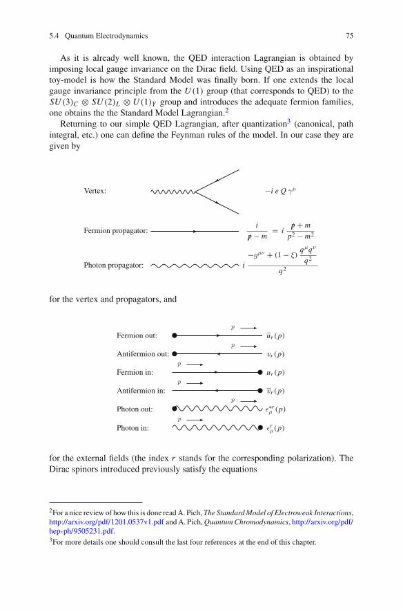
5.4 Quantum Electrodynamics 75

As it is already well known, the QED interaction Lagrangian is obtained byimposing local gauge invariance on the Dirac field. Using QED as an inspirationaltoy-model is how the Standard Model was finally born. If one extends the localgauge invariance principle from the U (1) group (that corresponds to QED) to theSU (3)C ⊗ SU (2)L ⊗ U (1)Y group and introduces the adequate fermion families,one obtains the the Standard Model Lagrangian.2

Returning to our simple QED Lagrangian, after quantization3 (canonical, pathintegral, etc.) one can define the Feynman rules of the model. In our case they aregiven by

Vertex: −i e Q γμ

Fermion propagator:i

/p − m= i

/p + m

p2 − m2

Photon propagator: i−gμν + (1 − ξ)

qμqν

q2

q2

for the vertex and propagators, and

Fermion out:p

ur (p)

Antifermion out:p

vr (p)

Fermion in:p

ur (p)

Antifermion in:p

vr (p)

Photon out:p

ε∗rμ (p)

Photon in:p

εrμ(p)

for the external fields (the index r stands for the corresponding polarization). TheDirac spinors introduced previously satisfy the equations

2For a nice review of how this is done readA. Pich,The Standard Model of Electroweak Interactions,http://arxiv.org/pdf/1201.0537v1.pdf andA. Pich,Quantum Chromodynamics, http://arxiv.org/pdf/hep-ph/9505231.pdf.3For more details one should consult the last four references at the end of this chapter.

76 5 Dirac Algebra

(/p − m

)ur (p) = 0, ur (p)

(/p − m

) = 0, (5.51)(/p + m

)vr (p) = 0, vr (p)

(/p + m

) = 0. (5.52)

Summing over the polarization of the spinors one finds the following relations

2∑

r=1

ur (p) ur (p) = (/p + m

),

2∑

r=1

vr (p) vr (p) = (/p − m

). (5.53)

These two results will turn out to be useful for calculating squared matrix elementsfor unpolarized fermions, as we shall shortly see with an example.

5.4.1 Unpolarized Transition Matrices

In this subsection we will use the previously Feynman rules to present the basicsof the scattering matrix calculations involving spinors and photons. Consider thefollowing process

e+(p1) e−(p2) → γ(k1) γ(k2). (5.54)

The corresponding Feynman diagrams are shown in Fig 5.1. The total squared tran-sition matrix will be given by

∣∣M∣∣2 = ∣∣M1∣∣2 + ∣∣M2

∣∣2 + 2Re M†1M2. (5.55)

Fig. 5.1 Feynman diagramsfor electron-positronannihilation to a pair ofphotons −iM1 =

p2

p1 k1

k2

p2 − k2

−iM2 =

p2

p1 k1

k2

p2 − k1

5.4 Quantum Electrodynamics 77

Here we shall only focus our attention on diagram (1). The rest of the calculationis left for the reader as an exercise. The transition matrix for the first diagram isgiven by

M1 = e2 Q2 εr∗μ (k1) εs∗

ν (k2)1

(p2 − k2)2 − m2 vr1(p1)

× γμ (/p2 − /k2 + m) γν ur2(p2). (5.56)

In the following we will explicitly calculate the hermitian conjugate of the spinorpart of this transition matrix:

(vr1 γμ (/p2 − /k2 + m) γν ur2

)† =

=(

v†r1 γ0 γμ (/p2 − /k2 + m) γν ur2

)†

= u†r2 γν† (/p

†2 − /k†2 + m) γμ† γ0† vr1

= u†r2 γ0 γν γ0 (γ0

/p2 γ0 − γ0 /k2 γ0 + m) γ0 γμ γ0 γ0 vr1

= ur2 γν (/p2 − /k2 + m) γμ vr1 . (5.57)

Thus, the hermitian conjugate of M1 is simply given by

M†1 = e2 Q2 εr

μ′(k1) εsν ′(k2)

1

(p2 − k2)2 − m2 ur2(p2)

× γν ′(/p2 − /k2 + m) γμ′

vr1(p1). (5.58)

The squared transition matrix for the first diagram then reads

∣∣M1∣∣2 = e4 Q4 εr∗

μ (k1) εrμ′(k1) εs∗

ν (k2) εsν ′(k2)

1

[(p2 − k2)2 − m2]2

× ur2 γν ′(/p2 − /k2 + m) γμ′

vr1 vr1 γμ (/p2 − /k2 + m) γν ur2 .

(5.59)

Introducing explicitly the matrix indices (the upper index for the rows and the lowerfor the columns and again, with summation over repeated indices understood) forthe spinors and the dirac matrices we find

78 5 Dirac Algebra

(ur2

)i

(γν ′)i

j

(/p2 − /k2 + m

) jk

(γμ′)k

l

(vr1

)l (vr1

)m

× (γμ

)mn

(/p2 − /k2 + m

)no

(γν

)op

(ur2

)p =

= (γν ′)i

j

(/p2 − /k2 + m

) jk

(γμ′)k

l

(vr1

)l (vr1

)m

× (γμ

)mn

(/p2 − /k2 + m

)no

(γν

)op

(ur2

)p (ur2

)i =

= Tr{γν ′

(/p2 − /k2 + m) γμ′vr1 vr1 γμ (/p2 − /k2 + m) γν ur2 ur2

}. (5.60)

Summing over the polarizations of the fermions and of the photons we obtain

∑

r,s,r1,r2

∣∣M1∣∣2 = e4 Q4 (−gμμ′) (−gνν ′)

1

[(p2 − k2)2 − m2]2

× Tr{γν ′

(/p2 − /k2 + m) γμ′(/p1 − m)

× γμ (/p2 − /k2 + m) γν (/p2 + m)}

(5.61)

The corresponding formulae needed for calculating cross sections and decay ratesare given in Chap.3.

Note that, when summing over the polarizations of the photon we have made theusual substitution

∑

r

εr∗μ (p) εr

ν(p) → −gμν . (5.62)

This can safely be done in QED due to the fact that it is an abelian gauge theory.The photon always couples to a conserved current and the non-physical polariza-tions do not contribute to the physical observables. For QCD, which is non-abelian,the previous substitution must be done with care. We shall discuss this in the nextsubsection.

5.4.2 Non Abelian Gauge Theories

Consider the following QCD process

q(p1) q(p2) → g(p3) g(p4). (5.63)

where qq stands for a quark-antiquark pair and g stands for gluon. For this processone has the same two diagrams from the previous section (with gluons substitutingthe photons and quarks substituting the electrons) plus a third one, that involves atriple gluon vertex (which is absent in QED). The complete set is shown in Fig. 5.2,

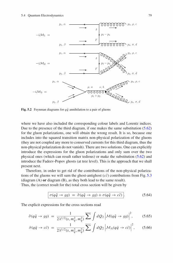
5.4 Quantum Electrodynamics 79

−iM1 =

p2, β

p1, α p3, ρ, c

p4, σ, d

p2 − p4

δ

δ′

−iM2 =

p2, β

p1, α p3, ρ, c

p4, σ, d

p2 − p3

δ

δ′

−iM3 =

p2, β

p1, α p3, ρ, c

p4, σ, d

p1 + p2

μ, a ν, b

Fig. 5.2 Feynman diagrams for qq annihilation to a pair of gluons

where we have also included the corresponding colour labels and Lorentz indices.Due to the presence of the third diagram, if one makes the same substitution (5.62)for the gluon polarizations, one will obtain the wrong result. It is so, because oneincludes into the squared transition matrix non-physical polarization of the gluons(they are not coupled any more to conserved currents for this third diagram, thus thenon-physical polarization do not vanish). There are two solutions. One can explicitlyintroduce the expressions for the gluon polarizations and only sum over the twophysical ones (which can result rather tedious) or make the substitution (5.62) andintroduce the Fadeev-Popov ghosts (at tree level). This is the approach that we shallpresent next.

Therefore, in order to get rid of the contributions of the non-physical polariza-tions of the gluons we will sum the ghost-antighost (cc) contributions from Fig. 5.3(diagram (A) or diagram (B), as they both lead to the same result).Thus, the (correct result for the) total cross section will be given by

σ(qq → gg) = σ(qq → gg) + σ(qq → cc) . (5.64)

The explicit expressions for the cross sections read

σ(qq → gg) = 1

2λ1/2(s, m2q , m2

q)

∑ ∫d Q2

∣∣∣M(qq → gg)

∣∣∣2, (5.65)

σ(qq → cc) = 1

2λ1/2(s, m2q , m2

q)

∑ ∫d Q2

∣∣∣MA(qq → cc)∣∣∣2, (5.66)

80 5 Dirac Algebra

−iMA =

p2, β

p1, α p3, c

p4, d

p1 + p2

μ, a ν, b

−iMB =

p2, β

p1, α p3, c

p4, d

p1 + p2

μ, a ν, b

Fig. 5.3 Feynman diagrams for qq annihilation to ghost-antighost

where we have introduced the spin and colour (Nc = 3) averaged sum

∑≡ 1

N 2c

1

(2 jq + 1)2∑

pol.

∑

col.

, (5.67)

and where

∣∣M(qq → gg)∣∣2 = ∣∣M1

∣∣2 + ∣∣M2∣∣2 + ∣∣M3

∣∣2 + 2ReM†1M2

+ 2ReM†2M3 + 2ReM†

1M3. (5.68)

When calculating these cross sections one must remember that d Q2 includes anidentical particles 1/2 symmetry factor for the cross section with gluons in the finalstate, whereas this factor does not exist for the cross section with ghosts in the finalstate (a ghost and an anti-ghost are not identical particles).

It is left as an exercise for the reader to explicitly check the following results(the needed Feynman rules in the Feynman gauge ξ = 1 are given in Fig. 5.4; thefermion-fermion-gluon vertex is proportional to the matrix elements (λa)αβ , whereλa are the Gell-Mann matrices, thus for the external fields the same Feynman rulesfrom QED are valid except, fermions must also have a colour label α, β, etc. andgluon polarization vectors must have a, b, etc. labels).4 For initial state masslessquarks we have (summation over repeated colour indices must not be understoodexcept if the symbol

∑is explicitly introduced)

4For a complete set of Feynman rules for QCD (and the SM in general) see J. C. Romao andJ. P. Silva, A resource for signs and Feynman diagrams of the Standard Model, Int. J. Mod. Phys.A 27 (2012) 1230025, http://arxiv.org/pdf/1209.6213.pdf

5.4 Quantum Electrodynamics 81

c

b

k

μ, a

− gs fabc kμ ,

α

β

μ, a

−i gs

(λa

2

)αβ

γμ ,

p, μ, a

q, ν, b

k, ρ, c

− gs fabc(gμν(p − q)ρ + gνρ(q − k)μ + gμρ(k − p)ν

),

μ, a ν, b

i−gμν

k2δab ,

α βi

/k + m

k2 − m2δαβ .

Fig. 5.4 Feynman rules needed for the qq → gg process

−i M1(α,β, c, d) = −i ερ∗c,r3(p3) εσ∗

d,r4(p4) vαr1(p1)γρ

× /p2 − /p4(p2 − p4)2

γσ uβr2(p2) g2s

∑

δ,δ′τ cαδ τd

δ′β δδδ′ , (5.69)

−i M2(α,β, c, d) = −i ερ∗c,r3(p3) εσ∗

d,r4(p4) vαr1(p1)γρ

× /p2 − /p3(p2 − p3)2

γσ uβr2(p2) g2s

∑

δ,δ′τdαδ τ c

δ′β δδδ′, (5.70)

82 5 Dirac Algebra

−i M3(α,β, c, d) = ερ∗c,r3(p3) εσ∗

d,r4(p4) vαr1(p1)γμuβ

r2(p2)(−g2s )

×(gνρ(k + p3)σ + gρσ(−p3 + p4)ν + gσν(−p4 − k)ρ

)

× −gμν

(p1 + p2)2∑

a,b

τaαβ f bcd δab , (5.71)

−i MA(α,β, c, d) = vαr1(p1)γμ uβ

r2(p2) (−g2s )−gμν

(p1 + p2)2

× p3,ν∑

a,b

τaαβ f bcd δab , (5.72)

where we have introduced the short-hand notation τaαβ = (λa/2)αβ . For the squared

transition matrix, when summing over the colours i.e.,

∑

α,β,c,d

∣∣M(α,β, c, d)∣∣2 , (5.73)

the following properties for the Gell-Mannmatrices λa and the totally antisymmetricstructure functions f abc (given by the commutation relation [τa, τb] = i f abcτ c) willturn out to be very useful

∑

α,β,c,d

∑

δ,δ′τ cαδ τd

δβ τdβδ′ τ c

δ′α = 1

16

∑

c,d

Tr{λcλdλdλc} = 16

3, (5.74)

∑

α,β,c,d

∑

δ,δ′τdαδ τ c

δβ τdβδ′ τ c

δ′α = 1

16

∑

c,d

Tr{λdλcλdλc} = −2

3, (5.75)

∑

α,β,c,d

∑

a,b

τaβα τb

αβ f bcd f acd = 1

4

∑

c,d

∑

a,b

Tr{λaλb} f bcd f acd = 12 , (5.76)

∑

α,β,c,d

∑

δ,b

τdδα τb

αβ τ cβδ i f bcd = 1

8

∑

c,d

∑

b

i f bcd Tr{λbλdλc} = −6. (5.77)

We shall only perform the explicit calculation for the first squared amplitude:

−i M1(α,β, c, d) = −i ερ∗c,r3(p3) εσ∗

d,r4(p4) vαr1(p1)γρ

× /p2 − /p4(p2 − p4)2

γσ uβr2(p2) g2s

∑

δ

τ cαδ τd

δβ, (5.78)

i M†1(α,β, c, d) = i ερ′

c,r3(p3) εσ′d,r4(p4) uβ

r2(p2)γσ′

× /p2 − /p4(p2 − p4)2

γρ′ vαr1(p1) g2s

∑

δ′τ cδ′α τd

βδ′ . (5.79)

5.4 Quantum Electrodynamics 83

Summing over the gluon and fermion polarizations

∑

ri

∣∣M1(α,β, c, d)∣∣2 = (−gρρ′

)(−gσσ′)g4st2

∑

δ,δ′τ cαδ τd

δβ τdβδ′ τ c

δ′α

× Tr{γσ′( /p2 − /p4)γρ′ /p1γρ( /p2 − /p4)γσ /p2}. (5.80)

Finally, summing over the colours, using (5.74–5.77), introducing the spin and colouraverage factors from (5.67), one obtains the following results

∑∣∣M1∣∣2 = g4s

32 u

27 t, (5.81)

∑∣∣M2∣∣2 = g4s

32 t

27 u, (5.82)

∑∣∣M3∣∣2 = −4 g4s

4 t2 + 3 u t + 4 u2

3 s2, (5.83)

∑∣∣MA∣∣2 = −g4s

2 t u

3 s2, (5.84)

and for the crossed terms

∑2ReM†

1M2 = g4s

(8 s

27

)s + t + u

t u= 0 , (5.85)

∑2ReM†

2M3 = g4s4 (s + t − u)

3 s, (5.86)

∑2ReM†

1M3 = g4s4 (s − t + u)

3 s. (5.87)

The final result for the total differential cross section is given by5

dσ(qq → gg)

dt= α2

s π

2 s2

[32

27

(t2 + u2

t u

)− 8

3

(t2 + u2

s2

) ], (5.88)

where we have introduced αs = g2s /4π, the strong coupling constant.

Further Reading

A. Pich, Quantum Chromodynamics, http://arxiv.org/pdf/hep-ph/9505231.pdfG. Dissertori, I.G. Knowles, M. Schmelling, Quantum ChromodynamicsA. Pich, The Standard Model of Electroweak Interactions, http://arxiv.org/pdf/1201.0537v1.pdf

5The result from Peskin and Schroeder for this cross section seems not to be correct, however ourresult agrees (except a 1/2 factor which they did not include) with R.K. Ellis, W.J. Stirling, B.R.Webber, QCD and Collider Physics.

84 5 Dirac Algebra

T. Muta, Foundations of Quantum ChromodynamicsJ.C. Romao, J.P. Silva, A resource for signs and Feynman diagrams of the standard model, Int. J.

Mod. Phys. A 27 (2012) 1230025, http://arxiv.org/pdf/1209.6213.pdfR.K. Ellis, W.J. Stirling, B.R. Webber, QCD and Collider PhysicsT.P. Cheng, L.F. Li, Gauge Theory of Elementary Particle Physics, (Oxford, 1984)L.H. Ryder, Quantum Field Theory, (Cambridge University Press, 1985)F. Mandl, G.P. Shaw, Quantum Field TheoryM. Kaku, Quantum Field Theory: A Modern Introduction.M.E. Peskin, D.V. Schroeder, An Introduction To Quantum Field Theory (Addison-Wesley Publish-

ing Company, San Francisco, 1995)

Chapter 6Dimensional Regularization. Ultravioletand Infrared Divergences

Abstract The cornerstone of Quantum Field Theory is renormalization. We shallspeak more about in the next chapters. Before, it is necessary to discuss the method.The best and most simple is, of course, dimensional regularization (doesn’t break thesymmetries, doesn’t violate the Ward Identities, preserves Lorentz invariance, etc.).When explained consistently, it becomes very simple and clear. Here, we shortlydiscuss ultraviolet (UV) and infrared (IR) divergenceswith a few examples.However,in Chap.8, we shall extensively treat one-loop two and three-point functions andanalyse many more examples of IR and UV divergences.

6.1 Master Integral

When calculating higher order quantum corrections (loop diagrams) one will findthat, normally, the loop integrals are divergent. In order to make sense out of thisdivergent integrals and be able to properly define finite observables one has to reg-ularize the divergent integrals (make them finite) and renormalize. In this chapterwe shall treat the regularization procedure. In the next chapter we shall talk aboutrenormalization.

In order to regularize the loop integrals, one can use different approaches i.e.,cut-off, Wilson regularization, dimensional regularization, etc. This last approach isthe one we shall treat in this chapter. It is the most adequate due to the fact that itpreserves all the symmetries of the theory. It consists in considering that the space-time dimension is not 4 but D = 4 + 2ε and work in the limit ε → 0. With thisconsideration all loop-integrals are finite. The general D-dimensional integral thatwe will always relate to (as we shall shortly see in the next sections) is

J (D,α,β, a2) ≡∫

d Dk

(2π)D

(k2)α

(k2 − a2)β, (6.1)

where D is the number of space-time dimensions, as we already mentioned. We caneasily demonstrate (see Appendix A) that it can be written in terms of the EulerGamma function as

© Springer International Publishing Switzerland 2016V. Ilisie, Concepts in Quantum Field Theory,UNITEXT for Physics, DOI 10.1007/978-3-319-22966-9_6

85

86 6 Dimensional Regularization. Ultraviolet and Infrared Divergences

J (D,α,β, a2) = i

(4π)D/2 (a2)D/2(−a2)α−β Γ (β − α − D/2)Γ (α + D/2)

Γ (β)Γ (D/2).

(6.2)

For z a complex number with Re(z) > 0 we have the following property of Γ (z)

Γ (z + 1) = zΓ (z). (6.3)

For n = 0, 1, 2, 3, . . . , it takes the form of the usual factorial function

Γ (n + 1) = n!. (6.4)

The function Γ (z) has simple poles at z = 0,−1,−2, . . . In the region −1 < ε < 0with ε ∈ R and |ε| � 1, we have the following Laurent expansion up to O(ε)

Γ (−ε) = −1

ε− γE + O(ε), (6.5)

where γE = 0.57721 . . . is the Euler-Mascheroni constant. Taking D = 4+ 2ε with−1 < ε < 0, |ε| � 1 (UV-divergent integrals in D = 4 dimensions are convergentin D < 4 dimensions) and power-expanding in ε, it is straightforward to find theexpression for the UV divergent function J (D, 0, 2, a2):

J (D, 0, 2, a2) = −i

(4π)2

(1

ε+ γE − ln(4π) + ln(a2) + O(ε)

). (6.6)

It will be useful to define the following quantity:

1

ε≡ 1

ε+ γE − ln(4π) . (6.7)

Because a in (6.6) has energy dimensions within the logarithm, we multiply anddivide the RHS of (6.6) by μ2ε, with μ a parameter with energy dimensions (calledthe renormalization scale), and use the expansion

μ−2ε = 1 − 2 ε ln(μ) + O(ε2), (6.8)

to finally obtain the following simple expression for J (D, 0, 2, a2)

J (D, 0, 2, a2) = −i

(4π)2μ2ε

[1

ε+ ln

( a2

μ2

)]+ O(ε) . (6.9)

6.1 Master Integral 87

We can easily relate all the UV divergent integrals to this one by using the recursionproperties of the Gamma function so practically one does not have to integrateever again over the four-momentum (except for some special cases where IRdivergences are also present). Some useful results are presented next.

6.2 Useful Results

Using theGamma function recursion properties we can find very useful the followingrelations

J(D, 0, 1, a2) =a2

D/2− 1J(D, 0, 2, a2)

J(D, 1, 1, a2) =a4

D/2− 1J(D, 0, 2, a2)

J(D, 1, 2, a2) =a2 D

D − 2J(D, 0, 2, a2)

J(D, 2, 2, a2) =a4(D + 2)

D − 2J(D, 0, 2, a2)

J(D, 1, 3, a2) =D

4J(D, 0, 2, a2)

(6.10)

As we shall see, all these results will be very useful in Chap.8. One can constructsimilar recursion relations for any values of α and β of our function J (D,α,β, a2)

with no additional complications.It is worth mentioning that the previous relations are general, meaning that they

are valid for any dimension D (D < 4 or D > 4). This can turn out to be usefulalso when treating IR divergences (IR divergent integrals in D = 4 dimensions areconvergent in D > 4 dimensions).

An example of integral that is finite in D = 4 dimensions is the following:

J (4, 0, 3, a2) = −i

32π2

1

a2 . (6.11)

When IR divergences are present we have to be a little bit more careful (with thisintegral) as we shall shortly see with an explicit example. Some other useful genericresults in D dimensions for the Dirac gamma matrices are the following:

gμνgμν = DID,

γμγνγμ = (2 − D)γν,

γμγνγσγμ = 4gνσ ID + (D − 4)γνγσ,

γμγνγσγργμ = −2γργσγν − (D − 4)γνγσγρ, (6.12)

88 6 Dimensional Regularization. Ultraviolet and Infrared Divergences

where ID is the identity matrix in D dimensions. The standard convention is to takeits trace equal to four:

T r{ID} = 4. (6.13)

Many more relations of this type involving gamma matrices are present all over theliterature. Some other interesting results that involve the function J (D,α,β, a2) arethe following:

∫d Dk

(2π)D

(k2)αkμ

(k2 − a2)β= 0,

∫d Dk

(2π)D

(k2)αkμkν

(k2 − a2)β= gμν

DJ (D,α + 1,β, a2)

(6.14)

(6.15)

Using the last result we can straightforwardly deduce another relation:

∫d Dk

(2π)D

(k · p)2

(k2 − a2)β=

∫d Dk

(2π)D

kμkν pμ pν

(k2 − a2)β

=∫

d Dk

(2π)D

pμ pν

(k2 − a2)β

gμνk2

D

= 1

D

∫d Dk

(2π)D

k2 p2

(k2 − a2)β

= p2

DJ (D, 1,β, a2). (6.16)

Thus, we have found the following equality in D dimensions

∫d Dk

(2π)D

(k · p)2

(k2 − a2)β=

∫d Dk

(2π)D

(p2/D)k2

(k2 − a2)β. (6.17)

The reader is highly encouraged to find the generalization of this result for (k · p)α

with α an arbitrary positive integer.

6.3 Example: Cancellation of UV Divergences

The following is a simple but very useful example of how the divergent parts of anintegral cancel and lead to a finite final result. Consider

Gμν =∫

d Dk

(2π)D

4kμkν − gμνk2

[k2 − a2]3 . (6.18)

6.3 Example: Cancellation of UV Divergences 89

The calculation is straightforward. Using (6.10) we obtain

Gμν = gμν( 4

D− 1

)J (D, 1, 3, a2)

= gμν( 4

D− 1

) D

4J (D, 0, 2, a2)

= gμν(

− ε

2

)J (D, 0, 2, a2) + O(ε2)

= gμν i

32π2 + O(ε). (6.19)

Taking D → 4 we obtain:

Gμν ≡∫

d Dk

(2π)D

4kμkν − gμνk2

[k2 − a2]3 = gμν i

32π2 . (6.20)

It is a common mistake to think that because the final result is finite in 4 dimensionswe could have made directly the substitution kμkν → gμνk2/4 instead of kμkν →gμνk2/D. Wrong! This integral consists in the sum of two parts that diverge in 4dimensions. Only after these two parts are summed, the final result turns out to befinite. Thus, the substitution kμkν → gμνk2/D is only valid if it gives rise to a finiteresult. In our case both parts are finite for D < 4 (and not D = 4) dimensions andtherefore, we must maintain D = 4 + 2ε until the sum of both parts is performed.

6.4 Feynman Parametrization

Usually we don’t find simple propagators as in (6.1), therefore we have to performsome manipulations over the denominators. The standard procedure is using theFeynman parametrization:

1

Aα Bβ= Γ (α + β)

Γ (α)Γ (β)

∫ 1

0dx

xα−1(1 − x)β−1

[Ax + B(1 − x)]α+β, (6.21)

1

Aα BβCγ= Γ (α + β + γ)

Γ (α)Γ (β)Γ (γ)

∫ 1

0dx

∫ 1

0dy x

× (xy)α−1[x(1 − y)]β−1(1 − x)γ−1

[Axy + Bx(1 − y) + C(1 − x)]α+β+γ. (6.22)

90 6 Dimensional Regularization. Ultraviolet and Infrared Divergences

For α = β = γ = 1 we simply get:

1

AB=

∫ 1

0dx

1

[Ax + B(1 − x)]2 , (6.23)

1

ABC=

∫ 1

0dx

∫ 1

0dy

2x

[Axy + Bx(1 − y) + C(1 − x)]3 . (6.24)

An useful alternative for (6.24) is the following:

1

ABC= 2

∫ 1

0dx

∫ 1

0dy

∫ 1

0dz

δ(1 − x − y − z)

[Ax + By + Cz]3

=∫ 1

0dy

∫ 1−y

0dz

2

[A(1 − y − z) + By + Cz]3 . (6.25)

For a generic n-point function one can use the generalized Feynman parametrizationgiven by:

1

Aα11 Aα2

2 . . . Aαnn

= Γ (α)

Γ (α1)Γ (α2) . . . Γ (αn)

∫ 1

0dx1

∫ 1

0dx2 . . .

∫ 1

0dxn

× xα1−11 xα2−1

2 . . . xαn−1n(

x1A1 + x2A2 + · · · + xn An

)α

× δ(1 − x1 − x2 − · · · − xn), (6.26)

where we have defined α ≡ α1 +α2 + · · ·+αn . Integrating over the δ-function, wefind

1Aα1

1 Aα22 .... Aαn

n=

Γ (α)Γ (α1)Γ (α2) ... Γ (αn)

×∫ 1

0dx1

∫ 1−x1

0dx2 ...

∫ 1−x1−x2−...−xn−2

0dxn−1

× xα1−11 xα2−1

2 ... xαn−1−1n−1 (1− x1 − ... − xn−1)αn−1

(x1A1 + x2A2 + ... + xn−1An−1 + (1− x1 − ... − xn−1)An

)α

(6.27)

Next we shall see a few rather simple examples of how these parametrizations canbe used. However in Chap.8, we shall use these parametrizations to calculate morecomplicated UV and IR divergent integrals.

It is worth mentioning that one can consider the analytical prolongation to thecomplex plane and use this last parametrization (6.27) for non-integer powers

6.4 Feynman Parametrization 91

of propagators. They appear when one wants integrate over the four-momentum,logarithmic functions that depend on the four-momentum. At the end of Chap. 8 weshall also take a simple two-loop example to see how this can be done.

6.5 Example: UV Pole

Let’s consider the following integral:

I μ ≡∫

d Dk

(2π)D

kμ

((p + k)2 − m2)k2. (6.28)

Using the parametrization in (6.23) with A = (p + k)2 − m2 and B = k2 we obtain

1

((p + k)2 − m2)k2=

∫ 1

0dx

1

[((p + k)2 − m2)x + k2(1 − x)]2

=∫ 1

0dx

1

[(k + px)2 − a2]2 , (6.29)

where we have defined a2 ≡ −p2x(1 − x) + m2x . Therefore I μ takes the form

I μ =∫ 1

0dx

∫d Dk

(2π)D

kμ

[(k + px)2 − a2]2

=∫ 1

0dx

∫d Dk

(2π)D

kμ − xpμ

[k2 − a2]2

= −pμ∫ 1

0xdx J (D, 0, 2, a2)

= pμ i

(4π)2μ2ε

∫ 1

0xdx

[1ε

+ ln( a2

μ2

)]

= pμ i

(4π)2μ2ε

[ 1

2ε+

∫ 1

0xdx ln

(−p2x(1 − x) + m2x

μ2

)](6.30)

(to get to the second line we shifted the integration variable k → k − x p).

6.6 Example: IR Poles

Consider the following integral

I =∫

d Dk

(2π)D

1

k2(k + p2)2(k − p3)2, (6.31)

92 6 Dimensional Regularization. Ultraviolet and Infrared Divergences

with p22 = p23 = 0. Thus our denominator in the limit of small k behaves like

1

k2(k2 + 2p2 · k)(k2 − 2p3 · k)

k2�−−→ 1

k2(2p2 · k)(2p3 · k). (6.32)

We can observe two types of infrared divergences present in the denominator of(6.32):

1. k → 0, which is called soft divergence,

2. p3 · k or p2 · k → 0, which is called collinear divergence. (6.33)

The integral that we are treating here will turn out to be only IR divergent, withoutUV divergences (a case where we find both types of divergences will be treated inChap.8). In order to treat these IR divergences, we shall consider the space-timedimensions to be D = 4 + 2ε′ with ε′ ∈ R, ε′ > 0 and ε′ � 1 (the IR divergentintegrals in 4 dimensions are convergent in D > 4 dimensions, as we have alreadymentioned). Using the Feynman parametrization (6.24) with A = k2 + 2p2 · k,B = k2 − 2p3 · k and C = k2, we find

I =∫ 1

0dx

∫ 1

0dy

∫d Dk

(2π)D

2x

[(k + p2xy − p3x(1 − y))2 − a2]3

=∫ 1

0dx

∫ 1

0dy

∫d Dk

(2π)D

2x

[k2 − a2]3

= 2∫ 1

0dx

∫ 1

0dyx J (D, 0, 3, a2), (6.34)

where a2 = −2(p2 · p3)x2y(1− y). Taking D → 4 as in (6.11) would give rise to aninfinity when integrating over the Feynman parameters, as we will see in a moment.Let’s write J (D, 0, 3, a2) in the form of (6.2):

I = −i

(4π)D/2Γ (3 − D/2)∫ 1

0dx

∫ 1

0dyx(a2)D/2−3

= −i

(4π)D/2Γ (3 − D/2)(−2p2 · p3)D/2−3

∫ 1

0dxx D−5

×∫ 1

0dy yD/2−3(1 − y)D/2−3. (6.35)

Using the Euler Beta function (A.17) we obtain the following result for our integral:

6.6 Example: IR Poles 93

I = −i

(4π)D/2Γ (3 − D/2)(−2p2 · p3)D/2−3Γ (D − 4)

Γ (D − 3)

Γ (D/2 − 2)Γ (D/2 − 2)

Γ (D − 4)

= −i

(4π)D/2

Γ (3 − D/2)

Γ (D − 3)(−2p2 · p3)

D/2−3Γ (D/2 − 2)Γ (D/2 − 2)

= −i

(4π)2(−2p2 · p3)

−1(4π)−ε′(−2p2 · p3)ε′ Γ (1 − ε′)

Γ (1 + 2ε′)Γ (ε′)Γ (ε′)

= i

(4π)2

1

2p2 · p3

(−2p2 · p34π

)ε′ Γ (1 − ε′)Γ (1 + 2ε′)

Γ 2(ε′). (6.36)

Of course, one could further expand using:

Γ (ε′) = 1

ε′ − γE + 1

12(π2 + 6γ2

E )ε′ + O(ε′2), (6.37)

Γ (1 ∓ ε′) = 1 ± γEε′ + 1

12(π2 + 6γ2

E )ε′2 + O(ε′3), (6.38)

(−1)ε′ = e±iπε′ = 1 ± iπε′ − π2ε′2

2. (6.39)

Thus, we observe that our result (6.36) is proportional to IR poles of the form 1/ε′and 1/ε′2. This is why taking the limit D → 4 as in (6.11), in (6.34) would havebeen wrong.

One could argue that in the first example we also have a propagator of the type∼1/k2, which goes to infinity as k goes to zero. Therefore one should find IR diver-gences in this case also. It turns out, however, that it is not the case. It is clear thatwhen integrating over x , the expression (6.30) does not diverge. This expression isdivergent ifm2 = p2 = 0, however this specific case will be treated in Chap. 8. Thus,any potential IR divergence must be treated carefully. As we can see, after doing thecalculation, the IR divergence might actually not be there.

Further Reading

A. Pich, The Standard Model of Electroweak Interactions. http://arxiv.org/pdf/1201.0537v1.pdfA. Pich, Class Notes on Quantum Field Theory. http://eeemaster.uv.es/course/view.php?id=6M. Kaku, Quantum Field Theory: A Modern IntroductionM. Srednicki, Quantum Field TheoryM.E. Peskin, D.V. Schroeder, An Introduction to Quantum Field Theory (Addison-Wesley Publish-ing Company, San Francisco, 1995)

K. Kannike, Notes on Feynman Parametrisation and the Dirac Delta Function. http://www.physic.ut.ee/~kkannike/english/science/physics/notes/feynman_param.pdf

S. Pokorsky, Gauge Field TheoriesL.H. Ryder, Quantum Field Theory (Cambridge University Press, Cambridge, 1985)T.P. Cheng, L.F. Li,Gauge Theory of Elementary Particle Physics (OxfordUniversity Press, Oxford,1984)

F. Mandl, G.P. Shaw, Quantum Field Theory

Chapter 7QED Renormalization

Abstract This chapter is intended to present the standard renormalization algorithmto all orders in perturbation theory in a simple transparent manner. The calculationsare made as explicit as possible, in order to clarify many of the confusions that mayarise when treating this topic. We will restrict our attention to the most academicexample,which is (inmy opinion) theQEDLagrangian.We shall use the dimensionalregularization approach in D = 4+ 2ε dimensions (ε < 0) in order to regularise theUV divergences (as it is nicely explained in the previous chapter). Afterwards weshall take an explicit one-loop example and introduce the two usual renormalizationschemes, the M S and the on-shell scheme. A few clarifying notions on tadpoles arealso given at the end of the chapter.

7.1 QED Lagrangian

The QED Lagrangian written in terms of the bare (non physical) fields, masses,coupling constant and gauge parameter reads

LQE D = −1

4F (0)

μν Fμν(0) − 1

2ξ(0)

(∂μ Aμ

(0)

)2 + iψ(0)

γμ∂μψ(0)

− m0ψ(0)

ψ(0) − e0Q A(0)μ ψ

(0)γμψ(0) (7.1)

When including loop corrections the bare parameters will be replaced systematicallyby physical parameters of the renormalized theory as we shall see in this section. Westart by analysing the perturbative corrections to all orders to propagators, vertex,and fields.

7.2 Fermionic Propagator, Mass and Field Renormalization

The relevant diagrams for renormalization are the one particle irreducible diagrams.A one particle irreducible diagram (1PI) is one that, by cutting an internal line is nolonger connected. The 1PI fermionic self-energy diagrams that are needed for the

© Springer International Publishing Switzerland 2016V. Ilisie, Concepts in Quantum Field Theory,UNITEXT for Physics, DOI 10.1007/978-3-319-22966-9_7

95

96 7 QED Renormalization

fermionic propagator correction are schematically shown below:

i Σ(/p, ζ0) =

Σ = +++ ...

p

where we have introduced the short-hand notation ζ0 ≡ (m0, α0, ξ0) for the bareparameters. For the renormalized physical parameters we shall use ζ ≡ (m, α, ξ).The fully dressed propagator is given by the Dyson summation:

i S(/p, ζ0) =

= + ...+ ΣS + Σ Σ

Explicitly the previous sum reads:

i S(/p, ζ0) = i S(0)(/p, ζ0) + i S(0)(/p, ζ0)(i Σ(/p, ζ0)

)i S(0)(/p, ζ0) + · · · ,

(7.2)

where i S(0)(/p, ζ0) = i

/p − m0is the fermionic tree-level propagator. We obtain

S(/p, ζ0) = 1

/p − m0− Σ(/p, ζ0)

(/p − m0)2+ · · · = 1

/p − m0 + Σ(/p, ζ0). (7.3)

We will now define the Z2 renormalization constant that relates the bare (non-renormalized,UV-divergent) propagator S(/p, ζ0)with the renormalizedone SR(/p, ζ)

that contains only the regular (renormalized, UV finite) parts of the self-energy(denoted as Σ R) and that depends on the physical (renormalized) parameters m andα and ξ:

S(/p, ζ0) = 1

/p − m0 + Σ(/p, ζ0)≡ Z2 SR(/p, ζ) = Z2

/p − m + Σ R(/p, ζ). (7.4)

For the mass renormalization the standard procedure is to define the following renor-malization constants:

m ≡ m0 + δm ≡ Z2 Z−14 m0. (7.5)

Using (7.4) we are now able to relate the renormalized fermionic fields ψ(x) withthe bare ones ψ(0)(x) with the help of the time-ordered product:

T(ψ(0)(x),ψ (0)(y)

)∼ i

/p − m0 + · · · = i Z2

/p − m + · · · ∼ Z2 T(ψ(x),ψ(y)

).

(7.6)

7.2 Fermionic Propagator, Mass and Field Renormalization 97

We obtain thus, the following relations:

ψ(0)(x) = Z1/22 ψ(x), ψ (0)(x) = Z1/2

2 ψ(x). (7.7)

Next we move on to the analysis of the bosonic propagator and field renormal-ization.

7.3 Bosonic Propagator and Field Renormalization

The 1PI diagrams that contribute to the photon self energy are given by:

i Πμν(q2, ζ0) =

Πμν = + + ...+

q

Due to gauge invariance qμΠμν = qν Πμν = 0, therefore these 1PI diagrams mustnecessarily have the form

Πμν(q2) = (−gμνq2 + qμqν) Π(q2), (7.8)

with Π(q2) a Lorentz scalar. The Dyson summation for the photon propagator isthen given by:

i Dμν(q2, ζ0) =

= + + ...+Πμν Πμν ΠμνDμν

The explicit expression for the previous sum is:

i Dμν(q2, ζ0) = i Dμν(0)(q

2, ζ0) + i Dμλ(0)(q

2, ζ0)(

iΠλρ(q2, ζ0)

)i Dρν

(0)(q2, ζ0) + · · · ,

(7.9)

where i Dμν(0)(q

2, ζ0) = i−gμν + (1 − ξ0)qμqν/q2

q2 is the tree-level photon propaga-

tor. The second term of this sum gives:

Dμλ(0)(q

2, ζ0)Πλρ(q2, ζ0) Dρν

(0)(q2, ζ0) = 1

q2

(− gμν + qμqν

q2

)Π(q2, ζ0).

(7.10)

98 7 QED Renormalization

Therefore the complete Dyson summation is finally given by:

Dμν(q2, ζ0) = 1

q2

{(−gμν + qμqν

q2

) (1 − Π(q2, ζ0) + · · ·

)− ξ0

qμqν

q2

}

= 1

q2

{(−gμν + qμqν

q2

)1

1 + Π(q2, ζ0)− ξ0

qμqν

q2

}. (7.11)

Now, as we did before, we relate Dμν(q2, ζ0) with the renormalized propagatorDμν

R (q2, ζ) by defining another renormalization constant Z3 as

Dμν(q2, ζ0) ≡ Z3DμνR (q2, ζ) = Z3

q2

{(−gμν + qμqν

q2

)1

1 + ΠR(q2, ζ)− ξ

qμqν

q2

},

(7.12)

where ΠR is the regular part of the self-energy function from (7.8). Thus we get tothe following relations:

ξ0 = Z3 ξ,1

1 + Π(q2, ζ0)= Z3

1 + ΠR(q2, ζ). (7.13)

Again, using the time-ordered product we obtain the expression for the renormalizedphoton field

Aμ0 (x) = Z1/2

3 Aμ(x). (7.14)

The only thing we have left to complete the renormalization procedure is to analysethe vertex correction and the coupling constant renormalization.

7.4 Vertex Correction

The vertex correction to all orders in perturbation theory is schematically given by:

−i e0 Q Λμ(pi, ζ0) =

= +Λμp1

p2

p3

+ + ...

The complete vertex comes from summing the tree level one and the previous cor-rections:

7.4 Vertex Correction 99

−i e0 Q Γ μ(pi, ζ0) =

= + ΛμΓμ

Simplifying the −i e0 Q common factor, this sum simply reads:

Γ μ(pi , ζ0) = γμ + Λμ(pi , ζ0). (7.15)

The Z1 constant that renormalizes the vertex is defined as follows:

Γ μ(pi , ζ0) = 1

Z1Γ

μR (pi , ζ) = 1

Z1

(γμ + Λ

μR(pi , ζ)

). (7.16)

where ΓR and ΛR are (using the same notation as previously) regular (UV-finite)quantities. With the previous definition we can relate the bare coupling e0 with therenormalized one:

e0 Γ μ(pi , ζ0) = e0Z1

ΓμR (pi , ζ) ≡ e′ Γ μ

R (pi , ζ). (7.17)

We could be tempted to think that e′ is the renormalized coupling constant but that’snot really true. We must carefully look at the vertex diagram and realize that wehave three external fields that also need renormalization. We have a bosonic field,therefore we must multiply e′ by Z1/2

3 and we have two fermion fields, therefore weneed to also multiply by a Z2 term. The renormalized coupling is then given by:

e ≡ e0Z1

Z2 Z1/23 = e′ Z2 Z1/2

3 . (7.18)

We can demonstrate that the gauge invariance of the Lagrangian implies Z1 = Z2.Thus, we finally obtain the simple relations between e and α (where α = e2/4π)and the correspondent bare quantities

e = e0 Z1/23 ⇒ α = Z3α0. (7.19)

7.5 Renormalization to All Orders

To sum up, we have found the following relations between the bare and renormalizedquantities

ψ(0) = Z1/22 ψ, Aμ

0 = Z1/23 Aμ, e0 = Z−1/2

3 e,

ξ0 = Z3ξ, m0 = m − δm = Z4Z−12 m. (7.20)

100 7 QED Renormalization

Now we can re-write the original Lagrangian in terms of the renormalized physicalquantities using the Zi renormalization constants that we have defined in the previoussections:

LQE D = −1

4F (0)

μν Fμν(0) − 1

2ξ(0)

(∂μ Aμ

(0)

)2 + iψ(0)

γμ∂μψ(0)

− m0ψ(0)

ψ(0) − e0Q A(0)μ ψ

(0)γμψ(0)

= −Z31

4Fμν Fμν − 1

2ξ(∂μ Aμ)2 + Z2 iψγμ∂μψ

− Z4mψψ − Z1eQ Aμψγμψ

= −1

4Fμν Fμν − 1

2ξ(∂μ Aμ)2 + iψγμ∂μψ

− mψψ − eQ Aμψγμψ

− δ31

4Fμν Fμν + ψ(iδ2 /∂ − δ4m)ψ − δ1 eQ Aμψγμψ (7.21)

To get to the last equality we separated the Zi terms into their tree-level value 1, andthe loop contributions δi :

Zi = 1 + δi . (7.22)

The terms of the Lagrangian that are proportional to δi are called counterterms andthey guarantee that our theory has no more ultraviolet divergences at any order inperturbation theory. One should note that the renormalization process doesn’t consistin just adding counterterms to the Lagrangian in order to subtract infinities but in asystematic order by order process which is permitted by our reinterpretation of thebare and physical quantities of the Lagrangian. After including the quantum correc-tions and renormalizing something else happened. The renormalized quantities arenow renormalization scale (μ) dependent. Thus, one needs to solve the renormaliza-tion group equations (see Appendix B) in order to obtain their evolution (running)with the scale.

Our Feynman rules of the theory can now be written in terms of the renormalizedquantities both in the multiplicative or the counterterm approach. For the multiplica-tive approach, taking a quick look at the Lagrangian one finds the following Feynmanrules

7.5 Renormalization to All Orders 101

−Z1 i e Q γμ

i

Z2 /p − Z4 m

i

Z3

−gμν + (1 − Z3 ξ)qμqν

q2

q2

Therefore, when summing the higher order vertex corrections or performing theDyson resummation for the propagators (in terms of the previously introduced Feyn-man rules) one will directly obtain the renormalized quantities.

If one chooses the counterterm approach, the complete set of Feynman rules aregiven by the old ones (this time in terms of renormalized quantities)

−i e Q γμ

i

/p − m

i−gμν + (1 − ξ)

qμqν

q2

q2

plus three extra ones that account for the counterterms ∼ δi :

−i e Q γμ δ1

i(δ2 /p − δ4m)

i δ3 (−gμνq2 + qμqν)

Thus, when calculating higher order quantum corrections, the inclusion of the coun-terterms will guarantee the finiteness of our result. Considering for simplicity justone-loop graphs, diagrammatically this translates into:

102 7 QED Renormalization

+ = i ΠR(q2, ζ)

+ = i ΣR(/p, ζ)

+ = −i e Q ΛμR(pi , ζ)

In the following, we shall study the divergent parts of the one-loop diagramsand explicitly introduce the counterterms of the theory using the two most commonrenormalization schemes, the M S and the on-shell (OS) scheme.

7.6 One-Loop Renormalization Example

At one-loop level the fermion self-energy is given by:

i Σ(/p, ζ0) =

At this order we keep corrections of O(α) and drop all the higher order terms,therefore we can introduce the simplified notation:

Σ(/p, ζ0) ≈ Σ(/p, ζ) ≡ Σ(/p). (7.23)

Same consideration is valid for the bosonic self-energy and the vertex correction,therefore we shall drop the ζ0, ζ notation in this section. Returning to the fermionicself-energy, it is useful to make the following split

Σ(/p) = Σ1(p2) + (/p − m0)Σ2(p2) ≈ Σ1(p2) + (/p − m)Σ2(p2), (7.24)

where the last approximation is valid only at the one-loop level. The functionsΣ1(p2)and Σ2(p2) are two Lorentz scalars given by

Σ1(p2) = m αμ2ε

4π

(3

ε+ · · ·

)≡ Σε

1 + Σ R1 (p2), (7.25)

Σ2(p2) = ξ αμ2ε

4π

(−1

ε+ · · ·

)≡ Σε

2 + Σ R2 (p2), (7.26)

7.6 One-Loop Renormalization Example 103

where 1/ε ≡ 1/ε + γE − ln(4π) as defined in the previous chapter. The functionsΣε

i (i = 1, 2) are the parts of the self energy that contain the UV-divergent term1/ε and a constant that is determined by the renormalization scheme; Σ R

i are theregular parts of the self-energies as usual. Performing the Dyson summation for thefermionic propagator, this time including only one-loop 1PI diagrams

i S(/p) =

+= + + ...S

we obtain:

S(/p) = 1

/p − m0 + Σ(/p)≡ Z2 SR(/p) = Z2

/p − m + Σ R(/p). (7.27)

We can now in calculate Z2 up to order α in perturbation theory. Recalling thatm = m0 + δm, is the finite renormalized mass, then:

Z2 = /p − m + Σ R

/p − m0 + Σ= (/p − m)

(1 + Σ R

2

) + Σ R1

/p − m + δm + Σ

≈ (/p − m)(1 + Σ R

2

) + Σ R1

/p − m

(1 − δm + Σ

/p − m

)

=(1 + Σ R

2 + Σ R1

/p − m

) (1 − δm + Σ1

/p − m− Σ2

)

≈ 1 + Σ R2 + Σ R

1 − δm − Σ1

/p − m− Σ2

= 1 − Σε2 − Σε

1 + δm

/p − m. (7.28)

The renormalization constants are momentum independent, thus:

δm = −Σε1, Z2 = 1 − Σε

2. (7.29)

Previously we have introduced the Z4 constant as

m = m0 + δm = m0 − Σε1 ≡ Z2Z−1

4 m0, (7.30)

therefore

Z4 ≈ 1 − Σε2 + Σε

1

m0≈ 1 − Σε

2 + Σε1

m, (7.31)

104 7 QED Renormalization

where the last approximation is only valid at the one-loop order. We shall now moveon to the analysis of the one-loop photon self energy:

i Πμν(q2) =

As we have already mentioned, the expression of Πμν(q2) can be factorized in thegauge invariant form:

Πμν(q2) = (−gμνq2 + qμqν)Π(q2). (7.32)

The function Π(q2) is given by

Π(q2) = −α4

3

μ2ε

4π

[1ε

+ · · ·]

≡ Πε + ΠR(q2). (7.33)

We have decomposed as usual Π(q2) into an UV divergent (Πε) and a regular (ΠR)part. Performing the Dyson summation

i Dμν(q2) =

= + + ...Dμν +

we get:

ξ0 = Z3 ξ,1

1 + Π(q2)= Z3

1 + ΠR(q2). (7.34)

Up to order α, the Z3 renormalization constant is given by

Z3 = 1 + ΠR

1 + Π≈ (1 + ΠR)(1 − ΠR − Πε) ≈ 1 − Πε. (7.35)

Finally, the one-loop vertex correction is simply given by:

−i e0 Q Λμ(pi) =p1

p2

p3

The vertex function Λμ(pi ) explicitly reads

Λμ(pi ) = αμ2ε

4π

{γμ

[−ξ

1

ε+ · · ·

]+ · · ·

}. (7.36)

7.6 One-Loop Renormalization Example 105

We can decompose as usual Λμ into its finite (ΛR) and UV-divergent (Λε) parts:

Λμ(pi ) = Λμε + Λ

μR(pi ), with Λμ

ε = γμ Λε. (7.37)

Summing the one loop correction to the tree-level vertex one obtains

−i e0 Q Γ μ(pi) =

= +Γμ

Simplifying the −i e0 Q common factor we have

Γ μ(pi ) = γμ + Λμ(pi ). (7.38)

Introducing the Z1 renormalization constant

Γ μ = γμ(1 + Λε) + ΛμR = 1

Z1Γ

μR = 1

Z1(γμ + Λ

μR), (7.39)

up to order α we obtain

Z1

(γμ(1 + Λε) + Λ

μR

)≈ Z1γμ(1 + Λε) + Λ

μR = γμ + Λ

μR . (7.40)

Thus

Z1 = 1 − Λε. (7.41)

In conclusion, the one-loop level QED renormalization constants are given by:

Z1 = 1 − Λε ⇒ δ1 = −Λε

Z3 = 1 − Πε ⇒ δ3 = −Πε

Z2 = 1 − Σε2 ⇒ δ2 = −Σε

2

Z4 = 1 − Σε2 + Σε

1/m ⇒ δ4 = −Σε2 + Σε

1/m (7.42)

with Z1 = Z2 therefore, Σε2 = Λε, as it can be explicitly checked.

It is worth making the following comment. As the photon always couples toconserved currents, the qμqν part of the propagator will always vanish when calcu-lating physical observables. Thus, one can simplify the renormalization procedureby choosing for example the Feynman gauge (ξ = 1) for the tree-level photonpropagator and, when summing higher order corrections, simply ignore the qμqν

106 7 QED Renormalization

terms. However, in this chapter I preferred giving the full formal renormalizationprescription.

7.6.1 M S Renormalization Scheme

The split we have just made between the UV divergent and the regular parts of theprevious functions is somewhat ambiguous. A given choice of this separation definesa renormalization scheme. For the M S scheme, the Zi renormalization constants onlyabsorb the 1/ε terms (plus no other constant) thus, they are simply given by:

Z2 = Z1 = 1 + α

4πμ2ε ξ

1

ε, (7.43)

Z3 = 1 + α

3πμ2ε 1

ε, (7.44)

Z4 = 1 + α

4πμ2ε (3 + ξ)

1

ε. (7.45)

Next we present the on-shell (OS) renormalization scheme.

7.6.2 On-Shell Renormalization Scheme

For this renormalization scheme the expressions of the counterterms are not asstraightforward to obtain as previously. In the OS scheme the renormalization coun-terterms must guarantee that the the poles of the renormalized propagators coincidewith the physical masses (m for the fermion and 0 for the photon in our case). Thestandard procedure is shown next.

Let’s take a look at the fermionic propagator (7.27) and make a Taylor expansionaround the pole (/p = m)

1

/p − m0 + Σ(/p)≈ 1

/p − m0 + Σ(m) + (/p − m)Σ ′(m)

≈ Z2

/p − m + Σ R(m) + (/p − m)Σ ′ R(m), (7.46)

where Σ ′(m) is the short-hand notation for

Σ ′(m) = d

d /pΣ(/p)

∣∣∣∣/p=m

(7.47)

7.6 One-Loop Renormalization Example 107

(when differentiating with respect to /p one must take into account that p2 = /p2,thus dp2/d /p = 2/p). Imposing that Σ R(m) = 0 and Σ ′ R

(m) = 0 (the pole of therenormalized propagator is given by the physical mass with same residue 1 as thetree-level propagator) we have

1

/p − m + δm + Σ(m) + (/p − m)Σ ′(m)≈ Z2

/p − m. (7.48)

Choosing the mass counterterm to be

δm = −Σ(m), (7.49)

we obtain the Z2 renormalization constant at one-loop level

Z2 = 1 − Σ ′(m) = Z1. (7.50)

Thus, after having defined the previous renormalization constants, looking again at(7.27) we find that for the on-shell scheme, at the one-loop level, the regular part ofthe self-energy is given by

Σ R(/p) = Σ(/p) − Σ(m) − (/p − m) Σ ′(m). (7.51)

Looking at (7.34), for q2 = 0 we have the following relation

1

1 + Π(0)= Z3

1 + ΠR(0). (7.52)

Imposing the on-shell condition ΠR(0) = 0 we obtain the Z3 renormalization con-stant:

Z3 = 1 − Π(0). (7.53)

As in the previous case, looking again at (7.34), for arbitrary q2, the regular part ofthe bosonic self-energy reads:

ΠR(q2) = Π(q2) − Π(0). (7.54)

Any other condition imposed on the vertex would be redundant. As we have alreadymentioned many times, gauge invariance fixes Z1 = Z2, and therefore the value ofthe regular part of vertex function is also fixed by the previous on-shell conditions.

So farwehave supposed that the fermionof the theory is a stable particle i.e., it doesnot decay into lighter particles. If the fermion can however, decay (a muon for exam-ple), we must slightly modify the previous on-shell conditions for the fermion massand wave function renormalization (besides of course, including and renormalizing

108 7 QED Renormalization

the new terms of the Lagrangian). If p2 ≥ ( ∑i mi

)2, where mi are the masses ofthe particles in which the fermion can decay, then Σ(/p) develops an imaginary partthat is UV-finite (thus, it needs no renormalization). Separating the self energy intothe real and imaginary parts, (7.27) takes the form:

1

/p − m0 + ReΣ(/p) + i ImΣ(/p)= Z2

/p − m + ReΣ R(/p) + i ImΣ(/p). (7.55)

At one-loop order:

/p − m0 + ReΣ(/p) + i ImΣ(/p) = Z−12

(/p − m + ReΣ R(/p) + i ImΣ(/p)

)

≈ (1 − δ2)(/p − m) + ReΣ R(/p) + i ImΣ(/p).

(7.56)

Thus, at this order in perturbation theory

1

/p − m0 + ReΣ(/p)≈ Z2

/p − m + ReΣ R(/p). (7.57)

Using the same procedure as previously (making a Taylor expansion around the pole,this time only for the real part of the self-energy) we obtain

δm = −ReΣ(m), Z2 = 1 − ReΣ ′(m) = Z1. (7.58)

and

Σ R(/p) = ReΣ(/p) − ReΣ(m) − (/p − m) ReΣ ′(m) + i ImΣ(/p). (7.59)

The imaginary part of the self-energy shifts the pole of the propagator from the realto the imaginary axis. When reaching the on-shell region (p2 = m2), this imaginarypart takes the well known Breit-Wigner form

i ImΣ(m) = i m Γ, (7.60)

whereΓ is the total decay rate of the fermion (seeChap. 12 for details and demonstra-tion). This has a physical consequence. It is obviously the reasonwhy, experimentally,a resonance doesn’t peak as a delta function, but has a finite width.

As the Imaginary part of the self-energy does not affect the UV-divergent poles,the M S-scheme must not be modified for unstable particles.

7.7 Renormalization and Tadpoles 109

7.7 Renormalization and Tadpoles

Depending on the quantization procedure one might have to deal with tadpoles. Thistopology is shown in Fig.7.1. The contribution of this diagram modifies the vacuumexpectation value (vev) of the field as we shall see in a moment. If one uses thecanonical quantization procedure with normal ordered products of fields one willnever find this topology as it involves the contraction of two fields in the same space-time point. If one uses the path integral quantization, one finds the same topologiesfor the connected diagrams as in the previous case plus tadpoles. Thus, when dealingwith propagator corrections one will find topologies like

which are not proper 1PI diagrams. Do not confuse tadpole topologies with theseagull topologies that are shown below

The seagull topologies (which are oftenly also called tadpoles by many authors) areproper 1PI diagrams and must be included into the renormalization algorithm.

Returning to tadpoles, in order to get rid of these contributions one usually rede-fines the field’s vev and generates a counter-term in the Lagrangian that cancelsthe tadpoles to all orders in perturbation theory. We can explicitly see this with thefollowing example. Consider the φ3 Lagrangian

L(x) = 1

2∂μφ(x)∂μφ(x) − 1

2m2φ2(x) − λ

3!φ3(x). (7.61)

Including one-loop order corrections one finds that the vev of φ is given by

〈0|φ(x)|0〉 = t

m2 . (7.62)

Fig. 7.1 Tadpole topology

i t =

110 7 QED Renormalization

with t shown in Fig. 7.1. Defining a new field φ′(x) = φ(x)− t/m2, one immediatelyfinds

〈0|φ(x)′|0〉 = 〈0|φ(x)|0〉 − t

m2 〈0|0〉 = 0. (7.63)

Rewriting the Lagrangian (only the parts that correspond to the free field, obviouslythe interaction term must not be modified as it was already used to calculate t) interms of the field φ′(x) one generates a counterterm of the type Lct (x) = −φ′(x) twhich cancels the tadpole contributions.1 Diagrammatically

+ ct = 0

for the vev and

+

ct

= 0

for the propagator correction. So, in this simple φ3 model one does not even needto bother in calculating tadpoles. They simply cancel when the counterterms areadded. Thus, one can consider as usual, just 1PI diagrams when renormalizing theLagrangian. Defining the Zi renormalization constants as

m20 = Zm m2 φ0 = Z1/2

φ φ, λ0 = Zλ λ, (7.64)

and dropping the primed notation one finally finds the following Lagrangian in termsof the renormalized quantities

L = Zφ1

2∂μφ ∂μφ − Zm Zφ

1

2m2 φ2 − Zλ Z3/2

φ

λ

3! φ3 − t φ. (7.65)

This is however, a toy model. Things are not that simple in the electroweak sectorof the Standard Model. The Higgs field will generate tadpoles. After performing asimilar redefinition one will generate a similar counterterm. However, there will beterms in the Lagrangian that will generate diagrams of the type

cthh

tadpole

1One also generates a constant term −t2/2m2 that can be safely dropped as it will play no role inthe interactions.

7.7 Renormalization and Tadpoles 111

which must be included in the renormalization process (they also play an importantrole in the Ward identities). It is also worth mentioning that tadpoles also play animportant role is one wishes to define gauge independent mass counterterms,2 whichis not mandatory (mass counterterms are not observables) but it is a nice feature thatone can exploit. More on tadpoles and theWard identities in the StandardModel willbe treated in Chap.9.

Finally, tadpoles for vector fields (massive or massless) in the Standard Modelalways vanish, as they would simply break Lorentz invariance (which is one of thefundamental symmetries of the theory).

Further Reading

M. Kaku, Quantum Field Theory: A Modern Introduction (Oxford University Press, New York,1993)

A. Pich, Class Notes on Quantum Field Theory. http://eeemaster.uv.es/course/view.php?id=6M. Srednicki, Quantum Field Theory (Cambridge University Press, New York)L.H. Ryder, Quantum Field Theory (Cambridge University Press, New York, 1985)T.P. Cheng, L.F. Li, Gauge Theory of Elementary Particle Physics (Oxford University Press, NewYork, 1984)

F. Mandl, G.P. Shaw, Quantum Field Theory (Chichester, New York, 1984)

2The full details at one and two-loop level are very nicely given in S. Actis, A. Ferroglia, M. Passeraand G. Passarino, Two-Loop Renormalization in the Standard Model. Part I: Prolegomena, Nucl.Phys. B 777 (2007) 1, http://arxiv.org/pdf/hep-ph/0612122.pdf

Chapter 8One-Loop Two and Three-Point Functions

Abstract In this chapter we present a few relevant calculations of one-loop, oneand two-point (scalar, vector and tensor) functions. IR and UV divergences areextensively treated. One example of IR-pole cancellation is presented. The two andthree-body phase space integrals in D dimensions, needed for the calculation of IRdivergent cross sections are also given. Last, the usage of the generic parametriza-tion (6.27) for non-integer powers of propagators (which appear when one needs tointegrate over the four-momentum, logarithmic functions that depend on the four-momentum) is shown with a simple two-loop example. With the tools given here,the reader should find straightforward to construct any higher order scalar or tensorintegral for any N-point function at one-loop level.

8.1 Two-Point Function

We shall begin this chapter by studying the two-point function. The reader is highlyencouraged to perform all the calculations step-by-step and reproduce the resultsobtained here.

The distribution of momenta is shown in Fig. 8.1. The exterior legs are not neces-sarily on-shell (meaning that we shall not use the equality p2i = m2

i ). All the massesare considered to be different. The denominator of this two-point function is

1

[(k + p1)2 − m2](k2 − M2). (8.1)

The Feynman parametrization that we will use in this case is (6.23). Taking A =[(k + p1)2 − m2] and B = (k2 − M2) we obtain:

1

[(k + p1)2 − m2](k2 − M2)=

∫ 1

0dx

1

D2 . (8.2)

© Springer International Publishing Switzerland 2016V. Ilisie, Concepts in Quantum Field Theory,UNITEXT for Physics, DOI 10.1007/978-3-319-22966-9_8

113

114 8 One-Loop Two and Three-Point Functions

p1, m1

k + p1, m

k, M

p1, m1

Fig. 8.1 Distribution of masses and momenta for the two-point function

where D has the following expression:

D = (k + p1x)2 − a2, a2 ≡ p21x(x − 1) + m2x + M2(1 − x). (8.3)

The first integral that we shall deal with is the scalar integral:

I1 ≡∫

d Dk

(2π)D

1

[(k + p1)2 − m2](k2 − M2). (8.4)

Using the previous results for dimensional regularization from Chap.6 we find

I1 =∫ 1

0dx

∫d Dk

(2π)D

1

[(k + p1x)2 − a2]2

=∫ 1

0dx

∫d Dk

(2π)D

1

[k2 − a2]2

=∫ 1

0dx J (D, 0, 2, a2)

= −i

(4π)2μ2ε

[1

ε+

∫ 1

0dx ln

( a2

μ2

)], (8.5)

where, to get to the second line we shifted the integration variable k → k − x p1.The second integral that we shall calculate is the vector integral:

I μ2 ≡

∫d Dk

(2π)D

kμ

[(k + p1)2 − m2](k2 − M2). (8.6)

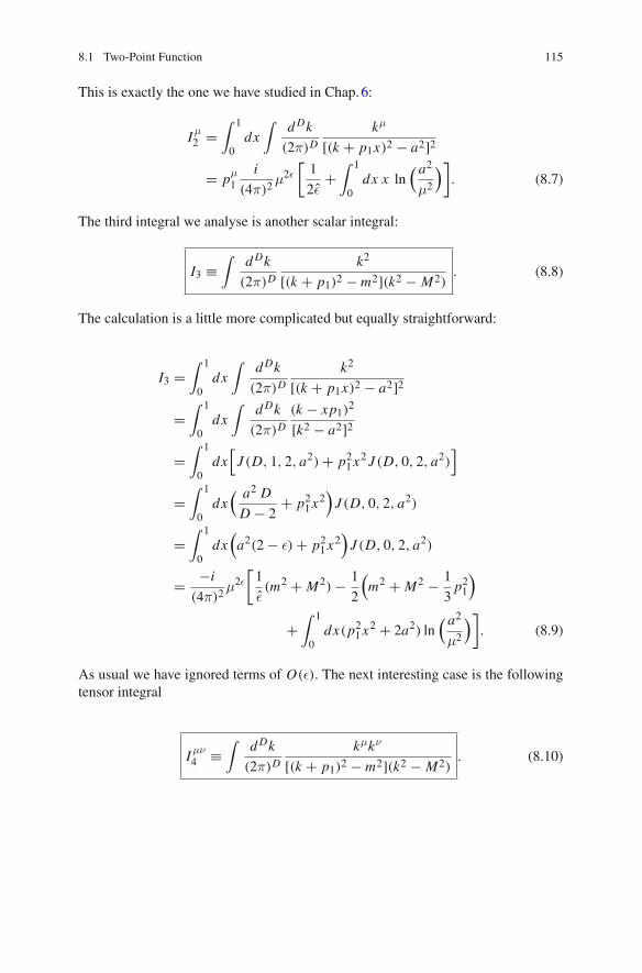
8.1 Two-Point Function 115

This is exactly the one we have studied in Chap. 6:

I μ2 =

∫ 1

0dx

∫d Dk

(2π)D

kμ

[(k + p1x)2 − a2]2

= pμ1

i

(4π)2μ2ε

[1

2ε+

∫ 1

0dx x ln

( a2

μ2

)]. (8.7)

The third integral we analyse is another scalar integral:

I3 ≡∫

d Dk

(2π)D

k2

[(k + p1)2 − m2](k2 − M2). (8.8)

The calculation is a little more complicated but equally straightforward:

I3 =∫ 1

0dx

∫d Dk

(2π)D

k2

[(k + p1x)2 − a2]2

=∫ 1

0dx

∫d Dk

(2π)D

(k − xp1)2

[k2 − a2]2

=∫ 1

0dx

[J (D, 1, 2, a2) + p21x2 J (D, 0, 2, a2)

]

=∫ 1

0dx

( a2 D

D − 2+ p21x2

)J (D, 0, 2, a2)

=∫ 1

0dx

(a2(2 − ε) + p21x2

)J (D, 0, 2, a2)

= −i

(4π)2μ2ε

[1

ε(m2 + M2) − 1

2

(m2 + M2 − 1

3p21

)

+∫ 1

0dx(p21x2 + 2a2) ln

( a2

μ2

)]. (8.9)

As usual we have ignored terms of O(ε). The next interesting case is the followingtensor integral

I μν4 ≡

∫d Dk

(2π)D

kμkν

[(k + p1)2 − m2](k2 − M2). (8.10)

116 8 One-Loop Two and Three-Point Functions

We find the following expression for I μν4 :

I μν4 =

∫ 1

0dx

∫d Dk

(2π)D

kμkν

[(k + p1x)2 − a2]2

=∫ 1

0dx

∫d Dk

(2π)D

(kμ − xpμ1 )(kν − xpν

1 )

[k2 − a2]2

=∫ 1

0dx

(gμν

D

a2D

D − 2+ pμ

1 pν1 x2

)J (D, 0, 2, a2)

= −i

(4π)2μ2ε

[(gμν

4(m2 + M2 − 1

3p21) + 1

3pμ1 pν

1

)1ε

− gμν

4

(m2 + M2 − 1

3p21

)

+∫ 1

0dx

(gμν

2a2 + pμ

1 pν1 x2

)ln

( a2

μ2

)]. (8.11)

The next integral we study is again a scalar type integral:

I5 ≡∫

d Dk

(2π)D

(k2)2

[(k + p1)2 − m2](k2 − M2). (8.12)

We obtain:

I5 =∫ 1

0dx

∫d Dk

(2π)D

(k2)2

[(k + p1x)2 − a2]2

=∫ 1

0dx

∫d Dk

(2π)D

2x2 p21k2 + 4

Dx2 p21k2 + (k2)2 + x4(p21)

2

[k2 − a2]2

=∫ 1

0dx

[(2x2 p21 + 4

Dx2 p21

) a2D

D − 2+ a4(D + 2)

D − 2+ x4(p21)

2]

J (D, 0, 2, a2)

= −i

(4π)2μ2ε

[1

ε

(m2(p21 + M2) + m4 + M4

)

+ 2

3

( (p21)2

5− m2(p21 + M2) − m4 − M4

)

+∫ 1

0dx

(3a4 + 6a2x2 p21 + x4(p21)

2)ln

( a2

μ2

)]. (8.13)

The last integral that we are going to analyse is

I μ6 ≡

∫d Dk

(2π)D

kμk2

[(k + p1)2 − m2](k2 − M2). (8.14)

8.1 Two-Point Function 117

Fig. 8.2 One-loop fermionictwo-point function in QED

i Σ(/p) =

p

k

p + k

We obtain the following:

I μ6 =

∫ 1

0dx

∫d Dk

(2π)D

kμk2

[(k + p1x)2 − a2]2

= −pμ1

∫ 1

0dx

[x(1 + 2

D

) a2D

D − 2+ x3 p21

]J (D, 0, 2, a2)

= pμ1

i

(4π)2μ2ε

∫ 1

0dx

[1

ε

(3a2x + x3 p21

)− 2a2x +

(3a2x + x3 p21

)ln

( a2

μ2

)]

= pμ1

i

(4π)2μ2ε

[1

ε

(m2 + M2

2

)+ 1

3

( p212

− 2m2 − M2)

+∫ 1

0dx

(3a2x + x3 p21

)ln

( a2

μ2

)]. (8.15)

In the same fashion, one should find straightforward to calculate any one-loopintegral for any arbitrary tensor function in the numerator. Next we will analyse atwo-point function that presents both IR and UV poles.

8.2 IR Divergences and the Two-Point Function

Besides the ultraviolet divergences we have seen until now, which are treated consis-tently within the renormalization procedure there are also other types of divergencescalled infrared, as we have seen in Chap.6. Consider the one-loop fermionic QEDtwo-point function for massless on-shell fermions in the Feynman gauge ξ = 1(Fig. 8.2). It reads1:

iΣ(/p) = −e2∫

d Dk

(2π)D

γμ(/p + /k)γμ

k2(k + p)2, (8.16)

1The QED Feynman rules are given in Chap.5.

118 8 One-Loop Two and Three-Point Functions

with p2 → 0 and where we have taken Q2 = 1 for the electric charge. Taking aquick look at the denominator we find that for small k

1

k2(k2 + 2p · k)

k2�−−→ 1

k2(2p · k). (8.17)

We know that denominator diverges in two cases:

1. k → 0, soft divergence,

2. p · k → 0, collinear divergence. (8.18)

It is worth mentioning that a typical way of regulating these divergences is by giv-ing small masses mγ, me both to the photon and the electron and taking the limitmγ, me → 0 at the end. However, the most elegant way is still, Dimensional Regu-larization (doesn’t break the symmetries of our theory). As seen in Chap.6, we musttake D = 4+ 2ε′, with ε′ > 0 for the IR divergent parts and D = 4+ 2ε, with ε < 0for the UV divergent parts. In D dimensions the two-point function (8.16) reads:

iΣ(/p) = −e2∫

d Dk

(2π)D

(2 − D)(/p + /k)

k2(k + p)2

= −e2∫ 1

0dx

∫d Dk

(2π)D

(2 − D)(/p + /k)

[(k + xp)2 − a2]2

= −e2(2 − D)/p∫ 1

0dx(1 − x)J (D, 0, 2, a2). (8.19)

where we have defined a2 ≡ −p2x(1 − x). Now, instead of writing J (D, 0, 2, a2)

as (6.9), let’s write it in the form of (6.2):

iΣ(/p) = −i

(4π)D/2 /pe2(2 − D)Γ (2 − D/2)∫ 1

0dx(1 − x)(a2)D/2−2

= −i

(4π)D/2 /pe2(2 − D)Γ (2 − D/2)(−p2)D/2−2

×∫ 1

0dx(1 − x)D/2−1x D/2−2. (8.20)

Using the Euler Beta function (A.17) we find the following:

iΣ(/p) = −i

(4π)D/2 /pe2(2 − D)Γ (2 − D/2)Γ (D/2)Γ (D/2 − 1)

Γ (D − 1)(−p2)D/2−2.

(8.21)

We have an UV pole at D = 4 coming from Γ (2− D/2) and we have an indetermi-nation of the type 00 for (−p2)D/2−2 when p2 → 0 and D → 4, which will appear

8.2 IR Divergences and the Two-Point Function 119

in our equations in the form of IR and UV poles. In order to regularize this, we mustuse the following integral:

∫ ∞

−y

dx

xxε = (−y)ε

(− 1

ε

). (8.22)

Therefore, (−p2)D/2−2 can be written in the following form

(−p2)D/2−2 = (2 − D/2)∫ ∞

−p2

dq2

q2 (q2)D/2−2

= (2 − D/2)(μ2)D/2−2∫ ∞

−p2

dq2

q2

(q2

μ2

)D/2−2

= (2 − D/2)(μ2)D/2−2[ ∫ μ2

−p2

dq2

q2

(q2

μ2

)D/2−2

+∫ ∞

μ2

dq2

q2

(q2

μ2

)D/2−2]. (8.23)

In order to make these integrations we need the following intermediate results

∫ μ

0dx

1

x

( x

μ

)ε = 1

εfor Re(ε) > 0 and μ > 0

∫ ∞

μdx

1

x

( x

μ

)ε = −1

εfor Re(ε) < 0 and μ > 0 (8.24)

Therefore, we can safely take p2 → 0 in (8.23) and we obtain

(−p2)D/2−2 = (2 − D/2)(μ2)D/2−2[ 1ε′ − 1

ε

]. (8.25)

Taking D adequately in each case we find

iΣ(/p) = −i

(4π)2/pe2

[−

(μ2

4π

)ε′( 1

ε′ + γE

)+

(μ2

4π

)ε(1ε

+ γE

)], (8.26)

where we have summed and subtracted γE and we have ignored all terms of O(ε)and O(ε′). Introducing our standard notation for the UV pole (6.7) and making asimilar definition for the IR pole

1

ε′ ≡ 1

ε′ + γE − ln(4π) , (8.27)

120 8 One-Loop Two and Three-Point Functions

we finally obtain

iΣ(/p) = −i /pα

4π

[− μ2ε′

( 1

ε′)

+ μ2ε(1

ε

)]. (8.28)

The usual renormalization approach is to also absorb the IR pole into the renor-malization constant. Therefore we have Z1 = Z2 = 1 + δ1 = 1 + δ2 (rememberZ1 = Z2, see Chap.7) with

δ1 = δ2 = α

4π

[− μ2ε′

( 1

ε′)

+ μ2ε(1

ε

)], (8.29)

for the M S-scheme. Note that the renormalized self-energy ΣR(/p) = 0 in this case.One should also realize that Z1 and Z2 do not contribute to the renormalization ofany physical quantity like the electric charge or the mass and therefore, the running(with the renormalization scale) of the these physical quantities is not affected by theIR pole we have included in δ1,2 (as it must, the running of physical quantities onlydepends on the UV-poles and never on the IR-poles). This last result, (8.29) will turnout to be extremely useful within a few sections, where we will analyse an exampleof IR-pole cancellation.

Next, we shall move on and analyse the three-point functions. The IR divergencesthat will appear will be much easier to localize and to treat.

8.3 Three-Point Function

Momentum conservation in this case reads

p1 = p2 + p3, (8.30)

and as usual, the exterior legs are not necessarily on-shell. The arrows in Fig. 8.3indicate the distribution ofmomenta, and all themasses are considered to be different.The denominator of this three-point function is:

1

(k2 − M2)[(k + p2)2 − m2][(k − p3)2 − m2] . (8.31)

The Feynman parametrization that we shall use in this case is (6.25). Taking A =(k2 − M2), B = [(k + p2)2 − m2] and C = [(k − p3)2 − m2] we obtain:

1

(k2 − M2)[(k + p2)2 − m2][(k − p3)2 − m2] =∫ 1

0dy

∫ 1−y

0dz

2

D3 . (8.32)

8.3 Three-Point Function 121

p1, m1

p2, m2

p3, m3

k, M

k + p2, m

k − −p3, m

Fig. 8.3 Distribution of masses and momenta of the three-point function

with D given by:

D = (k + p2y − p3z)2 − b2, (8.33)

b2 = m2y + m2z + M2(1 − y − z) + p23z(z − 1)

+ p22 y(y − 1) − 2yz(p2 · p3). (8.34)

The first integral that we shall deal with is the scalar integral:

C1 ≡∫

d Dk

(2π)D

1

(k2 − M2)[(k + p2)2 − m2][(k − p3)2 − m2] . (8.35)

Introducing the Feynman parametrization and manipulating the expression:

C1 =∫ 1

0dy

∫ 1−y

0dz

∫d Dk

(2π)D

2

[(k + p2y − p3z)2 − b2]3

=∫ 1

0dy

∫ 1−y

0dz

∫d Dk

(2π)D

2

[k2 − b2]3

= 2∫ 1

0dy

∫ 1−y

0dz J (D, 0, 3, b2)

= −i

(4π)2

∫ 1

0dy

∫ 1−y

0dz

1

b2. (8.36)

The second integral we wish to calculate is the vector integral:

Cμ2 ≡

∫d Dk

(2π)D

kμ

(k2 − M2)[(k + p2)2 − m2][(k − p3)2 − m2] . (8.37)

122 8 One-Loop Two and Three-Point Functions

Introducing the Feynman parametrization we obtain:

Cμ2 =

∫ 1

0dy

∫ 1−y

0dz

∫d Dk

(2π)D

2kμ

[(k + p2y − p3z)2 − b2]3

= 2∫ 1

0dy

∫ 1−y

0dz(−pμ

2 y + pμ3 z)J (D, 0, 3, b2)

= −i

(4π)2

∫ 1

0dy

∫ 1−y

0dz

−pμ2 y + pμ

3 z

b2. (8.38)

The next integral we are going to calculate is:

C3 ≡∫

d Dk

(2π)D

k2

(k2 − M2)[(k + p2)2 − m2][(k − p3)2 − m2] . (8.39)

Manipulating the expression we get:

C3 =∫ 1

0dy

∫ 1−y

0dz

∫d Dk

(2π)D

2k2

[(k + p2y − p3z)2 − b2]3

= 2∫ 1

0dy

∫ 1−y

0dz

[(1 + ε

2

)J (D, 0, 2, b2) + (

p2y − p3z)2

J (D, 0, 3, b2)

]

= −i

(4π)2μ2ε

∫ 1

0dy

∫ 1−y

0dz

[2

ε+ 2 ln

( b2

μ2

)+ 1 + 1

b2(

p2y − p3z)2

]

= −i

(4π)2μ2ε

{1

ε+ 1

2+

∫ 1

0dy

∫ 1−y

0dz

[(p2y − p3z

)2

b2+ 2 ln

( b2

μ2

)]}.

(8.40)

The last integral that we will analyse in this section is tensor integral Cμν4 :

Cμν4 ≡

∫d Dk

(2π)D

kμkν

(k2 − M2)[(k + p2)2 − m2][(k − p3)2 − m2] . (8.41)

We obtain the following result:

Cμν4 =

∫ 1

0dy

∫ 1−y

0dz

∫d Dk

(2π)D

2kμkν

[(k + p2y − p3z)2 − b2]3

= 2∫ 1

0dy

∫ 1−y

0dz

[gμν

4J (D, 0, 2, b2)

+ (ypμ

2 − zpμ3

)(ypν

2 − zpν3

)J (D, 0, 3, b2)

]

8.3 Three-Point Function 123

= −i

(4π)2μ2ε

{gμν 1

4ε+

∫ 1

0dy

∫ 1−y

0dz

×[1

b2(ypμ

2 − zpμ3

)(ypν

2 − zpν3

) + 1

2gμν ln

( b2

μ2

)]}. (8.42)

For a generic N-point function one can use the Feynman parametrization (6.27)introduced previously in Chap.6.

We will now move on to the analysis of the IR divergences of the three-pointfunctions we have studied in this section.

8.4 IR Divergences and the Three-Point Function

Consider the following configuration for the previously introduced three point func-tions

p22 = m22 = m2, p23 = m2

3 = m2, M2 = 0. (8.43)

with m2i �= 0 or m2

i = 0. In this case the denominator we have is:

1

k2(k2 + 2p2 · k)(k2 − 2p3 · k)

k2�−−→ 1

k2(2p2 · k)(2p3 · k), (8.44)

with the two usual infrared divergences:

1. k → 0, soft divergence,

2. p3 · k or p2 · k → 0, collinear divergence. (8.45)

Here we shall only consider the most simple case for massless on-shell particlesm2

i = 0. The case with m2i �= 0 is left for the reader as an exercise. For these

calculations we shall switch to Feynman parametrisation (6.24). Choosing A =k2 + 2p2 · k, B = k2 − 2p3 · k and C = k2 as in (6.34), we obtain:

1

ABC=

∫ 1

0dx

∫ 1

0dy

2x

D3 , (8.46)

with the denominator D given by

D =(

k + p2xy − p3x(1 − y))2 − b2, (8.47)

b2 = −2(p2 · p3)x2y(1 − y). (8.48)

As we have seen in Chap.6, we can not take D → 4 in J (D, 0, 3, b2) when IRdivergences are present. The expression we will be needing is:

124 8 One-Loop Two and Three-Point Functions

J (D, 0, 3, b2) = −i

(4π)D/2

1

2Γ (3 − D/2)(b2)D/2−3 , (8.49)

which we have already introduced in (6.35).The three point functions treated in this section will carry an IR sub-index. The

first scalar three-point function that we have is (6.31). For completeness we shallpresent parts of this the calculation again:

C1,IR = 2∫ 1

0dx

∫ 1

0dyx J (D, 0, 3, b2)

= −i

(4π)D/2Γ (3 − D/2)∫ 1

0dx

∫ 1

0dyx(b2)D/2−3

= −i

(4π)D/2Γ (3 − D/2)(−2p2 · p3)D/2−3

∫ 1

0dxx D−5

×∫ 1

0dyyD/2−3(1 − y)D/2−3

= −i

(4π)D/2

Γ (3 − D/2)

Γ (D − 3)(−2p2 · p3)

D/2−3Γ (D/2 − 2)Γ (D/2 − 2).

(8.50)

Taking D adequately we get the following result:

C1,IR =∫

d Dk

(2π)D

1

k2(k + p2)2(k − p3)2

= i

(4π)2

1

2p2 · p3

(−2p2 · p34π

)ε′ Γ (1 − ε′)Γ (1 + 2ε′)

Γ 2(ε′) (8.51)

Let’s now continue and analyse the second integral Cμ2,IR:

Cμ2,IR = 2

∫ 1

0dx

∫ 1

0dyx

(− pμ

2 xy + pμ3 x(1 − y)

)J (D, 0, 3, b2)

= −i

(4π)D/2

Γ (3 − D/2)Γ (D − 3)

Γ (D − 2)(−2p2 · p3)

D/2−3

×∫ 1

0dy

(− pμ

2 y + pμ3 (1 − y)

)(y(1 − y)

)D/2−3

= −i

(4π)D/2

Γ (3 − D/2)Γ (D − 3)

Γ (D − 2)(−2p2 · p3)

D/2−3

× (pμ3 − pμ

2 )Γ (D/2 − 1)Γ (D/2 − 2)

Γ (D − 3). (8.52)

8.4 IR Divergences and the Three-Point Function 125

We obtain the following simple result:

Cμ2,IR =

∫d Dk

(2π)D

kμ

k2(k + p2)2(k − p3)2

= (pμ3 − pμ

2 )i

(4π)2

1

2p2 · p3

×(−2p2 · p3

4π

)ε′ Γ (1 − ε′)Γ (1 + ε′)Γ (2 + 2ε′)

Γ (ε′) (8.53)

Continuing with the third integral we get:

C3,IR =∫ 1

0dx

∫ 1

0dy

∫d Dk

(2π)D

2xk2

[(k + p2xy − p3x(1 − y))2 − b2]3

=∫ 1

0dx

∫ 1

0dy

( x

2D J (D, 0, 2, b2) − 4(p2 · p3)x3y(1 − y)J (D, 0, 3, b2)

)

≡ B(J (D, 0, 2, b2)

) + C(J (D, 0, 3, b2)

). (8.54)

The B function is, of course, UV divergent:

B =∫ 1

0dx

∫ 1

0dy

x

2D J (D, 0, 2, b2)

= −i

(4π)2μ2ε

[1ε

+ 1

2+ 2

∫ 1

0dx

∫ 1

0dyx ln

( b2

μ2

)]

= −i

(4π)2μ2ε

[1ε

+ 1

2+ ln

(−2p2 · p3μ2

)+ 2

∫ 1

0dx

∫ 1

0dyx ln[x2y(1 − y)]

]

= −i

(4π)2μ2ε

[1ε

− 5

2+ ln

(2p2 · p3μ2

)± iπ

], (8.55)

where we have taken

ln(−1) = ln e±iπ = ±iπ. (8.56)

The second integral, as we shall see is in fact, finite:

C = −4(p2 · p3)∫ 1

0dx

∫ 1

0dyx3y(1 − y)J (D, 0, 3, b2)

= 2(p2 · p3)i

(4π)D/2Γ (3 − D/2)∫ 1

0dx

∫ 1

0dy x3y(1 − y)(b2)D/2−3. (8.57)

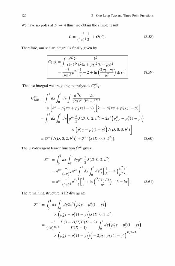
126 8 One-Loop Two and Three-Point Functions

We have no poles at D → 4 thus, we obtain the simple result

C = −i

(4π)2

1

2+ O(ε′). (8.58)

Therefore, our scalar integral is finally given by

C3,IR =∫

d Dk

(2π)D

k2

k2(k + p2)2(k − p3)2

= −i

(4π)2μ2ε

[1ε

− 2 + ln(2p2 · p3

μ2

)± iπ

](8.59)

The last integral we are going to analyse is Cμν4,IR:

Cμν4,IR =

∫ 1

0dx

∫ 1

0dy

∫d Dk

(2π)D

2x

[k2 − b2]3×

[kμ − pμ

2 xy + pμ3 x(1 − y)

][kν − pν

2 xy + pν3 x(1 − y)

]

=∫ 1

0dx

∫ 1

0dy

[gμν x

2J (D, 0, 2, b2) + 2x3

(pμ2 y − pμ

3 (1 − y))

×(

pν2 y − pν

3 (1 − y))

J (D, 0, 3, b2)

]

≡ Eμν(J (D, 0, 2, b2)

) + Fμν(J (D, 0, 3, b2)

). (8.60)

The UV-divergent tensor function Eμν gives:

Eμν =∫ 1

0dx

∫ 1

0dygμν x

2J (D, 0, 2, b2)

= gμν −i

(4π)2μ2ε

∫ 1

0dx

∫ 1

0dy

x

2

[1ε

+ ln( b2

μ2

)]

= gμν −i

(4π)2μ2ε 1

4

[1ε

+ ln(2p2 · p3

μ2

)− 3 ± iπ

]. (8.61)

The remaining structure is IR divergent:

Fμν =∫ 1

0dx

∫ 1

0dy2x3

(pμ2 y − pμ

3 (1 − y))

×(

pν2 y − pν

3 (1 − y))

J (D, 0, 3, b2)

= −i

(4π)D/2

Γ (3 − D/2)Γ (D − 2)

Γ (D − 1)

∫ 1

0dy

(pμ2 y − pμ

3 (1 − y))

×(

pν2 y − pν

3 (1 − y))(

− 2p2 · p3y(1 − y))D/2−3

8.4 IR Divergences and the Three-Point Function 127

= −i

(4π)D/2

Γ (3 − D/2)Γ (D − 2)

Γ (D − 1)(−2p2 · p3)

D/2−3

×[(pμ

2 pν2 + pμ

3 pν3 )

Γ (D/2)Γ (D/2 − 2)

Γ (D − 2)

− (pμ2 pν

3 + pν2 pμ

3 )Γ (D/2 − 1)Γ (D/2 − 1)

Γ (D − 2)

]. (8.62)

Therefore, the final expression for Cμν4,IR that we find is:

Cμν4,IR =

∫d Dk

(2π)D

kμkν

k2(k + p2)2(k − p3)2

= gμν −i

(4π)2μ2ε 1

4

[1ε

+ ln(2p2 · p3

μ2

)− 3 ± iπ

]

+ i

(4π)2

1

2p2 · p3

(−2p2 · p34π

)ε′ Γ (1 − ε′)Γ (3 + 2ε′)

×[(pμ

2 pν2 + pμ

3 pν3 )Γ (2 + ε′)Γ (ε′)

− (pμ2 pν

3 + pν2 pμ

3 )Γ 2(1 + ε′)]

(8.63)

In the followingwe shall introduce the twoand three-bodyphase space expressionsin D = 4+2ε′ dimensions, needed for the calculation of IR-divergent cross sections.Afterwards, we will calculate an IR divergent process for which we will make useof all the IR-divergent integrals introduced in this section and also the IR-divergenttwo-point function presented previously.

8.5 Two and Three-Body Phase Space in D Dimensions

For D = 4 + 2ε′ with ε′ > 0 we have the following two-body phase space:

∫d Q2 = 1

4π

p√s

( p2

π

)ε′ 1

Γ (1 + ε′)

∫ 1

0dv[v(1 − v)]ε′ (8.64)

where p ≡ |p| = γm|v| is the center of mass momentum (of the final state particles)given by

p = 1

2√

sλ1/2(s, m2

a, m2b), (8.65)

128 8 One-Loop Two and Three-Point Functions

and where λ(x, y, z) is the usual Kallen function λ(x, y, x) ≡ x2 + y2 + z2 −2xy −2yz − 2xz. The variable v is defined as

v = 1 + cos θ

2, (8.66)

with θ the CM scattering angle. If we are dealing with final state identical particles,we need to also multiply by the 1/2 symmetry factor. If the squared transition matrixdoes not depend on the angle θ, we can integrate over v and obtain the simple result

∫d Q2 = 1

4π

p√s

( p2

π

)ε′ Γ (1 + ε′)Γ (2 + 2ε′)

. (8.67)

The three-body phase space is given by:

∫dQ3 =

Q2

2(4π)3( 4π

Q2

)−2ε′ 1Γ (2 + 2ε′)

∫ 1

0dx1

∫ 1

1−x1

dx2

× [(1 − x1)(1 − x2)(1 − x3)

]ε′

(8.68)

where Qμ = pμ1 + pμ

2 + pμ3 (with pμ

i the final state particle momenta) and wherewe have introduced the xi kinematical variables:

x1 ≡ 2(p1 · Q)

Q2 , x2 ≡ 2(p2 · Q)

Q2 , x3 ≡ 2(p3 · Q)

Q2 . (8.69)

It is easy to check that x1 + x2 + x3 = 2. If we have n final state identical particles

(n = 2, 3) we must also multiply by the1

n! symmetry factor.

When averaging over the spins of the initial state particles, it is conventional toconsider for massless on-shell photons or gluons D − 2 = 2(1 + ε′) polarizations.Fermions are considered to have two spin-polarization states as usual.

8.6 Cancellation of IR Divergences

Consider the following collision f f → γ∗ → e+e−γ, with f f any fermion-antifermion pair. The corresponding cross-section for this process can be written as

σ ∼ Fμν∫

d Q3 Lμν, (8.70)

8.6 Cancellation of IR Divergences 129

with Fμν the initial state fermionic tensor and with Lμν the final state leptonic tensor.Due toQED gauge invariance we canwrite the previous expression (8.70) in the form

σ ∼ Fαβ gαβ

∫d Q3 Lμν gμν, (8.71)

therefore, the calculation of this cross section can be broken into two disjoint pieces.As we are only interested in the final state (it is where the IR divergences will appear)we will just focus on the sub-process γ∗ → e+e−γ. Thus, for practical purposes wecan consider that the virtual photon γ∗ is described by some polarization vectors ε

μs

and, we can perform the usual substitution∑

s εμs εν∗

s → −gμν when calculating thesquared transition matrix.2 For this analysis we shall consider massless electrons. Atleading order there are two diagrams that contribute to our sub-process:

−i M =

e+

e−

γ∗ γ

+

e+

e−

γ

γ∗

(1) (2)

where the squared transitionmatrix |M|2 = |M1+M2|2 is ofO(e4).When calculat-ing the cross section corresponding to this process one finds that it has IR divergences.This is mainly due to the fact that, we can have soft or collinear emitted photons thatare experimentally indistinguishable from just a electron. Schematically:

orsoft collinear

∼

Roughly speaking, in the soft or collinear limit the three-body final state turns intoa two-body final state. Thus, in order to be able to remove the IR divergences wemust also analyse the 2 → 2 scattering process given by f f → γ∗ → e+ e− (withf f the same fermion-antifermion pair as in the previous case). The cross sectionfor this process can be separated exactly as in (8.71) (obviously with d Q2 insteadof d Q3) therefore we can, again, focus only on the sub-process γ∗ → e+ e−. Thetransition amplitude for this sub-process including one-loop corrections (seeChap. 7)it is given by:

+ +−i M′ = δ1

(1) (2)

2As the photon is not a real (on-shell) particle we shall not average over its polarizations whencalculating the cross section.

130 8 One-Loop Two and Three-Point Functions

The matrix element can, thus, be written as M′ = M′1 + M′

2 + δ1M′1 with the

amplitude M′1 of O(e) and with the amplitudes M′

2 and δ1M′1 of O(e3). As we

already know δ1 is an IR divergent quantity and, as we can suspect, it will also be thecase for the amplitude M′

2. It turns out that summing to the cross section of the firstprocess σ(γ∗ → e+e−γ), the part of σ(γ∗ → e+e−) that contributes to the sameorder in perturbation theory, that is O(e4), the IR poles cancel. We can thereforedefine a proper infrared safe (IRS) observable given by3

σIRS(γ∗ → e+e−γ) = σ(γ∗ → e+e−γ) + σ(γ∗ → e+e−)

= 1

2s

( ∫d Q3

∑

ri

|M|2 +∫

d Q2

∑

ri

∣∣M′∣∣2)

(8.72)

where∑

ristands for the sum over the initial and final state particle polarizations and

where∣∣M′∣∣2 is defined as the part of the squared amplitude

∣∣M′∣∣2, that contributesto the cross section at O(e4). Its explicit expression is given by

∣∣M′∣∣2 ≡ 2Re[M′†1M′

2] + 2δ1|M′1|2 , (8.73)

Let’s thus, start by calculating the first process:

e+

e−

γ∗(p1) γ+

e+

e−

γ

γ∗(p1)

p2

p2 + p4

p3

p2

p3 + p4

p3

p4 p4

The squared matrix element is given by |M|2 = |M1 +M2|2 = |M1|2 +|M2|2 +2Re[M†

1M2]. In D dimensions we obtain the following results:

∑

ri

|M1|2 = e4

4(p2 · p4)2Tr{γν( /p2 + /p4)γ

μ/p3γμ( /p2 + /p4)γν /p2}

= 2e4

(p2 · p4)(D − 2)2(p3 · p4) (8.74)

3Read Chap.3 for Relativistic kinematics, phase space and cross section formulae, and Chap.5 formore details on calculations of QED processes and the corresponding Feynman rules.

8.6 Cancellation of IR Divergences 131

∑

ri

|M2|2 = e4

4(p3 · p4)2Tr{γμ( /p3 + /p4)γ

ν/p3γν( /p3 + /p4)γμ /p2}

= 2e4

(p3 · p4)(D − 2)2(p2 · p4) (8.75)

The crossed term reads:

∑

ri

2Re[M†1M2] = − e4

4(p2 · p4)(p3 · p4)

× Tr{γν( /p2 + /p4)γμ

/p3γν( /p3 + /p4)γμ /p2}

= 4e4

(p3 · p4)(p2 · p4)(D − 2)

×[(D − 4)(p2 · p4)(p3 · p4)

+ 2(p2 · p3)2 + 2(p2 · p4)(p2 · p3)

+ 2(p3 · p4)(p2 · p3)]

(8.76)

The minus sign (from the RHS of the first line of the previous expression) is due tothe fermionic propagator of the first diagram (which goes in the opposite directionof the momentum, and therefore it has the form −i( /p2 + /p4)/(2p2 · p4) and noti( /p2 + /p4)/(2p2 · p4)). Introducing the xi kinematical variables from the previoussection

x1 ≡ 2(p2 · Q)

Q2 , x2 ≡ 2(p3 · Q)

Q2 , x3 ≡ 2(p4 · Q)

Q2 , (8.77)

with Q ≡ p1 = p2 + p3 + p4 (and where, remember, x1 + x2 + x3 = 2) we obtainthe following results:

(p2 · p4) = 1

2x1Q2 − (p2 · p3), (8.78)

(p3 · p4) = 1

2x2Q2 − (p2 · p3), (8.79)

(p2 · p3) = 1

2Q2(x1 + x2 − 1). (8.80)

Performing these substitutions, taking D = 4 + 2ε′ (with ε′ > 0) and keeping theterms up to O(ε′2) we obtain the following simple formula for the squared transitionmatrix

∑

ri

|M|2 = 8e4(ε′ + 1)x21 + x22 + ε′(x1 + x2 − 2)2

(1 − x1)(1 − x2). (8.81)

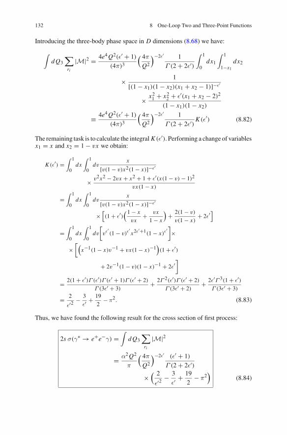
132 8 One-Loop Two and Three-Point Functions

Introducing the three-body phase space in D dimensions (8.68) we have:

∫d Q3

∑

ri

|M|2 = 4e4Q2(ε′ + 1)

(4π)3

( 4π

Q2

)−2ε′ 1

Γ (2 + 2ε′)

∫ 1

0dx1

∫ 1

1−x1dx2

× 1

[(1 − x1)(1 − x2)(x1 + x2 − 1)]−ε′

× x21 + x22 + ε′(x1 + x2 − 2)2

(1 − x1)(1 − x2)

≡ 4e4Q2(ε′ + 1)

(4π)3

( 4π

Q2

)−2ε′ 1

Γ (2 + 2ε′)K (ε′) (8.82)

The remaining task is to calculate the integral K (ε′). Performing a change of variablesx1 = x and x2 = 1 − vx we obtain:

K (ε′) =∫ 1

0dx

∫ 1

0dv

x

[v(1 − v)x2(1 − x)]−ε′

× v2x2 − 2vx + x2 + 1 + ε′(x(1 − v) − 1)2

vx(1 − x)

=∫ 1

0dx

∫ 1

0dv

x

[v(1 − v)x2(1 − x)]−ε′

×[(1 + ε′)

(1 − x

vx+ vx

1 − x

)+ 2(1 − v)

v(1 − x)+ 2ε′

]

=∫ 1

0dx

∫ 1

0dv

[vε′(1 − v)ε

′x2ε

′+1(1 − x)ε′]×

×[(

x−1(1 − x)v−1 + vx(1 − x)−1)(1 + ε′)

+ 2v−1(1 − v)(1 − x)−1 + 2ε′]

= 2(1 + ε′)Γ (ε′)Γ (ε′ + 1)Γ (ε′ + 2)

Γ (3ε′ + 3)+ 2Γ 2(ε′)Γ (ε′ + 2)

Γ (3ε′ + 2)+ 2ε′Γ 3(1 + ε′)

Γ (3ε′ + 3)

= 2

ε′2− 3

ε′ + 19

2− π2. (8.83)

Thus, we have found the following result for the cross section of first process:

2s σ(γ∗ → e+e−γ) =∫

d Q3

∑

ri

|M|2

= α2Q2

π

( 4π

Q2

)−2ε′ (ε′ + 1)

Γ (2 + 2ε′)

×( 2

ε′2 − 3

ε′ + 19

2− π2

)(8.84)

8.6 Cancellation of IR Divergences 133

We now move on, and calculate the remaining cross section σ(γ∗ → e+e−). Thefirst amplitude that contributes to this process is given by M′

1:

−i M′1 =

e+(p2)

e−(p3)

γ∗(p1)

M′1 = −eεr1

μ (p1)ur3(p3)γμvr2(p2). (8.85)

where we have taken the charge of the electron Q = −1 (do not confuse it with thefour-momentum Qμ). The second amplitude of the process, M′

2 is given by:

−i M′2 =

e+(p2)

e−(p3)

p3 − k

−k − p2

k

γ∗(p1)

M′2 = i e3εr1

μ (p1)ur3(p3)Γμvr2(p2), (8.86)

where Γ μ reads

Γ μ =∫

d Dk

(2π)D

γρ(/k − /p3)γμ(/k + /p2)γρ

k2(k + p2)2(k − p3)2. (8.87)

Working in D dimensions, and using the Dirac equations of motion for masslessfermions /p2vr2(p2) = 0 and ur3(p3) /p3 = 0 in order to eliminate some of the terms,we find

Γ μ =∫

d Dk

(2π)D

(4 − 2D)kμ/k + (D − 2)γμk2 + 2/kγμ/p3 − 2 /p2γμ/k + 2 /p2γμ

/p3k2(k + p2)2(k − p3)2

= (4 − 2D)γνCμν4,IR + (D − 2)γμC3,IR

+ 2(γνγμ

/p3 − /p2γμγν)C

ν2,IR + 2 /p2γ

μ/p3C1,IR

= Aγμ + B /p2γμ

/p3. (8.88)

134 8 One-Loop Two and Three-Point Functions

The coefficients A and B are given by

A = −i

(4π)2μ2ε

[1ε

+ ln(2p2 · p3

μ2

)± iπ

],

B = i

(4π)2

1

2p2 · p3

(−2p2 · p34π

)ε′[2

Γ (1 − ε′)Γ (1 + 2ε′)

Γ 2(ε′)

− 4Γ (1 − ε′)Γ (1 + ε′)

Γ (2 + 2ε′)Γ (ε′)

], (8.89)

where again, we have used the equations of motion to eliminate terms. The lastamplitude is simply −iδ1M′

1 with δ1 given by (8.29). We obtain

δ1M′1 = ie3εr1

μ (p1)ur3(p3)Γμvr2(p2), (8.90)

where we have defined Γ μ as

Γ μ = γμ i

(4π)2

[− μ2ε′

( 1

ε′)

+ μ2ε(1

ε

)]. (8.91)

We can now proceed with our calculation of |M′∣∣2 using (8.73) or equivalently, wecan define the UV-finite (but IR-divergent) amplitude M′ R

2 = M′2 + δ1M′

1 thus,

|M′∣∣2 = 2Re [M′†1M′ R

2 ]. Using this last approach, we find

M′ R2 = i e3εr1

μ (p1)ur3(p3)ΓμR vr2(p2), (8.92)

with ΓμR = Γ μ + Γ μ = ARγμ + B /p2γμ

/p3, and where

AR = −i

(4π)2

[μ2ε′ 1

ε′ + ln(2p2 · p3

μ2

)± iπ

]

= −i

(4π)2

[ 1ε′ + γE − ln(4π) + ln(2p2 · p3) ± iπ

]+ O(ε′). (8.93)

Using the expansion

ln(2p2 · p3

4π

)= 1

ε′

[ (2p2 · p34π

)ε′ − 1

]+ O(ε′), (8.94)

the final expression of AR reads

AR = −i

(4π)2

[1

ε′(2p2 · p3

4π

)ε′ + γE ± iπ]. (8.95)

8.6 Cancellation of IR Divergences 135

The squared amplitude is finally given by:

∑

ri

|M′∣∣2 = 2Re[i e4 Tr

{γμ /p3 (γμ AR + B /p2γ

μ/p3) /p2

}]

= 8 α2 Q2( Q2

4π

)ε′(1 + ε′)

×[Re

((−1)ε

′)(− 2

Γ (1 − ε′)Γ (1 + 2ε′)

Γ 2(ε′)

+ 4Γ (1 − ε′)Γ (1 + ε′)

Γ (2 + 2ε′)Γ (ε′)

)− 1

ε′ − γE

](8.96)

where Q2 = p21 = 2p2 · p3. As the squared transition matrix does not dependon the angle θ we can directly introduce the expression (8.67) for the phase space.Expanding in ε′ we obtain the needed cross section:

2s σ(γ∗ → e+e−) =∫

d Q2

∑

ri

|M′|2

= α2Q2

π

( 4π

Q2

)−2ε′ (1 + ε′)Γ (2 + 2ε′)

(− 2

ε′2 + 3

ε′ − 8 + π2)

(8.97)

Thus, as we mentioned, the poles from the two processes cancel, and the sum is finite

σIRS(γ∗ → e+e−γ) = 3α2

4π. (8.98)

When studying examples of IR divergences cancellation, the typical process thatone finds is e+e− → hadrons. At leading order the cross section for this process issimply given by σ(e+e− → qq) ≡ σ0 where qq stands for a quark-antiquark pair.At next-to-leading order one simply adds a gluon attached to the final state quarksσ(e+e− → qqg) ≡ σ1. This last process is of course IR divergent (due to radiationof soft or collinear gluons). By calculating the QCD vertex correction for the firstprocess (e+e− → qq), with a virtual gluon attached to the final state quarks, againone finds IR divergences. As seen in the previous example, the IR divergences fromthe vertex correction of σ0 and the ones from σ1 cancel and one finds

σ(e+e− → hadrons) = σ0

(1 + 3α2

s

4πCF + . . .

). (8.99)

withαs the strongQCDcoupling andCF = 4/3 the SU (3) invariant. The calculationfor this process is exactly the same as the one we just did, except we have made a

136 8 One-Loop Two and Three-Point Functions

Fig. 8.4 Two-loop diagramthat contributes to theanomalous magneticmoment of the muon

γ

h

G±

W±W±

μ− νμ μ−

few simplifications. We have considered photons instead of gluons in the final state(thus, we got rid of the colour factors), we have ignored the initial state collision,and we have also ignored the tree-level process (given by σ0).

8.7 Introduction to Two-Loops

Two-loop calculations are a highly advanced topic and one small subsection is obvi-ously not able to cover it. However we just want to provide the reader with one lastcomputational tool. As we have mentioned at the beginning of this chapter, we shallexplain with a very simple two-loop example how the generic Feynman parametriza-tion (6.27) can be used for non-integer powers of propagators.

Imagine we want to calculate the contribution from Fig. 8.4 to the anomalousmagnetic moment of the muon (or electron), where G± is the charged Goldstoneboson, W ± the charged gauge boson, and h the Higgs boson of the StandardModel.4

This is a quite simple topology and can be broken into twoparts.Wewill first calculatethe γW W effective vertex (which will, fortunately, turn out to be finite) and we willuse the expression of this vertex to calculate the second loop. Diagrammaticallythis is shown in Fig. 8.5, where Q = −1 is the electric charge of the muon. Theamplitude of this process has the form M ∼ εs

μ Γ μ (with εsμ the polarization vector

of the photon) thus all terms proportional to qμ will not contribute. The structure ofthe Γ μ vertex can therefore be written as

ur (p + q) Γ μ ur ′(p) = ur (p + q)[γμF1(q

2) + i

2mσμνqν F2(q

2)

+ γ5i

2mσμνqν F3(q

2) + . . .]

ur ′(p). (8.100)

4For a complete set of Feynman rules for the Standard Model read J. C. Romao and J. P. Silva, Aresource for signs and Feynman diagrams of the Standard Model, Int. J. Mod. Phys. A 27 (2012)1230025, http://arxiv.org/pdf/1209.6213.pdf..

8.7 Introduction to Two-Loops 137

i Γ ρμν ≡

γ

h

G+

W+

W+ ρμ

νk′

q

k′ − q

k − q

k − k′

−i e Q Γ μ ≡μ− νμ μ−

γ

k′ − qk′

q

p p + k p + q

μ

ν

ν ′

ρ

ρ′

W+W+

iΓρμν

Fig. 8.5 One-loop γW W effective vertex and its insertion into the second loop

with Fi (q2) scalar form factors and wherem is the mass of the muon. The anomalousmagnetic moment of the muon, denoted as Δaμ, is given by the F2(q2) form factorfor an on-shell photon i.e., Δaμ = F2(q2 = 0). Using the standard Feynman rulesfor the electro-weak SM Lagrangian, working in the linear Rξ gauge with ξW = 1(thus MG± = MW ), one finds (the needed Feynman rules for this calculation aregiven in Fig. 8.6)

i Γ ρμν = −ie

(4π)2

M2W

v2gμν(k′ρ − qρ) μ2ε

∫ 1

0dx (1 − 2x)

(1ε

+ lna2

μ2

),

(8.101)

with a2 = −x(1 − x)(k′2 − M2x − 2k′ · q) and with M2

x = M2h/(1 − x) + M2

W /x .It is obvious from (8.101) that, when integrating over x , the divergence (and hencethe μ-dependence) vanishes. Thus we are left with a finite effective vertex given by

i Γ ρμν = −ie

(4π)2

M2W

v2gμν(k′ρ − qρ)

∫ 1

0dx (1 − 2x) ln a2. (8.102)

Using the expansion (8.94), but this time for an arbitrary small parameter δ (δ � 1)

ln a2 = 1

δ

[(a2)δ − 1

]+ O(δ) , (8.103)

138 8 One-Loop Two and Three-Point Functions

Fig. 8.6 Feynman rulesneeded for the calculation ofthe anomalous magneticmoment of the muon givenin Fig. 8.4, using theFeynman gauge ξ = 1

G∓k

h

W

p

±iMW

v(k − p)μ ,

ν, l

l, ν

W−i

g

2√2

γμ(1 − γ5) ,

G∓

h W

γ

i eMW

vgμν ,

Wi

−gμν

p2 − M2W

,

G±i

1p2 − M2

W

,

hi

1p2 − M2

h

,

νi

/p

p2,

we can write the following simple expression for iΓ ρμν

i Γ ρμν = −ie

(4π)2

M2W

v2gμν(k′ρ − qρ)

(−1)δ

δ

∫ 1

0dx

(1 − 2x) xδ (1 − x)δ

(k′2 − M2x − 2k′ · q)−δ

.

(8.104)

We can observe in the previous expression that we have a propagator-like denomina-tor with a non-integer power given by “−δ ”. Inserting this expression into the secondloop, discarding terms proportional to γ5 the expression for the vertex function Γ μ

reads

Γ μ = −iα

16π s2w

M2W

v2

(−1)δ

δ

∫ 1

0dx (1 − 2x) xδ (1 − x)δ I μ, (8.105)

8.7 Introduction to Two-Loops 139

with sw = sin θw with θw the weak mixing angle5 and with I μ given by the integral

I μ =∫

d Dk′

(2π)D

gμν(k′ρ − qρ) γρ(/p + /k′)γν

(k′2 − M2x − 2k′ · q)−δ (k2 − M2

W ) (p + k)2 [(k − q)2 − M2W ] .

(8.106)

Particularizing (6.27) to our case we find

1

A−δ1 A2A3A4

= Γ (3 − δ)

Γ (−δ)

∫ 1

0dx1

∫ 1−x1

0dx2

∫ 1−x1−x2

0dx3 x−δ−1

1

× 1(

x1A1 + x2A2 + x3A3 + (1 − x1 − x2 − x3)A4

)3−δ

≡ Γ (3 − δ)

Γ (−δ)

∫ 1

0dx1

∫ 1−x1

0dx2

∫ 1−x1−x2

0dx3

x−δ−11

D 3−δ. (8.107)

Taking A1 = k′2 − M2x − 2k′ · q, A2 = (k − q)2 − M2

W , A3 = k2 − M2W and

A4 = (p + k)2 we obtain

D =(

k′ − p(x1 + x2 + x3 − 1) − q(x1 + x2))2 − b2,

b2 = M2x x1 + M2

W (x2 + x3). (8.108)

In the expression of b2 we have ignored the muon mass as it is much smaller thanall the other masses (m � MW , Mh). With this Feynman parametrization, keepingonly the σμνqν Lorentz structure6 and the leading terms (linear in the muon mass)we obtain

I μ = i m σμνqνΓ (3 − δ)

Γ (−δ)

∫ 1

0dx1

∫ 1−x1

0dx2

∫ 1−x1−x2

0dx3 x−δ−1

1 x3

×∫

d Dk′

(2π)D

1

(k′2 − b2)3−δ

= i m σμνqνΓ (3 − δ)

Γ (−δ)

∫ 1

0dx1

∫ 1−x1

0dx2

∫ 1−x1−x2

0dx3 x−δ−1

1 x3

× J (D, 0, 3 − δ, b2). (8.109)

5Here we have used g/2 = MW /v and e = g sw.6In order to manipulate the spinor structures and write the final result as in (8.100) one must usethe Dirac algebra introduced in Chap.5 and the Gordon identity: ur (p + q)(2pμ + qμ)us(p) =ur (p)(2mγμ − iσμνqν)us(p).

140 8 One-Loop Two and Three-Point Functions

The function J (D, 0, 3 − δ, b2) is finite for D = 4 and its expression is sim-ply given by

J (4, 0, 3 − δ, b2) = −i

(4π)2(−1)δ (b2)δ−1 Γ (1 − δ)

Γ (3 − δ)

= −i

(4π)2(−1)δ

Γ (1 − δ)

Γ (3 − δ)

[ 1

b2+ δ

b2ln b2 + O(δ2)

]. (8.110)

Introducing the previous expression into (8.109) and integrating over x1, x2 and x3,we obtain

I μ = σμνqν

2m

2m2

M2W

Γ (1 − δ)

Γ (−δ)

(−1)δ

(4π)2

(− 1

4δ

+ −3M4W + 4M2

W M2x − 2M4

x ln(M2x/M2

W ) − M4x

8(M2W − M2

x )2

)(8.111)

Inserting this expression into (8.105), expanding in δ and taking the limit δ → 0 atthe end, we finally find the contribution we were looking for

Δaμ = α

128π3sw

m2

v2

∫ 1

0dx (2x − 1)

× 3M4W − 4M2

W M2x + M4

x + 2M4x ln(M2

x/M2W )

8(M2W − M2

x )2(8.112)

Further Reading

A. Pich, Quantum Chromodynamics, http://arxiv.org/pdf/hep-ph/9505231v1.pdfV. Ilisie, New Barr-Zee contributions to (g − 2)μ in two-Higgs-doublet models. JHEP 04, 077(2015), http://arxiv.org/pdf/1502.04199v3.pdf

M. Kaku, Quantum Field Theory: A Modern IntroductionM. Srednicki, Quantum Field TheoryS. Pokorsky, Gauge Field TheoriesG. Dissertori, I.G. Knowles, M. Schmelling, Quantum Chromodynamics.T. Muta, Foundations of Quantum ChromodynamicsM.E. Peskin, D.V. Schroeder, An Introduction to Quantum Field TheoryJ.C. Romao, J.P. Silva, A resource for signs and Feynman diagrams of the standard model. Int. J.Mod. Phys. A 27, 1230025 (2012), http://arxiv.org/pdf/1209.6213.pdf

L.H. Ryder, Quantum Field Theory (Cambridge University Press, Cambridge, 1985)T.P. Cheng, L.F. Li,Gauge Theory of Elementary Particle Physics (OxfordUniversity Press, Oxford,1984)

F. Mandl, G.P. Shaw, Quantum Field Theory

Chapter 9Massive Spin One and RenormalizableGauges

Abstract For many decades of the last century, physicists were struggling to defineconsistent (renormalizable and unitarity preserving) models for spin-one massiveparticles (Proca fields). As we know, this was beautifully achieved by Weinberg,Salam andGlashow in 1967when they proposed an electroweak unified theorywhichwe now call the Standard Model. The electroweak symmetry breaking mechanism,among other things, generates mass terms for the W and Z bosons, while preservingrenormalizability and unitarity. The longitudinal degrees of freedom of the massivespin-oneparticles are givenby theGoldostonebosons.Choosingonegaugeor anothermight seem just a matter of convenience and in most cases the unitary gauge ispreferred. Here we will show, with an explicit example, that when performing loopcalculations the unitary gauge is not really a good choice and that some Greenfunctions are not renormalizable in this gauge. We will also show that working in theso-called renormalizable gauges completely fixes the problem. As it is a non-trivialtask we shall also explicitly perform the renormalization of the W boson sector ofthe Standard Model and check the Ward identities with a simple one-loop example.

9.1 Unitary Gauge

In the unitary gauge, the Goldstone bosons are eaten by the longitudinal degrees offreedom of the W and Z bosons. The Lagrangian in this case is the most economicalone, as we don’t have the extra terms corresponding to the Goldstone fields. Thenumber of needed diagrams for a given process (involving massive gauge bosons)reduces considerably when compared to other gauges.Given that all observablesshould be gauge invariant, choosing one gauge or another might just seem a matterof taste. However, when one tries to compute higher order loop calculations, onefinds that some Green functions cannot be renormalized due to some special typeof divergences (that we shall analyse in a moment with an example) that cannotbe reabsorbed into the Zi renormalization constants, as described in Chap.7. Onecan argue that Green functions are not true observables and that when calculating

© Springer International Publishing Switzerland 2016V. Ilisie, Concepts in Quantum Field Theory,UNITEXT for Physics, DOI 10.1007/978-3-319-22966-9_9

141

142 9 Massive Spin One and Renormalizable Gauges

Fig. 9.1 W bosoncontribution to the H selfenergy

i Π(q) ≡q

k + q

k

W

W

H

a true observable, the final result will render finite. This is completely true. However,calculations with divergent, non-renormalizable Green functions in the intermediatesteps turns out to be a very difficult technical task.

Consider the W contribution to the Higgs self energy shown in Fig. 9.1. There areother diagrams (topologies) that involve W contributions but this is the one that isproblematic and that we shall focus on. The needed interaction Lagrangian for thisprocess is simply given by:

L(x) = 2M2

W

vH(x)W †

μ(x)W μ(x). (9.1)

We will also need the expression for W propagator. In the unitary gauge it has thecanonical form of a massive spin-one particle:

i Sμν(k) = i

k2 − M2W

(−gμν + kμkν

M2W

). (9.2)

With the previously given ingredients we can now calculate the i�(q) self-energy.Its explicit expression reads:

i�(q2) = 4M4W

v2

∫d Dk

(2π)D

(−gμν + kμkν

M2W

) (−gμν + (k + q)μ(k + q)ν

M2W

)

× 1

(k2 − M2W )[(k + q)2 − M2

W ]

= 4

v2

∫d Dk

(2π)D

(k2 + k · q)2 − M2W (2k2 + q2 + 2k · q) + DM4

W

(k2 − M2W )[(k + q)2 − M2

W ] . (9.3)

We are only interested in the UV divergent parts. Thus, (using the calculation toolsintroduced in the previous chapters) we obtain the following

�ε(q) = −μ2ε

(4πv)2

1

ε

(12M4

W − 6q2M2W + (q2)2

), (9.4)

where we have chosen the M S scheme for simplicity. We shall see that the (q2)2

term is the one that makes this Green function non-renormalizable.

9.1 Unitary Gauge 143

Let’s forget for a moment about this diagram and perform the Dyson summationfor the Higgs propagator. Schematically it is given by

i S(q) =

= + + .....1PI 1PI 1PI+

where 1PI stands for one particle irreducible, as usual. Explicitly we have

i S(q) = i S(0)(q) + i S(0)(q)i�(q)i S(0)(q) + . . .

where i S(0)(q) = i/(q2−M20 ) is the tree-level scalar boson propagator. The previous

sum gives

S(q) = 1

q2 − M20

− �(q)

(q2 − M20 )2

+ . . . = 1

q2 − M20 + �(q)

, (9.5)

where M0 is the bare mass of the Higgs field. Following the standard procedure forrelating the non-renormalized propagator S(q) with the renormalized one SR(q) (asdescribed in Chap.7), we define the renormalization constants as

S(q) = 1

q2 − M20 + �(q)

≡ Z1SR(q) = Z1

q2 − M2 + �R(q), (9.6)

with M the renormalized Higgs mass given by

M2 ≡ M20 + δM2. (9.7)

Parametrizing the Higgs self-energy as

�(q) = (q2 − M2)�1 + �2, (9.8)

we are now able to calculate Z1 and δM2 explicitly:

Z1 = (q2 − M2)(1 + �1,R) + �2,R

q2 − M20 + �

= (q2 − M2)(1 + �1,R) + �2,R

q2 − M2 + δM2 + �

= (q2 − M2)(1 + �1,R) + �2,R

q2 − M2

(1 − δM2 + �

q2 − M2

)

=(1 + �1,R + �2,R

q2 − M2

)(1 − �1 − δM2 + �2

q2 − M2

)

= 1 − �1,ε − δM2 + �2,ε

q2 − M2 , (9.9)

144 9 Massive Spin One and Renormalizable Gauges

where �i,R are regular parts of the self energy. Thus,

Z1 = 1 − �1,ε, (9.10)

δM2 = −�2,ε. (9.11)

Let’s now go back to the W boson contribution to�(q) from (9.4). Parametrisingthis expression as in (9.8) we obtain

�1,ε = −μ2ε

(4πv)2

1

ε

(M2 − 6M2

W + q2), (9.12)

�2,ε = −μ2ε

(4πv)2

1

ε

(M4 − 6M2

W M2 + 12M4W

). (9.13)

It is obvious that the �1,ε term contains a q2 term, which is forbidden. The renor-malization constants cannot depend on any momenta. It is left for the reader as anexercise to analyse this case for the on-shell renormalization scheme.

9.2 Rξ Gauges

The gauge fixing functional for the linear Rξ gauges is given by

LGF = −1

ξ

(∂μW †

μ + iξMW G+)(∂μWμ − iξMW G−)

, (9.14)

where the W -Goldstone mixing term is designed to cancel the samemixing (but withopposite sign) generated by the covariant derivatives. Using this family of gauges ishow ’t Hooft proved the renormalizability of the Standard Model. In this gauge theW propagator reads

i Sμνξ (k) = i

k2 − M2W

(−gμν + (1 − ξ)

kμkν

k2 − ξM2W

). (9.15)

For ξ → ∞ one recovers the unitary gauge expression (9.2). If one chooses, however,a finite value for this parameter, the Green functions of the theory are well-behaved.

The Lagrangian LGF provides the Goldstone field with a mass term ξM2W . The

Goldstone propagator is thus given by:

i SG±(p) = i

p2 − ξM2W

. (9.16)

9.2 Rξ Gauges 145

G∓k

H

W

p

±iMW

v(k − p)µ ,

G+

G−

H−i

M2

v,

c±

c±

H−i ξ

M2W

v.

Fig. 9.2 Feynman rules for the H W ±G∓, H G+G− and Hc±c± interaction vertices

H

G±

W

(2)

H

G±

G±

(3)

H

c+

c+

(4)

H

c−

c−

(5)

H

W

W

(1)

Fig. 9.3 Higgs self-energy diagrams involving Goldstone and W bosons and ghosts

In this gauge, we will also have Fadeev-Popov ghost (c±) contributions associatedto the gauge-fixing Lagrangian. The c± propagator has the same expression as theprevious Goldstone propagator. Finally, the Feynman rules for the new cubic inter-actions involving one Higgs field are given in Fig. 9.2.

Including these new interactions, we now have four new diagrams correspondingto our analysed topology. The complete set is shown in Fig. 9.3. One should keepin mind that c+ is not the anti-particle of c−; their anti-particles are given by c+and c−, thus both diagrams (4) and (5) must be taken into account (one should alsoremember to include a −1 sign corresponding to a closed ghost loop).

Looking at the diagrams form Fig. 9.3, the diagrams (1) and (2) are the onlypotentially dangerous ones, that can generate a (q2)2/ε term. We shall see that none

146 9 Massive Spin One and Renormalizable Gauges

of them, however will generate such a term. If one chooses the so-called ’t Hooft-Feynman gauge (ξ → 1) the kμkν terms of the W boson propagator are absent, thusin this particular case one needs to perform no calculation in order to see that theGreen functions are well-behaved. However, we shall try to be more generic andwork with an arbitrary ξ parameter. We will separate i Sμν

ξ (k) into its transverse anda longitudinal parts

i Sμνξ (k) = i

k2 − M2W

(−gμν + kμkν

k2

)− iξ

kμkν

k2(k2 − ξM2W )

≡ i SμνT (k) + i Sμν

L (k, ξ). (9.17)

The expression for the first diagram reads:

i�(1)(q) = 4M4W

v2

∫d Dk

(2π)DSμνξ (k)Sξ,μν(k + q)

= 4M4W

v2

∫d Dk

(2π)D

(Sμν

T (k)ST,μν(k + q)

+ SμνL (k, ξ)SL ,μν(k + q, ξ)

+ SμνT (k)SL ,μν(k + q, ξ)

+ SμνL (k, ξ)ST,μν(k + q)

), (9.18)

with the tensor contractions given by

SμνT (k)ST,μν(k + q) = 2k2(3k · q + q2) + (k · q)2 + 3(k2)2

k2(k2 − M2W )(k + q)2[(k + q)2 − M2

W ] , (9.19)

SμνL (k, ξ)SL ,μν(k + q, ξ) = ξ2(k · q + k2)2

k2(k2 − ξM2W )(k + q)2[(k + q)2 − ξM2

W ] , (9.20)

SμνT (k)SL ,μν(k + q, ξ) = ξ

(k2q2 − (k · q)2

)

k2(k2 − M2W )(k + q)2[(k + q)2 − ξM2

W ] , (9.21)

SμνL (k, ξ)ST,μν(k + q) = ξ

(k2q2 − (k · q)2

)

k2(k2 − ξM2W )(k + q)2[(k + q)2 − M2

W ] . (9.22)

After introducing the Feynman parametrization, shifting the momentum in thedenominator, etc., the only UV- divergent piece will be given by terms of the type1

J (D, 2, 4, b2) = J (D, 0, 2, b2)D(D + 2)

24

= −i

(4π)2μ2ε

[1

ε+ ln

(a2

μ2

)+ 5

6

]+ O(ε), (9.23)

1See Chap.6 for details.

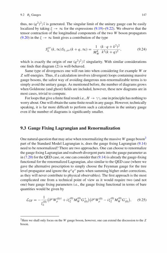
9.2 Rξ Gauges 147

thus, no (q2)2/ε is generated. The singular limit of the unitary gauge can be easilylocalized by taking ξ → ∞ for the expressions (9.19)–(9.22). We observe that thetensor contraction of the longitudinal components of the two W boson propagators(9.20) in the ξ → ∞ limit gives a contribution of the type

SμνL (k,∞)SL ,μν(k + q,∞) = 1

M4W

(k · q + k2)2

k2(k + q)2, (9.24)

which is exactly the origin of our (q2)2/ε singularity. With similar considerationsone finds that diagram (2) is well-behaved.

Same type of divergences one will run into when considering for example W orZ self-energies. Thus, if a calculation involves (divergent) loops containing massivegauge bosons, the safest way of avoiding dangerous non-renormalizable terms is tosimply avoid the unitary gauge. As mentioned before, the number of diagrams growswhen Goldstone (and ghost) fields are included, however, these new diagrams are inmost cases, trivial to compute.

For loops that give a finite final result i.e., H → γγ, one in principle has nothing toworry about. Onewill obtain the same finite result in any gauge. However, technicallyspeaking, it is far more difficult to perform such a calculation in the unitary gaugeeven if the number of diagrams is significantly smaller.

9.3 Gauge Fixing Lagrangian and Renormalization

One natural question thatmay arisewhen renormalizing themassive W gauge boson2

part of the Standard Model Lagrangian is, does the gauge fixing Lagrangian (9.14)need to be renormalized? There are two approaches. One can choose to renormalizethe gauge fixing Lagrangian and reabsorb divergent parts into the gauge parameter asin (7.20) for the QED case, or, one can consider that (9.14) is already the gauge-fixingfunctional for the renormalized Lagrangian, also similar to the QED case (where wegave the alternative prescription to simply choose the Feynman gauge for the treelevel propagator and ignore the qμqν parts when summing higher order corrections,as they will never contribute to physical observables). The first approach is the mostcomplicated one from a technical point of view as it would require two (and notone) bare gauge fixing parameters i.e., the gauge fixing functional in terms of barequantities would be given by

LGF = − 1

ξ(0)1

(∂μW (0)†

μ + iξ(0)2 M (0)

W G+(0)

)(∂μW (0)

μ − iξ(0)2 M (0)

W G−(0)

), (9.25)

2Here we shall only focus on the W gauge boson, however, one can extend the discussion to the Zboson.

148 9 Massive Spin One and Renormalizable Gauges

and only after renormalizing, one can choose the renormalized gauge fixing parame-ters to be equal (ξ1 = ξ2 = ξ). Thus, the renormalization procedure is in this casehighly complex. Here we shall present the alternative procedure.

We shall choose the Feynman gauge (ξ = 1) for this discussion.3 Expanding thegauge fixing functional from (9.14) we obtain

LGF = −∂μW †μ∂νWν − M2

W G+G− + i MW ∂μW †μG− − i MW ∂μWμG+. (9.26)

The gauge-Goldstonemixture from the StandardModel Lagrangian (that comes fromthe covariant derivatives) in terms of the bare quantities reads

L = −i M (0)W ∂μW (0)†

μ G−(0) + i M (0)

W ∂μW (0)μ G+

(0). (9.27)

Introducing the renormalization constants as

M (0)W = Z1/2

M MW , W (0)μ = Z1/2

W Wμ,

G±(0) = Z1/2

G± G±, (9.28)

(where Zi = 1 + δi ) the previous Lagrangian (9.27) in terms of the renormalizedparameters reads

L = −i Z1/2W Z1/2

M Z1/2G± MW ∂μW †

μG− + h.c.

= −i

(1 + 1

2δW + 1

2δM + 1

2δG±

)MW ∂μW †

μG− + h.c.

= −i MW ∂μW †μG− − i

2

(δW + δM + δG±

)MW ∂μW †

μG− + h.c.

= L + δL. (9.29)

The tree-level gauge-Goldstone mixing given by L is cancelled by the same mixingfrom the gauge fixing Lagrangian (9.26) and δL given by

δL = − i

2

(δW + δM + δG±

)MW ∂μW †

μG− + h.c.

≡ −i ZW G MW ∂μW †μG− + h.c. (9.30)

is a counterterm for the gauge-Goldstone mixing that appears at one-loop level. TheFeynman rule for this counterterm reads4

3Any other finite choice for the value of ξ is perfectly valid, however this is the choice that mostlysimplifies the gauge boson propagator.4An useful trick for deriving the Feynman rules corresponding to interaction terms that containderivatives of fields is given in Appendix C.

9.3 Gauge Fixing Lagrangian and Renormalization 149

W± G±

G± W±

p

p

∓ i pµ MW ZWG

Thus, the following sum is finite

W± G±

+ = finiteG±W±

+ = finiteG± W± W±G±

where the grey blobs from the LHS represent the sum of all the one-loop self-energydiagrams.

In the following we shall formally perform the Dyson resummation and renor-malize the W boson propagator, as this is a special case and the procedure is not asstraightforward as in the previously studied cases. The W boson self-energy can bewritten as

i�μνW ≡ igμν�T

W + ipμ pν

p2�L

W

≡ i

(gμν − pμ pν

p2

)�T

W + ipμ pν

p2�L

W (9.31)

with �LW = �L

W + �TW . Performing the Dyson resummation for the propagator in

the Feynman gauge we have

i Sμν = −igμν

p2 − M (0)2W

+ −igμλ

p2 − M (0)2W

(i�λρ

) −igρν

p2 − M (0)2W

+ −igμλ

p2 − M (0)2W

(i�λρ

) −igρσ

p2 − M (0)2W

(i�σδ

) −igδν

p2 − M (0)2W

+ . . .

= −igμν

p2 − M (0)2W

+ −i(

p2 − M (0)2W

)2(gμλ�λρg

ρν)

+ −i(

p2 − M (0)2W

)3(gμλ�λρg

ρσ�σδgδν

)+ . . .

150 9 Massive Spin One and Renormalizable Gauges

= −igμν

p2 − M (0)2W

⎛

⎜⎝1 + �TW

p2 − M (0)2W

+ (�TW )2

(p2 − M (0)2

W

)2 + . . .

⎞

⎟⎠

+ −i pμ pν

p2�L

W(p2 − M (0)2

W

)2

(1 + �L

W + 2�TW

p2 − M (0)2W

+ . . .

). (9.32)

Thus, we find

i Sμν = −igμν

p2 − M (0)2W − �T

W

+ −i pμ pν

p2×

× �LW(

p2 − M (0)2W − �T

W

)(p2 − M (0)2

W − �TW − �L

W

) (9.33)

The renormalized propagator is then given by

i Sμν = ZW−igμν

p2 − M2W − �T

W,R

+ ZW−i pμ pν

p2×

× �LW,R(

p2 − M2W − �T

W,R

)(p2 − M2

W − �TW,R − �L

W,R

)

≡ i ZW SμνR (9.34)

Using the standard procedure, one can now relate the ZW and Z M renormalizationconstants with the self-energies at the one-loop level. We shall shortly see with anexplicit example that the divergences of�T

W and�LW are related andonly one constant

ZW is needed for the wave function renormalization. Thus, it is worth mentioningthat the mass and wave function counterterms are totally determined by�T

W and onecan use only the gμν part of the propagator to calculate ZW and Z M . Starting at thetwo-loop level things are a little more complicated, as the previous Dyson summationmust also include one-loop transitions of the type W − G±:

G±W± W±

However, two-loop renormalization is far beyond the goal of this book.What about tadpoles? The widely spread approach (and the most simple) is to

perform a redefinition of the Higgs field of the Standard Model that generates acounterterm that cancels the tadpole contributions to the self-energies, as we did forthe φ3 model in Chap.7.5 Thus, if adopting this scheme, one only has to deal with

5This corresponds to the βh scheme from S. Actis, A. Ferroglia,M. Passera, G. Passarino, Two-LoopRenormalization in the Standard Model. Part I: Prolegomena, Nucl. Phys. B 777 (2007) 1, http://arxiv.org/pdf/hep-ph/0612122.pdf.

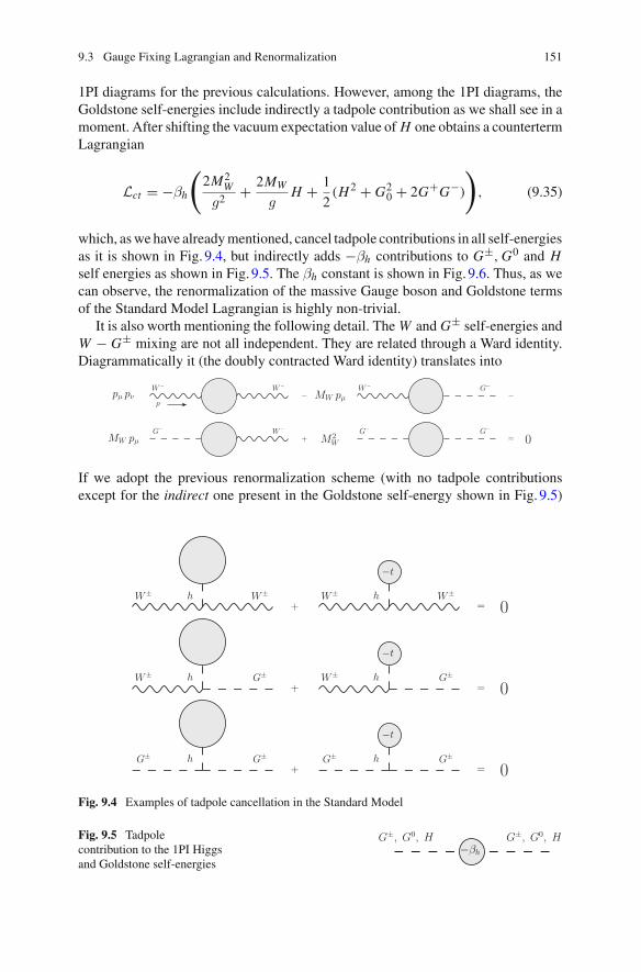
9.3 Gauge Fixing Lagrangian and Renormalization 151

1PI diagrams for the previous calculations. However, among the 1PI diagrams, theGoldstone self-energies include indirectly a tadpole contribution as we shall see in amoment. After shifting the vacuum expectation value of H one obtains a countertermLagrangian

Lct = −βh

(2M2

W

g2+ 2MW

gH + 1

2(H2 + G2

0 + 2G+G−)

), (9.35)

which, aswe have alreadymentioned, cancel tadpole contributions in all self-energiesas it is shown in Fig. 9.4, but indirectly adds −βh contributions to G±, G0 and Hself energies as shown in Fig. 9.5. The βh constant is shown in Fig. 9.6. Thus, as wecan observe, the renormalization of the massive Gauge boson and Goldstone termsof the Standard Model Lagrangian is highly non-trivial.

It is also worth mentioning the following detail. The W and G± self-energies andW − G± mixing are not all independent. They are related through a Ward identity.Diagrammatically it (the doubly contracted Ward identity) translates into

−G−W−

+G− W−

W− W−−

G− G−= 0M 2

W

MW pμpμ pν

MW pμ

p

If we adopt the previous renormalization scheme (with no tadpole contributionsexcept for the indirect one present in the Goldstone self-energy shown in Fig. 9.5)

+ = 0W± W±h

+hW± G±

hW± W±

W± G±h= 0

−t

−t

h G±G±+

h

−t

G±G±= 0

Fig. 9.4 Examples of tadpole cancellation in the Standard Model

Fig. 9.5 Tadpolecontribution to the 1PI Higgsand Goldstone self-energies

−βh

G±, G0, HG±, G0, H

152 9 Massive Spin One and Renormalizable Gauges

Fig. 9.6 Higgs tadpolecontribution in the StandardModel and definition of βh

Hi t = i βh

2MW

g=

one does not have to consider tadpoles either in the previous self-energies (exceptfor the indirect ones)!

In order to give a little more sense to the previously presented abstract renor-malization procedure and the Ward identity we shall take a simple one-loop explicitexample. Consider the following one-loop lepton-neutrino contribution to the W andG± self-energies, W − G± mixing and tadpole6

W−i Πμν

W

= i ΠG

W−=

i ΠμWG

H= i βh

2MW

g

= =W− W−G− G−

+G− G− G− G−

−βh

i t =

For the W self-energy one obtains the following expression

i�μνW = igμν�T

W + ipμ pν

p2�L

W , (9.36)

with the form functions �TW and �L

W given by

�TW = − g2

(4π)2μ2ε 1

ε

(1

2m2

l − 1

3p2

)+ finite, (9.37)

�LW = − g2

(4π)2μ2ε 1

ε

(1

3p2

)+ finite, (9.38)

where a2 = −p2x(1−x)+m2l x withml the mass of the lepton. The tadpole diagram

gives

t = 4m4l

(4π)2vμ2ε 1

ε+ finite. (9.39)

6The needed Feynman rules are given at the end of the chapter.

9.3 Gauge Fixing Lagrangian and Renormalization 153

with βh = gt/2MW . Summing the two corresponding diagrams for the Goldstoneself-energy we get

�G = g2

(4π)2

m2l

M2W

μ2ε 1

ε

(m2

l − 1

2p2

)− βh + finite

= − g2

(4π)2

m2l

M2W

μ2ε 1

ε

(1

2p2

)+ finite, (9.40)

where we have used g/2 = MW /v. The W − G± mixed term gives

�μW G = −pμ g2

(4π)2

m2l

MWμ2ε 1

ε

1

2+ finite. (9.41)

One can, thus, easily check that the following Ward identity holds

pμ pν�μνW + M2

W �G − 2MW pμ�μW G = 0 . (9.42)

Here we have checked this identity only for the UV-pole containing parts of theself-energies. It is left as an exercise for the reader to try to check this relation alsofor the finite parts. Let’s also explicitly check that

i�μW G + i MW pμZW G = finite . (9.43)

Separating the W and G± self energies as:

�TW = (p2 − M2

W )�TW,1 + �T

W,2, (9.44)

�G = (p2 − M2W )�G,1 + �G,2, (9.45)

we obtain the following counter-terms in the M S scheme

δW = �TW,1 = 1

3

g2

(4π)2μ2ε 1

ε, (9.46)

δM = −�TW,2

M2W

= − g2

(4π)2μ2ε 1

ε

(1

3− 1

2

m2l

M2W

), (9.47)

δG± = −�G,1 = g2

(4π)2μ2ε 1

ε

(1

2

m2l

M2W

), (9.48)

where we have used the expressions from (9.28) for the Zi constants and Zi = 1+δi .

154 9 Massive Spin One and Renormalizable Gauges

Thus

ZW G ≡ 1

2

(δM + δW + δG±

) = g2

(4π)2μ2ε 1

ε

(1

2

m2l

M2W

), (9.49)

and (9.43) follows immediately. As we mentioned earlier, one must note that δW alsocancels the infinities from �L

W (at one-loop level, when renormalizing the kineticand the mass terms of the W boson one obtains a counterterm with the Feynman rulegiven by i(pμ pν − gμν p2) + igμν M2

W (δW + δM ) that cancels the poles of i�μνW ).

Finally one should notice that the mass counter-term obtained from the Goldstoneboson propagator does not coincide with the one obtained from the W boson propa-gator. This is because the mass of the Goldstone is equal to the mass of the W boson,except, obviously, for quantum corrections which are different in the two cases. Thisshould be evenmore obvious in theml → 0 limit, for which the Goldstone couplingsto fermions vanish (thus �G = 0), and as it can be observed in (9.47) one of theterms in δM still survives.

The needed Feynman rules for the fermionic loop calculations are shown below

G−

l

ν

G−

−ig

2√

2ml

MW(1 − γ5)

−ig

2√

2ml

MW(1 + γ5)

l

ν

−ig

2√

2γμ(1 + γ5)

l, ν

ν, l

W

l

l

H −iml

v

Further Reading 155

Further Reading

K. Fujikawa, B.W.Lee,A.I. Sanda,Generalized renormalizable gauge formulation of spontaneouslybroken gauge theories. Phys. Rev. D 6, 2923 (1972)

J.M.Cornwall, J. Papavassiliou,D.Binosi,The Pinch Technique and its Applications to Non-AbelianGauge Theories. Cambridge Monographs on Particle Physics, Nuclear Physics and Cosmology

S. Actis, A. Ferroglia, M. Passera, G. Passarino, Two-loop renormalization in the standard model.part I: prolegomena. Nucl. Phys. B 777, 1 (2007), http://arxiv.org/pdf/hep-ph/0612122.pdf

D. Bardin, G. Passarino, The Standard Model in the Making, Precision Study of the ElectroweakInteractions, (Oxford University)Press

R. Santos, A. Barroso, On the renormalization of two Higgs doublet models. Phys. Rev. D 56, 5366(1997), http://arxiv.org/pdf/hep-ph/9701257.pdf

J.C. Romao, J.P. Silva, A resource for signs and Feynman diagrams of the Standard Model. Int. J.Mod. Phys. A 27, 1230025 (2012), http://arxiv.org/pdf/1209.6213.pdf

V. Ilisie, S.M. Higgs Decay and Production Channels, http://ific.uv.es/lhcpheno/PhDthesis/master_vilisie.pdf

Chapter 10Symmetries and Effective Vertices

Abstract When facing the computation of more realistic processes, the calculationscan become lengthy very fast as the number of Feynman diagrams grows. Beforestarting the calculation process the problem should be reduced to its minimal form.Here we will present an example of how to reduce the number of calculated diagramsfor a given process (which in this casewill be aHiggs-like scalar decay to two photonsthrough a charged scalar loop) using gauge symmetry.

10.1 Higgs Decay to a Pair of Photons

Consider the following interaction Lagrangian for scalar QED,with H± denoting thecharged scalar, plus an hypothetical interaction between a Higgs-like neutral scalarφ and a pair of H±

L = i e Aμ H+ ←→∂μ H− + e2 Aμ Aμ H+ H− − v λφH+ H− φ H+ H− (10.1)

where we have introduced the operator

a←→∂μ b ≡ a ∂μ b − (∂μ a) b. (10.2)

This interaction Lagrangian is actually part of the Two-Higgs-Doublet Model(2HDM) extension of the Standard Model (SM) with v the electroweak symme-try breaking scale.1 This extension assumes the presence of two Higgs doublets(instead of one, as in the SM), and it is characterized by three physical neutral scalars(instead of one) and a charged Higgs (H±). In the previous interaction Lagrangian φis assumed to be one of the neutral scalars of the model. The most important feature

1For a nice review of the SM read A. Pich, The Standard Model of Electroweak Interactions, http://arxiv.org/pdf/1201.0537.pdf. Also, for a nice review of the 2HDM read G.C. Branco, P.M. Ferreira,L. Lavoura, M.N. Rebelo, M. Sher and J.P. Silva, Theory and phenomenology of two-Higgs-doubletmodels, Phys. Rept. 516 (2012) 1, http://arxiv.org/pdf/1106.0034v3.pdf.

© Springer International Publishing Switzerland 2016V. Ilisie, Concepts in Quantum Field Theory,UNITEXT for Physics, DOI 10.1007/978-3-319-22966-9_10

157

158 10 Symmetries and Effective Vertices

Fig. 10.1 One-loop φ → γγeffective vertex

i Γ μν ≡k′ + q

q

k′

μ

ν

γ

γ

φ

of the 2HDM Lagrangian that we wish to exploit in this chapter, is that it preservesgauge invariance (just like the SM).

Let’s imagine that, given the previous interaction Lagrangian, wewish to calculatethe decay of the scalar φ to a pair of photons φ → γγ. This decay starts at theone loop level, as there are no tree-level interaction terms to account for it. Thus,we can conclude that the result is finite and needs no renormalization (the 2HDMis renormalizable). Before starting our calculation we can further exploit, as wementioned, gauge invariance, in order to simplify our computation. We can writedown an effective vertex describing the Lorentz structure of the final result. Considerthe following kinematic distribution for our process

φ(k′ + q) → γ(q,μ) γ(k′, ν) (10.3)

(with q2 = k′2 = 0 and (k′ + q)2 = M2φ and with μ, ν Lorentz indices) as shown in

Fig. 10.1. The most generic Lorentz structure that this effective vertex can contain is

Γ μν = S gμν k′ · q + A qμqν + B k′μk′ν + C qμk′ν

+ D qνk′μ + E εμναβk′αqβ, (10.4)

where S, A, B, . . . , E are Lorentz scalars. The last structure (∼εμναβ) would implythe presence of couplings proportional to γ5 matrices, thus we can safely discard it.Due to gauge invariance our effective vertex must satisfy

qμ Γ μν = qν Γ μν = 0. (10.5)

Also, all structures proportional to k′ν and qμ vanish when contacted with the polar-ization vectors of the photons (when calculating the transition matrix). Thus, oneobtains the following compact form for the effective vertex

i Γ μν = i (gμν k′ · q − qνk′μ) S . (10.6)

The transition matrix and its hermitian conjugate are thus given by

−i M = i (gμνk′ · q − k′μqν) S εr∗μ (q) εs∗

ν (k′)i M† = −i (gαβk′ · q − k′αqβ) S∗ εr

α(q) εsβ(k′). (10.7)

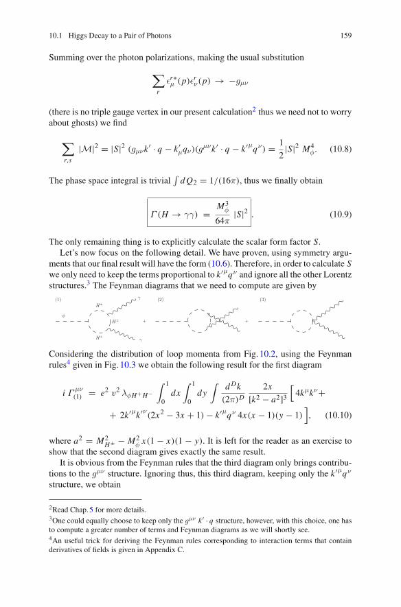
10.1 Higgs Decay to a Pair of Photons 159

Summing over the photon polarizations, making the usual substitution

∑

r

εr∗μ (p)εr

ν(p) → −gμν

(there is no triple gauge vertex in our present calculation2 thus we need not to worryabout ghosts) we find

∑

r,s

|M|2 = |S|2 (gμνk′ · q − k′μqν)(g

μνk′ · q − k′μqν) = 1

2|S|2 M4

φ. (10.8)

The phase space integral is trivial∫

d Q2 = 1/(16π), thus we finally obtain

Γ (H → γγ) = M3φ

64π|S|2 . (10.9)

The only remaining thing is to explicitly calculate the scalar form factor S.Let’s now focus on the following detail. We have proven, using symmetry argu-

ments that our final result will have the form (10.6). Therefore, in order to calculate Swe only need to keep the terms proportional to k′μqν and ignore all the other Lorentzstructures.3 The Feynman diagrams that we need to compute are given by

+H±

H±

H±

+φ

γ

γ

(1) (2) (3)

Considering the distribution of loop momenta from Fig. 10.2, using the Feynmanrules4 given in Fig. 10.3 we obtain the following result for the first diagram

i Γμν(1) = e2 v2 λφH+ H−

∫ 1

0dx

∫ 1

0dy

∫d Dk

(2π)D

2x

[k2 − a2]3[4kμkν+

+ 2k′μk′ν(2x2 − 3x + 1) − k′μqν 4x(x − 1)(y − 1)], (10.10)

where a2 = M2H± − M2

φ x(1 − x)(1 − y). It is left for the reader as an exercise toshow that the second diagram gives exactly the same result.

It is obvious from the Feynman rules that the third diagram only brings contribu-tions to the gμν structure. Ignoring thus, this third diagram, keeping only the k′μqν

structure, we obtain

2Read Chap.5 for more details.3One could equally choose to keep only the gμν k′ · q structure, however, with this choice, one hasto compute a greater number of terms and Feynman diagrams as we will shortly see.4An useful trick for deriving the Feynman rules corresponding to interaction terms that containderivatives of fields is given in Appendix C.

160 10 Symmetries and Effective Vertices

Fig. 10.2 Contribution ofthe first diagram to theφ → γγ process

k + q

k

k − k′

k′ + q

φ

k′ν γ∗

qμ γ

H+

H+

H+

i Γμν(1)=

Fig. 10.3 Feynman rules forthe interaction Lagrangian

μ

p

qH+

H+

γ −i e (p + q)μ ,

H±

H±

φ −i v λφH+H− ,

ν

H±

H± γ

μ

γ

i e2 gμν .

i Γμν(1+2) = −e2v2 λφH+ H−

∫ 1

0dx

∫ 1

0dy

∫d Dk

(2π)D

16x2(x − 1)(y − 1)

[k2 − a2]3 k′μqν

= i e2v2 λφH+ H−∫ 1

0dx

∫ 1

0dy

16x2(x − 1)(y − 1)

32 π2 a2 k′μqν (10.11)

Thus, the scalar form factor S is simply given by

S = − e2 v2 λφH+ H−∫ 1

0dx

∫ 1

0dy

x2(x − 1)(y − 1)

2 π2 a2 . (10.12)

Again, the reader is invited to explicitly check that this is exactly the result oneobtains by doing the full calculation.

In this example, using the symmetries of our Lagrangian, we were able to getrid of one Feynman diagram and all the other Lorentz structures except k′μqν .

10.1 Higgs Decay to a Pair of Photons 161

The UV-divergent parts of the structure kμkν obviously cancels against the UV-divergent parts of the third diagram (that we have ignored).

It might seem at first sight that we haven’t gained that much. This was, howevera very simple example. If one has to calculate the full SM contribution to this decay(which involves fermions and W bosons) this technique tremendously simplifies thecalculations. Other interesting examples can be found in the first two references.

Further Reading

V. Ilisie, A. Pich, Low-mass fermiophobic charged Higgs phenomenology in two-Higgs-doubletmodels. JHEP 1409, 089 (2014). http://arxiv.org/pdf/1405.6639v3.pdf

V. Ilisie, New Barr-Zee contributions to (g − 2)μ in two-Higgs-doublet models. JHEP 04, 077(2015) http://arxiv.org/pdf/1502.04199v3.pdf

A. Pich, The Standard Model of Electroweak Interactions, http://arxiv.org/pdf/1201.0537.pdfG.C. Branco, P.M. Ferreira, L. Lavoura, M.N. Rebelo, M. Sher, J.P. Silva, The-

ory and phenomenology of two-Higgs-doublet models. Phys. Rep. 516, 1 (2012)http://arxiv.org/pdf/1106.0034v3.pdf

C. Itzykson, J. Zuber, Quantum Field TheoryM.E. Peskin and D.V. Schroeder, An Introduction to Quantum Field Theory

Chapter 11Effective Field Theory

Abstract Effective field theories (EFTs) are a highly important topic in QuantumField Theory. Here we are going to shortly present some important highlights as wellas the renormalization group equations for the Wilson coefficients. Afterwards weshall focus on one illustrative example and present the matching procedure at theone-loop level. The infrared behaviour of EFTs is also covered with this example.

11.1 Effective Lagrangian

For a nice introduction as well as more advanced topics consult references. Aneffective field theory is characterized by some effective Lagrangian:

Leff =∑

i

ci

Λdi −4Oi ≡∑

i

CiOi , (11.1)

where Oi are operators constructed with the light fields, and the information onthe heavy degrees of freedom is hidden in the couplings Ci ; di is the dimension ofthe operator Oi and Λ is the scale where the heavy fields come into the game. Forsimplicitywe have considered that there is only one operator for a given dimension. Ifthis was not the case, another summation (over all the operators of a given dimension)should be included in the Lagrangian i.e.,

Leff =∑

i, j

c( j)i

Λdi −4O( j)i ≡

∑

i, j

C( j)i O( j)

i . (11.2)

The operators are classified depending on their dimension as:

di < 4 → relevant, di = 4 → marginal, di > 4 → irrelevant. (11.3)

The Lagrangian Leff contains an infinite number of terms (power series in Λ), there-fore it is not renormalizable in the usual sense (an infinite number of counterterms

© Springer International Publishing Switzerland 2016V. Ilisie, Concepts in Quantum Field Theory,UNITEXT for Physics, DOI 10.1007/978-3-319-22966-9_11

163

164 11 Effective Field Theory

would also be needed for renormalization). If we truncate the series of the Lagrangiani.e., we only include terms up to dimension N

Leff =N∑

i

CiOi , (11.4)

with N finite, the Lagrangian is not, in general, renormalizable either. However, fora given loop order the needed number of renormalization counterterms is finite.1

In effective theories the number of counterterms needed for renormalization growswith the number of loop corrections included, whereas, for renormalizable theories(in the usual sense) the number of conterterms is the same at any loop order.

11.2 Renormalization Group Equations

11.2.1 No Operator Mixing

In the following we shall consider the renormalization group equations (RGEs) forthe coefficients Ci and the operatorsOi . For this first analysis we shall only considera simple case for which the coefficients do not mix under renormalization. Normallythis is case when there is only one operator for a given dimension di and is whatwe are going to consider next. Given the bare operator OB

i and the bare Wilsoncoefficient CB

i , when including loop corrections the Lagrangian can be written interms of the renormalized quantities as:

Leff =∑

i

CBi OB

i =∑

i

CBi Zi (μ)Oi (μ) =

∑

i

Ci (μ)Oi (μ) , (11.5)

where we have defined the Zi renormalization constant as

OBi = Zi (μ)Oi (μ), (11.6)

and where the renormalized Wilson coefficient is given by

CBi = Zi (μ)−1Ci (μ). (11.7)

This is the standard approach when renormalizing effective Lagrangians; oneincludes the loop corrections, and hence the μ-dependence, that comes from the

1This is true provided that we use mass-independent renormalization schemes i.e., the MS scheme.In order to understand why mass-independent schemes are needed for renormalization of EFTsconsult for example section 3. Quantum Loops of Effective Field Theory (A. Pich, http://arxiv.org/abs/hep-ph/9806303).

11.2 Renormalization Group Equations 165

operator renormalization into the Wilson coefficient so that the renormalizedLagrangian is μ-independent. All the loop corrections are then contained in the Ci

coefficients (as we shall shortly see with an example). Let us write down the formalRGEs2 for Ci and Oi . The bare operator is μ-independent, therefore:

μdOB

i

dμ= 0 = μOi

d Zi

dμ+ μZi

dOi

dμ. (11.8)

We define the gamma function of the operator Oi as

γOi = μ

Zi

d Zi

dμ= γ

(1)Oi

(α

π

)+ γ

(2)Oi

(α

π

)2 + . . . , (11.9)

where α is the expansion parameter of the operator. Thus, the RGE for the operatorOi is simply given by:

μdOi

dμ= −γOiOi . (11.10)

On the other hand, the productOBi CB

i = Oi (μ)C(μ) isμ-independent, thuswe obtainanalogous RGEs for the Wilson coefficients Ci :

μdCi

dμ= γOi Ci . (11.11)

The solution of this equation is given in (B.23):

Ci (μ) = Ci (μ0) exp

{∫ α(μ)

α(μ0)

dα

α

γOi (α)

β(α)

}

= Ci (μ0)[ α(μ)

α(μ0)

]γ(1)Oi

/β1{1 + . . .

}(11.12)

11.2.2 Operator Mixing

Let’s now consider that there are n operators for a given dimension di . Introducingthe short-hand notation O( j)

i ≡ O j (with j = 1, . . . , n), the effective Lagrangianfor the given dimension di can be written as

2For a short reminder of RGEs see Appendix B.

166 11 Effective Field Theory

Li,eff =∑

j

C( j)i O( j)

i ≡∑

j

C jO j ≡ CTO, (11.13)

where we have definedO as a 1-column vector and CT as a 1-row vector. In generalthe operators mix under renormalization, i.e.,

OBi =

n∑

j

Zij(μ)O j (μ) ⇒ CBi =

n∑

j

(Z−1)

ji(μ)C j (μ). (11.14)

In this case it turns out to be very useful to use the matrix notation:

OB = Z(μ)O(μ) ⇒ CB = (Z−1)T

(μ)C(μ). (11.15)

We easily obtain the RGEs for the operators and the Wilson coefficients

(μ

d

dμ+ γO

)O(μ) = 0 ,

(μ

d

dμ− γT

O)C(μ) = 0

(11.16)

where the anomalous dimension matrix γO is given by:

γO ≡ Z−1μd

dμZ. (11.17)

In order to solve this equation we must find the matrix U that diagonalizes γO i.e.,

U−1γTOU = γO, (11.18)

with γO diagonal. Introducing the previous equation into (11.16) we find:

(UU−1μ

d

dμ− UγOU−1

)C(μ) = 0. (11.19)

Defining C = U−1C we find the following equations in diagonal form:

(μ

d

dμ− γO

)C(μ) = 0 (11.20)

Thus, the coefficients Ci obey the unmixed RGEs:

(μ

d

dμ− γ

(i)O

)Ci (μ) = 0, (11.21)

11.2 Renormalization Group Equations 167

where γ(i)O are the diagonal terms of the matrix γO. The solution is straightforward

(same as in the previous section):

Ci (μ) = Ci (μ0) exp

{∫ α(μ)

α(μ0)

dα

α

γ(i)O (α)

β(α)

}. (11.22)

Changing the basis from Ci to Ci we finally find the solution we were looking for:

Ci (μ) =∑

j,k

Uij exp

{∫ α(μ)

α(μ0)

dα

α

γ( j)O (α)

β(α)

}(U−1)

jkCk(μ0) . (11.23)

11.3 Matching

11.3.1 ϕφ2 Theory

Consider the following Lagrangian:

L = 1

2(∂φ)2 − 1

2m2φ2 + 1

2(∂ϕ)2 − 1

2M2ϕ2 − 1

2λϕφ2 (11.24)

If M � m, E , where E is the energy domain of the process we want to analyse,we can integrate out (from the path integral) the heavy field ϕ and write down aneffective Lagrangian that describes physical processes at energies E ∼ m. Say wewish to describe a scattering process like φ(p1)φ(p2) → φ(p3)φ(p4), then we canwrite the following effective Lagrangian:

Leff = 1

2C0(∂φ)2 − 1

2C2φ2 − 1

4!C0φ4 + . . . , (11.25)

where C0, C0 are the Wilson coefficients of zero dimension and C2 is the two-dimensional one. These coefficients can be expanded as:

C0 = C(0)0 + C(1)

0 + . . . , C0 = C(0)0 + C(1)

0 + . . . , C2 = C(0)2 + C(1)

2 + . . . ,

(11.26)

where the upper index stands for the corresponding loop order. In the following weshall present the matching procedure. Both theories must give identical results at amatching scaleμ ∼ M . Thus at this given scale the scattering amplitudes provided byL andLeff must be the same. At tree-level however, thematching is scale independent(the scale dependence comes into the game only at the loop level). The tree-levelmatching is diagrammatically shown in Fig. 11.1. Explicitly this reads:

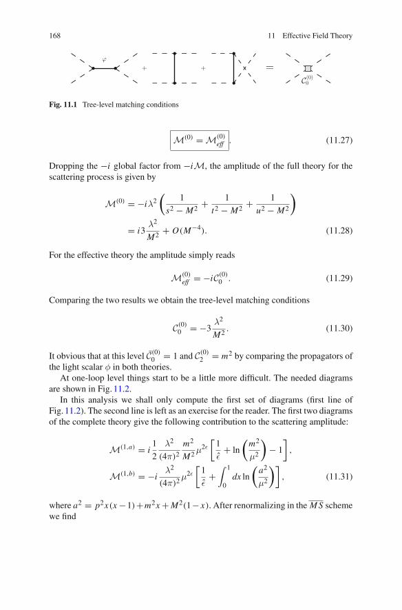
168 11 Effective Field Theory

+ =C(0)0

+ϕ

Fig. 11.1 Tree-level matching conditions

M(0) = M(0)eff . (11.27)

Dropping the −i global factor from −iM, the amplitude of the full theory for thescattering process is given by

M(0) = −iλ2(

1

s2 − M2 + 1

t2 − M2 + 1

u2 − M2

)

= i3λ2

M2 + O(M−4). (11.28)

For the effective theory the amplitude simply reads

M(0)eff = −iC(0)

0 . (11.29)

Comparing the two results we obtain the tree-level matching conditions

C(0)0 = −3

λ2

M2 . (11.30)

It obvious that at this level C(0)0 = 1 and C(0)

2 = m2 by comparing the propagators ofthe light scalar φ in both theories.

At one-loop level things start to be a little more difficult. The needed diagramsare shown in Fig. 11.2.

In this analysis we shall only compute the first set of diagrams (first line ofFig. 11.2). The second line is left as an exercise for the reader. The first two diagramsof the complete theory give the following contribution to the scattering amplitude:

M(1,a) = i1

2

λ2

(4π)2

m2

M2μ2ε[1

ε+ ln

(m2

μ2

)− 1

],

M(1,b) = −iλ2

(4π)2μ2ε

[1

ε+

∫ 1

0dx ln

(a2

μ2

)], (11.31)

where a2 = p2x(x −1)+m2x + M2(1− x). After renormalizing in the M S schemewe find

11.3 Matching 169

+ =C(0)0

+

C(1)2 , C(1)

0

(1, a) (1, b) (1, a)eff (2, a)eff

C(0)0

+ ........= ++........

C(0)0 C(1)

0

p

Fig. 11.2 One-loop matching conditions

M(1,a)R = i

1

2

λ2(μ)

(4π)2

m2(μ)

M2

[ln

(m2(μ)

μ2

)− 1

],

M(1,b)R = −i

λ2(μ)

(4π)2

∫ 1

0ln

(a2(μ)

μ2

), (11.32)

where λ(μ) and m(μ) are the running coupling and the running mass of the fulltheory (as usual, the subscript R stands for renormalized or regular).3 In order toperform the matching properly we must expand the logarithm of a2/μ2 in powers ofp2/M2:

∫ 1

0dx ln

(a2

μ2

)=

∫ 1

0dx ln

(p2x(x − 1) + m2x + M2(1 − x)

μ2

)

= ln

(M2

μ2

)+

∫ 1

0dx ln

(p2

M2 x(x − 1) + m2

M2 x + (1 − x)

)

≈ ln

(M2

μ2

)+

∫ 1

0dx ln

(m2

M2 x + (1 − x)

)

+∫ 1

0dx

(p2/M2)x(x − 1)

(m2/M2)x + 1 − x

= ln

(M2

μ2

)− m2

M2 ln

(m2

M2

)− 1 − 1

2

p2

M2 + O(M−4). (11.33)

3In general, after renormalization M will also depend on μ. However we have considered thatM(μ) ≈ constant close to the matching scale μ ∼ M .

170 11 Effective Field Theory

Summing both contributions, (1, a) and (1, b), one obtains:

M(1)R = M(1,a)

R + M(1,b)R

= iλ2(μ)

(4π)2

[3

2

m2(μ)

M2 ln

(m2(μ)

μ2

)− 1

2

m2(μ)

M2

+1 + 1

2

p2

M2 − ln

(M2

μ2

)](11.34)

We will now move on to the computation of the diagrams for the effective theory.The transition amplitude of the first diagram reads:

M(1,a)eff = 1

2C(0)0

∫d Dk

(2π)D

1

k2 − m2

= i3

2

λ2

(4π)2

m2

M2μ2ε[1

ε+ ln

(m2

μ2

)− 1

]. (11.35)

The second one is simply:

M(1,b)eff = −iC(1)2 + i p2C(1)

0 . (11.36)

After renormalizing in the MS scheme, we obtain

M(1)eff,R = M(1,a)eff

R + M(1,b)eff

= i3

2

λ2eff(μ)

(4π)2

m2eff(μ)

M2

[ln

(m2

eff(μ)

μ2

)− 1

]

− iC(1)2 (μ) + i p2C(1)

0 (μ) (11.37)

where λeff(μ) and meff(μ) are the running coupling and mass in the effective theory(which, in general are not equal to the ones in the full theory). For the matching,in order to avoid potentially large logarithmic contributions from ln(M2/μ2) wemust choose the matching scale μ around M . Here we shall choose it μ = M . Thematching condition M(1)

eff,R = M(1)R then gives:

3

2

λ2eff(M)

(4π)2

m2eff(M)

M2

[ln

(m2

eff(M)

M2

)− 1

]

− C(1)2 (M) + p2C(1)

0 (M)

= λ2(M)

(4π)2

[3

2

m2(M)

M2 ln

(m2(M)

M2

)

−1

2

m2(M)

M2 + 1 + 1

2

p2

M2

](11.38)

11.3 Matching 171

Therefore we get to the following relations between the parameters of the full andeffective theory

λ(M) = λeff(M), m(M) = meff(M), (11.39)

for the mass and coupling and

C(1)0 (M) = 1

2

λ2(M)

(4π)2M, (11.40)

C(1)2 (M) = −λ(M)

(4π)2

(1 + m2(M)

M2

), (11.41)

for the coefficients. Onemust notice that the terms proportional to ln(m2/M2) cancelexactly in the matching. This is a general feature of effective theories: both thecomplete theory and the effective one have the same IR behaviour (thus also thesame IR divergences) and therefore, the IR divergences will always cancel inthe matching. In this case, if we wanted to take the limit m → 0 for the light fieldφ, it would give rise to an IR divergent logarithm. However, this logarithm cancelsin the matching and our effective theory is IR safe (well defined in the limit m → 0).

Thus, after the matching we are left with the following effective Lagrangian

Leff =1

2

[1 + 1

2

λ2eff(μ)

(4π)2M2

](∂φ)2

− 1

2

[m2

eff(μ) − λ2eff(μ)

(4π)2

(1 + m2

eff(μ)

M2

)]φ2

− 1

4!

[−3

λ2eff(μ)

M2 + aλ4

eff(μ)

(4π)2M4

]φ4 + . . . , (11.42)

where a is determined by the matching given in the second line of Fig. 11.2 whichhas been left as an exercise. The running parameters λeff(μ) and meff(μ) can becalculated solving the RGEs with the initial conditions given by (11.39). The lowscale is usually chosen as μ2 ∼ m2. Note that the Lagrangian (11.42) doesn’t havea canonically normalized kinetic term. In order to obtain the canonical kinetic termand, therefore, use the standard Feynman rules we must perform a field redefinition:

φ → φ

√

1 − 1

2

λ2eff(μ)

(4π)2M2 . (11.43)

172 11 Effective Field Theory

Thus, our final Lagrangian takes the form

Leff = 1

2(∂φ)2 − 1

2

[m2

eff(μ) − λ2eff(μ)

(4π)2

(1 + m2

eff(μ)

M2

)

−1

2

λ2eff(μ)m2

eff(μ)

(4π)2M2

]φ2 − 1

4!

[−3

λ2eff(μ)

M2

+ (3 + a)λ4

eff(μ)

(4π)2M4

]φ4 + . . .

≡ 1

2(∂φ)2 − 1

2m2

eff(μ) φ2 − 1

4! λeff(μ) φ4 + . . . (11.44)

for which we can define the usual Feynman rules following the standard procedureand that we can use for calculating scattering processes like φφ → φφwith one-loopmatching precision.

Further Reading

A. Pich, Effective Field Theory, arxiv:hep-ph/9806303I. Stewart, Effective Field Theories Lecture Notes, http://pages.physics.cornell.edu/~ajd268/Notes/EffectiveFieldTheories.pdf

C. Scrucca, Advanced Quantum Field Theory, http://itp.epfl.ch/files/content/sites/itp/files/users/181759/public/aqft.pdf

A.J. Buras, Weak Hamiltonian, CP Violation and Rare Decays, arxiv:hep-ph/9806471W. Skiba, TASI Lectures on Effective Field Theory and Precision Electroweak Measurements,arxiv:org/pdf/1006.2142v1.pdf

Chapter 12Optical Theorem

Abstract The optical theorem can turn out to be a handy tool in calculating absorp-tive (imaginary) parts of self-energies (or scattering amplitudes) or it can be a usefulcross check for some calculations. In this chapter we will explicitly deduce the stan-dard form of the optical theorem and try to establish a robust and transparent notation.We will also take an illustrative example and recover the well known Breit-Wignerapproximation for unstable particle propagators.

12.1 Optical Theorem Deduction

The scattering matrix S can be written as S = I − iM, where I is the identityoperator and M the transition matrix. The unitarity property of S guarantees thatS†S = I, to all orders in perturbation theory. Therefore, we can write the following:

S†S = (I + iM†)(I − iM) = I − iM + iM† + M†M = I. (12.1)

Thus:

i(M − M†) = M†M. (12.2)

Given an initial state |i〉 and a final state | f 〉, we have

i〈 f |(M − M†)|i〉 = 〈 f |M†M|i〉. (12.3)

Introducing the closure relation in between M† and M on the RHS of (12.3) we get

i〈 f |(M − M†)|i〉 =∑

n

〈 f |M†|n〉〈n|M|i〉, (12.4)

© Springer International Publishing Switzerland 2016V. Ilisie, Concepts in Quantum Field Theory,UNITEXT for Physics, DOI 10.1007/978-3-319-22966-9_12

173

174 12 Optical Theorem

where |n〉 is a complete basis of orthogonal states, and where∑

n is defined as

∑

n

≡∑

n

1

(2π)3n j

∫ n j∏

l=1

d3 pl

2El. (12.5)

In the previous expression n j represents the number of particles in the state |n〉. Ifwe suppose that the initial and final states are the same, then the LHS of (12.4) reads:

i〈i |(M − M†)|i〉 = i[〈i |M|i〉 − 〈i |M†|i〉]

= i(2π)4δ(4)(Pi − Pi )[Mi→i − M†

i→i

]

= −2Im(Mi→i

)(2π)4δ(4)(Pi − Pi ) (12.6)

where we have introduced the following notation:

〈 f |M|i〉 = (2π)4 δ(4)(P f − Pi ) Mi→ f . (12.7)

On the other hand, looking at the RHS of (12.4) we obtain the following:

∑

n

〈i |M†|n〉〈n|M|i〉 =∑

n

〈n|M|i〉†〈n|M|i〉

=∑

n

((2π)4δ(4)(Pi − Pn)

)2|Mi→n|2. (12.8)

Thus, combining (12.8) and (12.6) we obtain the standard form of the Optical The-orem:

−2Im(Mi→i ) =∑

n

1

(2π)3n j −4

∫ n j∏

l=1

d3 pl

2Elδ(4)(Pi − Pn)|Mi→n|2. (12.9)

If the initial state is a two-particle state (a + b), the theorem takes the form1:

−2 Im(Mi→i ) = 2λ1/2(s, m2a, m2

b)∑

n

σ(a + b → n)

= 2λ1/2(s, m2a, m2

b)σ(a + b → all), (12.10)

What the previous expression states is that, except for the λ1/2(s, m2a, m2

b) factor anda global sign, the absorptive (imaginary) part of the transition matrix is equal (orderby order in perturbation theory) to the sum of the cross sections describing all thepossible final states originated by the initial two body scattering. Schematically:

1See Chap.3 for definitions of decay rates and cross sections.

12.1 Optical Theorem Deduction 175

Im ∼ ∑ ...

2

If the initial state is a one-particle state (a), then we can relate self-energies withdecay widths:

Im ∼ ∑

2

.

.

.

Therefore, the imaginary part of the self-energy is proportional to the total decaywidth of the particle:

−2Im(Mi→i ) = 2√

k2∑

n

Γ (a → n) = 2√

k2 Γ (a → all) ≡ 2√

k2 Γa(k2),

(12.11)

where k2 and Γa are the squared four-momentum and the total decay width of theparticle a. Note that in the previous equation we have written

√k2 instead of the

mass ma . This is because, on the LHS of the previous equation, we have the self-energy amplitude of a particle that is not necessarily on-shell (k2 �= m2

a in general).Thus, the total decay width must also be expressed as a function of

√k2 and not of

ma . This will be better understood with a latter example.Therefore, (12.11) justifies the Breit-Wigner approximation of the propagator of

an unstable particle. Consider for example the propagator of a scalar particle φ.After accounting for loop effects and renormalizing, the propagator contains therenormalized2 two point function Π R

φ (k2):

i

k2 − M2 + Π Rφ (k2)

= i

k2 − M2 + ReΠ Rφ (k2) + i Im Π R

φ (k2). (12.12)

As a first order approximation, we can ignore the real part of the two-point functionand we obtain the well-known expression:

i

k2 − M2φ + i

√k2Γφ(k2)

≈ i

k2 − M2φ + i MφΓφ

. (12.13)

2See Chap.7 for more details on renormalization.

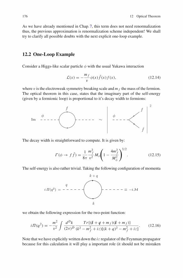
176 12 Optical Theorem

As we have already mentioned in Chap.7, this term does not need renormalizationthus, the previous approximation is renormalization scheme independent! We shalltry to clarify all possible doubts with the next explicit one-loop example.

12.2 One-Loop Example

Consider a Higgs-like scalar particle φ with the usual Yukawa interaction

L(x) = −m f

vφ(x) f (x) f (x), (12.14)

where v is the electroweak symmetry breaking scale and m f the mass of the fermion.The optical theorem in this case, states that the imaginary part of the self-energy(given by a fermionic loop) is proportional to it’s decay width to fermions:

Im ∼

2

φ

f f

f

φ

The decay width is straightforward to compute. It is given by:

Γ (φ → f f ) = 1

8π

m2f

v2Mφ

(1 − 4m2

f

M2φ

)3/2

. (12.15)

The self-energy is also rather trivial. Taking the following configuration of momenta

i Π(q2) =q

k + q

k

≡ −i M

we obtain the following expression for the two-point function:

iΠ(q2) = −m2

v2

∫d Dk

(2π)D

T r{(/k + /q + m f )(/k + m f )}(k2 − m2

f + iε)[(k + q)2 − m2f + iε] . (12.16)

Note that we have explicitly written down the iε regulator of the Feynman propagatorbecause for this calculation it will play a important role (it should not be mistaken

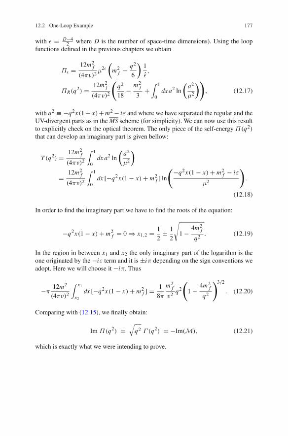
12.2 One-Loop Example 177

with ε = D−42 where D is the number of space-time dimensions). Using the loop

functions defined in the previous chapters we obtain

Πε = 12m2f

(4πv)2μ2ε

(m2

f − q2

6

)1

ε,

ΠR(q2) = 12m2f

(4πv)2

(q2

18− m2

f

3+

∫ 1

0dx a2 ln

(a2

μ2

)), (12.17)

with a2 ≡ −q2x(1− x) + m2 − iε and where we have separated the regular and theUV-divergent parts as in the MS scheme (for simplicity). We can now use this resultto explicitly check on the optical theorem. The only piece of the self-energy Π(q2)

that can develop an imaginary part is given bellow:

T (q2) = 12m2f

(4πv)2

∫ 1

0dx a2 ln

(a2

μ2

)

= 12m2f

(4πv)2

∫ 1

0dx [−q2x(1 − x) + m2

f ] ln(−q2x(1 − x) + m2

f − iε

μ2

).

(12.18)

In order to find the imaginary part we have to find the roots of the equation:

−q2x(1 − x) + m2f = 0 ⇒ x1,2 = 1

2± 1

2

√

1 − 4m2f

q2 . (12.19)

In the region in between x1 and x2 the only imaginary part of the logarithm is theone originated by the −iε term and it is ±iπ depending on the sign conventions weadopt. Here we will choose it −iπ. Thus

−π12m2

(4πv)2

∫ x1

x2dx [−q2x(1 − x) + m2

f ] = 1

8π

m2f

v2q2

(1 − 4m2

f

q2

)3/2

. (12.20)

Comparing with (12.15), we finally obtain:

Im Π(q2) =√

q2 Γ (q2) = −Im(M), (12.21)

which is exactly what we were intending to prove.

178 12 Optical Theorem

Further Reading

C. Itzykson, J. Zuber, Quantum Field TheoryM.E. Peskin, D.V. Schroeder, An Introduction to Quantum Field TheoryV. Ilisie, S.M. Higgs Decay and Production Channels, http://ific.uv.es/lhcpheno/PhDthesis/master_vilisie.pdf

L.H. Ryder, Quantum Field Theory (Cambridge University Press, Cambridge, 1985)T.P. Cheng, L.F. Li,Gauge Theory of Elementary Particle Physics (OxfordUniversity Press, Oxford,1984)

F. Mandl, G.P. Shaw, Quantum Field Theory

Appendix AMaster Integral

Consider the integral J (D,α,β, a2) defined in (6.1):

J (D,α,β, a2) ≡∫

d Dk

(2π)D

(k2)α

(k2 − a2)β. (A.1)

Given a four-vector kμ we introduce the following Euclidean quantities (this is oftencalled a Wick rotation):

kμ = (k0, k) = (ik0E , kE ). (A.2)

Therefore, we find the following:

k2 = (k0)2 − k2 = −(k0E )2 − k2E ≡ −k2E , (A.3)

dk0 = idk0E , (A.4)

d Dk = id DkE . (A.5)

We can thus, write (A.1) in terms of the previously introduced parameters

J (D,α,β, a2) = i∫

d DkE

(2π)D

(−1)α(k2E )α

(−k2E − a2)β

= (−1)α−βi∫

d DkE

(2π)D

(k2E )α

(k2E + a2)β. (A.6)

Let’s now consider the following integral in spherical coordinates:

∫ +∞

−∞d Dx =

∫dΩD

∫ ∞

0d|x ||x |D−1 ≡ SD

∫ ∞

0d|x ||x |D−1, (A.7)

© Springer International Publishing Switzerland 2016V. Ilisie, Concepts in Quantum Field Theory,UNITEXT for Physics, DOI 10.1007/978-3-319-22966-9

179

180 Appendix A: Master Integral

where we have defined SD ≡ ∫dΩD and where ΩD is a solid angle. Using

√π =

∫ +∞

−∞dxe−x2 ,

∫ ∞

0dxx D−1e−x2 = 1

2Γ (D/2), (A.8)

we obtain that (√

π)D can be written as

(√

π)D =(∫ +∞

−∞dxe−x2

)D

≡∫ +∞

−∞d Dxe−x2

=∫

dΩD

∫ ∞

0dxx D−1e−x2

= SD

2Γ (D/2). (A.9)

Thus SD is simply given by SD = 2πD/2/Γ (D/2). Introducing the previous resultwe can now write (A.6) as:

J (D,α,β, a2) = 2i(−1)α−βπD/2

(2π)DΓ (D/2)

∫ ∞

0d|kE ||kE |D−1 |kE |2α

(|k2E | + a2)β

= 2i(−1)α−β

(4π)D/2Γ (D/2)

∫ ∞

0d|kE | |kE |2α+D−1

(|k2E | + a2)β. (A.10)

All we have left to do is to find the solution to the remaining integral

K ≡∫ ∞

0d|kE | |kE |2α+D−1

(|k2E | + a2)β. (A.11)

Performing a change of variable

z ≡ a2

(|kE |2 + a2), (A.12)

we find:

lim|kE |→∞ z = 0, lim|kE |→0z = 1, dz = − 2a2|kE |

(|kE |2 + a2)2d|kE |. (A.13)

Appendix A: Master Integral 181

Thus, we can write |kE | and d|kE | as

|kE | =(

a2

z(1 − z)

)1/2

, d|kE | = −1

2dz(1 − z)−1/2(a−2)

(a2

z

)3/2

.

(A.14)

The integral K in terms of the new variable takes the form

K = −∫ 0

1

1

2dz(a2)α−β+D/2zβ−α−D/2−1(1 − z)α+D/2−1

=∫ 1

0

1

2dz(a2)α−β+D/2zβ−α−D/2−1(1 − z)α+D/2−1. (A.15)

Therefore the expression (A.10) becomes

J (D,α,β, a2) = i(−1)α−β(a2)α−β+D/2

(4π)D/2Γ (D/2)

∫ 1

0dzzβ−α−D/2−1(1 − z)α+D/2−1.

(A.16)

Introducing the Euler Beta function,

B(m, n) =∫ 1

0dzzm−1(1 − z)n−1 = Γ (m)Γ (n)

Γ (n + m), (A.17)

taking m = β − α − D/2, n = α + D/2 we finally obtain the expression that wewere looking for:

J (D,α,β, a2) = i

(4π)D/2 (a2)D/2(−a2)α−β Γ (β − α − D/2)Γ (α + D/2)

Γ (β)Γ (D/2).

(A.18)

Appendix BRenormalization Group Equations

In the following we present a compendium of useful formulae regarding the renor-malization group equations (RGEs) for the coupling constant, mass and a genericGreen function.

B.1 Beta Function

Consider a model with one expansion parameter α, i.e., the QED Lagrangian intro-duced in Chap.7. After including quantum corrections we need to perform renor-malization. If α0 is the bare parameter and α is the renormalized one, we have learntthat both parameters are related through a renormalization constant, say Zα that weshall define as

α0 = Zαα, (B.1)

(in the QED case for example, we have Zα = Z−13 ). As the renormalization con-

stants are renormalization scale dependent (proportional to a μ2ε factor) and the bareparameter is μ-independent, we conclude that the renormalized parameter must alsodepend on μ so that the product Zαα is scale independent:

α0 = Zα(μ)α(μ) . (B.2)

In order to find the scale dependence of the renormalized coupling we differentiatewith respect to μ on both sides of the previous equation:

μdα0

dμ= 0 = μZα

dα

dμ+ μα

d Zα

dμ. (B.3)

© Springer International Publishing Switzerland 2016V. Ilisie, Concepts in Quantum Field Theory,UNITEXT for Physics, DOI 10.1007/978-3-319-22966-9

183

184 Appendix B: Renormalization Group Equations

The previous equation is called the RGE for the coupling constant. Defining the β(α)

function as

β(α) ≡ − μ

Zα

d Zα

dμ, (B.4)

we can write the RGE for α in the standard form

μdα

dμ= αβ(α) . (B.5)

The β function is called the anomalous dimension of the coupling and it can beperturbatively expanded as:

β(α) = β1

(α

π

)+ β2

(α

π

)2 + . . . =∑

i=1

βi

(α

π

)i. (B.6)

where the i index stands for the loop order. We can now proceed to find the pertur-bative solution to (B.5):

ln

(μ

μ0

)=

∫ α(μ)

α(μ0)

1

β(α)

dα

α

=∫ α(μ)

α(μ0)

1

β1α

π+ β2

(α

π

)2 + . . .

(dα

α

)

≈ 1

α(μ0)

α(μ) − α(μ0)

β1α(μ0)

π+ β2

(α(μ0)

π

)2

+ . . .

(B.7)

Rearranging terms we obtain the following

α(μ) = α(μ0)

[1 + β1

2

(α(μ0)

π

)ln

(μ2

μ20

)+ β2

2

(α(μ0)

π

)2

ln

(μ2

μ20

)+ . . .

]

(B.8)

Resumming the logarithms to all orders we get

α(μ) = α(μ0)

1 − β1

2

(α(μ0)

π

)ln

(μ2

μ20

)− β2

2

(α(μ0)

π

)2

ln

(μ2

μ20

)− . . .

, (B.9)

which describes the running of the coupling α with the renormalization scale μ.

Appendix B: Renormalization Group Equations 185

B.2 Gamma Function

Let’s now consider the mass renormalization. If the bare mass parameter is m0 andthe renormalized one is m = m(μ) we define Zm as

m0 = Zm(μ)m(μ) . (B.10)

Following the same procedure as before, we find the RGE equation for the renor-malized mass to be

μdm

dμ= −mγ(α) , (B.11)

where we have defined the gamma function (called anomalous mass dimension) as

γ(α) ≡ μ

Zm

d Zm

dμ. (B.12)

Similar to the previous case it can be expanded as

γ(α) = γ1

(α

π

)+ γ2

(α

π

)2 + . . . =∑

i=1

γi

(α

π

)i. (B.13)

Manipulating the expression (B.11) and inserting (B.5) we get to the following:

dm

m= −dμ

μγ(α) = −dα

α

γ(α)

β(α). (B.14)

Integrating we obtain the following result:

m(μ) = m(μ0) exp

{−

∫ α(μ)

α(μ0)

dα

α

γ(α)

β(α)

}

= m(μ0) exp

⎧⎪⎨

⎪⎩−

∫ α(μ)

α(μ0)

dα

α

γ1

(α

π

)+ γ2

(α

π

)2 + . . .

β1

(α

π

)+ β2

(α

π

)2 + . . .

⎫⎪⎬

⎪⎭. (B.15)

Truncating at the two-loop order we find:

γ1

(α

π

)+ γ2

(α

π

)2

β1

(α

π

)+ β2

(α

π

)2 =γ1 + γ2

(α

π

)

β1 + β2

(α

π

) = γ1

β1+

(γ2

β1− β2γ1

β21

)(α

π

)+ O(α2).

(B.16)

186 Appendix B: Renormalization Group Equations

With the previous approximation we find

m(μ) = m(μ0) exp

{∫ α(μ)

α(μ0)

[dα

α

(−γ1

β1

)+ dα

(β2γ1 − β1γ2

πβ21

)]}

≈ m(μ0)

[α(μ)

α(μ0)

]−γ1/β1{1 + β2γ1 − β1γ2

πβ21

(α(μ) − α(μ0))

}, (B.17)

where we have used eA+B = eAeB , eB ln A = AB , and the approximation eε =1+ ε+ O(ε2). Thus, the running mass with two-loop order precision is simply givenby:

m(μ) = m(μ0)

[α(μ)

α(μ0)

]−γ1/β1 {1 + β2

β1

(γ1

β1− γ2

β2

)α(μ) − α(μ0)

π

}. (B.18)

B.3 Generic Green Function

Finally let’s consider an arbitrary Green function Γ (pi ,α, m), where pi are theincoming/outgoing momenta. For simplicity we shall consider that the previousGreen function only depends on one coupling α and one mass m. As usual, thebare Green function Γ0(pi ,α, m) and the renormalized one Γ (pi ,α, m,μ) can berelated through a renormalization constant:

Γ0(pi ,α, m) = ZΓ (μ)Γ (pi ,α, m,μ). (B.19)

The RGE for Γ (pi ,α, m,μ) is then given by:

(μ

d

dμ+ γΓ (α)

)Γ (pi ,α, m,μ) = 0, (B.20)

where we have introduced the generalized gamma function1 as:

γΓ (α) ≡ μ

ZΓ

d ZΓ

dμ. (B.21)

The dependence on the scale μ can be made more explicit by introducing the β andγ functions:

1It is worth mentioning that when using mass-independent renormalization schemes γΓ onlydepends on the coupling α and this is the case we are going to consider here.

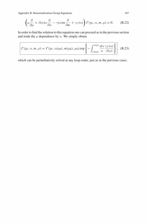
Appendix B: Renormalization Group Equations 187

(μ

∂

∂μ+ β(α)α

∂

∂α− γ(α)m

∂

∂m+ γΓ (α)

)Γ (pi ,α, m,μ) = 0. (B.22)

In order to find the solution to this equation one can proceed as in the previous sectionand trade the μ dependence by α. We simply obtain

Γ (pi ,α, m,μ) = Γ (pi ,α(μ0), m(μ0),μ0) exp

{−

∫ α(μ)

α(μ0)

dα

α

γΓ (α)

β(α)

}, (B.23)

which can be perturbatively solved at any loop-order, just as in the previous cases.

Appendix CFeynman Rules for Derivative Couplings

The formal steps to derive the Feynman rules from the interaction Lagrangian fornormal vertices is straightforward and nicely presented in the literature. Herewe shallonly present a trick, useful to derive the Feynman rules corresponding to vertices thatcontain derivatives of the fields (and correctly assign the corresponding momenta).Consider the Scalar QED interaction Lagrangian given by

L = ieAμ H+←→∂μ H− = ieAμ

(H+∂μH− − (∂μH+)H−)

. (C.1)

We know fromWick’s theorem that H− describes an ingoing particle or an outgoingantiparticle, also that H+ describes an ingoing antiparticle or an outgoing particle.Let’s now consider we want to write down the Feynman rule corresponding to thefollowing process H−(p) → H−(q)γ(p−q) shown in the Feynman diagram below

p

q

H−

H−

Aµ

p− q

As we also know, in momentum space e−i p·x describes an ingoing particle (antipar-ticle) with momentum p and eip·x describes an outgoing particle (antiparticle) withmomentum p. Thus, substituting the fields from the interaction Lagrangian by theircorresponding exponentials, assigning the momenta shown in the previous Feynmandiagram we get

L = ieei(p−q)·x(eiq·x∂μe−i p·x − (∂μeiq·x )e−i p·x)

= e(p + q)μ. (C.2)

© Springer International Publishing Switzerland 2016V. Ilisie, Concepts in Quantum Field Theory,UNITEXT for Physics, DOI 10.1007/978-3-319-22966-9

189

190 Appendix C: Feynman Rules for Derivative Couplings

Multiplying by an i factor (which comes from the S matrix expansion) we obtain thecorresponding Feynman rule for this vertex

ie(p + q)μ . (C.3)

Using the same trick one finds that H+(p) → H+(q)γ(p − q) is given by thefollowing Feynman rule

−ie(p + q)μ . (C.4)

This can be easily extended to any configuration of momenta and to any Lagrangiancontaining termswith derivative couplings. It very usual to find for example Feynmanrules for triple gauge vertices (or similar) i.e., the triple gluon vertex given at the endof Chap.5, where all momenta are incoming (which seems to violate momentumconservation). It is done like that for simplicity. Depending on the assignation ofmomenta for the process that one analyses, one must simply invert the necessarysigns of the momenta to convert particles/antiparticles from incoming to outgoing.

Further Reading

L.H. Ryder, Quantum Field Theory, Cambridge University Press (1985)A. Pich, Effective Field Theory, http://arxiv.org/abs/hep-ph/9806303C. Itzykson, J. Zuber, Quantum Field TheoryA. Pich, Quantum Chromodynamics, http://arxiv.org/pdf/hep-ph/9505231v1.pdfM.E. Peskin, D.V. Schroeder, An Introduction to Quantum Field TheoryT.P. Cheng, L.F. Li, Gauge Theory of Elementary Particle Physics, Oxford (1984)F. Mandl, G.P. Shaw, Quantum Field Theory