Embed Size (px)
Citation preview

XPMPro 2.0 User's Manual
Document version 1.0.0Last modified 11/05 /2008
XPMPro 2.0 User's Manual Table of Contents
Table of ContentsXPMPro User's Manual................................................................................................................1Introduction...................................................................................................................................5Installation.....................................................................................................................................7
Upgrade from SPM32...........................................................................................................10Image processing on additional computers...........................................................................10
Initial Setup..................................................................................................................................11Options..................................................................................................................................12
Stored parameter files..................................................................................................12Scale bar and color scale..............................................................................................12Default Size..................................................................................................................13Graph Settings..............................................................................................................13dataSAFE.....................................................................................................................13
ACQ window........................................................................................................................14DSP tab........................................................................................................................14Gains tab......................................................................................................................16Scanner tab...................................................................................................................17Closed-loop scanning...................................................................................................17Operating Modes..........................................................................................................19Define tab.....................................................................................................................20Scan Settings................................................................................................................21
dataSAFE.................................................................................................................22Input tab.......................................................................................................................22Scan tab........................................................................................................................23ACQ status bar.............................................................................................................25
Coarse Approach.........................................................................................................................26Navigation window...............................................................................................................27
Aux Feedback..............................................................................................................27Spec Location...............................................................................................................28Tip Approach...............................................................................................................28
Tip control tab..........................................................................................................31Advanced approach settings.....................................................................................34Configuring approach motors..................................................................................36
Kinetic approach systems......................................................................................36Stepper motor........................................................................................................38Omicron 8 channel MSCU....................................................................................39Omicron 3 channel microslide controller..............................................................41RHK PMC100.......................................................................................................41Inchworm(TM)/TTL.............................................................................................42Attocube motor......................................................................................................43PPC200 USB controlled piezo positioning controllers.........................................43
Starting an approach.................................................................................................44Tip Track......................................................................................................................45Manual control.............................................................................................................45
RHK Technology 2 Troy, MI, USA
XPMPro 2.0 User's Manual Table of Contents
SPM Status...................................................................................................................46Initial Acquisition........................................................................................................................47
RTAW toolbar......................................................................................................................48Image manipulation and color table dialog...........................................................................49Navigation window...............................................................................................................50XY Graph window................................................................................................................56
Layout tab....................................................................................................................57Curves tab....................................................................................................................58
Point spectroscopy................................................................................................................60Output tab.....................................................................................................................61Ramp subsection..........................................................................................................62Control tab...................................................................................................................63Advanced modes tab....................................................................................................65Time Spectrum tab.......................................................................................................67Point spectroscopy locations........................................................................................69
Spectrum Analyzer...............................................................................................................74Oscilloscope .........................................................................................................................76Alternative Imaging Modes..................................................................................................76
Multiple parameter imaging (MPI)..............................................................................76Automatic parameter incrementing (API)...................................................................79
Analysis and Processing..............................................................................................................82SM4 file format.....................................................................................................................85Interactive histogram equalization........................................................................................88Cursor Modes........................................................................................................................90Data Analysis........................................................................................................................93Processing.............................................................................................................................98
Processing images in Fourier space...........................................................................101Three-dimensional rendering..............................................................................................103Exporting data.....................................................................................................................105
Advanced Techniques...............................................................................................................107Increasing resolution...........................................................................................................110Variable gap spectroscopy..................................................................................................111StabiliDrift..........................................................................................................................112Conductance measurements................................................................................................114
Barrier height measurements using I-z spectroscopy................................................115Barrier height measurements using a lockin amplifier..............................................116Measurement parameters...........................................................................................117
Input/Output line-by-line imaging......................................................................................118Force setpoint when using a commercial AFM..................................................................119
Changing the setpoint force using the setpoint knob.................................................121Changing the setpoint force using the bias knob.......................................................122
Handshaking.......................................................................................................................123Lateral drift correction........................................................................................................124Vertical drift correction......................................................................................................126Tip tracking of a feature......................................................................................................128
RHK Technology 3 Troy, MI, USA

XPMPro 2.0 User's Manual Table of Contents
Forming a panorama view in the NAV window.................................................................129Manipulation and Lithography...........................................................................................129
Appendices.................................................................................................................................133SM4 Data File Format........................................................................................................134DSP Scan Board Commands..............................................................................................149
RHK Technology 4 Troy, MI, USA

XPMPro 2.0 User's Manual Introduction
Introduction
RHK Technology 5 Troy, MI, USA
XPMPro 2.0 User's Manual Introduction
XPMPro 2.0 is a new version of RHK SPM control software. Commonly, it is used to control SPM100 electronics from RHK Technology. It features advanced acquisition capabilities, sophisticated data processing algorithms, and superior manipulation and lithography controls.
This software includes all of the feature gained through 13 years of development on SPM32 and several years of the development on XPMPro. Compare with the XPMPro, it has the following improvements and enhancements:
● Look and Feel. XPMPro™ 2.0 has had a face lift and reorganized controls to make the operation more intuitive, enabling even beginning users to access and utilize the advanced functionality that has made XPMPro the favorite of advanced researchers.
● Dynamic Data Oversampling. When enabled, acquisition boards will run at their maximum sampling rate and average all readings between pixels. At present XPMPro only takes one reading per pixel. Oversampling will yield better S/N, especially when scanning slowly
● Spectroscopic Drift Correction. When enabled, the software will automatically correct for drift in all three axis between multiple spectroscopy curves taken at the same location. At present XPMPro can correct for drift between curves only in the Z axis. Exact location of spectroscopic measurement will be stored with each curve
● Workspace Sessions. This function will save all open windows in the DAW and store them in one file, called a session. When you reopen that session, all windows will return to their original position so you can start where you left off processing and analysis. This session file can also be emailed to collaborators
● Oscilloscope. The maximum number of samples increased from 256k to 1 MS. Data can be acquired while utilizing Drag/Move Tip functions and during Pulse operation. Also settings for using this option have been moved to the oscilloscope window for easier operation
● Time Spec UI implementation. This new spectroscopy acquisition mode allows the user to program an experiment where any two parameters, such as Z position and bias voltage can be ramped between end points at any predefined rate, stay at the end point for a predefined period (dwell time), and then continue to the next set of end points, all the while collecting data on any number of input channels. Ten steps in this process can be programmed to be automatically acquired at any number of points in an image
● Spectrum Analyzer. Settings controls attached with window, and the maximum number of readings has been increased to 8,192k, providing 50 mHz resolution with a bandwidth of 125 kHz. Optional acquisition module provides up to 2 MHz sampling. It displays the average spectrum in real-time, which provides higher speed and resolution. Furthermore, all settings have been moved to the Power Spectrum window for ease of operation.
● Feature Tracking and display. When using the feature tracking capability, the position of the feature on the surface is recorded as a function of time. A new display mode allows this position to be shown as a function of time or displayed overlaid on the image where it was acquired
● Improved Atomic Manipulation. Dropped atomic features during manipulation routines are no longer a problem. RHK has improved upon its previously released design. The updated atomic manipulation routine improves productivity by up to 100 fold by quickly and automatically locating lost features.
RHK Technology 6 Troy, MI, USA
XPMPro 2.0 User's Manual Installation
● High Speed acquisition module. A new optional module allows acquisition to be acquired at up to 2 MHz on each of two channels. In additional to allowing faster imaging, the higher bandwidth can also be utilized by the oscilloscope and spectrum analyzer functions. This module can be added to any existing SPM1000 system running XPMPro Version 2.0.
● Increased scan speeds. The software has been optimized to allow much faster data acquisition. For example, up to twelve images of 128x128 resolution can now be acquired per second (six images in each scan direction).
● Average spectroscopy curves in real time. This function displays the running average of all curves taken at each point in real time in additional to the display of each individual spectroscopy curve.
● Real-time processing and display of spectroscopic data. In addition to showing the raw data for each curve, real-time display of calculated derivative and/or second derivative can also be shown.
● Redesigned Analysis and Processing software. The analysis and processing sections of the software have been upgraded to provide much faster and efficient processing and visualization.
● Integration of PLLPro into XPMPro. Tight integration of the PLLpro into XPMPro greatly improves ease of use.
● PMC100 integration into XPMPro. All configuration functions of PMC100 are now set inside of XPMPro instead of through separate application
Customers upgrading from SPM32 and XPMPro will recognize most of the features and enjoy an easier to use interface through a reorganization of controls as well as a polished GUI made possible by the Windows OS.
RHK Technology 7 Troy, MI, USA

XPMPro 2.0 User's Manual Installation
Installation
RHK Technology 8 Troy, MI, USA
XPMPro 2.0 User's Manual Installation
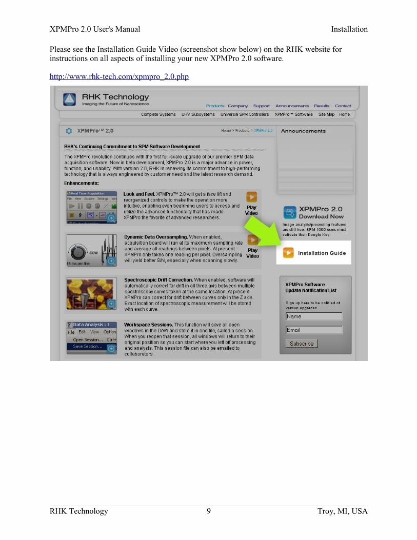
Please see the Installation Guide Video (screenshot show below) on the RHK website for instructions on all aspects of installing your new XPMPro 2.0 software.
http://www.rhk-tech.com/xpmpro_2.0.php
RHK Technology 9 Troy, MI, USA
XPMPro 2.0 User's Manual Initial Setup
Initial Setup
RHK Technology 10 Troy, MI, USA
XPMPro 2.0 User's Manual Initial Setup
When the program is started, it will check for the presence of the sentinel key on the parallel port of the computer This is the same protection key used to authorize SPM32. For existing users, an upgrade password will be required to activate the key for XPMPro If the key has been activated for XPMPro, the program will try to connect to the SPM100. This will fail because the IP address of the SPM100 has not been entered into the software yet. The screen will then display the main tool bar as shown in Figure 1.
OptionsThe OPT menu can also be used to unlock additional features of the software that require an extra password. At this time, the only additional module is the high speed scanning option provided by the Data Translation DT9832 USB adapter. This menu is also used to access some universal parameters that apply to both the acquisition window and the analysis and processing menu.
Stored parameter files
Click the OPT button to open a menu where different parameter files can be opened. The PRM files store all of the settings in the program. The ability to switch PRM files allows multiple systems to be operated from a single installation. Piezo calibrations, stored spectroscopy experiments, etc. are kept in the PRM file and can be individually maintained. Since the new SM4 file format contains the complete PRM file inside its file header, an experiment can be recreated from the stored data file by choosing to read the parameters out of the stored data file. This is accomplished by choosing Read PRM from SM4 file. Note, this is only possible from an SM4 file saved with XPMPro 2.0 and above. An SM4 file converted from an existing SM3 file will not have the parameters stored in it since that feature was not available as part of the SM3 format specification. After choosing this menu option, click on the desired SM4 file in the file browser. An alternative method of importing settings from a saved file is to choose the menu item DAW Page and then click on an open data window in a the DAW. This will retrieve the PRM file from the saved SM4 file associated with this data. The third option for changing parameter files is the traditional way of directly browsing for a different PRM file using the standard file browser. We also can store the working parameter to a prm file at the folder that we want.
Explore folders
Shortcuts to the working folder and support folders are added to the options. The install folder of XPMPro 2.0 can be easily found by these shortcuts. Also the electronic version of the supporting files also can be easily found by these shortcut.
RHK Technology 11 Troy, MI, USA
Figure 1 Screen shot of XPMPro main window
XPMPro 2.0 User's Manual Initial Setup
ACQ window
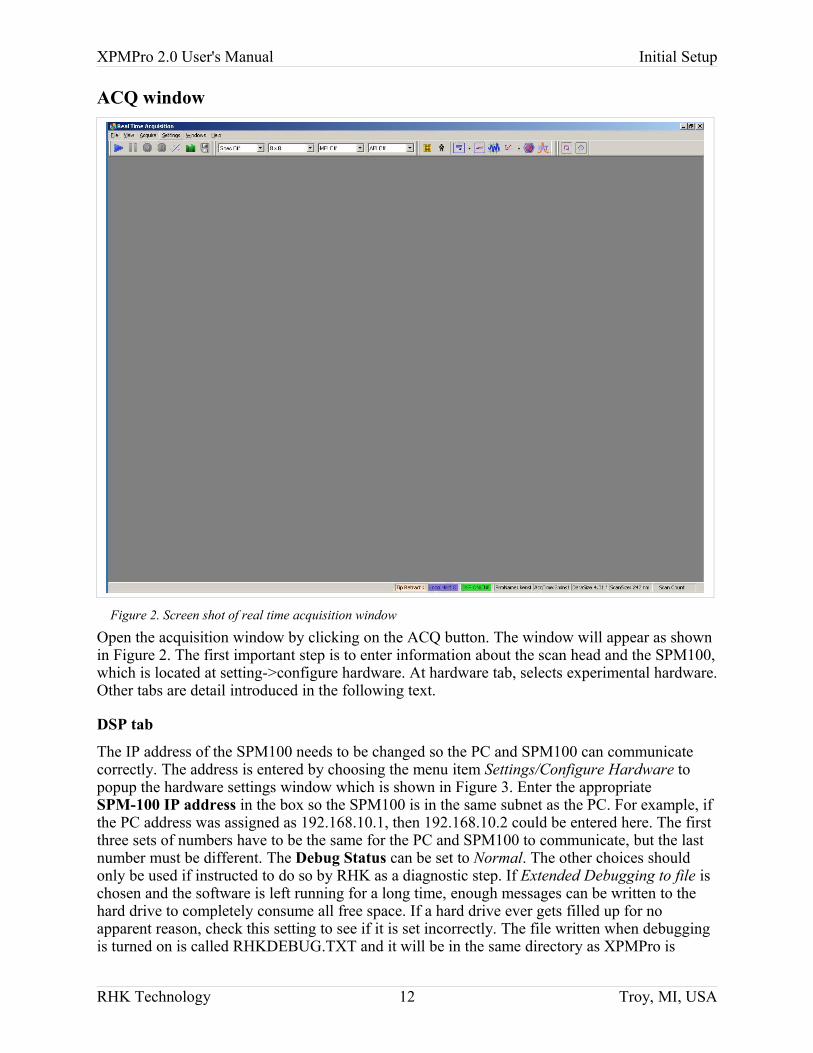
Open the acquisition window by clicking on the ACQ button. The window will appear as shown in Figure 2. The first important step is to enter information about the scan head and the SPM100, which is located at setting->configure hardware. At hardware tab, selects experimental hardware. Other tabs are detail introduced in the following text.
DSP tab
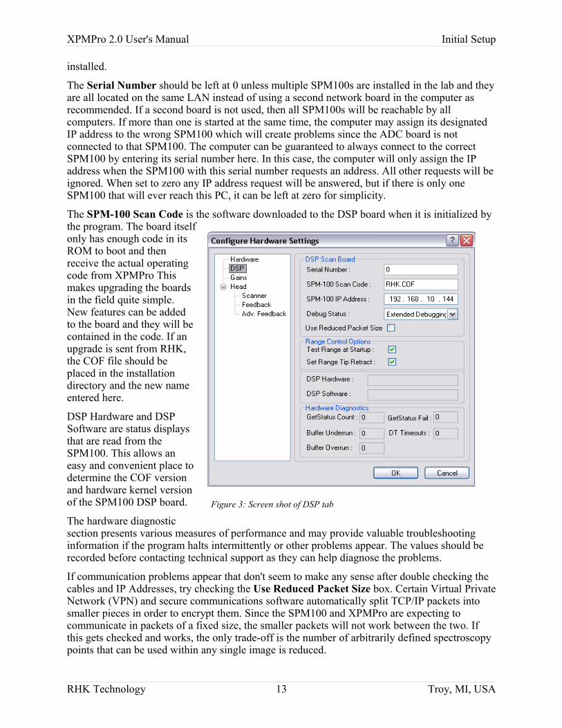
The IP address of the SPM100 needs to be changed so the PC and SPM100 can communicate correctly. The address is entered by choosing the menu item Settings/Configure Hardware to popup the hardware settings window which is shown in Figure 3. Enter the appropriate SPM-100 IP address in the box so the SPM100 is in the same subnet as the PC. For example, if the PC address was assigned as 192.168.10.1, then 192.168.10.2 could be entered here. The first three sets of numbers have to be the same for the PC and SPM100 to communicate, but the last number must be different. The Debug Status can be set to Normal. The other choices should only be used if instructed to do so by RHK as a diagnostic step. If Extended Debugging to file is chosen and the software is left running for a long time, enough messages can be written to the hard drive to completely consume all free space. If a hard drive ever gets filled up for no apparent reason, check this setting to see if it is set incorrectly. The file written when debugging is turned on is called RHKDEBUG.TXT and it will be in the same directory as XPMPro is
RHK Technology 12 Troy, MI, USA
Figure 2. Screen shot of real time acquisition window
XPMPro 2.0 User's Manual Initial Setup
installed.
The Serial Number should be left at 0 unless multiple SPM100s are installed in the lab and they are all located on the same LAN instead of using a second network board in the computer as recommended. If a second board is not used, then all SPM100s will be reachable by all computers. If more than one is started at the same time, the computer may assign its designated IP address to the wrong SPM100 which will create problems since the ADC board is not connected to that SPM100. The computer can be guaranteed to always connect to the correct SPM100 by entering its serial number here. In this case, the computer will only assign the IP address when the SPM100 with this serial number requests an address. All other requests will be ignored. When set to zero any IP address request will be answered, but if there is only one SPM100 that will ever reach this PC, it can be left at zero for simplicity.
The SPM-100 Scan Code is the software downloaded to the DSP board when it is initialized by the program. The board itself only has enough code in its ROM to boot and then receive the actual operating code from XPMPro This makes upgrading the boards in the field quite simple. New features can be added to the board and they will be contained in the code. If an upgrade is sent from RHK, the COF file should be placed in the installation directory and the new name entered here.
DSP Hardware and DSP Software are status displays that are read from the SPM100. This allows an easy and convenient place to determine the COF version and hardware kernel version of the SPM100 DSP board.
The hardware diagnostic section presents various measures of performance and may provide valuable troubleshooting information if the program halts intermittently or other problems appear. The values should be recorded before contacting technical support as they can help diagnose the problems.
If communication problems appear that don't seem to make any sense after double checking the cables and IP Addresses, try checking the Use Reduced Packet Size box. Certain Virtual Private Network (VPN) and secure communications software automatically split TCP/IP packets into smaller pieces in order to encrypt them. Since the SPM100 and XPMPro are expecting to communicate in packets of a fixed size, the smaller packets will not work between the two. If this gets checked and works, the only trade-off is the number of arbitrarily defined spectroscopy points that can be used within any single image is reduced.
RHK Technology 13 Troy, MI, USA
Figure 3: Screen shot of DSP tab

XPMPro 2.0 User's Manual Initial Setup
Gains tab
The preamp gain and high voltage amplifier gains are set in the Gains tab (Figure 4). Internally the signals are all limited to +/- 10 V. To properly calibrate and record all settings, XPMPro must know the physical signal with respect to the internal voltage. The proper conversion factor is entered here. For a high voltage unit where the maximum output is 215 V, the gains should all be set to 21.5. For a low voltage unit, the gains are equal to 13. Other factors are possible depending on the setup of the head. Whatever voltage is applied to the head compared to the internal 10 V signal needs to be entered here. Two other common situations are using the SPM100 with the RHK HVA900 which has a maximum output of 450 V. In this case, the gains are 45. The second is if the optional 0-10 V board is installed which is used to drive a closed loop stage from a third party, the correct value here is 0.5.
Newer SPM100s have the gain of the high voltage outputs programmed into the EEPROM of the unit. If no modifications have been performed to the unit since it left the factory, the Use values stored in SPM100 can be checked. This prevents the gain values from being changed accidentally which would subsequently change the scan head calibration.
Unless the sample bias output from the SPM100 is externally amplified or attenuated, the gain of the bias should always be one. If the bias out put is externally amplified or attenuated, here should be amplification number or attenuated fraction. The STM Current per monitor volt depends on the overall preamplifier gain. A gain of 108 would mean 10 nA/volt. A gain of 109
would mean 1 nA/volt. If this value is entered wrong, then all recorded currents (tunneling conditions, spectroscopy readings, etc.) will be incorrect but can easily be scaled later if the value entered here when the data was acquired is known. If it is easier to think of the current calibration factor in terms of a gain factor, the correct value can also be used in the Preamp gain entry box. This will be the inverse of the setting directly above it and changing one automatically changes the other.
RHK Technology 14 Troy, MI, USA
Figure 4: Screen shot of Gain tab
XPMPro 2.0 User's Manual Initial Setup
Scanner tab
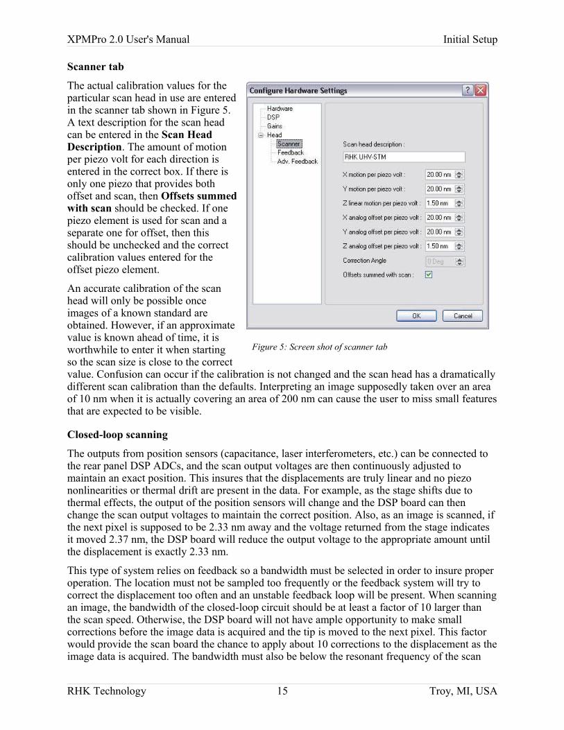
The actual calibration values for the particular scan head in use are entered in the scanner tab shown in Figure 5. A text description for the scan head can be entered in the Scan Head Description. The amount of motion per piezo volt for each direction is entered in the correct box. If there is only one piezo that provides both offset and scan, then Offsets summed with scan should be checked. If one piezo element is used for scan and a separate one for offset, then this should be unchecked and the correct calibration values entered for the offset piezo element.
An accurate calibration of the scan head will only be possible once images of a known standard are obtained. However, if an approximate value is known ahead of time, it is worthwhile to enter it when starting so the scan size is close to the correct value. Confusion can occur if the calibration is not changed and the scan head has a dramatically different scan calibration than the defaults. Interpreting an image supposedly taken over an area of 10 nm when it is actually covering an area of 200 nm can cause the user to miss small features that are expected to be visible.
Closed-loop scanning
The outputs from position sensors (capacitance, laser interferometers, etc.) can be connected to the rear panel DSP ADCs, and the scan output voltages are then continuously adjusted to maintain an exact position. This insures that the displacements are truly linear and no piezo nonlinearities or thermal drift are present in the data. For example, as the stage shifts due to thermal effects, the output of the position sensors will change and the DSP board can then change the scan output voltages to maintain the correct position. Also, as an image is scanned, if the next pixel is supposed to be 2.33 nm away and the voltage returned from the stage indicates it moved 2.37 nm, the DSP board will reduce the output voltage to the appropriate amount until the displacement is exactly 2.33 nm.
This type of system relies on feedback so a bandwidth must be selected in order to insure proper operation. The location must not be sampled too frequently or the feedback system will try to correct the displacement too often and an unstable feedback loop will be present. When scanning an image, the bandwidth of the closed-loop circuit should be at least a factor of 10 larger than the scan speed. Otherwise, the DSP board will not have ample opportunity to make small corrections before the image data is acquired and the tip is moved to the next pixel. This factor would provide the scan board the chance to apply about 10 corrections to the displacement as the image data is acquired. The bandwidth must also be below the resonant frequency of the scan
RHK Technology 15 Troy, MI, USA
Figure 5: Screen shot of scanner tab
XPMPro 2.0 User's Manual Initial Setup
stage or oscillations will occur. Most stages have a fundamental mode of less than a kHz or so. Therefore, many users will have to reduce the image scan speed to take advantage of the closed loop capabilities.
The calibration of the closed loop sensors must be carried out and the appropriate scale factors then entered into the software. A known grating should be scanned and after the features are measured, the known dimensions are compared to the output voltages from the displacement sensors to provide a distance/voltage calibration. The second way to calibrate the position sensors is with the automatic calibration feature. The DSP scan board performs a series of scans with specified dimensions and the output of the sensors measured with the ADC1 and ADC2. Since a known distance was scanned, the sensor output per distance can be calculated and the calibration factors will be automatically entered into the software in the advanced feedback tab. Note that when XPMPro sets up the measurement series, it relies on knowing the position of the front panel X Scan Range knob in order to specify the scan size to the DSP board. The sensor calibration factors are therefore dependent on the X Scan Range knob position. If the range knob is turned (to increase or decrease the available scan area) the automatic calibration routine MUST be performed again.
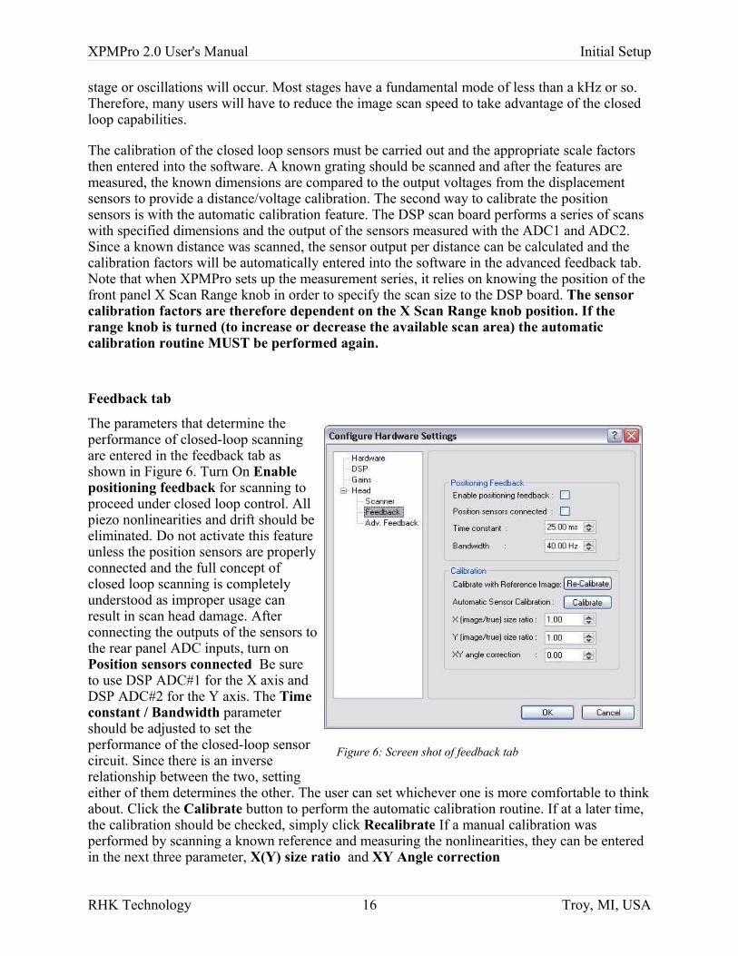
Feedback tab
The parameters that determine the performance of closed-loop scanning are entered in the feedback tab as shown in Figure 6. Turn On Enable positioning feedback for scanning to proceed under closed loop control. All piezo nonlinearities and drift should be eliminated. Do not activate this feature unless the position sensors are properly connected and the full concept of closed loop scanning is completely understood as improper usage can result in scan head damage. After connecting the outputs of the sensors to the rear panel ADC inputs, turn on Position sensors connected Be sure to use DSP ADC#1 for the X axis and DSP ADC#2 for the Y axis. The Time constant / Bandwidth parameter should be adjusted to set the performance of the closed-loop sensor circuit. Since there is an inverse relationship between the two, setting either of them determines the other. The user can set whichever one is more comfortable to think about. Click the Calibrate button to perform the automatic calibration routine. If at a later time, the calibration should be checked, simply click Recalibrate If a manual calibration was performed by scanning a known reference and measuring the nonlinearities, they can be entered in the next three parameter, X(Y) size ratio and XY Angle correction
RHK Technology 16 Troy, MI, USA
Figure 6: Screen shot of feedback tab
XPMPro 2.0 User's Manual Initial Setup
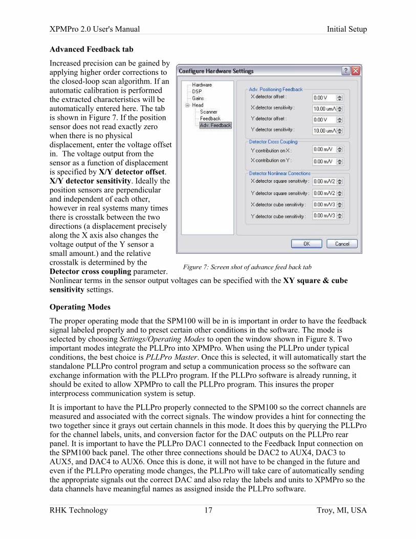
Advanced Feedback tab
Increased precision can be gained by applying higher order corrections to the closed-loop scan algorithm. If an automatic calibration is performed the extracted characteristics will be automatically entered here. The tab is shown in Figure 7. If the position sensor does not read exactly zero when there is no physical displacement, enter the voltage offset in. The voltage output from the sensor as a function of displacement is specified by X/Y detector offset. X/Y detector sensitivity. Ideally the position sensors are perpendicular and independent of each other, however in real systems many times there is crosstalk between the two directions (a displacement precisely along the X axis also changes the voltage output of the Y sensor a small amount.) and the relative crosstalk is determined by the Detector cross coupling parameter. Nonlinear terms in the sensor output voltages can be specified with the XY square & cube sensitivity settings.
Operating Modes
The proper operating mode that the SPM100 will be in is important in order to have the feedback signal labeled properly and to preset certain other conditions in the software. The mode is selected by choosing Settings/Operating Modes to open the window shown in Figure 8. Two important modes integrate the PLLPro into XPMPro. When using the PLLPro under typical conditions, the best choice is PLLPro Master. Once this is selected, it will automatically start the standalone PLLPro control program and setup a communication process so the software can exchange information with the PLLPro program. If the PLLPro software is already running, it should be exited to allow XPMPro to call the PLLPro program. This insures the proper interprocess communication system is setup.
It is important to have the PLLPro properly connected to the SPM100 so the correct channels are measured and associated with the correct signals. The window provides a hint for connecting the two together since it grays out certain channels in this mode. It does this by querying the PLLPro for the channel labels, units, and conversion factor for the DAC outputs on the PLLPro rear panel. It is important to have the PLLPro DAC1 connected to the Feedback Input connection on the SPM100 back panel. The other three connections should be DAC2 to AUX4, DAC3 to AUX5, and DAC4 to AUX6. Once this is done, it will not have to be changed in the future and even if the PLLPro operating mode changes, the PLLPro will take care of automatically sending the appropriate signals out the correct DAC and also relay the labels and units to XPMPro so the data channels have meaningful names as assigned inside the PLLPro software.
RHK Technology 17 Troy, MI, USA
Figure 7: Screen shot of advance feed back tab
XPMPro 2.0 User's Manual Initial Setup
The other entry named PLLPro User will not gray out any of the entries and is intended to be used by advanced users who have setup the PLLPro to operate in a mode that is not straightforward and requires manually entering the channel labels and units. XPMPro will still gather status data and measure the signals from the PLLPro, but the physical interpretation and connections between the two units have to be configured manually.
Define tab
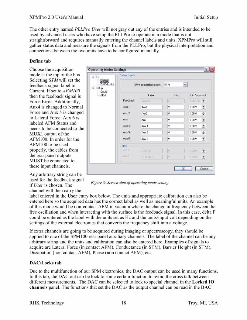
Choose the acquisition mode at the top of the box. Selecting STM will set the feedback signal label to Current. If set to AFM100 then the feedback signal is Force Error. Additionally, Aux4 is changed to Normal Force and Aux 5 is changed to Lateral Force. Aux 6 is labeled AFM Status and needs to be connected to the MUX1 output of the AFM100. In order for the AFM100 to be used properly, the cables from the rear panel outputs MUST be connected to these input channels.
Any arbitrary string can be used for the feedback signal if User is chosen. The channel will then carry the label entered in the User entry box below. The units and appropriate calibration can also be entered here so the acquired data has the correct label as well as meaningful units. An example of this mode would be non-contact AFM in vacuum where the change in frequency between the free oscillation and when interacting with the surface is the feedback signal. In this case, delta F could be entered as the label with the units set as Hz and the units/input volt depending on the settings of the external electronics that converts the frequency shift into a voltage.
If extra channels are going to be acquired during imaging or spectroscopy, they should be applied to one of the SPM100 rear panel auxiliary channels. The label of the channel can be any arbitrary string and the units and calibration can also be entered here. Examples of signals to acquire are Lateral Force (in contact AFM), Conductance (in STM), Barrier Height (in STM), Dissipation (non contact AFM), Phase (non contact AFM), etc.
DAC/Locks tab
Due to the multifunction of our SPM electronics, the DAC output can be used in many functions. In this tab, the DAC out can be lock to some certain function to avoid the cross talk between different measurements. The DAC can be selected to lock to special channel in the Locked IO channels panel. The functions that set the DAC as the output channel can be read in the DAC
RHK Technology 18 Troy, MI, USA
Figure 8: Screen shot of operating mode setting
XPMPro 2.0 User's Manual Initial Setup
assignment panel.
Count tab and AFM tab
Some of user may use the counter to count the photon or electron for the measurement. The setting of the counter can be set at count tab. The main parameters are the count interval and some display parameters.
When we use AFM mode, AFM detector parameters are set here. They are vertical force spring constant, deflection sensitivity, lateral force constant, lateral deflection sensitivity, laser current gain, laser photocurrent gain, PSD thresh hold, or some external signal parameters. (given the typical value of these parameters)
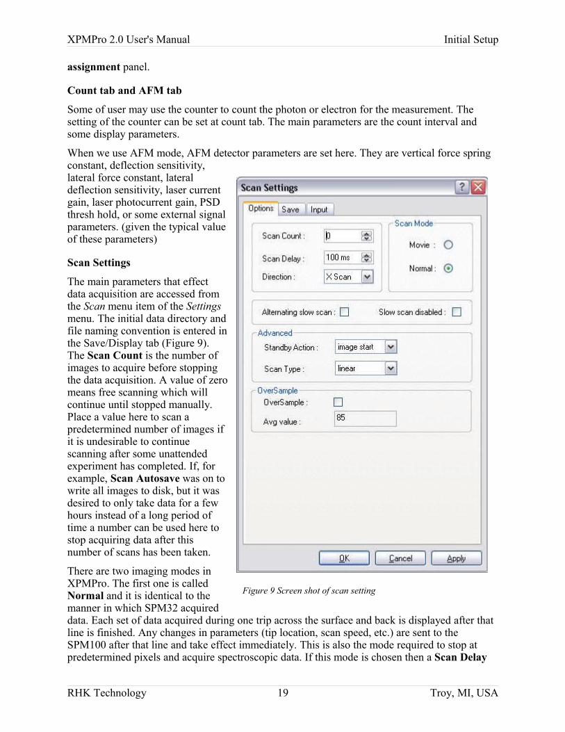
Scan Settings
The main parameters that effect data acquisition are accessed from the Scan menu item of the Settings menu. The initial data directory and file naming convention is entered in the Save/Display tab (Figure 9). The Scan Count is the number of images to acquire before stopping the data acquisition. A value of zero means free scanning which will continue until stopped manually. Place a value here to scan a predetermined number of images if it is undesirable to continue scanning after some unattended experiment has completed. If, for example, Scan Autosave was on to write all images to disk, but it was desired to only take data for a few hours instead of a long period of time a number can be used here to stop acquiring data after this number of scans has been taken.
There are two imaging modes in XPMPro. The first one is called Normal and it is identical to the manner in which SPM32 acquired data. Each set of data acquired during one trip across the surface and back is displayed after that line is finished. Any changes in parameters (tip location, scan speed, etc.) are sent to the SPM100 after that line and take effect immediately. This is also the mode required to stop at predetermined pixels and acquire spectroscopic data. If this mode is chosen then a Scan Delay
RHK Technology 19 Troy, MI, USA
Figure 9 Screen shot of scan setting
XPMPro 2.0 User's Manual Initial Setup
will occur at the end of the frame before the next frame starts. If the tip needs to quickly return from the bottom of the frame to the top of the frame, this delay allows piezo creep to decay so the first few lines of the subsequent frame do not show distortion. Another useful feature of this delay is when acquiring an automated series of images in unattended mode. The delay can be used to allow a large amount of time to elapse before the next image is acquired in order to give the system plenty of time to reach a new equilibrium or have some slow process occur while capturing a “before” and “after” image. Movie mode simply takes the data as rapidly as possible with no stopping between lines to update parameters etc. It also prevents stopping the scan in the middle of a line to perform spectroscopy measurements. It is most useful if an experiment requires the maximum possible data acquisition rate in order to capture dynamic processes occurring on a short time scale. There is also no pause at the end of the frame to update the entire screen, instead data acquisition keeps going in the background and the data will be displayed when the computer is ready to update the screen for the next image. The overall difference in acquisition rate can be dramatic. If scanning a 128x128 pixel image at 1 ms/line, normal mode could acquire about 2 frames/second Movie mode, on the other hand, could acquire closer to 7 frames/second.
The Direction is used to choose whether scanning occurs along the x axis or y axis. This can also be changed using either the F7 key or pressing the toolbar button on the acquisition window.
An alternative method to prevent creep from distorting the first few lines of an image after the tip is rapidly returned to the upper right corner of the scan frame is to start the next frame from the end point of the last frame. This means an image will be acquired from the top of the frame to the bottom and the next frame will be acquired from the bottom of the image to the top. Place a check in Alternating Slow Scan to use this feature. To obtain a series of scans over the exact same part of the surface (ignoring thermal drift effects), Slow scan disabled should be checked. This can be useful to acquire data for comparison within the same image while changing some external parameter (such as AFM load) or to use as a diagnostic when first setting up image acquisition while optimizing the feedback conditions.
The Standby Action is used to select what the scan head should do when image acquisition is not taking place. The options are to be at rest in the upper right corner of the scan frame, to be at rest at the center of the scan frame, to be at rest at the center of the piezo range, continuous scanning of the first line or continuous scanning of the entire frame. Piezo creep can be minimized if the scan piezo is always in motion repeatedly scanning over the same part of the surface since there is no time when it is at rest and therefore “relaxes”. Choosing scanner zero can be helpful with the RHK UHV350 AFM since the PPC150 can be switched from one direction to another with no adverse effects. If the voltage to the scan head legs is zero and they have no deflection, there will be no abrupt jerk of the head when the PPC150 is switched.
If a scan head is in use that has a resonant frequency which gets excited by the harmonics of the conventional triangular waveform, this can be avoided by changing the Scan Type to sinusoidal instead of linear. Now the scan head decelerates as it approaches the end of the line and accelerates gently after turnaround. This avoids transients in the scan head which could cause it to “ring” after abruptly stopping and turning around to move in the other direction.
To reduce noise multiple ADC readings can be averaged together and the result then be considered the value for that pixel. To activate this feature click the Oversampling checkbox in the window. The slower the line time, the more averages that can be acquired before the next pixel location is reached. As the Line Time or Scan Speed is changed, the number of samples
RHK Technology 20 Troy, MI, USA
XPMPro 2.0 User's Manual Initial Setup
will be automatically updated in the information box. A maximum of 1024 readings can be averaged together. Once this value is reached, slowing the scan down more does not reduce the noise further.
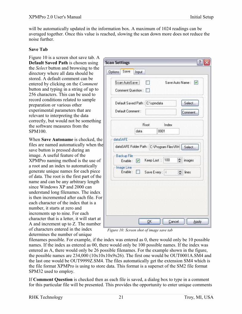
Save Tab
Figure 10 is a screen shot save tab. A Default Saved Path is chosen using the Select button and browsing to the directory where all data should be stored. A default comment can be entered by clicking on the Comment button and typing in a string of up to 256 characters. This can be used to record conditions related to sample preparation or various other experimental parameters that are relevant to interpreting the data correctly, but would not be something the software measures from the SPM100.
When Save Autoname is checked, the files are named automatically when the save button is pressed during an image. A useful feature of the XPMPro naming method is the use of a root and an index to automatically generate unique names for each piece of data. The root is the first part of the name and can be any arbitrary length since Windows XP and 2000 can understand long filenames. The index is then incremented after each file. For each character of the index that is a number, it starts at zero and increments up to nine. For each character that is a letter, it will start at A and increment up to Z. The number of characters entered in the index determines the number of unique filenames possible. For example, if the index was entered as 0, there would only be 10 possible names. If the index as entered as 00, there would only be 100 possible names. If the index was entered as A, there would only be 26 possible filenames. For the example shown in the figure, the possible names are 234,000 (10x10x10x9x26). The first one would be OUT0001A.SM4 and the last one would be OUT9999Z.SM4. The files automatically get the extension SM4 which is the file format XPMPro is using to store data. This format is a superset of the SM2 file format SPM32 used to employ.
If Comment Question is checked then as each file is saved, a dialog box to type in a comment for this particular file will be presented. This provides the opportunity to enter unique comments
RHK Technology 21 Troy, MI, USA
Figure 10: Screen shot of image save tab
XPMPro 2.0 User's Manual Initial Setup
for each file when desirable. Be careful about having this checked though because saving will be halted until the dialog is filled in. Do not activate this and expect to automatically save data in an unattended manner.
It is possible to automatically save every scan acquired without user intervention. Placing a check mark in the Scan Autosave box will save each file to the hard drive with the proper name as determined by the root and index. This feature allows a long series of related images to be saved in unattended fashion.
At the end of each image scan, the color mapping of z values to colors can be adjusted to best fit the data. Activate this feature by checking Autoscale Image. Occasionally this may cause the color map to be worse than before if a single spike is present in the data that skews the maximum z value far from the rest of the data. If this is unchecked then the remapping will only occur when manually requested via the F5 button or the Autoscale button on the toolbar.
In customary GUI standards, the Apply button will save the parameters to the PRM file and have them take effect but leave the window open. The OK button will save the parameters to the PRM file and have them take effect while also closing the window.
dataSAFE
A revolutionary new feature of XPMPro is the ability to periodically save a scan during the acquisition to prevent loss of important data in case of a power outage. The user can choose where to store the temporary files with the Temp Folder Path parameter. To recover a partial scan, the data analysis window can be opened and the temp folder browsed to locate the temp files. Each one is saved with a unique name generated by the date, time, and extra numerical string. All valid data will be displayed as normal and the values for the region of the scan not completed yet are set to zero so that part of the image will look completely flat. The periodic saving is active under two conditions. If the Enable check box in the Line section is checked and if the total acquisition time for the scan exceeds five minutes. The frequency to save data is entered next to the check box by specifying how many lines of data to acquire before writing the file. This is great protection from power failures; after all, a partial piece of important data is better than losing the entire scan.
Be sure to understand the difference between the ring buffer and Scan Autosave. If the second one is checked, then every file is written to the current save path using the filename formed by the root and index parameters and will never be overwritten by XPMPro. If Scan Autosave is not on but the image dataSAFE check box is marked then the complete scan will still be saved to the temp path and can be recovered until overwritten. By using the DAW file browser, any file can be transferred to the save directory by right clicking on the name and choosing Move File. This will be covered in more detail later.
Input tab
To select which channels should be acquired during a scan across the surface, the Input tab (Figure 11) is used. Any channel that has a check mark in the Image column will be sampled at each pixel to form an image. Note that the names of the channels will be whatever was entered in the Operating Modes/Define tab discussed above. If an experiment is taking place where it is desirable to record a signal that does not vary any during the time scale of the scan, then the check box in the Status column should be checked. When this is done the channel is measured once at the end of the scan frame and the data is stored in the file header for a permanent record of the signal level during the image. The most common example of this would be to record the
RHK Technology 22 Troy, MI, USA

XPMPro 2.0 User's Manual Initial Setup
analog output of a temperature meter so the actual temperature is recorded for that data set. There is no need to form a a two dimensional image of temperature because it varies so slowly, the same value would be recorded at nearly every pixel. The voltage can later be displayed using the Page Info command discussed in a later chapter.
The pixel resolution is also selected here. The Ganged button can be checked to acquire images with an equal amount of pixels and lines. In this case, only the Points per line can be selected and Lines per Frame is automatically set to the equal value. If separate is checked, then the Points per Line and Lines per Frame can be chosen independently. Both values are restricted to numbers that are a power of two and range from 8x8 to 8192x8192.
Record one scan direction should be checked if the data is only needed during the forward scan across the surface. This can save time and file size by eliminating data pages and also the amount of time it requires to take data while moving across the surface in some circumstances.
The ADC gain is set for each channel in software. The DT3016 board has programmable gain that can acquire 16 bit resolution data and have it spread over a 20 volt range (0.305 mV LSB) or as small as 2.5 volt (0.0381 mV LSB). When the range is turned down, this increases total sensitivity to provide effectively 19 bits of resolution for all channels except Topography. The total sensitivity for that channel has additional gain from the SPM100 Z Position Gain knob which amplifies the signal before it is sent to the DT3016 board. If the Z Position Gain knob is at 128 and the signal is still very small, increased sensitivity to small corrugation can be obtained by increasing the gain on the ADC board through software using this panel.
To obtain better resolution on the other channels, the gain should be increased until it reaches a point where the signal would saturate the ADC. For example, if a tunneling current of 100 pA is in use, this corresponds to 100 mV signal (assuming 109 gain). Since the signal will rarely exceed even 1 volt (1 nA) the range of the current channel could be changed to +/- 1.25 V so it is
RHK Technology 23 Troy, MI, USA
Figure 11:Screen shot of input tab for scan setting
XPMPro 2.0 User's Manual Initial Setup
possible to detect variations in current with better resolution.
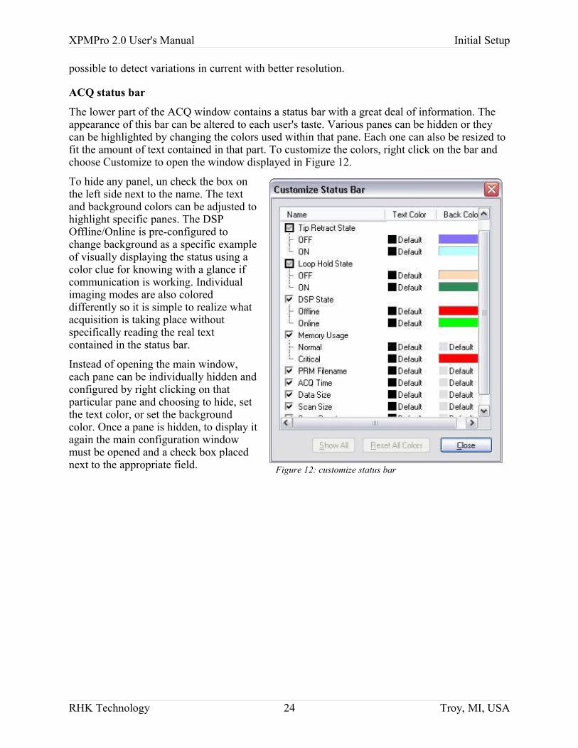
ACQ status bar
The lower part of the ACQ window contains a status bar with a great deal of information. The appearance of this bar can be altered to each user's taste. Various panes can be hidden or they can be highlighted by changing the colors used within that pane. Each one can also be resized to fit the amount of text contained in that part. To customize the colors, right click on the bar and choose Customize to open the window displayed in Figure 12.
To hide any panel, un check the box on the left side next to the name. The text and background colors can be adjusted to highlight specific panes. The DSP Offline/Online is pre-configured to change background as a specific example of visually displaying the status using a color clue for knowing with a glance if communication is working. Individual imaging modes are also colored differently so it is simple to realize what acquisition is taking place without specifically reading the real text contained in the status bar.
Instead of opening the main window, each pane can be individually hidden and configured by right clicking on that particular pane and choosing to hide, set the text color, or set the background color. Once a pane is hidden, to display it again the main configuration window must be opened and a check box placed next to the appropriate field.
RHK Technology 24 Troy, MI, USA
Figure 12: customize status bar

XPMPro User's Manual Coarse Approach
Coarse Approach
RHK Technology 25 Troy, MI, USA
XPMPro User's Manual Coarse Approach
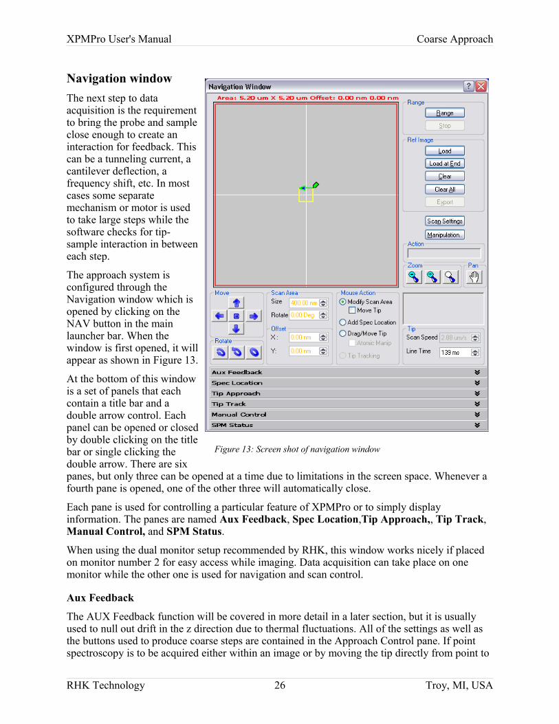
Navigation windowThe next step to data acquisition is the requirement to bring the probe and sample close enough to create an interaction for feedback. This can be a tunneling current, a cantilever deflection, a frequency shift, etc. In most cases some separate mechanism or motor is used to take large steps while the software checks for tip-sample interaction in between each step.
The approach system is configured through the Navigation window which is opened by clicking on the NAV button in the main launcher bar. When the window is first opened, it will appear as shown in Figure 13.
At the bottom of this window is a set of panels that each contain a title bar and a double arrow control. Each panel can be opened or closed by double clicking on the title bar or single clicking the double arrow. There are six panes, but only three can be opened at a time due to limitations in the screen space. Whenever a fourth pane is opened, one of the other three will automatically close.
Each pane is used for controlling a particular feature of XPMPro or to simply display information. The panes are named Aux Feedback, Spec Location,Tip Approach,, Tip Track, Manual Control, and SPM Status.
When using the dual monitor setup recommended by RHK, this window works nicely if placed on monitor number 2 for easy access while imaging. Data acquisition can take place on one monitor while the other one is used for navigation and scan control.
Aux Feedback
The AUX Feedback function will be covered in more detail in a later section, but it is usually used to null out drift in the z direction due to thermal fluctuations. All of the settings as well as the buttons used to produce coarse steps are contained in the Approach Control pane. If point spectroscopy is to be acquired either within an image or by moving the tip directly from point to
RHK Technology 26 Troy, MI, USA
Figure 13: Screen shot of navigation window
XPMPro User's Manual Coarse Approach
point, the locations can be defined using the Spec Location tab. This tool will be described in more detail in a later section. The Tip Tracking pane can be used to configure a lateral dither of the tip over a feature using the X and Y scan raster DACs. The DSP board will then monitor the fluctuations of a signal and by measuring the local gradient it can adjust the center position of the tip to stay above a feature on the surface. This is particularly useful to track diffusion of adsorbates or defects on the surface as well as provide a measure of drift as a function of time. The final pane is a display of all analog signal levels in the SPM100 as well as the two pulse counting channels. This is updated at a rate of approximately three times per second. A large number f readings are measured and averaged together to reduce the jitter in the readings.
Spec Location
Spec Location will be explained in great detail in a later section. It is used to select pixels within an image to stop the scan and acquire spectroscopic data.
Tip Approach
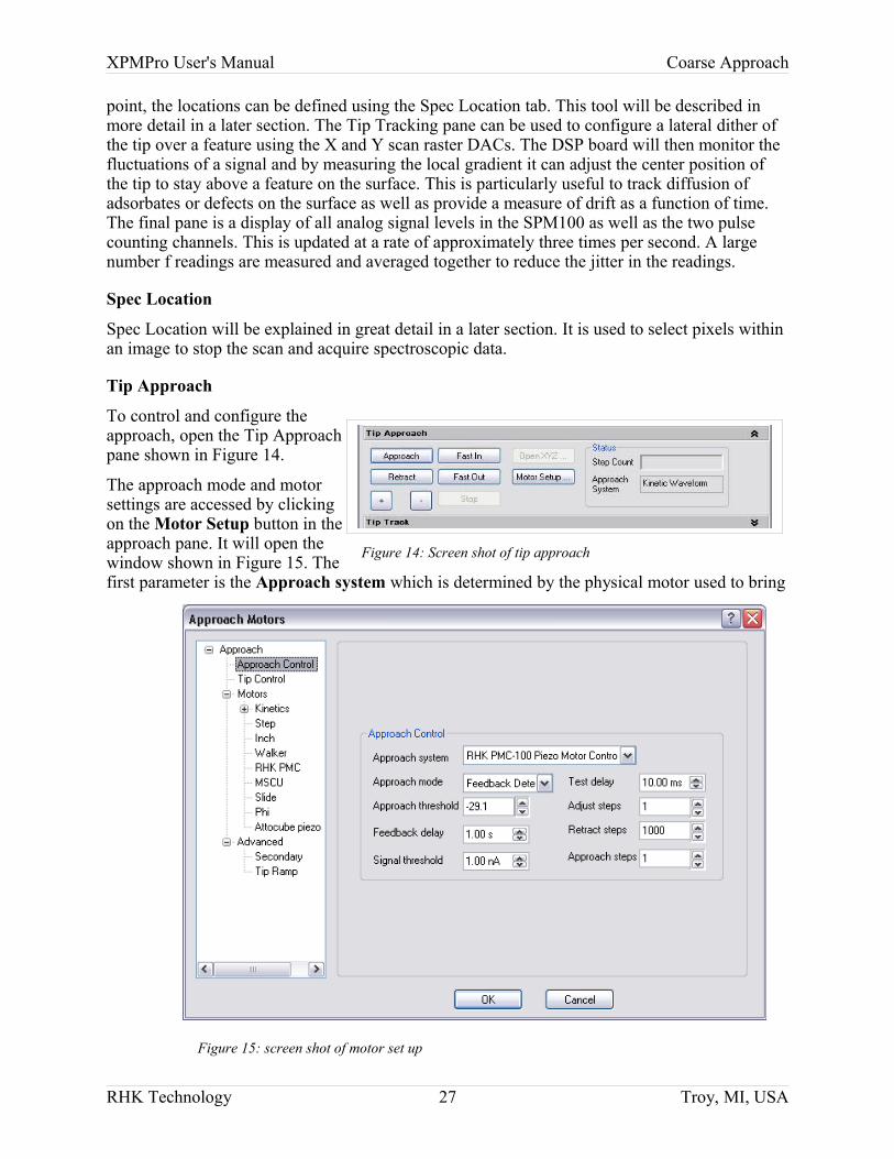
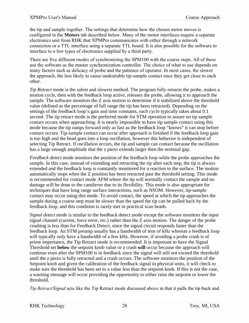
To control and configure the approach, open the Tip Approach pane shown in Figure 14.
The approach mode and motor settings are accessed by clicking on the Motor Setup button in the approach pane. It will open the window shown in Figure 15. The first parameter is the Approach system which is determined by the physical motor used to bring
RHK Technology 27 Troy, MI, USA
Figure 15: screen shot of motor set up
Figure 14: Screen shot of tip approach
XPMPro User's Manual Coarse Approach
the tip and sample together. The settings that determine how the chosen motor moves is configured in the Motors tab described below. Many of the motor interfaces require a separate electronics unit from RHK that XPMPro communicates with either through a network connection or a TTL interface using a separate TTL board. It is also possible for the software to interface to a few types of electronics supplied by a third party.
There are five different modes of synchronizing the SPM100 with the coarse steps. All of these use the software as the master synchronization controller. The choice of what to use depends on many factors such as delicacy of probe and the patience of operator. In most cases, the slower the approach, the less likely to cause undesirable tip-sample contact once they get close to each other.
Tip Retract mode is the safest and slowest method. The program fully retracts the probe, makes a motion cycle, then with the feedback loop active, releases the probe, allowing it to approach the sample. The software monitors the Z axis motion to determine if it stabilized above the threshold value (defined as the percentage of full range the tip has been retracted). Depending on the settings of the feedback loop’s gain and time constants, each cycle typically takes about 0.1 second. The tip retract mode is the preferred mode for STM operation to assure no tip sample contact occurs when approaching. It is nearly impossible to have tip sample contact using this mode because the tip ramps forward only as fast as the feedback loop “knows” it can stop before contact occurs. Tip-sample contact can occur after approach is finished if the feedback loop gain is too high and the head goes into a loop oscillation, however this behavior is independent of selecting Tip Retract. If oscillation occurs, the tip and sample can contact because the oscillation has a large enough amplitude that the z piezo extends larger then the nominal gap.
Feedback detect mode monitors the position of the feedback loop while the probe approaches the sample. In this case, instead of extending and retracting the tip after each step, the tip is always extended and the feedback loop is constantly monitored for a reaction to the surface. The motion automatically stops when the Z position has been retracted past the threshold setting. This mode is recommended for contact mode AFM where the tip will normally contact the sample and no damage will be done to the cantilever due to its flexibility. This mode is also appropriate for techniques that have long range surface interactions, such as NSOM. However, tip-sample contact may occur using this mode. To avoid contact, the speed at which the tip approaches the sample during a coarse step must be slower than the speed the tip can be pulled back by the feedback loop, and this condition is rarely met in practical scan heads.
Signal detect mode is similar to the feedback detect mode except the software monitors the input signal channel (current, force error, etc.) rather than the Z axis motion. The danger of the probe crashing is less than for Feedback Detect, since the signal circuit responds faster than the feedback loop. An STM preamp usually has a bandwidth of tens of kHz whereas a feedback loop will typically only have a bandwidth of a few kHz. However, if avoiding a probe crash is of prime importance, the Tip Retract mode is recommended. It is important to have the Signal Threshold set below the setpoint knob value or a crash will occur because the approach will continue even after the SPM100 is in feedback since the signal will still not exceed the threshold until the z piezo is fully retracted and a crash occurs. The software monitors the position of the Setpoint knob and given the calibration of the feedback signal in physical units, it will check to make sure the threshold has been set to a value less than the setpoint knob. If this is not the case, a warning message will occur providing the opportunity to either raise the setpoint or lower the threshold.
Tip Retract/Signal acts like the Tip Retract mode discussed above in that it pulls the tip back and
RHK Technology 28 Troy, MI, USA
XPMPro User's Manual Coarse Approach
ramps the tip forward using the feedback loop of the SPM100 but instead of monitoring the Z position level, it monitors the feedback channel and stops the approach if the level gets above a threshold. It uses the same Signal Threshold parameter as the Signal Detect method.
Open Loop Ramp takes advantage of the fact that the bandwidth of most preamplifiers is larger than the bandwidth of the feedback loop. Therefore, decreased approach times can be achieved with this method. The feedback electronics of the SPM 100 is bypassed and the tip is ramped towards the sample through direct control using the DT3016 card. The z piezo is ramped forward very quickly between coarse motion steps, and the feedback channel is monitored for a non-zero signal. The response time will depend on the bandwidth of the signal circuit. For STM, the response can easily be as fast as 20 ms (50 kHz bandwidth setting of the IVP-PGA). When the signal goes over a preset threshold indicating a response to the surface has been detected, the ramp is stopped. The tip is then retracted and reapproached at a decreased speed to establish feedback. Since the tip is ramped using the DT3016 card instead of the feedback loop, the amount of time to extend/contract the z piezo between coarse steps is much shorter and the total approach time is much less compared to using the feedback loop of the SPM100 to extend/contract. An output ramp voltage is generated by the ADC card and applied to the appropriate rear panel DAC output of the SPM 100. This BNC is attached to Z position modulation input #1 and the waveform is then amplified and applied directly to the z piezo. The ramp speeds and motion limits are set in the Advanced/Tip Ramp tab discussed below.
The rest of the parameters in this tab set the level when an approach should be considered done as well as the timing and speed. The Approach Threshold is used during a Tip Retract or Feedback Detect approach. The probe is advanced until the control loop stabilizes above the threshold value. The range is -100% to +100%, where -100% is fully extended, and +100% is fully retracted. A value of 0% would mean the probe advances until it is just past the midpoint of the feedback range. Initially, this value should be set to something conservative like -50%. After measuring the step size of the coarse approach relative to the total range of the Z piezo, this can be set to something close to 0% to avoid manual adjustment (via the ‘+’ and ‘-‘ buttons) after coarse approach in order to center the z piezo within its range. The smaller the coarse step size relative to the total z piezo range, the closer this can be used to automatically center the z piezo in its range when an approach is finished. If the coarse step size is close to the total z range then this should be set to a large negative number to avoid taking one extra step which would cause tip-sample contact if the z piezo has run out of range after that step.
When using Feedback detect or Tip Retract mode, Feedback delay sets the amount of time to test if the position of the z piezo is above the threshold value. If the signal remains above the threshold after this amount of time, the controller stops the approach and assumes it is complete. As the feedback loop response time is lowered, this value should be set higher since the SPM 100 will require more time to extend the tip past the threshold while probing for the surface if Tip Retract is used. Values as high as 5 sec. may be needed when the feedback loop is set very low as typically used in NSOM. If the approach stops after a single step but the SPM100 still shows no feedback signal, then this value needs to be increased in order to give the feedback loop a longer time to extend the z piezo past the threshold.
When Signal detect is chosen, the approach continues until the feedback signal is above the Signal Threshold. The parameter can be set to any value within the input range of the feedback signal. When using a STM preamplifier with a gain of 100mV/nA, the maximum value that the feedback current can be set to is 10 nA. A typical value for this is 100 pA. As mentioned above, ALWAYS make sure this value is BELOW the set point knob value or the approach will continue until the tip is fully retracted and then a crash occurs. Be careful not to set it too low or
RHK Technology 29 Troy, MI, USA

XPMPro User's Manual Coarse Approach
noise in the signal may be large enough to cross the threshold which would cause the approach to stop prematurely. Since the software can read the value of the setpoint knob on the front panel of the SPM100, a warning message will be produced if the threshold is set above the knob value.
For Signal test or Feedback detect modes, the Test delay is used to allow a specified amount of time to elapse in case the head is “ringing” due to transients introduced by taking a coarse step. The feedback signal may have large spikes above the threshold which would cause a false engage if the signal was read before the spike decayed.
For approach types that use discrete steps, such as stepper motors, kinetic slip-stick, inchworm, etc., Approach steps determines the number of steps between in-range tests. An in range test should be made between a series of steps that cover between 10-30% of the range of the z piezo motion. If you have a motor that makes very small steps, you can significantly decrease the approach time by increasing this number since there is no need to test for tip-sample interaction between each minuscule step. Theoretically, the approach time will scale linearly with increasing this number. If it only tests every ten coarse steps, the approach should be ten times faster compared to testing after every step. Similarly, Adjust Steps is equal to the number of steps that will be made each time the ‘+’ or ‘-’ buttons in the navigation window are clicked. A typical value would be one but larger motion can be initiated for each button press by using a larger number. When ready to move the tip and sample far apart (for sample change, tip change, etc.), pressing the Retract button will cause the motor to move the number of steps specified by the Retract steps parameter.
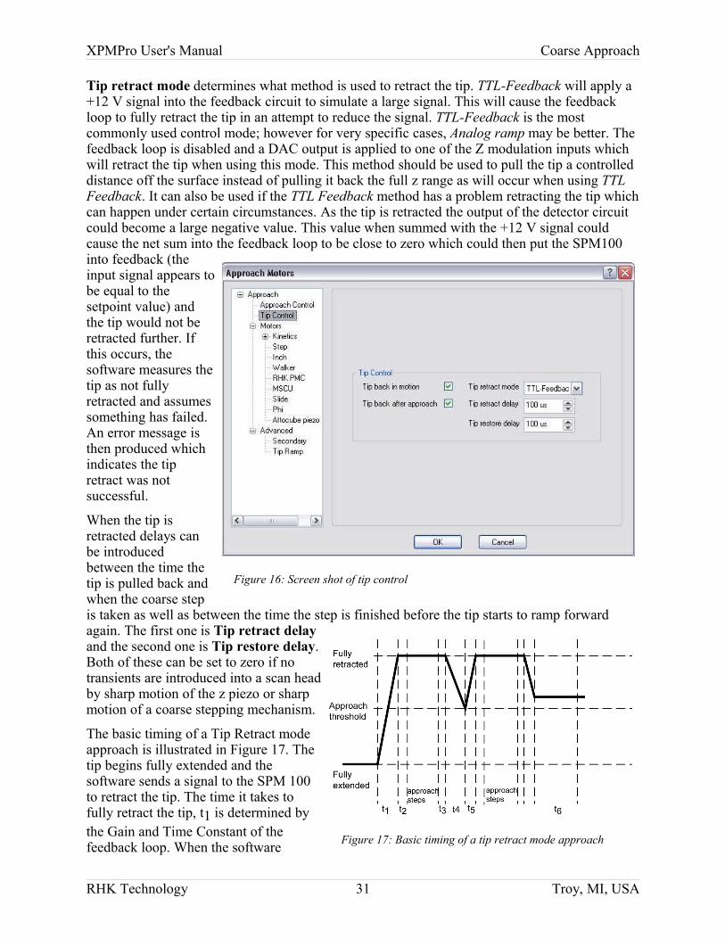
Tip control tab
Helpful choices for tip behavior are contained in the Tip Control tab of the same window (Figure 16). Tip back in motion is the option that determines if the probe should be automatically retracted whenever the software is about to move the probe in any direction using a coarse step. This option should always be set to YES when used with an STM as an extra precaution when trying to avoid tip damage. If the system is used with an AFM that can only move in the Z direction under software control, this parameter can be safely set to NO as long as each approach step will not cause damage to the probe if the feedback loop is slow to respond. If each step in the z direction is large enough and rapid enough that a brittle cantilever could snap, the tip should also be pulled back before taking the step. If motion can be taken laterally than it would be a good idea to pull the tip back before making a large sideways step.
After an approach has finished, the tip can be left at its fully retracted position as an extra precaution against tip damage through accidental tip-surface contact. Many times, an approach can take a very long time and will be performed unattended. However, once the approach is done the tip is in range and very close to the surface. Accidental contact could occur if an isolation table is bumped or someone is unaware an experiment is taking place. By checking Tip back after approach, when the coarse approach is finished the final part of the sequence will be to fully retract the tip the maximum allowed z range and hold this position until it is released by the user through the software. This can be done right away when dismissing the “approach done” dialog or at a later time by unchecking Withdraw Tip in the Manual Control section described later.
RHK Technology 30 Troy, MI, USA
XPMPro User's Manual Coarse Approach
Tip retract mode determines what method is used to retract the tip. TTL-Feedback will apply a +12 V signal into the feedback circuit to simulate a large signal. This will cause the feedback loop to fully retract the tip in an attempt to reduce the signal. TTL-Feedback is the most commonly used control mode; however for very specific cases, Analog ramp may be better. The feedback loop is disabled and a DAC output is applied to one of the Z modulation inputs which will retract the tip when using this mode. This method should be used to pull the tip a controlled distance off the surface instead of pulling it back the full z range as will occur when using TTL Feedback. It can also be used if the TTL Feedback method has a problem retracting the tip which can happen under certain circumstances. As the tip is retracted the output of the detector circuit could become a large negative value. This value when summed with the +12 V signal could cause the net sum into the feedback loop to be close to zero which could then put the SPM100 into feedback (the input signal appears to be equal to the setpoint value) and the tip would not be retracted further. If this occurs, the software measures the tip as not fully retracted and assumes something has failed. An error message is then produced which indicates the tip retract was not successful.
When the tip is retracted delays can be introduced between the time the tip is pulled back and when the coarse step is taken as well as between the time the step is finished before the tip starts to ramp forward again. The first one is Tip retract delay and the second one is Tip restore delay. Both of these can be set to zero if no transients are introduced into a scan head by sharp motion of the z piezo or sharp motion of a coarse stepping mechanism.
The basic timing of a Tip Retract mode approach is illustrated in Figure 17. The tip begins fully extended and the software sends a signal to the SPM 100 to retract the tip. The time it takes to fully retract the tip, t1 is determined by the Gain and Time Constant of the feedback loop. When the software
RHK Technology 31 Troy, MI, USA
Figure 16: Screen shot of tip control
Figure 17: Basic timing of a tip retract mode approach
XPMPro User's Manual Coarse Approach
detects the tip is fully retracted, it waits time t2 the Tip Retract Delay. Then the software performs whatever is necessary to take the requested number of coarse steps (Approach Steps). The amount of time needed here will vary widely depending on the setup for the selected approach method (Kinetic, stepper motor, etc.) After the final step is taken, the software will wait for a delay, t3, specified by Tip Restore Delay and then send a signal to the SPM 100 to start ramping the tip forward to search for a feedback signal while the software monitors the Z position. If the software senses the Z piezo has extended to the Approach Threshold value, it sends a signal to retract the tip and the process is repeated. The amount of time it takes for the tip to be ramped forward to the threshold, t4, and to be retracted from the threshold level, t5, will also depend on the Gain and Time Constant settings. If the tip does not reach the threshold by the time interval t6 then it is assumed the surface has been detected and the SPM 100 is maintaining a constant feedback signal. The amount of time to wait is specified by Feedback Delay.
There are two possible situations that can happen as the tip is ramped forward and their order will be determined by the Gain and Time Constant settings. The first one is illustrated in the figure; the second possibility is the feedback delay will occur before the threshold while the tip is still ramping forward. This can happen if the feedback bandwidth is so small that the tip is ramped forward very slowly. Then it will take a longer time t4 to reach the threshold and the feedback delay t6 may elapse before the threshold is reached. In this case, XPMPro will erroneously conclude the feedback signal has been detected and stop the approach. This will give a ‘false engage’ and probably occur after only one step is taken. It is important to have the feedback bandwidth large enough such that the time to reach the requested threshold t4 is shorter than the feedback delay setting. Alternatively, the approach threshold can be set to a more negative value so the tip does not get extended as far before XPMPro stops the extend cycle and instructs the SPM 100 to retract the tip since it wants to take another coarse step. The final option is to increase the feedback delay to allow sufficient time for the tip to extend to the threshold each cycle.
The new Tip Retract/Signal mode uses the same general timing diagram, but instead of monitoring the Z Feedback signal, it will look at the feedback signal itself and if the threshold is
RHK Technology 32 Troy, MI, USA
Figure 18: Screen shot of secondary tab
XPMPro User's Manual Coarse Approach
surpassed, then the approach is stopped. This means the Gain can be turned up quite a bit higher and the approach/retract ramps from the feedback controller will be much faster. This leads to faster approaches compared to conventional Tip Retract.
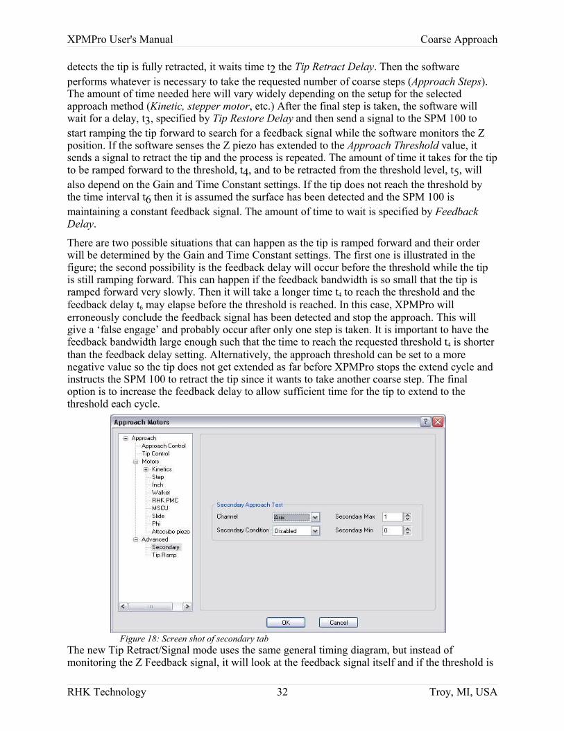
Advanced approach settings
The secondary tab (as shown in Figure 18) contains the settings that allow a second channel to be monitored during approach. For some systems there are two signals that may change and if either one shifts dramatically the approach should stop. An example is non-contact AFM where the frequency can shift out of resonance spontaneously and the amplitude can decrease. Since the feedback loop can only monitor one of these, this feature provides a second level of tip protection. A second signal can be sent to an Aux channel and be checked after each step. A ‘safe’ range can be designated and if the signal goes outside these boundaries, the approach will
be stopped and manual adjustments made (sweep frequency again, etc.) to return the monitored signal to its normal condition. Select the signal to be monitored using the Channel entry box. The output of the signal should be connected to this rear panel BNC on the SPM 100. Choose the type of Secondary condition to test. Valid selections are Safe between limits, safe outside limits, safe below maximum and safe above minimum or Disabled to have the approach only depend on the primary channel (topography for tip retract and feedback detect, feedback signal for all others). Secondary Max is the upper boundary of the secondary signal Secondary Min is the lower boundary of the secondary signal.
RHK Technology 33 Troy, MI, USA
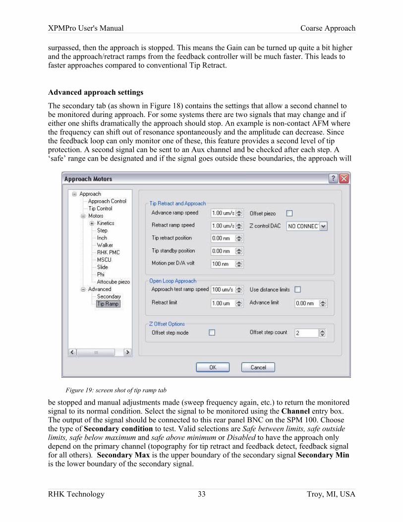
Figure 19: screen shot of tip ramp tab
XPMPro User's Manual Coarse Approach
The tab that controls the open loop ramp and the z offset step mode is shown in Figure 22. Most users will not have to set any parameters in this tab unless Open Loop Ramp is in use as the approach mode or Analog Ramp has been selected for tip control instead of the TTL Feedback default.
The first set of parameters are used to configure the analog ramp when TTL Feedback has not been chosen as tip control mode. The Advance ramp speed sets the speed that the tip is moved towards the surface. The speed should be slow enough to ensure the change in feedback signal is detected before the tip moves far enough to create unwanted contact. This speed is usually determined by the bandwidth of the detector circuit. The Retract ramp speed sets the speed that the tip is retracted if no response was detected during the tip ramp. It can be set to a higher value than approach since no monitoring is necessary and a faster approach cycle can be achieved. The Tip retract distance determines how far to pull the tip back. If mechanical constraints require the tip not get pulled back its maximum retraction, use this value to limit how far the tip moves from its fully retracted position. Motion per D/A volt will depend on the vertical calibration of the Z piezo and the BNC the DAC ramp is applied to. This value must be known relatively accurately or tip crashes can occur.
If using the Open loop ramp approach mode to improve the speed of tip-sample approach, then the second group of parameters are used to determine settings specific to this mode. The Approach test ramp speed is the rate to advance the tip after each coarse step. This can be quite high since the feedback signal will be detected very quickly with the loop open. The maximum speed will depend on the total distance that can be traveled between the height where a signal can be detected and a tip crash. The current depends exponentially on the distance above the surface in STM so a reasonable value may be 1 nm. If the tip is more than 1 nm above the surface, the current will be zero. If the height reaches zero, the tip is crashed. Therefore, the speed cannot be greater than traveling this 1 nm distance in less than the 20 ms response of a typical current to voltage circuit. This means the speed should be less than 1 nm/20 ms which is ~50 mm/s. For NSOM or AFM where the interactions are longer ranged (maybe 2 nm), but the signal circuit is also usually slower (time constant of a lock-in amplifier of 3 ms), a ramp speed of 0.33 mm/s is possible. To avoid ramping the z piezo over its full range turn ON Use distance limits. This may be useful if there are resonances present in the scan head design which are excited when the Z piezo is near full extension or full retraction. Also if the z piezo is modulated to excite a cantilever, when the piezo is fully extended or contracted the excitation will not be correct since the motion gets clipped at its endpoints. In this case, the range can be centered about zero volts or the piezo element's equilibrium length. Min and Max limits are used to restrict the range of motion. The Z calibration of the piezo element must be reasonably accurate or the actual distance will differ from the entered values. The z=0 distance is the value when the z piezo is at its equilibrium length.
There are some scan
RHK Technology 34 Troy, MI, USA
Figure 20:Timing diagram with Z Offset Step Mode and Tip Retract
XPMPro User's Manual Coarse Approach
heads in existence where the coarse step size cannot be made smaller than the z piezo range. In these models, it is necessary to add a separate piezo element for z offset which must be extended stepwise between each coarse step to “fill in” the motion taken by large coarse steps. The piezo starts out fully contracted and if no feedback signal is detected instead of taking another coarse step, the offset piezo is extended a fixed amount and the feedback signal checked again. This is repeated until the offset piezo is fully extended and if there is still no signal, then a coarse step is taken. A timing diagram if Z Offset Step Mode used with Tip Retract is shown in Figure 20. A coarse step is taken after both piezo's are retracted and then the next coarse step is not taken until the end of the diagram when both signals are again in the fully retracted position. Since the offset piezo overlaps the range of the coarse step, it is safe to step forward again and be assured the z scan element will not be fully saturated in the contracted position. Offset step mode should be ON to utilize this offset stepwise mode and Z offset piezo should be checked when the DAC is controlling a separate z piezo element instead the one controlled by the analog feedback loop. However, be sure to fully understand how the head performs and what the advantages are before turning this on as a tip crash can occur if the software is misconfigured. The Z Control DAC selects which output DAC on the rear panel of the SPM 100 is connected to the input that controls the offset piezo. In most cases this is the Z Offset External Control. The voltage ramp to move the piezo is applied to this channel.
It is strongly recommended to use this mode when operating the Unisoku low temperature microscopes. The z piezo range is quite limited in these microscopes in order to achieve high z sensitivity and the step size usually covered by the coarse motor is larger than this z range.
Configuring approach motors
XPMPro can operate an incredibly diverse set of motors typically used on SPM heads. Some of them require an additional TTL card (DT335) to produce pulses and some of them use the TTL line included on the DT3016 board. The use of the PMC100 from RHK will require an additional network connection for communication between XPMPro and the unit. Other approach methods use one or two of the rear panel DACs to produce waveforms that will be amplified by the high voltage amplifiers and applied to a piezo element.
Kinetic approach systems
Kinetic approach systems, also called inertial or slip-stick approach systems, utilize a sawtooth-shaped (or other shaped) waveform to drive a piezo tube, shear-mode piezo stack, or walker-type SPM's. By slowly expanding and then quickly contracting their length, they can produce translations along the axes. Two parameter windows are used to define the necessary functions for kinetic approach heads. After selecting the Kinetic Waveform option for approach mode, select the Wave1 tab (as shown as Figure 21) and then enter the parameters appropriate for the scan head in use.
If the Dual kinetic waveform is selected then the same set of parameters can be specified in the Wave2 tab. Additionally an extra parameter in the Wave2 tab (as shown as Figure 22) allows the user to specify if the Wave2 polarity should also be reversed when Tip Retract is chosen. These two signals will be output on different DAC channels and can be then be summed into different piezo segments depending on what BNC the DAC output is applied to. All of the settings for Wave1 are present for Wave2 along with the additional parameter to introduce a phase shift between the two signals (Offset from primary).
XPMPro allows five different waveforms to be used for different scan head systems. Choose the correct shape for the head in use in the Waveform entry. A UHV300 STM or UHV350 AFM
RHK Technology 35 Troy, MI, USA
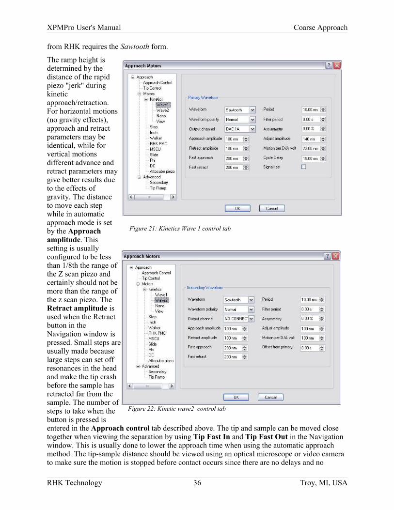
XPMPro User's Manual Coarse Approach
from RHK requires the Sawtooth form.
The ramp height is determined by the distance of the rapid piezo "jerk" during kinetic approach/retraction. For horizontal motions (no gravity effects), approach and retract parameters may be identical, while for vertical motions different advance and retract parameters may give better results due to the effects of gravity. The distance to move each step while in automatic approach mode is set by the Approach amplitude. This setting is usually configured to be less than 1/8th the range of the Z scan piezo and certainly should not be more than the range of the z scan piezo. The Retract amplitude is used when the Retract button in the Navigation window is pressed. Small steps are usually made because large steps can set off resonances in the head and make the tip crash before the sample has retracted far from the sample. The number of steps to take when the button is pressed is entered in the Approach control tab described above. The tip and sample can be moved close together when viewing the separation by using Tip Fast In and Tip Fast Out in the Navigation window. This is usually done to lower the approach time when using the automatic approach method. The tip-sample distance should be viewed using an optical microscope or video camera to make sure the motion is stopped before contact occurs since there are no delays and no
RHK Technology 36 Troy, MI, USA
Figure 21: Kinetics Wave 1 control tab
Figure 22: Kinetic wave2 control tab
XPMPro User's Manual Coarse Approach
checking of threshold levels. The amount of travel in each step when fast motion takes place is entered in the Fast Approach and Fast retract step size box. For horizontal motions (no effects of gravity), approach and retract parameters may be identical, while for vertical motions different advance and retract parameters may give better results. To take a single step in a direction, the '+' and '-' buttons on the Navigation window should be clicked. The Adjust amplitude sets the distance moved each time a button is pressed. This is normally used when the scan head is already within imaging range of the surface but the user wants to make small steps to better center the z piezo extension about its equilibrium position or to move the tip/sample laterally to image a different part of the surface. The distance is normally small, typically no more than 5-10% of the Z scan range. All of these motions are calibrated with respect to the Motion per D/A volt setting. The low voltage ramp before the high voltage amplifiers is always the ratio between the amplitude entered above and this value. If the Adjust amplitude is 100 nm and the Motion per D/A volt is 20 nm a 5 V signal is produced just like if the Adjust amplitude is 500 nm and the Motion per D/A volt is 100 nm. The sign is significant so if a tip approach actually moves the tip and sample further apart, set this parameter to a negative number if it was originally positive.
The amount of time it should take to complete one waveform cycle is set by the Period. The waveform output can be high pass filtered in order to reduce the sharpness of some edges. This can be necessary for certain microscope head designs that have high resonance frequencies. The high frequency components of the waveforms can be filtered out to avoid unnecessary shaking of the head that can lead to tip crashes and other undesirable results when approaching. This filtering capability can provide the same functionality as the Inertial Filter knob on the front panel of the SPM 100. The width of the filter is determined by the Filter Period. A value of zero seconds means no filtering is applied and the waveform will be generated at the maximum possible rate of 250 kHz when using the DT3016 board. Use the Asymmetry setting to determine the variation from an ideal sawtooth waveform. A value of 0 means the shape is a perfect sawtooth with an instantaneous drop to 0, while a setting of 10% means 10% of the period is taken on the falling edge and 90% is on the rising section. The Cycle delay is used when fast motion is taking place. With no feedback checking between steps, the ramps can be as close together as requested. Use Cycle delay to allow some time to elapse between each coarse step in order for transients introduced in the head by the jerking motion to decay.
The D/A output channel on the rear panel used to drive the coarse approach is chosen using the Output channel setting. A BNC-BNC JUMPER MUST BE ATTACHED BETWEEN THIS OUTPUT CHANNEL AND THE APPROPRIATE INPUT ON THE REAR PANEL OF THE SPM 100.
The ramp is usually produced from 0 up to 10 volts. Since the DAC can actually range from -10 V to +10 V, larger steps are possible if needed. When Waveform polarity is set to Normal the ramp will always be positive. If the step size requested is larger than can be produced by ramping from 0 V to +10 V, then the user has the choice of ramping around zero symmetrically (symmetric bipolar) or to use the full positive value and use as large of a negative voltage needed to reach the requested step size. If the ratio between Approach amplitude and Motion per D/A volt is 16, the DAC will ramp from -8 V to +8 V is this is set to symmetric bipolar or it will ramp from -6 V to +10 V if bipolar allowed is chosen.
FAQ: Tip approach and retract is not working?
Solution Step:
1. make sure that scan head manipulator does not touch the scan head
RHK Technology 37 Troy, MI, USA
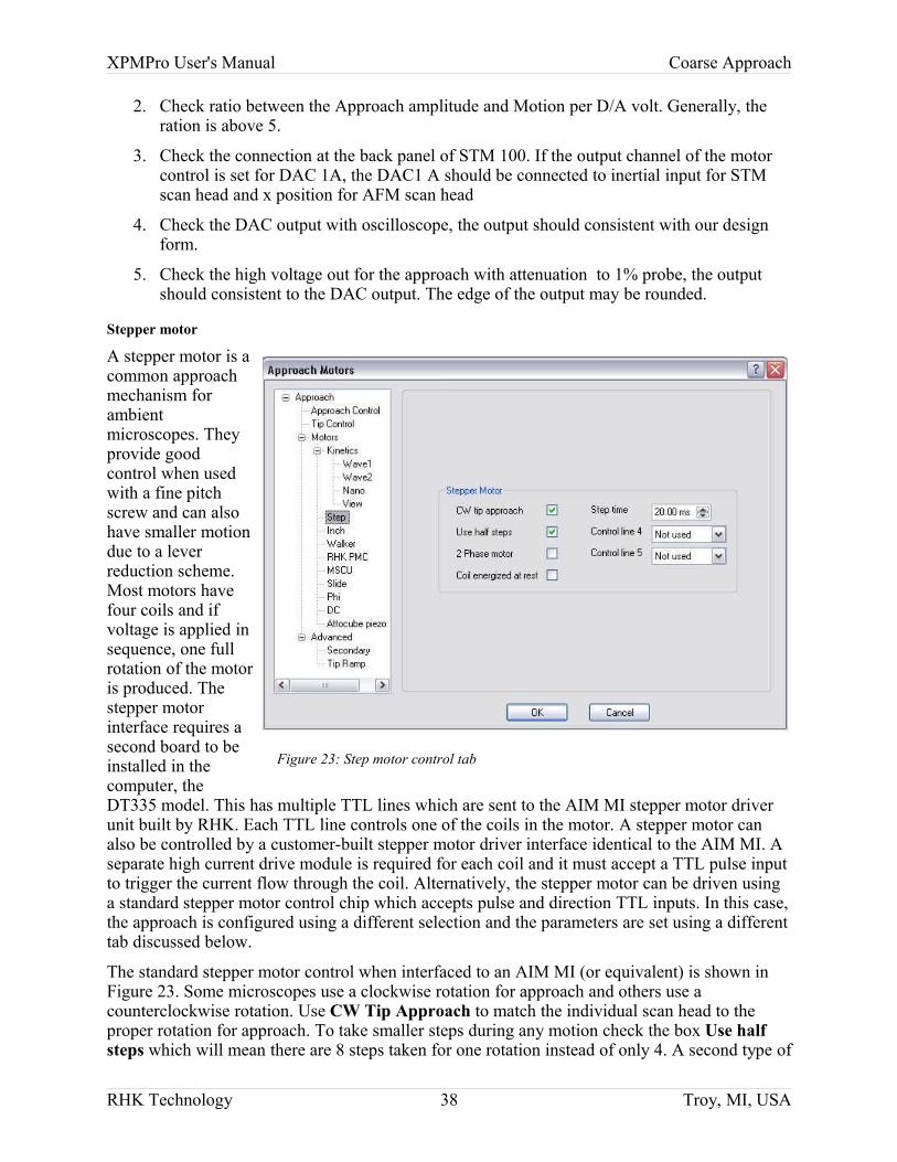
XPMPro User's Manual Coarse Approach
2. Check ratio between the Approach amplitude and Motion per D/A volt. Generally, the ration is above 5.
3. Check the connection at the back panel of STM 100. If the output channel of the motor control is set for DAC 1A, the DAC1 A should be connected to inertial input for STM scan head and x position for AFM scan head
4. Check the DAC output with oscilloscope, the output should consistent with our design form.
5. Check the high voltage out for the approach with attenuation to 1% probe, the output should consistent to the DAC output. The edge of the output may be rounded.
Stepper motor
A stepper motor is a common approach mechanism for ambient microscopes. They provide good control when used with a fine pitch screw and can also have smaller motion due to a lever reduction scheme. Most motors have four coils and if voltage is applied in sequence, one full rotation of the motor is produced. The stepper motor interface requires a second board to be installed in the computer, the DT335 model. This has multiple TTL lines which are sent to the AIM MI stepper motor driver unit built by RHK. Each TTL line controls one of the coils in the motor. A stepper motor can also be controlled by a customer-built stepper motor driver interface identical to the AIM MI. A separate high current drive module is required for each coil and it must accept a TTL pulse input to trigger the current flow through the coil. Alternatively, the stepper motor can be driven using a standard stepper motor control chip which accepts pulse and direction TTL inputs. In this case, the approach is configured using a different selection and the parameters are set using a different tab discussed below.
The standard stepper motor control when interfaced to an AIM MI (or equivalent) is shown in Figure 23. Some microscopes use a clockwise rotation for approach and others use a counterclockwise rotation. Use CW Tip Approach to match the individual scan head to the proper rotation for approach. To take smaller steps during any motion check the box Use half steps which will mean there are 8 steps taken for one rotation instead of only 4. A second type of
RHK Technology 38 Troy, MI, USA
Figure 23: Step motor control tab
XPMPro User's Manual Coarse Approach
stepper motor is considered 2 phase because it requires two coils to be energized simultaneously for the motor to turn properly. This motor is used in conjunction with an AIM NSOM from RHK when connected to a Nanonics NSOM head and an AIM DI when operating a Bioscope. In this case make sure 2 phase motor is checked.
Most stepper motors require a large current to produce rotation. When no motion is taking place the voltages to each coil should be set to zero so no current flow is occurring. The current will dramatically heat up the motor and subsequently the entire scan head which will cause significant thermal drift problems. However, some scan head designs will require the coil to be energized in order to resist motion of the motor due to gravity. If the motor holds precise position without voltage on the coils, Coil energized at rest can remain unchecked. The pulse width of the TTL signals will determine the speed of motion. However, do not set the pulse width too short or no motion can occur because the coil will not be energized long enough to turn the shaft. Change the Step time setting until the approach velocity is adequate. For most motors a few milliseconds is sufficiently long to produce rotation. When using an AIM NSOM, there are separate lines required to remove the current flow from the two phase motor in use. In this case adjust the Control line 4 and Control line 5 settings until motion occurs. If an AIM MI is in use, these can be left at Not used.
Omicron 8 channel MSCU
The eight channel MSCU features 8 output channels that can be controlled via a handset, the serial connection, or using the rear panel SYNC connection. The recommended method is to use the serial connection between an RS232 port on the host PC and the MSCU.
The configuration window is shown in Figure 24. The MSCU Control Mode can be set set to TTL control, serial interface, or analog DAC control. If using the TTL option, a BNC cable should connect TTL OUT on the DT3016 adapter box to the rear panel SYNC connector. If using a version 8.5 SPM100, the TTL output is located on pin 15 of the rear panel Digital IO connector. Use the handset to place the MSCU in external mode so the steps are synchronized with the SPM100 feedback test. Refer to the MSCU manual for the steps of placing the +Z channel to be controlled by the SYNC connection. When the approach is initiated, a message will appear to remind the user to place the MSCU external mode in +Z channel. After the approach is finished, the handset can be used to return the MSCU to internal mode to avoid accidental motion of the motor or can be left in external in case additional forward steps under computer control are desired. If backwards steps are requested, the window will appear asking to change the MSCU external mode to the -Z channel so each TTL pulse produces reverse motion.
The preferred method is to use the serial connection. This allows any channel to be controlled and the parameters of the motion (step time, voltage level, etc.) can all be changed via commands. When this option is chosen enter the serial port the MSCU is connected to in COM port entry box. The channel to be used when a coarse approach should move the tip and sample close together is chosen using the Approach channel setting. In most cases this will be channel 3 which is the first z channel. Refer to the MSCU manual to find out which channel is connected to the z coarse motor. If the approach moves in the wrong direction change the setting of the Invert approach motion check box. To move any of the 8 motors interactively click on Open XYZ Control in the main NAV window to open the control window which contains a set of buttons for all motor channels. The number of steps moved each time one of the buttons is clicked is set using the Steps per click parameter. To have XPMPro initialize the MSCU when the program starts, check the MSCU connected box so serial communication is established when XPMPro starts.
RHK Technology 39 Troy, MI, USA
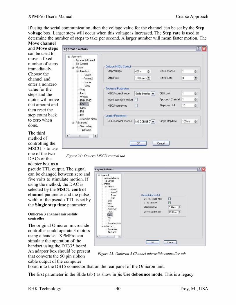
XPMPro User's Manual Coarse Approach
If using the serial communication, then the voltage value for the channel can be set by the Step voltage box. Larger steps will occur when this voltage is increased. The Step rate is used to determine the number of steps to take per second. A larger number will mean faster motion. The Move channel and Move steps can be used to move a fixed number of steps immediately. Choose the channel and enter a nonzero value for the steps and the motor will move that amount and then reset the step count back to zero when done.
The third method of controlling the MSCU is to use one of the two DACs of the adapter box as a pseudo TTL output. The signal can be changed between zero and five volts to stimulate motion. If using the method, the DAC is selected by the MSCU control channel parameter and the pulse width of the pseudo TTL is set by the Single step time parameter.
Omicron 3 channel microslide controller
The original Omicron microslide controller could operate 3 motors using a handset. XPMPro can simulate the operation of the handset using the DT335 board. An adapter box should be present that converts the 50 pin ribbon cable output of the computer board into the DB15 connector that on the rear panel of the Omicron unit.
The first parameter in the Slide tab ( as show in )is Use debounce mode. This is a legacy
RHK Technology 40 Troy, MI, USA
Figure 24: Omicro MSCU control tab
Figure 25: Omicron 3 Channel microslide controller tab
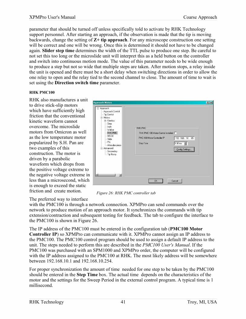
XPMPro User's Manual Coarse Approach
parameter that should be turned off unless specifically told to activate by RHK Technology support personnel. After starting an approach, if the observation is made that the tip is moving backwards, change the setting of Z+ tip approach. For any microscope construction one setting will be correct and one will be wrong. Once this is determined it should not have to be changed again. Slider step time determines the width of the TTL pulse to produce one step. Be careful to not set this too long or the microslide unit will interpret this as a held button on the controller and switch into continuous motion mode. The value of this parameter needs to be wide enough to produce a step but not so wide that multiple steps are taken. After motion stops, a relay inside the unit is opened and there must be a short delay when switching directions in order to allow the one relay to open and the relay tied to the second channel to close. The amount of time to wait is set using the Direction switch time parameter.
RHK PMC100
RHK also manufactures a unit to drive stick-slip motors which have sufficiently high friction that the conventional kinetic waveform cannot overcome. The microslide motors from Omicron as well as the low temperature motor popularized by S.H. Pan are two examples of this construction. The motor is driven by a parabolic waveform which drops from the positive voltage extreme to the negative voltage extreme in less than a microsecond, which is enough to exceed the static friction and create motion.
The preferred way to interface with the PMC100 is through a network connection. XPMPro can send commands over the network to produce motion of an approach motor. It synchronizes the commands with tip extension/contraction and subsequent testing for feedback. The tab to configure the interface to the PMC100 is shown in Figure 26.
The IP address of the PMC100 must be entered in the configuration tab (PMC100 Motor Controller IP) so XPMPro can communicate with it. XPMPro cannot assign an IP address to the PMC100. The PMC100 control program should be used to assign a default IP address to the unit. The steps needed to perform this are described in the PMC100 User's Manual. If the PMC100 was purchased with an SPM1000 and XPMPro order, the computer will be configured with the IP address assigned to the PMC100 at RHK. The most likely address will be somewhere between 192.168.10.1 and 192.168.10.254.
For proper synchronization the amount of time needed for one step to be taken by the PMC100 should be entered in the Step Time box. The actual time depends on the characteristics of the motor and the settings for the Sweep Period in the external control program. A typical time is 1 millisecond.
RHK Technology 41 Troy, MI, USA
Figure 26: RHK PMC controller tab
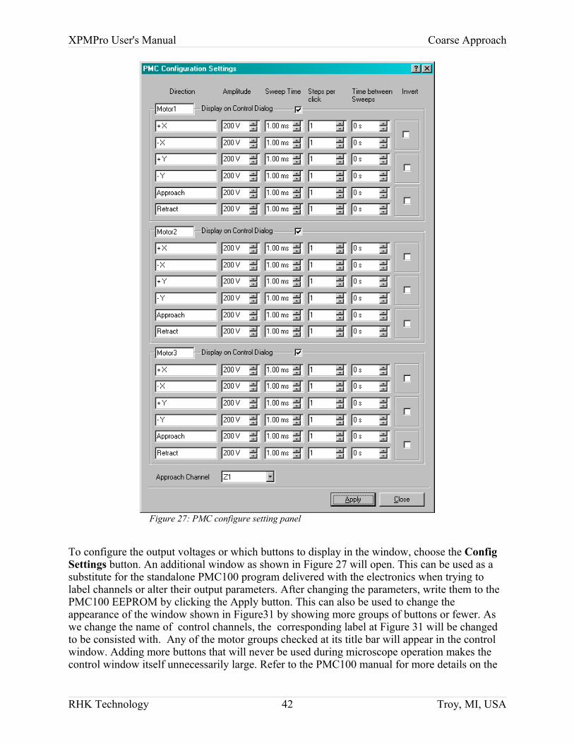
XPMPro User's Manual Coarse Approach
To configure the output voltages or which buttons to display in the window, choose the Config Settings button. An additional window as shown in Figure 27 will open. This can be used as a substitute for the standalone PMC100 program delivered with the electronics when trying to label channels or alter their output parameters. After changing the parameters, write them to the PMC100 EEPROM by clicking the Apply button. This can also be used to change the appearance of the window shown in Figure31 by showing more groups of buttons or fewer. As we change the name of control channels, the corresponding label at Figure 31 will be changed to be consisted with. Any of the motor groups checked at its title bar will appear in the control window. Adding more buttons that will never be used during microscope operation makes the control window itself unnecessarily large. Refer to the PMC100 manual for more details on the
RHK Technology 42 Troy, MI, USA
Figure 27: PMC configure setting panel
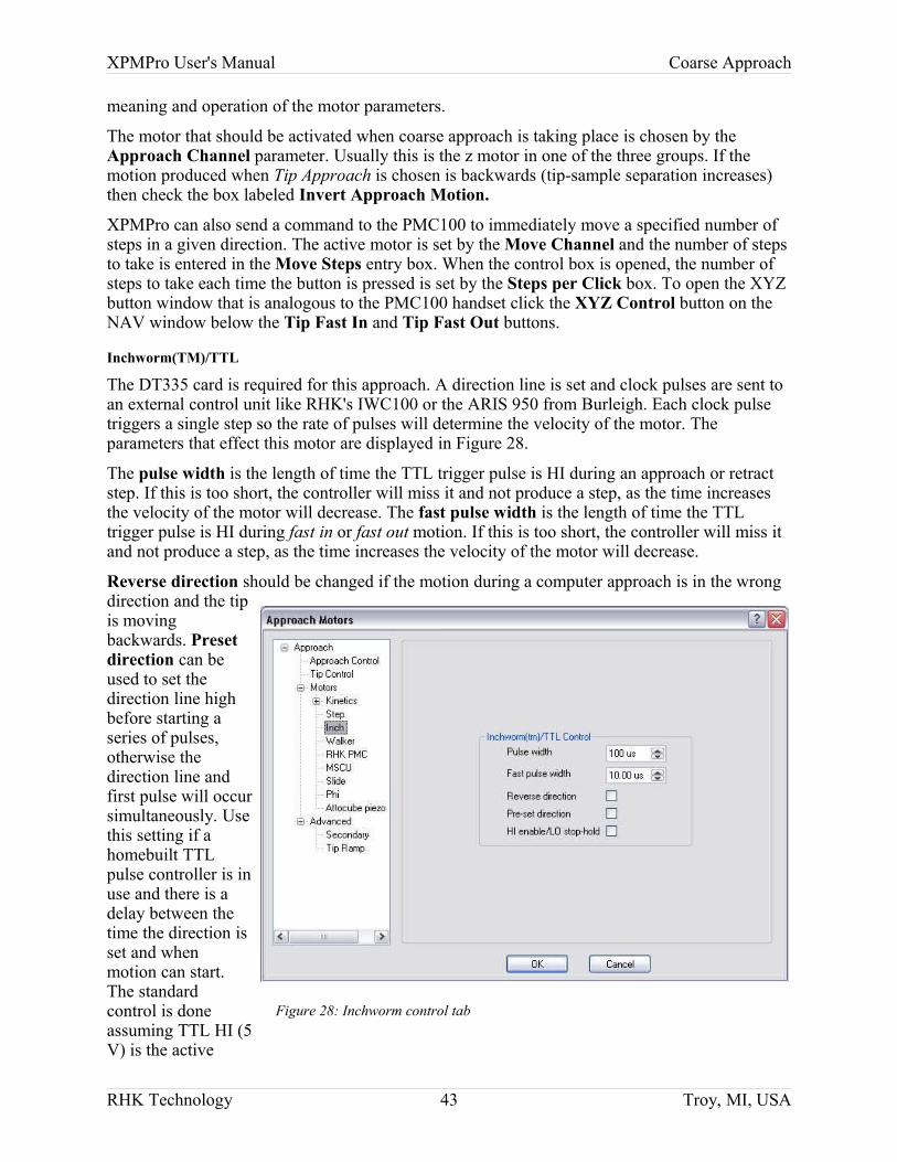
XPMPro User's Manual Coarse Approach
meaning and operation of the motor parameters.
The motor that should be activated when coarse approach is taking place is chosen by the Approach Channel parameter. Usually this is the z motor in one of the three groups. If the motion produced when Tip Approach is chosen is backwards (tip-sample separation increases) then check the box labeled Invert Approach Motion.
XPMPro can also send a command to the PMC100 to immediately move a specified number of steps in a given direction. The active motor is set by the Move Channel and the number of steps to take is entered in the Move Steps entry box. When the control box is opened, the number of steps to take each time the button is pressed is set by the Steps per Click box. To open the XYZ button window that is analogous to the PMC100 handset click the XYZ Control button on the NAV window below the Tip Fast In and Tip Fast Out buttons.
Inchworm(TM)/TTL
The DT335 card is required for this approach. A direction line is set and clock pulses are sent to an external control unit like RHK's IWC100 or the ARIS 950 from Burleigh. Each clock pulse triggers a single step so the rate of pulses will determine the velocity of the motor. The parameters that effect this motor are displayed in Figure 28.
The pulse width is the length of time the TTL trigger pulse is HI during an approach or retract step. If this is too short, the controller will miss it and not produce a step, as the time increases the velocity of the motor will decrease. The fast pulse width is the length of time the TTL trigger pulse is HI during fast in or fast out motion. If this is too short, the controller will miss it and not produce a step, as the time increases the velocity of the motor will decrease.
Reverse direction should be changed if the motion during a computer approach is in the wrong direction and the tip is moving backwards. Preset direction can be used to set the direction line high before starting a series of pulses, otherwise the direction line and first pulse will occur simultaneously. Use this setting if a homebuilt TTL pulse controller is in use and there is a delay between the time the direction is set and when motion can start. The standard control is done assuming TTL HI (5 V) is the active
RHK Technology 43 Troy, MI, USA
Figure 28: Inchworm control tab
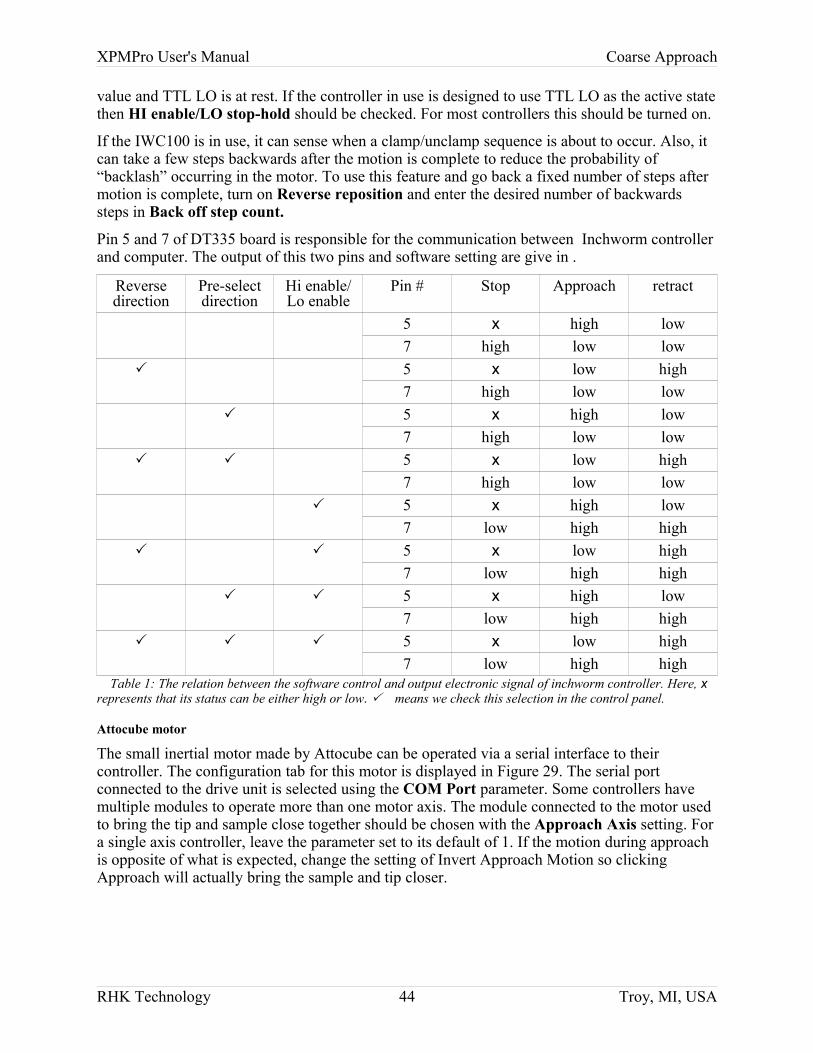
XPMPro User's Manual Coarse Approach
value and TTL LO is at rest. If the controller in use is designed to use TTL LO as the active state then HI enable/LO stop-hold should be checked. For most controllers this should be turned on.
If the IWC100 is in use, it can sense when a clamp/unclamp sequence is about to occur. Also, it can take a few steps backwards after the motion is complete to reduce the probability of “backlash” occurring in the motor. To use this feature and go back a fixed number of steps after motion is complete, turn on Reverse reposition and enter the desired number of backwards steps in Back off step count.
Pin 5 and 7 of DT335 board is responsible for the communication between Inchworm controller and computer. The output of this two pins and software setting are give in .
Reverse direction
Pre-select direction
Hi enable/ Lo enable
Pin # Stop Approach retract
5 x high low7 high low low
5 x low high7 high low low
5 x high low7 high low low
5 x low high7 high low low
5 x high low7 low high high
5 x low high7 low high high
5 x high low7 low high high
5 x low high7 low high high
Table 1: The relation between the software control and output electronic signal of inchworm controller. Here, x represents that its status can be either high or low. means we check this selection in the control panel.
Attocube motor
The small inertial motor made by Attocube can be operated via a serial interface to their controller. The configuration tab for this motor is displayed in Figure 29. The serial port connected to the drive unit is selected using the COM Port parameter. Some controllers have multiple modules to operate more than one motor axis. The module connected to the motor used to bring the tip and sample close together should be chosen with the Approach Axis setting. For a single axis controller, leave the parameter set to its default of 1. If the motion during approach is opposite of what is expected, change the setting of Invert Approach Motion so clicking Approach will actually bring the sample and tip closer.
RHK Technology 44 Troy, MI, USA
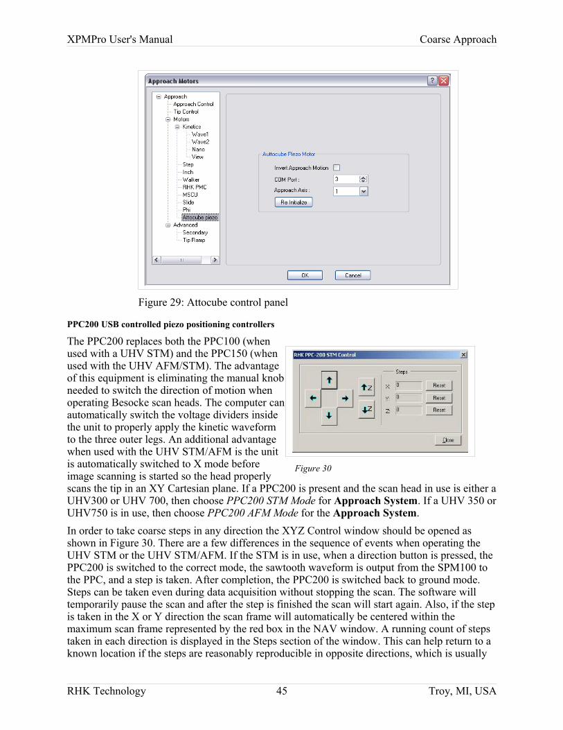
XPMPro User's Manual Coarse Approach
PPC200 USB controlled piezo positioning controllers
The PPC200 replaces both the PPC100 (when used with a UHV STM) and the PPC150 (when used with the UHV AFM/STM). The advantage of this equipment is eliminating the manual knob needed to switch the direction of motion when operating Besocke scan heads. The computer can automatically switch the voltage dividers inside the unit to properly apply the kinetic waveform to the three outer legs. An additional advantage when used with the UHV STM/AFM is the unit is automatically switched to X mode before image scanning is started so the head properly scans the tip in an XY Cartesian plane. If a PPC200 is present and the scan head in use is either a UHV300 or UHV 700, then choose PPC200 STM Mode for Approach System. If a UHV 350 or UHV750 is in use, then choose PPC200 AFM Mode for the Approach System. In order to take coarse steps in any direction the XYZ Control window should be opened as shown in Figure 30. There are a few differences in the sequence of events when operating the UHV STM or the UHV STM/AFM. If the STM is in use, when a direction button is pressed, the PPC200 is switched to the correct mode, the sawtooth waveform is output from the SPM100 to the PPC, and a step is taken. After completion, the PPC200 is switched back to ground mode. Steps can be taken even during data acquisition without stopping the scan. The software will temporarily pause the scan and after the step is finished the scan will start again. Also, if the step is taken in the X or Y direction the scan frame will automatically be centered within the maximum scan frame represented by the red box in the NAV window. A running count of steps taken in each direction is displayed in the Steps section of the window. This can help return to a known location if the steps are reasonably reproducible in opposite directions, which is usually
RHK Technology 45 Troy, MI, USA
Figure 29: Attocube control panel
Figure 30
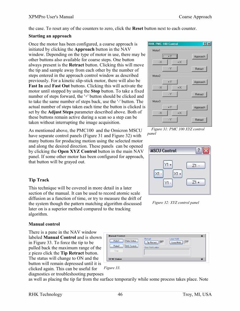
XPMPro User's Manual Coarse Approach
the case. To reset any of the counters to zero, click the Reset button next to each counter.Starting an approach
Once the motor has been configured, a coarse approach is initiated by clicking the Approach button in the NAV window. Depending on the type of motor in use, there may be other buttons also available for coarse steps. One button always present is the Retract button. Clicking this will move the tip and sample away from each other by the number of steps entered in the approach control window as described previously. For a kinetic slip-stick motor, there will also be Fast In and Fast Out buttons. Clicking this will activate the motor until stopped by using the Stop button. To take a fixed number of steps forward, the '+' button should be clicked and to take the same number of steps back, use the '-' button. The actual number of steps taken each time the button is clicked is set by the Adjust Steps parameter described above. Both of these buttons remain active during a scan so a step can be taken without interrupting the image acquisition.
As mentioned above, the PMC100 and the Omicron MSCU have separate control panels (Figure 31 and Figure 32) with many buttons for producing motion using the selected motor and along the desired direction. These panels can be opened by clicking the Open XYZ Control button in the main NAV panel. If some other motor has been configured for approach, that button will be grayed out.
Tip Track
This technique will be covered in more detail in a later section of the manual. It can be used to record atomic scale diffusion as a function of time, or try to measure the drift of the system though the pattern matching algorithm discussed later on is a superior method compared to the tracking algorithm.
Manual control
There is a pane in the NAV window labeled Manual Control and is shown in Figure 33. To force the tip to be pulled back the maximum range of the z piezo click the Tip Retract button. The status will change to ON and the button will remain depressed until it is clicked again. This can be useful for diagnostics or troubleshooting purposes as well as placing the tip far from the surface temporarily while some process takes place. Note
RHK Technology 46 Troy, MI, USA
Figure 33.
Figure 32: XYZ control panel
Figure 31: PMC 100 XYZ control panel
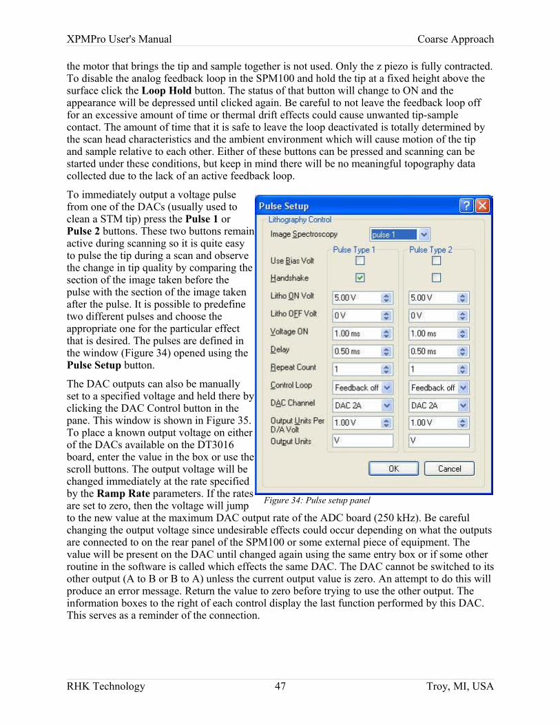
XPMPro User's Manual Coarse Approach
the motor that brings the tip and sample together is not used. Only the z piezo is fully contracted. To disable the analog feedback loop in the SPM100 and hold the tip at a fixed height above the surface click the Loop Hold button. The status of that button will change to ON and the appearance will be depressed until clicked again. Be careful to not leave the feedback loop off for an excessive amount of time or thermal drift effects could cause unwanted tip-sample contact. The amount of time that it is safe to leave the loop deactivated is totally determined by the scan head characteristics and the ambient environment which will cause motion of the tip and sample relative to each other. Either of these buttons can be pressed and scanning can be started under these conditions, but keep in mind there will be no meaningful topography data collected due to the lack of an active feedback loop.
To immediately output a voltage pulse from one of the DACs (usually used to clean a STM tip) press the Pulse 1 or Pulse 2 buttons. These two buttons remain active during scanning so it is quite easy to pulse the tip during a scan and observe the change in tip quality by comparing the section of the image taken before the pulse with the section of the image taken after the pulse. It is possible to predefine two different pulses and choose the appropriate one for the particular effect that is desired. The pulses are defined in the window (Figure 34) opened using the Pulse Setup button.
The DAC outputs can also be manually set to a specified voltage and held there by clicking the DAC Control button in the pane. This window is shown in Figure 35. To place a known output voltage on either of the DACs available on the DT3016 board, enter the value in the box or use the scroll buttons. The output voltage will be changed immediately at the rate specified by the Ramp Rate parameters. If the rates are set to zero, then the voltage will jump to the new value at the maximum DAC output rate of the ADC board (250 kHz). Be careful changing the output voltage since undesirable effects could occur depending on what the outputs are connected to on the rear panel of the SPM100 or some external piece of equipment. The value will be present on the DAC until changed again using the same entry box or if some other routine in the software is called which effects the same DAC. The DAC cannot be switched to its other output (A to B or B to A) unless the current output value is zero. An attempt to do this will produce an error message. Return the value to zero before trying to use the other output. The information boxes to the right of each control display the last function performed by this DAC. This serves as a reminder of the connection.
RHK Technology 47 Troy, MI, USA
Figure 34: Pulse setup panel
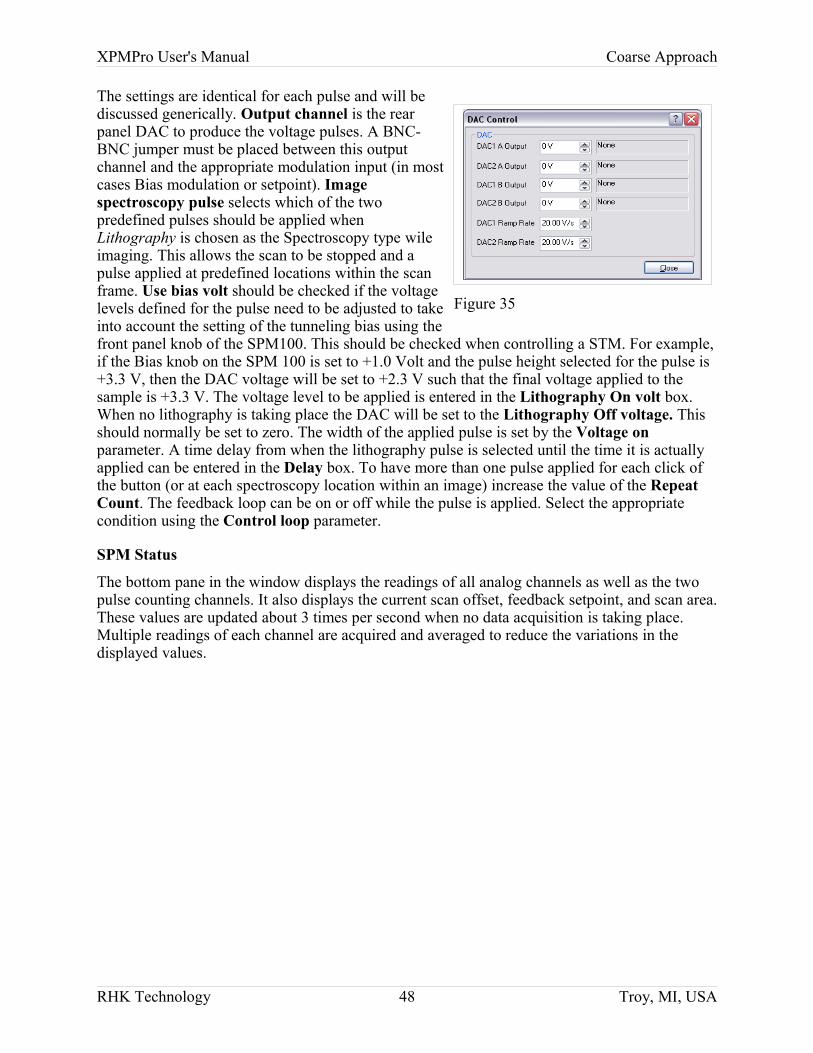
XPMPro User's Manual Coarse Approach
The settings are identical for each pulse and will be discussed generically. Output channel is the rear panel DAC to produce the voltage pulses. A BNC-BNC jumper must be placed between this output channel and the appropriate modulation input (in most cases Bias modulation or setpoint). Image spectroscopy pulse selects which of the two predefined pulses should be applied when Lithography is chosen as the Spectroscopy type wile imaging. This allows the scan to be stopped and a pulse applied at predefined locations within the scan frame. Use bias volt should be checked if the voltage levels defined for the pulse need to be adjusted to take into account the setting of the tunneling bias using the front panel knob of the SPM100. This should be checked when controlling a STM. For example, if the Bias knob on the SPM 100 is set to +1.0 Volt and the pulse height selected for the pulse is +3.3 V, then the DAC voltage will be set to +2.3 V such that the final voltage applied to the sample is +3.3 V. The voltage level to be applied is entered in the Lithography On volt box. When no lithography is taking place the DAC will be set to the Lithography Off voltage. This should normally be set to zero. The width of the applied pulse is set by the Voltage on parameter. A time delay from when the lithography pulse is selected until the time it is actually applied can be entered in the Delay box. To have more than one pulse applied for each click of the button (or at each spectroscopy location within an image) increase the value of the Repeat Count. The feedback loop can be on or off while the pulse is applied. Select the appropriate condition using the Control loop parameter.
SPM Status
The bottom pane in the window displays the readings of all analog channels as well as the two pulse counting channels. It also displays the current scan offset, feedback setpoint, and scan area. These values are updated about 3 times per second when no data acquisition is taking place. Multiple readings of each channel are acquired and averaged to reduce the variations in the displayed values.
RHK Technology 48 Troy, MI, USA
Figure 35

XPMPro User's Manual Initial Acquisition
Initial Acquisition
RHK Technology 49 Troy, MI, USA
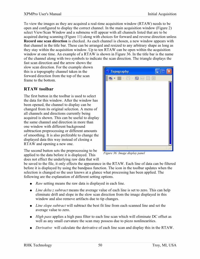
XPMPro User's Manual Initial Acquisition
To view the images as they are acquired a real-time acquisition window (RTAW) needs to be open and configured to display the correct channel. In the main acquisition window (Figure 2) select View/Scan Window and a submenu will appear with all channels listed that are to be acquired during scanning (Figure 11) along with choices for forward and reverse direction unless Record one scan direction is checked. As each channel is chosen, a new window appears with that channel in the title bar. These can be arranged and resized to any arbitrary shape as long as they stay within the acquisition window. Up to ten RTAW can be open within the acquisition window at one time. An example of a RTAW is shown in Figure 36. In the title bar is the name of the channel along with two symbols to indicate the scan direction. The triangle displays the fast scan direction and the arrow shows the slow scan direction. For the example shown this is a topography channel taken in the forward direction from the top of the scan frame to the bottom.
RTAW toolbarThe first button in the toolbar is used to select the data for this window. After the window has been opened, the channel to display can be changed from its original selection. A menu of all channels and directions currently being acquired is shown. This can be useful to display the same channel and direction in more than one window with different background subtraction preprocessing or different amounts of smoothing. It is also preferable to change the displayed data this way instead of closing a RTAW and opening a new one.
The second button sets the preprocessing to be applied to the data before it is displayed. This does not effect the underlying raw data that will be saved to the file, it only effects the appearance in the RTAW. Each line of data can be filtered before it is displayed by using the bandpass function. The icon in the toolbar updates when the selection is changed so the user knows at a glance what processing has been applied. The following are the explanation of different setting options.
● Raw setting means the raw data is displayed in each line.
● Line delta z subtract means the average value of each line is set to zero. This can help eliminate drift and slope in the slow scan direction from the image displayed in this window and also remove artifacts due to tip changes.
● Line slope subtract will subtract the best fit line from each scanned line and set the average value to zero.
● High pass applies a high pass filter to each line scan which will eliminate DC offset as well as any small curvature the scan may possess due to piezo nonlinearities.
● Derivative will calculate the derivative of each line scan and display this in the RTAW.
RHK Technology 50 Troy, MI, USA
Figure 36: Image display panel
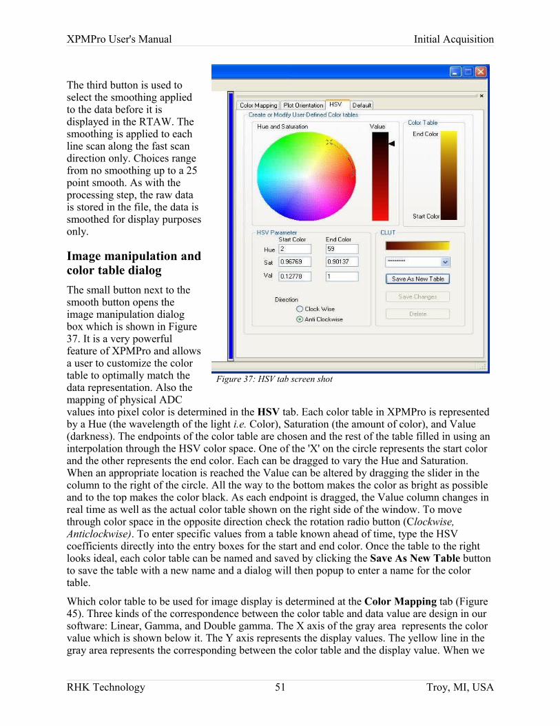
XPMPro User's Manual Initial Acquisition
The third button is used to select the smoothing applied to the data before it is displayed in the RTAW. The smoothing is applied to each line scan along the fast scan direction only. Choices range from no smoothing up to a 25 point smooth. As with the processing step, the raw data is stored in the file, the data is smoothed for display purposes only.
Image manipulation and color table dialogThe small button next to the smooth button opens the image manipulation dialog box which is shown in Figure37. It is a very powerful feature of XPMPro and allows a user to customize the color table to optimally match the data representation. Also the mapping of physical ADC values into pixel color is determined in the HSV tab. Each color table in XPMPro is represented by a Hue (the wavelength of the light i.e. Color), Saturation (the amount of color), and Value (darkness). The endpoints of the color table are chosen and the rest of the table filled in using an interpolation through the HSV color space. One of the 'X' on the circle represents the start color and the other represents the end color. Each can be dragged to vary the Hue and Saturation. When an appropriate location is reached the Value can be altered by dragging the slider in the column to the right of the circle. All the way to the bottom makes the color as bright as possible and to the top makes the color black. As each endpoint is dragged, the Value column changes in real time as well as the actual color table shown on the right side of the window. To move through color space in the opposite direction check the rotation radio button (Clockwise, Anticlockwise). To enter specific values from a table known ahead of time, type the HSV coefficients directly into the entry boxes for the start and end color. Once the table to the right looks ideal, each color table can be named and saved by clicking the Save As New Table button to save the table with a new name and a dialog will then popup to enter a name for the color table.
Which color table to be used for image display is determined at the Color Mapping tab (Figure45). Three kinds of the correspondence between the color table and data value are design in our software: Linear, Gamma, and Double gamma. The X axis of the gray area represents the color value which is shown below it. The Y axis represents the display values. The yellow line in the gray area represents the corresponding between the color table and the display value. When we
RHK Technology 51 Troy, MI, USA
Figure 37: HSV tab screen shot
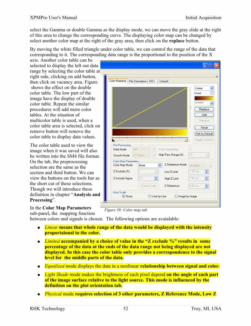
XPMPro User's Manual Initial Acquisition
select the Gamma or double Gamma as the display mode, we can move the gray slide at the right of this area to change the corresponding curve. The displaying color map can be changed by select another color map at the right of the gray area, then click on the replace button.
By moving the white filled triangle under color table, we can control the range of the data that corresponding to it. The corresponding data range is the proportional to the position of the X axis. Another color table can be selected to display the left out data range by selecting the color table at right side, clicking on add button, then click on vacancy area. Figure shows the effect on the double color table. The low part of the image have the display of double color table. Repeat the similar procedures will add more color tables. At the situation of multicolor table is used, when a color table area is selected, click on remove button will remove the color table to display data values.
The color table used to view the image when it was saved will also be written into the SM4 file format. On the tab, the preprocessing selection are the same as the section and third button. We can view the buttons on the tools bar as the short cut of these selections. Though we will introduce these definition in chapter “Analysis and Processing”.In the Color Map Parameters sub-panel, the mapping function between colors and signals is chosen. The following options are avaialable:
● Linear means that whole range of the data would be displayed with the intensity proportaional to the color.
● Limited accompanied by a choice of value in the “Z exclude %” results in some percentage of the data at the ends of the data range not being displayed are not displayed. In this case the color table only provides a correspondence to the signal level for the middle parts of the data.
● Equalized mode displays the data in a nonlinear relationship between signal and color.
● Light Shade mode makes the brightness of each pixel depend on the angle of each part of the image surface relative to the light source. This mode is influenced by the definition on the plot orientation tab.
● Physical mode requires selection of 3 other parameters, Z Reference Mode, Low Z
RHK Technology 52 Troy, MI, USA
Figure 38: Color map tab
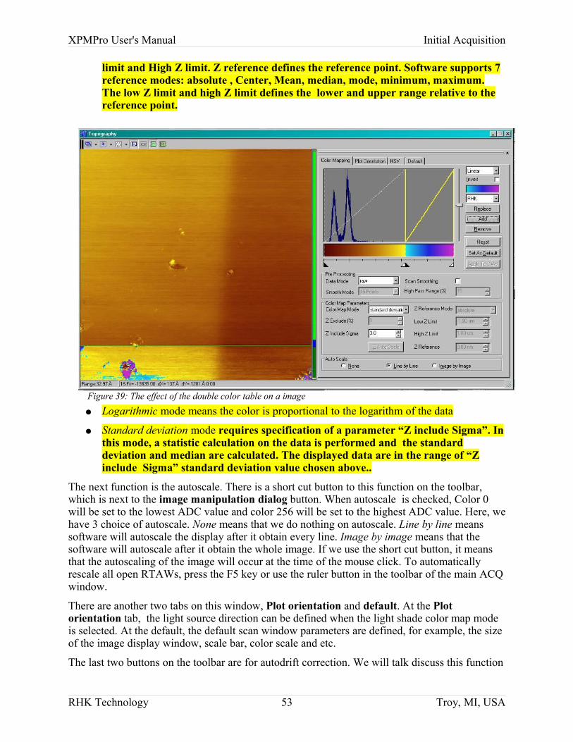
XPMPro User's Manual Initial Acquisition
limit and High Z limit. Z reference defines the reference point. Software supports 7 reference modes: absolute , Center, Mean, median, mode, minimum, maximum. The low Z limit and high Z limit defines the lower and upper range relative to the reference point.
● Logarithmic mode means the color is proportional to the logarithm of the data
● Standard deviation mode requires specification of a parameter “Z include Sigma”. In this mode, a statistic calculation on the data is performed and the standard deviation and median are calculated. The displayed data are in the range of “Z include Sigma” standard deviation value chosen above..
The next function is the autoscale. There is a short cut button to this function on the toolbar, which is next to the image manipulation dialog button. When autoscale is checked, Color 0 will be set to the lowest ADC value and color 256 will be set to the highest ADC value. Here, we have 3 choice of autoscale. None means that we do nothing on autoscale. Line by line means software will autoscale the display after it obtain every line. Image by image means that the software will autoscale after it obtain the whole image. If we use the short cut button, it means that the autoscaling of the image will occur at the time of the mouse click. To automatically rescale all open RTAWs, press the F5 key or use the ruler button in the toolbar of the main ACQ window.
There are another two tabs on this window, Plot orientation and default. At the Plot orientation tab, the light source direction can be defined when the light shade color map mode is selected. At the default, the default scan window parameters are defined, for example, the size of the image display window, scale bar, color scale and etc.
The last two buttons on the toolbar are for autodrift correction. We will talk discuss this function
RHK Technology 53 Troy, MI, USA
Figure 39: The effect of the double color table on a image
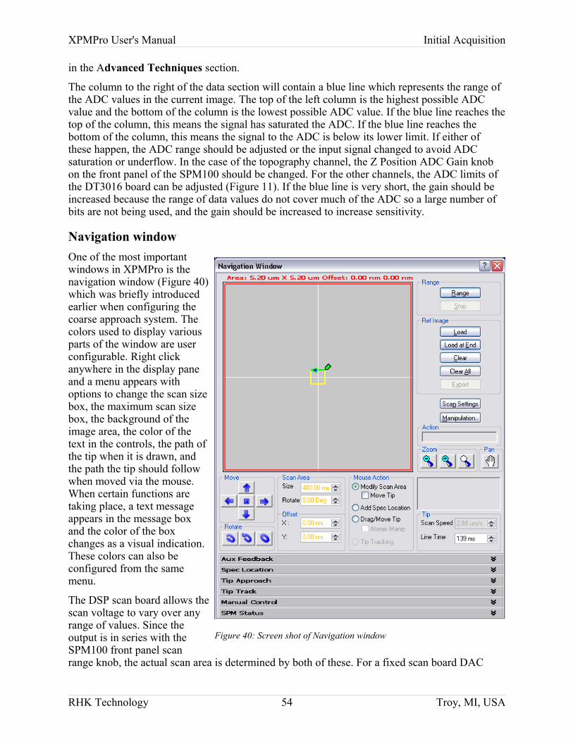
XPMPro User's Manual Initial Acquisition
in the Advanced Techniques section.
The column to the right of the data section will contain a blue line which represents the range of the ADC values in the current image. The top of the left column is the highest possible ADC value and the bottom of the column is the lowest possible ADC value. If the blue line reaches the top of the column, this means the signal has saturated the ADC. If the blue line reaches the bottom of the column, this means the signal to the ADC is below its lower limit. If either of these happen, the ADC range should be adjusted or the input signal changed to avoid ADC saturation or underflow. In the case of the topography channel, the Z Position ADC Gain knob on the front panel of the SPM100 should be changed. For the other channels, the ADC limits of the DT3016 board can be adjusted (Figure 11). If the blue line is very short, the gain should be increased because the range of data values do not cover much of the ADC so a large number of bits are not being used, and the gain should be increased to increase sensitivity.
Navigation windowOne of the most important windows in XPMPro is the navigation window (Figure 40) which was briefly introduced earlier when configuring the coarse approach system. The colors used to display various parts of the window are user configurable. Right click anywhere in the display pane and a menu appears with options to change the scan size box, the maximum scan size box, the background of the image area, the color of the text in the controls, the path of the tip when it is drawn, and the path the tip should follow when moved via the mouse. When certain functions are taking place, a text message appears in the message box and the color of the box changes as a visual indication. These colors can also be configured from the same menu.
The DSP scan board allows the scan voltage to vary over any range of values. Since the output is in series with the SPM100 front panel scan range knob, the actual scan area is determined by both of these. For a fixed scan board DAC
RHK Technology 54 Troy, MI, USA
Figure 40: Screen shot of Navigation window
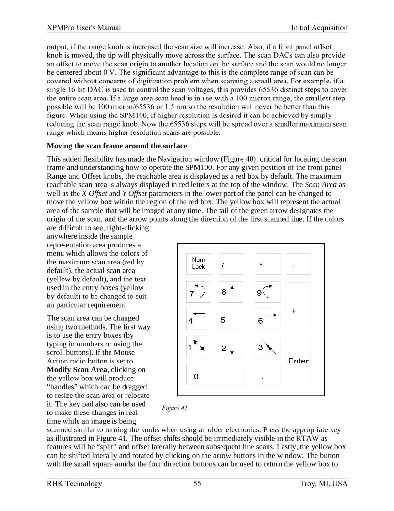
XPMPro User's Manual Initial Acquisition
output, if the range knob is increased the scan size will increase. Also, if a front panel offset knob is moved, the tip will physically move across the surface. The scan DACs can also provide an offset to move the scan origin to another location on the surface and the scan would no longer be centered about 0 V. The significant advantage to this is the complete range of scan can be covered without concerns of digitization problem when scanning a small area. For example, if a single 16 bit DAC is used to control the scan voltages, this provides 65536 distinct steps to cover the entire scan area. If a large area scan head is in use with a 100 micron range, the smallest step possible will be 100 micron/65536 or 1.5 nm so the resolution will never be better than this figure. When using the SPM100, if higher resolution is desired it can be achieved by simply reducing the scan range knob. Now the 65536 steps will be spread over a smaller maximum scan range which means higher resolution scans are possible.
Moving the scan frame around the surface
This added flexibility has made the Navigation window (Figure 40) critical for locating the scan frame and understanding how to operate the SPM100. For any given position of the front panel Range and Offset knobs, the reachable area is displayed as a red box by default. The maximum reachable scan area is always displayed in red letters at the top of the window. The Scan Area as well as the X Offset and Y Offset parameters in the lower part of the panel can be changed to move the yellow box within the region of the red box. The yellow box will represent the actual area of the sample that will be imaged at any time. The tail of the green arrow designates the origin of the scan, and the arrow points along the direction of the first scanned line. If the colors are difficult to see, right-clicking anywhere inside the sample representation area produces a menu which allows the colors of the maximum scan area (red by default), the actual scan area (yellow by default), and the text used in the entry boxes (yellow by default) to be changed to suit an particular requirement.
The scan area can be changed using two methods. The first way is to use the entry boxes (by typing in numbers or using the scroll buttons). If the Mouse Action radio button is set to Modify Scan Area, clicking on the yellow box will produce “handles” which can be dragged to resize the scan area or relocate it. The key pad also can be used to make these changes in real time while an image is being scanned similar to turning the knobs when using an older electronics. Press the appropriate key as illustrated in Figure 41. The offset shifts should be immediately visible in the RTAW as features will be “split” and offset laterally between subsequent line scans. Lastly, the yellow box can be shifted laterally and rotated by clicking on the arrow buttons in the window. The button with the small square amidst the four direction buttons can be used to return the yellow box to
RHK Technology 55 Troy, MI, USA
Figure 41

XPMPro User's Manual Initial Acquisition
the center of the red box which will set the two offset values to zero. Another option for moving the scan area laterally is to place the mouse where the scan are should be centered and click the right mouse button. A menu will appear and one choice is Move Scan Area Here. The scan area box will immediately move to this new position. When the mouse action is set to Modify Scan Area, moving the mouse cursor anywhere inside the maximum scan area (red box default color) will also display the location of the mouse at the top of the window. This is a quick method to record the physical coordinates of features in the window.
Anytime the scan area is changed when imaging is not taking place, the user has the option to have the tip follow the scan frame or leave the tip stationary and not move until imaging is started again. The second option avoids unnecessary tip motion, but the first option provides a simple method of moving the tip position small amounts across the surface if it always remains at a fixed position within the scan frame. To choose the first behavior )tip moves when box moves) make sure the Tip Motion box below the Modify Scan Area is checked.
The colors for the scan area frame, maximum scan area frame, background of the navigation area and text color of the scan area controls can all be changed to fit a user's preference. Each of these choices is accessed by right clicking anywhere in the navigation area and selecting the appropriate menu item.
The Load button in the Ref Image section allows the user to place any image in the scan area window for reference purposes. When clicking on this button, the cursor will change shape and a RTAW could be clicked or an image currently displayed in a data analysis window can be loaded. A large image can be acquired and then placed in the Navigation window in order to accurately reduce the scan frame to focus on a small object visible in the larger scan frame. The image is loaded as soon as a real time display window is selected, if the image is not completed a partial image is loaded and the rest of the image is filled in with null values. To ensure a complete image is loaded, either stop the scan at the end of the frame and then load the image or use the Load at End button. This selection will automatically load the selected image when it is completed and then the next frame acquisition will start.
The horizontal and vertical lines in the NAV window represent the center of the possible tip scan area (no piezo deflection) and are used as a reference to track how much tip motion there is when the front panel offset knobs are turned. When an image is loaded, the black lines indicate the center of the reference image. More than one image can be loaded at the same time and a panoramic view provided by many images combined together can be exported from the NAV window. Details for this function are described in the Advanced Techniques chapter.
The Zoom In and Zoom Out buttons (magnifying glass icon) are used to zoom in or zoom out the total area covered by the map. If the user wants to move the scan frame a very precise amount on an atomic scale to scan a specific feature, it would be best to zoom in quite a bit so the map area is rather small and the scan frame outline will be controlled very accurately with respect to the image loaded into the map. When zoomed in any level except maximum range, the Navigation window is centered on the yellow box. This also means as the scan frame is shifted, the yellow box appears stationary (since it remains centered) and the red box shifts opposite of the direction clicked making the net effect of moving the yellow box the desired direction. If the view is zoomed out as far as possible the view switches to centering on scanner zero. The magnifying glass with a white appearance next to the + and – buttons can be used to immediately return the zoom range to the maximum reachable scan area (like the scan range knob was turned all the way to 10). This can be useful to get a “bird's eye view” of the entire relative scan area if the red box and yellow box are both zoomed in quite a bit relative to the
RHK Technology 56 Troy, MI, USA
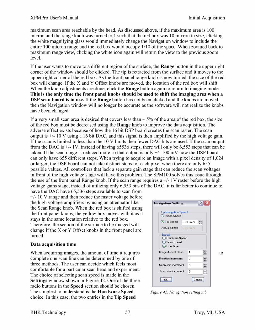
XPMPro User's Manual Initial Acquisition
maximum scan area reachable by the head. As discussed above, if the maximum area is 100 micron and the range knob was turned to 1 such that the red box was 10 micron in size, clicking the white magnifying glass would immediately change the Navigation window to include the entire 100 micron range and the red box would occupy 1/10 of the space. When zoomed back to maximum range view, clicking the white icon again will return the view to the previous zoom level.
If the user wants to move to a different region of the surface, the Range button in the upper right corner of the window should be clicked. The tip is retracted from the surface and it moves to the upper right corner of the red box. As the front panel range knob is now turned, the size of the red box will change. If the X and Y Offset knobs are moved, the location of the red box will shift. When the knob adjustments are done, click the Range button again to return to imaging mode. This is the only time the front panel knobs should be used to shift the imaging area when a DSP scan board is in use. If the Range button has not been clicked and the knobs are moved, then the Navigation window will no longer be accurate as the software will not realize the knobs have been changed.
If a very small scan area is desired that covers less than ~ 5% of the area of the red box, the size of the red box must be decreased using the Range knob to improve the data acquisition. The adverse effect exists because of how the 16 bit DSP board creates the scan raster. The scan output is +/- 10 V using a 16 bit DAC, and this signal is then amplified by the high voltage gain. If the scan is limited to less than the 10 V limits then fewer DAC bits are used. If the scan output from the DAC is +/- 1V, instead of having 65536 steps, there will only be 6,553 steps that can be taken. If the scan range is reduced more so that output is only +/- 100 mV now the DSP board can only have 655 different steps. When trying to acquire an image with a pixel density of 1,024 or larger, the DSP board can not take distinct steps for each pixel when there are only 655 possible values. All controllers that lack a separate gain stage that can reduce the scan voltages in front of the high voltage stage will have this problem. The SPM100 solves this issue through the use of the front panel Range knob. If the scan range requires a +/- 1V raster before the high voltage gains stage, instead of utilizing only 6,553 bits of the DAC, it is far better to continue to have the DAC have 65,536 steps available to scan from +/- 10 V range and then reduce the raster voltage before the high voltage amplifiers by using an attenuator like the Scan Range knob. When the red box is shifted using the front panel knobs, the yellow box moves with it as it stays in the same location relative to the red box. Therefore, the section of the surface to be imaged will change if the X or Y Offset knobs in the front panel are turned.
Data acquisition time
When acquiring images, the amount of time it requires to complete one scan line can be determined by one of three methods. The user can decide which feels most comfortable for a particular scan head and experiment. The choice of selecting scan speed is made in the Settings window shown in Figure 42. One of the three radio buttons in the Speed section should be chosen. The simplest to understand is the Hardware Speed choice. In this case, the two entries in the Tip Speed
RHK Technology 57 Troy, MI, USA
Figure 42: Navigation setting tab
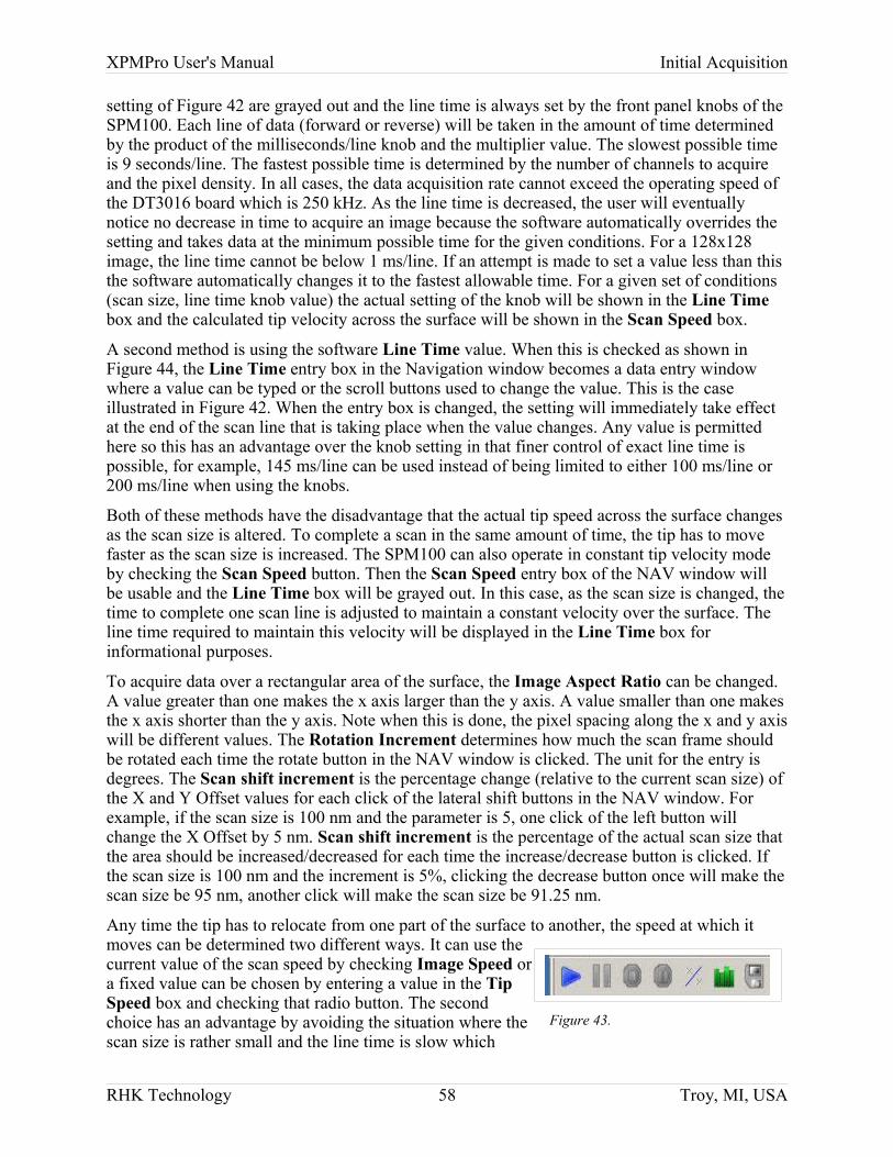
XPMPro User's Manual Initial Acquisition
setting of Figure 42 are grayed out and the line time is always set by the front panel knobs of the SPM100. Each line of data (forward or reverse) will be taken in the amount of time determined by the product of the milliseconds/line knob and the multiplier value. The slowest possible time is 9 seconds/line. The fastest possible time is determined by the number of channels to acquire and the pixel density. In all cases, the data acquisition rate cannot exceed the operating speed of the DT3016 board which is 250 kHz. As the line time is decreased, the user will eventually notice no decrease in time to acquire an image because the software automatically overrides the setting and takes data at the minimum possible time for the given conditions. For a 128x128 image, the line time cannot be below 1 ms/line. If an attempt is made to set a value less than this the software automatically changes it to the fastest allowable time. For a given set of conditions (scan size, line time knob value) the actual setting of the knob will be shown in the Line Time box and the calculated tip velocity across the surface will be shown in the Scan Speed box.
A second method is using the software Line Time value. When this is checked as shown in Figure 44, the Line Time entry box in the Navigation window becomes a data entry window where a value can be typed or the scroll buttons used to change the value. This is the case illustrated in Figure 42. When the entry box is changed, the setting will immediately take effect at the end of the scan line that is taking place when the value changes. Any value is permitted here so this has an advantage over the knob setting in that finer control of exact line time is possible, for example, 145 ms/line can be used instead of being limited to either 100 ms/line or 200 ms/line when using the knobs.
Both of these methods have the disadvantage that the actual tip speed across the surface changes as the scan size is altered. To complete a scan in the same amount of time, the tip has to move faster as the scan size is increased. The SPM100 can also operate in constant tip velocity mode by checking the Scan Speed button. Then the Scan Speed entry box of the NAV window will be usable and the Line Time box will be grayed out. In this case, as the scan size is changed, the time to complete one scan line is adjusted to maintain a constant velocity over the surface. The line time required to maintain this velocity will be displayed in the Line Time box for informational purposes.
To acquire data over a rectangular area of the surface, the Image Aspect Ratio can be changed. A value greater than one makes the x axis larger than the y axis. A value smaller than one makes the x axis shorter than the y axis. Note when this is done, the pixel spacing along the x and y axis will be different values. The Rotation Increment determines how much the scan frame should be rotated each time the rotate button in the NAV window is clicked. The unit for the entry is degrees. The Scan shift increment is the percentage change (relative to the current scan size) of the X and Y Offset values for each click of the lateral shift buttons in the NAV window. For example, if the scan size is 100 nm and the parameter is 5, one click of the left button will change the X Offset by 5 nm. Scan shift increment is the percentage of the actual scan size that the area should be increased/decreased for each time the increase/decrease button is clicked. If the scan size is 100 nm and the increment is 5%, clicking the decrease button once will make the scan size be 95 nm, another click will make the scan size be 91.25 nm.
Any time the tip has to relocate from one part of the surface to another, the speed at which it moves can be determined two different ways. It can use the current value of the scan speed by checking Image Speed or a fixed value can be chosen by entering a value in the Tip Speed box and checking that radio button. The second choice has an advantage by avoiding the situation where the scan size is rather small and the line time is slow which
RHK Technology 58 Troy, MI, USA
Figure 43.
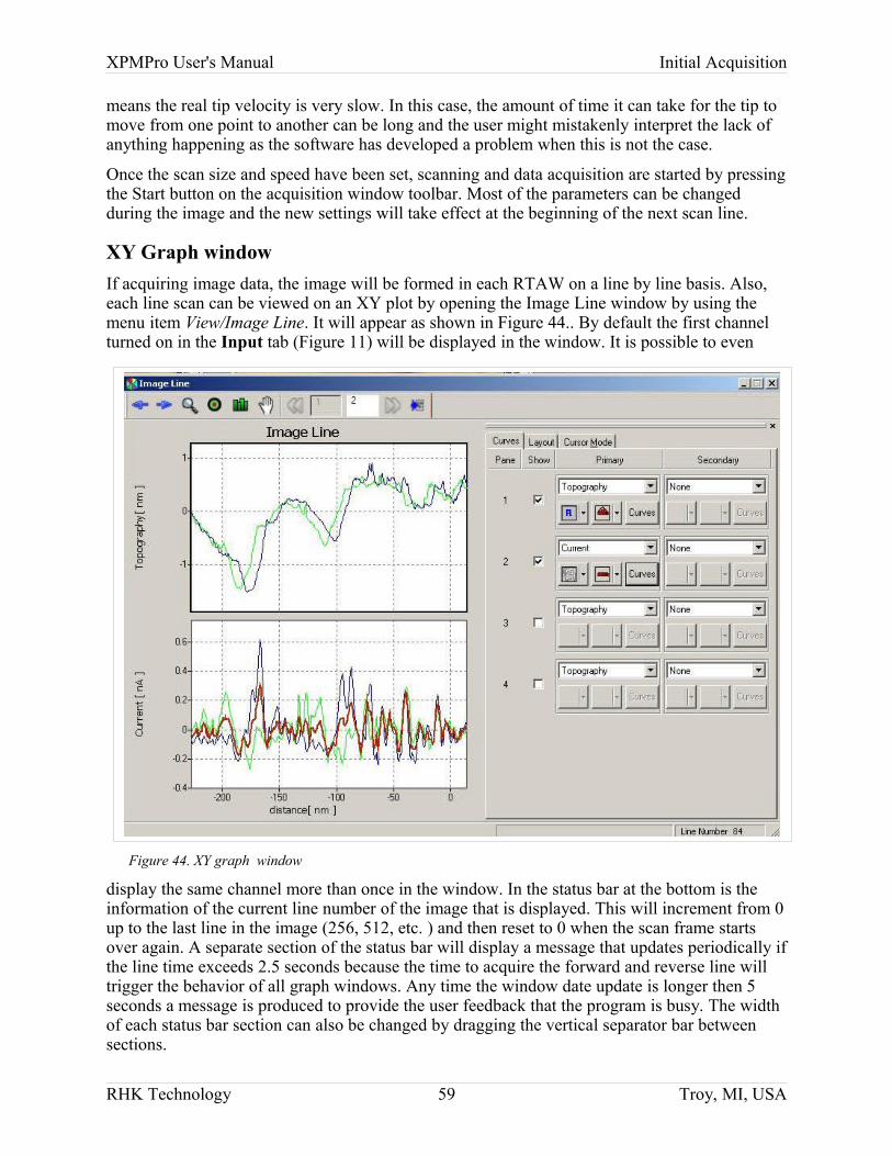
XPMPro User's Manual Initial Acquisition
means the real tip velocity is very slow. In this case, the amount of time it can take for the tip to move from one point to another can be long and the user might mistakenly interpret the lack of anything happening as the software has developed a problem when this is not the case.
Once the scan size and speed have been set, scanning and data acquisition are started by pressing the Start button on the acquisition window toolbar. Most of the parameters can be changed during the image and the new settings will take effect at the beginning of the next scan line.
XY Graph windowIf acquiring image data, the image will be formed in each RTAW on a line by line basis. Also, each line scan can be viewed on an XY plot by opening the Image Line window by using the menu item View/Image Line. It will appear as shown in Figure 44.. By default the first channel turned on in the Input tab (Figure 11) will be displayed in the window. It is possible to even
display the same channel more than once in the window. In the status bar at the bottom is the information of the current line number of the image that is displayed. This will increment from 0 up to the last line in the image (256, 512, etc. ) and then reset to 0 when the scan frame starts over again. A separate section of the status bar will display a message that updates periodically if the line time exceeds 2.5 seconds because the time to acquire the forward and reverse line will trigger the behavior of all graph windows. Any time the window date update is longer then 5 seconds a message is produced to provide the user feedback that the program is busy. The width of each status bar section can also be changed by dragging the vertical separator bar between sections.
RHK Technology 59 Troy, MI, USA
Figure 44. XY graph window
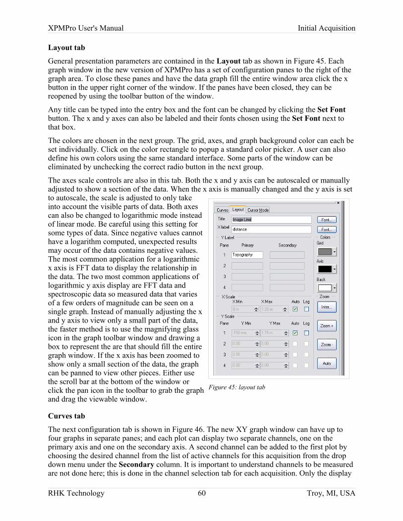
XPMPro User's Manual Initial Acquisition
Layout tab
General presentation parameters are contained in the Layout tab as shown in Figure 45. Each graph window in the new version of XPMPro has a set of configuration panes to the right of the graph area. To close these panes and have the data graph fill the entire window area click the x button in the upper right corner of the window. If the panes have been closed, they can be reopened by using the toolbar button of the window.
Any title can be typed into the entry box and the font can be changed by clicking the Set Font button. The x and y axes can also be labeled and their fonts chosen using the Set Font next to that box.
The colors are chosen in the next group. The grid, axes, and graph background color can each be set individually. Click on the color rectangle to popup a standard color picker. A user can also define his own colors using the same standard interface. Some parts of the window can be eliminated by unchecking the correct radio button in the next group.
The axes scale controls are also in this tab. Both the x and y axis can be autoscaled or manually adjusted to show a section of the data. When the x axis is manually changed and the y axis is set to autoscale, the scale is adjusted to only take into account the visible parts of data. Both axes can also be changed to logarithmic mode instead of linear mode. Be careful using this setting for some types of data. Since negative values cannot have a logarithm computed, unexpected results may occur of the data contains negative values. The most common application for a logarithmic x axis is FFT data to display the relationship in the data. The two most common applications of logarithmic y axis display are FFT data and spectroscopic data so measured data that varies of a few orders of magnitude can be seen on a single graph. Instead of manually adjusting the x and y axis to view only a small part of the data, the faster method is to use the magnifying glass icon in the graph toolbar window and drawing a box to represent the are that should fill the entire graph window. If the x axis has been zoomed to show only a small section of the data, the graph can be panned to view other pieces. Either use the scroll bar at the bottom of the window or click the pan icon in the toolbar to grab the graph and drag the viewable window.
Curves tab
The next configuration tab is shown in Figure 46. The new XY graph window can have up to four graphs in separate panes; and each plot can display two separate channels, one on the primary axis and one on the secondary axis. A second channel can be added to the first plot by choosing the desired channel from the list of active channels for this acquisition from the drop down menu under the Secondary column. It is important to understand channels to be measured are not done here; this is done in the channel selection tab for each acquisition. Only the display
RHK Technology 60 Troy, MI, USA
Figure 45: layout tab
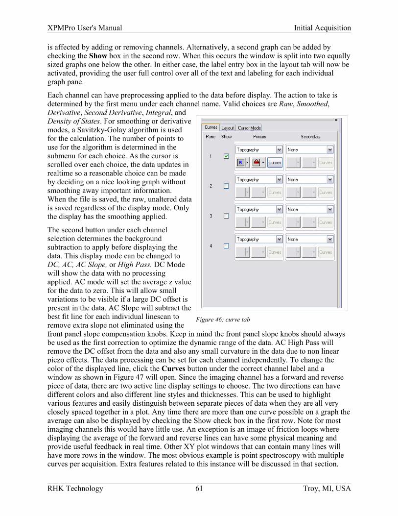
XPMPro User's Manual Initial Acquisition
is affected by adding or removing channels. Alternatively, a second graph can be added by checking the Show box in the second row. When this occurs the window is split into two equally sized graphs one below the other. In either case, the label entry box in the layout tab will now be activated, providing the user full control over all of the text and labeling for each individual graph pane.
Each channel can have preprocessing applied to the data before display. The action to take is determined by the first menu under each channel name. Valid choices are Raw, Smoothed, Derivative, Second Derivative, Integral, and Density of States. For smoothing or derivative modes, a Savitzky-Golay algorithm is used for the calculation. The number of points to use for the algorithm is determined in the submenu for each choice. As the cursor is scrolled over each choice, the data updates in realtime so a reasonable choice can be made by deciding on a nice looking graph without smoothing away important information. When the file is saved, the raw, unaltered data is saved regardless of the display mode. Only the display has the smoothing applied.
The second button under each channel selection determines the background subtraction to apply before displaying the data. This display mode can be changed to DC, AC, AC Slope, or High Pass. DC Mode will show the data with no processing applied. AC mode will set the average z value for the data to zero. This will allow small variations to be visible if a large DC offset is present in the data. AC Slope will subtract the best fit line for each individual linescan to remove extra slope not eliminated using the front panel slope compensation knobs. Keep in mind the front panel slope knobs should always be used as the first correction to optimize the dynamic range of the data. AC High Pass will remove the DC offset from the data and also any small curvature in the data due to non linear piezo effects. The data processing can be set for each channel independently. To change the color of the displayed line, click the Curves button under the correct channel label and a window as shown in Figure 47 will open. Since the imaging channel has a forward and reverse piece of data, there are two active line display settings to choose. The two directions can have different colors and also different line styles and thicknesses. This can be used to highlight various features and easily distinguish between separate pieces of data when they are all very closely spaced together in a plot. Any time there are more than one curve possible on a graph the average can also be displayed by checking the Show check box in the first row. Note for most imaging channels this would have little use. An exception is an image of friction loops where displaying the average of the forward and reverse lines can have some physical meaning and provide useful feedback in real time. Other XY plot windows that can contain many lines will have more rows in the window. The most obvious example is point spectroscopy with multiple curves per acquisition. Extra features related to this instance will be discussed in that section.
RHK Technology 61 Troy, MI, USA
Figure 46: curve tab
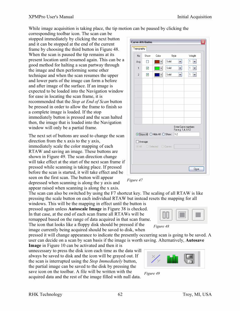
XPMPro User's Manual Initial Acquisition
While image acquisition is taking place, the tip motion can be paused by clicking the corresponding toolbar icon. The scan can be stopped immediately by clicking the next button and it can be stopped at the end of the current frame by choosing the third button in Figure 48. When the scan is paused the tip remains at its present location until resumed again. This can be a good method for halting a scan partway through the image and then performing some other technique and when the scan resumes the upper and lower parts of the image can form a before and after image of the surface. If an image is expected to be loaded into the Navigation window for ease in locating the scan frame, it is recommended that the Stop at End of Scan button be pressed in order to allow the frame to finish so a complete image is loaded. If the stop immediately button is pressed and the scan halted then, the image that is loaded into the Navigation window will only be a partial frame.
The next set of buttons are used to change the scan direction from the x axis to the y axis, immediately scale the color mapping of each RTAW and saving an image. These buttons are shown in Figure 49. The scan direction change will take effect at the start of the next scan frame if pressed while scanning is taking place. If pressed before the scan is started, it will take effect and be seen on the first scan. The button will appear depressed when scanning is along the y axis and appear raised when scanning is along the x axis. The scan can also be switched by using the F7 shortcut key. The scaling of all RTAW is like pressing the scale button on each individual RTAW but instead resets the mapping for all windows. This will be the mapping in effect until the button is pressed again unless Autoscale Image in Figure 38 is checked. In that case, at the end of each scan frame all RTAWs will be remapped based on the range of data acquired in that scan frame. The icon that looks like a floppy disk should be pressed if the image currently being acquired should be saved to disk, when pressed it will change appearance to indicate the presently occurring scan is going to be saved. A user can decide on a scan by scan basis if the image is worth saving. Alternatively, Autosave Image in Figure 10 can be activated and then it is unnecessary to press the disk icon each time as the data will always be saved to disk and the icon will be grayed out. If the scan is interrupted using the Stop Immediately button, the partial image can be saved to the disk by pressing the save icon on the toolbar. A file will be written with the acquired data and the rest of the image filled with null data.
RHK Technology 62 Troy, MI, USA
Figure 47
Figure 49
Figure 48
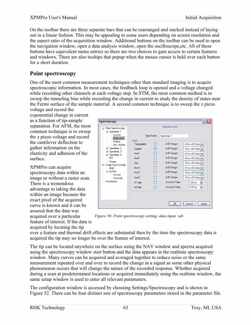
XPMPro User's Manual Initial Acquisition
On the toolbar there are three separate bars that can be rearranged and stacked instead of laying out in a linear fashion. This may be appealing to some users depending on screen resolution and the aspect ratio of the acquisition window. Additional buttons on the toolbar can be used to open the navigation window, open a data analysis window, open the oscilloscope,etc. All of these buttons have equivalent menu entries so there are two choices to gain access to certain features and windows. There are also tooltips that popup when the mouse cursor is held over each button for a short duration.
Point spectroscopyOne of the most common measurement techniques other than standard imaging is to acquire spectroscopic information. In most cases, the feedback loop is opened and a voltage changed while recording other channels at each voltage step. In STM, the most common method is to sweep the tunneling bias while recording the change in current to study the density of states near the Fermi surface of the sample material. A second common technique is to sweep the z piezo voltage and record the exponential change in current as a function of tip-sample separation. For AFM, the most common technique is to sweep the z piezo voltage and record the cantilever deflection to gather information on the elasticity and adhesion of the surface.
XPMPro can acquire spectroscopy data within an image or without a raster scan. There is a tremendous advantage to taking the data within an image because the exact pixel of the acquired curve is known and it can be assured that the data was acquired over a particular feature of interest. If the data is acquired by locating the tip over a feature and thermal drift effects are substantial then by the time the spectroscopy data is acquired the tip may no longer be over the feature of interest.
The tip can be located anywhere on the surface using the NAV window and spectra acquired using the spectroscopy window start button and the data appears in the realtime spectroscopy window. Many curves can be acquired and averaged together to reduce noise or the same measurement repeated over and over to record the change in a signal as some other physical phenomenon occurs that will change the nature of the recorded response. Whether acquired during a scan at predetermined locations or acquired immediately using the realtime window, the same setup window is used to enter all relevant parameters.
The configuration window is accessed by choosing Settings/Spectroscopy and is shown in Figure 52. There can be four distinct sets of spectroscopy parameters stored in the parameter file.
RHK Technology 63 Troy, MI, USA
Figure 50: Point spectroscopy setting- data input tab
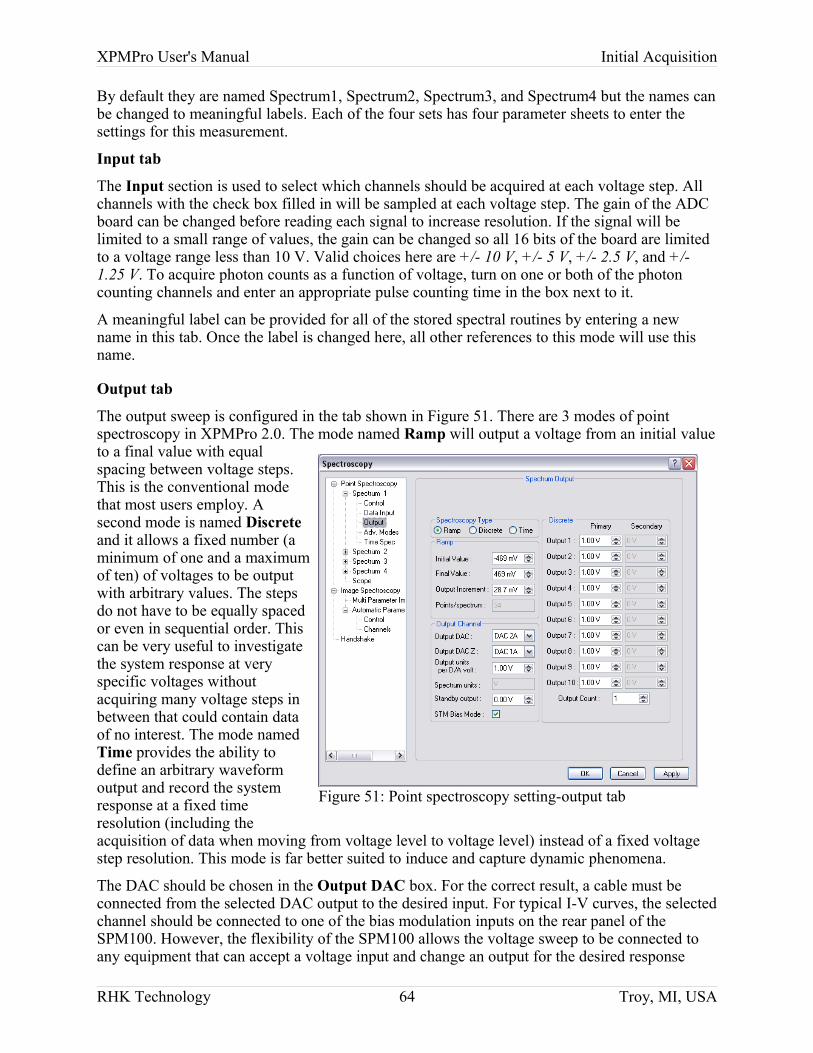
XPMPro User's Manual Initial Acquisition
By default they are named Spectrum1, Spectrum2, Spectrum3, and Spectrum4 but the names can be changed to meaningful labels. Each of the four sets has four parameter sheets to enter the settings for this measurement.
Input tab
The Input section is used to select which channels should be acquired at each voltage step. All channels with the check box filled in will be sampled at each voltage step. The gain of the ADC board can be changed before reading each signal to increase resolution. If the signal will be limited to a small range of values, the gain can be changed so all 16 bits of the board are limited to a voltage range less than 10 V. Valid choices here are +/- 10 V, +/- 5 V, +/- 2.5 V, and +/- 1.25 V. To acquire photon counts as a function of voltage, turn on one or both of the photon counting channels and enter an appropriate pulse counting time in the box next to it.
A meaningful label can be provided for all of the stored spectral routines by entering a new name in this tab. Once the label is changed here, all other references to this mode will use this name.
Output tab
The output sweep is configured in the tab shown in Figure 51. There are 3 modes of point spectroscopy in XPMPro 2.0. The mode named Ramp will output a voltage from an initial value to a final value with equal spacing between voltage steps. This is the conventional mode that most users employ. A second mode is named Discrete and it allows a fixed number (a minimum of one and a maximum of ten) of voltages to be output with arbitrary values. The steps do not have to be equally spaced or even in sequential order. This can be very useful to investigate the system response at very specific voltages without acquiring many voltage steps in between that could contain data of no interest. The mode named Time provides the ability to define an arbitrary waveform output and record the system response at a fixed time resolution (including the acquisition of data when moving from voltage level to voltage level) instead of a fixed voltage step resolution. This mode is far better suited to induce and capture dynamic phenomena.
The DAC should be chosen in the Output DAC box. For the correct result, a cable must be connected from the selected DAC output to the desired input. For typical I-V curves, the selected channel should be connected to one of the bias modulation inputs on the rear panel of the SPM100. However, the flexibility of the SPM100 allows the voltage sweep to be connected to any equipment that can accept a voltage input and change an output for the desired response
RHK Technology 64 Troy, MI, USA
Figure 51: Point spectroscopy setting-output tab
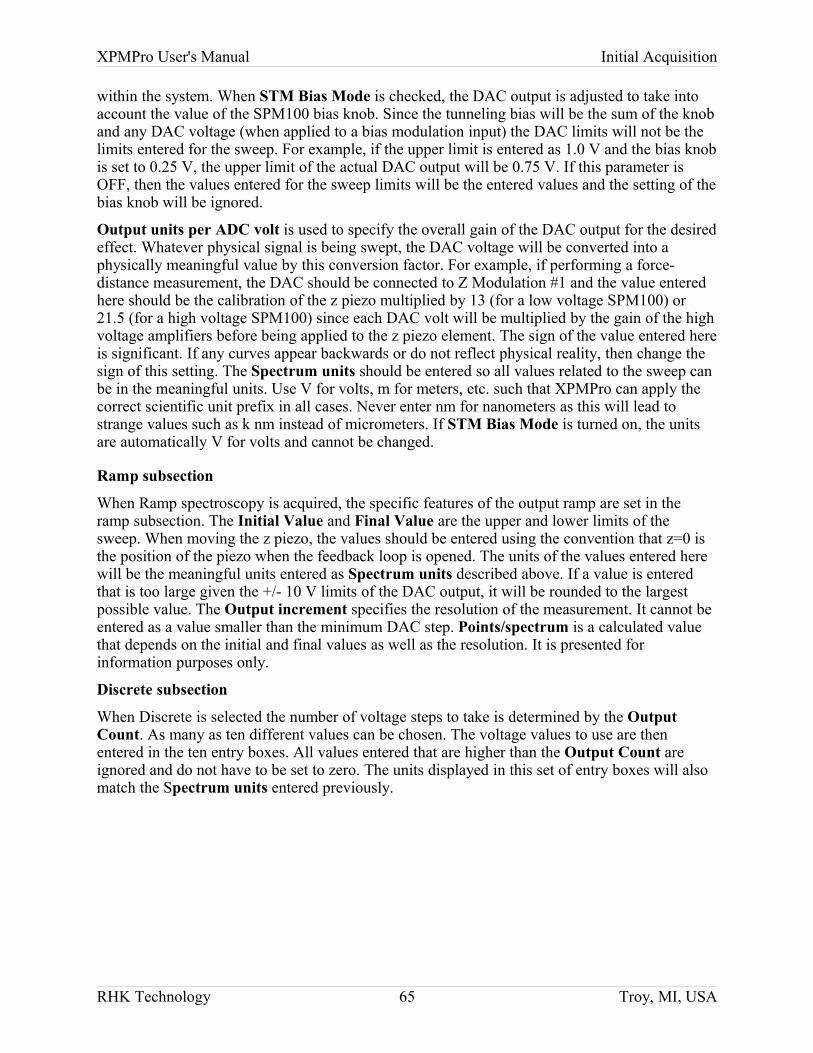
XPMPro User's Manual Initial Acquisition
within the system. When STM Bias Mode is checked, the DAC output is adjusted to take into account the value of the SPM100 bias knob. Since the tunneling bias will be the sum of the knob and any DAC voltage (when applied to a bias modulation input) the DAC limits will not be the limits entered for the sweep. For example, if the upper limit is entered as 1.0 V and the bias knob is set to 0.25 V, the upper limit of the actual DAC output will be 0.75 V. If this parameter is OFF, then the values entered for the sweep limits will be the entered values and the setting of the bias knob will be ignored.
Output units per ADC volt is used to specify the overall gain of the DAC output for the desired effect. Whatever physical signal is being swept, the DAC voltage will be converted into a physically meaningful value by this conversion factor. For example, if performing a force-distance measurement, the DAC should be connected to Z Modulation #1 and the value entered here should be the calibration of the z piezo multiplied by 13 (for a low voltage SPM100) or 21.5 (for a high voltage SPM100) since each DAC volt will be multiplied by the gain of the high voltage amplifiers before being applied to the z piezo element. The sign of the value entered here is significant. If any curves appear backwards or do not reflect physical reality, then change the sign of this setting. The Spectrum units should be entered so all values related to the sweep can be in the meaningful units. Use V for volts, m for meters, etc. such that XPMPro can apply the correct scientific unit prefix in all cases. Never enter nm for nanometers as this will lead to strange values such as k nm instead of micrometers. If STM Bias Mode is turned on, the units are automatically V for volts and cannot be changed.
Ramp subsection
When Ramp spectroscopy is acquired, the specific features of the output ramp are set in the ramp subsection. The Initial Value and Final Value are the upper and lower limits of the sweep. When moving the z piezo, the values should be entered using the convention that z=0 is the position of the piezo when the feedback loop is opened. The units of the values entered here will be the meaningful units entered as Spectrum units described above. If a value is entered that is too large given the +/- 10 V limits of the DAC output, it will be rounded to the largest possible value. The Output increment specifies the resolution of the measurement. It cannot be entered as a value smaller than the minimum DAC step. Points/spectrum is a calculated value that depends on the initial and final values as well as the resolution. It is presented for information purposes only.
Discrete subsection
When Discrete is selected the number of voltage steps to take is determined by the Output Count. As many as ten different values can be chosen. The voltage values to use are then entered in the ten entry boxes. All values entered that are higher than the Output Count are ignored and do not have to be set to zero. The units displayed in this set of entry boxes will also match the Spectrum units entered previously.
RHK Technology 65 Troy, MI, USA
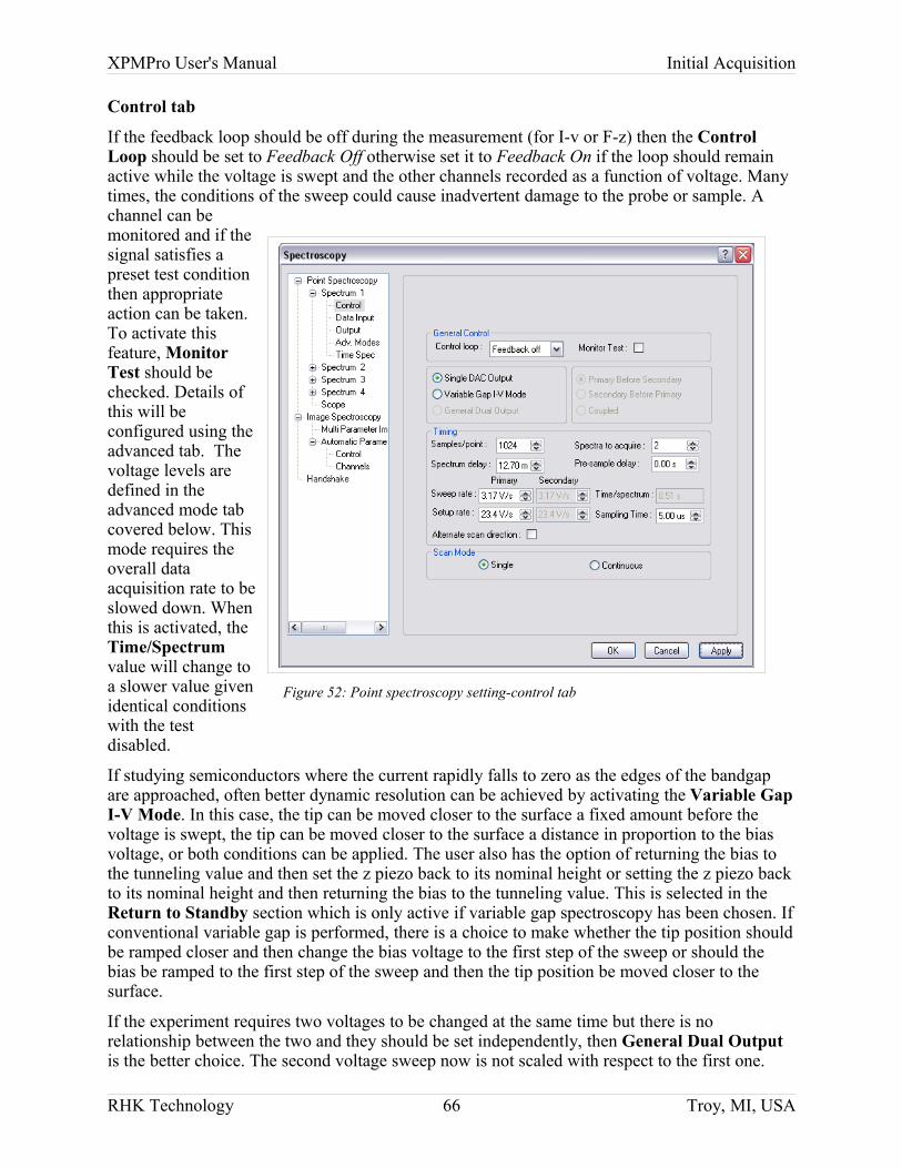
XPMPro User's Manual Initial Acquisition
Control tab
If the feedback loop should be off during the measurement (for I-v or F-z) then the Control Loop should be set to Feedback Off otherwise set it to Feedback On if the loop should remain active while the voltage is swept and the other channels recorded as a function of voltage. Many times, the conditions of the sweep could cause inadvertent damage to the probe or sample. A channel can be monitored and if the signal satisfies a preset test condition then appropriate action can be taken. To activate this feature, Monitor Test should be checked. Details of this will be configured using the advanced tab. The voltage levels are defined in the advanced mode tab covered below. This mode requires the overall data acquisition rate to be slowed down. When this is activated, the Time/Spectrum value will change to a slower value given identical conditions with the test disabled.
If studying semiconductors where the current rapidly falls to zero as the edges of the bandgap are approached, often better dynamic resolution can be achieved by activating the Variable Gap I-V Mode. In this case, the tip can be moved closer to the surface a fixed amount before the voltage is swept, the tip can be moved closer to the surface a distance in proportion to the bias voltage, or both conditions can be applied. The user also has the option of returning the bias to the tunneling value and then set the z piezo back to its nominal height or setting the z piezo back to its nominal height and then returning the bias to the tunneling value. This is selected in the Return to Standby section which is only active if variable gap spectroscopy has been chosen. If conventional variable gap is performed, there is a choice to make whether the tip position should be ramped closer and then change the bias voltage to the first step of the sweep or should the bias be ramped to the first step of the sweep and then the tip position be moved closer to the surface.
If the experiment requires two voltages to be changed at the same time but there is no relationship between the two and they should be set independently, then General Dual Output is the better choice. The second voltage sweep now is not scaled with respect to the first one.
RHK Technology 66 Troy, MI, USA
Figure 52: Point spectroscopy setting-control tab
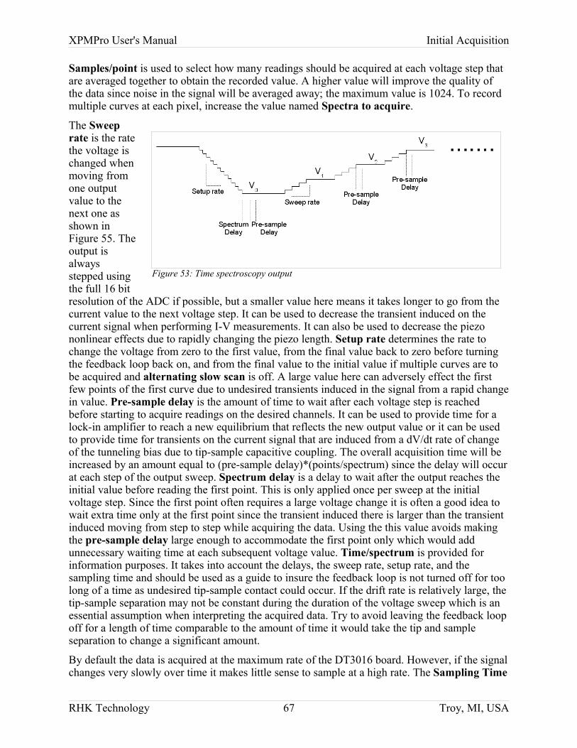
XPMPro User's Manual Initial Acquisition
Samples/point is used to select how many readings should be acquired at each voltage step that are averaged together to obtain the recorded value. A higher value will improve the quality of the data since noise in the signal will be averaged away; the maximum value is 1024. To record multiple curves at each pixel, increase the value named Spectra to acquire.
The Sweep rate is the rate the voltage is changed when moving from one output value to the next one as shown in Figure 55. The output is always stepped using the full 16 bit resolution of the ADC if possible, but a smaller value here means it takes longer to go from the current value to the next voltage step. It can be used to decrease the transient induced on the current signal when performing I-V measurements. It can also be used to decrease the piezo nonlinear effects due to rapidly changing the piezo length. Setup rate determines the rate to change the voltage from zero to the first value, from the final value back to zero before turning the feedback loop back on, and from the final value to the initial value if multiple curves are to be acquired and alternating slow scan is off. A large value here can adversely effect the first few points of the first curve due to undesired transients induced in the signal from a rapid change in value. Pre-sample delay is the amount of time to wait after each voltage step is reached before starting to acquire readings on the desired channels. It can be used to provide time for a lock-in amplifier to reach a new equilibrium that reflects the new output value or it can be used to provide time for transients on the current signal that are induced from a dV/dt rate of change of the tunneling bias due to tip-sample capacitive coupling. The overall acquisition time will be increased by an amount equal to (pre-sample delay)*(points/spectrum) since the delay will occur at each step of the output sweep. Spectrum delay is a delay to wait after the output reaches the initial value before reading the first point. This is only applied once per sweep at the initial voltage step. Since the first point often requires a large voltage change it is often a good idea to wait extra time only at the first point since the transient induced there is larger than the transient induced moving from step to step while acquiring the data. Using the this value avoids making the pre-sample delay large enough to accommodate the first point only which would add unnecessary waiting time at each subsequent voltage value. Time/spectrum is provided for information purposes. It takes into account the delays, the sweep rate, setup rate, and the sampling time and should be used as a guide to insure the feedback loop is not turned off for too long of a time as undesired tip-sample contact could occur. If the drift rate is relatively large, the tip-sample separation may not be constant during the duration of the voltage sweep which is an essential assumption when interpreting the acquired data. Try to avoid leaving the feedback loop off for a length of time comparable to the amount of time it would take the tip and sample separation to change a significant amount.
By default the data is acquired at the maximum rate of the DT3016 board. However, if the signal changes very slowly over time it makes little sense to sample at a high rate. The Sampling Time
RHK Technology 67 Troy, MI, USA
Figure 53: Time spectroscopy output
XPMPro User's Manual Initial Acquisition
can be used to spread out the samples so averaging of the readings makes more sense. If using a lockin amplifier with a time constant longer than 5 microseconds it is desirable to read the data at a rate slower than the time constant setting and this can be accomplished by altering the Sampling Time. Keep in mind when slowing down the ADC subsystem to spread out the readings, the DAC subsystem is also slowed down to maintain synchronization. This means for a given sweep rate the DAC may have to produce steps larger than the LSB in order to reach the next voltage level within the time interval defined by the sweep rate. When Alternate scan direction is checked, the first curve is swept from the initial value to the final value and the second curve is acquired while being swept from the final value back to the initial value. This is the required method to obtain force distance curves in AFM and can also be used to measure the amount of capacitive coupling between the tip and sample when the tunneling bias is swept. When this is on, the Spectra to acquire will always be entered as an even number to obtain pairs of curves.
To automatically have every set of curves written to the disk when using the realtime spectroscopy window, turn on Spectrum Autosave. The files will be named according to the autonaming convention specified in the Settings/Scan/Save tab. If autosave is off, then any set of curves that are acquired when using the spectroscopy start button are lost unless the Save button is pressed during the sweep (or after the sweep if it is stopped). When acquiring spectra within an image, they are saved in the same manner that applies to saving image files, and this parameter is ignored. Scan mode determines if the specified acquisition occurs only once and stopped if the spectral acquisition is repeated over and over until manually stopped with the toolbar button. This only applies when acquiring spectroscopy using the realtime spectroscopy window and the spectroscopy start button. When acquiring spectra within an image, the acquisition setup is only run once per pixel location.
Two acquisition modes can be used if acquiring instantaneous spectral data NOT during an image scan. Either Single can be chosen which means the the number of curves specified by Spectra to Acquire are measured and then the sweep stops, or Continuous can be chosen which means the measurement is performed Spectra to Acquire number of times and then that data either saved or thrown away and the routine started again. This will continue indefinitely until stopped by user interaction. The two modes are analogous to image acquisition where the Scan Count parameter in Figure 9 can be set to zero for free scanning until stopped or the specified number of images are acquired and then the scanning automatically stops.
Advanced modes tab
In the last tab, some of the sophisticated features of the spectroscopy routine can be configured. The parameters in the Monitor Mode and Variable Gap Mode sections will be ignored unless specifically activated for the routine.
If the spectroscopy routine needs to be synchronized with external equipment of some sort, the Handshaking routine can be called during each sweep. The conditions of the handshake are configured in the handshake tab in this same window as shown in Figure 54. It will be covered in detail later. While data is being acquired, the realtime spectroscopy window will be present on the screen and the curves will be drawn on the graph as they are acquired. The graphics overhead for this capability may slow down the actual acquisition rate in some cases. To make sure the data is acquired as quickly as possible, the Suppress inline graphics updates box can be checked. Then the curve will be drawn after the sweep has reached the final spectroscopy value and all data for that sweep has been read.
RHK Technology 68 Troy, MI, USA
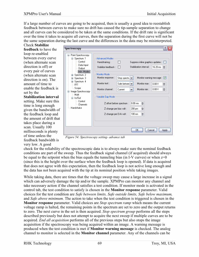
XPMPro User's Manual Initial Acquisition
If a large number of curves are going to be acquired, then is usually a good idea to reestablish feedback between curves to make sure no drift has caused the tip-sample separation to change and all curves can be considered to be taken at the same conditions. If the drift rate is significant over the time it takes to acquire all curves, then the separation during the first curve will not be the same separation during the last curve and the differences in the data may be misinterpreted. Check Stabilize feedback to have the loop re-enabled between every curve (when alternate scan direction is off) or every pair of curves (when alternate scan direction is on). The amount of time to enable the feedback is set by the Stabilization interval setting. Make sure this time is long enough given the bandwidth of the feedback loop and the amount of drift that takes place during a scan. Usually 100 milliseconds is plenty of time unless the feedback bandwidth is very low. A good check for the reliability of the spectroscopic data is to always make sure the nominal feedback conditions are part of the sweep. Thus the feedback signal channel (if acquired) should always be equal to the setpoint when the bias equals the tunneling bias (in I-V curves) or when z=0 (since this is the height over the surface when the feedback loop is opened). If data is acquired that does not agree with this expectation, then the feedback loop is not active long enough and the data has not been acquired with the tip at its nominal position while taking images.
While taking data, there are times that the voltage sweep may cause a large increase in a signal which can adversely damage the tip and/or the sample. XPMPro can monitor any channel and take necessary action if the channel satisfies a test condition. If monitor mode is activated in the control tab, the test condition to satisfy is chosen in the Monitor response parameter. Valid choices for the test condition are Safe between limits, Safe outside limits, Safe below maximum, and Safe above minimum. The action to take when the test condition is triggered is chosen in the Monitor response parameter. Valid choices are Stop spectrum ramp which means the current voltage ramp is halted, the remaining points in the spectrum are set to zero and the output returns to zero. The next curve in the set is then acquired. Stop spectrum group performs all the steps described previously but does not attempt to acquire the next sweep if multiple curves are to be acquired. End all acquisition performs all of the previous steps but also stops the image acquisition if the spectroscopy was being acquired within an image. A warning message is produced when the test condition is met if Monitor warning message is checked. The analog channel to monitor is selected in the Monitor channel parameter. Any of the channels can be
RHK Technology 69 Troy, MI, USA
Figure 54: Spectroscopy setting- advance tab
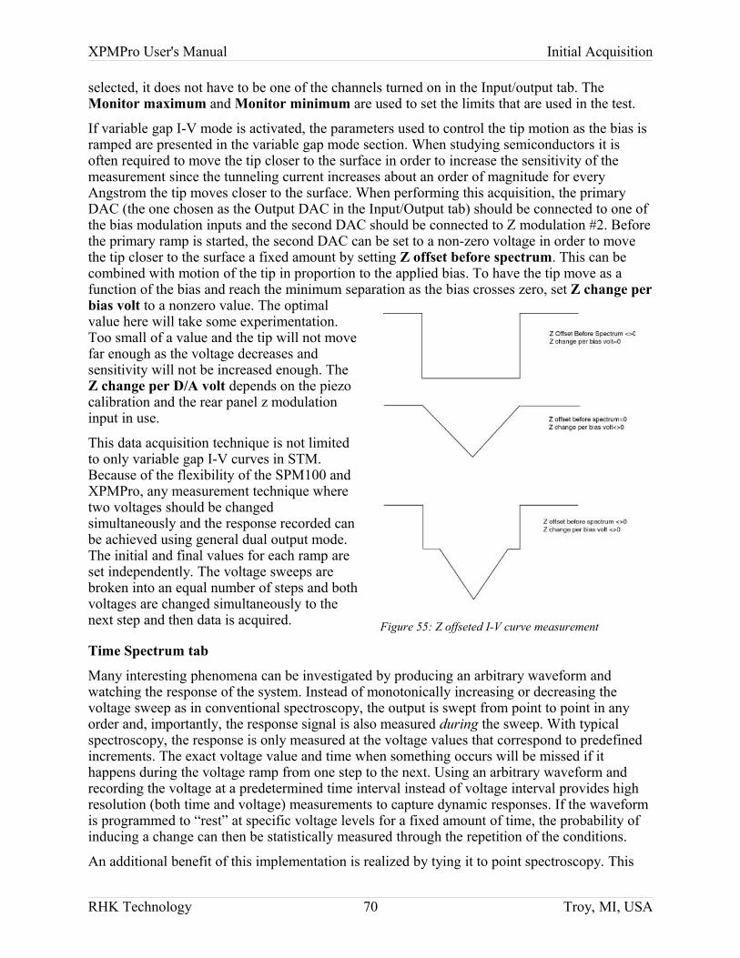
XPMPro User's Manual Initial Acquisition
selected, it does not have to be one of the channels turned on in the Input/output tab. The Monitor maximum and Monitor minimum are used to set the limits that are used in the test.
If variable gap I-V mode is activated, the parameters used to control the tip motion as the bias is ramped are presented in the variable gap mode section. When studying semiconductors it is often required to move the tip closer to the surface in order to increase the sensitivity of the measurement since the tunneling current increases about an order of magnitude for every Angstrom the tip moves closer to the surface. When performing this acquisition, the primary DAC (the one chosen as the Output DAC in the Input/Output tab) should be connected to one of the bias modulation inputs and the second DAC should be connected to Z modulation #2. Before the primary ramp is started, the second DAC can be set to a non-zero voltage in order to move the tip closer to the surface a fixed amount by setting Z offset before spectrum. This can be combined with motion of the tip in proportion to the applied bias. To have the tip move as a function of the bias and reach the minimum separation as the bias crosses zero, set Z change per bias volt to a nonzero value. The optimal value here will take some experimentation. Too small of a value and the tip will not move far enough as the voltage decreases and sensitivity will not be increased enough. The Z change per D/A volt depends on the piezo calibration and the rear panel z modulation input in use.
This data acquisition technique is not limited to only variable gap I-V curves in STM. Because of the flexibility of the SPM100 and XPMPro, any measurement technique where two voltages should be changed simultaneously and the response recorded can be achieved using general dual output mode. The initial and final values for each ramp are set independently. The voltage sweeps are broken into an equal number of steps and both voltages are changed simultaneously to the next step and then data is acquired.
Time Spectrum tab
Many interesting phenomena can be investigated by producing an arbitrary waveform and watching the response of the system. Instead of monotonically increasing or decreasing the voltage sweep as in conventional spectroscopy, the output is swept from point to point in any order and, importantly, the response signal is also measured during the sweep. With typical spectroscopy, the response is only measured at the voltage values that correspond to predefined increments. The exact voltage value and time when something occurs will be missed if it happens during the voltage ramp from one step to the next. Using an arbitrary waveform and recording the voltage at a predetermined time interval instead of voltage interval provides high resolution (both time and voltage) measurements to capture dynamic responses. If the waveform is programmed to “rest” at specific voltage levels for a fixed amount of time, the probability of inducing a change can then be statistically measured through the repetition of the conditions.
An additional benefit of this implementation is realized by tying it to point spectroscopy. This
RHK Technology 70 Troy, MI, USA
Figure 55: Z offseted I-V curve measurement
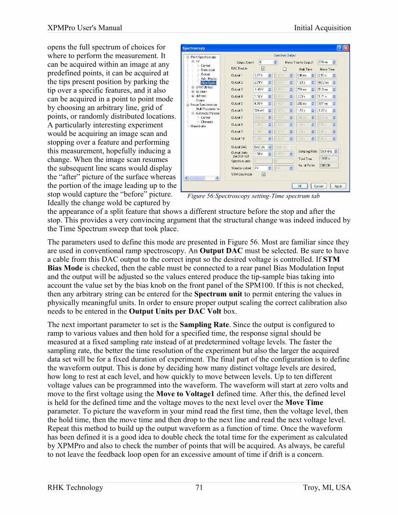
XPMPro User's Manual Initial Acquisition
opens the full spectrum of choices for where to perform the measurement. It can be acquired within an image at any predefined points, it can be acquired at the tips present position by parking the tip over a specific features, and it also can be acquired in a point to point mode by choosing an arbitrary line, grid of points, or randomly distributed locations. A particularly interesting experiment would be acquiring an image scan and stopping over a feature and performing this measurement, hopefully inducing a change. When the image scan resumes the subsequent line scans would display the “after” picture of the surface whereas the portion of the image leading up to the stop would capture the “before” picture. Ideally the change wold be captured by the appearance of a split feature that shows a different structure before the stop and after the stop. This provides a very convincing argument that the structural change was indeed induced by the Time Spectrum sweep that took place.
The parameters used to define this mode are presented in Figure 56. Most are familiar since they are used in conventional ramp spectroscopy. An Output DAC must be selected. Be sure to have a cable from this DAC output to the correct input so the desired voltage is controlled. If STM Bias Mode is checked, then the cable must be connected to a rear panel Bias Modulation Input and the output will be adjusted so the values entered produce the tip-sample bias taking into account the value set by the bias knob on the front panel of the SPM100. If this is not checked, then any arbitrary string can be entered for the Spectrum unit to permit entering the values in physically meaningful units. In order to ensure proper output scaling the correct calibration also needs to be entered in the Output Units per DAC Volt box.
The next important parameter to set is the Sampling Rate. Since the output is configured to ramp to various values and then hold for a specified time, the response signal should be measured at a fixed sampling rate instead of at predetermined voltage levels. The faster the sampling rate, the better the time resolution of the experiment but also the larger the acquired data set will be for a fixed duration of experiment. The final part of the configuration is to define the waveform output. This is done by deciding how many distinct voltage levels are desired, how long to rest at each level, and how quickly to move between levels. Up to ten different voltage values can be programmed into the waveform. The waveform will start at zero volts and move to the first voltage using the Move to Voltage1 defined time. After this, the defined level is held for the defined time and the voltage moves to the next level over the Move Time parameter. To picture the waveform in your mind read the first time, then the voltage level, then the hold time, then the move time and then drop to the next line and read the next voltage level. Repeat this method to build up the output waveform as a function of time. Once the waveform has been defined it is a good idea to double check the total time for the experiment as calculated by XPMPro and also to check the number of points that will be acquired. As always, be careful to not leave the feedback loop open for an excessive amount of time if drift is a concern.
RHK Technology 71 Troy, MI, USA
Figure 56:Spectroscopy setting-Time spectrum tab
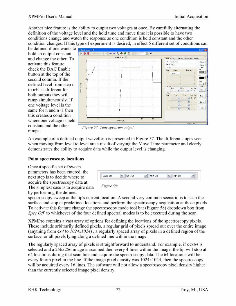
XPMPro User's Manual Initial Acquisition
Another nice feature is the ability to output two voltages at once. By carefully alternating the definition of the voltage level and the hold time and move time it is possible to have two conditions change and watch the response as one condition is held constant and the other condition changes. If this type of experiment is desired, in effect 5 different set of conditions can be defined if one wants to hold an output constant and change the other. To activate this feature, check the DAC Enable button at the top of the second column. If the defined level from step n to n+1 is different for both outputs they will ramp simultaneously. If one voltage level is the same for n and n+1 then this creates a condition where one voltage is held constant and the other ramps.
An example of a defined output waveform is presented in Figure 57. The different slopes seen when moving from level to level are a result of varying the Move Time parameter and clearly demonstrates the ability to acquire data while the output level is changing.
Point spectroscopy locations
Once a specific set of sweep parameters has been entered, the next step is to decide where to acquire the spectroscopy data at. The simplest case is to acquire data by performing the defined spectroscopy sweep at the tip's current location. A second very common scenario is to scan the surface and stop at predefined locations and perform the spectroscopy acquisition at those pixels. To activate this feature change the spectroscopy mode tool bar (Figure 58) dropdown box from Spec Off to whichever of the four defined spectral modes is to be executed during the scan.
XPMPro contains a vast array of options for defining the locations of the spectroscopy pixels. These include arbitrarily defined pixels, a regular grid of pixels spread out over the entire image (anything from 4x4 to 1024x1024) , a regularly spaced array of pixels in a defined region of the surface, or all pixels lying along a defined line within the image.
The regularly spaced array of pixels is straightforward to understand. For example, if 64x64 is selected and a 256x256 image is scanned then every 4 lines within the image, the tip will stop at 64 locations during that scan line and acquire the spectroscopy data. The 64 locations will be every fourth pixel in the line. If the image pixel density was 1024x1024, then the spectroscopy will be acquired every 16 lines. The software will not allow a spectroscopy pixel density higher than the currently selected image pixel density.
RHK Technology 72 Troy, MI, USA
Figure 58:
Figure 57: Time spectrum output
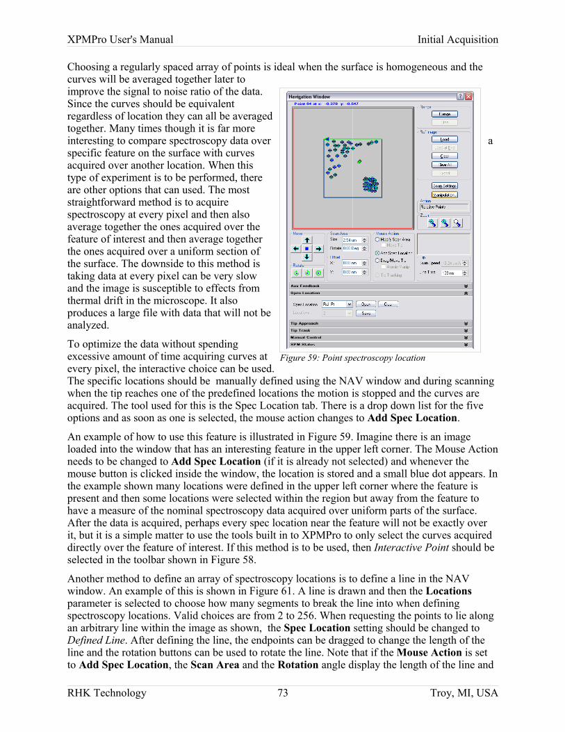
XPMPro User's Manual Initial Acquisition
Choosing a regularly spaced array of points is ideal when the surface is homogeneous and the curves will be averaged together later to improve the signal to noise ratio of the data. Since the curves should be equivalent regardless of location they can all be averaged together. Many times though it is far more interesting to compare spectroscopy data over a specific feature on the surface with curves acquired over another location. When this type of experiment is to be performed, there are other options that can used. The most straightforward method is to acquire spectroscopy at every pixel and then also average together the ones acquired over the feature of interest and then average together the ones acquired over a uniform section of the surface. The downside to this method is taking data at every pixel can be very slow and the image is susceptible to effects from thermal drift in the microscope. It also produces a large file with data that will not be analyzed.
To optimize the data without spending excessive amount of time acquiring curves at every pixel, the interactive choice can be used. The specific locations should be manually defined using the NAV window and during scanning when the tip reaches one of the predefined locations the motion is stopped and the curves are acquired. The tool used for this is the Spec Location tab. There is a drop down list for the five options and as soon as one is selected, the mouse action changes to Add Spec Location.
An example of how to use this feature is illustrated in Figure 59. Imagine there is an image loaded into the window that has an interesting feature in the upper left corner. The Mouse Action needs to be changed to Add Spec Location (if it is already not selected) and whenever the mouse button is clicked inside the window, the location is stored and a small blue dot appears. In the example shown many locations were defined in the upper left corner where the feature is present and then some locations were selected within the region but away from the feature to have a measure of the nominal spectroscopy data acquired over uniform parts of the surface. After the data is acquired, perhaps every spec location near the feature will not be exactly over it, but it is a simple matter to use the tools built in to XPMPro to only select the curves acquired directly over the feature of interest. If this method is to be used, then Interactive Point should be selected in the toolbar shown in Figure 58.
Another method to define an array of spectroscopy locations is to define a line in the NAV window. An example of this is shown in Figure 61. A line is drawn and then the Locations parameter is selected to choose how many segments to break the line into when defining spectroscopy locations. Valid choices are from 2 to 256. When requesting the points to lie along an arbitrary line within the image as shown, the Spec Location setting should be changed to Defined Line. After defining the line, the endpoints can be dragged to change the length of the line and the rotation buttons can be used to rotate the line. Note that if the Mouse Action is set to Add Spec Location, the Scan Area and the Rotation angle display the length of the line and
RHK Technology 73 Troy, MI, USA
Figure 59: Point spectroscopy location
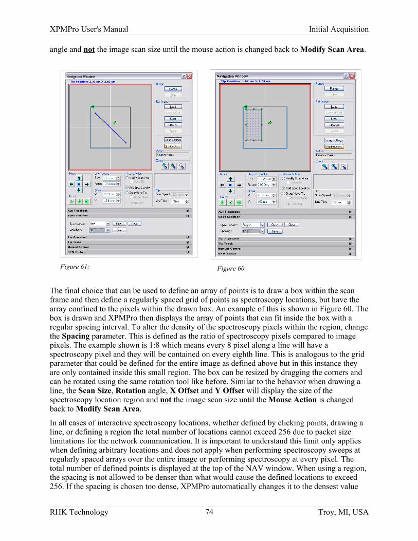
XPMPro User's Manual Initial Acquisition
angle and not the image scan size until the mouse action is changed back to Modify Scan Area.
The final choice that can be used to define an array of points is to draw a box within the scan frame and then define a regularly spaced grid of points as spectroscopy locations, but have the array confined to the pixels within the drawn box. An example of this is shown in Figure 60. The box is drawn and XPMPro then displays the array of points that can fit inside the box with a regular spacing interval. To alter the density of the spectroscopy pixels within the region, change the Spacing parameter. This is defined as the ratio of spectroscopy pixels compared to image pixels. The example shown is 1:8 which means every 8 pixel along a line will have a spectroscopy pixel and they will be contained on every eighth line. This is analogous to the grid parameter that could be defined for the entire image as defined above but in this instance they are only contained inside this small region. The box can be resized by dragging the corners and can be rotated using the same rotation tool like before. Similar to the behavior when drawing a line, the Scan Size, Rotation angle, X Offset and Y Offset will display the size of the spectroscopy location region and not the image scan size until the Mouse Action is changed back to Modify Scan Area.
In all cases of interactive spectroscopy locations, whether defined by clicking points, drawing a line, or defining a region the total number of locations cannot exceed 256 due to packet size limitations for the network communication. It is important to understand this limit only applies when defining arbitrary locations and does not apply when performing spectroscopy sweeps at regularly spaced arrays over the entire image or performing spectroscopy at every pixel. The total number of defined points is displayed at the top of the NAV window. When using a region, the spacing is not allowed to be denser than what would cause the defined locations to exceed 256. If the spacing is chosen too dense, XPMPro automatically changes it to the densest value
RHK Technology 74 Troy, MI, USA
Figure 61: Figure 60
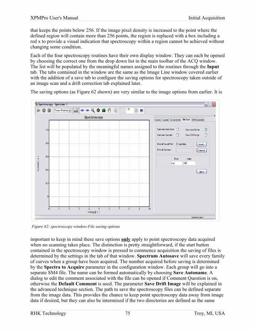
XPMPro User's Manual Initial Acquisition
that keeps the points below 256. If the image pixel density is increased to the point where the defined region will contain more than 256 points, the region is replaced with a box including a red x to provide a visual indication that spectroscopy within a region cannot be achieved without changing some condition.
Each of the four spectroscopy routines have their own display window. They can each be opened by choosing the correct one from the drop down list in the main toolbar of the ACQ window. The list will be populated by the meaningful names assigned to the routines through the Input tab. The tabs contained in the window are the same as the Image Line window covered earlier with the addition of a save tab to configure the saving options for spectroscopy taken outside of an image scan and a drift correction tab explained later.
The saving options (as Figure 62 shown) are very similar to the image options from earlier. It is
important to keep in mind these save options only apply to point spectroscopy data acquired when no scanning takes place. The distinction is pretty straightforward, if the start button contained in the spectroscopy window is pressed to commence acquisition the saving of files is determined by the settings in the tab of that window. Spectrum Autosave will save every family of curves when a group have been acquired. The number acquired before saving is determined by the Spectra to Acquire parameter in the configuration window. Each group will go into a separate SM4 file. The name can be formed automatically by choosing Save Autoname. A dialog to edit the comment associated with the file can be opened if Comment Question is on, otherwise the Default Comment is used. The parameter Save Drift Image will be explained in the advanced technique section. The path to save the spectroscopy files can be defined separate from the image data. This provides the chance to keep point spectroscopy data away from image data if desired, but they can also be intermixed if the two directories are defined as the same
RHK Technology 75 Troy, MI, USA
Figure 62: spectroscopy window-File saving options
XPMPro User's Manual Initial Acquisition
location. A separate comment can also be entered for spectroscopy data compared to the image data. If autonaming the files, the scheme used to form the name is determined by the root and index entered in this tab. This provides a nice facility to name spectroscopy files with a different name compared to image files. After any changes are made, be sure to click the Apply button so the changes take effect.
This window has some new controls and useful features related to spectroscopy. All of the graph windows in XPMPro have a common set of controls but also some buttons and tabs that are specific to the window. The first unique items noticed in this window are the start/stop buttons present in the main ACQ toolbar. If spectroscopy is to be acquired outside of an image scan, the controls to start and stop it are the ones in this window. As discussed above, there are four choices for the spectroscopy to be acquired. Use the dropdown list to choose what mode to perform when the acquisition is started. The four choices are Present Position, Relative Point, Defined Line, and Defined Region. The manner of defining these was discussed above and they serve the same purpose. The only difference between using the spectroscopy window to acquire the data and the image window is during this mode, the tip moves directly from point to point and only acquires spectroscopy data. It does not scan over a square region of the surface acquiring image data at pixel locations and also stop at these locations to acquire spectroscopy.
When multiple curves are present on the plot (Spectra to Acquire greater than 1) there is need to select an active curve both for highlighting and to place the cursors on a specific curve. This is done using the left and right arrow buttons. Each time one is clicked, the active curve increases or decreases by one. The active curve number is displayed in the gray box in the middle of the window. Additionally, when looking at stored data the status bar of the graph window will display the location of the tip when the highlighted curve was acquired. Next to the active curve selection buttons is a magnifying glass icon; this is used to zoom the plot. The mouse cursor changes shape when this is active. Click and drag to form a box that determines the new visible part of the curve. This method is usually more convenient than trying to manually adjust the x and y axis minimal and maximal to have only part of the curve visible. After zooming to the approximate region of interest, using the axis adjustment controls can be convenient for small adjustments. The next icon is for the cursors. There will be two placed on the plot and they can each be dragged around to take measurements from the plot. To see the values of the two locations, use the Cursor tab on the right side of the window. The final icon in the group that looks like a hand is used to pan the graph. The mouse cursor changes to a hand shape, click the mouse to “grab” the plot and drag it in any direction to shift the field of view a desired amount.
The next control is useful to handle plots that can have a large number of curves. If Spectra to Acquire is very large (hundreds or thousands) the plot may become confusing with so many lines drawn on it. The active entry box (32 in the figure) can be changed to determine the maximum number of plots displayed at one time. If this is smaller then the Spectra to Acquire value as a new curve is acquired, the oldest curve is dropped. Keep in mind the full set of curves will be saved in an SM4 file if the data is written to the hard drive, but they all do not have to be visible at once. This will be very beneficial in the DAW when analyzing data at a later time. If a measurement was taken that acquired tens of thousands of curves, it is not beneficial to try to look at them all at the same time because the plot will be too crowded. A reasonable number can be typed in this box so only a fixed number will be shown at any one time. For example, picking 1024 would mean the first 1024 of a file will be read and displayed. To browse another group, the double arrow buttons can be clicked. This loads the next group (1025 to 2048) or a previous group depending on which is clicked. The first box changes its value to reflect the curve number of the first one being displayed. The second number reflects the number of curves plotted in the graph.
RHK Technology 76 Troy, MI, USA
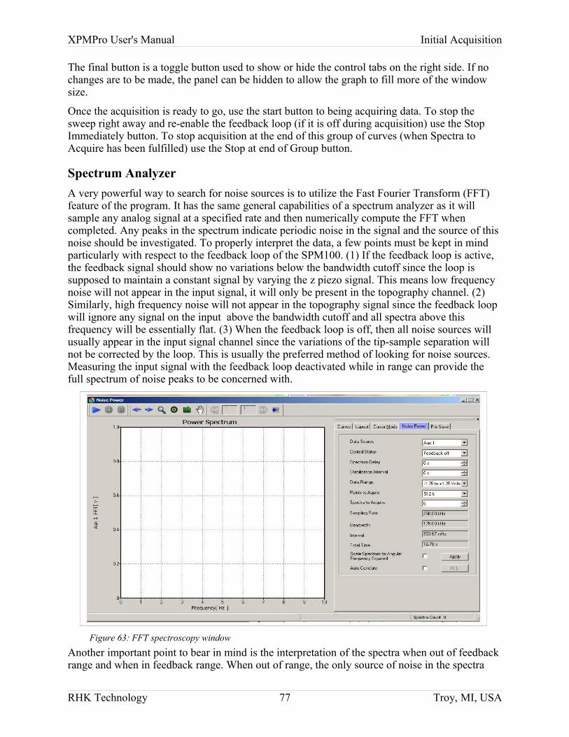
XPMPro User's Manual Initial Acquisition
The final button is a toggle button used to show or hide the control tabs on the right side. If no changes are to be made, the panel can be hidden to allow the graph to fill more of the window size.
Once the acquisition is ready to go, use the start button to being acquiring data. To stop the sweep right away and re-enable the feedback loop (if it is off during acquisition) use the Stop Immediately button. To stop acquisition at the end of this group of curves (when Spectra to Acquire has been fulfilled) use the Stop at end of Group button.
Spectrum AnalyzerA very powerful way to search for noise sources is to utilize the Fast Fourier Transform (FFT) feature of the program. It has the same general capabilities of a spectrum analyzer as it will sample any analog signal at a specified rate and then numerically compute the FFT when completed. Any peaks in the spectrum indicate periodic noise in the signal and the source of this noise should be investigated. To properly interpret the data, a few points must be kept in mind particularly with respect to the feedback loop of the SPM100. (1) If the feedback loop is active, the feedback signal should show no variations below the bandwidth cutoff since the loop is supposed to maintain a constant signal by varying the z piezo signal. This means low frequency noise will not appear in the input signal, it will only be present in the topography channel. (2) Similarly, high frequency noise will not appear in the topography signal since the feedback loop will ignore any signal on the input above the bandwidth cutoff and all spectra above this frequency will be essentially flat. (3) When the feedback loop is off, then all noise sources will usually appear in the input signal channel since the variations of the tip-sample separation will not be corrected by the loop. This is usually the preferred method of looking for noise sources. Measuring the input signal with the feedback loop deactivated while in range can provide the full spectrum of noise peaks to be concerned with.
Another important point to bear in mind is the interpretation of the spectra when out of feedback range and when in feedback range. When out of range, the only source of noise in the spectra
RHK Technology 77 Troy, MI, USA
Figure 63: FFT spectroscopy window
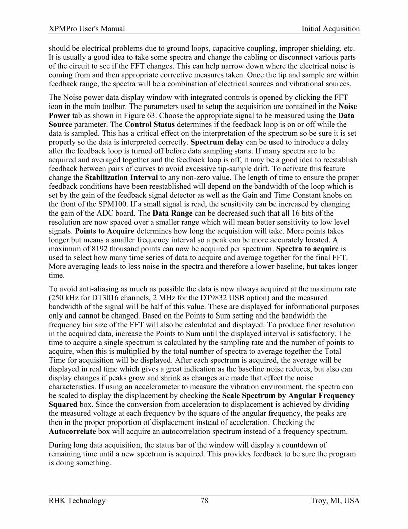
XPMPro User's Manual Initial Acquisition
should be electrical problems due to ground loops, capacitive coupling, improper shielding, etc. It is usually a good idea to take some spectra and change the cabling or disconnect various parts of the circuit to see if the FFT changes. This can help narrow down where the electrical noise is coming from and then appropriate corrective measures taken. Once the tip and sample are within feedback range, the spectra will be a combination of electrical sources and vibrational sources.
The Noise power data display window with integrated controls is opened by clicking the FFT icon in the main toolbar. The parameters used to setup the acquisition are contained in the Noise Power tab as shown in Figure 63. Choose the appropriate signal to be measured using the Data Source parameter. The Control Status determines if the feedback loop is on or off while the data is sampled. This has a critical effect on the interpretation of the spectrum so be sure it is set properly so the data is interpreted correctly. Spectrum delay can be used to introduce a delay after the feedback loop is turned off before data sampling starts. If many spectra are to be acquired and averaged together and the feedback loop is off, it may be a good idea to reestablish feedback between pairs of curves to avoid excessive tip-sample drift. To activate this feature change the Stabilization Interval to any non-zero value. The length of time to ensure the proper feedback conditions have been reestablished will depend on the bandwidth of the loop which is set by the gain of the feedback signal detector as well as the Gain and Time Constant knobs on the front of the SPM100. If a small signal is read, the sensitivity can be increased by changing the gain of the ADC board. The Data Range can be decreased such that all 16 bits of the resolution are now spaced over a smaller range which will mean better sensitivity to low level signals. Points to Acquire determines how long the acquisition will take. More points takes longer but means a smaller frequency interval so a peak can be more accurately located. A maximum of 8192 thousand points can now be acquired per spectrum. Spectra to acquire is used to select how many time series of data to acquire and average together for the final FFT. More averaging leads to less noise in the spectra and therefore a lower baseline, but takes longer time.
To avoid anti-aliasing as much as possible the data is now always acquired at the maximum rate (250 kHz for DT3016 channels, 2 MHz for the DT9832 USB option) and the measured bandwidth of the signal will be half of this value. These are displayed for informational purposes only and cannot be changed. Based on the Points to Sum setting and the bandwidth the frequency bin size of the FFT will also be calculated and displayed. To produce finer resolution in the acquired data, increase the Points to Sum until the displayed interval is satisfactory. The time to acquire a single spectrum is calculated by the sampling rate and the number of points to acquire, when this is multiplied by the total number of spectra to average together the Total Time for acquisition will be displayed. After each spectrum is acquired, the average will be displayed in real time which gives a great indication as the baseline noise reduces, but also can display changes if peaks grow and shrink as changes are made that effect the noise characteristics. If using an accelerometer to measure the vibration environment, the spectra can be scaled to display the displacement by checking the Scale Spectrum by Angular Frequency Squared box. Since the conversion from acceleration to displacement is achieved by dividing the measured voltage at each frequency by the square of the angular frequency, the peaks are then in the proper proportion of displacement instead of acceleration. Checking the Autocorrelate box will acquire an autocorrelation spectrum instead of a frequency spectrum.
During long data acquisition, the status bar of the window will display a countdown of remaining time until a new spectrum is acquired. This provides feedback to be sure the program is doing something.
RHK Technology 78 Troy, MI, USA
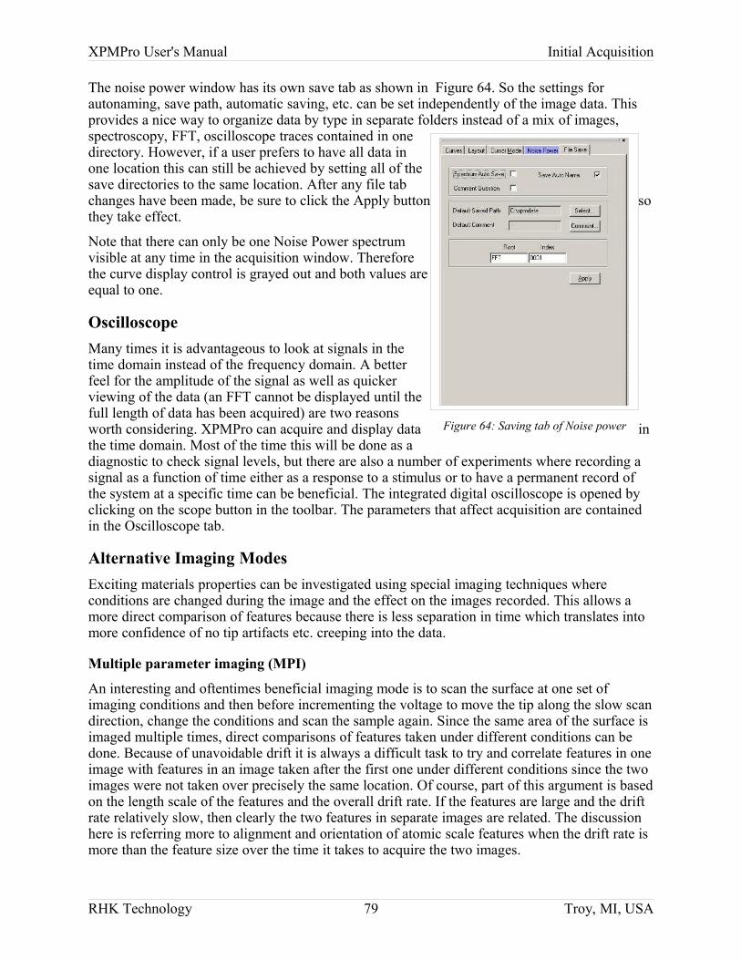
XPMPro User's Manual Initial Acquisition
The noise power window has its own save tab as shown in Figure 64. So the settings for autonaming, save path, automatic saving, etc. can be set independently of the image data. This provides a nice way to organize data by type in separate folders instead of a mix of images, spectroscopy, FFT, oscilloscope traces contained in one directory. However, if a user prefers to have all data in one location this can still be achieved by setting all of the save directories to the same location. After any file tab changes have been made, be sure to click the Apply button so they take effect.
Note that there can only be one Noise Power spectrum visible at any time in the acquisition window. Therefore the curve display control is grayed out and both values are equal to one.
Oscilloscope Many times it is advantageous to look at signals in the time domain instead of the frequency domain. A better feel for the amplitude of the signal as well as quicker viewing of the data (an FFT cannot be displayed until the full length of data has been acquired) are two reasons worth considering. XPMPro can acquire and display data in the time domain. Most of the time this will be done as a diagnostic to check signal levels, but there are also a number of experiments where recording a signal as a function of time either as a response to a stimulus or to have a permanent record of the system at a specific time can be beneficial. The integrated digital oscilloscope is opened by clicking on the scope button in the toolbar. The parameters that affect acquisition are contained in the Oscilloscope tab.
Alternative Imaging ModesExciting materials properties can be investigated using special imaging techniques where conditions are changed during the image and the effect on the images recorded. This allows a more direct comparison of features because there is less separation in time which translates into more confidence of no tip artifacts etc. creeping into the data.
Multiple parameter imaging (MPI)
An interesting and oftentimes beneficial imaging mode is to scan the surface at one set of imaging conditions and then before incrementing the voltage to move the tip along the slow scan direction, change the conditions and scan the sample again. Since the same area of the surface is imaged multiple times, direct comparisons of features taken under different conditions can be done. Because of unavoidable drift it is always a difficult task to try and correlate features in one image with features in an image taken after the first one under different conditions since the two images were not taken over precisely the same location. Of course, part of this argument is based on the length scale of the features and the overall drift rate. If the features are large and the drift rate relatively slow, then clearly the two features in separate images are related. The discussion here is referring more to alignment and orientation of atomic scale features when the drift rate is more than the feature size over the time it takes to acquire the two images.
RHK Technology 79 Troy, MI, USA
Figure 64: Saving tab of Noise power
XPMPro User's Manual Initial Acquisition
XPMPro allows the same area of the surface to be scanned up to four times under different conditions. In this imaging mode, eight individual images would be acquired (four sets of conditions, 2 scan directions) and stored in a single file. The tab to configure this mode is contained in the Settings/Spectroscopy window and is named Multi as shown in Figure 65. To activate this data acquisition routine during scanning, the Multi Volt toolbar box (Figure 58) should be changed from MPI Off to the desired mode. The two most common choices would be either multi page or dynamic lithography; in both cases the same section of the surface is scanned repeated times as described above. In an unusual mode, split page mode, the scan proceeds with a normal slow raster, but partway through the image, the conditions are changed so the lower section of the image is not acquired under the same conditions as the top part.
The channels recorded during rescan are the same ones recorded during the first scan, which are all channels turned on in the Settings/Scan/Input tab.
The first parameter sets the number of times to scan over the same line before incrementing along the slow scan direction. This can be set to either 2, 3, or 4. It does not make sense to set this parameter to one since this would be the same as conventional imaging. At the end of the reverse line-scan the conditions are changed and before the next line is started, the SPM100 pauses for a length of time specified by the Voltage change delay. This is usually necessary in order for the feedback loop to adjust to the new imaging conditions. The amount of time will be dependent on the bandwidth of the feedback loop. The next four parameters are the voltage levels to output for each scan over the surface. The first voltage is usually set to zero when not doing STM or set to the nominal bias voltage determined by the SPM100 knob when performing STM. Note the nominal imaging conditions are not used for any of the scans unless specifically configured to do so. The feedback loop can also be disabled during the subsequent rescans if desired. If performing conventional imaging of recording the channels under various conditions, the loop would remain on during these rescans. If an advanced mode such as dynamic lithography is performed, then the loop may need to be disabled during the rescans.
When multi-volt imaging is turned off, the output is set to the Standby voltage which in almost all cases should be zero. Otherwise, the conventional imaging acquired after the mode has been turned off will not be the same as before because the additional voltage applied will effect the imaging conditions in some manner and may be unaccounted for when interpreting the images later. If the four voltages specified are meant to change the tunneling bias during STM, then
RHK Technology 80 Troy, MI, USA
Figure 65: Multi Parameter Image setting
XPMPro User's Manual Initial Acquisition
STM Bias Mode should be on. The actual DAC output will be adjusted such that the sum of it and the bias knob setting is equal to the requested value If the parameter is off, then the DAC output will be exactly equal to the value entered in the window. If zero is entered for one of the voltage values and STM Bias Mode is on, the DAC will counteract the bias knob resulting in a tunneling bias of zero which will cause a tip crash!
If the output voltage is affecting some other physical quantity, then the Output units can be entered here so the values are entered, displayed, and stored in the meaningful unit instead of volts. The conversion of the DAC output into the meaningful quantity is entered in the parameter named Output units per D/A volt. Whenever the voltage is changed from one value to the next, enter a speed that it should be changed using the Ramp speed parameter. This can be used to reduce or even eliminate transients that could be induced in the system by a sudden change in voltage level. The Output DAC is the channel that should produce the voltage. A BNC cable must be connected from this channel to the appropriate input for the desired change in imaging conditions to occur.
Dynamic lithography has many uses for new and exciting data acquisition and should be carefully considered. The implementation allows a signal to be recorded by the DSP board and as it rescans the same line over, it can output the data recorded at the corresponding pixel during the initial trip across the surface. Additionally, with a future implementation the user will have the opportunity to download a shape into the DSP board and have it output this as the tip scans. As long as the number of points in the shape equals the number of pixels in the line scan, the system will work. By recording a signal (such as topography or other channel) during the first scan, the replay is assured of having the equal number of pixels as the rescan line.
The line can then be rescanned up to three more times with conditions changed to acquire a set of images at the same time that show the topography and other signals acquired over the same area of the surface to permit correlation. The changed voltage can be applied to any input (internal or external) to achieve any desired result. It could change a magnetic field, the tunneling bias, temperature, a z piezo to pull the tip off the surface or push the tip into the surface, or a lockin amplifier to apply an oscillation to some signal. The loop can also be disabled; in the case of applying the replay voltage to a z piezo this would be required. Otherwise the loop would simply counteract the applied voltage and not change the relative tip height above the sample.
Since the only mode currently available is to record a signal and play it back on rescans, the correct cabling is imperative to properly interpret the result. Whatever signal is to be recorded should be connected to DSP ADC#1 on the SPM100 rear panel. The output signal on scans 2, 3, and 4 will appear on DSP DAC. An additional connector is also require so the DSP board properly records the signal. The rear panel Digital IO connector needs to have pins 3 and 6 shorted together. The simplest method to achieve this is to obtain a mating connector and solder a single wire between the two pins and then attach it to the rear panel.
If the output is to be scaled from the recorded signal, use the Output Multiplier parameter. An example of this is when the Z Position monitor output is connected to ADC #1 to record topography. Since this output has the front panel ADC gain applied, the recorded voltage is larger than the actual variations. To reduce the voltage applied to the z piezo when the DSP DAC is connected to Z Position #1 modulation input to properly replay the topographic variations, the inverse of the ADC gain will be automatically corrected when Z monitor is selected as the output mode. If the Z monitor is selected to be the output mode, the front panel ADC gain knob is not allowed to adjust when the tip is scanning. Otherwise, the tip
RHK Technology 81 Troy, MI, USA
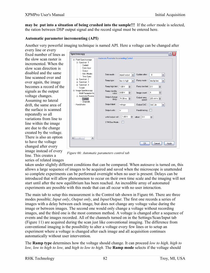
XPMPro User's Manual Initial Acquisition
may be put into a situation of being crashed into the sample!!! If the other mode is selected, the ration between DSP output signal and the record signal must be entered here.
Automatic parameter incrementing (API)
Another very powerful imaging technique is named API. Here a voltage can be changed after every line or every fixed number of lines as the slow scan raster is incremented. When the slow scan direction is disabled and the same line scanned over and over again, the image becomes a record of the signals as the output voltage changes. Assuming no lateral drift, the same area of the surface is scanned repeatedly so all variations from line to line within the image are due to the change created by the voltage. There is also an option to have the voltage changed after every image instead of every line. This creates a series of related images taken under slightly different conditions that can be compared. When autosave is turned on, this allows a large sequence of images to be acquired and saved when the microscope is unattended so complete experiments can be performed overnight when no user is present. Delays can be introduced that will allow phenomenon to occur on their own time scale and the imaging will not start until after the new equilibrium has been reached. An incredible array of automated experiments are possible with this mode that can all occur with no user interaction.
The main tab to setup this measurement is the Control tab shown in Figure 66. There are three modes possible; Input only, Output only, and Input/Output. The first one records a series of images with a delay between each image, but does not change any voltage value during the image or between images. The second one would only change a voltage without recording images, and the third one is the most common method. A voltage is changed after a sequence of events and the images recorded. All of the channels turned on in the Settings/Scan/Input tab (Figure 11) are acquired during the scan just like conventional imaging. The difference from conventional imaging is the possibility to alter a voltage every few lines or to setup an experiment where a voltage is changed after each image and all acquisition continues automatically without user intervention.
The Ramp type determines how the voltage should change. It can proceed low to high, high to low, low to high to low, and high to low to high. The Ramp mode selects if the voltage should
RHK Technology 82 Troy, MI, USA
Figure 66: Automatic parameters control tab
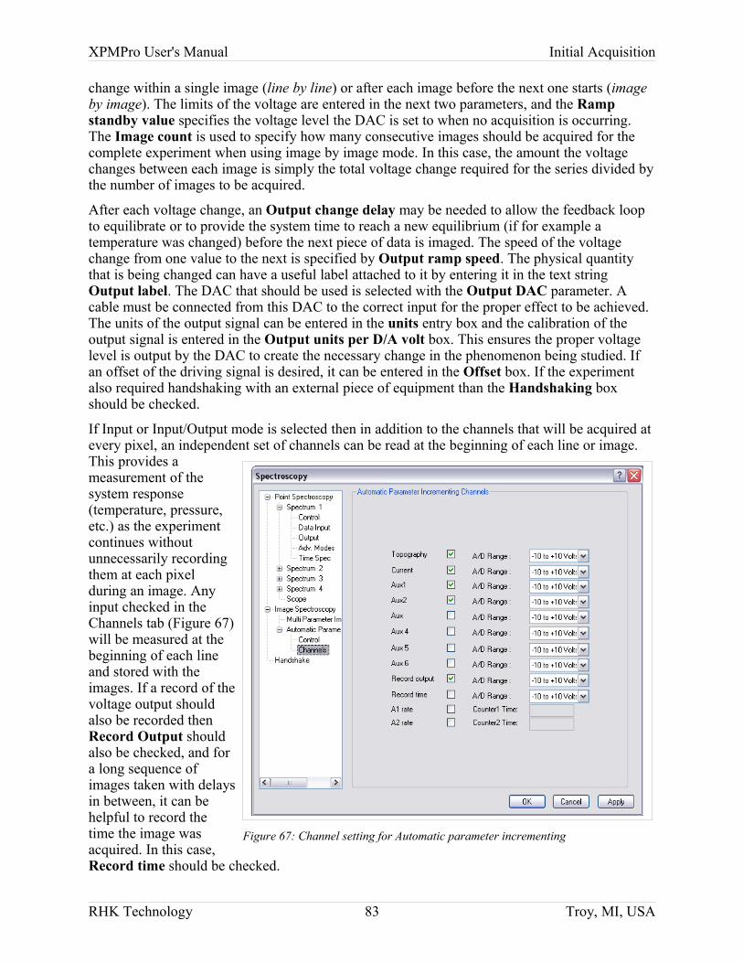
XPMPro User's Manual Initial Acquisition
change within a single image (line by line) or after each image before the next one starts (image by image). The limits of the voltage are entered in the next two parameters, and the Ramp standby value specifies the voltage level the DAC is set to when no acquisition is occurring. The Image count is used to specify how many consecutive images should be acquired for the complete experiment when using image by image mode. In this case, the amount the voltage changes between each image is simply the total voltage change required for the series divided by the number of images to be acquired.
After each voltage change, an Output change delay may be needed to allow the feedback loop to equilibrate or to provide the system time to reach a new equilibrium (if for example a temperature was changed) before the next piece of data is imaged. The speed of the voltage change from one value to the next is specified by Output ramp speed. The physical quantity that is being changed can have a useful label attached to it by entering it in the text string Output label. The DAC that should be used is selected with the Output DAC parameter. A cable must be connected from this DAC to the correct input for the proper effect to be achieved. The units of the output signal can be entered in the units entry box and the calibration of the output signal is entered in the Output units per D/A volt box. This ensures the proper voltage level is output by the DAC to create the necessary change in the phenomenon being studied. If an offset of the driving signal is desired, it can be entered in the Offset box. If the experiment also required handshaking with an external piece of equipment than the Handshaking box should be checked.
If Input or Input/Output mode is selected then in addition to the channels that will be acquired at every pixel, an independent set of channels can be read at the beginning of each line or image. This provides a measurement of the system response (temperature, pressure, etc.) as the experiment continues without unnecessarily recording them at each pixel during an image. Any input checked in the Channels tab (Figure 67) will be measured at the beginning of each line and stored with the images. If a record of the voltage output should also be recorded then Record Output should also be checked, and for a long sequence of images taken with delays in between, it can be helpful to record the time the image was acquired. In this case, Record time should be checked.
RHK Technology 83 Troy, MI, USA
Figure 67: Channel setting for Automatic parameter incrementing
XPMPro User's Manual Data Analysis and Image Processing
Analysis and Processing
RHK Technology 84 Troy, MI, USA
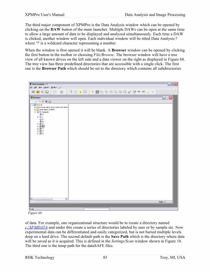
XPMPro User's Manual Data Analysis and Image Processing
The third major component of XPMPro is the Data Analysis window which can be opened by clicking on the DAW button of the main launcher. Multiple DAWs can be open at the same time to allow a large amount of data to be displayed and analyzed simultaneously. Each time a DAW is clicked, another window will open. Each individual window will be titled Data Analysis:? where '?' is a wildcard character representing a number.
When the window is first opened it will be blank. A Browser window can be opened by clicking the first button in the toolbar or choosing File/Browse. The browser window will have a tree view of all known drives on the left side and a data viewer on the right as displayed in Figure 68. The tree view has three predefined directories that are accessible with a single click. The first one is the Browser Path which should be set to the directory which contains all subdirectories
of data. For example, one organizational structure would be to create a directory named c:\SPMDATA and under this create a series of directories labeled by user or by sample etc. Now experimental data can be differentiated and easily categorized, but is not buried multiple levels deep on a hard drive. The second default path is the Save Path which is the directory where data will be saved as it is acquired. This is defined in the Settings/Scan window shown in Figure 10. The third one is the temp path for the dataSAFE files.
RHK Technology 85 Troy, MI, USA
Figure 68
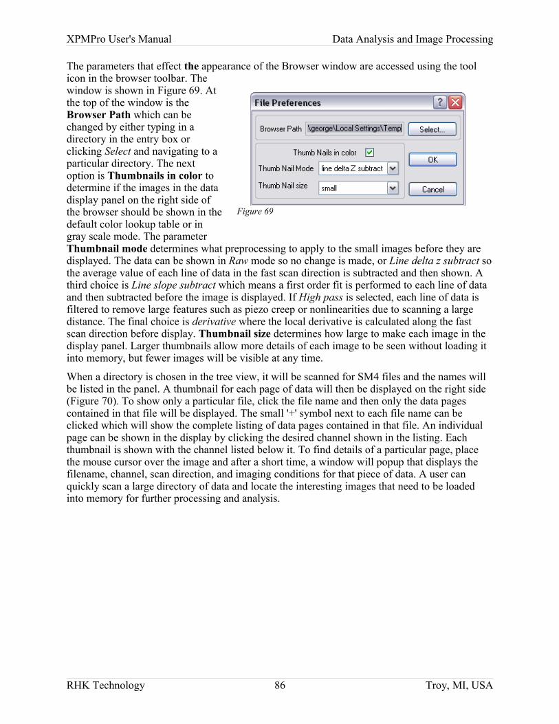
XPMPro User's Manual Data Analysis and Image Processing
The parameters that effect the appearance of the Browser window are accessed using the tool icon in the browser toolbar. The window is shown in Figure 69. At the top of the window is the Browser Path which can be changed by either typing in a directory in the entry box or clicking Select and navigating to a particular directory. The next option is Thumbnails in color to determine if the images in the data display panel on the right side of the browser should be shown in the default color lookup table or in gray scale mode. The parameter Thumbnail mode determines what preprocessing to apply to the small images before they are displayed. The data can be shown in Raw mode so no change is made, or Line delta z subtract so the average value of each line of data in the fast scan direction is subtracted and then shown. A third choice is Line slope subtract which means a first order fit is performed to each line of data and then subtracted before the image is displayed. If High pass is selected, each line of data is filtered to remove large features such as piezo creep or nonlinearities due to scanning a large distance. The final choice is derivative where the local derivative is calculated along the fast scan direction before display. Thumbnail size determines how large to make each image in the display panel. Larger thumbnails allow more details of each image to be seen without loading it into memory, but fewer images will be visible at any time.
When a directory is chosen in the tree view, it will be scanned for SM4 files and the names will be listed in the panel. A thumbnail for each page of data will then be displayed on the right side (Figure 70). To show only a particular file, click the file name and then only the data pages contained in that file will be displayed. The small '+' symbol next to each file name can be clicked which will show the complete listing of data pages contained in that file. An individual page can be shown in the display by clicking the desired channel shown in the listing. Each thumbnail is shown with the channel listed below it. To find details of a particular page, place the mouse cursor over the image and after a short time, a window will popup that displays the filename, channel, scan direction, and imaging conditions for that piece of data. A user can quickly scan a large directory of data and locate the interesting images that need to be loaded into memory for further processing and analysis.
RHK Technology 86 Troy, MI, USA
Figure 69
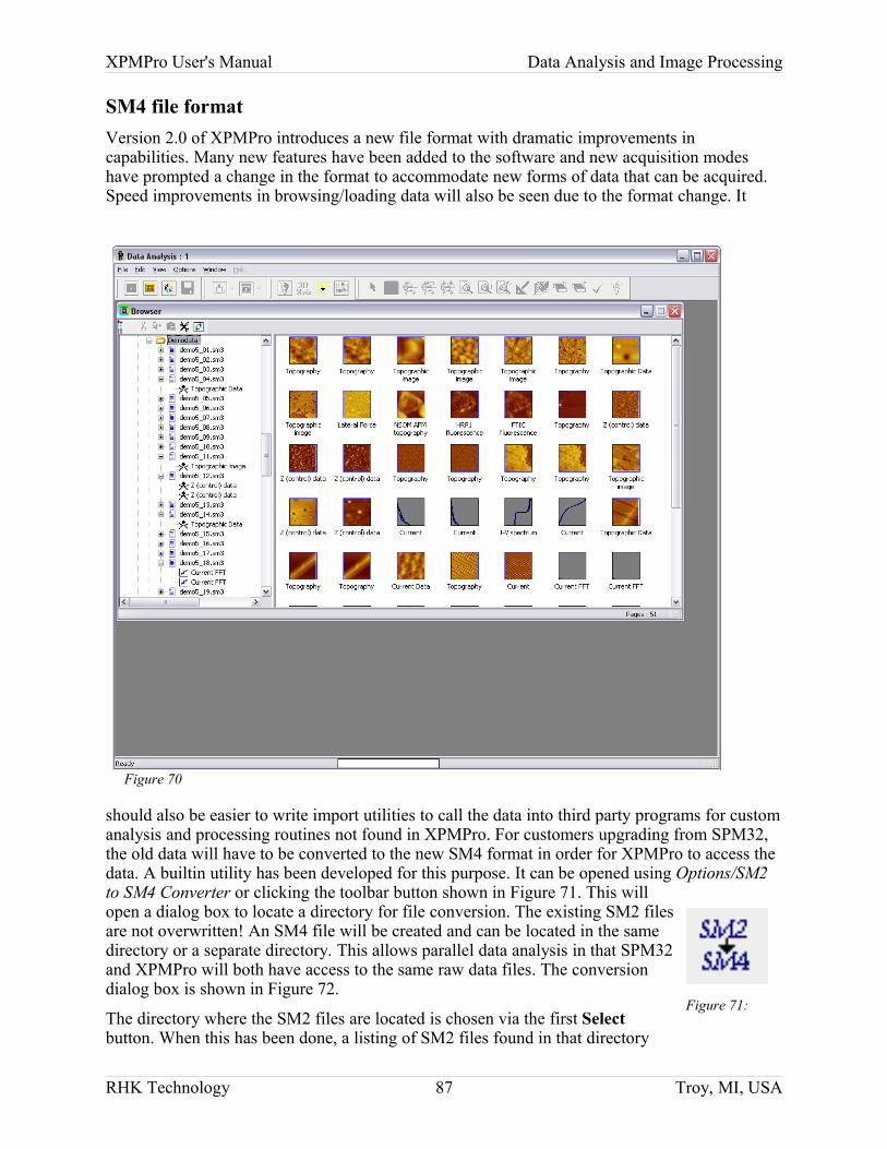
XPMPro User's Manual Data Analysis and Image Processing
SM4 file formatVersion 2.0 of XPMPro introduces a new file format with dramatic improvements in capabilities. Many new features have been added to the software and new acquisition modes have prompted a change in the format to accommodate new forms of data that can be acquired. Speed improvements in browsing/loading data will also be seen due to the format change. It
should also be easier to write import utilities to call the data into third party programs for custom analysis and processing routines not found in XPMPro. For customers upgrading from SPM32, the old data will have to be converted to the new SM4 format in order for XPMPro to access the data. A builtin utility has been developed for this purpose. It can be opened using Options/SM2 to SM4 Converter or clicking the toolbar button shown in Figure 71. This will open a dialog box to locate a directory for file conversion. The existing SM2 files are not overwritten! An SM4 file will be created and can be located in the same directory or a separate directory. This allows parallel data analysis in that SPM32 and XPMPro will both have access to the same raw data files. The conversion dialog box is shown in Figure 72.
The directory where the SM2 files are located is chosen via the first Select button. When this has been done, a listing of SM2 files found in that directory
RHK Technology 87 Troy, MI, USA
Figure 70
Figure 71:
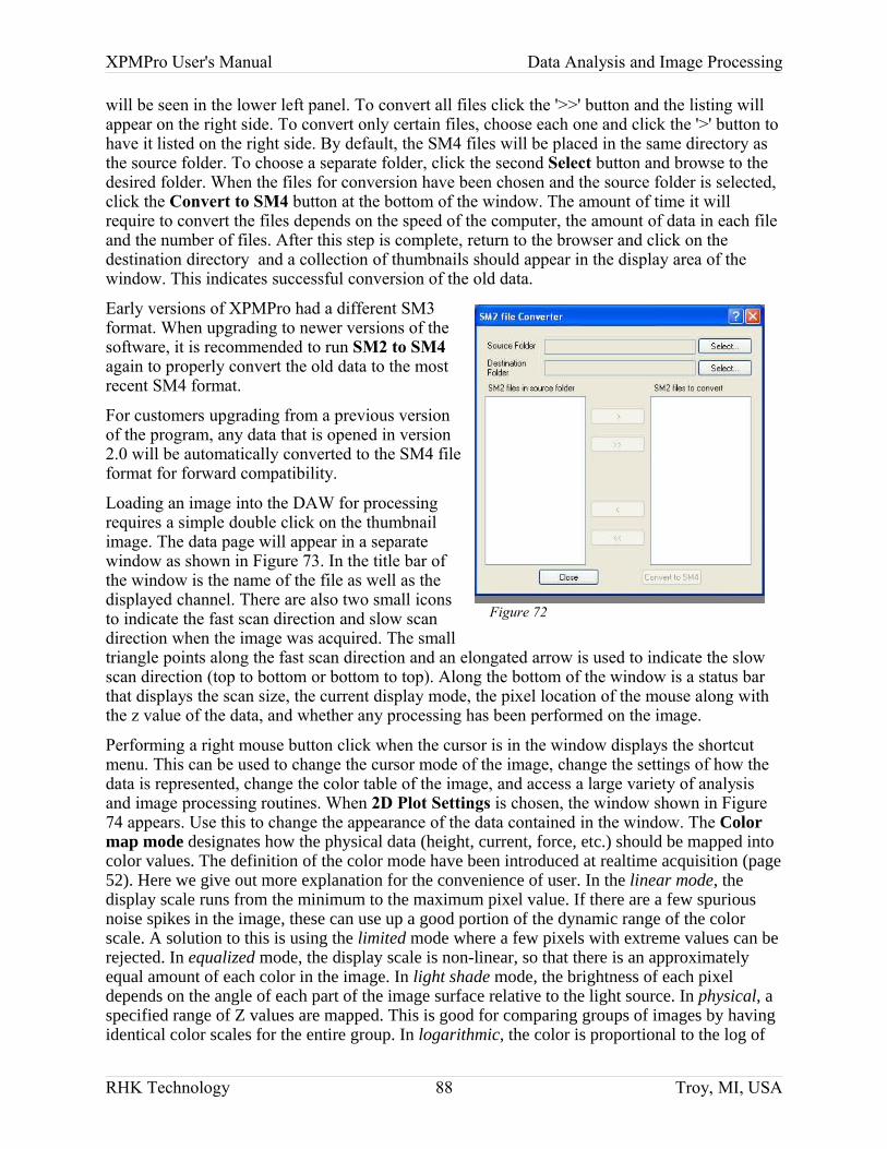
XPMPro User's Manual Data Analysis and Image Processing
will be seen in the lower left panel. To convert all files click the '>>' button and the listing will appear on the right side. To convert only certain files, choose each one and click the '>' button to have it listed on the right side. By default, the SM4 files will be placed in the same directory as the source folder. To choose a separate folder, click the second Select button and browse to the desired folder. When the files for conversion have been chosen and the source folder is selected, click the Convert to SM4 button at the bottom of the window. The amount of time it will require to convert the files depends on the speed of the computer, the amount of data in each file and the number of files. After this step is complete, return to the browser and click on the destination directory and a collection of thumbnails should appear in the display area of the window. This indicates successful conversion of the old data.
Early versions of XPMPro had a different SM3 format. When upgrading to newer versions of the software, it is recommended to run SM2 to SM4 again to properly convert the old data to the most recent SM4 format.
For customers upgrading from a previous version of the program, any data that is opened in version 2.0 will be automatically converted to the SM4 file format for forward compatibility.
Loading an image into the DAW for processing requires a simple double click on the thumbnail image. The data page will appear in a separate window as shown in Figure 73. In the title bar of the window is the name of the file as well as the displayed channel. There are also two small icons to indicate the fast scan direction and slow scan direction when the image was acquired. The small triangle points along the fast scan direction and an elongated arrow is used to indicate the slow scan direction (top to bottom or bottom to top). Along the bottom of the window is a status bar that displays the scan size, the current display mode, the pixel location of the mouse along with the z value of the data, and whether any processing has been performed on the image.
Performing a right mouse button click when the cursor is in the window displays the shortcut menu. This can be used to change the cursor mode of the image, change the settings of how the data is represented, change the color table of the image, and access a large variety of analysis and image processing routines. When 2D Plot Settings is chosen, the window shown in Figure74 appears. Use this to change the appearance of the data contained in the window. The Color map mode designates how the physical data (height, current, force, etc.) should be mapped into color values. The definition of the color mode have been introduced at realtime acquisition (page 52). Here we give out more explanation for the convenience of user. In the linear mode, the display scale runs from the minimum to the maximum pixel value. If there are a few spurious noise spikes in the image, these can use up a good portion of the dynamic range of the color scale. A solution to this is using the limited mode where a few pixels with extreme values can be rejected. In equalized mode, the display scale is non-linear, so that there is an approximately equal amount of each color in the image. In light shade mode, the brightness of each pixel depends on the angle of each part of the image surface relative to the light source. In physical, a specified range of Z values are mapped. This is good for comparing groups of images by having identical color scales for the entire group. In logarithmic, the color is proportional to the log of
RHK Technology 88 Troy, MI, USA
Figure 72
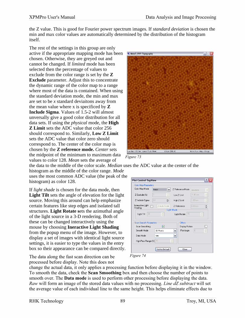
XPMPro User's Manual Data Analysis and Image Processing
the Z value. This is good for Fourier power spectrum images. If standard deviation is chosen the min and max color values are automatically determined by the distribution of the histogram itself.
The rest of the settings in this group are only active if the appropriate mapping mode has been chosen. Otherwise, they are greyed out and cannot be changed. If limited mode has been selected then the percentage of values to exclude from the color range is set by the Z Exclude parameter. Adjust this to concentrate the dynamic range of the color map to a range where most of the data is contained. When using the standard deviation mode, the min and max are set to be x standard deviaitons away from the mean value where x is specificed by Z Include Sigma. Values of 1.5-2 will almost unversally give a good color distribution for all data sets. If using the physical mode, the High Z Limit sets the ADC value that color 256 should correspond to. Similarly, Low Z Limit sets the ADC value that color zero should correspond to. The center of the color map is chosen by the Z reference mode. Center sets the midpoint of the minimum to maximum data values to color 128. Mean sets the average of the data to the middle of the color scale. Median uses the ADC value at the center of the histogram as the middle of the color range. Mode uses the most common ADC value (the peak of the histogram) as color 128.
If light shade is chosen for the data mode, then Light Tilt sets the angle of elevation for the light source. Moving this around can help emphasize certain features like step edges and isolated tall structures. Light Rotate sets the azimuthal angle of the light source in a 3-D rendering. Both of these can be changed interactively using the mouse by choosing Ineractive Light Shading from the popup menu of the image. However, to display a set of images with identical light source settings, it is easier to type the values in the entry box so their appearance can be compared directly.
The data along the fast scan direction can be processed before display. Note this does not change the actual data, it only applies a processing function before displaying it in the window. To smooth the data, check the Scan Smoothing box and then choose the number of points to smooth over. The Data mode is used to perform other processing before displaying the data. Raw will form an image of the stored data values with no processing. Line dZ subtract will set the average value of each individual line to the same height. This helps eliminate effects due to
RHK Technology 89 Troy, MI, USA
Figure 74
Figure 73
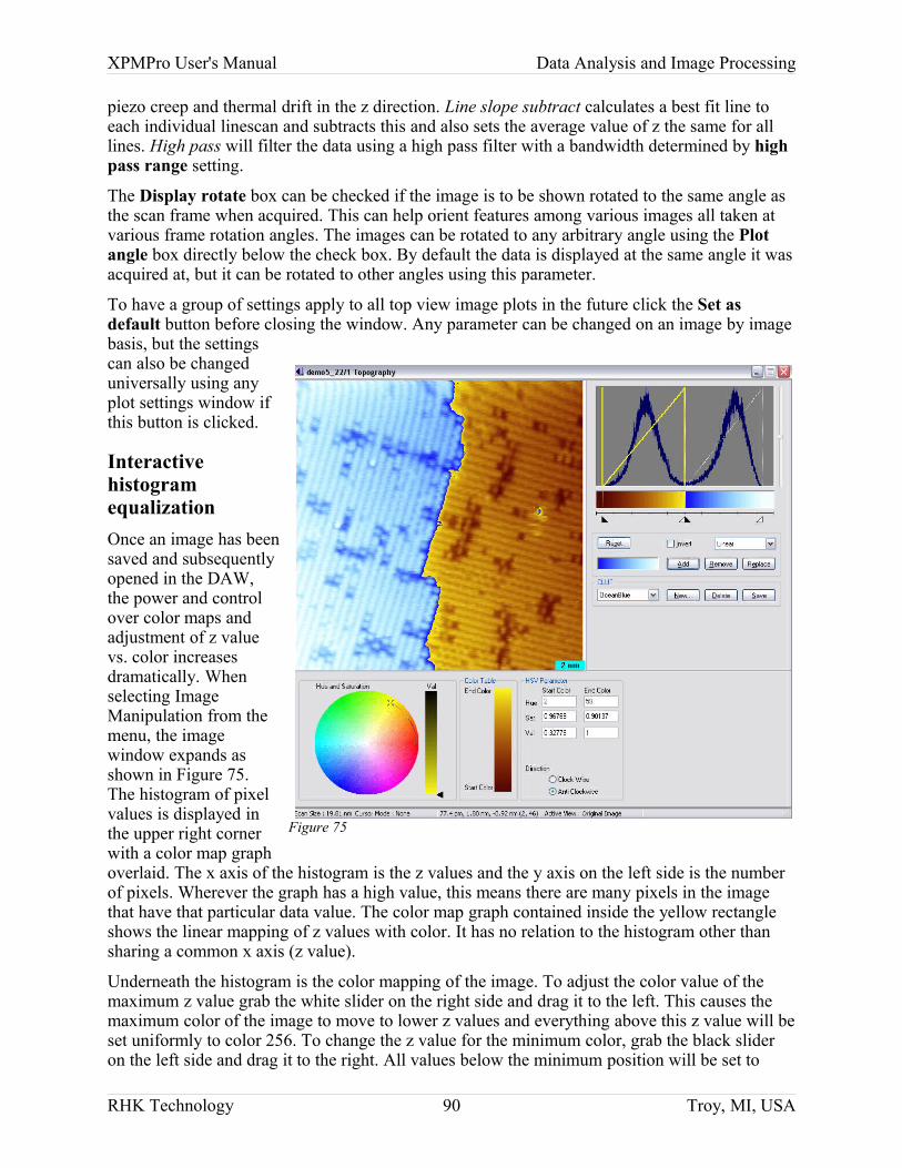
XPMPro User's Manual Data Analysis and Image Processing
piezo creep and thermal drift in the z direction. Line slope subtract calculates a best fit line to each individual linescan and subtracts this and also sets the average value of z the same for all lines. High pass will filter the data using a high pass filter with a bandwidth determined by high pass range setting.
The Display rotate box can be checked if the image is to be shown rotated to the same angle as the scan frame when acquired. This can help orient features among various images all taken at various frame rotation angles. The images can be rotated to any arbitrary angle using the Plot angle box directly below the check box. By default the data is displayed at the same angle it was acquired at, but it can be rotated to other angles using this parameter.
To have a group of settings apply to all top view image plots in the future click the Set as default button before closing the window. Any parameter can be changed on an image by image basis, but the settings can also be changed universally using any plot settings window if this button is clicked.
Interactive histogram equalizationOnce an image has been saved and subsequently opened in the DAW, the power and control over color maps and adjustment of z value vs. color increases dramatically. When selecting Image Manipulation from the menu, the image window expands as shown in Figure 75. The histogram of pixel values is displayed in the upper right corner with a color map graph overlaid. The x axis of the histogram is the z values and the y axis on the left side is the number of pixels. Wherever the graph has a high value, this means there are many pixels in the image that have that particular data value. The color map graph contained inside the yellow rectangle shows the linear mapping of z values with color. It has no relation to the histogram other than sharing a common x axis (z value).
Underneath the histogram is the color mapping of the image. To adjust the color value of the maximum z value grab the white slider on the right side and drag it to the left. This causes the maximum color of the image to move to lower z values and everything above this z value will be set uniformly to color 256. To change the z value for the minimum color, grab the black slider on the left side and drag it to the right. All values below the minimum position will be set to
RHK Technology 90 Troy, MI, USA
Figure 75

XPMPro User's Manual Data Analysis and Image Processing
color zero of the current CLUT.
Once there are gaps in the color mapping, additional color scales can be added. These can be done for artistic purposes or to help emphasize certain features in the image that may be easier to notice with sharper contrast between z values. To add a new color scale, choose alone from the CLUT drop down box and then click the Add button. Move the cursor up to the color scale region of the histogram graph and when its appearance changes to a '+' symbol, it can be clicked and the new color scale fills in this gap. After adding it, a new set of sliders will be added to the x axis region and the mapping of this CLUT to z values can be changed by dragging them. To remove a color scale, first click the mouse cursor in the region that contains the one to remove which turns that overlaid graph yellow to indicate it is the active one. Once this is done click the Delete button. The CLUT disappears and all z values previously mapped to it return to the value determined by the remaining sets of sliders.
To edit the active CLUT, use the color wheel in the lower corner in the same manner as described previously. Move the start color and end color endpoints of the line. The image appearance will change as the endpoints are dragged to provide immediate visual feedback of the changes. Color lookup tables can be changed, created or deleted from this window similar to the functions presented in the color wheel dialog from the realtime acquisition windows.
To change the color mapping from a simple linear mode to non-linear graphs, select the correction mode from the dropdown just below the color scale. The three choices are Linear, Gamma, and Double Gamma. Once the mode is changed to one of the gamma selections, the overlaid graph is changed by using the vertical slider on the right side of the histogram graph. Keep in mind the axes for the graph can be thought of as z values along the x axis and color 0 to color 256 along the y axis.
When all of the changes are satisfactory, return the window to its normal image display state by un-checking Image Manipulation in the popup menu. A nice feature of this window is all other processing and analysis choices are still valid even when the window is in image manipulation mode. This means the image can be smoothed, background subtracted, etc. and the histogram immediately updates along with the color mapping.
Interactive light shading
When choosing this menu option the mouse cursor turns into a shining light bulb which can be moved around to represent the orientation of the source. As the icon is moved up and down (along the y axis of the window) the Theta angle (angle from the surface plane to the light)changes. If the mouse is moved along the x axis, the phi angle (angle between the +x axis and the light source) changes. At any time, the angle can be read from the status bar at the bottom of the window. To exit this mode, use a quick double click of the mouse button to “freeze” the light to its present position. To return to a normal top view of the data, open the shortcut menu using a right click and un-check Interactive Light Shading on the menu.
Cursor ModesTo extract quantitative information from SPM data, there are a variety of modes that can take simple measurements or form plots of data from the image itself. These are accessed using the Cursor Mode submenu found in the shortcut menu. Each individual image can be in any cursor mode at the same time. However, when an image is in one of the cursor modes, some analysis and processing functions become disabled. This is easily recognizable by noting the menu options become grayed out and non-selectable.
RHK Technology 91 Troy, MI, USA
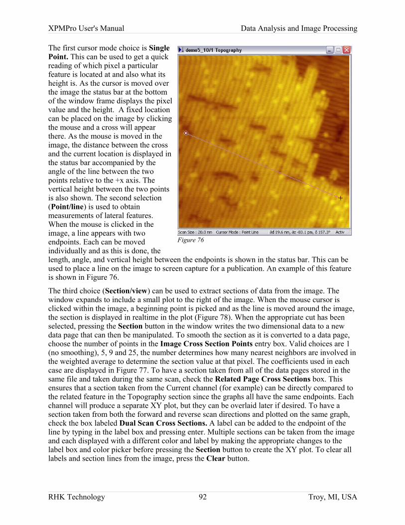
XPMPro User's Manual Data Analysis and Image Processing
The first cursor mode choice is Single Point. This can be used to get a quick reading of which pixel a particular feature is located at and also what its height is. As the cursor is moved over the image the status bar at the bottom of the window frame displays the pixel value and the height. A fixed location can be placed on the image by clicking the mouse and a cross will appear there. As the mouse is moved in the image, the distance between the cross and the current location is displayed in the status bar accompanied by the angle of the line between the two points relative to the +x axis. The vertical height between the two points is also shown. The second selection (Point/line) is used to obtain measurements of lateral features. When the mouse is clicked in the image, a line appears with two endpoints. Each can be moved individually and as this is done, the length, angle, and vertical height between the endpoints is shown in the status bar. This can be used to place a line on the image to screen capture for a publication. An example of this feature is shown in Figure 76.
The third choice (Section/view) can be used to extract sections of data from the image. The window expands to include a small plot to the right of the image. When the mouse cursor is clicked within the image, a beginning point is picked and as the line is moved around the image, the section is displayed in realtime in the plot (Figure 78). When the appropriate cut has been selected, pressing the Section button in the window writes the two dimensional data to a new data page that can then be manipulated. To smooth the section as it is converted to a data page, choose the number of points in the Image Cross Section Points entry box. Valid choices are 1 (no smoothing), 5, 9 and 25, the number determines how many nearest neighbors are involved in the weighted average to determine the section value at that pixel. The coefficients used in each case are displayed in Figure 77. To have a section taken from all of the data pages stored in the same file and taken during the same scan, check the Related Page Cross Sections box. This ensures that a section taken from the Current channel (for example) can be directly compared to the related feature in the Topography section since the graphs all have the same endpoints. Each channel will produce a separate XY plot, but they can be overlaid later if desired. To have a section taken from both the forward and reverse scan directions and plotted on the same graph, check the box labeled Dual Scan Cross Sections. A label can be added to the endpoint of the line by typing in the label box and pressing enter. Multiple sections can be taken from the image and each displayed with a different color and label by making the appropriate changes to the label box and color picker before pressing the Section button to create the XY plot. To clear all labels and section lines from the image, press the Clear button.
RHK Technology 92 Troy, MI, USA
Figure 76
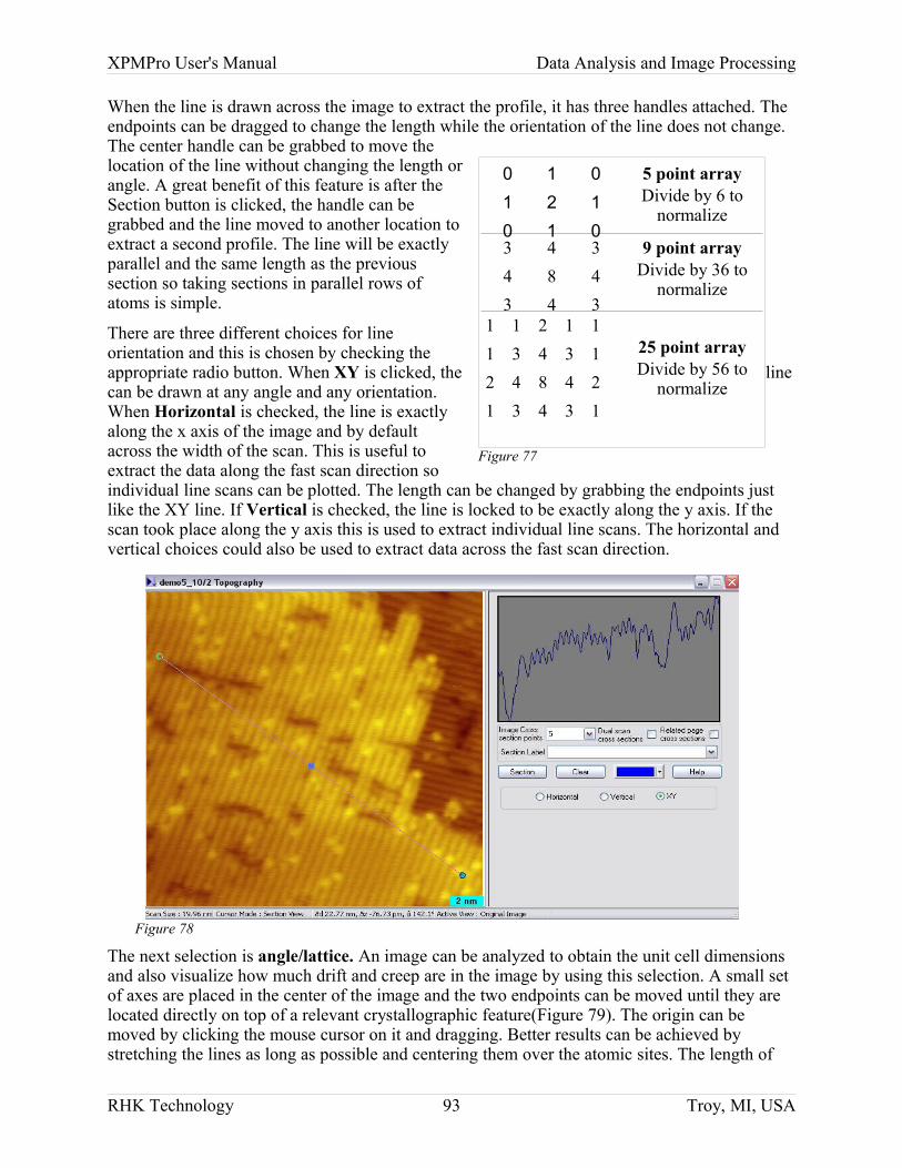
XPMPro User's Manual Data Analysis and Image Processing
When the line is drawn across the image to extract the profile, it has three handles attached. The endpoints can be dragged to change the length while the orientation of the line does not change. The center handle can be grabbed to move the location of the line without changing the length or angle. A great benefit of this feature is after the Section button is clicked, the handle can be grabbed and the line moved to another location to extract a second profile. The line will be exactly parallel and the same length as the previous section so taking sections in parallel rows of atoms is simple.
There are three different choices for line orientation and this is chosen by checking the appropriate radio button. When XY is clicked, the line can be drawn at any angle and any orientation. When Horizontal is checked, the line is exactly along the x axis of the image and by default across the width of the scan. This is useful to extract the data along the fast scan direction so individual line scans can be plotted. The length can be changed by grabbing the endpoints just like the XY line. If Vertical is checked, the line is locked to be exactly along the y axis. If the scan took place along the y axis this is used to extract individual line scans. The horizontal and vertical choices could also be used to extract data across the fast scan direction.
The next selection is angle/lattice. An image can be analyzed to obtain the unit cell dimensions and also visualize how much drift and creep are in the image by using this selection. A small set of axes are placed in the center of the image and the two endpoints can be moved until they are located directly on top of a relevant crystallographic feature(Figure 79). The origin can be moved by clicking the mouse cursor on it and dragging. Better results can be achieved by stretching the lines as long as possible and centering them over the atomic sites. The length of
RHK Technology 93 Troy, MI, USA
Figure 78
Figure 77
0 1 01 2 10 1 0
5 point arrayDivide by 6 to
normalize
3 4 34 8 43 4 3
9 point arrayDivide by 36 to
normalize
1 1 2 1 11 3 4 3 12 4 8 4 21 3 4 3 1
25 point arrayDivide by 56 to
normalize
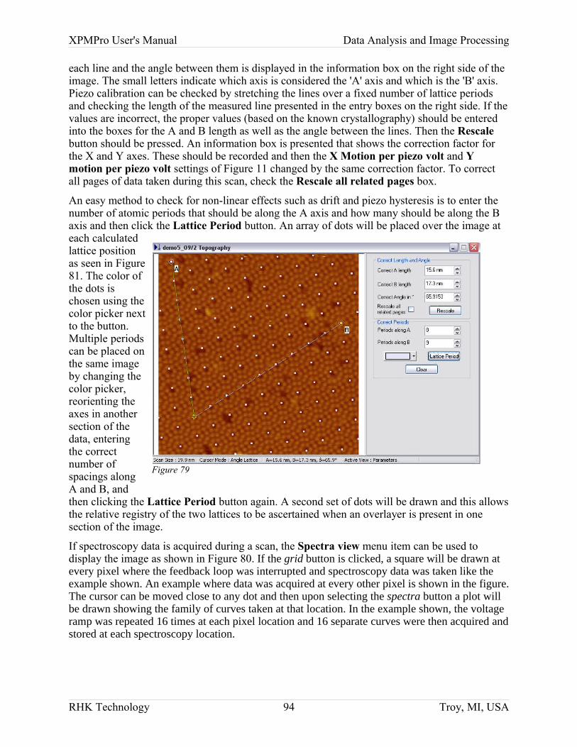
XPMPro User's Manual Data Analysis and Image Processing
each line and the angle between them is displayed in the information box on the right side of the image. The small letters indicate which axis is considered the 'A' axis and which is the 'B' axis. Piezo calibration can be checked by stretching the lines over a fixed number of lattice periods and checking the length of the measured line presented in the entry boxes on the right side. If the values are incorrect, the proper values (based on the known crystallography) should be entered into the boxes for the A and B length as well as the angle between the lines. Then the Rescale button should be pressed. An information box is presented that shows the correction factor for the X and Y axes. These should be recorded and then the X Motion per piezo volt and Y motion per piezo volt settings of Figure 11 changed by the same correction factor. To correct all pages of data taken during this scan, check the Rescale all related pages box.
An easy method to check for non-linear effects such as drift and piezo hysteresis is to enter the number of atomic periods that should be along the A axis and how many should be along the B axis and then click the Lattice Period button. An array of dots will be placed over the image at each calculated lattice position as seen in Figure 81. The color of the dots is chosen using the color picker next to the button. Multiple periods can be placed on the same image by changing the color picker, reorienting the axes in another section of the data, entering the correct number of spacings along A and B, and then clicking the Lattice Period button again. A second set of dots will be drawn and this allows the relative registry of the two lattices to be ascertained when an overlayer is present in one section of the image.
If spectroscopy data is acquired during a scan, the Spectra view menu item can be used to display the image as shown in Figure 80. If the grid button is clicked, a square will be drawn at every pixel where the feedback loop was interrupted and spectroscopy data was taken like the example shown. An example where data was acquired at every other pixel is shown in the figure. The cursor can be moved close to any dot and then upon selecting the spectra button a plot will be drawn showing the family of curves taken at that location. In the example shown, the voltage ramp was repeated 16 times at each pixel location and 16 separate curves were then acquired and stored at each spectroscopy location.
RHK Technology 94 Troy, MI, USA
Figure 79
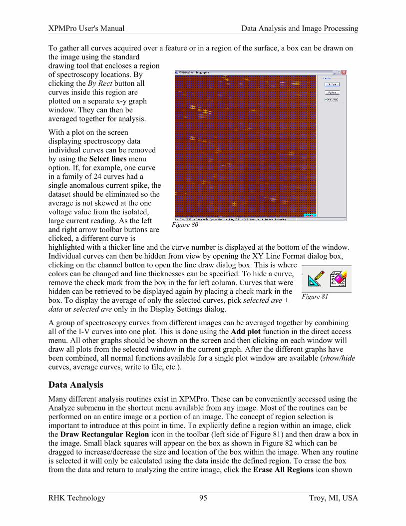
XPMPro User's Manual Data Analysis and Image Processing
To gather all curves acquired over a feature or in a region of the surface, a box can be drawn on the image using the standard drawing tool that encloses a region of spectroscopy locations. By clicking the By Rect button all curves inside this region are plotted on a separate x-y graph window. They can then be averaged together for analysis.
With a plot on the screen displaying spectroscopy data individual curves can be removed by using the Select lines menu option. If, for example, one curve in a family of 24 curves had a single anomalous current spike, the dataset should be eliminated so the average is not skewed at the one voltage value from the isolated, large current reading. As the left and right arrow toolbar buttons are clicked, a different curve is highlighted with a thicker line and the curve number is displayed at the bottom of the window. Individual curves can then be hidden from view by opening the XY Line Format dialog box, clicking on the channel button to open the line draw dialog box. This is where colors can be changed and line thicknesses can be specified. To hide a curve, remove the check mark from the box in the far left column. Curves that were hidden can be retrieved to be displayed again by placing a check mark in the box. To display the average of only the selected curves, pick selected ave + data or selected ave only in the Display Settings dialog.
A group of spectroscopy curves from different images can be averaged together by combining all of the I-V curves into one plot. This is done using the Add plot function in the direct access menu. All other graphs should be shown on the screen and then clicking on each window will draw all plots from the selected window in the current graph. After the different graphs have been combined, all normal functions available for a single plot window are available (show/hide curves, average curves, write to file, etc.).
Data AnalysisMany different analysis routines exist in XPMPro. These can be conveniently accessed using the Analyze submenu in the shortcut menu available from any image. Most of the routines can be performed on an entire image or a portion of an image. The concept of region selection is important to introduce at this point in time. To explicitly define a region within an image, click the Draw Rectangular Region icon in the toolbar (left side of Figure 81) and then draw a box in the image. Small black squares will appear on the box as shown in Figure 82 which can be dragged to increase/decrease the size and location of the box within the image. When any routine is selected it will only be calculated using the data inside the defined region. To erase the box from the data and return to analyzing the entire image, click the Erase All Regions icon shown
RHK Technology 95 Troy, MI, USA
Figure 81
Figure 80
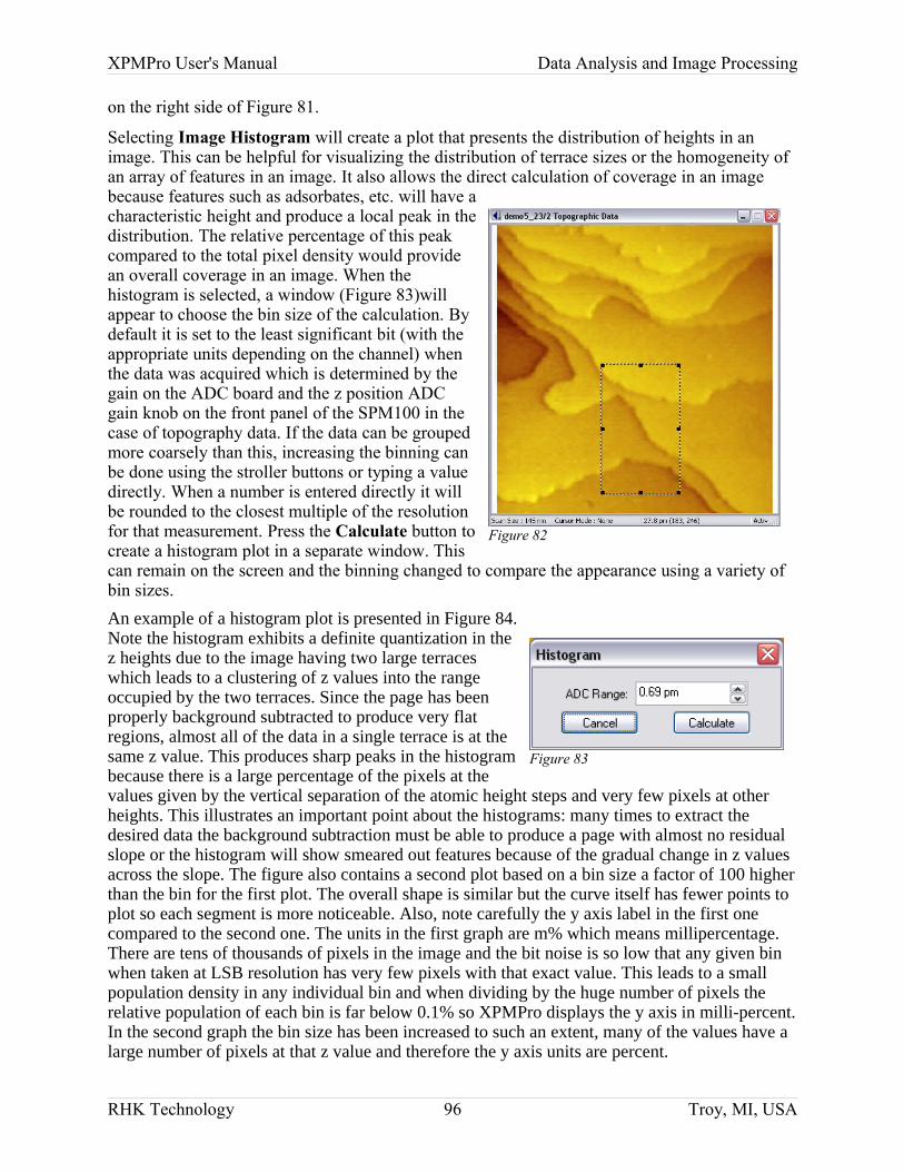
XPMPro User's Manual Data Analysis and Image Processing
on the right side of Figure 81.
Selecting Image Histogram will create a plot that presents the distribution of heights in an image. This can be helpful for visualizing the distribution of terrace sizes or the homogeneity of an array of features in an image. It also allows the direct calculation of coverage in an image because features such as adsorbates, etc. will have a characteristic height and produce a local peak in the distribution. The relative percentage of this peak compared to the total pixel density would provide an overall coverage in an image. When the histogram is selected, a window (Figure 83)will appear to choose the bin size of the calculation. By default it is set to the least significant bit (with the appropriate units depending on the channel) when the data was acquired which is determined by the gain on the ADC board and the z position ADC gain knob on the front panel of the SPM100 in the case of topography data. If the data can be grouped more coarsely than this, increasing the binning can be done using the stroller buttons or typing a value directly. When a number is entered directly it will be rounded to the closest multiple of the resolution for that measurement. Press the Calculate button to create a histogram plot in a separate window. This can remain on the screen and the binning changed to compare the appearance using a variety of bin sizes.An example of a histogram plot is presented in Figure 84. Note the histogram exhibits a definite quantization in the z heights due to the image having two large terraces which leads to a clustering of z values into the range occupied by the two terraces. Since the page has been properly background subtracted to produce very flat regions, almost all of the data in a single terrace is at the same z value. This produces sharp peaks in the histogram because there is a large percentage of the pixels at the values given by the vertical separation of the atomic height steps and very few pixels at other heights. This illustrates an important point about the histograms: many times to extract the desired data the background subtraction must be able to produce a page with almost no residual slope or the histogram will show smeared out features because of the gradual change in z values across the slope. The figure also contains a second plot based on a bin size a factor of 100 higher than the bin for the first plot. The overall shape is similar but the curve itself has fewer points to plot so each segment is more noticeable. Also, note carefully the y axis label in the first one compared to the second one. The units in the first graph are m% which means millipercentage. There are tens of thousands of pixels in the image and the bit noise is so low that any given bin when taken at LSB resolution has very few pixels with that exact value. This leads to a small population density in any individual bin and when dividing by the huge number of pixels the relative population of each bin is far below 0.1% so XPMPro displays the y axis in milli-percent. In the second graph the bin size has been increased to such an extent, many of the values have a large number of pixels at that z value and therefore the y axis units are percent.
RHK Technology 96 Troy, MI, USA
Figure 83
Figure 82
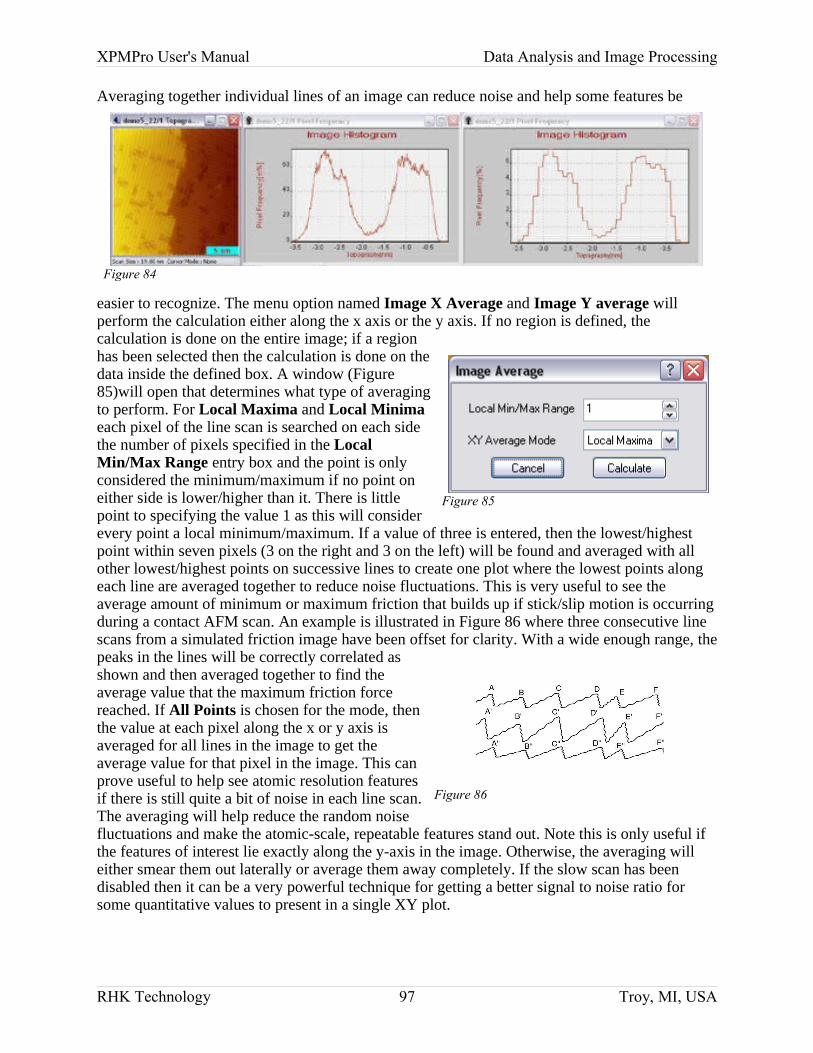
XPMPro User's Manual Data Analysis and Image Processing
Averaging together individual lines of an image can reduce noise and help some features be
easier to recognize. The menu option named Image X Average and Image Y average will perform the calculation either along the x axis or the y axis. If no region is defined, the calculation is done on the entire image; if a region has been selected then the calculation is done on the data inside the defined box. A window (Figure85)will open that determines what type of averaging to perform. For Local Maxima and Local Minima each pixel of the line scan is searched on each side the number of pixels specified in the Local Min/Max Range entry box and the point is only considered the minimum/maximum if no point on either side is lower/higher than it. There is little point to specifying the value 1 as this will consider every point a local minimum/maximum. If a value of three is entered, then the lowest/highest point within seven pixels (3 on the right and 3 on the left) will be found and averaged with all other lowest/highest points on successive lines to create one plot where the lowest points along each line are averaged together to reduce noise fluctuations. This is very useful to see the average amount of minimum or maximum friction that builds up if stick/slip motion is occurring during a contact AFM scan. An example is illustrated in Figure 86 where three consecutive line scans from a simulated friction image have been offset for clarity. With a wide enough range, the peaks in the lines will be correctly correlated as shown and then averaged together to find the average value that the maximum friction force reached. If All Points is chosen for the mode, then the value at each pixel along the x or y axis is averaged for all lines in the image to get the average value for that pixel in the image. This can prove useful to help see atomic resolution features if there is still quite a bit of noise in each line scan. The averaging will help reduce the random noise fluctuations and make the atomic-scale, repeatable features stand out. Note this is only useful if the features of interest lie exactly along the y-axis in the image. Otherwise, the averaging will either smear them out laterally or average them away completely. If the slow scan has been disabled then it can be a very powerful technique for getting a better signal to noise ratio for some quantitative values to present in a single XY plot.
RHK Technology 97 Troy, MI, USA
Figure 85
Figure 86
Figure 84
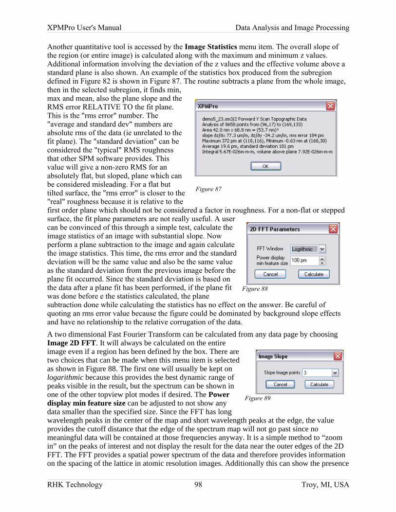
XPMPro User's Manual Data Analysis and Image Processing
Another quantitative tool is accessed by the Image Statistics menu item. The overall slope of the region (or entire image) is calculated along with the maximum and minimum z values. Additional information involving the deviation of the z values and the effective volume above a standard plane is also shown. An example of the statistics box produced from the subregion defined in Figure 82 is shown in Figure 87. The routine subtracts a plane from the whole image, then in the selected subregion, it finds min, max and mean, also the plane slope and the RMS error RELATIVE TO the fit plane. This is the "rms error" number. The "average and standard dev" numbers are absolute rms of the data (ie unrelated to the fit plane). The "standard deviation" can be considered the "typical" RMS roughness that other SPM software provides. This value will give a non-zero RMS for an absolutely flat, but sloped, plane which can be considered misleading. For a flat but tilted surface, the "rms error" is closer to the "real" roughness because it is relative to the first order plane which should not be considered a factor in roughness. For a non-flat or stepped surface, the fit plane parameters are not really useful. A user can be convinced of this through a simple test, calculate the image statistics of an image with substantial slope. Now perform a plane subtraction to the image and again calculate the image statistics. This time, the rms error and the standard deviation will be the same value and also be the same value as the standard deviation from the previous image before the plane fit occurred. Since the standard deviation is based on the data after a plane fit has been performed, if the plane fit was done before e the statistics calculated, the plane subtraction done while calculating the statistics has no effect on the answer. Be careful of quoting an rms error value because the figure could be dominated by background slope effects and have no relationship to the relative corrugation of the data.A two dimensional Fast Fourier Transform can be calculated from any data page by choosing Image 2D FFT. It will always be calculated on the entire image even if a region has been defined by the box. There are two choices that can be made when this menu item is selected as shown in Figure 88. The first one will usually be kept on logarithmic because this provides the best dynamic range of peaks visible in the result, but the spectrum can be shown in one of the other topview plot modes if desired. The Power display min feature size can be adjusted to not show any data smaller than the specified size. Since the FFT has long wavelength peaks in the center of the map and short wavelength peaks at the edge, the value provides the cutoff distance that the edge of the spectrum map will not go past since no meaningful data will be contained at those frequencies anyway. It is a simple method to “zoom in” on the peaks of interest and not display the result for the data near the outer edges of the 2D FFT. The FFT provides a spatial power spectrum of the data and therefore provides information on the spacing of the lattice in atomic resolution images. Additionally this can show the presence
RHK Technology 98 Troy, MI, USA
Figure 87
Figure 89
Figure 88
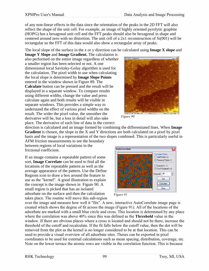
XPMPro User's Manual Data Analysis and Image Processing
of any non-linear effects in the data since the orientation of the peaks in the 2D FFT will also reflect the shape of the unit cell. For example, an image of highly oriented pyrolytic graphite (HOPG) has a hexagonal unit cell and the FFT peaks should also be hexagonal in shape and centered around zero with no distortion. The unit cell of a 2x1 reconstruction of Si(001) will be rectangular so the FFT of this data would also show a rectangular array of peaks.
The local slope of the surface in the x or y direction can be calculated using Image X slope and Image Y Slope and Image Gradient. The calculation is also performed on the entire image regardless of whether a smaller region has been selected or not. A one dimensional local Savitzky-Golay algorithm is used for the calculation. The pixel width to use when calculating the local slope is determined by Image Slope Points entered in the window shown in Figure 89. The Calculate button can be pressed and the result will be displayed in a separate window. To compare results using different widths, change the value and press calculate again and both results will be visible in separate windows. This provides a simple way to understand the effect of various pixel widths on the result. The wider the pixel value, the smoother the derivative will be, but a loss in detail will also take place. The derivative of each line of data in the correct direction is calculated and an image formed by combining the differentiated lines. When Image Gradient is chosen, the slope in the X and Y directions are both calculated on a pixel by pixel basis and the image is a representation of the two slopes combined. This is particularly useful in AFM friction measurements to see the boundary between regions of local variations in the frictional coefficient.
If an image contains a repeatable pattern of some sort, Image Correlate can be used to find all the locations of the repeatable pattern as well as the average appearance of the pattern. Use the Define Regions icon to draw a box around the feature to use as the "kernel". A good illustration to explain the concept is the image shown in Figure 90. A small region is picked that has an isolated adsorbate on the surface and then the calculation takes place. The routine will move this sub-region over the image and measure how well it "fits". A new, interactive AutoCorrelate image page is created which shows the degree of fit across the image (Figure 91). All of the locations of the adsorbate are marked with a small blue circle and cross. This location is determined by any place where the correlation was above 40% since this was defined as the Threshold value in the window. If there are obvious places where a cross is located and should not be there, increase the threshold of the cutoff and recalculate. If the fit falls below the cutoff value, then the dot will be removed from the plot as the kernel is no longer considered to be at that location. This can be used to provide a visual overview of all adsorbate sites. Theses can be exported in pixel coordinates to be used for external calculations such as mean spacing, distribution, coverage, etc. Note on the lower terrace the atomic rows are visible in the correlation function. This is because
RHK Technology 99 Troy, MI, USA
Figure 90
Figure 91
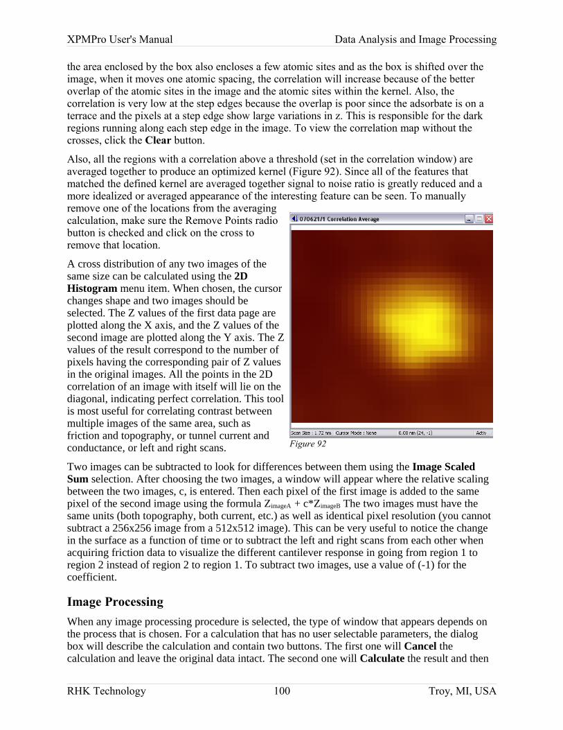
XPMPro User's Manual Data Analysis and Image Processing
the area enclosed by the box also encloses a few atomic sites and as the box is shifted over the image, when it moves one atomic spacing, the correlation will increase because of the better overlap of the atomic sites in the image and the atomic sites within the kernel. Also, the correlation is very low at the step edges because the overlap is poor since the adsorbate is on a terrace and the pixels at a step edge show large variations in z. This is responsible for the dark regions running along each step edge in the image. To view the correlation map without the crosses, click the Clear button.
Also, all the regions with a correlation above a threshold (set in the correlation window) are averaged together to produce an optimized kernel (Figure 92). Since all of the features that matched the defined kernel are averaged together signal to noise ratio is greatly reduced and a more idealized or averaged appearance of the interesting feature can be seen. To manually remove one of the locations from the averaging calculation, make sure the Remove Points radio button is checked and click on the cross to remove that location.
A cross distribution of any two images of the same size can be calculated using the 2D Histogram menu item. When chosen, the cursor changes shape and two images should be selected. The Z values of the first data page are plotted along the X axis, and the Z values of the second image are plotted along the Y axis. The Z values of the result correspond to the number of pixels having the corresponding pair of Z values in the original images. All the points in the 2D correlation of an image with itself will lie on the diagonal, indicating perfect correlation. This tool is most useful for correlating contrast between multiple images of the same area, such as friction and topography, or tunnel current and conductance, or left and right scans.
Two images can be subtracted to look for differences between them using the Image Scaled Sum selection. After choosing the two images, a window will appear where the relative scaling between the two images, c, is entered. Then each pixel of the first image is added to the same pixel of the second image using the formula ZimageA + c*ZimageB The two images must have the same units (both topography, both current, etc.) as well as identical pixel resolution (you cannot subtract a 256x256 image from a 512x512 image). This can be very useful to notice the change in the surface as a function of time or to subtract the left and right scans from each other when acquiring friction data to visualize the different cantilever response in going from region 1 to region 2 instead of region 2 to region 1. To subtract two images, use a value of (-1) for the coefficient.
Image ProcessingWhen any image processing procedure is selected, the type of window that appears depends on the process that is chosen. For a calculation that has no user selectable parameters, the dialog box will describe the calculation and contain two buttons. The first one will Cancel the calculation and leave the original data intact. The second one will Calculate the result and then
RHK Technology 100 Troy, MI, USA
Figure 92
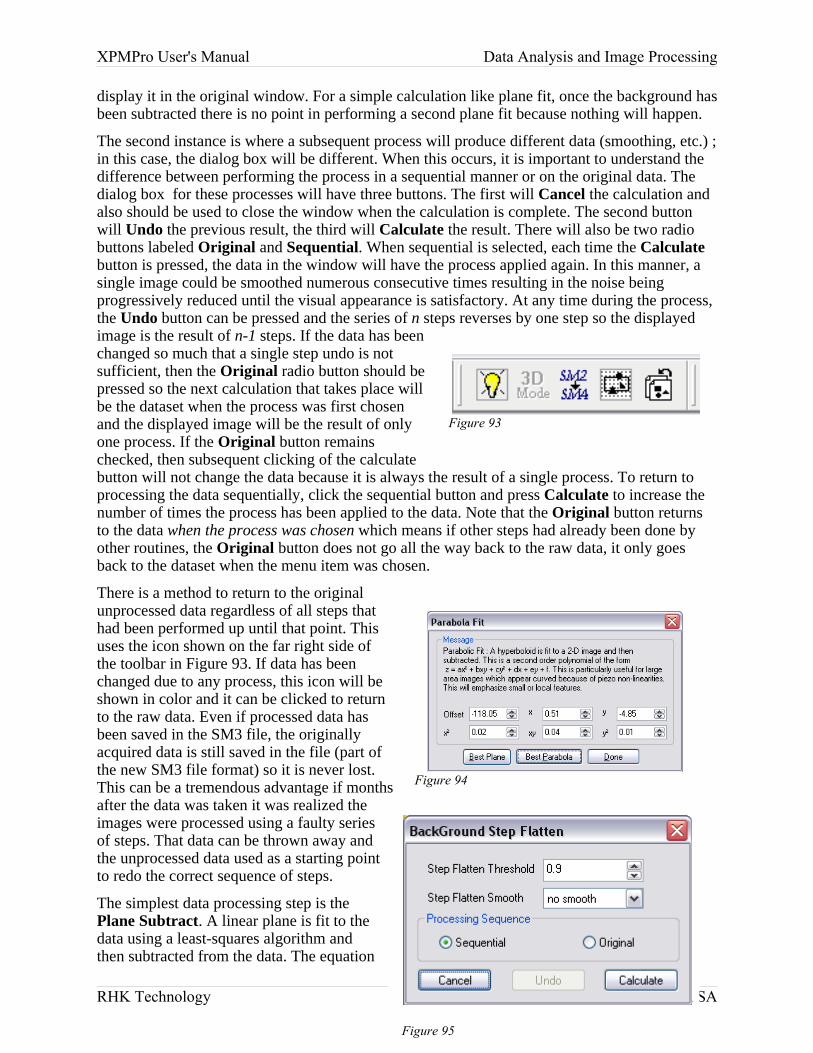
XPMPro User's Manual Data Analysis and Image Processing
display it in the original window. For a simple calculation like plane fit, once the background has been subtracted there is no point in performing a second plane fit because nothing will happen.
The second instance is where a subsequent process will produce different data (smoothing, etc.) ; in this case, the dialog box will be different. When this occurs, it is important to understand the difference between performing the process in a sequential manner or on the original data. The dialog box for these processes will have three buttons. The first will Cancel the calculation and also should be used to close the window when the calculation is complete. The second button will Undo the previous result, the third will Calculate the result. There will also be two radio buttons labeled Original and Sequential. When sequential is selected, each time the Calculate button is pressed, the data in the window will have the process applied again. In this manner, a single image could be smoothed numerous consecutive times resulting in the noise being progressively reduced until the visual appearance is satisfactory. At any time during the process, the Undo button can be pressed and the series of n steps reverses by one step so the displayed image is the result of n-1 steps. If the data has been changed so much that a single step undo is not sufficient, then the Original radio button should be pressed so the next calculation that takes place will be the dataset when the process was first chosen and the displayed image will be the result of only one process. If the Original button remains checked, then subsequent clicking of the calculate button will not change the data because it is always the result of a single process. To return to processing the data sequentially, click the sequential button and press Calculate to increase the number of times the process has been applied to the data. Note that the Original button returns to the data when the process was chosen which means if other steps had already been done by other routines, the Original button does not go all the way back to the raw data, it only goes back to the dataset when the menu item was chosen.
There is a method to return to the original unprocessed data regardless of all steps that had been performed up until that point. This uses the icon shown on the far right side of the toolbar in Figure 93. If data has been changed due to any process, this icon will be shown in color and it can be clicked to return to the raw data. Even if processed data has been saved in the SM3 file, the originally acquired data is still saved in the file (part of the new SM3 file format) so it is never lost. This can be a tremendous advantage if months after the data was taken it was realized the images were processed using a faulty series of steps. That data can be thrown away and the unprocessed data used as a starting point to redo the correct sequence of steps.
The simplest data processing step is the Plane Subtract. A linear plane is fit to the data using a least-squares algorithm and then subtracted from the data. The equation
RHK Technology 101 Troy, MI, USA
Figure 93
Figure 94
Figure 95

XPMPro User's Manual Data Analysis and Image Processing
used is ax+by+c. It only makes sense to perform this one time on any piece of data. A slightly better routine for some data is found using the Parabola Subtract where a two dimensional hyperboloid is fit to the data and then subtracted. This can help eliminate effects present when scanning large distance using tube scanners due to the curved surface the scan plane follows. The equation used is ax2+bxy+cy2+dx+ey+f. This step also only makes sense to be performed once. To open the window shown in Figure 94, right click on an image and choose Process/Background/Parabola Subtract. When the window first opens the coefficients are all equal to zero. To have the software automatically subtract the best fit plane or best fit parabola, click the appropriate button. At any time, the individual controls can be changed to have manual control over the subtracted background. Of course, if the second order terms are all set yo zero, then a plane will be defined and subtracted from the image. If other derived data is present on the screen (sections, histograms, 3D renderings, etc.) as the background subtraction coefficients are altered manually, the other data representations of the image will also update in real time. Often it is easier to decide the best subtraction by looking at a section or the histogram, particularly when the image has steps in it, by using this other data. When the line section shows flat terraces and when the histogram shows distinct peaks the image will accurately represent the real surface with terraces separated by the correct value based on the know crystallography.
Instead of manually adjusting the background of a terraced surface, the built in Step Flatten routine can be used to get an image with flat terraces from an area of the surface containing steps. This routine fits a parabola to the flat terraces only. When the dialog box (Figure 95) is opened for this process, it is recommended to leave the Original button checked so the calculation is performed on the raw data each time (as the settings are tweaked for optimal results) instead of “flattening” an image that has already been flattened. After changing either or both parameters click the Calculate button to perform the function and view the new result in the original window. The Step Flatten Threshold determines how flat a “flat” terrace must be in order to contribute to the calculation. Too small of a value here will result in an unstable calculation, but too large will not achieve the desired result. For images with broad terraces and few steps, try a value greater than one. Step Flatten Smooth determines the number of pixels to use to determine if a region of the surface is smooth or lies at a step. The smaller the number, the longer the calculation time. This algorithm was graciously provided by Dr. James C. Dunphy.
If X Offset Subtract is chosen, the mean value of each line is subtracted on a line-by-line basis for all data along the x axis, and this can be used to reduce low frequency noise in the data. The average value of the entire data page is kept constant though since there are cases where this value has physical meaning. This is most commonly used to remove offset in an image due to an instantaneous tip change where the z piezo adjusts up or down a significant amount because the overall length of the tip has changed when scanning along the x axis. To remove the slope of each line of data along the x axis, use X Slope Subtract. However, it is far superior to use the hardware slope compensation to remove as much slope as possible along the fast scan direction before the ADC when acquiring topographic data. Since this is not possible for any other data channel, the image processing step is quite useful for those images.
If Y Offset Subtract is chosen, the mean value of each line is subtracted on a line-by-line basis for all data along the y axis, and this can be used to reduce low frequency noise in the data. The average value of the entire data page is kept constant though since there are cases where this value has physical meaning. This is most commonly used to remove offset in an image due to an instantaneous tip change where the z piezo adjusts up or down a significant amount because the overall length of the tip has changed when scanning along the y axis. To remove the slope of each line of data along the y axis, use Y Slope Subtract. However, it is far superior to use the hardware slope compensation to remove as much slope as possible along the fast scan direction
RHK Technology 102 Troy, MI, USA
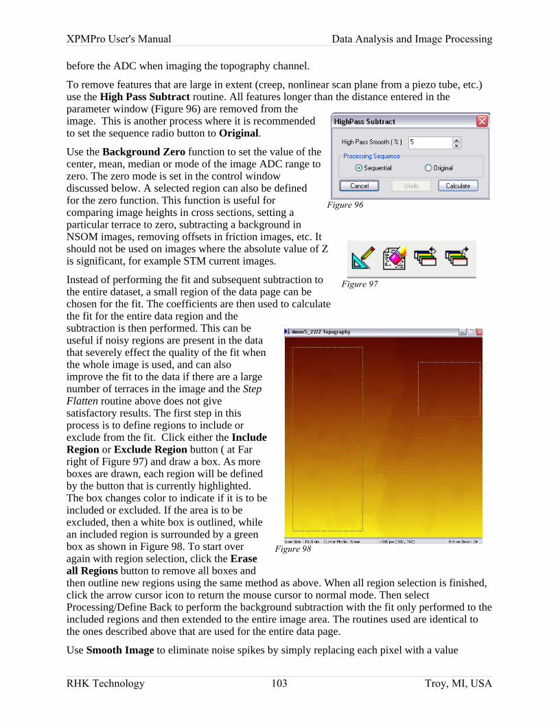
XPMPro User's Manual Data Analysis and Image Processing
before the ADC when imaging the topography channel.
To remove features that are large in extent (creep, nonlinear scan plane from a piezo tube, etc.) use the High Pass Subtract routine. All features longer than the distance entered in the parameter window (Figure 96) are removed from the image. This is another process where it is recommended to set the sequence radio button to Original.
Use the Background Zero function to set the value of the center, mean, median or mode of the image ADC range to zero. The zero mode is set in the control window discussed below. A selected region can also be defined for the zero function. This function is useful for comparing image heights in cross sections, setting a particular terrace to zero, subtracting a background in NSOM images, removing offsets in friction images, etc. It should not be used on images where the absolute value of Z is significant, for example STM current images.
Instead of performing the fit and subsequent subtraction to the entire dataset, a small region of the data page can be chosen for the fit. The coefficients are then used to calculate the fit for the entire data region and the subtraction is then performed. This can be useful if noisy regions are present in the data that severely effect the quality of the fit when the whole image is used, and can also improve the fit to the data if there are a large number of terraces in the image and the Step Flatten routine above does not give satisfactory results. The first step in this process is to define regions to include or exclude from the fit. Click either the Include Region or Exclude Region button ( at Far right of Figure 97) and draw a box. As more boxes are drawn, each region will be defined by the button that is currently highlighted. The box changes color to indicate if it is to be included or excluded. If the area is to be excluded, then a white box is outlined, while an included region is surrounded by a green box as shown in Figure 98. To start over again with region selection, click the Erase all Regions button to remove all boxes and then outline new regions using the same method as above. When all region selection is finished, click the arrow cursor icon to return the mouse cursor to normal mode. Then select Processing/Define Back to perform the background subtraction with the fit only performed to the included regions and then extended to the entire image area. The routines used are identical to the ones described above that are used for the entire data page.
Use Smooth Image to eliminate noise spikes by simply replacing each pixel with a value
RHK Technology 103 Troy, MI, USA
Figure 96
Figure 97
Figure 98
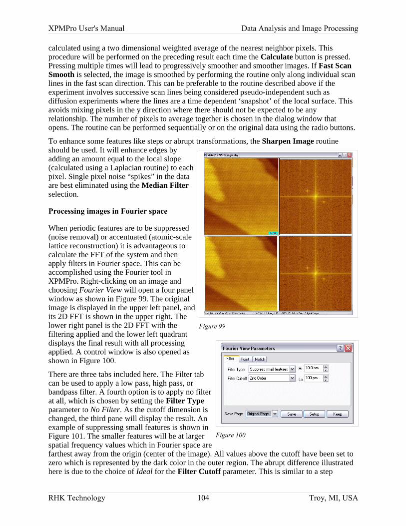
XPMPro User's Manual Data Analysis and Image Processing
calculated using a two dimensional weighted average of the nearest neighbor pixels. This procedure will be performed on the preceding result each time the Calculate button is pressed. Pressing multiple times will lead to progressively smoother and smoother images. If Fast Scan Smooth is selected, the image is smoothed by performing the routine only along individual scan lines in the fast scan direction. This can be preferable to the routine described above if the experiment involves successive scan lines being considered pseudo-independent such as diffusion experiments where the lines are a time dependent ‘snapshot’ of the local surface. This avoids mixing pixels in the y direction where there should not be expected to be any relationship. The number of pixels to average together is chosen in the dialog window that opens. The routine can be performed sequentially or on the original data using the radio buttons.
To enhance some features like steps or abrupt transformations, the Sharpen Image routine should be used. It will enhance edges by adding an amount equal to the local slope (calculated using a Laplacian routine) to each pixel. Single pixel noise “spikes” in the data are best eliminated using the Median Filter selection.
Processing images in Fourier space
When periodic features are to be suppressed (noise removal) or accentuated (atomic-scale lattice reconstruction) it is advantageous to calculate the FFT of the system and then apply filters in Fourier space. This can be accomplished using the Fourier tool in XPMPro. Right-clicking on an image and choosing Fourier View will open a four panel window as shown in Figure 99. The original image is displayed in the upper left panel, and its 2D FFT is shown in the upper right. The lower right panel is the 2D FFT with the filtering applied and the lower left quadrant displays the final result with all processing applied. A control window is also opened as shown in Figure 100.
There are three tabs included here. The Filter tab can be used to apply a low pass, high pass, or bandpass filter. A fourth option is to apply no filter at all, which is chosen by setting the Filter Type parameter to No Filter. As the cutoff dimension is changed, the third pane will display the result. An example of suppressing small features is shown in Figure 101. The smaller features will be at larger spatial frequency values which in Fourier space are farthest away from the origin (center of the image). All values above the cutoff have been set to zero which is represented by the dark color in the outer region. The abrupt difference illustrated here is due to the choice of Ideal for the Filter Cutoff parameter. This is similar to a step
RHK Technology 104 Troy, MI, USA
Figure 100
Figure 99
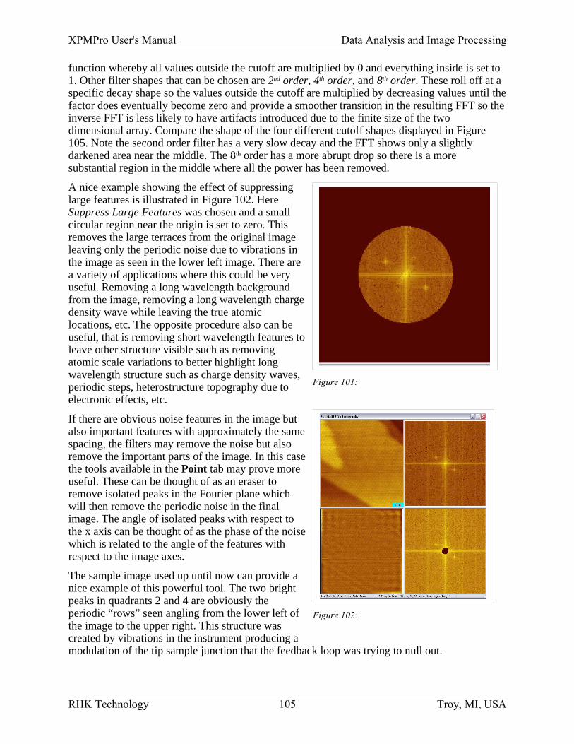
XPMPro User's Manual Data Analysis and Image Processing
function whereby all values outside the cutoff are multiplied by 0 and everything inside is set to 1. Other filter shapes that can be chosen are 2nd order, 4th order, and 8th order. These roll off at a specific decay shape so the values outside the cutoff are multiplied by decreasing values until the factor does eventually become zero and provide a smoother transition in the resulting FFT so the inverse FFT is less likely to have artifacts introduced due to the finite size of the two dimensional array. Compare the shape of the four different cutoff shapes displayed in Figure105. Note the second order filter has a very slow decay and the FFT shows only a slightly darkened area near the middle. The 8th order has a more abrupt drop so there is a more substantial region in the middle where all the power has been removed.
A nice example showing the effect of suppressing large features is illustrated in Figure 102. Here Suppress Large Features was chosen and a small circular region near the origin is set to zero. This removes the large terraces from the original image leaving only the periodic noise due to vibrations in the image as seen in the lower left image. There are a variety of applications where this could be very useful. Removing a long wavelength background from the image, removing a long wavelength charge density wave while leaving the true atomic locations, etc. The opposite procedure also can be useful, that is removing short wavelength features to leave other structure visible such as removing atomic scale variations to better highlight long wavelength structure such as charge density waves, periodic steps, heterostructure topography due to electronic effects, etc.
If there are obvious noise features in the image but also important features with approximately the same spacing, the filters may remove the noise but also remove the important parts of the image. In this case the tools available in the Point tab may prove more useful. These can be thought of as an eraser to remove isolated peaks in the Fourier plane which will then remove the periodic noise in the final image. The angle of isolated peaks with respect to the x axis can be thought of as the phase of the noise which is related to the angle of the features with respect to the image axes.
The sample image used up until now can provide a nice example of this powerful tool. The two bright peaks in quadrants 2 and 4 are obviously the periodic “rows” seen angling from the lower left of the image to the upper right. This structure was created by vibrations in the instrument producing a modulation of the tip sample junction that the feedback loop was trying to null out.
RHK Technology 105 Troy, MI, USA
Figure 102:
Figure 101:
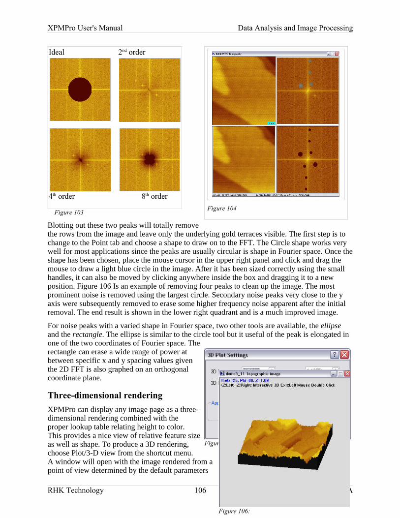
XPMPro User's Manual Data Analysis and Image Processing
Blotting out these two peaks will totally remove the rows from the image and leave only the underlying gold terraces visible. The first step is to change to the Point tab and choose a shape to draw on to the FFT. The Circle shape works very well for most applications since the peaks are usually circular is shape in Fourier space. Once the shape has been chosen, place the mouse cursor in the upper right panel and click and drag the mouse to draw a light blue circle in the image. After it has been sized correctly using the small handles, it can also be moved by clicking anywhere inside the box and dragging it to a new position. Figure 106 Is an example of removing four peaks to clean up the image. The most prominent noise is removed using the largest circle. Secondary noise peaks very close to the y axis were subsequently removed to erase some higher frequency noise apparent after the initial removal. The end result is shown in the lower right quadrant and is a much improved image.
For noise peaks with a varied shape in Fourier space, two other tools are available, the ellipse and the rectangle. The ellipse is similar to the circle tool but it useful of the peak is elongated in one of the two coordinates of Fourier space. The rectangle can erase a wide range of power at between specific x and y spacing values given the 2D FFT is also graphed on an orthogonal coordinate plane.
Three-dimensional renderingXPMPro can display any image page as a three-dimensional rendering combined with the proper lookup table relating height to color. This provides a nice view of relative feature size as well as shape. To produce a 3D rendering, choose Plot/3-D view from the shortcut menu. A window will open with the image rendered from a point of view determined by the default parameters
RHK Technology 106 Troy, MI, USA
Figure 103
Ideal 2nd order
4th order 8th orderFigure 104
Figure 105:
Figure 106:
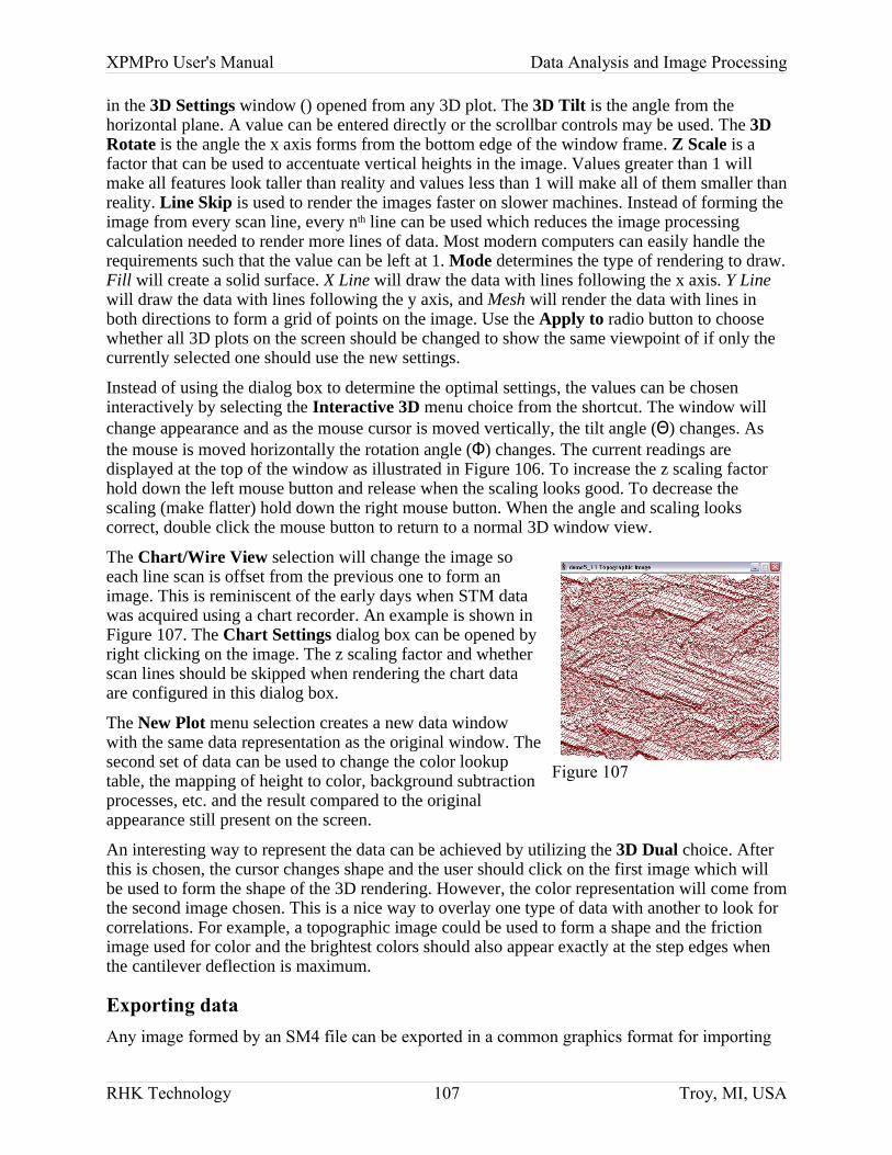
XPMPro User's Manual Data Analysis and Image Processing
in the 3D Settings window () opened from any 3D plot. The 3D Tilt is the angle from the horizontal plane. A value can be entered directly or the scrollbar controls may be used. The 3D Rotate is the angle the x axis forms from the bottom edge of the window frame. Z Scale is a factor that can be used to accentuate vertical heights in the image. Values greater than 1 will make all features look taller than reality and values less than 1 will make all of them smaller than reality. Line Skip is used to render the images faster on slower machines. Instead of forming the image from every scan line, every nth line can be used which reduces the image processing calculation needed to render more lines of data. Most modern computers can easily handle the requirements such that the value can be left at 1. Mode determines the type of rendering to draw. Fill will create a solid surface. X Line will draw the data with lines following the x axis. Y Line will draw the data with lines following the y axis, and Mesh will render the data with lines in both directions to form a grid of points on the image. Use the Apply to radio button to choose whether all 3D plots on the screen should be changed to show the same viewpoint of if only the currently selected one should use the new settings.
Instead of using the dialog box to determine the optimal settings, the values can be chosen interactively by selecting the Interactive 3D menu choice from the shortcut. The window will change appearance and as the mouse cursor is moved vertically, the tilt angle (Θ) changes. As the mouse is moved horizontally the rotation angle (Φ) changes. The current readings are displayed at the top of the window as illustrated in Figure 106. To increase the z scaling factor hold down the left mouse button and release when the scaling looks good. To decrease the scaling (make flatter) hold down the right mouse button. When the angle and scaling looks correct, double click the mouse button to return to a normal 3D window view.
The Chart/Wire View selection will change the image so each line scan is offset from the previous one to form an image. This is reminiscent of the early days when STM data was acquired using a chart recorder. An example is shown in Figure 107. The Chart Settings dialog box can be opened by right clicking on the image. The z scaling factor and whether scan lines should be skipped when rendering the chart data are configured in this dialog box.
The New Plot menu selection creates a new data window with the same data representation as the original window. The second set of data can be used to change the color lookup table, the mapping of height to color, background subtraction processes, etc. and the result compared to the original appearance still present on the screen.
An interesting way to represent the data can be achieved by utilizing the 3D Dual choice. After this is chosen, the cursor changes shape and the user should click on the first image which will be used to form the shape of the 3D rendering. However, the color representation will come from the second image chosen. This is a nice way to overlay one type of data with another to look for correlations. For example, a topographic image could be used to form a shape and the friction image used for color and the brightest colors should also appear exactly at the step edges when the cantilever deflection is maximum.
Exporting dataAny image formed by an SM4 file can be exported in a common graphics format for importing
RHK Technology 107 Troy, MI, USA
Figure 107
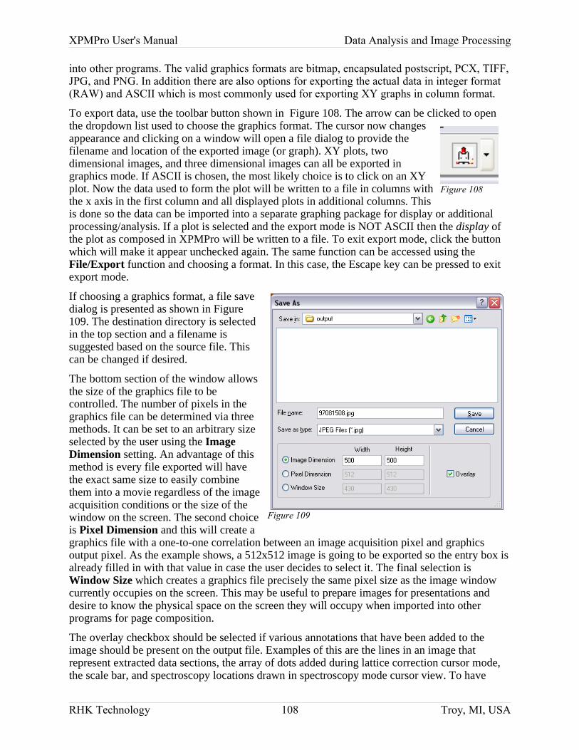
XPMPro User's Manual Data Analysis and Image Processing
into other programs. The valid graphics formats are bitmap, encapsulated postscript, PCX, TIFF, JPG, and PNG. In addition there are also options for exporting the actual data in integer format (RAW) and ASCII which is most commonly used for exporting XY graphs in column format.
To export data, use the toolbar button shown in Figure 108. The arrow can be clicked to open the dropdown list used to choose the graphics format. The cursor now changes appearance and clicking on a window will open a file dialog to provide the filename and location of the exported image (or graph). XY plots, two dimensional images, and three dimensional images can all be exported in graphics mode. If ASCII is chosen, the most likely choice is to click on an XY plot. Now the data used to form the plot will be written to a file in columns with the x axis in the first column and all displayed plots in additional columns. This is done so the data can be imported into a separate graphing package for display or additional processing/analysis. If a plot is selected and the export mode is NOT ASCII then the display of the plot as composed in XPMPro will be written to a file. To exit export mode, click the button which will make it appear unchecked again. The same function can be accessed using the File/Export function and choosing a format. In this case, the Escape key can be pressed to exit export mode.
If choosing a graphics format, a file save dialog is presented as shown in Figure109. The destination directory is selected in the top section and a filename is suggested based on the source file. This can be changed if desired.
The bottom section of the window allows the size of the graphics file to be controlled. The number of pixels in the graphics file can be determined via three methods. It can be set to an arbitrary size selected by the user using the Image Dimension setting. An advantage of this method is every file exported will have the exact same size to easily combine them into a movie regardless of the image acquisition conditions or the size of the window on the screen. The second choice is Pixel Dimension and this will create a graphics file with a one-to-one correlation between an image acquisition pixel and graphics output pixel. As the example shows, a 512x512 image is going to be exported so the entry box is already filled in with that value in case the user decides to select it. The final selection is Window Size which creates a graphics file precisely the same pixel size as the image window currently occupies on the screen. This may be useful to prepare images for presentations and desire to know the physical space on the screen they will occupy when imported into other programs for page composition.
The overlay checkbox should be selected if various annotations that have been added to the image should be present on the output file. Examples of this are the lines in an image that represent extracted data sections, the array of dots added during lattice correction cursor mode, the scale bar, and spectroscopy locations drawn in spectroscopy mode cursor view. To have
RHK Technology 108 Troy, MI, USA
Figure 108
Figure 109

XPMPro User's Manual Data Analysis and Image Processing
purely the image pixels only, leave this box unchecked.
RHK Technology 109 Troy, MI, USA

XPMPro User's Manual Data Acquisition Techniques
Advanced Techniques
RHK Technology 110 Troy, MI, USA
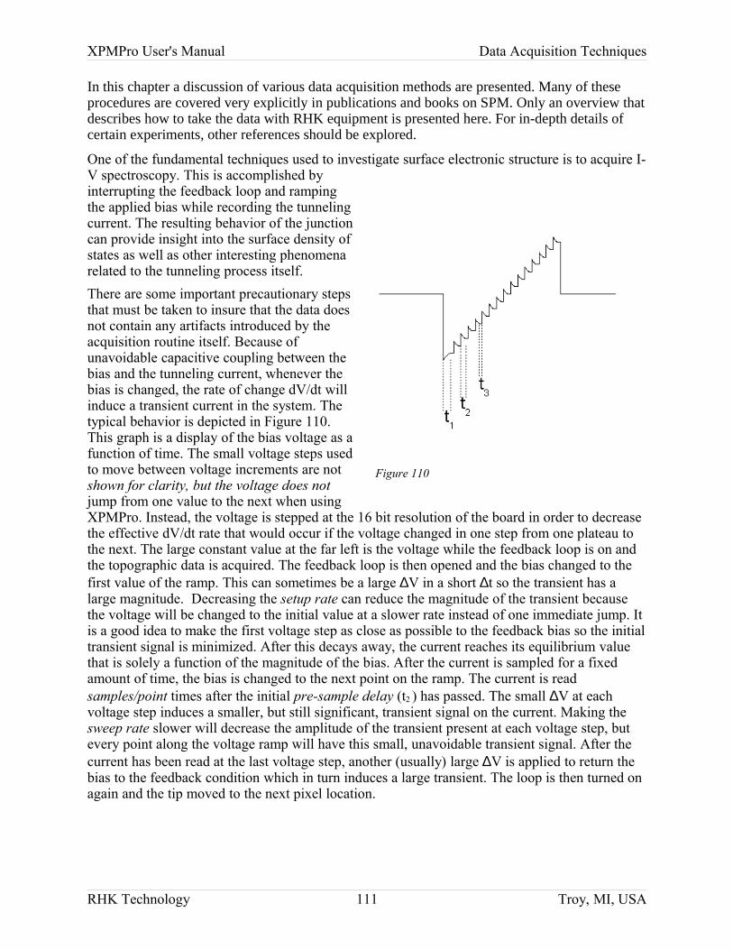
XPMPro User's Manual Data Acquisition Techniques
In this chapter a discussion of various data acquisition methods are presented. Many of these procedures are covered very explicitly in publications and books on SPM. Only an overview that describes how to take the data with RHK equipment is presented here. For in-depth details of certain experiments, other references should be explored.
One of the fundamental techniques used to investigate surface electronic structure is to acquire I-V spectroscopy. This is accomplished by interrupting the feedback loop and ramping the applied bias while recording the tunneling current. The resulting behavior of the junction can provide insight into the surface density of states as well as other interesting phenomena related to the tunneling process itself.There are some important precautionary steps that must be taken to insure that the data does not contain any artifacts introduced by the acquisition routine itself. Because of unavoidable capacitive coupling between the bias and the tunneling current, whenever the bias is changed, the rate of change dV/dt will induce a transient current in the system. The typical behavior is depicted in Figure 110. This graph is a display of the bias voltage as a function of time. The small voltage steps used to move between voltage increments are not shown for clarity, but the voltage does not jump from one value to the next when using XPMPro. Instead, the voltage is stepped at the 16 bit resolution of the board in order to decrease the effective dV/dt rate that would occur if the voltage changed in one step from one plateau to the next. The large constant value at the far left is the voltage while the feedback loop is on and the topographic data is acquired. The feedback loop is then opened and the bias changed to the first value of the ramp. This can sometimes be a large ∆V in a short ∆t so the transient has a large magnitude. Decreasing the setup rate can reduce the magnitude of the transient because the voltage will be changed to the initial value at a slower rate instead of one immediate jump. It is a good idea to make the first voltage step as close as possible to the feedback bias so the initial transient signal is minimized. After this decays away, the current reaches its equilibrium value that is solely a function of the magnitude of the bias. After the current is sampled for a fixed amount of time, the bias is changed to the next point on the ramp. The current is read samples/point times after the initial pre-sample delay (t2 ) has passed. The small ∆V at each voltage step induces a smaller, but still significant, transient signal on the current. Making the sweep rate slower will decrease the amplitude of the transient present at each voltage step, but every point along the voltage ramp will have this small, unavoidable transient signal. After the current has been read at the last voltage step, another (usually) large ∆V is applied to return the bias to the feedback condition which in turn induces a large transient. The loop is then turned on again and the tip moved to the next pixel location.
RHK Technology 111 Troy, MI, USA
Figure 110
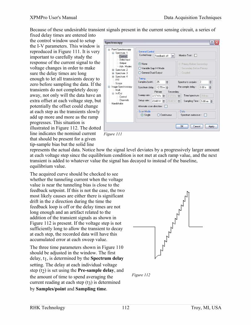
XPMPro User's Manual Data Acquisition Techniques
Because of these undesirable transient signals present in the current sensing circuit, a series of fixed delay times are entered into the control window used to setup the I-V parameters. This window is reproduced in Figure 111. It is very important to carefully study the response of the current signal to the voltage changes in order to make sure the delay times are long enough to let all transients decay to zero before sampling the data. If the transients do not completely decay away, not only will the data have an extra offset at each voltage step, but potentially the offset could change at each step as the transients slowly add up more and more as the ramp progresses. This situation is illustrated in Figure 112. The dotted line indicates the nominal current that should be present for a given tip-sample bias but the solid line represents the actual data. Notice how the signal level deviates by a progressively larger amount at each voltage step since the equilibrium condition is not met at each ramp value, and the next transient is added to whatever value the signal has decayed to instead of the baseline, equilibrium value. The acquired curve should be checked to see whether the tunneling current when the voltage value is near the tunneling bias is close to the feedback setpoint. If this is not the case, the two most likely causes are either there is significant drift in the z direction during the time the feedback loop is off or the delay times are not long enough and an artifact related to the addition of the transient signals as shown in Figure 112 is present. If the voltage step is not sufficiently long to allow the transient to decay at each step, the recorded data will have this accumulated error at each sweep value.The three time parameters shown in Figure 110 should be adjusted in the window. The first delay, t1, is determined by the Spectrum delay setting. The delay at each individual voltage step (t2) is set using the Pre-sample delay, and the amount of time to spend averaging the current reading at each step (t3) is determined by Samples/point and Sampling time.
RHK Technology 112 Troy, MI, USA
Figure 111
Figure 112
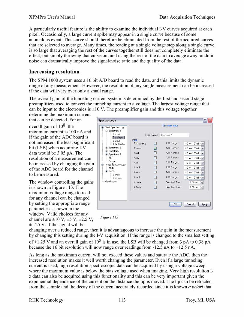
XPMPro User's Manual Data Acquisition Techniques
A particularly useful feature is the ability to examine the individual I-V curves acquired at each pixel. Occasionally, a large current spike may appear in a single curve because of some anomalous event. This curve should therefore be eliminated from the rest of the acquired curves that are selected to average. Many times, the reading at a single voltage step along a single curve is so large that averaging the rest of the curves together still does not completely eliminate the effect, but simply throwing that curve out and using the rest of the data to average away random noise can dramatically improve the signal/noise ratio and the quality of the data.
Increasing resolutionThe SPM 1000 system uses a 16 bit A/D board to read the data, and this limits the dynamic range of any measurement. However, the resolution of any single measurement can be increased if the data will vary over only a small range.The overall gain of the tunneling current system is determined by the first and second stage preamplifiers used to convert the tunneling current to a voltage. The largest voltage range that can be input to the electronics is ±10 V. The preamplifier gain and this voltage together determine the maximum current that can be detected. For an overall gain of 108, the maximum current is 100 nA and if the gain of the ADC board is not increased, the least significant bit (LSB) when acquiring I-V data would be 3.05 pA. The resolution of a measurement can be increased by changing the gain of the ADC board for the channel to be measured. The window controlling the gains is shown in Figure 113. The maximum voltage range to read for any channel can be changed by setting the appropriate range parameter as shown in the window. Valid choices for any channel are ±10 V, ±5 V, ±2.5 V, ±1.25 V. If the signal will be changing over a reduced range, then it is advantageous to increase the gain in the measurement by changing this setting during the I-V acquisition. If the range is changed to the smallest setting of ±1.25 V and an overall gain of 108 is in use, the LSB will be changed from 3 pA to 0.38 pA because the 16 bit resolution will now range over readings from -12.5 nA to +12.5 nA.As long as the maximum current will not exceed these values and saturate the ADC, then the increased resolution makes it well worth changing the parameter. Even if a large tunneling current is used, high resolution spectroscopic data can be acquired by using a voltage sweep where the maximum value is below the bias voltage used when imaging. Very high resolution I-z data can also be acquired using this functionality and this can be very important given the exponential dependence of the current on the distance the tip is moved. The tip can be retracted from the sample and the decay of the current accurately recorded since it is known a priori that
RHK Technology 113 Troy, MI, USA
Figure 113
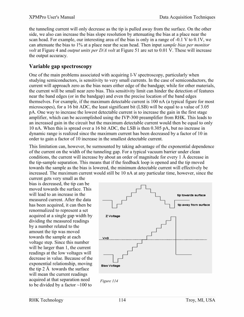
XPMPro User's Manual Data Acquisition Techniques
the tunneling current will only decrease as the tip is pulled away from the surface. On the other side, we also can increase the bias slope resolution by attenuating the bias at a place near the scan head. For example, our interesting area of the bias is only in a range of -0.1 V to 0.1V, we can attenuate the bias to 1% at a place near the scan head. Then input sample bias per monitor volt at Figure 4 and output units per D/A volt at Figure 51 are set to 0.01 V. These will increase the output accuracy.
Variable gap spectroscopyOne of the main problems associated with acquiring I-V spectroscopy, particularly when studying semiconductors, is sensitivity to very small currents. In the case of semiconductors, the current will approach zero as the bias nears either edge of the bandgap; while for other materials, the current will be small near zero bias. This sensitivity limit can hinder the detection of features near the band edges (or in the bandgap) and even the precise location of the band edges themselves. For example, if the maximum detectable current is 100 nA (a typical figure for most microscopes), for a 16 bit ADC, the least significant bit (LSB) will be equal to a value of 3.05 pA. One way to increase the lowest detectable current is to increase the gain in the first stage amplifier, which can be accomplished using the IVP-300 preamplifier from RHK. This leads to an increased gain in the circuit but the maximum detectable current would then be equal to only 10 nA. When this is spread over a 16 bit ADC, the LSB is then 0.305 pA, but no increase in dynamic range is realized since the maximum current has been decreased by a factor of 10 in order to gain a factor of 10 increase in the smallest detectable current.This limitation can, however, be surmounted by taking advantage of the exponential dependence of the current on the width of the tunneling gap. For a typical vacuum barrier under clean conditions, the current will increase by about an order of magnitude for every 1 Å decrease in the tip-sample separation. This means that if the feedback loop is opened and the tip moved towards the sample as the bias is lowered, the minimum detectable current will effectively be increased. The maximum current would still be 10 nA at any particular time, however, since the current gets very small as the bias is decreased, the tip can be moved towards the surface. This will lead to an increase in the measured current. After the data has been acquired, it can then be renormalized to represent a set acquired at a single gap width by dividing the measured readings by a number related to the amount the tip was moved towards the sample at each voltage step. Since this number will be larger than 1, the current readings at the low voltages will decrease in value. Because of the exponential relationship, moving the tip 2 Å towards the surface will mean the current readings acquired at that separation need to be divided by a factor ~100 to
RHK Technology 114 Troy, MI, USA
Figure 114
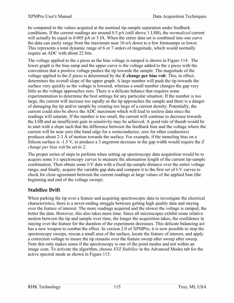
XPMPro User's Manual Data Acquisition Techniques
be compared to the values acquired at the nominal tip-sample separation under feedback conditions. If the current readings are around 0.5 pA (still above 1 LSB), the normalized current will actually be equal to 0.005 pA or 5 fA. When the entire data set is combined into one curve the data can easily range from the maximum near 10 nA down to a few femtoamps or lower. This represents a total dynamic range of 6 or 7 orders of magnitude, which would normally require an ADC with about 22 bits.The voltage applied to the z piezo as the bias voltage is ramped is shown in Figure 114. The lower graph is the bias ramp and the upper curve is the voltage added to the z piezo with the convention that a positive voltage pushes the tip towards the sample. The magnitude of the voltage applied to the Z piezo is determined by the Z change per bias volt. This, in effect, determines the overall slope of the upper graph. A large number will push the tip towards the surface very quickly as the voltage is lowered, whereas a small number changes the gap very little as the voltage approaches zero. There is a delicate balance that requires some experimentation to determine the best settings for any particular situation. If the number is too large, the current will increase too rapidly as the tip approaches the sample and there is a danger of damaging the tip and/or sample by creating too large of a current density. Potentially, the current could also be above the ADC maximum which will lead to useless data since the readings will saturate. If the number is too small, the current will continue to decrease towards the LSB and an insufficient gain in sensitivity may be achieved. A good rule of thumb would be to start with a slope such that the difference between the feedback bias and the voltage where the current will be near zero (the band edge for a semiconductor, zero for other conductors) produces about 2-3 Å of motion towards the surface. For example, if the tunneling bias on a Silicon surface is -1.5 V, to produce a 3 angstrom decrease in the gap width would require the Z change per bias volt be set to 2.The proper series of steps to perform when setting up spectroscopy data acquisition would be to acquire some I-z spectroscopy curves to measure the attenuation length of the current tip-sample combination. Then obtain some I-V data with a fixed tip-sample distance over the entire voltage range, and finally, acquire the variable gap data and compare it to the first set of I-V curves to check for close agreement between the current readings at large values of the applied bias (the beginning and end of the voltage sweep).
Stabilize DriftWhen parking the tip over a feature and acquiring spectroscopic data to investigate the electrical characteristics, there is a never-ending struggle between getting high quality data and staying over the feature of interest. The more readings acquired and the slower the voltage is ramped, the better the data. However, this also takes more time. Since all microscopes exhibit some relative motion between the tip and sample over time, the longer the acquisition takes, the confidence in staying over the feature for the duration of the experiment decreases. This delicate balancing act has a new weapon to combat the effect. In version 2.0 of XPMPro, it is now possible to stop the spectroscopy sweeps, rescan a small area of the surface, locate the feature of interest, and apply a correction voltage to insure the tip remains over the feature sweep after sweep after sweep. Note this only makes sense if the spectroscopy is one of the point modes and not within an image scan. To activate the algorithm, choose XYZ Stabilize in the Advanced Modes tab for the active spectral mode as shown in Figure 115.
RHK Technology 115 Troy, MI, USA
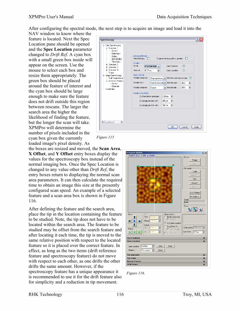
XPMPro User's Manual Data Acquisition Techniques
After configuring the spectral mode, the next step is to acquire an image and load it into the NAV window to know where the feature is located. Next the Spec Location pane should be opened and the Spec Location parameter changed to Drift Ref. A cyan box with a small green box inside will appear on the screen. Use the mouse to select each box and resize them appropriately. The green box should be placed around the feature of interest and the cyan box should be large enough to make sure the feature does not drift outside this region between rescans. The larger the search area the higher the likelihood of finding the feature, but the longer the scan will take. XPMPro will determine the number of pixels included in the cyan box given the currently loaded image's pixel density. As the boxes are resized and moved, the Scan Area, X Offset, and Y Offset entry boxes display the values for the spectroscopy box instead of the normal imaging box. Once the Spec Location is changed to any value other than Drift Ref, the entry boxes return to displaying the normal scan area parameters. It can then calculate the required time to obtain an image this size at the presently configured scan speed. An example of a selected feature and a scan area box is shown in Figure116.
After defining the feature and the search area, place the tip in the location containing the feature to be studied. Note, the tip does not have to be located within the search area. The feature to be studied may be offset from the search feature and after locating it each time, the tip is moved to the same relative position with respect to the located feature so it is placed over the correct feature. In effect, as long as the two items (drift reference feature and spectroscopy feature) do not move with respect to each other, as one drifts the other drifts the same amount. However, if the spectroscopy feature has a unique appearance it is recommended to use it for the drift feature also for simplicity and a reduction in tip movement.
RHK Technology 116 Troy, MI, USA
Figure 115
Figure 116.
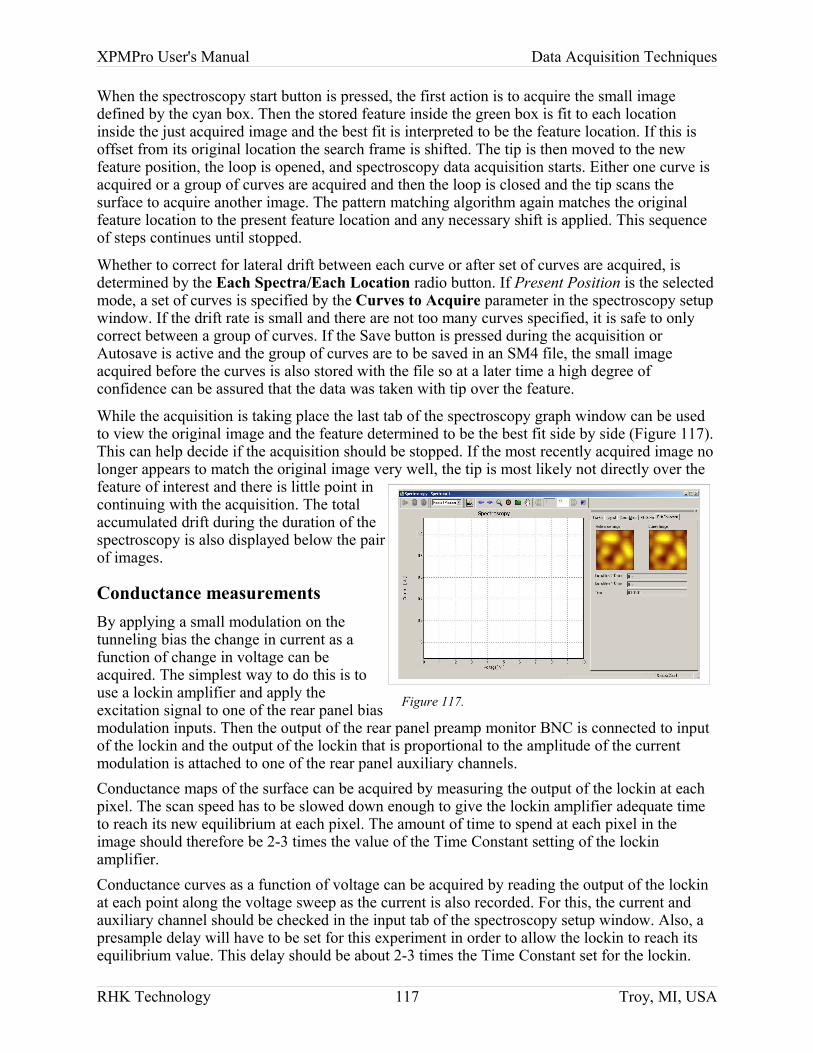
XPMPro User's Manual Data Acquisition Techniques
When the spectroscopy start button is pressed, the first action is to acquire the small image defined by the cyan box. Then the stored feature inside the green box is fit to each location inside the just acquired image and the best fit is interpreted to be the feature location. If this is offset from its original location the search frame is shifted. The tip is then moved to the new feature position, the loop is opened, and spectroscopy data acquisition starts. Either one curve is acquired or a group of curves are acquired and then the loop is closed and the tip scans the surface to acquire another image. The pattern matching algorithm again matches the original feature location to the present feature location and any necessary shift is applied. This sequence of steps continues until stopped.
Whether to correct for lateral drift between each curve or after set of curves are acquired, is determined by the Each Spectra/Each Location radio button. If Present Position is the selected mode, a set of curves is specified by the Curves to Acquire parameter in the spectroscopy setup window. If the drift rate is small and there are not too many curves specified, it is safe to only correct between a group of curves. If the Save button is pressed during the acquisition or Autosave is active and the group of curves are to be saved in an SM4 file, the small image acquired before the curves is also stored with the file so at a later time a high degree of confidence can be assured that the data was taken with tip over the feature.
While the acquisition is taking place the last tab of the spectroscopy graph window can be used to view the original image and the feature determined to be the best fit side by side (Figure 117). This can help decide if the acquisition should be stopped. If the most recently acquired image no longer appears to match the original image very well, the tip is most likely not directly over the feature of interest and there is little point in continuing with the acquisition. The total accumulated drift during the duration of the spectroscopy is also displayed below the pair of images.
Conductance measurementsBy applying a small modulation on the tunneling bias the change in current as a function of change in voltage can be acquired. The simplest way to do this is to use a lockin amplifier and apply the excitation signal to one of the rear panel bias modulation inputs. Then the output of the rear panel preamp monitor BNC is connected to input of the lockin and the output of the lockin that is proportional to the amplitude of the current modulation is attached to one of the rear panel auxiliary channels.Conductance maps of the surface can be acquired by measuring the output of the lockin at each pixel. The scan speed has to be slowed down enough to give the lockin amplifier adequate time to reach its new equilibrium at each pixel. The amount of time to spend at each pixel in the image should therefore be 2-3 times the value of the Time Constant setting of the lockin amplifier.Conductance curves as a function of voltage can be acquired by reading the output of the lockin at each point along the voltage sweep as the current is also recorded. For this, the current and auxiliary channel should be checked in the input tab of the spectroscopy setup window. Also, a presample delay will have to be set for this experiment in order to allow the lockin to reach its equilibrium value. This delay should be about 2-3 times the Time Constant set for the lockin.
RHK Technology 117 Troy, MI, USA
Figure 117.
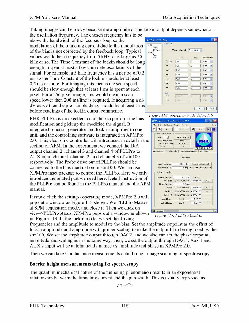
XPMPro User's Manual Data Acquisition Techniques
Taking images can be tricky because the amplitude of the lockin output depends somewhat on the oscillation frequency. The chosen frequency has to be above the bandwidth of the feedback loop so the modulation of the tunneling current due to the modulation of the bias is not corrected by the feedback loop. Typical values would be a frequency from 5 kHz to as large as 20 kHz or so. The Time Constant of the lockin should be long enough to span at least a few complete oscillations of the signal. For example, a 5 kHz frequency has a period of 0.2 ms so the Time Constant of the lockin should be at least 0.5 ms or more. For imaging this means the scan speed should be slow enough that at least 1 ms is spent at each pixel. For a 256 pixel image, this would mean a scan speed lower then 200 ms/line is required. If acquiring a dI/dV curve then the pre-sample delay should be at least 1 ms before readings of the lockin output commence. RHK PLLPro is an excellent candidate to perform the bias modification and pick up the modified the signal. It integrated function generator and lock-in amplifier to one unit, and the controlling software is integrated in XPMPro 2.0. This electronic controller will introduced in detail in the section of AFM. In the experiment, we connect the D/A output channel 2 , channel 3 and channel 4 of PLLPro to AUX input channel, channel 2, and channel 3 of stm100 respectively. The Probe drive out of PLLPro should be connected to the bias modulation in stm100. We can use XPMPro inset package to control the PLLPro. Here we only introduce the related part we need here. Detail instruction of the PLLPro can be found in the PLLPro manual and the AFM manual.First,we click the setting->operating mode, XPMPro 2.0 will pop out a window as Figure 118 shown. We PLLPro Master at SPM acquisition mode, and close it. Then we click on view->PLLPro status, XPMPro pops out a window as shown in Figure 119. In the lockin mode, we set the driving frequencies and the amplitude to modulate the bias. Set the amplitude setpoint as the offset of lockin amplitude and amplitude with proper scaling to make the output fit to be digitized by the stm100. We set the amplitude output through DAC2, and we also can set the phase setpoint, amplitude and scaling as in the same way; then, we set the output through DAC3. Aux 1 and AUX 2 input will be automatically named as amplitude and phase in XPMPro 2.0.Then we can take Conductance measurements data through image scanning or spectroscopy.
Barrier height measurements using I-z spectroscopy
The quantum mechanical nature of the tunneling phenomenon results in an exponential relationship between the tunneling current and the gap width. This is usually expressed as
I ∝ e−2kz
RHK Technology 118 Troy, MI, USA
Figure 118: operation mode define tab
Figure 119: PLLPro Control
XPMPro User's Manual Data Acquisition Techniques
where k is a constant that depends on some physical constants as well as the mean barrier height of the gap and z is the tunneling gap distance. The value of k, and hence the barrier height itself can be determined by obtaining spectroscopy data. In this routine, the feedback loop is opened and the tip is moved away from the surface while recording the current at each step. This data will exhibit an exponential decay equal to 2k. This data usually does not have the transient signals present compared to the I-V data because there is little reason for coupling between the current and the z piezo position given a good scan head design where the two signals are isolated from each other. It is usually a good idea to still use a small pre-sample delay in the spectroscopy window to allow the piezo tube to settle for a small amount of time after the tip has moved, but large peaks as seen in the I-V section above are rarely seen.The slope of an I-z curve when plotted on a linear (z)-logarithmic (I) scale can be determined by a simple fitting routine and this would be used to calculate the barrier height. Once the slope, m, is known; the barrier height is calculated using this equation
= m1.025
2
Various features on the surface such as contamination or defects can create a local variation in the barrier height and this can be seen by acquiring I-z curves in two distinct regions and comparing the value of Φ derived from the two sets of data. Additionally, as described above this data is also used to determine the attenuation length that is needed for proper normalization of variable gap I-V spectroscopy data. The correct value can be ascertained by simply looking at a plot of the I-z data and noting the ratio of two current readings that are separated by a given distance. Select any current value and then find the value that is e-2 times smaller.
Barrier height measurements using a lockin amplifier
As discussed in the previous section, features on the surface can change the local work function, and this can be measured with a STM. A direct correlation between the topographic structure and the work function can then be obtained. The best method to acquire this type of data is to apply a small oscillation to the z piezo so the tip-sample distance oscillates a small amount. If the modulation frequency is high enough that the feedback loop cannot compensate for it, then there will be an oscillatory signal superimposed on the tunneling current at the same frequency. This can be monitored by a lock-in amplifier and the signal from the lock-in would then be proportional to the local work function. If an image is formed of this signal along with a topographic image, common features in both images can be correlated.Some additional cables are required to connect the lock-in amplifier properly. The oscillation signal out of the lock-in amplifier should be connected to Z modulation input #2, and the current monitor output on the rear panel of the SPM 100 should be connected to the input of the lock-in. The amplitude output of the lock-in should then be connected to one of the rear panel auxiliary inputs. To simultaneously acquire the topographic image along with the output of the lock-in, the auxiliary channel connected to the lock-in output should be turned ON in the Input tab contained in the Settings/Scan window. For a more meaningful display of the barrier height image, the label of the auxiliary channel being used could be renamed to something more descriptive like “barrier height” or “amplitude”. This is done in the Settings/Operating modes/Define tab.While the tip is scanned, the two input channels will each be sampled for an equal amount of
RHK Technology 119 Troy, MI, USA
XPMPro User's Manual Data Acquisition Techniques
time before the tip is moved to the next pixel. Both the topography and lock-in signal should also be saved in the data files. The signal stored from the lock-in output then has to be converted from Vout of the lock-in into eV of mean barrier height. The derivation of this scaling factor is presented below.From basic tunneling theory, we know the current is an exponential function with the form
I ∝ e−2kz
where k is constant that includes the barrier height and z is the tunneling gap distance. A typical value gives a decay of about an order of magnitude in current for every 1 Angstrom change in the gap distance.If we modulate the gap distance by a small amount δz using a sinusoidal function, then the gap width will have the form
z=z0 z cos t
and the tunneling current then has this formI ∝e−2z 0 zcos t
which can be rewritten asI ∝e−2z 0∗e−2 zcos t
If the modulation frequency is well above the bandwidth of the feedback loop, the first part of the expression is simply the normal feedback tunneling current, I0. If the modulation amplitude is small, then the exponential can be expanded via Taylor’s series to be
I ∝I 01−2 z cos t
A lock-in amplifier operates by taking the input signal and detecting the portion of it that is at the same frequency as the output frequency (which in this case is being used to modulate the height). Most lock-in amplifiers will output a signal that is equal to the rms value of the cos term. For this situation, the amplitude of the signal is
−I 0∗2 z
This rms introduces an additional square root of 2 into the expression so the output signal will be related to the modulated current detected by the lock-in amplifier by
−I 0∗2 z 12
Solving for k gives the expression
=−I lockin
I 0∗ z 1 /2
From a quantum mechanical derivation of tunneling, k will involve some constants related to the electron and the mean barrier height Φ which becomes
2=1.025 substituting this expression into the derivation of k above yields
RHK Technology 120 Troy, MI, USA
XPMPro User's Manual Data Acquisition Techniques
= I lockin2 I 0 z 1.025
2
When the modulation is set on most lock-in amplifiers, the voltage selected is actually the rms voltage applied to the z modulation, and this means the δz amplitude can be expressed as the rms value of the modulation which is
z=z lockin
2
If we substitute this into the above expression, the (rather confusing) square roots cancel and the final expression is
= I lockin
I 0 z rms1.0252
Measurement parameters
For some starting numbers, set the modulation voltage on the lock-in to 100 mV which should correspond to shaking the tip a tenth of an angstrom. As the signal is increased, some ripple on the tunneling current should appear when displayed on an oscilloscope. A frequency of a few kHz is a good starting point. When the oscillation amplitude is increased, the output signal of the lock-in amplifier should also increase since the amplitude of the current modulation also increases.It is a good idea to make a quick calculation while not scanning to see if the value for the barrier height makes sense given the tunneling conditions. The conversion from the output voltage of the lock-in amplifier into tunneling current should be whatever gain is in the system. If an IVP 200 is used which provides 108 gain and the IVP-PGA is set to x10, the overall gain is 109 V/A so 1 V output from the lock-in corresponds to 1 nA current. If the output signal from the lock-in amplifier is 10 mV (for example), then the resulting modulation on the current due to the z dither is 10 pA (0.01 V / 1 V/nA is 0.01 nA which is 10 pA).To calculate the local change over certain features, average the voltage output from the lock-in at pixels that are over the feature to obtain one value. Then convert this to equivalent current as described previously and this can then be converted to the mean barrier height using the final equation above. This should be compared to the value obtained by averaging a large area over the normal surface far from any defects.
Input/Output line-by-line imagingA particularly useful feature of XPMPro is the in/out image spectroscopy mode. Imaging conditions can be changed on an image-by-image or line-by-line basis. There are a plethora of experiments that can be performed using this capability.The main use for this is to measure friction forces using an AFM. The normal force can be changed every line and the slow scan axis is disabled so the same area of the surface is scanned repeatedly. If lateral force data is acquired, then the acquired image will be a record of the lateral force as the normal force increases.However, there are many other potentially useful experiments that can be done. One example is
RHK Technology 121 Troy, MI, USA
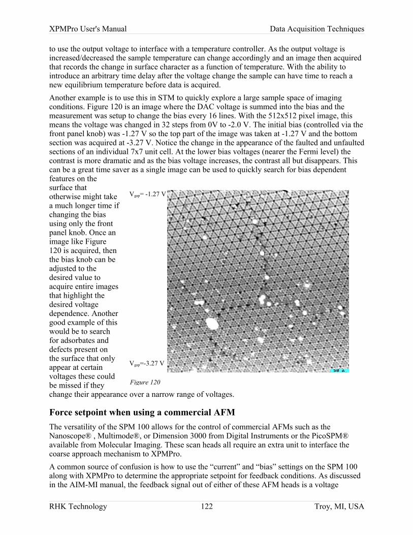
XPMPro User's Manual Data Acquisition Techniques
to use the output voltage to interface with a temperature controller. As the output voltage is increased/decreased the sample temperature can change accordingly and an image then acquired that records the change in surface character as a function of temperature. With the ability to introduce an arbitrary time delay after the voltage change the sample can have time to reach a new equilibrium temperature before data is acquired.Another example is to use this in STM to quickly explore a large sample space of imaging conditions. Figure 120 is an image where the DAC voltage is summed into the bias and the measurement was setup to change the bias every 16 lines. With the 512x512 pixel image, this means the voltage was changed in 32 steps from 0V to -2.0 V. The initial bias (controlled via the front panel knob) was -1.27 V so the top part of the image was taken at -1.27 V and the bottom section was acquired at -3.27 V. Notice the change in the appearance of the faulted and unfaulted sections of an individual 7x7 unit cell. At the lower bias voltages (nearer the Fermi level) the contrast is more dramatic and as the bias voltage increases, the contrast all but disappears. This can be a great time saver as a single image can be used to quickly search for bias dependent features on the surface that otherwise might take a much longer time if changing the bias using only the front panel knob. Once an image like Figure120 is acquired, then the bias knob can be adjusted to the desired value to acquire entire images that highlight the desired voltage dependence. Another good example of this would be to search for adsorbates and defects present on the surface that only appear at certain voltages these could be missed if they change their appearance over a narrow range of voltages.
Force setpoint when using a commercial AFMThe versatility of the SPM 100 allows for the control of commercial AFMs such as the Nanoscope® , Multimode®, or Dimension 3000 from Digital Instruments or the PicoSPM® available from Molecular Imaging. These scan heads all require an extra unit to interface the coarse approach mechanism to XPMPro.A common source of confusion is how to use the “current” and “bias” settings on the SPM 100 along with XPMPro to determine the appropriate setpoint for feedback conditions. As discussed in the AIM-MI manual, the feedback signal out of either of these AFM heads is a voltage
RHK Technology 122 Troy, MI, USA
Figure 120
Vgap= -1.27 V
Vgap=-3.27 V
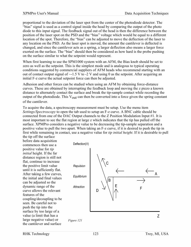
XPMPro User's Manual Data Acquisition Techniques
proportional to the deviation of the laser spot from the center of the photodiode detector. The “bias” signal is used as a control signal inside the head by comparing the output of the photo diode to this input signal. The feedback signal out of the head is then the difference between the position of the laser spot on the PSD and the “bias” voltage which would be equal to a different location of the spot. Therefore, the “bias” can be adjusted to move the deflection of the laser to any location on the PSD. As the laser spot is moved, the amount the cantilever is deflected is changed, and since the cantilever acts as a spring, a larger deflection also means a larger force exerted on the surface. The “bias” should then be considered as how hard is the probe pushing on the surface similar to what the setpoint would represent.When first learning to use the SPM1000 system with an AFM, the Bias knob should be set to zero as well as the setpoint. This is the simplest mode and is analogous to typical operating conditions suggested by commercial suppliers of AFM heads who recommend starting with an out of contact output signal of ~-1.5 V to -2 V and using 0 as the setpoint. After acquiring an initial F-z curve the actual setpoint force can then be adjusted.Adhesion and other forces can be studied when using an AFM by obtaining force-distance curves. These are obtained by interrupting the feedback loop and moving the z piezo a known distance to alternately contact the surface and break the tip-sample contact while recording the output of the photodiode. This Vout can then be converted into a force given the spring constant of the cantilever. To acquire the data, a spectroscopy measurement must be setup. Use the menu item Settings/Spectroscopy to open the tab used to setup an F-z curve. A BNC cable should be connected from one of the DAC Output channels to the Z Position Modulation Input #1. It is most important to see the flat region at large z which indicates that the tip has pulled off the surface. XPMPro considers a negative value to be decreasing the tip-sample separation and a positive value to pull the two apart. When taking an F-z curve, if it is desired to push the tip in first while remaining in contact, use a negative value for tip initial height. If it is desirable to pull the tip off the surface before data acquisition commences then use a positive value for tip initial height. If the far distance region is still not flat, continue to increase the positive limit value until it is sufficiently flat. After taking a few curves, the initial and final values can be adjusted so the dynamic range of the curve allows the relevant features of the coupling/decoupling to be seen. Be careful not to push the tip into the surface by too large of a value (a limit that has a large negative value) or the cantilever and surface
RHK Technology 123 Troy, MI, USA
Figure 121
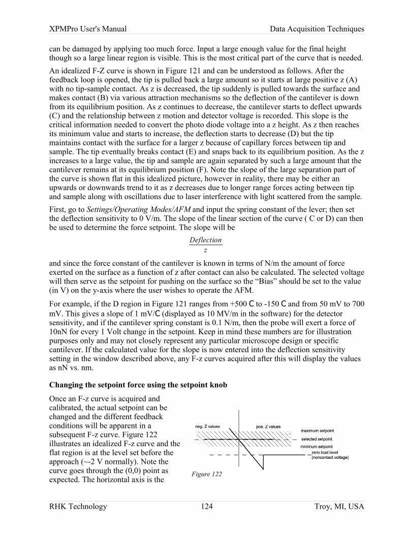
XPMPro User's Manual Data Acquisition Techniques
can be damaged by applying too much force. Input a large enough value for the final height though so a large linear region is visible. This is the most critical part of the curve that is needed.An idealized F-Z curve is shown in Figure 121 and can be understood as follows. After the feedback loop is opened, the tip is pulled back a large amount so it starts at large positive z (A) with no tip-sample contact. As z is decreased, the tip suddenly is pulled towards the surface and makes contact (B) via various attraction mechanisms so the deflection of the cantilever is down from its equilibrium position. As z continues to decrease, the cantilever starts to deflect upwards (C) and the relationship between z motion and detector voltage is recorded. This slope is the critical information needed to convert the photo diode voltage into a z height. As z then reaches its minimum value and starts to increase, the deflection starts to decrease (D) but the tip maintains contact with the surface for a larger z because of capillary forces between tip and sample. The tip eventually breaks contact (E) and snaps back to its equilibrium position. As the z increases to a large value, the tip and sample are again separated by such a large amount that the cantilever remains at its equilibrium position (F). Note the slope of the large separation part of the curve is shown flat in this idealized picture, however in reality, there may be either an upwards or downwards trend to it as z decreases due to longer range forces acting between tip and sample along with oscillations due to laser interference with light scattered from the sample.First, go to Settings/Operating Modes/AFM and input the spring constant of the lever; then set the deflection sensitivity to 0 V/m. The slope of the linear section of the curve ( C or D) can then be used to determine the force setpoint. The slope will be
Deflectionz
and since the force constant of the cantilever is known in terms of N/m the amount of force exerted on the surface as a function of z after contact can also be calculated. The selected voltage will then serve as the setpoint for pushing on the surface so the “Bias” should be set to the value (in V) on the y-axis where the user wishes to operate the AFM.
For example, if the D region in Figure 121 ranges from +500 C to -150 C and from 50 mV to 700 mV. This gives a slope of 1 mV/C (displayed as 10 MV/m in the software) for the detector sensitivity, and if the cantilever spring constant is 0.1 N/m, then the probe will exert a force of 10nN for every 1 Volt change in the setpoint. Keep in mind these numbers are for illustration purposes only and may not closely represent any particular microscope design or specific cantilever. If the calculated value for the slope is now entered into the deflection sensitivity setting in the window described above, any F-z curves acquired after this will display the values as nN vs. nm.
Changing the setpoint force using the setpoint knob
Once an F-z curve is acquired and calibrated, the actual setpoint can be changed and the different feedback conditions will be apparent in a subsequent F-z curve. Figure 122 illustrates an idealized F-z curve and the flat region is at the level set before the approach (~-2 V normally). Note the curve goes through the (0,0) point as expected. The horizontal axis is the
RHK Technology 124 Troy, MI, USA
Figure 122
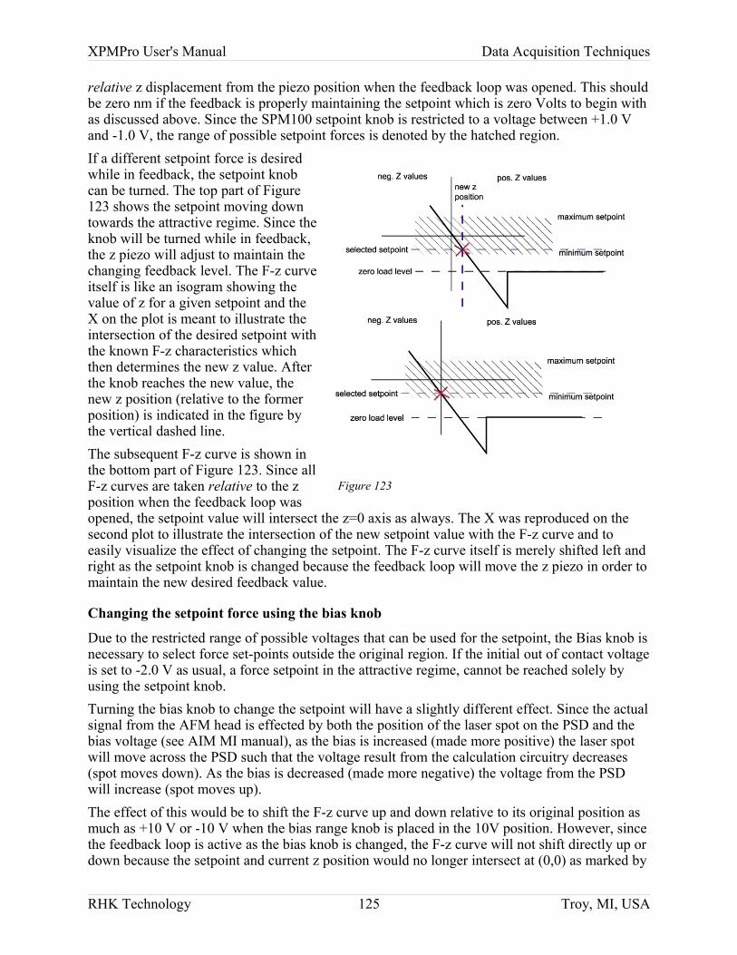
XPMPro User's Manual Data Acquisition Techniques
relative z displacement from the piezo position when the feedback loop was opened. This should be zero nm if the feedback is properly maintaining the setpoint which is zero Volts to begin with as discussed above. Since the SPM100 setpoint knob is restricted to a voltage between +1.0 V and -1.0 V, the range of possible setpoint forces is denoted by the hatched region.If a different setpoint force is desired while in feedback, the setpoint knob can be turned. The top part of Figure123 shows the setpoint moving down towards the attractive regime. Since the knob will be turned while in feedback, the z piezo will adjust to maintain the changing feedback level. The F-z curve itself is like an isogram showing the value of z for a given setpoint and the X on the plot is meant to illustrate the intersection of the desired setpoint with the known F-z characteristics which then determines the new z value. After the knob reaches the new value, the new z position (relative to the former position) is indicated in the figure by the vertical dashed line. The subsequent F-z curve is shown in the bottom part of Figure 123. Since all F-z curves are taken relative to the z position when the feedback loop was opened, the setpoint value will intersect the z=0 axis as always. The X was reproduced on the second plot to illustrate the intersection of the new setpoint value with the F-z curve and to easily visualize the effect of changing the setpoint. The F-z curve itself is merely shifted left and right as the setpoint knob is changed because the feedback loop will move the z piezo in order to maintain the new desired feedback value.
Changing the setpoint force using the bias knob
Due to the restricted range of possible voltages that can be used for the setpoint, the Bias knob is necessary to select force set-points outside the original region. If the initial out of contact voltage is set to -2.0 V as usual, a force setpoint in the attractive regime, cannot be reached solely by using the setpoint knob.Turning the bias knob to change the setpoint will have a slightly different effect. Since the actual signal from the AFM head is effected by both the position of the laser spot on the PSD and the bias voltage (see AIM MI manual), as the bias is increased (made more positive) the laser spot will move across the PSD such that the voltage result from the calculation circuitry decreases (spot moves down). As the bias is decreased (made more negative) the voltage from the PSD will increase (spot moves up).The effect of this would be to shift the F-z curve up and down relative to its original position as much as +10 V or -10 V when the bias range knob is placed in the 10V position. However, since the feedback loop is active as the bias knob is changed, the F-z curve will not shift directly up or down because the setpoint and current z position would no longer intersect at (0,0) as marked by
RHK Technology 125 Troy, MI, USA
Figure 123
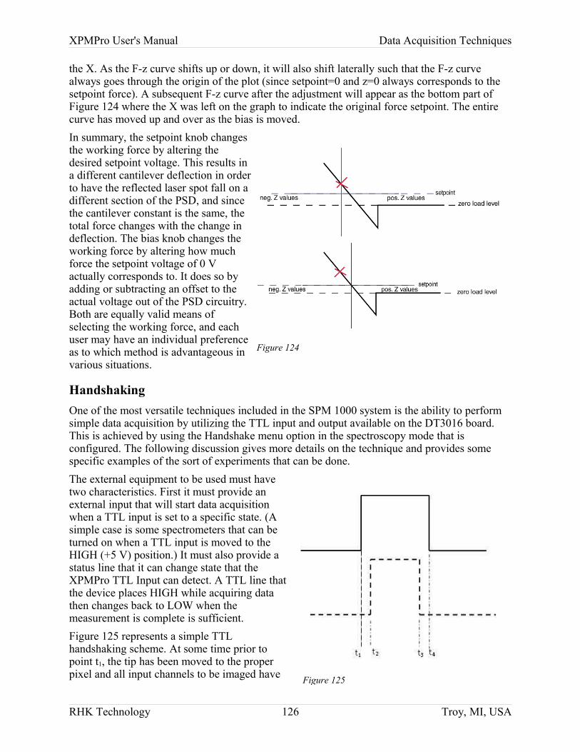
XPMPro User's Manual Data Acquisition Techniques
the X. As the F-z curve shifts up or down, it will also shift laterally such that the F-z curve always goes through the origin of the plot (since setpoint=0 and z=0 always corresponds to the setpoint force). A subsequent F-z curve after the adjustment will appear as the bottom part of Figure 124 where the X was left on the graph to indicate the original force setpoint. The entire curve has moved up and over as the bias is moved.In summary, the setpoint knob changes the working force by altering the desired setpoint voltage. This results in a different cantilever deflection in order to have the reflected laser spot fall on a different section of the PSD, and since the cantilever constant is the same, the total force changes with the change in deflection. The bias knob changes the working force by altering how much force the setpoint voltage of 0 V actually corresponds to. It does so by adding or subtracting an offset to the actual voltage out of the PSD circuitry. Both are equally valid means of selecting the working force, and each user may have an individual preference as to which method is advantageous in various situations.
HandshakingOne of the most versatile techniques included in the SPM 1000 system is the ability to perform simple data acquisition by utilizing the TTL input and output available on the DT3016 board. This is achieved by using the Handshake menu option in the spectroscopy mode that is configured. The following discussion gives more details on the technique and provides some specific examples of the sort of experiments that can be done.The external equipment to be used must have two characteristics. First it must provide an external input that will start data acquisition when a TTL input is set to a specific state. (A simple case is some spectrometers that can be turned on when a TTL input is moved to the HIGH (+5 V) position.) It must also provide a status line that it can change state that the XPMPro TTL Input can detect. A TTL line that the device places HIGH while acquiring data then changes back to LOW when the measurement is complete is sufficient. Figure 125 represents a simple TTL handshaking scheme. At some time prior to point t1, the tip has been moved to the proper pixel and all input channels to be imaged have
RHK Technology 126 Troy, MI, USA
Figure 124
Figure 125
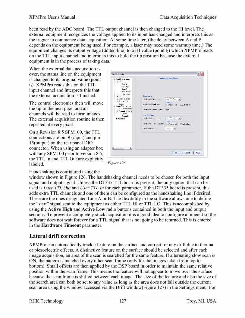
XPMPro User's Manual Data Acquisition Techniques
been read by the ADC board. The TTL output channel is then changed to the HI level. The external equipment recognizes the voltage applied to its input has changed and interprets this as the trigger to commence data acquisition. At some time later, (the delay between A and B depends on the equipment being used. For example, a laser may need some warmup time.) The equipment changes its output voltage (dotted line) to a HI value (point t2) which XPMPro reads on the TTL input channel and interprets this to hold the tip position because the external equipment is in the process of taking data.When the external data acquisition is over, the status line on the equipment is changed to its original value (point t3). XPMPro reads this on the TTL input channel and interprets this that the external acquisition is finished.The control electronics then will move the tip to the next pixel and all channels will be read to form images. The external acquisition routine is then repeated at every pixel.On a Revision 8.5 SPM100, the TTL connections are pin 9 (input) and pin 15(output) on the rear panel DIO connector. When using an adapter box with any SPM100 prior to version 8.5, the TTL In and TTL Out are explicitly labeled.Handshaking is configured using the window shown in Figure 126. The handshaking channel needs to be chosen for both the input signal and output signal. Unless the DT335 TTL board is present, the only option that can be used is User TTL Out and User TTL In for each parameter. If the DT335 board is present, this adds extra TTL channels and one of them can be configured as the handshaking line if desired. These are the ones designated Line A or B. The flexibility in the software allows one to define the “start” signal sent to the equipment as either TTL HI or TTL LO. This is accomplished by using the Active High and Active Low radio buttons contained in both the input and output sections. To prevent a completely stuck acquisition it is a good idea to configure a timeout so the software does not wait forever for a TTL signal that is not going to be returned. This is entered in the Hardware Timeout parameter.
Lateral drift correctionXPMPro can automatically track a feature on the surface and correct for any drift due to thermal or piezoelectric effects. A distinctive feature on the surface should be selected and after each image acquisition, an area of the scan is searched for the same feature. If alternating slow scan is ON, the pattern is matched every other scan frame (only for the images taken from top to bottom). Small offsets are then applied by the DSP board in order to maintain the same relative position within the scan frame. This means the feature will not appear to move over the surface because the scan frame is shifted between each image. The size of the feature and also the size of the search area can both be set to any value as long as the area does not fall outside the current scan area using the window accessed via the Drift window(Figure 127) in the Settings menu. For
RHK Technology 127 Troy, MI, USA
Figure 126
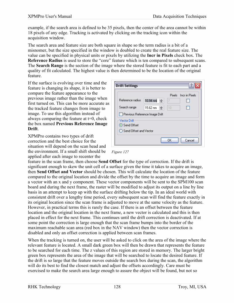
XPMPro User's Manual Data Acquisition Techniques
example, if the search area is defined to be 35 pixels, then the center of the area cannot be within 18 pixels of any edge. Tracking is activated by clicking on the tracking icon within the acquisition window.The search area and feature size are both square in shape so the term radius is a bit of a misnomer, but the size specified in the window is doubled to create the real feature size. The value can be specified in physical units or pixels by utilizing the Incr in Pixels check box. The Reference Radius is used to store the “core” feature which is ten compared to subsequent scans. The Search Range is the section of the image where the stored feature is fit to each part and a quality of fit calculated. The highest value is then determined to be the location of the original feature. If the surface is evolving over time and the feature is changing its shape, it is better to compare the feature appearance to the previous image rather than the image when first turned on. This can be more accurate as the tracked feature changes from image to image. To use this algorithm instead of always comparing the feature at t=0, check the box named Previous Reference Image Drift.XPMPro contains two types of drift correction and the best choice for the situation will depend on the scan head and the environment. If a small shift should be applied after each image to recenter the feature in the scan frame, then choose Send Offset for the type of correction. If the drift is significant enough to skew the unit cell of a surface given the time it takes to acquire an image, then Send Offset and Vector should be chosen. This will calculate the location of the feature compared to the original location and divide the offset by the time to acquire an image and form a vector with an x and y component. These vector components will be sent to the SPM100 scan board and during the next frame, the raster will be modified to adjust its output on a line by line basis in an attempt to keep up with the surface drifting below the tip. In an ideal world with consistent drift over a lengthy time period, every subsequent scan will find the feature exactly in its original location since the scan frame is adjusted to move at the same velocity as the feature. However, in practical terms this is rarely the case. If there is an offset between the feature location and the original location in the next frame, a new vector is calculated and this is then placed in effect for the next frame. This continues until the drift correction is deactivated. If at some point the correction is large enough that the scan frame bumps into the border of the maximum reachable scan area (red box in the NAV window) then the vector correction is disabled and only an offset correction is applied between scan frames.When the tracking is turned on, the user will be asked to click on the area of the image where the relevant feature is located. A small dark green box will then be drawn that represents the feature to be searched for each time. The z values of this region are stored in memory. The larger bright green box represents the area of the image that will be searched to locate the desired feature. If the drift is so large that the feature moves outside the search box during the scan, the algorithm will do its best to find the closest match and adjust the offsets accordingly. Care must be exercised to make the search area large enough to assure the object will be found, but not so
RHK Technology 128 Troy, MI, USA
Figure 127
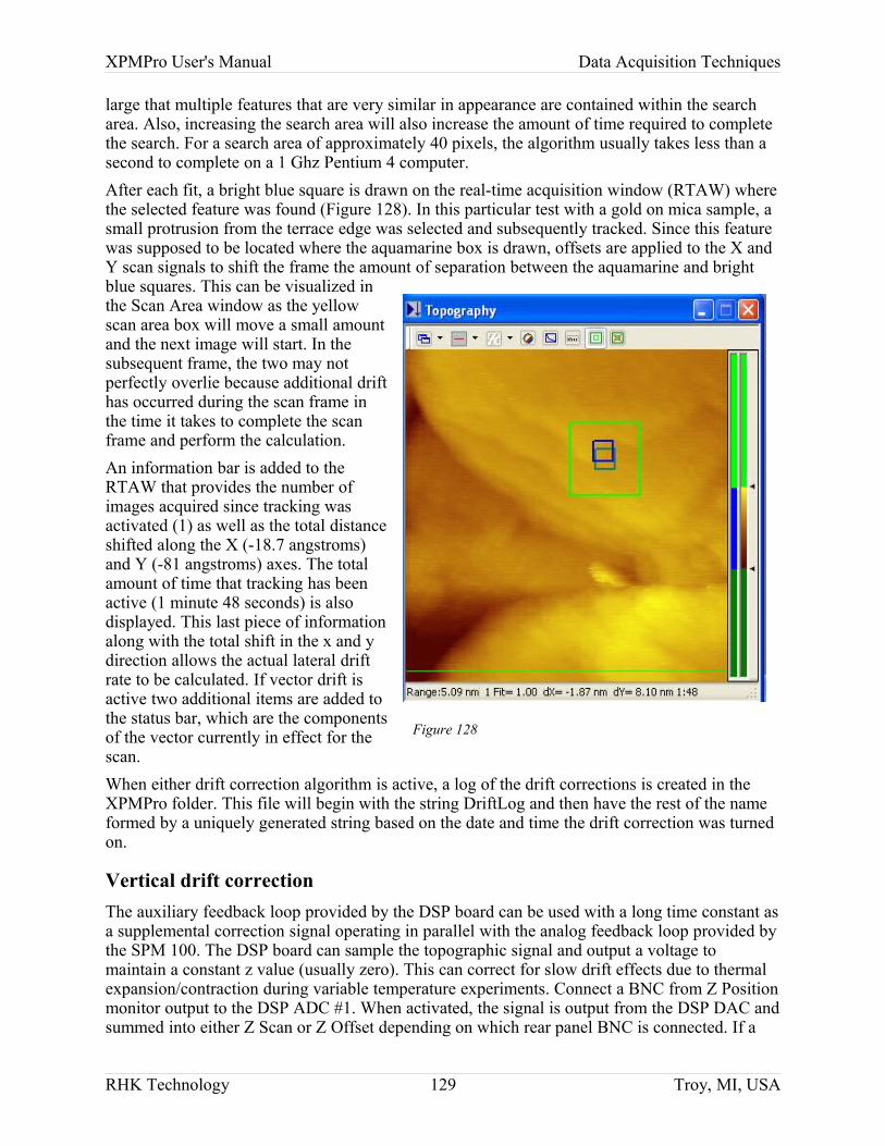
XPMPro User's Manual Data Acquisition Techniques
large that multiple features that are very similar in appearance are contained within the search area. Also, increasing the search area will also increase the amount of time required to complete the search. For a search area of approximately 40 pixels, the algorithm usually takes less than a second to complete on a 1 Ghz Pentium 4 computer.After each fit, a bright blue square is drawn on the real-time acquisition window (RTAW) where the selected feature was found (Figure 128). In this particular test with a gold on mica sample, a small protrusion from the terrace edge was selected and subsequently tracked. Since this feature was supposed to be located where the aquamarine box is drawn, offsets are applied to the X and Y scan signals to shift the frame the amount of separation between the aquamarine and bright blue squares. This can be visualized in the Scan Area window as the yellow scan area box will move a small amount and the next image will start. In the subsequent frame, the two may not perfectly overlie because additional drift has occurred during the scan frame in the time it takes to complete the scan frame and perform the calculation.An information bar is added to the RTAW that provides the number of images acquired since tracking was activated (1) as well as the total distance shifted along the X (-18.7 angstroms) and Y (-81 angstroms) axes. The total amount of time that tracking has been active (1 minute 48 seconds) is also displayed. This last piece of information along with the total shift in the x and y direction allows the actual lateral drift rate to be calculated. If vector drift is active two additional items are added to the status bar, which are the components of the vector currently in effect for the scan.When either drift correction algorithm is active, a log of the drift corrections is created in the XPMPro folder. This file will begin with the string DriftLog and then have the rest of the name formed by a uniquely generated string based on the date and time the drift correction was turned on.
Vertical drift correctionThe auxiliary feedback loop provided by the DSP board can be used with a long time constant as a supplemental correction signal operating in parallel with the analog feedback loop provided by the SPM 100. The DSP board can sample the topographic signal and output a voltage to maintain a constant z value (usually zero). This can correct for slow drift effects due to thermal expansion/contraction during variable temperature experiments. Connect a BNC from Z Position monitor output to the DSP ADC #1. When activated, the signal is output from the DSP DAC and summed into either Z Scan or Z Offset depending on which rear panel BNC is connected. If a
RHK Technology 129 Troy, MI, USA
Figure 128
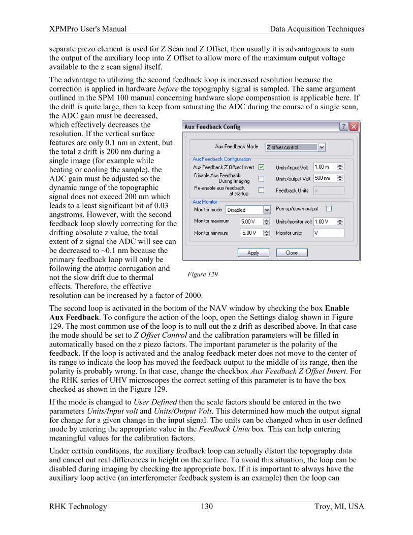
XPMPro User's Manual Data Acquisition Techniques
separate piezo element is used for Z Scan and Z Offset, then usually it is advantageous to sum the output of the auxiliary loop into Z Offset to allow more of the maximum output voltage available to the z scan signal itself. The advantage to utilizing the second feedback loop is increased resolution because the correction is applied in hardware before the topography signal is sampled. The same argument outlined in the SPM 100 manual concerning hardware slope compensation is applicable here. If the drift is quite large, then to keep from saturating the ADC during the course of a single scan, the ADC gain must be decreased, which effectively decreases the resolution. If the vertical surface features are only 0.1 nm in extent, but the total z drift is 200 nm during a single image (for example while heating or cooling the sample), the ADC gain must be adjusted so the dynamic range of the topographic signal does not exceed 200 nm which leads to a least significant bit of 0.03 angstroms. However, with the second feedback loop slowly correcting for the drifting absolute z value, the total extent of z signal the ADC will see can be decreased to ~0.1 nm because the primary feedback loop will only be following the atomic corrugation and not the slow drift due to thermal effects. Therefore, the effective resolution can be increased by a factor of 2000.The second loop is activated in the bottom of the NAV window by checking the box Enable Aux Feedback. To configure the action of the loop, open the Settings dialog shown in Figure129. The most common use of the loop is to null out the z drift as described above. In that case the mode should be set to Z Offset Control and the calibration parameters will be filled in automatically based on the z piezo factors. The important parameter is the polarity of the feedback. If the loop is activated and the analog feedback meter does not move to the center of its range to indicate the loop has moved the feedback output to the middle of its range, then the polarity is probably wrong. In that case, change the checkbox Aux Feedback Z Offset Invert. For the RHK series of UHV microscopes the correct setting of this parameter is to have the box checked as shown in the Figure 129. If the mode is changed to User Defined then the scale factors should be entered in the two parameters Units/Input volt and Units/Output Volt. This determined how much the output signal for change for a given change in the input signal. The units can be changed when in user defined mode by entering the appropriate value in the Feedback Units box. This can help entering meaningful values for the calibration factors.Under certain conditions, the auxiliary feedback loop can actually distort the topography data and cancel out real differences in height on the surface. To avoid this situation, the loop can be disabled during imaging by checking the appropriate box. If it is important to always have the auxiliary loop active (an interferometer feedback system is an example) then the loop can
RHK Technology 130 Troy, MI, USA
Figure 129
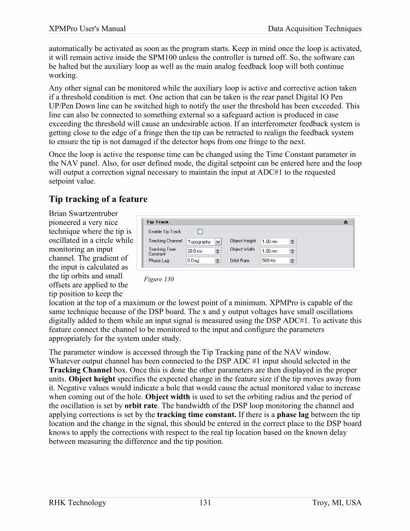
XPMPro User's Manual Data Acquisition Techniques
automatically be activated as soon as the program starts. Keep in mind once the loop is activated, it will remain active inside the SPM100 unless the controller is turned off. So, the software can be halted but the auxiliary loop as well as the main analog feedback loop will both continue working.Any other signal can be monitored while the auxiliary loop is active and corrective action taken if a threshold condition is met. One action that can be taken is the rear panel Digital IO Pen UP/Pen Down line can be switched high to notify the user the threshold has been exceeded. This line can also be connected to something external so a safeguard action is produced in case exceeding the threshold will cause an undesirable action. If an interferometer feedback system is getting close to the edge of a fringe then the tip can be retracted to realign the feedback system to ensure the tip is not damaged if the detector hops from one fringe to the next. Once the loop is active the response time can be changed using the Time Constant parameter in the NAV panel. Also, for user defined mode, the digital setpoint can be entered here and the loop will output a correction signal necessary to maintain the input at ADC#1 to the requested setpoint value.
Tip tracking of a featureBrian Swartzentruber pioneered a very nice technique where the tip is oscillated in a circle while monitoring an input channel. The gradient of the input is calculated as the tip orbits and small offsets are applied to the tip position to keep the location at the top of a maximum or the lowest point of a minimum. XPMPro is capable of the same technique because of the DSP board. The x and y output voltages have small oscillations digitally added to them while an input signal is measured using the DSP ADC#1. To activate this feature connect the channel to be monitored to the input and configure the parameters appropriately for the system under study.
The parameter window is accessed through the Tip Tracking pane of the NAV window. Whatever output channel has been connected to the DSP ADC #1 input should selected in the Tracking Channel box. Once this is done the other parameters are then displayed in the proper units. Object height specifies the expected change in the feature size if the tip moves away from it. Negative values would indicate a hole that would cause the actual monitored value to increase when coming out of the hole. Object width is used to set the orbiting radius and the period of the oscillation is set by orbit rate. The bandwidth of the DSP loop monitoring the channel and applying corrections is set by the tracking time constant. If there is a phase lag between the tip location and the change in the signal, this should be entered in the correct place to the DSP board knows to apply the corrections with respect to the real tip location based on the known delay between measuring the difference and the tip position.
RHK Technology 131 Troy, MI, USA
Figure 130
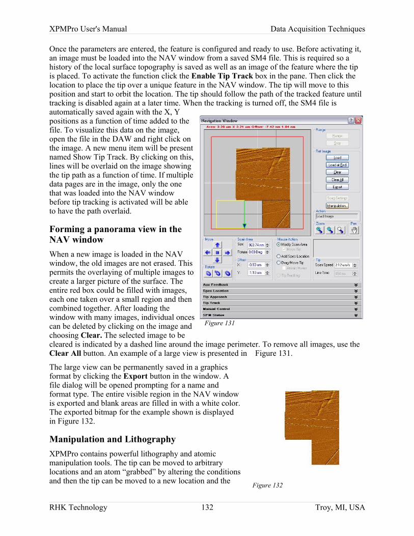
XPMPro User's Manual Data Acquisition Techniques
Once the parameters are entered, the feature is configured and ready to use. Before activating it, an image must be loaded into the NAV window from a saved SM4 file. This is required so a history of the local surface topography is saved as well as an image of the feature where the tip is placed. To activate the function click the Enable Tip Track box in the pane. Then click the location to place the tip over a unique feature in the NAV window. The tip will move to this position and start to orbit the location. The tip should follow the path of the tracked feature until tracking is disabled again at a later time. When the tracking is turned off, the SM4 file is automatically saved again with the X, Y positions as a function of time added to the file. To visualize this data on the image, open the file in the DAW and right click on the image. A new menu item will be present named Show Tip Track. By clicking on this, lines will be overlaid on the image showing the tip path as a function of time. If multiple data pages are in the image, only the one that was loaded into the NAV window before tip tracking is activated will be able to have the path overlaid.
Forming a panorama view in the NAV windowWhen a new image is loaded in the NAV window, the old images are not erased. This permits the overlaying of multiple images to create a larger picture of the surface. The entire red box could be filled with images, each one taken over a small region and then combined together. After loading the window with many images, individual onces can be deleted by clicking on the image and choosing Clear. The selected image to be cleared is indicated by a dashed line around the image perimeter. To remove all images, use the Clear All button. An example of a large view is presented in Figure 131.
The large view can be permanently saved in a graphics format by clicking the Export button in the window. A file dialog will be opened prompting for a name and format type. The entire visible region in the NAV window is exported and blank areas are filled in with a white color. The exported bitmap for the example shown is displayed in Figure 132.
Manipulation and LithographyXPMPro contains powerful lithography and atomic manipulation tools. The tip can be moved to arbitrary locations and an atom “grabbed” by altering the conditions and then the tip can be moved to a new location and the
RHK Technology 132 Troy, MI, USA
Figure 131
Figure 132
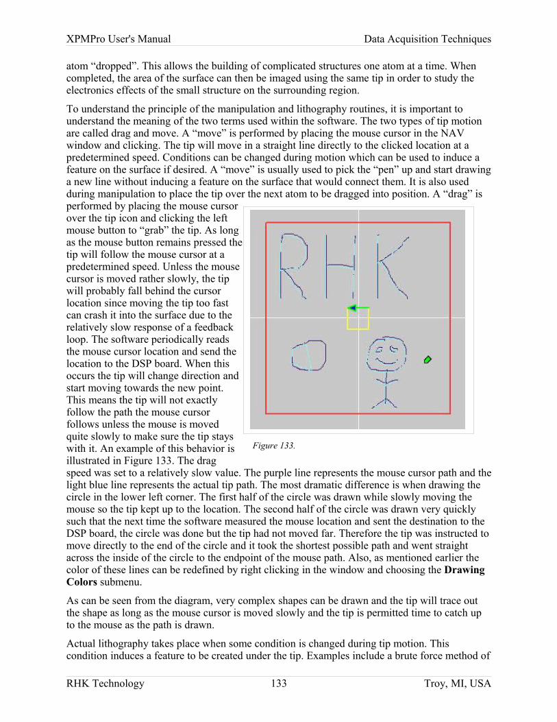
XPMPro User's Manual Data Acquisition Techniques
atom “dropped”. This allows the building of complicated structures one atom at a time. When completed, the area of the surface can then be imaged using the same tip in order to study the electronics effects of the small structure on the surrounding region.
To understand the principle of the manipulation and lithography routines, it is important to understand the meaning of the two terms used within the software. The two types of tip motion are called drag and move. A “move” is performed by placing the mouse cursor in the NAV window and clicking. The tip will move in a straight line directly to the clicked location at a predetermined speed. Conditions can be changed during motion which can be used to induce a feature on the surface if desired. A “move” is usually used to pick the “pen” up and start drawing a new line without inducing a feature on the surface that would connect them. It is also used during manipulation to place the tip over the next atom to be dragged into position. A “drag” is performed by placing the mouse cursor over the tip icon and clicking the left mouse button to “grab” the tip. As long as the mouse button remains pressed the tip will follow the mouse cursor at a predetermined speed. Unless the mouse cursor is moved rather slowly, the tip will probably fall behind the cursor location since moving the tip too fast can crash it into the surface due to the relatively slow response of a feedback loop. The software periodically reads the mouse cursor location and send the location to the DSP board. When this occurs the tip will change direction and start moving towards the new point. This means the tip will not exactly follow the path the mouse cursor follows unless the mouse is moved quite slowly to make sure the tip stays with it. An example of this behavior is illustrated in Figure 133. The drag speed was set to a relatively slow value. The purple line represents the mouse cursor path and the light blue line represents the actual tip path. The most dramatic difference is when drawing the circle in the lower left corner. The first half of the circle was drawn while slowly moving the mouse so the tip kept up to the location. The second half of the circle was drawn very quickly such that the next time the software measured the mouse location and sent the destination to the DSP board, the circle was done but the tip had not moved far. Therefore the tip was instructed to move directly to the end of the circle and it took the shortest possible path and went straight across the inside of the circle to the endpoint of the mouse path. Also, as mentioned earlier the color of these lines can be redefined by right clicking in the window and choosing the Drawing Colors submenu.
As can be seen from the diagram, very complex shapes can be drawn and the tip will trace out the shape as long as the mouse cursor is moved slowly and the tip is permitted time to catch up to the mouse as the path is drawn.
Actual lithography takes place when some condition is changed during tip motion. This condition induces a feature to be created under the tip. Examples include a brute force method of
RHK Technology 133 Troy, MI, USA
Figure 133.
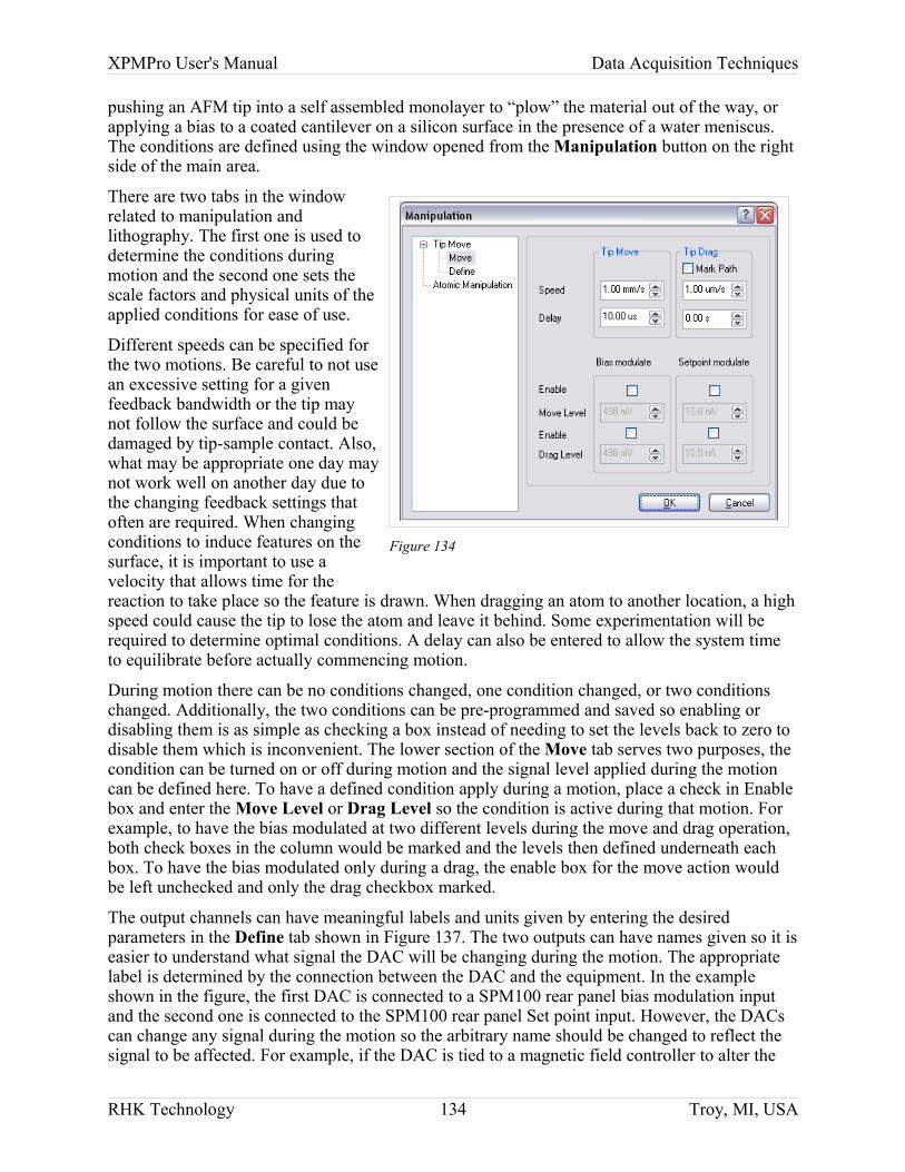
XPMPro User's Manual Data Acquisition Techniques
pushing an AFM tip into a self assembled monolayer to “plow” the material out of the way, or applying a bias to a coated cantilever on a silicon surface in the presence of a water meniscus. The conditions are defined using the window opened from the Manipulation button on the right side of the main area.
There are two tabs in the window related to manipulation and lithography. The first one is used to determine the conditions during motion and the second one sets the scale factors and physical units of the applied conditions for ease of use.
Different speeds can be specified for the two motions. Be careful to not use an excessive setting for a given feedback bandwidth or the tip may not follow the surface and could be damaged by tip-sample contact. Also, what may be appropriate one day may not work well on another day due to the changing feedback settings that often are required. When changing conditions to induce features on the surface, it is important to use a velocity that allows time for the reaction to take place so the feature is drawn. When dragging an atom to another location, a high speed could cause the tip to lose the atom and leave it behind. Some experimentation will be required to determine optimal conditions. A delay can also be entered to allow the system time to equilibrate before actually commencing motion.
During motion there can be no conditions changed, one condition changed, or two conditions changed. Additionally, the two conditions can be pre-programmed and saved so enabling or disabling them is as simple as checking a box instead of needing to set the levels back to zero to disable them which is inconvenient. The lower section of the Move tab serves two purposes, the condition can be turned on or off during motion and the signal level applied during the motion can be defined here. To have a defined condition apply during a motion, place a check in Enable box and enter the Move Level or Drag Level so the condition is active during that motion. For example, to have the bias modulated at two different levels during the move and drag operation, both check boxes in the column would be marked and the levels then defined underneath each box. To have the bias modulated only during a drag, the enable box for the move action would be left unchecked and only the drag checkbox marked.
The output channels can have meaningful labels and units given by entering the desired parameters in the Define tab shown in Figure 137. The two outputs can have names given so it is easier to understand what signal the DAC will be changing during the motion. The appropriate label is determined by the connection between the DAC and the equipment. In the example shown in the figure, the first DAC is connected to a SPM100 rear panel bias modulation input and the second one is connected to the SPM100 rear panel Set point input. However, the DACs can change any signal during the motion so the arbitrary name should be changed to reflect the signal to be affected. For example, if the DAC is tied to a magnetic field controller to alter the
RHK Technology 134 Troy, MI, USA
Figure 134
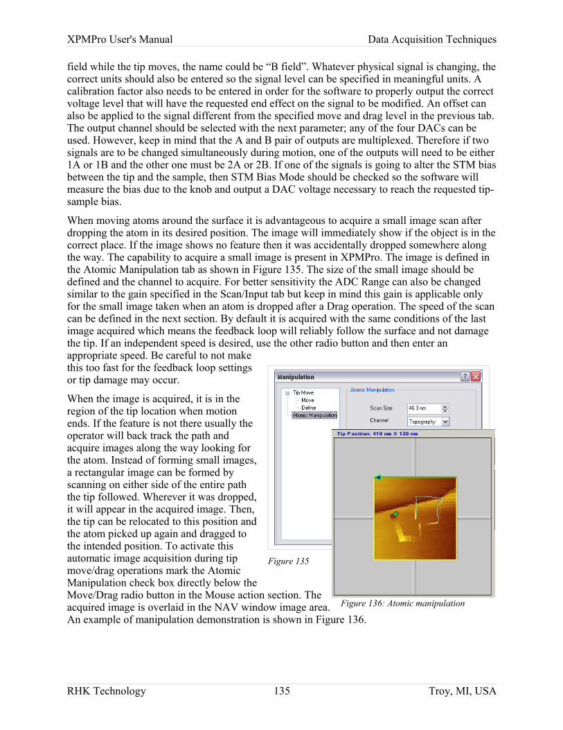
XPMPro User's Manual Data Acquisition Techniques
field while the tip moves, the name could be “B field”. Whatever physical signal is changing, the correct units should also be entered so the signal level can be specified in meaningful units. A calibration factor also needs to be entered in order for the software to properly output the correct voltage level that will have the requested end effect on the signal to be modified. An offset can also be applied to the signal different from the specified move and drag level in the previous tab. The output channel should be selected with the next parameter; any of the four DACs can be used. However, keep in mind that the A and B pair of outputs are multiplexed. Therefore if two signals are to be changed simultaneously during motion, one of the outputs will need to be either 1A or 1B and the other one must be 2A or 2B. If one of the signals is going to alter the STM bias between the tip and the sample, then STM Bias Mode should be checked so the software will measure the bias due to the knob and output a DAC voltage necessary to reach the requested tip-sample bias.
When moving atoms around the surface it is advantageous to acquire a small image scan after dropping the atom in its desired position. The image will immediately show if the object is in the correct place. If the image shows no feature then it was accidentally dropped somewhere along the way. The capability to acquire a small image is present in XPMPro. The image is defined in the Atomic Manipulation tab as shown in Figure 135. The size of the small image should be defined and the channel to acquire. For better sensitivity the ADC Range can also be changed similar to the gain specified in the Scan/Input tab but keep in mind this gain is applicable only for the small image taken when an atom is dropped after a Drag operation. The speed of the scan can be defined in the next section. By default it is acquired with the same conditions of the last image acquired which means the feedback loop will reliably follow the surface and not damage the tip. If an independent speed is desired, use the other radio button and then enter an appropriate speed. Be careful to not make this too fast for the feedback loop settings or tip damage may occur.
When the image is acquired, it is in the region of the tip location when motion ends. If the feature is not there usually the operator will back track the path and acquire images along the way looking for the atom. Instead of forming small images, a rectangular image can be formed by scanning on either side of the entire path the tip followed. Wherever it was dropped, it will appear in the acquired image. Then, the tip can be relocated to this position and the atom picked up again and dragged to the intended position. To activate this automatic image acquisition during tip move/drag operations mark the Atomic Manipulation check box directly below the Move/Drag radio button in the Mouse action section. The acquired image is overlaid in the NAV window image area. An example of manipulation demonstration is shown in Figure 136.
RHK Technology 135 Troy, MI, USA
Figure 135
Figure 136: Atomic manipulation
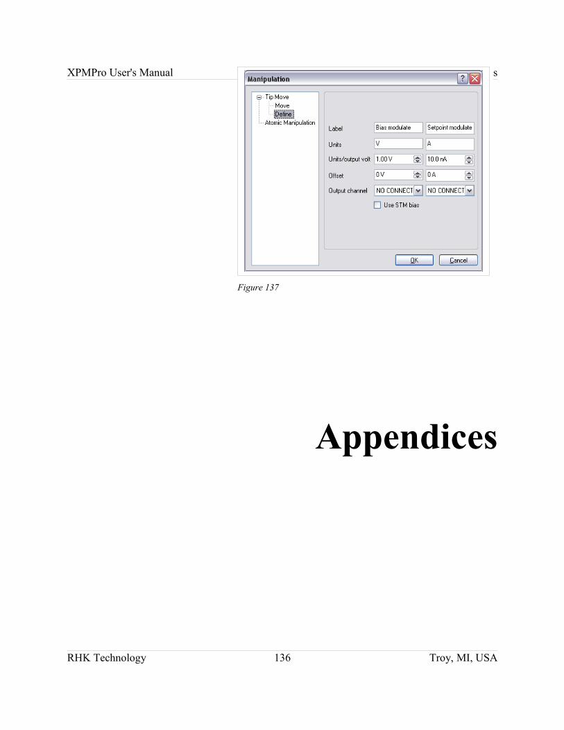
XPMPro User's Manual Appendices
Appendices
RHK Technology 136 Troy, MI, USA
Figure 137
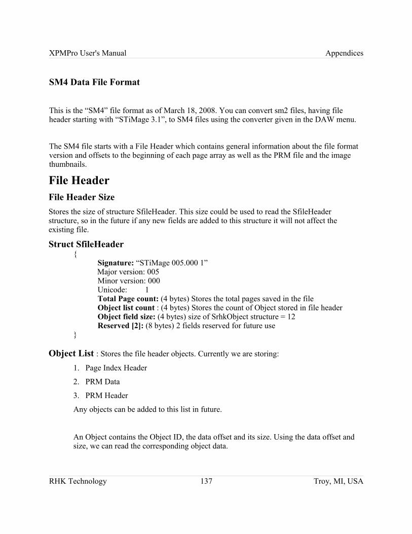
XPMPro User's Manual Appendices
SM4 Data File Format
This is the “SM4” file format as of March 18, 2008. You can convert sm2 files, having file header starting with “STiMage 3.1”, to SM4 files using the converter given in the DAW menu.
The SM4 file starts with a File Header which contains general information about the file format version and offsets to the beginning of each page array as well as the PRM file and the image thumbnails.
File HeaderFile Header Size
Stores the size of structure SfileHeader. This size could be used to read the SfileHeader structure, so in the future if any new fields are added to this structure it will not affect the existing file.
Struct SfileHeader{
Signature: “STiMage 005.000 1” Major version: 005Minor version: 000Unicode: 1Total Page count: (4 bytes) Stores the total pages saved in the fileObject list count : (4 bytes) Stores the count of Object stored in file headerObject field size: (4 bytes) size of SrhkObject structure = 12Reserved [2]: (8 bytes) 2 fields reserved for future use
}
Object List : Stores the file header objects. Currently we are storing:
1. Page Index Header
2. PRM Data
3. PRM Header
Any objects can be added to this list in future.
An Object contains the Object ID, the data offset and its size. Using the data offset and size, we can read the corresponding object data.
RHK Technology 137 Troy, MI, USA

XPMPro User's Manual Appendices
Struct SObject{
Object ID: (4 bytes) – Type of data storedOffset: (4 bytes) Data offsetSize: (4 bytes) size of the data
}
Defined Object Ids:Undefined - 0Page Index Header - 1Page Index Array - 2Page Header - 3Page Data - 4Image Drift Header - 5Image Drift - 6Spec Drift Header - 7Spec Drift Data (with X,Y coordinates) - 8Color Info - 9String data - 10Tip Track Header - 11Tip Track Data - 12PRM - 13Thumbnail - 14 //Not implementedPRM Header - 15Thumbnail Header - 16
The basic unit in a file is a “page”. A page can be a single image, a single spectrum, or a group of spectra. One file may have many pages, including combinations of image and spectral data. Each page starts with a header to provide the information about the page layout within the file as well as an array to point to each page.
Page Index HeaderThe page index header stores the details of page index array, which contains the array of page offsets and other info. Using the Index array we can locate the required page data, thumbnail data for the respective page, etc without reading the entire SM4 file.
Page count: (Data type long) Bytes used 8 bytesStores the number of pages in the page index array
Object List Count:
Stores the count of objects stored after page index header
RHK Technology 138 Troy, MI, USA

XPMPro User's Manual Appendices
Reserved [2] : (8 bytes)
Two fields reserved for future use
Object List:
Stores the Index header objects. Currently we are storing one object:
1. Page Index Array:
Page Index ArrayBased on the page count, an array of SPageIndex structure will be stored after the Page Index header.
Struct SPageIndex{Page ID: Unique ID for each PagePage Data Type: The type of data stored with the page. Defined types are.
0 = image data1 = line/spectral data2 = xy_data3 = annotated line/spectral data (see note below)4 = text_data5 = text_annotate6 = Sequential_data
Page Source Type: Identifies the page source type. The defined types are given below0 = raw page 1 = processed page 2 = calculated page3 = imported page
Object List Count: Stores the count of Objects stored after each the Page IndexMinor Version: (4 bytes) stores the minor version of the file (minor version = 0)}
Object List: Stores the Page Index objects. Currently we are storing:1. Page Header 2. Page Data3. Thumbnail4. Thumbnail header
After this begins a page of data. Here is a simple diagram that outlines the layout of each page of
RHK Technology 139 Troy, MI, USA
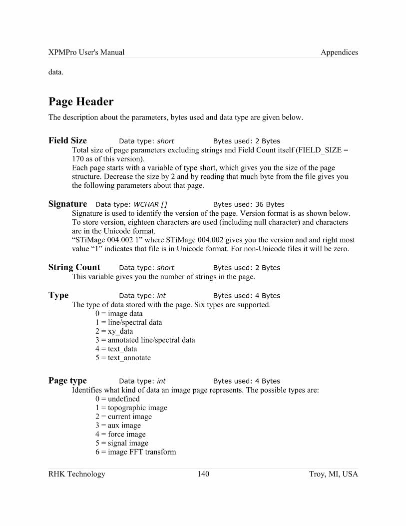
XPMPro User's Manual Appendices
data.
Page HeaderThe description about the parameters, bytes used and data type are given below.
Field Size Data type: short Bytes used: 2 BytesTotal size of page parameters excluding strings and Field Count itself (FIELD_SIZE = 170 as of this version).Each page starts with a variable of type short, which gives you the size of the page structure. Decrease the size by 2 and by reading that much byte from the file gives you the following parameters about that page.
Signature Data type: WCHAR [] Bytes used: 36 BytesSignature is used to identify the version of the page. Version format is as shown below. To store version, eighteen characters are used (including null character) and characters are in the Unicode format.“STiMage 004.002 1” where STiMage 004.002 gives you the version and and right most value “1” indicates that file is in Unicode format. For non-Unicode files it will be zero.
String Count Data type: short Bytes used: 2 BytesThis variable gives you the number of strings in the page.
Type Data type: int Bytes used: 4 BytesThe type of data stored with the page. Six types are supported.
0 = image data1 = line/spectral data2 = xy_data3 = annotated line/spectral data 4 = text_data5 = text_annotate
Page type Data type: int Bytes used: 4 BytesIdentifies what kind of data an image page represents. The possible types are:
0 = undefined1 = topographic image2 = current image3 = aux image4 = force image5 = signal image6 = image FFT transform
RHK Technology 140 Troy, MI, USA
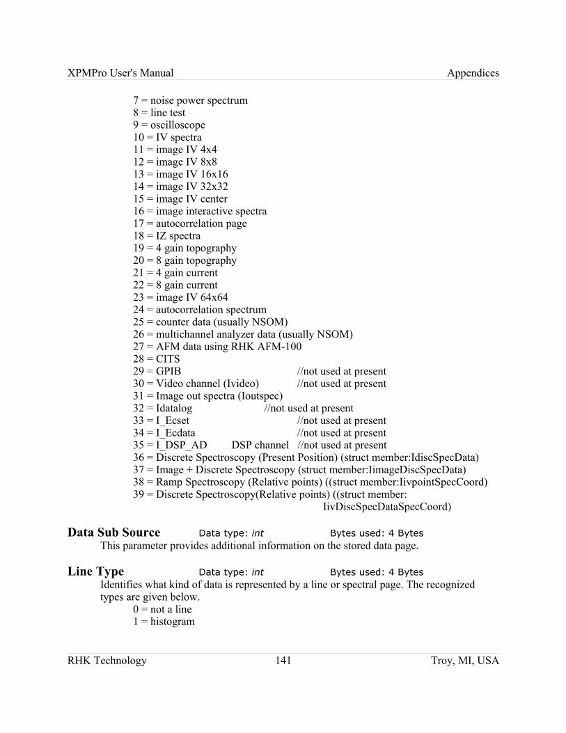
XPMPro User's Manual Appendices
7 = noise power spectrum8 = line test9 = oscilloscope10 = IV spectra11 = image IV 4x412 = image IV 8x813 = image IV 16x1614 = image IV 32x3215 = image IV center16 = image interactive spectra17 = autocorrelation page18 = IZ spectra19 = 4 gain topography20 = 8 gain topography21 = 4 gain current22 = 8 gain current23 = image IV 64x6424 = autocorrelation spectrum25 = counter data (usually NSOM)26 = multichannel analyzer data (usually NSOM)27 = AFM data using RHK AFM-10028 = CITS 29 = GPIB //not used at present30 = Video channel (Ivideo) //not used at present31 = Image out spectra (Ioutspec)32 = Idatalog //not used at present33 = I_Ecset //not used at present34 = I_Ecdata //not used at present35 = I_DSP_AD DSP channel //not used at present36 = Discrete Spectroscopy (Present Position) (struct member:IdiscSpecData)37 = Image + Discrete Spectroscopy (struct member:IimageDiscSpecData)38 = Ramp Spectroscopy (Relative points) ((struct member:IivpointSpecCoord)39 = Discrete Spectroscopy(Relative points) ((struct member:
IivDiscSpecDataSpecCoord)
Data Sub Source Data type: int Bytes used: 4 BytesThis parameter provides additional information on the stored data page.
Line Type Data type: int Bytes used: 4 BytesIdentifies what kind of data is represented by a line or spectral page. The recognized types are given below.
0 = not a line1 = histogram
RHK Technology 141 Troy, MI, USA

XPMPro User's Manual Appendices
2 = cross section3 = line test4 = oscilloscope5 = reserved6 = noise power spectrum7 = I-V spectrum8 = I-Z spectrum9 = image X average10 = image Y average11 = noise autocorrelation spectrum12 = multichannel analyzer data13 = renormalized IV data from variable gap IV14 = image histogram spectra15 = image cross section16 = image average17 = Image Cross Section (Gsection_fdata)18 = Image Out Spectra (Goutspec)19 = Datalog Spectrum (Gdatalog) //Not used at present20 = Gxy //Not used at present21 = Electro chemistry (Gechem) //Not used at present22 = Discrete Spectroscopy. (Gdiscspec_data)
X,Y Coordinates Width and Height Data type: structure RECT_SIZE Bytes used: 16 Bytes
typedef struct tagRECT_SIZE{ int m_nX; // X corner int m_nY; // Y corner int m_nWidth; // Width int m_nHeight; // Height} RECT_SIZE;
m_nWidth: The number of pixels or points in the X direction for an image page, or the number of points per spectra/line for line pages.
m_nHeight: The number of pixels or points in the Y direction for an image page, or the number of spectra stored in the page
Source Type Data type: int Bytes used: 4 BytesIdentifies the page source type. The recognized types are given below
0 = raw page 1 = processed page
RHK Technology 142 Troy, MI, USA

XPMPro User's Manual Appendices
2 = calculated page3 = imported page
Image Type Data type: int Bytes used: 4 BytesIdentifies what kind of data is represented by an image
0 = normal image1 = autocorrelation image
Scan Data type: int Bytes used: 4 BytesThe scan direction (direction of data acquisition) in an image. It is not meaningful for an I-V curve, for example. On the computer screen X is horizontal and Y is vertical.
0 = right1 = left2 = up3 = down
Group ID Data type: int Bytes used: 4 BytesAn Integer value to identify the pages acquired during an acquisition. All the pages acquired during an acquisition will get the same group id.
Page Data Size Data type: unsigned long Bytes used: 4 BytesThe total number of data bytes in the data section. It is equal to m_nWidth * m_nHeight* sizeof (long int). For Float data it should be m_nWidth * m_nHeight* sizeof (float). In case of Disc. Spectroscopy, the datasize = ((m_nWidth * m_nHeight ) + m_nWidth) * size of (float). Additional size of width is to store the user enterd voltage values for a page.
Page will have float data if the Line Type is any one of the following:
Gdatalog, Gechem, Givnorm, Gfft_power, Gautocorr, Goutspec
Gdiscspec_data, Ghistogram, Gx_ave,Gy_ave
All image data is stored as 32 bit signed integers. Most spectral data is either 32 bit signed integers or floating point such as power spectra and autocorrelation spectra point.
Minimum Z Value Data type: Unsigned long Bytes used: 4 BytesStores the minimum Z Value.
Maximum Z Value Data type: Unsigned long Bytes used: 4 BytesStores the Maximum Z Value.
X Scale, Y Scale, Z Scale Data type: float Bytes used: 4 Bytes each.
RHK Technology 143 Troy, MI, USA

XPMPro User's Manual Appendices
The X, Y, Z physical units per pixel or bit.
X Y Scale Data type: float Bytes used: 4 Bytes This is the change in X in physical units per Y line. This is used for drift Correction and is 0 for newly acquired images.
X OffsetY OffsetZ Offset Data type: float Bytes used: 4 Bytes each
The origin of the X value, or the X coord of the image center. The physical unit is ' XOffset ' + 'XScale ' * (x number) The Y and Z offset are similar.Z is the acquired data. X and Y are the image coordinates for 3D data. 2D data is plotted as X-Z. The Y coordinate is just an index. For an I-V curve, for example, if 4 curves are acquired, X is in Volts, Z in Amps and Y is 0, 1, 2 or 3. In a force image X and Y are meters and Z is Newton.
Period Data type: float Bytes used: 4 BytesThe time to acquire each data point.
Bias Data type: float Bytes used: 4 BytesThe sample bias in volts (not relevant for most AFM data)
Current Data type: float Bytes used: 4 BytesThe absolute value of the sample current in amps (not relevant for most AFM data)
Angle Data type: float Bytes used: 4 BytesThe angle by which the image is rotated. (Normally 0)
ColorInfoList Count Data type: int Bytes used: 4 Bytes
Stores the number of color info.
Grid X Size Data type: int Bytes used: 4 Bytes
Spectral grid X size
Grid Y Size Data type: int Bytes used: 4 Bytes
Spectral grid Y size
RHK Technology 144 Troy, MI, USA

XPMPro User's Manual Appendices
Object list count Stores the count of Objects stored after the Page Header
Reserved [16]: (16 * 4 bytes = 64) Reserved for future use
Object list: Stores the Page header objects, Currently we are storing 1. String Data2. Image Drift header3. Image Drift Data4. Spec Drift Header5. Spectral Data6. Color Info7. Tip-track Info Header8. Tip-track Data
TEXT STRINGSStringCnt gives you the number of strings in the current page. Each string is written to file by first writing the string length, then the string. So when you read, first read a short value, which gives you the string length, then read that much bytes which represents the string.
strLabel: String that goes on the top of the plot window, like “Current Image”.strSystemText: A comment describing the data. strSessionText: General session comments.strUserText: User comments.strPath: Path and name of the SM4 file, which holds the page.strDate: Stores the date at which data is acquired.strTime: Stores the time at which data is acquired.strXUnits: Physical units of that axis, like “m” or “A”.strYUnits: Physical units of that axis.strZUnits: Physical units of that axis.strXLabel.strYLabel.strStatusChannelText: Status channel text
strCompletedLineCount: Completed line count info. This string contains the last saved line count for an image data page. For all other pages, this value will be zero.
StrOverSamplingCount: This string contains the Oversampling count for image data pages. For all other pages this value will be zero.
StrSlicedVoltage : The voltage at which the sliced image is created from the spectra
RHK Technology 145 Troy, MI, USA

XPMPro User's Manual Appendices
page. This string will be empty for pages other than sliced image pages.
StrPLLProStatus : This string contains the PLLPro status text, if the operating mode is selected as PLLPro master or PLLPro user.
Page Header – Sequential Data PageThe sequential data page is generic page in which the page data is a (m,n) array. Where ‘m’ is the number of parameters in the array and ‘n’ is the array count. The array elements will be all float type. The parameter info is stored in the page header. (Sequential Data Header).
If the PageDataType is Sequential_data, then Page header contains the following parameters.
Data Type Data Type: int Bytes used:(4 Bytes)
Type of the Data stored in the page. The defined types are
1 = Spec Drift (Stores the SSpecInfo structure as the Data, Param Count gives the number of float data in this structure.)
2 = Image Drift (Stores the SImageDrift structure as the Data, Param Count gives the number of float data in this structure.)
3 = Tip Track (Stores the StipTrackInfo structure as the Data, Param Count gives the number of float data in this structure.)
Data Length Data Type: int Bytes used: (4 Bytes)
Stores the Array Size
Param Count Data Type: int Bytes used: (4 Bytes)
Number of parameters (float data ) in an array element
Object List Count Data Type : unsigned int Bytes used: (4 Bytes)
Count of objects stored after the header
Data Info Size Data Type : unsigned int Bytes used: (4 Bytes)
Size of the SXdataInfo structure – excluding the string
Data Info String Count Data Type : unsigned int Bytes used: (4 Bytes)
Number of strings in the SXdataInfo structure
Object ListList of object stored after the sequential data header. Currently we are storing
RHK Technology 146 Troy, MI, USA

XPMPro User's Manual Appendices
1. Image Drift Header2. Spec Drift Header 3. Tip Track header
struct StipTrackInfoHeader{
FILETIME m_ftStartTime;float m_fFeatureHeight;float m_fFeatureWidth;float m_fTimeConstant;float m_fCycleRate;float m_fPhaseLag;unsigned int m_unStringCount;unsigned int m_unTipTrackInfoCount; //Stores the array size of the StipTrackInforhk_string m_szChannel;
} STipTrackInfoHeader;
struct StipTrackInfo //Array of this structure will be stored in the tip-track data{
float m_fCumulativeTime;float m_fTime; float m_fdX;float m_fdY;
}STipTrackInfo;
Data InfoAn array of Data Info is stored after the page header object list. It contains the information about each parameter stored in the page data. The following are the parameters in this structure
1. Param gain : Data Type float Bytes used: (4 bytes)2. StrLabel: (Data Type : string, the string size will be written before the string (2
bytes))Name of the parameter
3. strUnit: ( Data Type : string) Unit of the Parameter
The above details will be repeated for ‘n’ time where n is the ‘Param Count’
PAGE DATA Page Data size and file Offset can be obtained from the Page data Object Stored in the
RHK Technology 147 Troy, MI, USA
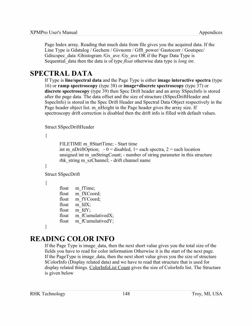
XPMPro User's Manual Appendices
Page Index array. Reading that much data from file gives you the acquired data. If the Line Type is Gdatalog / Gechem / Givnorm / Gfft_power/ Gautocorr / Goutspec/ Gdiscspec_data /Ghistogram /Gx_ave /Gy_ave OR if the Page Data Type is Sequential_data then the data is of type float otherwise data type is long int.
SPECTRAL DATAIf Type is line/spectral data and the Page Type is either image interactive spectra (type 16) or ramp spectroscopy (type 38) or image+discrete spectroscopy (type 37) or discrete spectroscopy (type 39) then Spec Drift header and an array SSpecInfo is stored after the page data. The data offset and the size of structure (SSpecDriftHeader and SspecInfo) is stored in the Spec Drift Header and Spectral Data Object respectively in the Page header object list. m_nHeight in the Page header gives the array size. If spectroscopy drift correction is disabled then the drift info is filled with default values.
Struct SSpecDriftHeader
{
FILETIME m_ftStartTime; - Start time int m_nDriftOption; - 0 = disabled, 1= each spectra, 2 = each locationunsigned int m_unStringCount; - number of string parameter in this structurerhk_string m_szChannel; - drift channel name
}
Struct SSpecDrift
{float m_fTime;float m_fXCoord;float m_fYCoord;float m_fdX;float m_fdY;float m_fCumulativedX;float m_fCumulativedY;
}
READING COLOR INFOIf the Page Type is image_data, then the next short value gives you the total size of the fields you have to read for color information Otherwise it is the start of the next page.If the PageType is image_data, then the next short value gives you the size of structure SColorInfo (Display related data) and we have to read that structure that is used for display related things. ColorInfoList Count gives the size of ColorInfo list. The Structure is given below
RHK Technology 148 Troy, MI, USA
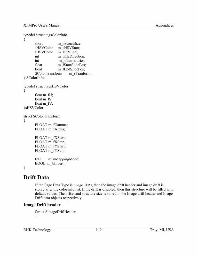
XPMPro User's Manual Appendices
typedef struct tagsColorInfo{
short m_nStructSize;sHSVColor m_sHSVStart;sHSVColor m_HSVEnd;int m_nClrDirection;int m_nNumEntries;float m_fStartSlidePos;float m_fEndSlidePos;SColorTransform m_sTranform;
} SColorInfo;
typedef struct tagsHSVColor{
float m_fH;float m_fS;float m_fV;
}sHSVColor;
struct SColorTransform{
FLOAT m_fGamma;FLOAT m_fAlpha;
FLOAT m_fXStart;FLOAT m_fXStop;FLOAT m_fYStart;FLOAT m_fYStop;
INT m_nMappingMode;BOOL m_bInvert;
}
Drift DataIf the Page Data Type is image_data, then the image drift header and image drift is stored after the color info list. If the drift is disabled, then this structure will be filled with default values. The offset and structure size is stored in the Image drift header and Image Drift data objects respectively.
Image Drift headerStruct SimageDriftHeader{
RHK Technology 149 Troy, MI, USA
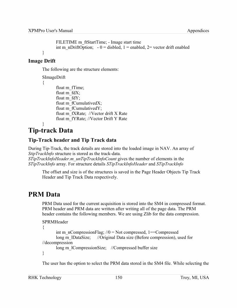
XPMPro User's Manual Appendices
FILETIME m_ftStartTime; - Image start timeint m_nDriftOption; - 0 = disbled, 1 = enabled, 2= vector drift enabled
}
Image Drift The following are the structure elements:
SImageDrift{
float m_fTime;float m_fdX;float m_fdY;float m_fCumulativedX;float m_fCumulativedY; float m_fXRate; //Vector drift X Ratefloat m_fYRate; //Vector Drift Y Rate
}Tip-track DataTip-Track header and Tip Track dataDuring Tip-Track, the track details are stored into the loaded image in NAV. An array of StipTrackInfo structure is stored as the track-data. STipTrackInfoHeader.m_unTipTrackInfoCount gives the number of elements in the STipTrackInfo array. For structure details STipTrackInfoHeader and STipTrackInfo
The offset and size is of the structures is saved in the Page Header Objects Tip Track Header and Tip Track Data respectively.
PRM DataPRM Data used for the current acquisition is stored into the SM4 in compressed format. PRM header and PRM data are written after writing all of the page data. The PRM header contains the following members. We are using Zlib for the data compression.
SPRMHeader{
int m_nCompressionFlag; //0 = Not compressed, 1==Compressedlong m_lDataSize; //Original Data size (Before compression), used for
//decompressionlong m_lCompressionSize; //Compressed buffer size
}
The user has the option to select the PRM data stored in the SM4 file. While selecting the
RHK Technology 150 Troy, MI, USA

XPMPro User's Manual Appendices
PRM data from SM4, it will be saved into the application path with the SM4 filename.
Thumbnail Header and Thumbnail DataIn a DAW, instead of reading the entire page data to display the thumbnail, we are storing the reduced page data as thumbnail data for each page in SM4 file. The thumbnail data size is stored in the thumbnail header. The offset and size of the thumbnail header and data is stored in the Page index objects Thumbnail header (page type= 17) and Thumbnail (page type= 15) respectively. Using this offset we can locate the thumbnail data in Sm4.
For an image page, if the scan resolution (X or Y) is more than 128 then the page data is averaged and reduced to Min (128, X Size) and Min (128, Y Size) pixels and is stored as thumbnail data.
For a graph page, the curve average is stored as the thumbnail data.
The Width (X Size) and Height (Y Size) is stored inside the thumbnail header.
SThumbnailHeader{
int m_nWidth; //Points per lineint m_nHeight; //Lines per frameint m_nFormat; //=0 Raw data
}
The format represents the thumbnail data format. Currently, we are supporting only raw data. In DAW, if the thumbnail data is present, then it reads the thumbnail data and display (Page data will not be read in this case). If thumbnail data is not present, then it reads page data and display.
RHK Technology 151 Troy, MI, USA
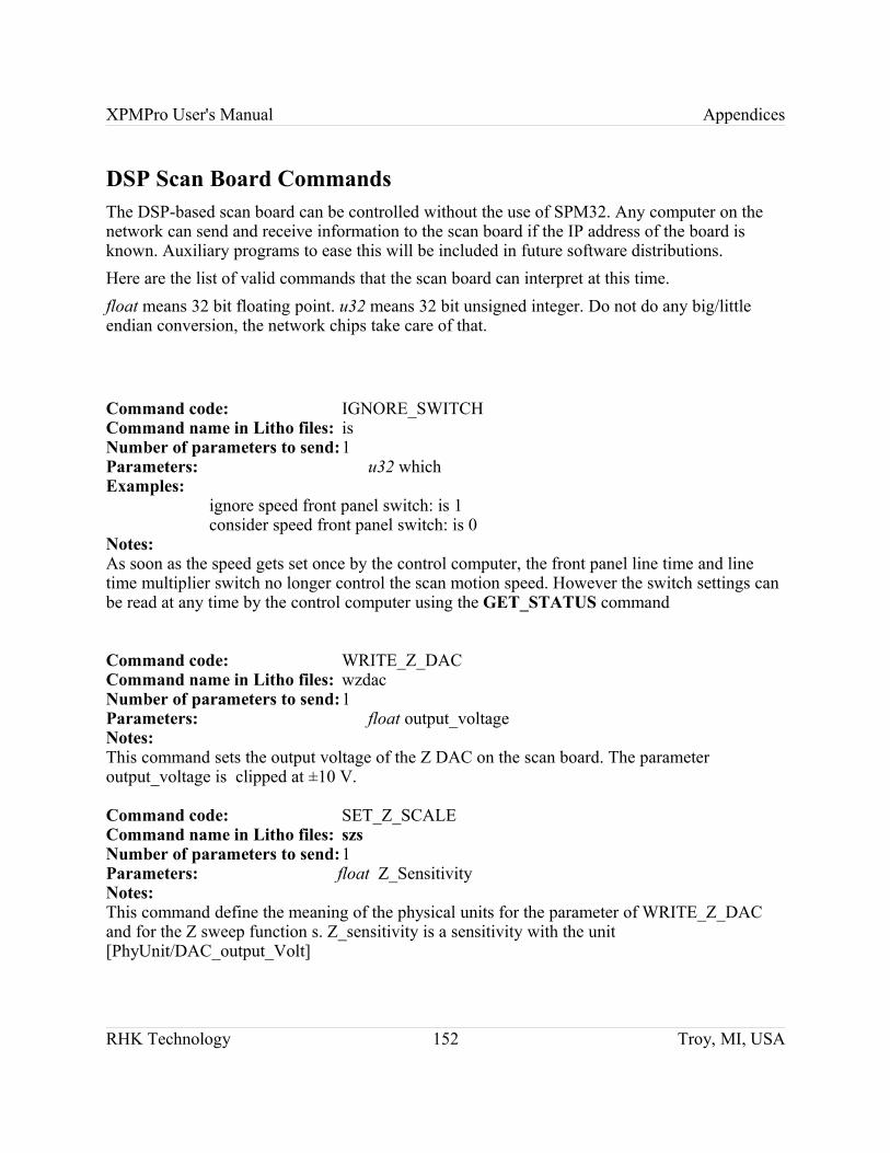
XPMPro User's Manual Appendices
DSP Scan Board CommandsThe DSP-based scan board can be controlled without the use of SPM32. Any computer on the network can send and receive information to the scan board if the IP address of the board is known. Auxiliary programs to ease this will be included in future software distributions. Here are the list of valid commands that the scan board can interpret at this time.float means 32 bit floating point. u32 means 32 bit unsigned integer. Do not do any big/little endian conversion, the network chips take care of that.
Command code: IGNORE_SWITCHCommand name in Litho files: isNumber of parameters to send:1Parameters: u32 which Examples:
ignore speed front panel switch: is 1consider speed front panel switch: is 0
Notes:As soon as the speed gets set once by the control computer, the front panel line time and line time multiplier switch no longer control the scan motion speed. However the switch settings can be read at any time by the control computer using the GET_STATUS command
Command code: WRITE_Z_DACCommand name in Litho files: wzdacNumber of parameters to send:1Parameters: float output_voltage Notes:This command sets the output voltage of the Z DAC on the scan board. The parameter output_voltage is clipped at ±10 V.
Command code: SET_Z_SCALECommand name in Litho files: szsNumber of parameters to send:1Parameters: float Z_SensitivityNotes:This command define the meaning of the physical units for the parameter of WRITE_Z_DAC and for the Z sweep function s. Z_sensitivity is a sensitivity with the unit [PhyUnit/DAC_output_Volt]
RHK Technology 152 Troy, MI, USA
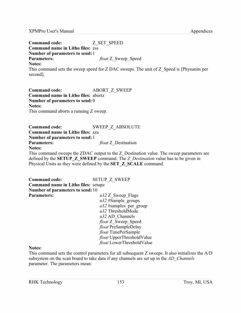
XPMPro User's Manual Appendices
Command code: Z_SET_SPEEDCommand name in Litho files: zssNumber of parameters to send:1Parameters: float Z_Sweep_Speed Notes:This command sets the sweep speed for Z DAC sweeps. The unit of Z_Speed is [Physunits per second].
Command code: ABORT_Z_SWEEPCommand name in Litho files: abortzNumber of parameters to send:0Notes:This command aborts a running Z sweep.
Command code: SWEEP_Z_ABSOLUTECommand name in Litho files: szaNumber of parameters to send:1Parameters: float Z_DestinationNotes:This command sweeps the ZDAC output to the Z_Destination value. The sweep parameters are defined by the SETUP_Z_SWEEP command. The Z_Destination value has to be given in Physical Units as they were defined by the SET_Z_SCALE command.
Command code: SETUP_Z_SWEEPCommand name in Litho files: setupzNumber of parameters to send:10Parameters: u32 Z_Sweep_Flags
u32 #Sample_groups u32 #samples_per_group u32 ThresholdMode u32 AD_Channels float Z_Sweep_Speed float PreSampleDelay float TimePerSample float UpperThresholdValue float LowerThresholdValue
Notes:This command sets the control parameters for all subsequent Z sweeps. It also initializes the A/D subsystem on the scan board to take data if any channels are set up in the AD_Channels parameter. The parameters mean:
RHK Technology 153 Troy, MI, USA
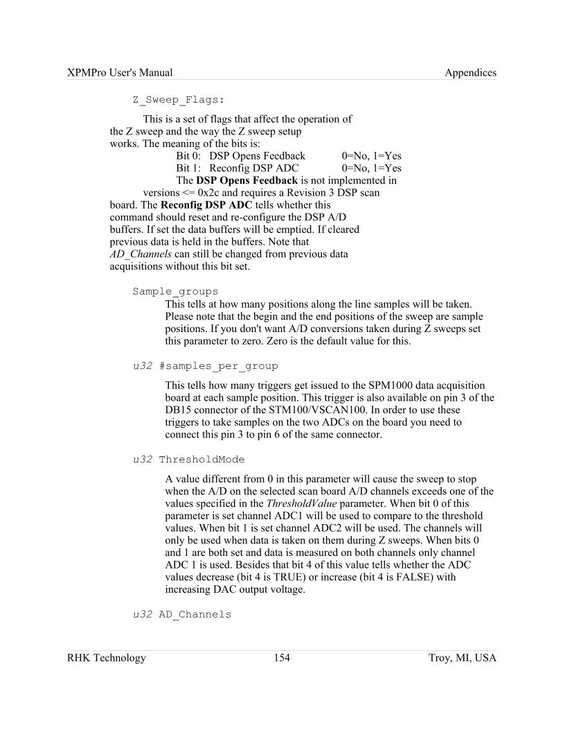
XPMPro User's Manual Appendices
Z_Sweep_Flags:
This is a set of flags that affect the operation of the Z sweep and the way the Z sweep setup works. The meaning of the bits is:
Bit 0: DSP Opens Feedback 0=No, 1=YesBit 1: Reconfig DSP ADC 0=No, 1=YesThe DSP Opens Feedback is not implemented in
versions <= 0x2c and requires a Revision 3 DSP scan board. The Reconfig DSP ADC tells whether this command should reset and re-configure the DSP A/D buffers. If set the data buffers will be emptied. If cleared previous data is held in the buffers. Note that AD_Channels can still be changed from previous data acquisitions without this bit set.
Sample_groupsThis tells at how many positions along the line samples will be taken. Please note that the begin and the end positions of the sweep are sample positions. If you don't want A/D conversions taken during Z sweeps set this parameter to zero. Zero is the default value for this.
u32 #samples_per_group
This tells how many triggers get issued to the SPM1000 data acquisition board at each sample position. This trigger is also available on pin 3 of the DB15 connector of the STM100/VSCAN100. In order to use these triggers to take samples on the two ADCs on the board you need to connect this pin 3 to pin 6 of the same connector.
u32 ThresholdMode
A value different from 0 in this parameter will cause the sweep to stop when the A/D on the selected scan board A/D channels exceeds one of the values specified in the ThresholdValue parameter. When bit 0 of this parameter is set channel ADC1 will be used to compare to the threshold values. When bit 1 is set channel ADC2 will be used. The channels will only be used when data is taken on them during Z sweeps. When bits 0 and 1 are both set and data is measured on both channels only channel ADC 1 is used. Besides that bit 4 of this value tells whether the ADC values decrease (bit 4 is TRUE) or increase (bit 4 is FALSE) with increasing DAC output voltage.
u32 AD_Channels
RHK Technology 154 Troy, MI, USA
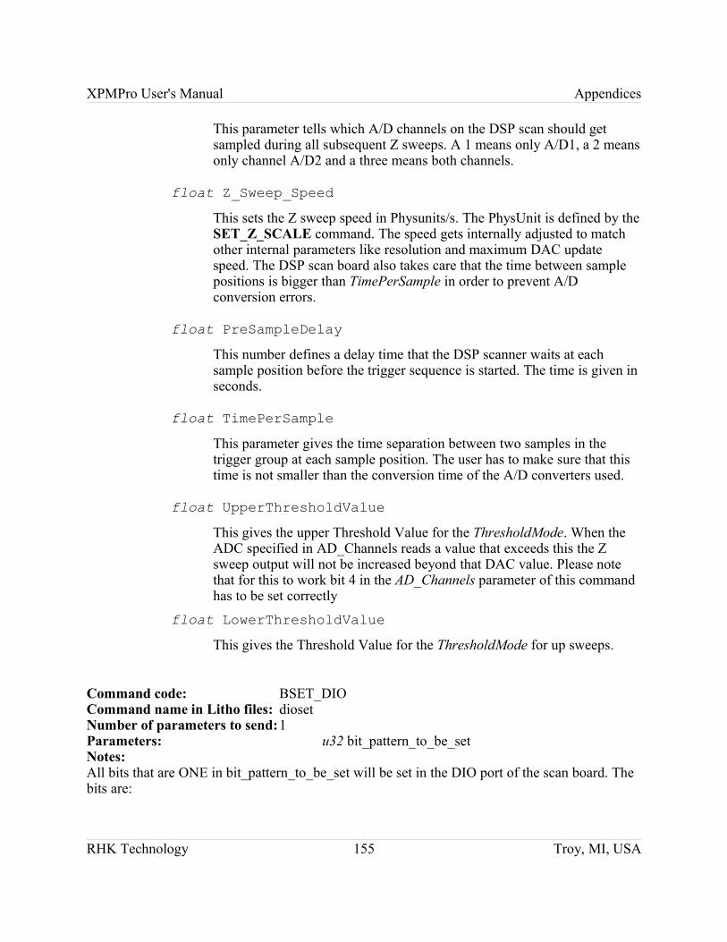
XPMPro User's Manual Appendices
This parameter tells which A/D channels on the DSP scan should get sampled during all subsequent Z sweeps. A 1 means only A/D1, a 2 means only channel A/D2 and a three means both channels.
float Z_Sweep_Speed
This sets the Z sweep speed in Physunits/s. The PhysUnit is defined by the SET_Z_SCALE command. The speed gets internally adjusted to match other internal parameters like resolution and maximum DAC update speed. The DSP scan board also takes care that the time between sample positions is bigger than TimePerSample in order to prevent A/D conversion errors.
float PreSampleDelay
This number defines a delay time that the DSP scanner waits at each sample position before the trigger sequence is started. The time is given in seconds.
float TimePerSample
This parameter gives the time separation between two samples in the trigger group at each sample position. The user has to make sure that this time is not smaller than the conversion time of the A/D converters used.
float UpperThresholdValue
This gives the upper Threshold Value for the ThresholdMode. When the ADC specified in AD_Channels reads a value that exceeds this the Z sweep output will not be increased beyond that DAC value. Please note that for this to work bit 4 in the AD_Channels parameter of this command has to be set correctly
float LowerThresholdValue
This gives the Threshold Value for the ThresholdMode for up sweeps.
Command code: BSET_DIOCommand name in Litho files: diosetNumber of parameters to send:1Parameters: u32 bit_pattern_to_be_setNotes:All bits that are ONE in bit_pattern_to_be_set will be set in the DIO port of the scan board. The bits are:
RHK Technology 155 Troy, MI, USA
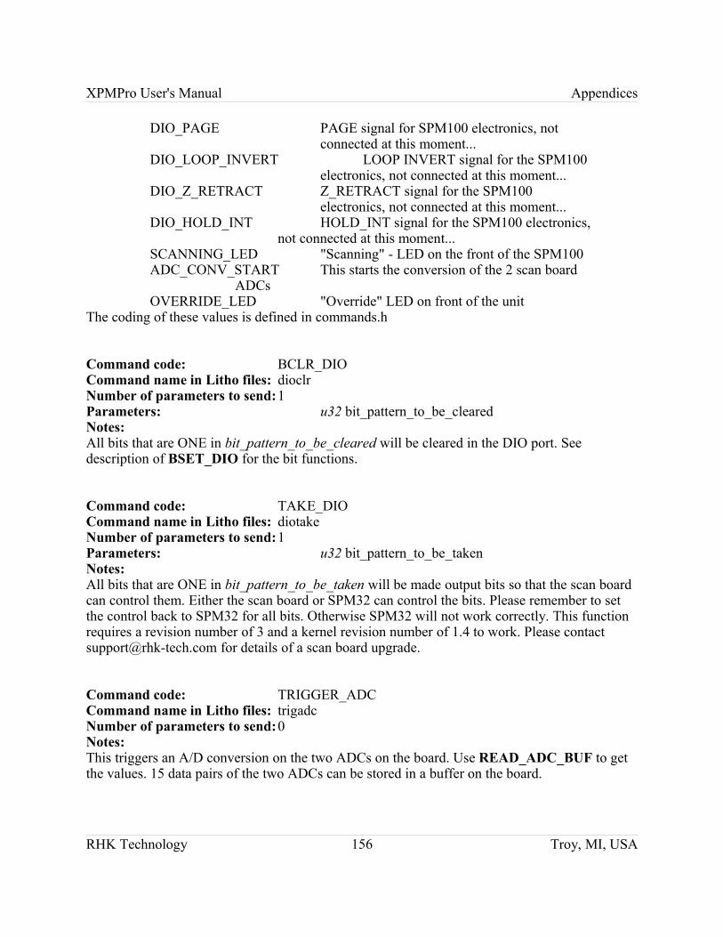
XPMPro User's Manual Appendices
DIO_PAGE PAGE signal for SPM100 electronics, not connected at this moment...
DIO_LOOP_INVERT LOOP INVERT signal for the SPM100 electronics, not connected at this moment...
DIO_Z_RETRACT Z_RETRACT signal for the SPM100 electronics, not connected at this moment...
DIO_HOLD_INT HOLD_INT signal for the SPM100 electronics, not connected at this moment...
SCANNING_LED "Scanning" - LED on the front of the SPM100ADC_CONV_START This starts the conversion of the 2 scan board
ADCs OVERRIDE_LED "Override" LED on front of the unit
The coding of these values is defined in commands.h
Command code: BCLR_DIOCommand name in Litho files: dioclrNumber of parameters to send:1Parameters: u32 bit_pattern_to_be_clearedNotes:All bits that are ONE in bit_pattern_to_be_cleared will be cleared in the DIO port. See description of BSET_DIO for the bit functions.
Command code: TAKE_DIOCommand name in Litho files: diotakeNumber of parameters to send:1Parameters: u32 bit_pattern_to_be_takenNotes:All bits that are ONE in bit_pattern_to_be_taken will be made output bits so that the scan board can control them. Either the scan board or SPM32 can control the bits. Please remember to set the control back to SPM32 for all bits. Otherwise SPM32 will not work correctly. This function requires a revision number of 3 and a kernel revision number of 1.4 to work. Please contact [email protected] for details of a scan board upgrade.
Command code: TRIGGER_ADC Command name in Litho files: trigadcNumber of parameters to send:0Notes:This triggers an A/D conversion on the two ADCs on the board. Use READ_ADC_BUF to get the values. 15 data pairs of the two ADCs can be stored in a buffer on the board.
RHK Technology 156 Troy, MI, USA

XPMPro User's Manual Appendices
Command code: READ_ADC_BUFCommand name in Litho files: gadcNumber of parameters to send:0Notes:This command reads the on-board A/D conversion buffers. The A/D conversions can be triggered via the external trigger input as well as via TRIGGER_ADC command. The data for the first 15 trigger events after a READ_ADC_BUF are stored in the buffer. This command uploads the data in the buffer and then empties it.
Command code: WRITE_ADC_BUFCommand name in Litho files: wadcNumber of parameters to send:variableNotes:This command writes "how_many" data points into the on-board A/D conversion buffers as if they were written by the Data Acquisition. The first u32 word in the reply is the number of A/D samples that get sent down to the board. This command is intended for testing and for writing the output data for the replay mode
Command code: GET GAINS
Command name in Litho files: gg
Number of parameters to send: 0
Note:
This command returns a table that contains the high voltage gain parameters that are burned into the chassis EEPROM of the SPM100 units. Please note that a reading of 6553.5 indicates that the EEPROM does not contain the correct header revision. In this case the information might be in the modifications field of the EEPROM header. The data structure returned by the GET GAINS command looks like this:
[0] u32 the GET_GAINS command code
[1] float X Offset Gain
[2] float X Scan Gain
[3] float Y Offset Gain
[4] float Y Scan Gain
[5] float Z Offset Gain
[6] float Z Scan Gain
Command code: GET_STATUSCommand name in Litho files: gsNumber of parameters to send:0Parameters: noneNotes:
RHK Technology 157 Troy, MI, USA
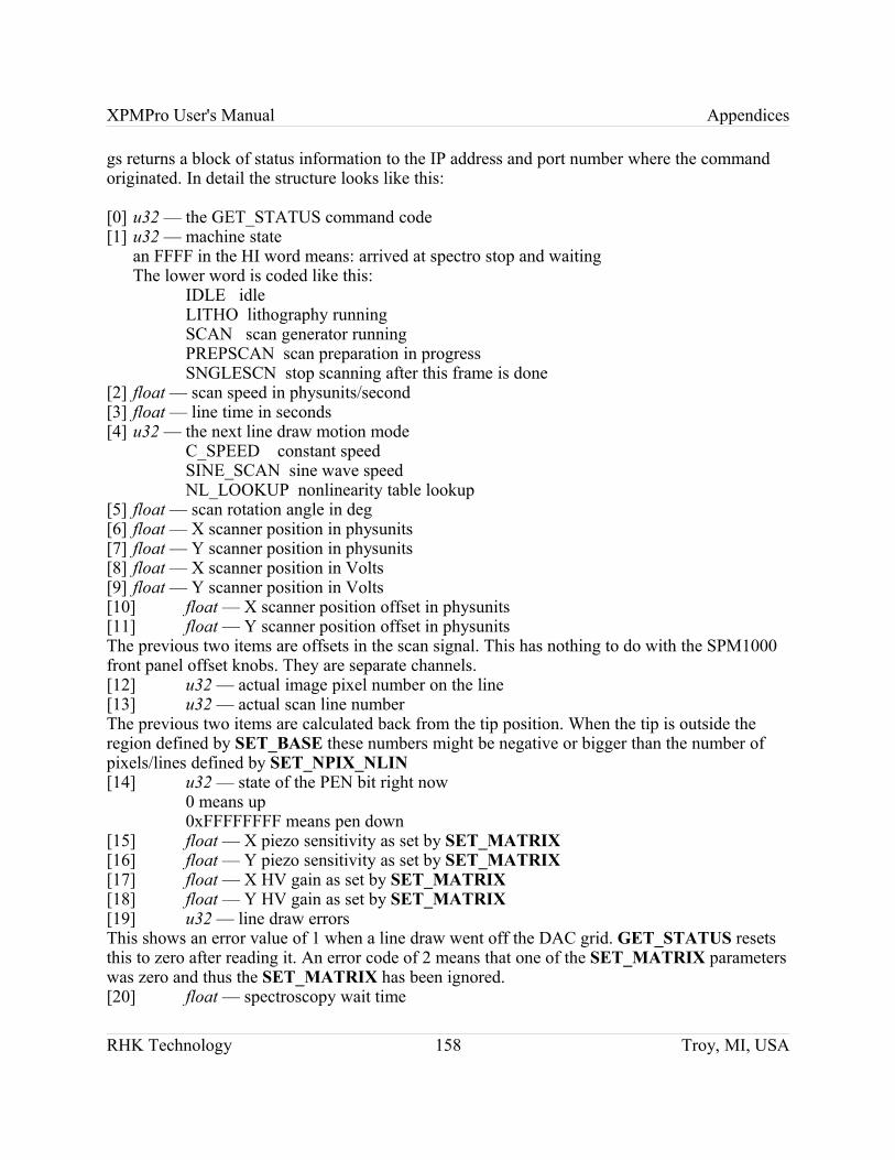
XPMPro User's Manual Appendices
gs returns a block of status information to the IP address and port number where the command originated. In detail the structure looks like this:
[0] u32 — the GET_STATUS command code [1] u32 — machine state
an FFFF in the HI word means: arrived at spectro stop and waiting The lower word is coded like this:
IDLE idleLITHO lithography runningSCAN scan generator runningPREPSCAN scan preparation in progressSNGLESCN stop scanning after this frame is done
[2] float — scan speed in physunits/second [3] float — line time in seconds [4] u32 — the next line draw motion mode
C_SPEED constant speedSINE_SCAN sine wave speedNL_LOOKUP nonlinearity table lookup
[5] float — scan rotation angle in deg [6] float — X scanner position in physunits [7] float — Y scanner position in physunits [8] float — X scanner position in Volts [9] float — Y scanner position in Volts [10] float — X scanner position offset in physunits[11] float — Y scanner position offset in physunitsThe previous two items are offsets in the scan signal. This has nothing to do with the SPM1000 front panel offset knobs. They are separate channels. [12] u32 — actual image pixel number on the line [13] u32 — actual scan line number The previous two items are calculated back from the tip position. When the tip is outside the region defined by SET_BASE these numbers might be negative or bigger than the number of pixels/lines defined by SET_NPIX_NLIN[14] u32 — state of the PEN bit right now
0 means up0xFFFFFFFF means pen down
[15] float — X piezo sensitivity as set by SET_MATRIX[16] float — Y piezo sensitivity as set by SET_MATRIX[17] float — X HV gain as set by SET_MATRIX[18] float — Y HV gain as set by SET_MATRIX[19] u32 — line draw errorsThis shows an error value of 1 when a line draw went off the DAC grid. GET_STATUS resets this to zero after reading it. An error code of 2 means that one of the SET_MATRIX parameters was zero and thus the SET_MATRIX has been ignored.[20] float — spectroscopy wait time
RHK Technology 158 Troy, MI, USA
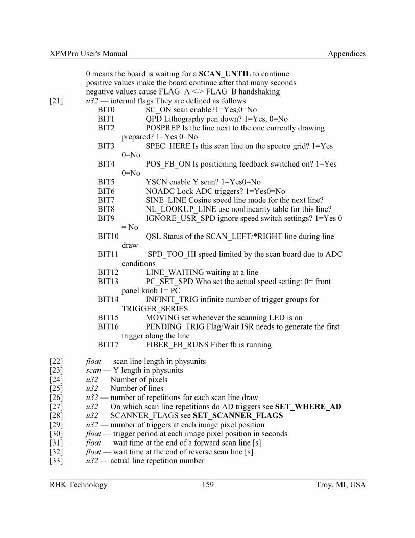
XPMPro User's Manual Appendices
0 means the board is waiting for a SCAN_UNTIL to continuepositive values make the board continue after that many secondsnegative values cause FLAG_A <-> FLAG_B handshaking
[21] u32 — internal flags They are defined as followsBIT0 SC_ON scan enable?1=Yes,0=NoBIT1 QPD Lithography pen down? 1=Yes, 0=NoBIT2 POSPREP Is the line next to the one currently drawing
prepared? 1=Yes 0=NoBIT3 SPEC_HERE Is this scan line on the spectro grid? 1=Yes
0=NoBIT4 POS_FB_ON Is positioning feedback switched on? 1=Yes
0=NoBIT5 YSCN enable Y scan? 1=Yes0=NoBIT6 NOADC Lock ADC triggers? 1=Yes0=NoBIT7 SINE_LINE Cosine speed line mode for the next line?BIT8 NL_LOOKUP_LINE use nonlinearity table for this line?BIT9 IGNORE_USR_SPD ignore speed switch settings? 1=Yes 0
= NoBIT10 QSL Status of the SCAN_LEFT/*RIGHT line during line
drawBIT11 SPD_TOO_HI speed limited by the scan board due to ADC
conditionsBIT12 LINE_WAITING waiting at a lineBIT13 PC_SET_SPD Who set the actual speed setting: 0= front
panel knob 1= PCBIT14 INFINIT_TRIG infinite number of trigger groups for
TRIGGER_SERIESBIT15 MOVING set whenever the scanning LED is onBIT16 PENDING_TRIG Flag/Wait ISR needs to generate the first
trigger along the lineBIT17 FIBER_FB_RUNS Fiber fb is running
[22] float — scan line length in physunits [23] scan — Y length in physunits [24] u32 — Number of pixels[25] u32 — Number of lines [26] u32 — number of repetitions for each scan line draw[27] u32 — On which scan line repetitions do AD triggers see SET_WHERE_AD[28] u32 — SCANNER_FLAGS see SET_SCANNER_FLAGS [29] u32 — number of triggers at each image pixel position[30] float — trigger period at each image pixel position in seconds [31] float — wait time at the end of a forward scan line [s][32] float — wait time at the end of reverse scan line [s][33] u32 — actual line repetition number
RHK Technology 159 Troy, MI, USA
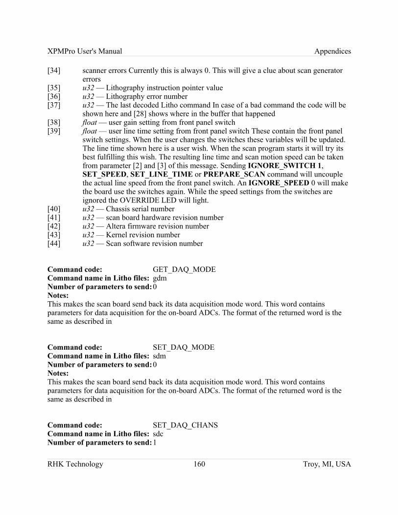
XPMPro User's Manual Appendices
[34] scanner errors Currently this is always 0. This will give a clue about scan generator errors
[35] u32 — Lithography instruction pointer value [36] u32 — Lithography error number [37] u32 — The last decoded Litho command In case of a bad command the code will be
shown here and [28] shows where in the buffer that happened[38] float — user gain setting from front panel switch [39] float — user line time setting from front panel switch These contain the front panel
switch settings. When the user changes the switches these variables will be updated. The line time shown here is a user wish. When the scan program starts it will try its best fulfilling this wish. The resulting line time and scan motion speed can be taken from parameter [2] and [3] of this message. Sending IGNORE_SWITCH 1, SET_SPEED, SET_LINE_TIME or PREPARE_SCAN command will uncouple the actual line speed from the front panel switch. An IGNORE_SPEED 0 will make the board use the switches again. While the speed settings from the switches are ignored the OVERRIDE LED will light.
[40] u32 — Chassis serial number [41] u32 — scan board hardware revision number[42] u32 — Altera firmware revision number [43] u32 — Kernel revision number [44] u32 — Scan software revision number
Command code: GET_DAQ_MODE Command name in Litho files: gdmNumber of parameters to send:0Notes:This makes the scan board send back its data acquisition mode word. This word contains parameters for data acquisition for the on-board ADCs. The format of the returned word is the same as described in
Command code: SET_DAQ_MODE Command name in Litho files: sdmNumber of parameters to send:0Notes:This makes the scan board send back its data acquisition mode word. This word contains parameters for data acquisition for the on-board ADCs. The format of the returned word is the same as described in
Command code: SET_DAQ_CHANS Command name in Litho files: sdcNumber of parameters to send:1
RHK Technology 160 Troy, MI, USA
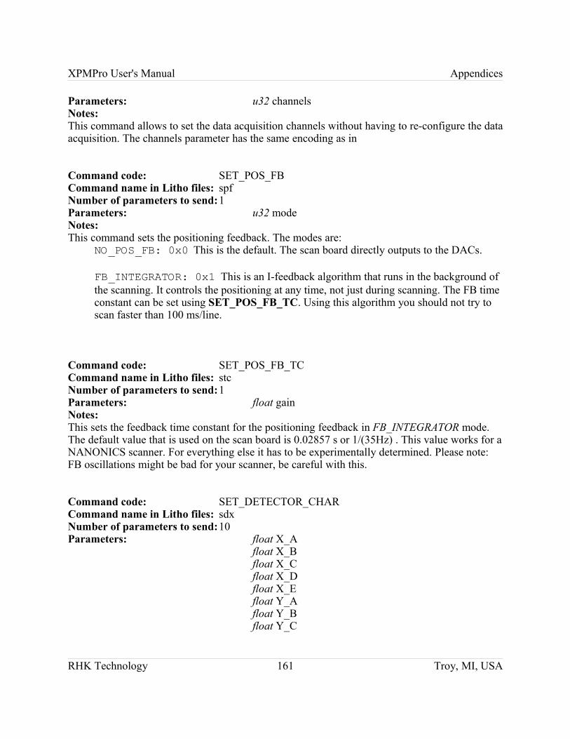
XPMPro User's Manual Appendices
Parameters: u32 channelsNotes:This command allows to set the data acquisition channels without having to re-configure the data acquisition. The channels parameter has the same encoding as in
Command code: SET_POS_FB Command name in Litho files: spfNumber of parameters to send:1Parameters: u32 modeNotes:This command sets the positioning feedback. The modes are:
NO_POS_FB: 0x0 This is the default. The scan board directly outputs to the DACs.
FB_INTEGRATOR: 0x1 This is an I-feedback algorithm that runs in the background of the scanning. It controls the positioning at any time, not just during scanning. The FB time constant can be set using SET_POS_FB_TC. Using this algorithm you should not try to scan faster than 100 ms/line.
Command code: SET_POS_FB_TC Command name in Litho files: stcNumber of parameters to send:1Parameters: float gainNotes:This sets the feedback time constant for the positioning feedback in FB_INTEGRATOR mode. The default value that is used on the scan board is 0.02857 s or 1/(35Hz) . This value works for a NANONICS scanner. For everything else it has to be experimentally determined. Please note: FB oscillations might be bad for your scanner, be careful with this.
Command code: SET_DETECTOR_CHARCommand name in Litho files: sdxNumber of parameters to send:10Parameters: float X_A
float X_Bfloat X_Cfloat X_Dfloat X_Efloat Y_Afloat Y_Bfloat Y_C
RHK Technology 161 Troy, MI, USA
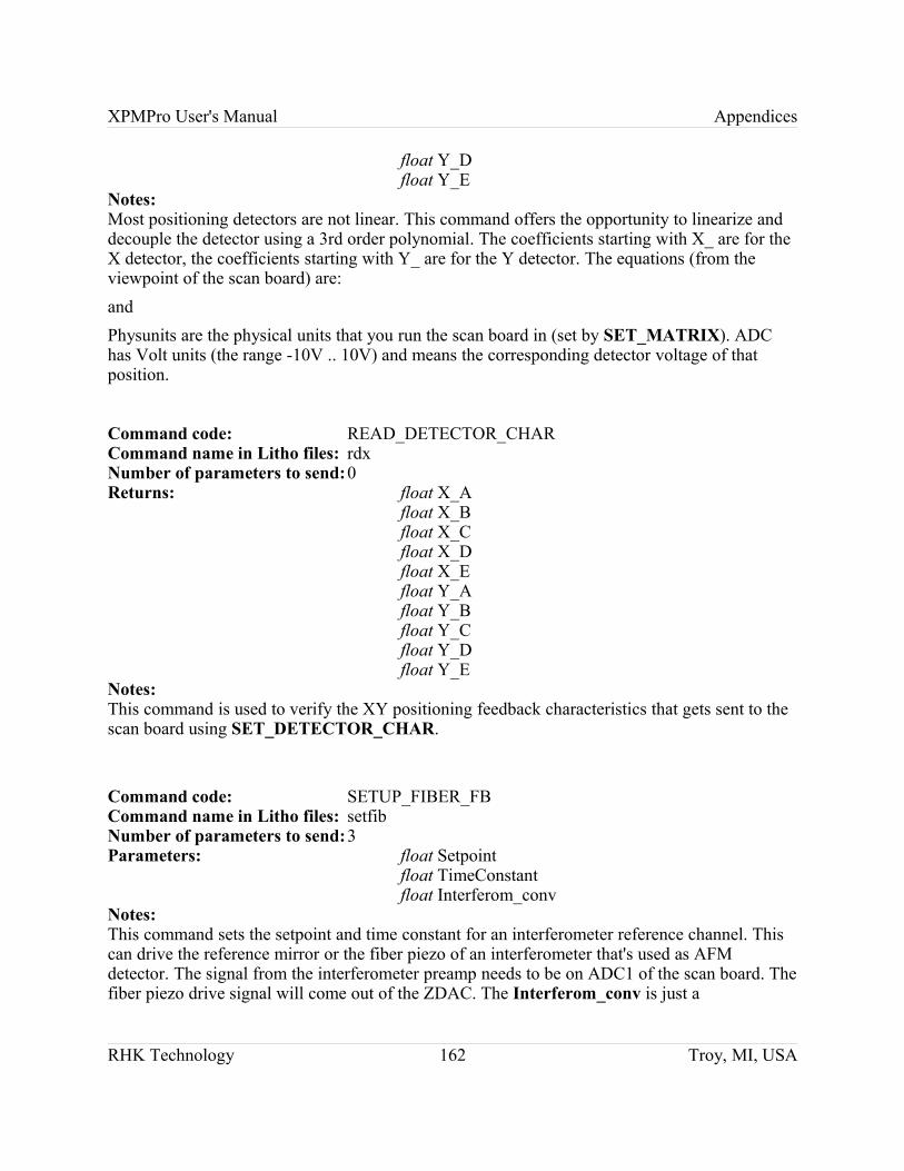
XPMPro User's Manual Appendices
float Y_Dfloat Y_E
Notes:Most positioning detectors are not linear. This command offers the opportunity to linearize and decouple the detector using a 3rd order polynomial. The coefficients starting with X_ are for the X detector, the coefficients starting with Y_ are for the Y detector. The equations (from the viewpoint of the scan board) are: and Physunits are the physical units that you run the scan board in (set by SET_MATRIX). ADC has Volt units (the range -10V .. 10V) and means the corresponding detector voltage of that position.
Command code: READ_DETECTOR_CHARCommand name in Litho files: rdxNumber of parameters to send:0Returns: float X_A
float X_Bfloat X_Cfloat X_Dfloat X_Efloat Y_Afloat Y_Bfloat Y_Cfloat Y_Dfloat Y_E
Notes:This command is used to verify the XY positioning feedback characteristics that gets sent to the scan board using SET_DETECTOR_CHAR.
Command code: SETUP_FIBER_FBCommand name in Litho files: setfibNumber of parameters to send:3Parameters: float Setpoint
float TimeConstantfloat Interferom_conv
Notes:This command sets the setpoint and time constant for an interferometer reference channel. This can drive the reference mirror or the fiber piezo of an interferometer that's used as AFM detector. The signal from the interferometer preamp needs to be on ADC1 of the scan board. The fiber piezo drive signal will come out of the ZDAC. The Interferom_conv is just a
RHK Technology 162 Troy, MI, USA
XPMPro User's Manual Appendices
configuration parameter that gets stored on the scan board. It is not used in any internal calculations but output in the GET_STATUS reply so that SPM32 can have access to this number.
Command code: START_FIBER_FBCommand name in Litho files: strtfibNumber of parameters to send:1Parameters: u32 flagNotes:This command starts or stops the fiber feedback algorithm with the parameters set up in SETUP_FIBER_FB. A value of zero in the parameter FLAG will stop the feedback. Everything else starts the feedback.
Command code: SETUP_WATCHDOGCommand name in Litho files: setwdNumber of parameters to send:3Parameters: float lowerlimit
float upperlimitBOOLEAN use_pen_line
Notes:This command sets the lower and upper limits for a signal watchdog that checks the DSP ADC2 while the fiber feedback runs. The unit for these parameters is Volts. When lowerlimit is smaller than upperlimit the watchdog checks whether the signal on DSP ADC2 is bigger than lowerlimit and smaller than upperlimit. When lowerlimit is bigger than upperlimit the algorithm checks whether the signal is bigger than lowerlimit or smaller than upperlimit. In other words: one way it tests whether the signal is within the range and the other way it tests whether the signal is outside the range. When the test fails and use_pen_line is not zero the pen_bit on the DB15 connector goes HI. The algorithm resets the pen_bit when the signal gets back into range. Also the scanner errors field (field 34) of the GET_STATUS reply will show a 1. Reading the status resets this error field.
Command code: SHOW_WATCHDOGCommand name in Litho files: showwdNumber of parameters to send:0Notes:This command displays the upper and lower limit of the signal watchdog algorithm. This will return : float lower_limit float upper_limit BOOLEAN use_pen_line
Command code: SET DRIFT RATE
RHK Technology 163 Troy, MI, USA
XPMPro User's Manual Appendices
Command name in Litho files: sdrNumber of parameters to send: 2Parameters: float Xrate
float YrateExamples: 0.01 0.01 sdrNotes: This command starts the automatic drift correction algorithm. The digital offsets of the scan board are moved at the specified rates, given in physical units. If both Xrate and Yrate are zero then the drift correction algorithm is switched off. The offsets can be returned using the SET OFFSET command even while the drift correction is active
Line draw operation commands
Command code: POSITION_ABSOLUTECommand name in Litho files: paNumber of parameters to send:2Parameters: float X
float YExamples: pa 20.0 20.0Notes:For this to work in physical units the sensitivities using SET_MATRIX must be set.
Command code: POSITION_RELATIVECommand name in Litho files: prNumber of parameters to send:2Parameters: float X
float YExamples: pr 20.0 20.0Notes:For this to work in physical units the sensitivities using SET_MATRIX must be set.
Command code: POSITION_PURECommand name in Litho files: ppNumber of parameters to send:2Parameters: float X
float YExamples: pp 20.0 20.0
RHK Technology 164 Troy, MI, USA
XPMPro User's Manual Appendices
Notes:This moves the scanner to the position (X,Y) on the unrotated and un-offset coordinate system. It is mainly used by SPM32 for range checking. X and Y are given in physical units.
Command code: POSITION_ABS_EXTDCommand name in Litho files: paeNumber of parameters to send:11Parameters: float X float Y
float speedfloat wait_time: Wait time at line end u32 flags:
Bit1 PU/PD: 0 — PU 1 — PD, Bit7 ADC: 0 — YES 1 — NO
Bit11 SCAN_LEFT DIO: 0=LOW 1=HI u32 TRIGNUM: # AD triggers at each
positionfloat TR_PERIOD: trigger period in
seconds (a pretty small number...)
u32 MotionMode: C_SPEED, SINE_SCAN or
NL_LOOKUPu32 first_Ints/AD: where first AD
u32 other_Ints/AD: AD trig separationi32 firstspec : first spectro stop after how
many A/D position updates0 — never stop, don't use remainder of previous line -1 — use remainder of counts from previous line
Examples: pae 20.0 20.0 120000.0 0.01 129 3 0.000001 0
3 5 0Notes:This function is called by the scan generator. It is the general interface of the line draw section of the program. Using this an external scan generator could take over the control of the board. Please note that the X and Y are in internal scan grid units here.
Command code: SET_WAIT_TIMECommand name in Litho files: swt
RHK Technology 165 Troy, MI, USA
XPMPro User's Manual Appendices
Number of parameters to send: 1Parameters: float wait timeExamples: swt 0.2 -> 200ms wait at line draw ends swt 0.0 -> no additional wait at line endsNotes:Internally this function gets called by POSITION_ABS_EXTD. A negative wait time results in FLAG_A being set at the end of each line. Drawing continues when FLAG_B is set. Note that the scanner sets this parameter internally. Use SET_FORWARD_WAIT_TIME and SET_REVERSE_WAIT_TIME when scanning.
Command code: SET_LINE_FLAGSCommand name in Litho files: slfNumber of parameters to send: 1Parameters: u32 flagsNotes:Internally this function gets called by POSITION_ABS_EXTD. See the POSITION_ABS_EXTD description for more details on the flags.
Command code: SET_TRIGNUMCommand name in Litho files: stnumNumber of parameters to send: 1Parameters: u32 TRIGNUM
float TRIG_PERIODNotes:This sets the number of triggers at each A/D position along the next lines. Do not use this for setting the number of triggers for the next scan. Use SET_SC_TRIGNUM instead. Internally this function gets called by POSITION_ABS_EXTD. TRIG_PERIOD is the time between trigger events in seconds
Command code: SET_MOTION_MODECommand name in Litho files: smmodNumber of parameters to send: 1Parameters: u32 motion_modeNotes:Internally this function gets called by POSITION_ABS_EXTD. It sets the motion mode for the next line to be drawn.
Command code: SET_FIRST_INTS_ADCommand name in Litho files: sfiadNumber of parameters to send: 1
RHK Technology 166 Troy, MI, USA
XPMPro User's Manual Appendices
Parameters: u32 first Ints/ADNotes:This function sets the number of scanner position updates along the line before the first A/D trigger sequence is generated. Internally this function gets called by POSITION_ABS_EXTD.
Command code: SET_OTHER_INTS_ADCommand name in Litho files: soiadNumber of parameters to send:1Parameters: u32 other_Ints/ADNotes:This function sets the number of scanner position updates along the line between all other A/D trigger positions. Internally this function gets called by POSITION_ABS_EXTD.
Command code: PEN_UPCommand name in Litho files: puNumber of parameters to send:0Notes:This will deactivate the PEN TTL output. Note that this does not happen until the beginning of the next line draw.
Command code: PEN_DOWNCommand name in Litho files: pdNumber of parameters to send:0Notes:This will activate the PEN TTL output. Note that this does not happen until the beginning of the next line draw.
Command code: ROTATE_ABSOLUTECommand name in Litho files: raNumber of parameters to send:1Parameters: float angleExamples: ra 32.31 — rotation angle = 32.31 degree Notes:This sets the rotation angle of the image coordinate system with respect to the piezo coordinate system. A positive angle means image rotation counterclockwise. The angle is given in degree. This applies to all subsequent line draw actions including scanning.
Command code: ROTATE_RELATIVECommand name in Litho files: rrNumber of parameters to send:1
RHK Technology 167 Troy, MI, USA
XPMPro User's Manual Appendices
Parameters: float angle_changeExamples: rr 0.2 — rotate drawing ccw an additonal 0.2 degree Notes:This modifies the rotation angle of the image coordinate system with respect to the piezo coordinate system. A positive angle means image rotation counterclockwise. The angle is given in degree. This applies to all subsequent line draw actions including scanning.
Command code: SET_SPEEDCommand name in Litho files: ssNumber of parameters to send:1Parameters: float speed ( in physunits/s )Notes:Internally this function gets called by POSITION_ABS_EXTD. Speed changes apply to all subsequent line draws. Note that giving a line time in PREPARE_SCAN will overwrite the speed setting.
Command code: SET MATRIX5Command name in Litho files: sm5Number of parameters to send: 5Parameters: float SkewAngle
float X Piezo sensfloat Y Piezo sensfloat HV Gain Xfloat HV Gain Y
Examples: 13.0 13.0 300.0 300.0 90 sm5Notes:This defines the meaning of physunits to the board. The piezo sensitivities are given in physunits/V, the HV Gains are dimensionless. All other operations are based on physunits so probably this is one of the first instructions given to the board. The parameter SkewAngle specifies the angle between the X and Y piezo motion in degrees. In normal microscopes this angle should be close to 90 degrees.
Command code: SET_MATRIXCommand name in Litho files: smNumber of parameters to send:4Parameters: float X_Piezo_sens float Y_Piezo_sens float HV_Gain_X
RHK Technology 168 Troy, MI, USA
XPMPro User's Manual Appendices
float HV_Gain_Y Examples: sm 300.0 300.0 13.0 13.0 Notes:This defines the meaning of "physunits" to the board. The piezo sensitivities are given in physunits/V, the HV_Gains are dimensionless. All other operations are based on physunits so this should be one of the first instructions given to the board.
Command code: SET_OFFSETCommand name in Litho files: soNumber of parameters to send:2Parameters: float Xoffs float YoffsExamples: so 20.0 -30.0Notes:This moves the offset of the scan board. The offset coordinates are given in the unrotated coordinate system (offset moves the center of rotation). Please note: changing the offset also changes the offset for the current position. The result will be a line draw to the current position at the new offset. This line draw will be done using the current line parameters.
Command code: SET OFFSET RELCommand name in Litho files: sorNumber of parameters to send: 2Parameters: float deltaXoffs
float deltaYoffsExamples: -30.0 20.0 soNotes:This moves the offset of the line draw coordinate system in respect to the piezo coordinate system. The offset coordinates are given in the unrotated coordinate system (offset moves the center of rotation) relative to the current offset position. Please note: changing the offset also changes the offset for the current position. The result will be a line draw to the current position at the new offset. This line draw will be done using the current line parameters
Command code: SET_SPEC_WAIT_TIMECommand name in Litho files: sswtNumber of parameters to send:1Parameters: float spectro_wait_timeNotes:This determines the wait time at each spectro position in table as well as in array mode. At a
RHK Technology 169 Troy, MI, USA

XPMPro User's Manual Appendices
spectro position FLAG_A is set. When the time expires, FLAG_A is cleared automatically for positive wait times. For negative wait times FLAG_B has to be put high in order to make the scanner continue.
Command code: GET_TESTCommand name in Litho files: debugNumber of parameters to send:0Notes:This command returns an array of debugging information. This array can be filled with debugging information. If unused all elements are zero.
Command code: TRIGGER_SERIESCommand name in Litho files: trsNumber of parameters to send:2Parameters: float GROUP_PERIOD
float TRIG_PERIOD u32 NGROUP u32 TRIG_NUM
Examples: trs 100e-6 10e-6 6 3This will generate 6 trigger groups each containing 3 trigger pulses 1 ms apart. The trigger pulse groups will have a period of 100 ms.Notes:This command generates a sequence of trigger groups. GROUP_PERIOD defines the period time of the trigger groups. NGROUP defines the number of groups. If this is zero triggers will be generated until told to stop by STOP_SCAN 2. TR_NUM is the number of triggers in each group. TRIG_PERIOD is the trigger period inside the group.
Command code: DRAW_ARCCommand name in Litho files: arcNumber of parameters to send:3Parameters: float X0
float Y0 float angle
Notes:This command draws an arc starting from the current position around the center point (X0,Y0). The length is determined by the given angle. Negative angle means clockwise.
Command code: DRAW_ARC_RELCommand name in Litho files: arcrNumber of parameters to send:3
RHK Technology 170 Troy, MI, USA

XPMPro User's Manual Appendices
Parameters: float X0 float Y0 float angle
Notes:This command draws an arc starting from the current position around the center point (X+dX0,Y+dY0). The coordinates of the center point are given relative to the current position. The length is determined by the given angle. Negative angle means clockwise.
Command code: SET_ANGLE_INCREMENTCommand name in Litho files: saiNumber of parameters to send:1Parameters: float angle_incrementNotes:This allows to set the angle that the arc command connects with a straight line. The default value is 1 degree. Decreasing the value makes arcs smoother but a little slower.
Command code: SHAKE_HANDCommand name in Litho files: shNumber of parameters to send:2Parameters: u32 mode
float wait_timeNotes:This allows to put wait times and handshake events into lithography files. For mode = 0 or mode = 1 a positive wait_time will be interpreted as a wait time. For mode = 2 the wait time is ignored. A negative wait_time will cause handshaking. The handshaking depends on the mode that has been set:
mode = 0 FLAG_A/FLAG_B handshake (TTL lines )mode = 1 the command suspends until a SHAKE_HAND command
with mode=2 gets sentmode = 2 The line draw gets continued
Combined with the positive or negative values that are allowed for wait_time, there are six possible circumstances that can be executed. They are:Mode=0 and positive wait_time wait for wait_timeMode=0 and negative wait_time Use FlagA/FlagB methodMode=1 and positive wait_time wait for wait_timeMode=1 and negative wait_time ethernet handshake (wait for
SHAKE_HAND with mode=2)Mode=2 and positive wait_time continue drawingMode=2 and negative wait_time continue drawingFor mode=1 and a negative wait time no UDP packet gets sent. If that is required a GET_STATUS command needs to be placed in front of this instruction in the litho file.
RHK Technology 171 Troy, MI, USA
XPMPro User's Manual Appendices
Command code: TRACK_FEATURECommand name in Litho files: tfNumber of parameters to send:1Parameters: u32 ON_OFFNotes:This starts or stops a feature tracking as set up with SETUP_TRACKING. The word ON_OFF can have these values: 0 -> shut off feature tracking 1 -> start feature tracking
Command code: SETUP_TRACKINGCommand name in Litho files: sftNumber of parameters to send:10Parameters: u32 mode
u32 nconv float Circle_Radiusfloat Circle_Freq float TimeConstant float ConeHeight float PhaseShift float Wait_Time u32 circles/trace_sample u32 not_touch_trace
Notes:This command sets up the feature tracking. In order to start feature tracking mode use the command TRACK_FEATURE. The feature tracking algorithm draws a circle of radius Circle_Radius around the current position and calculates the slope in X and in Y direction using nconv A/D conversions along the circle circumference. Assuming that the feature is a cone of height ConeHeight and that the circle radius is chosen in way that the circle is at half the cone height it calculates an X and Y displacement of the cone center with respect to the circle center. That X and Y displacement is then used to re-position the circle center on top of the cone using an integrator with the time constant TimeConstant. The cone height can be negative. In that case the algorithm tracks a depression in the surface. The mode word contains the number of circles to be drawn in the lower 16 bits. If this number is zero the algorithm circles until told to stop by a TRACK_FEATURE command. Bit 16 of the mode word determines whether SET_OFFSET ( bit 16 ==1 ) or the POSITION_ABSOLUTE (bit 16 == 0) commands are used to re-position the circle center on top of the feature. The nconv word contains the number of A/D conversions taken along each circle. This number has to be >= 3, otherwise it will get coerced to 3 by the scan board processor. The Circle_Radius is given in physical units as defined using SET_MATRIX. Circle_Freq is the number of circles drawn per second. The TimeConstant is the Feedback integrator time constant given in seconds. For a stable feedback the relation TimeConstant >= 1/Circle_Freq should be maintained. PhaseShift gives the phase shift between reference and detected signal. This way for fast
RHK Technology 172 Troy, MI, USA
XPMPro User's Manual Appendices
tracking the phase shift that is induced by the scanner mechanics can be compensated for. Wait_Time defines a wait time (in seconds) before each circle gets drawn. When the parameter not_touch_trace is set to a value different from zero this command will not configure ( and thus not reset ) the tracking trace buffer in external memory. This allows to re-configure the feature tracking without having to pick up the data of a previous run. Using an unconfigured tracking buffer means crashing the DSP board.
Command code: GET_TRACKING_DATACommand name in Litho files: gtdNumber of parameters to send:1Parameters: u32 how_manyNotes:This command reads the feature tracking trace out of the scan board external memory. It works exactly the same as READ_ADC_BUFFER except that the data that is sent back is in 32 bits IEEE float format.
Command code: PUSH_SCALECommand name in Litho files: pushsNumber of parameters to send:1Parameters: float new_scale_factorNotes:This command scales the subsequent offset and drawing operations using new_scale_factor. The factor new_scale_factor also gets put onto a 16 entries deep stack that stores the 15 previous pushs scaling factors. When more than 16 pushs operations are done without clearing the stack the first factor will get lost first.
Command code: POP_SCALECommand name in Litho files: popsNumber of parameters to send:0Notes:This command pops the scaling stack (puts the second entry into the first position etc... ) This way the scaling of a previous pushs can be restored. At initialization the scaling factor is 1.0. When the stack gets underflown it will "produce" scale factors of 1.0.
Command code: DUMP_SCALING_STACKCommand name in Litho files: dumpsNumber of parameters to send:0Notes:This command returns the contents of the scaling stack
RHK Technology 173 Troy, MI, USA

XPMPro User's Manual Appendices
Command code: SET_REPLAY_MODECommand name in Litho files: srmNumber of parameters to send:1Parameters: u32 on/offNotes:This command enables (on/off <>0) or disables (on/off=0) the replay mode. In replay mode the line draw subsystem outputs a data stream out of the A/D buffers on the Z DAC while scanning. This can be used for raster lithography along scan lines. The data can be placed into the A/D buffers with the wadc command. The buffer gets read one reading per A/D trigger that is generated by the line draw.
Command code: SET_REPLAY_FACTORCommand name in Litho files: srfNumber of parameters to send:1Parameters: float replay_factorNotes:This command sets the scale factor that gets multiplied into the ZDAC output signal in Replay Mode
Command code: SET DT TRIG PWIDTHCommand name in Litho files: sdtpwNumber of parameters to send: 1Parameters: pulse lengthNotes: This command sets the length in seconds of the trigger pulses that get sent to the DT data acquisition board in the PC. Please note that the maximum trigger period that can be set in [prepscan], page 29 or [sctnum], page 31 is twice the number given in “pulse length”.
Command code: LS_LITHO_MODECommand name in Litho files: lslmNumber of parameters to send:1Parameters: u32 on/offNotes:This command enables (on/off <>0) or disables (on/off = 0) the line start lithography mode. In this mode the lithography buffer is executed at the beginning of a line draw when a wait time <> 0 is defined.
RHK Technology 174 Troy, MI, USA
XPMPro User's Manual Appendices
Scan layer commands
Command code: PREPARE_SCANCommand name in Litho files: prepscanNumber of parameters to send:13Parameters: float baselen scan line length in physunits float basewidth — scan area height in physunits float LineTime — scan line draw time (one
way!) float fwd_wait_tm — stop time after end
of fwd line float rev_wait_tm — stop time after end
of rev line u32 npix — number of image pixels on
each line u32 nlin — number of lines in the scan u32 motionmode — C_SPEED/
SINE_SCAN/ NL_LOOKUP
u32 rept — # of repetitions for each scan line
u32 where_AD — A/D triggers on which repetitions
u32 SCANNER_FLAGS — see commands.h for coding
u32 TRIGNUM — # of triggers at each A/D position
float TRIG_PERIOD — trigger period in seconds
Example: prepscan 12 12 0.002 0 0 200 200 0 1 3 4 1 7e-6Notes:This command sets the parameters for a scan. It then moves the tip position to the scan area corner defined in SCANNER_FLAGS from where the scan is supposed to start. The motion along this line will be the speed of the scan as set by LineTime. When the tip position arrives in the start corner the scanner waits for wait_time_at_start_position seconds before further line draws can be done. Use the SCAN_UNTIL command then to start a scan. Please note that the speed of all line draws is set to the speed that corresponds to LineTime. A Linetime of 0.0 will be ignored. The old scan speed will remain unchanged.
Command code: SET_REPETITIONSCommand name in Litho files: srepNumber of parameters to send:1
RHK Technology 175 Troy, MI, USA
XPMPro User's Manual Appendices
Parameters: u32 reptNotes:Internally this function gets called by PREPARE_SCAN. It is intended mostly for testing
Command code: SET_BASECommand name in Litho files: sbasNumber of parameters to send:2Parameters: float base_length float base_widthNotes:Internally this function gets called by PREPARE_SCAN. It is intended mostly for testing. The values base_length and base_width give the size of the scan area in physunits.
Command code: SET_LINETIMECommand name in Litho files: sltNumber of parameters to send:1Parameters: float Line_timeNotes:Internally this function gets called by PREPARE_SCAN. It sets the scan line time. The scan line time is the time that just the forward scan line would take, not a forth and back scan... When other parameters change the system tries to conserve the line time.
Command code: SET_FWD_WAIT_TIMECommand name in Litho files: sfwtNumber of parameters to send:1Parameters: float wait time at the end of a fwd line [s]Notes:Internally this function gets called by PREPARE_SCAN. It is intended mostly for testing. The time is given in seconds. Negative wait time results in FLAG_A being set at the end of each fwd line. Scanning continues when FLAG_B is set.
Command code: SET_REV_WAIT_TIMECommand name in Litho files: srwtNumber of parameters to send:1Parameters: float wait time at the end of a rev line [s] Notes:Internally this function gets called by PREPARE_SCAN. It is intended mostly for testing. The time is given in seconds. Negative wait time results in FLAG_A being set at the end of each rev line. Scanning continues when FLAG_B is set.
RHK Technology 176 Troy, MI, USA
XPMPro User's Manual Appendices
Command code: SET_NPIX_NLINCommand name in Litho files: snpNumber of parameters to send:2Parameters: u32 npix u32 nlinNotes:Internally this function gets called by PREPARE_SCAN. It is intended mostly for testing.
Command code: SET_SC_MOTMODCommand name in Litho files: smmNumber of parameters to send:1Parameters: u32 motion_modeNotes:This function sets the motion for the scan lines of all following scans. The connection lines will be constant speed lines.
Command code: SET_WHERE_ADCommand name in Litho files: swadNumber of parameters to send:1Parameters: u32 where_ADNotes:Internally this function gets called by PREPARE_SCAN. It is intended mostly for testing. In where_AD each bit allows AD trigger generation on a certain line repetition number. Bit 0 means first fwd line, bit 1 means 1st rev line etc. A value of where_AD of 2 means only generate A/D trigger sequences at the first backward scan. The bits in here are only considered when the line is drawn. That has to be set using SET_REPETITIONS.
Command code: SET_SCANNER_FLAGSCommand name in Litho files: ssfNumber of parameters to send:1Parameters: u32 SCANNER_FLAGSNotes:Internally this function gets called by PREPARE_SCAN. It is intended mostly for testing. The scanner flags describe:Start corner:
Bit 0: 1 — lower 0 — upper Bit 1: 1 — right 0 — left
Slow scan direction:Bit 2: 1 — keep 0 — alternate
RHK Technology 177 Troy, MI, USA
XPMPro User's Manual Appendices
Command code: SET_SC_TRIGNUMCommand name in Litho files: sctnumNumber of parameters to send:2Parameters: u32 TRIGNUM
float TRIG_PERIODNotes:Internally this function gets called by PREPARE_SCAN. It is intended mostly for testing. It sets the number of A/D triggers generated at each A/D position. Note that this is the value used by the scan generator. If you set TRIGNUM by using SET_TRIGNUM this will be overwritten by the SET_SC_TRIGNUM value at the begin of the next scan. TRIG_PERIOD is the time between trigger events in seconds
Command code: MOVE_TO_SCAN_STARTCommand name in Litho files: msNumber of parameters to send:0Notes:This moves the tip position to the scan area corner defined in SCANNER_FLAGS from where the scan is supposed to start. The motion along this line will be the speed of the scan as set by LineTime. Use the SCAN_UNTIL command then to start a scan. Internally this function gets called by PREPARE_SCAN after all other parameters have been set. A MOVE_TO_SCAN_START command can be issued at any time. It will then use the configurations of the last PREPARE_SCAN. When a scan is running a MOVE_TO_SCAN_START command will stop the current scan at the end of the next prepared line and then move to the start corner. Please note that the scan generator works in the background of the line draws that it has "ordered". Any line that got ordered will be drawn. This means that when you issue a MOVE_TO_SCAN_START command the scanner might actually draw another line after the current one before it responds.
Command code: SCAN_UNTILCommand name in Litho files: suNumber of parameters to send:1Parameters: u32 #image_pixelsExamples: stpsc 1 ms su 0 — stops the old and starts a new continuous
scan Notes:SCAN_UNTIL is the command to use when the scanner should move further along the scan lines. The value in #image_pixels will tell when the scan gets stopped again. A value of 0 means continuous scanning. When the scan is stopped the high word of the machine state word in the GET_STATUS reply is set to 0xffff. The low word still stays at SCAN. SCAN_UNTIL is the command to use for spectroscopy. SCAN_UNTIL is also used to get a scan running after the
RHK Technology 178 Troy, MI, USA
XPMPro User's Manual Appendices
MOVE_TO_START command. When a SCAN_UNTIL is applied to a running line draw it sets the number of A/D conversions from the moment the command came in to the next spectro stop.
Command code: STOP_SCANCommand name in Litho files: stpscNumber of parameters to send:1Parameters: u32 WHERENotes:This command is used to stop the scan in a defined way. The parameter WHERE says where to abort the scan. The coding is:EOSCAN stops at the end of a scan frame. Note that this sets the machine state to SNGLESCN
for the rest of the frameEOLN stops the scan at the end of this scan lineSTOP_NOW stops the scan immediately, aborting the current line drawAfter the STOP_SCAN command the tip position does NOT move to the start corner. You have to use MOVE_TO_SCAN_START for that. Scans stopped at EOSCAN or EOLN can be continued using SCAN_UNTIL. For a scan stopped at STOP_NOW this will give unpredictable results. Use INTERRUPT_SCAN if you want to stop at a previously unknown position along a scan line and then want to continue scanning.
Command code: INTERRUPT_SCANCommand name in Litho files: intscNumber of parameters to send:0Notes:This command forces a spectroscopy stop at the position of the scanner. Using SCAN_UNTIL the scan can be continued afterward. As on any spectro stop position the high word of the machine_state variable is set to 0xffff while the scan is interrupted.
Command code: STOP_Y_SCANCommand name in Litho files: stopyNumber of parameters to send:1Parameters: u32 YES_NO — STOP Y = 1 RUN Y = 0Notes:This sets or clears a scan generator flag which tells whether the Y line position should be changed during scanning. This allows to scan a whole image along one line. This might be interesting for testing the SPM imaging conditions.
Command code: SET_WHERE_SPECCommand name in Litho files: sws
RHK Technology 179 Troy, MI, USA
XPMPro User's Manual Appendices
Number of parameters to send:1Parameters: u32 where_spectroNotes:Each bit in where_spectro represents a line repetition during scanning. When the bit is set automatic spectroscopy is allowed on that scan repetition.
Command code: SPEC_ARRAY_MODECommand name in Litho files: samNumber of parameters to send:4Parameters: u32 first_pix,
u32 delta_pix, u32 firstlin, u32 deltalin
Notes:This switches on array mode automatic spectroscopy during the scan line repetitions set by SET_WHERE_SPEC. Please note that spectroscopy is only possible at points where A/D conversions are taken. Disabling A/D conversions along a line automatically also disables spectroscopy. The parameter first_pix gives the pixel position of the first spectroscopy position from the line start point. The parameter delta_pix gives the separation of the spectro positions along the line in A/D conversion steps. The parameter firstlin gives the first scan line that contains spectro stops, counted from the begin of the scan. The parameter deltalin gives the separation of spectro scan lines along the image. When firstlin < deltalin the spectro positions of a downward scan and the following upward scan lie exactly on top of each other.array spectro parameters are:
first_pix — (goes 0 ... npix-1)delta_pix — (minimum 1)firstlin — (goes 0 ... nlin-1)deltalin — (minimum 1)
Command code: SPEC_TABLE_MODECommand name in Litho files: stmNumber of parameters to send:depends on table lengthParameters: spectro position tableNotes:This command switches on table spectroscopy mode. This allows the placement of spectroscopy positions on any A/D trigger position on the image. The table contains line numbers (which have 0x0000 in the high word) and position markers for the spectro position on that line. The position markers are compressed. The Hi word contains a repetition counter and the lower word the position difference to the previous position or to the line start. Note that there is a position difference of 1 needed to reach position 0 on the line. A position difference of zero will shut off spectroscopy for the rest of the line. The table is coded like this:line number ( has 0x0000 in the high word)
RHK Technology 180 Troy, MI, USA
XPMPro User's Manual Appendices
entry 1, has repetition cntr in Hi word and position X difference in lo wordentry 2, has repetition cntr in Hi word and position X difference in lo wordentry 3, has repetition cntr in Hi word and position X difference in lo word...entry n, has repetition cntr in Hi word and position X difference in lo word
line number ( has 0x0000 in the high word)entry 1, has repetition cntr in Hi word and position X difference in lo wordentry 2, has repetition cntr in Hi word and position X difference in lo word...
Example:0x00x000300010x050x000200030x000100040x0c0x000300030x00020001
will place spectro stops on line 0 at positions 0, 1, and 2line 5 at A/D positions 2, 5, 9 andline 12 at A/D position 2, 5, 8, 9, 10The pixel numbers start with 0 and are in decimal notation here.
Command code: SPEC_NO_MODECommand name in Litho files: snmNumber of parameters to send:0Notes:This shuts off automatic spectroscopy. SCAN_UNTIL will still do "manual" spectro positioning.
Command code: N_LINREPCommand name in Litho files: linrepNumber of parameters to send:0Notes:This command puts the number of the line repetition of the scan generator onto the Lithography parameter stack. It can be used to make decisions in lithography files that get started at the beginning of multi line images.
RHK Technology 181 Troy, MI, USA

XPMPro User's Manual Appendices
Lithography commands
Command code: WRITE_LITHO_BUFCommand name in Litho files: wlbNumber of parameters to send:variableParameters: Instructions to be put into litho bufferNotes:This command can not be put into the lithography buffer. That does not make sense. This is the only command with a variable length. The user has to make sure that the sent packet size does not exceed the ethernet packet size. Otherwise the packet will be split up by the IP layer of the control computer and then ignored by the scan board IP routine. Longer instruction sequences can be downloaded by subsequent WRITE_LITHO_BUF instructions. After the download has succeeded the lithography pointer points to the first free memory cell after the downloaded commands. This allows multiple WRITE_LITHO_BUF commands to write more instructions than what fits into one ethernet buffer. The WRITE_LITHO_BUF instruction returns the following data structure to the IP address and UDP port number that issued the command:[0] WRITE_LITHO_BUF code[1] number of written instructions[2] remaining free spaces in litho bufferThis is mainly used to confirm that the packet arrived and got processed. (It might get lost in UDP...)
Command code: RESET_LITHO_BUFCommand name in Litho files: rlbNumber of parameters to send:0Notes:This is used to stop a running lithography sequence and to set the lithography pointer back to the begin of the buffer. Please note that the lithography buffer controls both where instructions get written to by WRITE_LITHO_BUF and where they are read from during execution.
Command code: JUMP_BUFCommand name in Litho files: jlbNumber of parameters to send:1Parameters: u32 positionExamples: jlb 0 jumps back to the begin and continuesNotes:This command simply changes the lithography pointer. This way loops are possible. Conditional jumps are not supported in this version.
Command code: DO_LITHO
RHK Technology 182 Troy, MI, USA

XPMPro User's Manual Appendices
Command name in Litho files: dlNumber of parameters to send:0Notes:This executes the commands in the lithography buffer starting at where the lithography pointer points to. During lithography execution the lower word of the machine_state word is set to LITHO.
Command code: PLUSCommand name in Litho files: +Number of parameters to send:0Notes:This command adds the two topmost entries on the Lithography stack. It can only be run from inside a Litho file.
Command code: JNZCommand name in Litho files: jnzNumber of parameters to send:0Notes:This command will execute a relative jump inside the lithography buffer. The top of the parameter stack is the offset of the jump, counted from one position behind the jnz instruction. Underneath is the counter parameter. When the counter parameter is zero it gets removed from the stack and no jump is executed. Otherwise the instruction does the relative jump. Please look at the looptest.lth example file in the C_utilities for an example of this.
RHK Technology 183 Troy, MI, USA
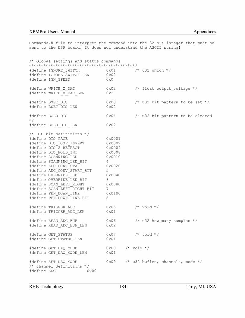
XPMPro User's Manual Appendices
Commands.h file to interpret the command into the 32 bit integer that must be sent to the DSP board. It does not understand the ASCII string!
/* Global settings and status commands ********************************************/#define IGNORE_SWITCH 0x01 /* u32 which */#define IGNORE_SWITCH_LEN 0x02#define IGN_SPEED 0x0
#define WRITE_Z_DAC 0x02 /* float output_voltage */#define WRITE_Z_DAC_LEN 0x2
#define BSET_DIO 0x03 /* u32 bit pattern to be set */#define BSET_DIO_LEN 0x02
#define BCLR_DIO 0x04 /* u32 bit pattern to be cleared */#define BCLR_DIO_LEN 0x02
/* DIO bit definitions */#define DIO_PAGE 0x0001#define DIO_LOOP_INVERT 0x0002#define DIO_Z_RETRACT 0x0004#define DIO_HOLD_INT 0x0008#define SCANNING_LED 0x0010#define SCANNING_LED_BIT 4#define ADC_CONV_START 0x0020#define ADC_CONV_START_BIT 5#define OVERRIDE_LED 0x0040#define OVERRIDE_LED_BIT 6#define SCAN_LEFT_RIGHT 0x0080#define SCAN_LEFT_RIGHT_BIT 7#define PEN_DOWN_LINE 0x0100#define PEN_DOWN_LINE_BIT 8
#define TRIGGER_ADC 0x05 /* void */#define TRIGGER_ADC_LEN 0x01
#define READ_ADC_BUF 0x06 /* u32 how_many samples */#define READ_ADC_BUF_LEN 0x02
#define GET_STATUS 0x07 /* void */#define GET_STATUS_LEN 0x01
#define GET_DAQ_MODE 0x08 /* void */#define GET_DAQ_MODE_LEN 0x01
#define SET_DAQ_MODE 0x09 /* u32 buflen, channels, mode *//* channel definitions */#define ADC1 0x00
RHK Technology 184 Troy, MI, USA
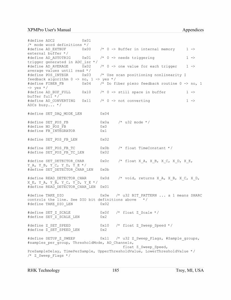
XPMPro User's Manual Appendices
#define ADC2 0x01/* mode word definitions */#define AD_EXTBUF 0x00 /* 0 -> Buffer in internal memory 1 -> external buffer */#define AD_AUTOTRIG 0x01 /* 0 -> needs triggering 1 -> trigger generated in ADC_isr */#define AD_AVERAGE 0x02 /* 0 -> one value for each trigger 1 -> average values until read */#define POS_INTEGR 0x03 /* Use scan positioning nonlinearity I feedback algorithm 0 -> no, 1 -> yes */#define FIBER_FB 0x04 /* Do fiber piezo feedback routine 0 -> no, 1 -> yes */#define AD_BUF_FULL 0x10 /* 0 -> still space in buffer 1 -> buffer full */#define AD_CONVERTING 0x11 /* 0 -> not converting 1 -> ADCs busy... */
#define SET_DAQ_MODE_LEN 0x04
#define SET_POS_FB 0x0a /* u32 mode */#define NO_POS_FB 0x0#define FB_INTEGRATOR 0x1
#define SET_POS_FB_LEN 0x02
#define SET_POS_FB_TC 0x0b /* float TimeConstant */#define SET_POS_FB_TC_LEN 0x02
#define SET_DETECTOR_CHAR 0x0c /* float X_A, X_B, X_C, X_D, X_E, Y_A, Y_B, Y_C, Y_D, Y_E */#define SET_DETECTOR_CHAR_LEN 0x0b
#define READ_DETECTOR_CHAR 0x0d /* void, returns X_A, X_B, X_C, X_D, X_E, Y_A, Y_B, Y_C, Y_D, Y_E */#define READ_DETECTOR_CHAR_LEN 0x01
#define TAKE_DIO 0x0e /* u32 BIT_PATTERN ... a 1 means SHARC controls the line. See DIO bit definitions above */#define TAKE_DIO_LEN 0x02
#define SET_Z_SCALE 0x0f /* float Z_Scale */#define SET_Z_SCALE_LEN 0x2
#define Z_SET_SPEED 0x10 /* float Z_Sweep_Speed */#define Z_SET_SPEED_LEN 0x2
#define SETUP_Z_SWEEP 0x11 /* u32 Z_Sweep_Flags, #Sample_groups, #samples_per_group, ThresholdMode, AD_Channels, float Z_Sweep_Speed, PreSampleDelay, TimePerSample, UpperThresholdValue, LowerThresholdValue *//* Z_Sweep_Flags */
RHK Technology 185 Troy, MI, USA
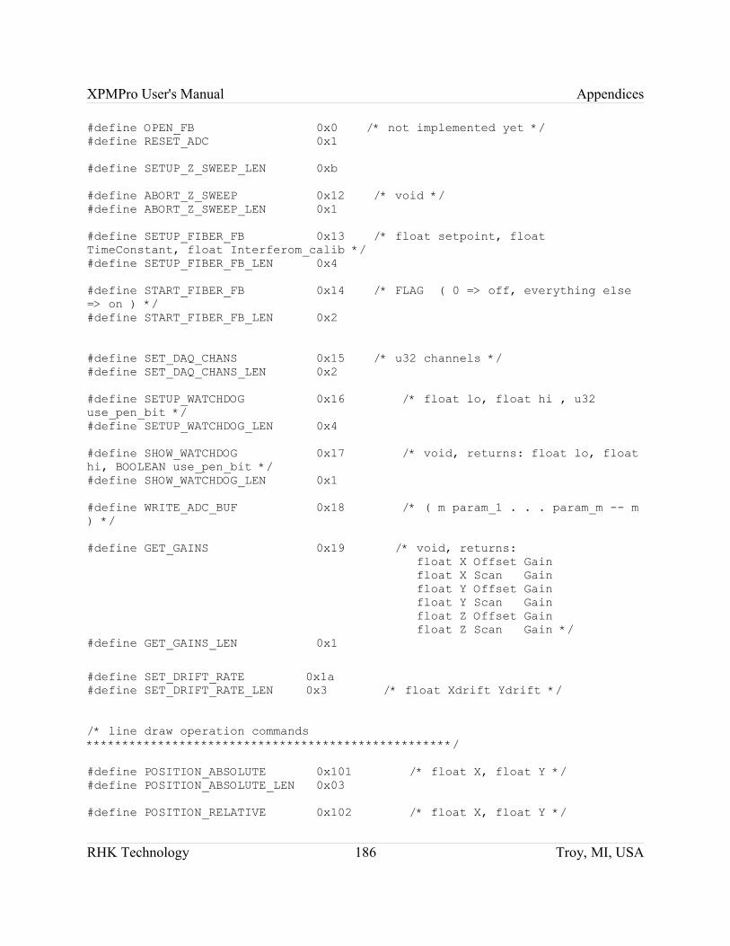
XPMPro User's Manual Appendices
#define OPEN_FB 0x0 /* not implemented yet */#define RESET_ADC 0x1
#define SETUP_Z_SWEEP_LEN 0xb
#define ABORT_Z_SWEEP 0x12 /* void */#define ABORT_Z_SWEEP_LEN 0x1
#define SETUP_FIBER_FB 0x13 /* float setpoint, float TimeConstant, float Interferom_calib */#define SETUP_FIBER_FB_LEN 0x4
#define START_FIBER_FB 0x14 /* FLAG ( 0 => off, everything else => on ) */#define START_FIBER_FB_LEN 0x2
#define SET_DAQ_CHANS 0x15 /* u32 channels */#define SET_DAQ_CHANS_LEN 0x2
#define SETUP_WATCHDOG 0x16 /* float lo, float hi , u32 use_pen_bit */#define SETUP_WATCHDOG_LEN 0x4
#define SHOW_WATCHDOG 0x17 /* void, returns: float lo, float hi, BOOLEAN use_pen_bit */#define SHOW_WATCHDOG_LEN 0x1
#define WRITE_ADC_BUF 0x18 /* ( m param_1 . . . param_m -- m ) */
#define GET_GAINS 0x19 /* void, returns: float X Offset Gain float X Scan Gain float Y Offset Gain float Y Scan Gain float Z Offset Gain float Z Scan Gain */#define GET_GAINS_LEN 0x1
#define SET_DRIFT_RATE 0x1a#define SET_DRIFT_RATE_LEN 0x3 /* float Xdrift Ydrift */
/* line draw operation commands ***************************************************/
#define POSITION_ABSOLUTE 0x101 /* float X, float Y */#define POSITION_ABSOLUTE_LEN 0x03
#define POSITION_RELATIVE 0x102 /* float X, float Y */
RHK Technology 186 Troy, MI, USA
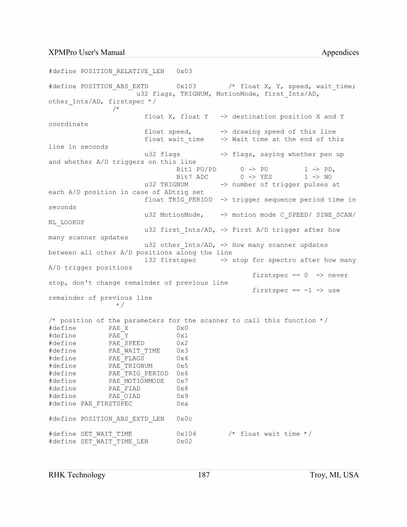
XPMPro User's Manual Appendices
#define POSITION_RELATIVE_LEN 0x03
#define POSITION_ABS_EXTD 0x103 /* float X, Y, speed, wait_time; u32 flags, TRIGNUM, MotionMode, first_Ints/AD, other_Ints/AD, firstspec */ /* float X, float Y -> destination position X and Y coordinate float speed, -> drawing speed of this line float wait_time -> Wait time at the end of this line in seconds u32 flags -> flags, saying whether pen up and whether A/D triggers on this line Bit1 PU/PD 0 -> PU 1 -> PD, Bit7 ADC 0 -> YES 1 -> NO u32 TRIGNUM -> number of trigger pulses at each A/D position in case of ADtrig set float TRIG_PERIOD -> trigger sequence period time in seconds u32 MotionMode, -> motion mode C_SPEED/ SINE_SCAN/ NL_LOOKUP u32 first_Ints/AD, -> First A/D trigger after how many scanner updates u32 other_Ints/AD, -> How many scanner updates between all other A/D positions along the line i32 firstspec -> stop for spectro after how many A/D trigger positions firstspec == 0 -> never stop, don't change remainder of previous line firstspec == -1 -> use remainder of previous line */
/* position of the parameters for the scanner to call this function */#define PAE_X 0x0#define PAE_Y 0x1#define PAE_SPEED 0x2#define PAE_WAIT_TIME 0x3#define PAE_FLAGS 0x4#define PAE_TRIGNUM 0x5#define PAE_TRIG_PERIOD 0x6#define PAE_MOTIONMODE 0x7#define PAE_FIAD 0x8#define PAE_OIAD 0x9#define PAE_FIRSTSPEC 0xa
#define POSITION_ABS_EXTD_LEN 0x0c
#define SET_WAIT_TIME 0x104 /* float wait time */#define SET_WAIT_TIME_LEN 0x02
RHK Technology 187 Troy, MI, USA
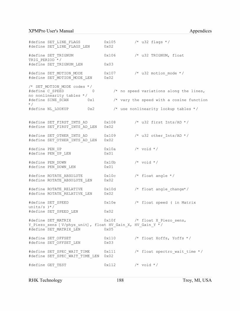
XPMPro User's Manual Appendices
#define SET_LINE_FLAGS 0x105 /* u32 flags */#define SET_LINE_FLAGS_LEN 0x02
#define SET_TRIGNUM 0x106 /* u32 TRIGNUM, float TRIG_PERIOD */#define SET_TRIGNUM_LEN 0x03
#define SET_MOTION_MODE 0x107 /* u32 motion_mode */#define SET_MOTION_MODE_LEN 0x02
/* SET_MOTION_MODE codes */#define C_SPEED 0 /* no speed variations along the lines, no nonlinearity tables */#define SINE_SCAN 0x1 /* vary the speed with a cosine function */#define NL_LOOKUP 0x2 /* use nonlinearity lookup tables */
#define SET_FIRST_INTS_AD 0x108 /* u32 first Ints/AD */#define SET_FIRST_INTS_AD_LEN 0x02
#define SET_OTHER_INTS_AD 0x109 /* u32 other_Ints/AD */#define SET_OTHER_INTS_AD_LEN 0x02
#define PEN_UP 0x10a /* void */#define PEN_UP_LEN 0x01
#define PEN_DOWN 0x10b /* void */#define PEN_DOWN_LEN 0x01
#define ROTATE_ABSOLUTE 0x10c /* float angle */#define ROTATE_ABSOLUTE_LEN 0x02
#define ROTATE_RELATIVE 0x10d /* float angle_change*/#define ROTATE_RELATIVE_LEN 0x02
#define SET_SPEED 0x10e /* float speed ( in Matrix units/s )*/#define SET_SPEED_LEN 0x02
#define SET_MATRIX 0x10f /* float X_Piezo_sens, Y_Piezo_sens [V/phys_unit], float HV_Gain_X, HV_Gain_Y */#define SET_MATRIX_LEN 0x05
#define SET_OFFSET 0x110 /* float Xoffs, Yoffs */#define SET_OFFSET_LEN 0x03
#define SET_SPEC_WAIT_TIME 0x111 /* float spectro_wait_time */#define SET_SPEC_WAIT_TIME_LEN 0x02
#define GET_TEST 0x112 /* void */
RHK Technology 188 Troy, MI, USA
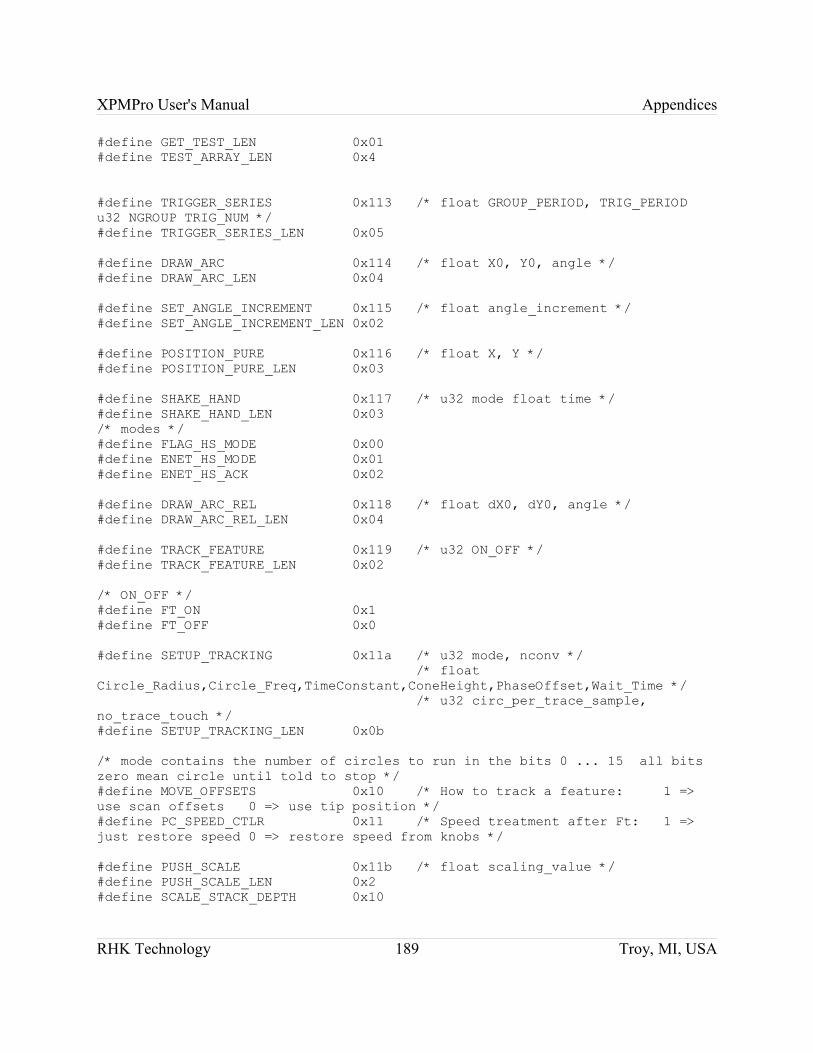
XPMPro User's Manual Appendices
#define GET_TEST_LEN 0x01 #define TEST_ARRAY_LEN 0x4
#define TRIGGER_SERIES 0x113 /* float GROUP_PERIOD, TRIG_PERIOD u32 NGROUP TRIG_NUM */ #define TRIGGER_SERIES_LEN 0x05
#define DRAW_ARC 0x114 /* float X0, Y0, angle */#define DRAW_ARC_LEN 0x04
#define SET_ANGLE_INCREMENT 0x115 /* float angle_increment */#define SET_ANGLE_INCREMENT_LEN 0x02
#define POSITION_PURE 0x116 /* float X, Y */#define POSITION_PURE_LEN 0x03
#define SHAKE_HAND 0x117 /* u32 mode float time */#define SHAKE_HAND_LEN 0x03/* modes */#define FLAG_HS_MODE 0x00#define ENET_HS_MODE 0x01#define ENET_HS_ACK 0x02
#define DRAW_ARC_REL 0x118 /* float dX0, dY0, angle */#define DRAW_ARC_REL_LEN 0x04
#define TRACK_FEATURE 0x119 /* u32 ON_OFF */#define TRACK_FEATURE_LEN 0x02
/* ON_OFF */#define FT_ON 0x1#define FT_OFF 0x0
#define SETUP_TRACKING 0x11a /* u32 mode, nconv */ /* float Circle_Radius,Circle_Freq,TimeConstant,ConeHeight,PhaseOffset,Wait_Time */ /* u32 circ_per_trace_sample, no_trace_touch */#define SETUP_TRACKING_LEN 0x0b
/* mode contains the number of circles to run in the bits 0 ... 15 all bits zero mean circle until told to stop */#define MOVE_OFFSETS 0x10 /* How to track a feature: 1 => use scan offsets 0 => use tip position */ #define PC_SPEED_CTLR 0x11 /* Speed treatment after Ft: 1 => just restore speed 0 => restore speed from knobs */
#define PUSH_SCALE 0x11b /* float scaling_value */#define PUSH_SCALE_LEN 0x2#define SCALE_STACK_DEPTH 0x10
RHK Technology 189 Troy, MI, USA
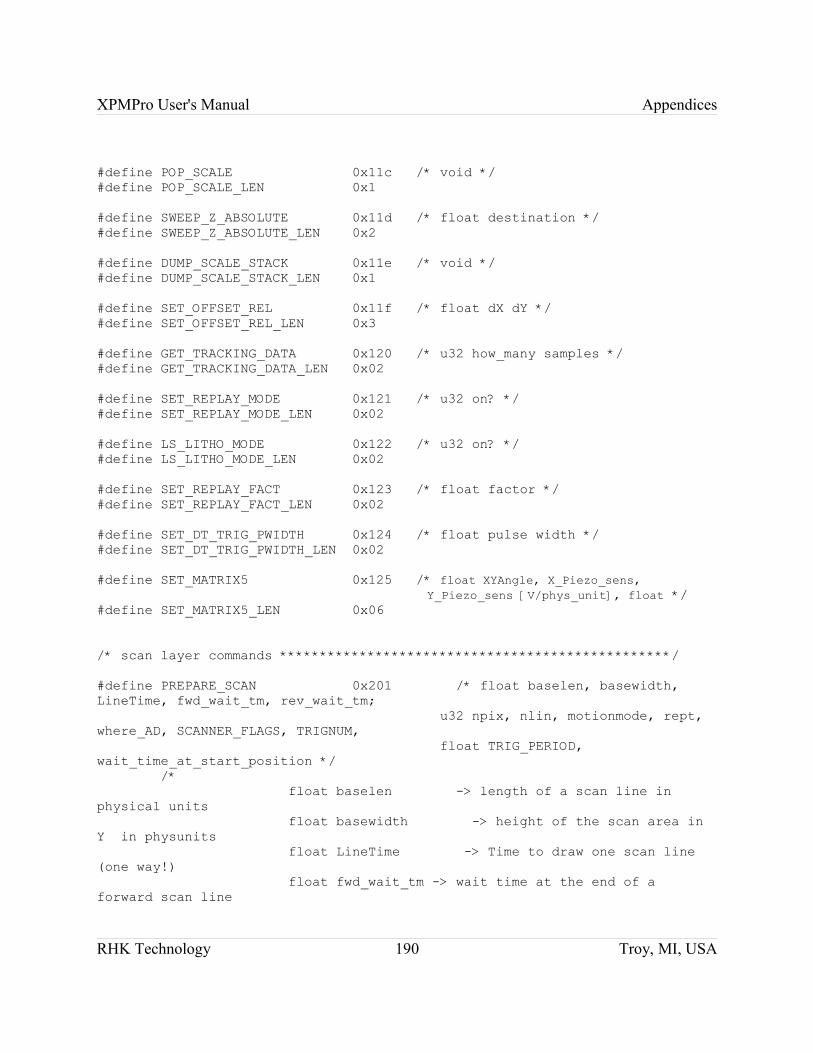
XPMPro User's Manual Appendices
#define POP_SCALE 0x11c /* void */#define POP_SCALE_LEN 0x1
#define SWEEP_Z_ABSOLUTE 0x11d /* float destination */#define SWEEP_Z_ABSOLUTE_LEN 0x2
#define DUMP_SCALE_STACK 0x11e /* void */#define DUMP_SCALE_STACK_LEN 0x1
#define SET_OFFSET_REL 0x11f /* float dX dY */#define SET_OFFSET_REL_LEN 0x3
#define GET_TRACKING_DATA 0x120 /* u32 how_many samples */#define GET_TRACKING_DATA_LEN 0x02
#define SET_REPLAY_MODE 0x121 /* u32 on? */#define SET_REPLAY_MODE_LEN 0x02
#define LS_LITHO_MODE 0x122 /* u32 on? */#define LS_LITHO_MODE_LEN 0x02
#define SET_REPLAY_FACT 0x123 /* float factor */#define SET_REPLAY_FACT_LEN 0x02
#define SET_DT_TRIG_PWIDTH 0x124 /* float pulse width */#define SET_DT_TRIG_PWIDTH_LEN 0x02
#define SET_MATRIX5 0x125 /* float XYAngle, X_Piezo_sens, Y_Piezo_sens [V/phys_unit], float */
#define SET_MATRIX5_LEN 0x06
/* scan layer commands *************************************************/
#define PREPARE_SCAN 0x201 /* float baselen, basewidth, LineTime, fwd_wait_tm, rev_wait_tm; u32 npix, nlin, motionmode, rept, where_AD, SCANNER_FLAGS, TRIGNUM, float TRIG_PERIOD, wait_time_at_start_position */ /* float baselen -> length of a scan line in physical units float basewidth -> height of the scan area in Y in physunits float LineTime -> Time to draw one scan line (one way!) float fwd_wait_tm -> wait time at the end of a forward scan line
RHK Technology 190 Troy, MI, USA
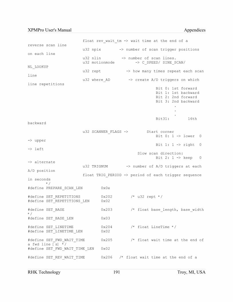
XPMPro User's Manual Appendices
float rev_wait_tm -> wait time at the end of a reverse scan line u32 npix -> number of scan trigger positions on each line u32 nlin -> number of scan lines. u32 motionmode -> C_SPEED/ SINE_SCAN/ NL_LOOKUP u32 rept -> how many times repeat each scan line u32 where_AD -> create A/D triggers on which line repetitions Bit 0: 1st forward Bit 1: 1st backward Bit 2: 2nd forward Bit 3: 2nd backward . . . Bit31: 16th backward
u32 SCANNER_FLAGS -> Start corner Bit 0: 1 -> lower 0 -> upper Bit 1: 1 -> right 0 -> left Slow scan direction: Bit 2: 1 -> keep 0 -> alternate u32 TRIGNUM -> number of A/D triggers at each A/D position float TRIG_PERIOD -> period of each trigger sequence in seconds */#define PREPARE_SCAN_LEN 0x0e
#define SET_REPETITIONS 0x202 /* u32 rept */#define SET_REPETITIONS_LEN 0x02
#define SET_BASE 0x203 /* float base_length, base_width */#define SET_BASE_LEN 0x03
#define SET_LINETIME 0x204 /* float LineTime */#define SET_LINETIME_LEN 0x02
#define SET_FWD_WAIT_TIME 0x205 /* float wait time at the end of a fwd line [s] */ #define SET_FWD_WAIT_TIME_LEN 0x02
#define SET_REV_WAIT_TIME 0x206 /* float wait time at the end of a
RHK Technology 191 Troy, MI, USA
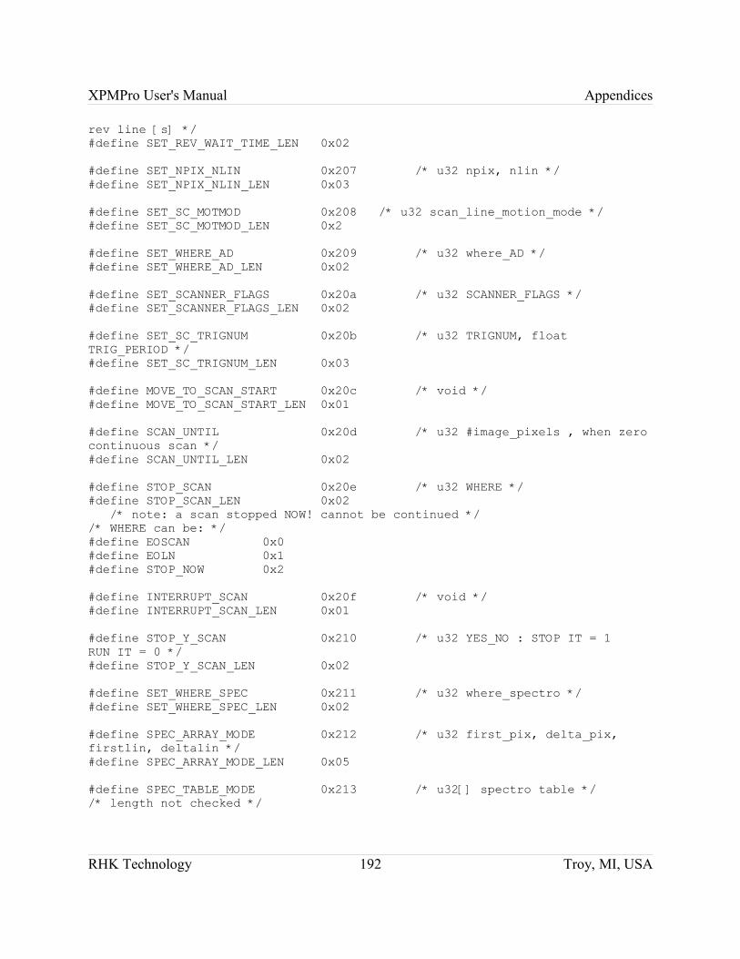
XPMPro User's Manual Appendices
rev line [s] */#define SET_REV_WAIT_TIME_LEN 0x02
#define SET_NPIX_NLIN 0x207 /* u32 npix, nlin */ #define SET_NPIX_NLIN_LEN 0x03
#define SET_SC_MOTMOD 0x208 /* u32 scan_line_motion_mode */#define SET_SC_MOTMOD_LEN 0x2
#define SET_WHERE_AD 0x209 /* u32 where_AD */#define SET_WHERE_AD_LEN 0x02
#define SET_SCANNER_FLAGS 0x20a /* u32 SCANNER_FLAGS */#define SET_SCANNER_FLAGS_LEN 0x02
#define SET_SC_TRIGNUM 0x20b /* u32 TRIGNUM, float TRIG_PERIOD */#define SET_SC_TRIGNUM_LEN 0x03
#define MOVE_TO_SCAN_START 0x20c /* void */ #define MOVE_TO_SCAN_START_LEN 0x01
#define SCAN_UNTIL 0x20d /* u32 #image_pixels , when zero continuous scan */#define SCAN_UNTIL_LEN 0x02
#define STOP_SCAN 0x20e /* u32 WHERE */ #define STOP_SCAN_LEN 0x02 /* note: a scan stopped NOW! cannot be continued *//* WHERE can be: */#define EOSCAN 0x0#define EOLN 0x1#define STOP_NOW 0x2
#define INTERRUPT_SCAN 0x20f /* void */#define INTERRUPT_SCAN_LEN 0x01
#define STOP_Y_SCAN 0x210 /* u32 YES_NO : STOP IT = 1 RUN IT = 0 */#define STOP_Y_SCAN_LEN 0x02
#define SET_WHERE_SPEC 0x211 /* u32 where_spectro */#define SET_WHERE_SPEC_LEN 0x02
#define SPEC_ARRAY_MODE 0x212 /* u32 first_pix, delta_pix, firstlin, deltalin */#define SPEC_ARRAY_MODE_LEN 0x05
#define SPEC_TABLE_MODE 0x213 /* u32[] spectro table *//* length not checked */
RHK Technology 192 Troy, MI, USA
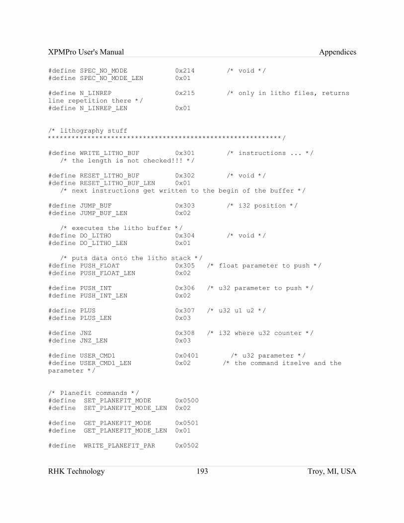
XPMPro User's Manual Appendices
#define SPEC_NO_MODE 0x214 /* void */#define SPEC_NO_MODE_LEN 0x01
#define N_LINREP 0x215 /* only in litho files, returns line repetition there */#define N_LINREP_LEN 0x01
/* lithography stuff ***********************************************************/
#define WRITE_LITHO_BUF 0x301 /* instructions ... */ /* the length is not checked!!! */
#define RESET_LITHO_BUF 0x302 /* void */#define RESET_LITHO_BUF_LEN 0x01 /* next instructions get written to the begin of the buffer */
#define JUMP_BUF 0x303 /* i32 position */#define JUMP_BUF_LEN 0x02
/* executes the litho buffer */#define DO_LITHO 0x304 /* void */#define DO_LITHO_LEN 0x01
/* puts data onto the litho stack */ #define PUSH_FLOAT 0x305 /* float parameter to push */#define PUSH_FLOAT_LEN 0x02
#define PUSH_INT 0x306 /* u32 parameter to push */#define PUSH_INT_LEN 0x02
#define PLUS 0x307 /* u32 u1 u2 */#define PLUS_LEN 0x03
#define JNZ 0x308 /* i32 where u32 counter */ #define JNZ_LEN 0x03
#define USER_CMD1 0x0401 /* u32 parameter */#define USER_CMD1_LEN 0x02 /* the command itselve and the parameter */
/* Planefit commands */#define SET_PLANEFIT_MODE 0x0500 #define SET_PLANEFIT_MODE_LEN 0x02
#define GET_PLANEFIT_MODE 0x0501#define GET_PLANEFIT_MODE_LEN 0x01
#define WRITE_PLANEFIT_PAR 0x0502
RHK Technology 193 Troy, MI, USA
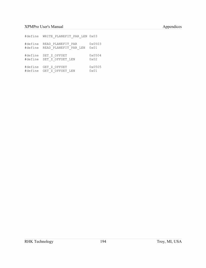
XPMPro User's Manual Appendices
#define WRITE_PLANEFIT_PAR_LEN 0x03
#define READ_PLANEFIT_PAR 0x0503#define READ_PLANEFIT_PAR_LEN 0x01
#define SET_Z_OFFSET 0x0504#define SET_Z_OFFSET_LEN 0x02
#define GET_Z_OFFSET 0x0505#define GET_Z_OFFSET_LEN 0x01
RHK Technology 194 Troy, MI, USA