Neoclassical Transport in QuasiAxially

Symmetric Stellarators

H.E.Mynick

Plasma Physics Laboratory, Princeton University

P.O. Box 451

Princeton, New Jersey 085430451, U.S.A.

Abstract

We present a numerical and analytic assessment of the transport in two

quasiaxially symmetric stellarators, including one variant of the MHH2

class[1] of such devices, and a conguration we refer to as NHH2, closely

related to MHH2. Monte Carlo simulation results are compared with ex-

pectations from established stellarator neoclassical theory, and with some

empirical stellarator scalings, used as an estimate of the turbulent transport

which might be expected. From the standpoint of transport, these may be

viewed as either tokamaks with large ( 1%) but lown ripple, or as stel-

larators with small ripple. For NHH2, numerical results are reasonably well

explained by analytic neoclassical theory. MHH2 adheres less to assump-

tions made in most analytic theory, and its numerical results agree less well

with theory than those for NHH2. However, for both, the nonaxisymmetric

contribution to the heat ux is comparable with the symmetric neoclassi-

cal contribution, and also falls into the range of the expected anomalous

1

(turbulent) contribution. Thus, it appears eort to further optimize the

thermal transport beyond the particular incarnations studied here would

be of at most modest utility. However, the favorable thermal connement

relies heavily on the radial electric eld. Thus, the present congurations

will have a loss cone for trapped energetic ions, so that further optimization

may be indicated for large devices of this type.

2

1. Introduction

This work describes an assessment of the connement characteristics of

two related stellarators having quasiaxial (QA) symmetry . We present

results for one variant of the MHH2 concept[1] | a 2period (N = 2) mod-

ular QA stellarator, and a second system we refer to as NHH2, obtained

from the MHH2 description, but modied in a simple manner (to be de-

scribed shortly) which makes it conform better to usual assumptions made

in existing stellarator transport theory, and therefore permits us to carry

the analytic development further. The principal objective of such magnetic

congurations is transport optimization, in this case by eliminating nonax-

isymmetric components of the magnetic eld strength B( ; ; ) in Boozer

coordinates, i.e., those harmonics with n 6= 0 in the decomposition

B( ; ; ) =Xm;n

Bmn( ) cos(n m): (1)

Then the residual neoclassical transport is as in a tokamak. If the ideal of

this conguration could be achieved, it would have the transport advantages

of the equivalent tokamak, while retaining the stellarator virtues of need-

ing no internal current to provide its rotational transform ( ) q1( ),

steadystate operation without current drive, and being more resistant to

disruptions.

The particular variant of MHH2 studied here is an Nc = 16 coil design,

with major radius R0 = 3m, average minor radius a = :66m, hence inverse

apsect ratio a a=R0 = 1=4:5, and average magnetic eld on axis B0 = 2

T. The shape of the outermost ux surface was specied by P. Garabedian,

and the magnetic elds computed[2] using the VMEC code.[3] Thus, the

ripple from the discreteness of the eld coils is neglected in this study, and is

3

expected not to produce appreciable transport except near the edge. NHH2

is a mathematical construct, having elds and other parameters precisely

the same as in MHH2, but with the sign of m reversed in each Bmn.

As desired, the average residual ripple strength in these systems is small

in comparison with that typical of stellarators, which have r=R0, but

is appreciable in comparison with that from coil disceteness in realistic toka-

maks. Since large ripple ( 1%) can also be problematic in tokamaks, it is

not a priori clear that the systems considered here will have acceptably low

neoclassical transport. Additionally, the nvalue associated with the ripple

here is about an order of magnitude lower than that normally envisioned

for rippled tokamaks. Thus, MHH2 and NHH2 have features which are not

strictly in accord with the assumptions made in existing transport theory for

both stellarators and tokamaks. One result of this work is to provide some

calibration of that theory with the MHH2 design. Especially important in

these theories is a separation in length scales between the toroidal connec-

tion length Lt qR0 and the length Lr Lt=jnq mj across a ripple well.The reversal of poloidal mode number m in the Bmn's makes this separation

better for NHH2. Thus one expects, and nds numerically, that transport

in NHH2 should adhere better with existing theory than that in MHH2.

The remainder of the paper is organized as follows. In Sec. 2 we de-

scribe the character of the elds and particle orbits in them, and brie y

review the theoretical transport results to which our numerical results will

be compared. In Sec. 3 we present the numerical results, transport coef-

cients obtained from Monte Carlo (MC) simulations done with GC3, a

guidingcenter (GC) code in Boozer coordinates, and compare these with

the analytical results already introduced. The ensembles used in the MC

4

runs are for monoenergetic particle distributions, in order to obtain adequate

statistics for ensembles of modest size. The approximate agreement between

the analytic and numerical results for NHH2 shown in Sec. 3 permits us in

Sec. 4 to perform a theorybased extension of the monoenergetic results to

the `energyaveraged' expressions applicable to a local Maxwellian distri-

bution fM , for the transport coecients, particle and energy uxes, and

associated connement times.

The ion uxes depend sensitively on the radial electric eld Er ' @r[with (r or ) the ambipolar potential and r (2 =B0)

1=2 a ux function

with units of length, representing the average minor radius], and these ana-

lytic expressions for the uxes put us in a position to determine those values

of Er which satisfy the ambipolarity constraint

0 =Xs

Zs1s; (2)

where s is a species label, Zs es=e0 is the charge number for species s,

e0 is the proton charge, and 1s is the particle ux for species s. Here, we

as usual consider a 2species plasma, electrons and a single ion species. As

found over a decade ago[4, 5], for some parameters multiple roots of Eq.(2)

can exist, of which two are stable to uctuations in Er. One, the `ion root,'

in which ions are held in by the electrons, is the one originally[6] and more

commonly considered. At the second, `electron root', the electrons are held

in by the ions, and the particle and heat uxes can be substantially reduced

from those in the ion root. Here we show that the version of NHH2 studied

here should be able to access this root. MHH2 is expected to display qualita-

tively similar behavior. Further reduction of nonaxisymmetric neoclassical

transport is useful only when it is larger than the rates of both symmetric

5

neoclassical and turbulent transport. Thus, in Sec. 5 we present some sum-

marizing discussion of the results of earlier sections, including a comparison

of the transport rates for these three mechanisms, with the turbulent rate

estimated from some common empirical stellarator connement scalings.

2. Fields, Orbits, and Existing Theory

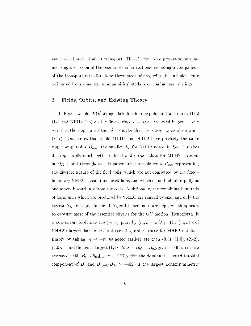
In Figs. 1 we plotB(x) along a eld line for one poloidal transit for MHH2

(1a) and NHH2 (1b) on the ux surface r = a=2. As noted in Sec. 1, one

sees that the ripple amplitude is smaller than the slower toroidal variation

( ). One notes that while MHH2 and NHH2 have precisely the same

ripple amplitudes Bmn, the smaller Lr for NHH2 noted in Sec. 1 makes

its ripple wells much better dened and deeper than for MHH2. Absent

in Fig. 1 and throughout this paper are those highern Bmn representing

the discrete nature of the eld coils, which are not computed by the xed

boundary VMEC calculations used here, and which should fall o rapidly as

one moves inward in r from the coils. Additionally, the remaining hundreds

of harmonics which are produced by VMEC are ranked by size, and only the

largest Nh are kept. In Fig. 1 Nh = 10 harmonics are kept, which appears

to capture most of the essential physics for the GC motion. Henceforth, it

is convenient to denote the (m;n)pairs by (m; ~n n=N). The (m; ~n) s of

NHH2's largest harmonics in descending order (those for MHH2 obtained

simply by taking m ! m as noted earlier) are then (0,0), (1,0), (2,-2),

(2,0),... and the tenth largest (1,1). Bm~n = B00 B0;0 gives the uxsurface

averaged eld, B1;0=B00jr=a ' :127 yields the dominant cos toroidalcomponent of B, and B2;2=B00 ' :028 is the largest nonaxisymmetric

6

contribution. The smallest Bm~n = B1;1 kept there is down by about 2

orders of magnitude from B0;0, and a factor of 4 from B2;2.

The general features of orbits in these elds are as envisioned in the

established literature on particle motion and neoclassical transport in stel-

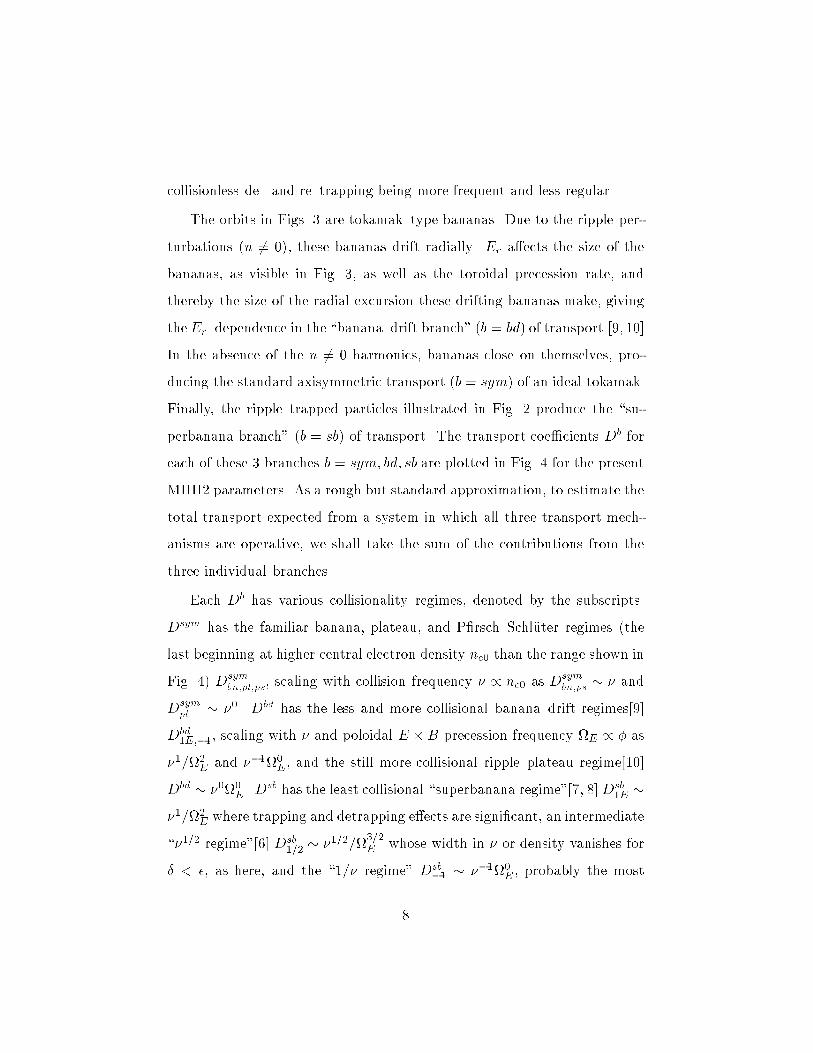
larators. In Figs. 2 and 3 we show poloidal projections of some collision-

less orbits representative of those dominantly contributing to neoclassical

transport in NHH2, for three values of the ambipolar eld, given by the

dimensionless variables R0eiEr=E or aeiEr=Ti (with E = 3:5

MeV the alpha birth energy, and Ti the ion temperature, which we take as

3.5 keV= E=103.): (a) = :01 ( = 2:2), (b) = 0 ( = 0), (c) = :01

( = 2:2). All are launched with kinetic energy K = 2T = 7 keV at

= 0 = and at small pitch vk=v. Those in Fig. 2 have = 0 and an

initial phase which makes them ripple trapped, while those in Fig. 3 have

= :2, which are toroidally trapped, like normal tokamak bananas.

For Er = 0, trapped particles [Fig. 2(b)] drift directly out of the ma-

chine. For nonzero Er, these `superbanana' orbits acquire a poloidal drift

which for 1 is large enough that the superbananas are well conned.

While particles initially ripple trapped sometimes remain trapped for the

entire poloidal transit [Fig. 2(c)], a more common situation is illustrated by

Fig. 2(a), where a particle initially ripple trapped can make successive colli-

sionless transitions from and back to that trapping state. Analytic theory of

this process[7, 8] assumes that sucient symmetry in B(x) exists that the

collisionless superbananas approximately close on themselves. This charac-

teristic is only roughly satised for NHH2, so that one might expect existing

theory to capture much of the transport physics here, though not all. Owing

to the larger Lr, collisionless orbits in MHH2 display less symmetry, with

7

collisionless de and retrapping being more frequent and less regular.

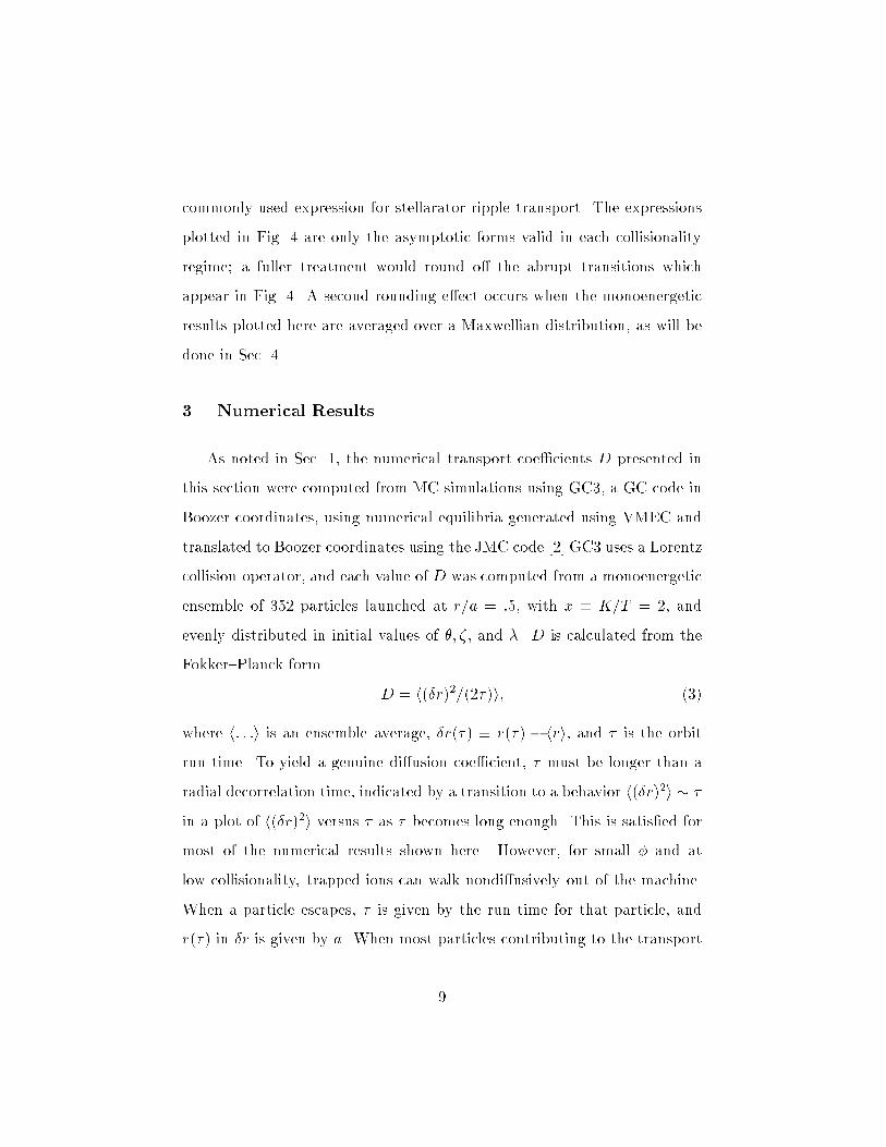
The orbits in Figs. 3 are tokamaktype bananas. Due to the ripple per-

turbations (n 6= 0), these bananas drift radially. Er aects the size of the

bananas, as visible in Fig. 3, as well as the toroidal precession rate, and

thereby the size of the radial excursion these drifting bananas make, giving

theErdependence in the \bananadrift branch" (b = bd) of transport.[9, 10]

In the absence of the n 6= 0 harmonics, bananas close on themselves, pro-

ducing the standard axisymmetric transport (b = sym) of an ideal tokamak.

Finally, the ripple trapped particles illustrated in Fig. 2 produce the \su-

perbanana branch" (b = sb) of transport. The transport coecients Db for

each of these 3 branches b = sym; bd; sb are plotted in Fig. 4 for the present

MHH2 parameters. As a rough but standard approximation, to estimate the

total transport expected from a system in which all three transport mech-

anisms are operative, we shall take the sum of the contributions from the

three individual branches.

Each Db has various collisionality regimes, denoted by the subscripts.

Dsym has the familiar banana, plateau, and PrschSchluter regimes (the

last beginning at higher central electron density ne0 than the range shown in

Fig. 4) Dsymbn;pl;ps, scaling with collision frequency / ne0 as D

symbn;ps and

Dsympl 0. Dbd has the less and more collisional bananadrift regimes[9]

Dbd1E;1, scaling with and poloidal E B precession frequency E / as

1=2E and 10

E, and the still more collisional rippleplateau regime[10]

Dbd 00

E . Dsb has the least collisional \superbanana regime"[7, 8]Dsb

1E 1=2

E where trapping and detrapping eects are signicant, an intermediate

\1=2 regime"[6] Dsb1=2 1=2=

3=2E whose width in or density vanishes for

< , as here, and the \1= regime" Dsb1 10

E , probably the most

8

commonly used expression for stellarator ripple transport. The expressions

plotted in Fig. 4 are only the asymptotic forms valid in each collisionality

regime; a fuller treatment would round o the abrupt transitions which

appear in Fig. 4. A second rounding eect occurs when the monoenergetic

results plotted here are averaged over a Maxwellian distribution, as will be

done in Sec. 4.

3. Numerical Results

As noted in Sec. 1, the numerical transport coecients D presented in

this section were computed from MC simulations using GC3, a GC code in

Boozer coordinates, using numerical equilibria generated using VMEC and

translated to Boozer coordinates using the JMC code.[2] GC3 uses a Lorentz

collision operator, and each value of D was computed from a monoenergetic

ensemble of 352 particles launched at r=a = :5, with x K=T = 2, and

evenly distributed in initial values of ; , and . D is calculated from the

FokkerPlanck form

D = h(r)2=(2)i; (3)

where h: : :i is an ensemble average, r() r() hri, and is the orbit

run time. To yield a genuine diusion coecient, must be longer than a

radial decorrelation time, indicated by a transition to a behavior h(r)2i

in a plot of h(r)2i versus as becomes long enough. This is satised for

most of the numerical results shown here. However, for small and at

low collisionality, trapped ions can walk nondiusively out of the machine.

When a particle escapes, is given by the run time for that particle, and

r() in r is given by a. When most particles contributing to the transport

9

have nondiusive motion, D in Eq.(3) no longer has a strict interpretation as

a diusion coecient, but still is an average reciprocal connement time[11]

(times a constant), and so is still a good measure of the connement quality

of the machine.

In Fig. 5 are shown numerical and analytic transport coecients for

NHH2 versus density ne0 (or ), for = 0. The 4 curves with symbols

are numerical results, and the 4 heavier curves without symbols are analytic

ones. The 3 lower analytic curves show each of the 3 transport branches, and

the top curve is their sum. The curve with diamond symbols shows MC re-

sults taking Nh = 2, i.e., taking only the two largest harmonics (0,0)+(1,0),

thus simulating the ideal tokamak nearest to the full MHH2 system. This

latter is approximated by the curve labeled Nh = 10 (star symbols). First

comparing the Nh = 2 curve with Dsym , one notes approximate agreement

between the numerical diusion and the axisymmetric neoclassical predic-

tion. Additionally, comparing theNh = 10 `full' results with the total (solid)

analytic curve, one again notes rough agreement. As ne0 ! 0, the analytic

curves become innite, with the onset of the 1= regime, while of course the

numerical results remain nite, and represent transport which is no longer

diusive. As already noted, the NHH2 elds do not fully satisfy assumptions

made in the original stellarator theories yielding the analytic expectations

plotted here, and thus the approximate agreement in Fig. 5 is as good as

one might expect.

Two other MC curves appear in Fig. 5, the results of two truncations of

the full elds to test the contribution to the transport of particular Bm~ns.

The curve labeled Nh = 3 (rectangular symbols) shows the transport from

keeping only the largest n 6= 0 harmonic (2,-2) in addition to the two

10

(0,0)+(1,0) kept for the Nh = 2truncation. One sees that the (2,-2) alone

accounts for about half the ripple transport of the full Nh = 10 system.

The curve labeled Nh = 4 (triangular symbols) gives the results of keeping

only the (0,1)+(0,-1) harmonics in addition to the (0,0)+(1,0) axisymmet-

ric ones. These yield a mirroring eld which can be problematic for some

stellarator congurations[12]. For the present case, however, one sees the

transport contribution from this mirroring perturbation is rather small.

Fig. 6 shows a sweep of MC results versus at ne0 = 3 1013=cm3, for

the full Nh = 10 and axisymmetric Nh = 2 cases. For simplicity, the value

for the ripplestrength required for the analytic curves is computed using

only the largest contributor B2;2. This makes the width of the analytic

peaks around or E = 0 broader for both Dbd and Dsb than one actually

expects as both mechanisms make the transition from their 1= to their

=2E behavior, and one sees the the Nh = 10 numerical results do indeed

have the peaked form of the analytic curves, but fall o somewhat faster

with .

In Fig. 7 we compare the simulation results for NHH2 already discussed

with those for MHH2. One notes that while being of comparable size, the

scaling of D with ne0 is somewhat dierent for MHH2, and is not as close to

the analytic prediction. Again, in general terms, this is expected, because

of the closer adherence in NHH2 of the spatial separation Lt=Lr 1. And

qualitatively, the lower transport levels for low ne0 is probably due to the

more prevalent collisionless detrapping enhancing the eective collision fre-

quency in this regime. However, a fuller understanding of the transport scal-

ing in MHH2 probably requires a theory dierent from the traditional ones

considered so far. Some work has been done[13] generalizing the banana

11

drift branch to perturbations which, like those here, have lown and m 6= 0.

Whether theory along these lines can clarify the MHH2 results in Fig. 7

is under study. For the present, however, both analytic and numerical in-

dications are that one may take the more complete results given here for

NHH2 as an estimate of the transport levels and scalings one may expect

for MHH2.

4. Energy Averaging and Ambipolar Potential

We have seen that existing analytic theory for stellarator transport pro-

vides an approximate understanding of the monoenergetic simulation results

for NHH2, though that conguration is somewhat dierent from the more

`classical' stellarators for which the theory was rst developed. On this ba-

sis, we analytically develop an expectation for the uxes one may expect

from a local Maxwellian distribution fM , and from these expressions, which

depend on the ambipolar electric eld Er, obtain a solution for the expected

ambipolar eld and predictions for the particle and heat uxes in the pres-

ence of that Er. The general procedure is like that used earlier[6, 4], but

includes the two transport branches b = sym; bd in addition to the sbbranch

considered in that earlier work.

For any function g(x K=T ) of the kinetic energy, the radial ux of g

for species s due to transport branch b is given by

bgs bgs=(ns0a) Zdvg(x)Db

s(x)@rfMs=(ns0a); (4)

where the normalized ux bgs is dened to have units of inverse time, so

that the connement time g for g is approximately given by 1=(4 g). Dbs(x)

12

is the monoenergetic diusion coecient examined in Sec. 3. Specializing g

to xr, for any power r, one may perform the velocity integration, nding[4]

xr =2

a2pf Db

s(r)[(an) + s 3

2(aT )] + Db

s(r+ 1)(aT )g; (5)

where n @r lnn0; T @r lnT , s aesEr=Ts, and

Db(r) PqDbq(x = 1)I(x; 1

2+mq+ r)j+ is Db(x) averaged over energy, and

hence over successive collisionality regimes q. The energy integral is given

by the incomplete Gamma function (n + 1; x) I(x; n) R x dx1xn1ex1 ,and the limits j+ denote those values x at which the collisionality regime

q of the transport mechanism changes. As mentioned in Sec. 2, the eect

of performing this integration is to smooth the abrupt transitions in the

transport coecients plotted in Fig. 4. From Eqs. 4 or 5, the normalized

particle ux is 1 (i.e., r = 0), and the heat ux is x (i.e., r = 1).

The symmetric contributions sym to the particle uxes are intrinsically

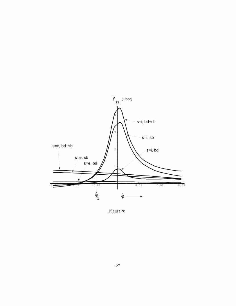
ambipolar, and thus do not play a role in determining Er. Thus, in Fig. 8

are plotted the nonaxisymmetric portions na = bd+ sb of versus , for

both ions and electrons, along with the constituent parts bd and sb. The

point 1 ' :01 at which na1i = na1e is a selfconsistent solution for Er at

the single radius r0 = a=2 for which this calculation has been carried out.

= 1 < 0 is the `ion root' more commonly considered. For the present

parameter choice, the second `electron root' 2 > 0 of the ambipolarity

constraint (2) does not occur, essentially because the ion ux or diusion

coecient does not fall o rapidly enough above = 0 to drop below the

slowly declining electron ux 1e before it falls below 0 due to e in Eq.(5).

Plotting the full energy uxes xs versus , and superposing the value

= 1 established from Fig. 8, in Fig. 9 one reads o the expected ion and

13

electron heat uxes for that case, and from this in Fig. 10 the predicted

neoclassical ion and electron energy connement times Es xs; (s = i; e);

nding Ei ' 44ms, and Ee ' 68ms.

The width of the peak in nai is proportional to collisionality. Thus, one

way of accessing the electron root for this system would be to operate at

lower density (or higher temperature). (A more precise criterion is given in

Ref. 4.) This is illustrated in Fig. 11, where the density is lowered by a factor

of 3, to ne0 = 1013. Now the electron root does appear, at 2 ' :03, while

the ion root is at 1 ' :004. One notes the property of 2 making it most

interesting: While at 1 the uxes are na1 ' 1:9=sec; naxi ' 12:0=sec, and

naxe ' 3:5=sec, at 2 these are substantially reduced: na1 ' :26=sec; naxi '1:6=sec, and naxe ' 1:6=sec.

5. Discussion

The NHH2 system employed in this work provides a bridge between

MHH2, which is the conguration of principal interest, for which adequate

analytic theory does not yet exist, and the more idealized existing analytic

theory. It is noteworthy that 2 systems having identical descriptions ex-

cept for the mapping m ! m which distinguishes them, can have rather

dierent transport scalings. However, we have also found that the overall

transport levels from the 2 systems are similar, so that our more detailed

understanding of NHH2's transport can be used to estimate that for MHH2.

Tailoring the harmonic content of the Bm~ns to further reduce na might

be worthwhile for MHH2 if na were large enough to dominate the sym-

metric neoclassical contribution sym as well as the anomalous (turbulent)

14

contribution an. To estimate the last of these, here we evaluate some com-

mon empirical stellarator scaling laws. However, it should be kept in mind

that, as recent tokamak experiments with transport barriers show, turbu-

lent transport is also a mechanism which may be amenable to substantial

reduction.

The nonaxisymmetric neoclassical contributions na to the uxes are

comparable to the symmetric ones, and for NHH2 na is dominated by

sb. At the ambipolarity solution = 1, for example, one nds symxi '

2:93; sbxi ' 2:23; bdxi ' 0:24. Most ions are in the rippleplateau regime of

bd, which has an nscaling Dbdrp n. Thus, since for the present system

n 4 is small compared with that (n 20) producing TF ripple in a normal

tokamak, bd is smaller by about a factor of 5 than its value for a normal

tokamak with comparable ripple, making the bananadrift contribution sub-

dominant.

Turning to the comparison of na with an, we evaluate the conne-

ment expected from the LacknerGottardi[14] and International Stellarator

Scaling[15] expressions. As in Ref. 15, the units here are MKS, except for

lineaveraged density n19, which is in units of 1019=m3 = 1013=cm3, heating

power PMW , which is in MW, and TeV , which is in eV.

LGE = 0:17Ra2n:619B:8q:4P:6MW (6)

ISS95E = :079R:65a2:21n:5119 B:83q:4P:59MW : (7)

Combining either of these with the power balance relation

E ' 22Ra2nT=P ' (:316 104)n19TeV =PMW (8)

15

yields a relation for E as a function of R; a; B; q, and n19. For n19 = 3, one

nds LGE ' 522msec, while ISS95E ' 21msec, with LGE independent of n19,

and ISS95E only weakly dependent on n19.

Thus, if ISS95E is assumed an accurate measure of turbulent transport,

that transport dominates the neoclassical transport computed earlier, and

further transport optimization from the congurations studied here would

be of no use. On the other hand, if LGE is taken as proper measure, then

the transport would be neoclassically dominated. However, since symxi

naxi , as noted above, even complete elimination of na would only result in

modest gains in the total Ei. Thus, further eort at optimization of thermal

transport from the conguration adopted here seems of limited utility.

While thermal transport is thus acceptably low in the present congu-

rations, it is strongly dependent on the radial eld Er for being so, with

xi reduced a factor of 8 from its = 0value at the operating point 1.

Thus, these systems will have a loss region for energetic ions. The existence

of this loss channel has sometimes been regarded as a virtue,[16] providing

a builtin means of alpha ash removal in return for a tolerable level of loss.

If the loss rate is judged excessive, however, little optimization has been

attempted on the conguration, and it seems likely that the loss could be

further reduced with additional eort at tailoring the magnetics.

Acknowledgment

This work supported by U.S.Department of Energy Contract No.DE-

AC02-76-CHO3073.

16

References

[1] P.R. Garabedian, Phys. Plasmas 3, 2483 (1996).

[2] L.P. Ku, A.H. Reiman, (private communications, 1996).

[3] S.P. Hirshman, J.C. Whitson, Phys. Fluids 26, 3553 (1986).

[4] H.E. Mynick, W.N.G. Hitchon, Nucl. Fusion 23, 1053 (1983).

[5] D.E. Hastings, W.A. Houlberg, K.C. Shaing, Nucl. Fusion 25 445

(1985).

[6] A.A. Galeev, R.Z. Sagdeev, H.P. Furth, M.N. Rosenbluth, Phys. Rev.

Letters 22, 511 (1969).

[7] A.A. Galeev,R.Z. Sagdeev, Sov. Phys. Usp. 12, 810 (1970).

[8] H.E. Mynick, Phys. Fluids 26, 2609-2615 (1983).

[9] R. Linsker, A.H. Boozer, Phys. Fluids 25, 143 (1982).

[10] A.H. Boozer, Phys. Fluids 23, 2283 (1983).

[11] H. Wobig, Z. Naturforsch. 37a, 906 (1982).

[12] J. Nuhrenberg (private communications, 1996).

[13] H.E. Mynick, Nucl. Fusion 26, 491 (1986).

[14] K. Lackner, N.A.O. Gottardi, NF 30, p767 (1990).

[15] U. Stroth, Murakami, R.A. Dory, H. Yamada, F. Sano, T. Obiki, Na-

tional Institute for Fusion Science Report NIFS-375 (1995).

[16] D.D.-M. Ho, R.M. Kulsrud, Phys. Fluids 30, 442 (1987).

17

Figures

Fig. 1. Plot of magnetic eld strength B(x) along B for one poloidal transit

at r = a=2 in (1a) MHH2, (1b)NHH2.

Fig. 2. Collisionless GC orbits launched with = 0; = 0 = , kinetic

energy K = 7 keV, and for 3 values of the ambipolar eld (a) = :01,(b) = 0, and (c) = :01.

Fig. 3. As Fig. 2, but with initial = 0:2.

Fig. 4. Analytic predictions for transport coecients Db for each of the

three operative transport branches b = sym; bd; sb, for jj = :002 and a

monoenergetic distribution with x K=T = 2, or x K=E = :002.

Fig. 5. Numerical (curves with symbols) and analytic (heavier curves with-

out symbols) transport results versus ne0 for = 0. See text for details.

Fig. 6. Transport results versus for ne0 = 3 1013=cm3. See text for

details.

Fig. 7. D versus ne0 for = 0, comparing transport in MHH2 with NHH2.

As in Fig. 5, the analytic theory is shown by curves without symbols.

Fig. 8. Plots of na1s = bd1s + sb1s and

bd1s and

sb1s versus , for s = e; i and at

ne0 = 3 1013.

The point 1 where na1i = na1e is a selfconsistent solution for the am-

bipolar eld Er.

Fig. 9. Plot of xs for s = i; e versus , for the same parameters as in Fig. 8.

18

Fig. 10. Plot of energy connement times Es for s = i; e, for the same

parameters as in Figs. 8 and 9.

Fig. 11. Plot of 1s for s = i; e versus , for the same parameters as in Fig. 8,

except at lower density (ne0 = 1013), in order to access the electron root

2, as well as the ion root 1 present in Fig. 8.

19

-1 -0.5 0.5 1

1.7

1.8

1.9

2.1

2.2

-1 -0.5 0.5 1

1.7

1.8

1.9

2.1

2.2

B(Tesla)

B(Tesla)

θ/π

θ/π

(a)

(b)

Figure 1:

20

225 250 275 300 325 350 375 -75

-50

-

25

0

25

50

7

5

R

z(a)

225 250 275 300 325 350 375 -75

-50

-

25

0

25

50

7

5z

R

(b)

225 250 275 300 325 350 375 -75

-50

-

25

0

25

50

7

5z

R

(c)

Figure 2:

21

225 250 275 300 325 350 375 -75

-50

-

25

0

25

50

7

5z

R

(a)

225 250 275 300 325 350 375 -75

-50

-

25

0

25

50

7

5z

R

(b)

225 250 275 300 325 350 375 -75

-50

-

25

0

25

50

7

5z

R

(c)

Figure 3:

22

0 132. 10

134. 10

136. 10

138. 10

141. 10

2500

5000

7500

10000

12500

15000

17500

20000

D(c

m /

sec)

2

ν≈Ω (δε)E

1/2

ν≈εΩ /(qn)E

ν≈ ε v (qn) nR

3/2

ν=ν ≡ε v/qR3/2∗

n (cm )e0

-3

D1E

bdbd

D-1

Dbd

rp

Dsym

bn

Dsym

pl

Dsb

1E

Dsb

-1

Figure 4:

23

0 132. 10

134. 10

136. 10

138. 10

141. 10

2500

5000

7500

10000

12500

15000

17500

20000

0

D(c

m /

sec)

2

n (cm )e0

-3

hN =10

N =3h

N =2hN =4

h

Dsym

Dsym+bd+sb

Dbd D

sb

Figure 5:

24

-0.02 -0.01 0 0.01 0.02

2500

5000

7500

10000

12500

15000

17500

20000D

(cm

/se

c)2

N =10h

N =2h

Dsym

Dbd

Dsb

Dsym+bd+sb

φ^

Figure 6:

25

2·10 13 4·10 13 6·10 13 8·10 13 1·10 14

2500

5000

7500

10000

12500

15000

17500

20000

MHH2

NHH2

Dsym+bd+sb

DsymD

bd Dsb

D(c

m /

sec)

2

Figure 7:

26

-0.03 -0.02 -0.01 0.01 0.02 0.03

1

2

3

4

γ1s

(1/sec)

φ

s=i, bd+sb

s=i, sb

s=i, bds=e, bd+sb

s=e, sbs=e, bd

φ1

Figure 8:

27

-0.03 -0.02 -0.01 0.01 0.02 0.03

5

10

15

20

25

φ

γxs

s=i

s=e

φ1

Figure 9:

28

-0.03 -0.02 -0.01 0.01 0.02 0.03

0.02

0.04

0.06

0.08

0.1

0.12

0.14

φ1

φ

τEs

s=e

s=i

Figure 10:

29

-0.03 -0.02 -0.01 0.01 0.02 0.03

2

4

6

8

10

12

φφ1 φ

2

γ1s

s=i

s=e

Figure 11:

30