Yadav Pandit, Ph.D., July 2012 NUCLEAR PHYSICS ... Pandit July 2012 Dissertation written by Yadav Pandit B. Sc., Tribhuvan University, Nepal, 1993 M. Sc., Tribhuvan University, Nepal,

Yadav Pandit, Ph.D., July 2012 NUCLEAR PHYSICS

AZIMUTHAL ANISOTROPY IN HEAVY ION COLLISIONS (169 pp.)

Director of Dissertation : Prof. Declan Keane

STAR (Solenoidal Tracker At RHIC) is one of two large detectors along the ring of the

Relativistic Heavy Ion Collider (RHIC) at Brookhaven National Laboratory. Experiments

that collide heavy nuclei at high energy have been taking data at RHIC since the year 2000.

The main goal of RHIC has been to search for a new phase of matter called the Quark Gluon

Plasma (QGP), and to determine its properties, including the phase diagram that governs

the relationship between QGP and more conventional hadronic matter. This dissertation has

a particular focus on analysis of STAR measurements of the anisotropy of particle emission

over a range of colliding energies, and these particular measurements are made possible by

a unique application of a detector subsystem called Beam-Beam Counters (BBCs), which

are placed close to the beam lines on both sides of the collision region. This project has

involved development of software that uses the hit pattern of charged particles in the BBCs

to determine the collision reaction plane, for use in measurements of anisotropy.

Anisotropic flow sheds light on the early partonic system, and according to models,

is minimally distorted during the post-partonic stages of the collision. In this anisotropic

flow analysis, the estimated reaction plane of each event is reconstructed using the BBC

signals, which have a large rapidity gap between them. There is also a large rapidity gap

between each BBC and the STAR Time Projection Chamber (the main STAR subsystem

for measuring particle tracks). These large rapidity gaps allow us to measure correlations

relative to the reaction plane with the least possible systematic error from what is known as

“non-flow”, i.e., background correlations unrelated to the reaction plane.

Flow correlations are normally reported in terms Fourier coefficients, v1, v2, etc. Di-

rected flow is quantified by the first harmonic (v1) in the Fourier expansion of the particle’s

azimuthal distribution with respect to the reaction plane. Elliptic flow is the name given

to the second harmonic (v2), and triangular flow is the name for the third harmonic (v3).

These harmonic coefficients carry information on the very early stages of the collision.

The v1 component is emphasized in this dissertation, and the BBC information that is a

unique feature of this work is especially important for v1 measurements. Until recently,

higher-order odd harmonics were overlooked. These odd flow harmonics carry valuable

information about the initial-state fluctuations of the colliding system. This dissertation

includes a study of the flow harmonic related to dipole asymmetry and triangularity in the

initial geometry.

AZIMUTHAL ANISOTROPY IN HEAVY ION COLLISIONS

A dissertation submitted to

Kent State University in partial

fulfillment of the requirements for the

degree of Doctor of Philosophy

by

Yadav Pandit

July 2012

Dissertation written by

Yadav Pandit

B. Sc., Tribhuvan University, Nepal, 1993

M. Sc., Tribhuvan University, Nepal, 1996

Ph.D., Kent State University, 2012

Approved by

Dr. Declan Keane, Professor, Physics

Chair, Doctoral Dissertation Committee

Dr. Spyridon Margetis, Professor, Physics

Dr. Bryon Anderson, Professor, Physics

Dr. Antal I. Jakli, Professor, Liquid Crystal Institute

Dr. Mark L. Lewis, Professor, Mathematics

Accepted by

Dr. James T. Gleeson, Chair, Department of Physics

Dr. Raymond A. Craig, Dean, College of Arts

and Sciences

ii

Table of Contents

List of Figures . . . . . . . . . . . . . . . . . . . . . . . . . . . . . . . . . . . . . . viii

List of Tables . . . . . . . . . . . . . . . . . . . . . . . . . . . . . . . . . . . . . . xx

Acknowledgements . . . . . . . . . . . . . . . . . . . . . . . . . . . . . . . . . . . xxi

1 INTRODUCTION . . . . . . . . . . . . . . . . . . . . . . . . . . . . . . . . . 1

1.1 Heavy Ion Collisions . . . . . . . . . . . . . . . . . . . . . . . . . . . . . 1

1.2 Quark Gluon Plasma and the QCD Phase Diagram . . . . . . . . . . . . . 3

1.3 Beam Energy Scan at RHIC . . . . . . . . . . . . . . . . . . . . . . . . . 4

1.4 Physics Observables for RHIC Energy Scan . . . . . . . . . . . . . . . . . 6

1.4.1 QGP Signatures . . . . . . . . . . . . . . . . . . . . . . . . . . . . 6

1.4.2 Signatures of a Phase Transition and a Critical Point . . . . . . . . 12

1.5 Outline of Current Work . . . . . . . . . . . . . . . . . . . . . . . . . . . 16

2 ANISOTROPIC FLOW . . . . . . . . . . . . . . . . . . . . . . . . . . . . . . 19

2.1 Introduction . . . . . . . . . . . . . . . . . . . . . . . . . . . . . . . . . . 19

2.2 Flow Components . . . . . . . . . . . . . . . . . . . . . . . . . . . . . . . 21

2.2.1 Directed Flow . . . . . . . . . . . . . . . . . . . . . . . . . . . . . 21

2.2.2 Elliptic Flow . . . . . . . . . . . . . . . . . . . . . . . . . . . . . 24

2.2.3 Dipole Asymmetry and Triangular Flow . . . . . . . . . . . . . . . 26

2.3 Flow Fluctuations . . . . . . . . . . . . . . . . . . . . . . . . . . . . . . . 28

2.4 Non Flow Correlations . . . . . . . . . . . . . . . . . . . . . . . . . . . . 29

iii

2.5 Model Calculations . . . . . . . . . . . . . . . . . . . . . . . . . . . . . . 30

2.5.1 RQMD . . . . . . . . . . . . . . . . . . . . . . . . . . . . . . . . 30

2.5.2 UrQMD . . . . . . . . . . . . . . . . . . . . . . . . . . . . . . . . 32

2.5.3 AMPT . . . . . . . . . . . . . . . . . . . . . . . . . . . . . . . . 32

3 EXPERIMENTAL DETAILS . . . . . . . . . . . . . . . . . . . . . . . . . . 34

3.1 The Relativistic Heavy Ion Collider . . . . . . . . . . . . . . . . . . . . . 34

3.2 The STAR Detector . . . . . . . . . . . . . . . . . . . . . . . . . . . . . . 36

3.2.1 The Time Projection Chamber . . . . . . . . . . . . . . . . . . . . 39

3.2.2 Forward Time Projection Chamber . . . . . . . . . . . . . . . . . . 43

3.2.3 Beam Beam Counters . . . . . . . . . . . . . . . . . . . . . . . . 43

3.2.4 Time of Flight . . . . . . . . . . . . . . . . . . . . . . . . . . . . 45

3.2.5 VPD . . . . . . . . . . . . . . . . . . . . . . . . . . . . . . . . . 47

3.2.6 ZDC . . . . . . . . . . . . . . . . . . . . . . . . . . . . . . . . . 49

3.2.7 The STAR Trigger . . . . . . . . . . . . . . . . . . . . . . . . . . 50

4 ANALYSIS DETAILS . . . . . . . . . . . . . . . . . . . . . . . . . . . . . . . 51

4.1 Data Sets . . . . . . . . . . . . . . . . . . . . . . . . . . . . . . . . . . . 51

4.1.1 Event Selection . . . . . . . . . . . . . . . . . . . . . . . . . . . . 52

4.1.2 Centrality Determination . . . . . . . . . . . . . . . . . . . . . . . 53

4.1.3 Track Selections . . . . . . . . . . . . . . . . . . . . . . . . . . . 56

4.1.4 Particle Identification . . . . . . . . . . . . . . . . . . . . . . . . . 56

4.2 Flow Analysis Methods . . . . . . . . . . . . . . . . . . . . . . . . . . . . 58

4.2.1 Event Plane method . . . . . . . . . . . . . . . . . . . . . . . . . 58

4.2.2 Estimation of Event Plane from TPC/FTPC . . . . . . . . . . . . . 59

iv

4.2.3 Event Plane with BBC . . . . . . . . . . . . . . . . . . . . . . . . 60

4.2.4 Simulation Study of BBC Event Plane . . . . . . . . . . . . . . . . 60

4.2.5 BBC Event Plane from Real Data Production . . . . . . . . . . . . 61

4.2.6 Event Plane Distribution . . . . . . . . . . . . . . . . . . . . . . . 63

4.2.7 Event Plane Resolution . . . . . . . . . . . . . . . . . . . . . . . . 72

4.3 Directed Flow Measurement . . . . . . . . . . . . . . . . . . . . . . . . . 75

4.3.1 BBC Event Plane Method . . . . . . . . . . . . . . . . . . . . . . 75

4.3.2 FTPC Event Plane Method . . . . . . . . . . . . . . . . . . . . . 76

4.4 Elliptic Flow Measurement . . . . . . . . . . . . . . . . . . . . . . . . . . 77

4.4.1 BBC Event Plane Method . . . . . . . . . . . . . . . . . . . . . . 77

4.4.2 TPC Event Plane Method . . . . . . . . . . . . . . . . . . . . . . . 77

4.4.3 The Cumulant Method . . . . . . . . . . . . . . . . . . . . . . . . 78

4.5 Triangular Flow Measurement . . . . . . . . . . . . . . . . . . . . . . . . 79

4.5.1 Event Plane Methods . . . . . . . . . . . . . . . . . . . . . . . . . 80

4.5.2 Two-Particle Correlation Method . . . . . . . . . . . . . . . . . . 80

4.6 Flow Harmonic Associated with Dipole Asymmetry . . . . . . . . . . . . 82

4.6.1 Scalar Product Method . . . . . . . . . . . . . . . . . . . . . . . . 83

4.6.2 Event Plane method . . . . . . . . . . . . . . . . . . . . . . . . . 84

4.7 Systematic Uncertainties . . . . . . . . . . . . . . . . . . . . . . . . . . . 84

4.7.1 Event Plane Determination . . . . . . . . . . . . . . . . . . . . . . 85

4.7.2 Detector Acceptance and Efficiency . . . . . . . . . . . . . . . . . 85

4.7.3 East-West Symmetry . . . . . . . . . . . . . . . . . . . . . . . . . 85

4.7.4 Non-Flow Effect . . . . . . . . . . . . . . . . . . . . . . . . . . . 86

5 RESULTS – I: DIRECTED FLOW . . . . . . . . . . . . . . . . . . . . . . . . 87

v

5.1 Directed Flow in 7.7, 11.5, 19.6, 27 and 39 GeV AuAu Collisions . . . . . 87

5.1.1 Charged Particles . . . . . . . . . . . . . . . . . . . . . . . . . . 87

5.1.2 Identified Charged Particles . . . . . . . . . . . . . . . . . . . . . 94

5.2 Directed Flow in 22.4 GeV CuCu Collisions . . . . . . . . . . . . . . . . 104

5.3 Directed Flow in 9.2 GeV AuAu Collisions . . . . . . . . . . . . . . . . . 106


5.5 Summary . . . . . . . . . . . . . . . . . . . . . . . . . . . . . . . . . . . 109

6 RESULTS – II: ELLIPTIC FLOW . . . . . . . . . . . . . . . . . . . . . . . . 112

6.1 AuAu Collisions at 7.7, 11.5, 19.6, 27 and 39 GeV . . . . . . . . . . . . . 112

6.1.1 Pseudorapidity and Transverse Momentum Dependence . . . . . . 112

6.1.2 Method Comparison . . . . . . . . . . . . . . . . . . . . . . . . . 114

6.1.3 Beam Energy Dependence . . . . . . . . . . . . . . . . . . . . . . 116

6.2 CuCu Collisions at 22.4 GeV . . . . . . . . . . . . . . . . . . . . . . . . . 117


6.4 Summary . . . . . . . . . . . . . . . . . . . . . . . . . . . . . . . . . . . 122

7 RESULTS – III: TRIANGULAR FLOW . . . . . . . . . . . . . . . . . . . . . 124

7.1 Centrality dependence . . . . . . . . . . . . . . . . . . . . . . . . . . . . 124

7.2 ∆η dependence . . . . . . . . . . . . . . . . . . . . . . . . . . . . . . . . 126

7.3 η and pT dependence . . . . . . . . . . . . . . . . . . . . . . . . . . . . . 128

7.4 Comparisons with other experiments . . . . . . . . . . . . . . . . . . . . . 128

7.5 Model Comparisons . . . . . . . . . . . . . . . . . . . . . . . . . . . . . . 132

7.6 Systematic Uncertanities . . . . . . . . . . . . . . . . . . . . . . . . . . . 133

7.7 Summary . . . . . . . . . . . . . . . . . . . . . . . . . . . . . . . . . . . 134

vi

8 RESULTS – IV: DIPOLE ASYMMETRY . . . . . . . . . . . . . . . . . . . . 135

8.1 Pseudorapidity Dependence . . . . . . . . . . . . . . . . . . . . . . . . . . 135

8.2 Transverse Momentum Dependence . . . . . . . . . . . . . . . . . . . . . 137

8.3 Centrality Dependence . . . . . . . . . . . . . . . . . . . . . . . . . . . . 138

8.4 Model Comparisons . . . . . . . . . . . . . . . . . . . . . . . . . . . . . . 139


8.6 Summary . . . . . . . . . . . . . . . . . . . . . . . . . . . . . . . . . . . 140

9 SUMMARY AND CONCLUSIONS . . . . . . . . . . . . . . . . . . . . . . . 142

Bibliography . . . . . . . . . . . . . . . . . . . . . . . . . . . . . . . . . . . . . . 148

A AUTHOR’S CONTRIBUTION TO COLLABORATIVE RESEARCH . . . . 154

B PRESENTATIONS AND PUBLICATION . . . . . . . . . . . . . . . . . . . . 157

vii

List of Figures

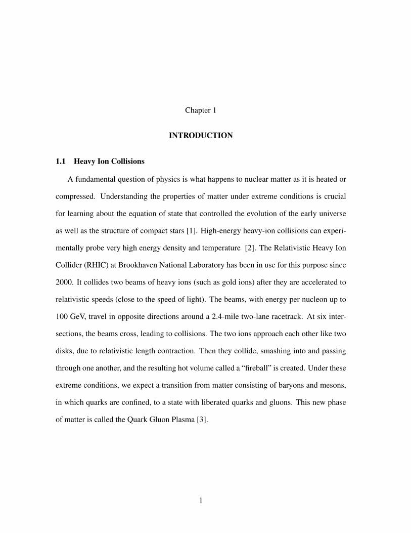
1.1 Collision of two nuclei A and B, with a non-zero impact parameter. The

participants and the spectators are also shown. The nuclei have a spheri-

cal shape in their own rest frames, but are Lorentz-contracted when accel-

erated. At maximum RHIC energy, the contraction factor (about 100) is

much greater than illustrated here. . . . . . . . . . . . . . . . . . . . . . . 2

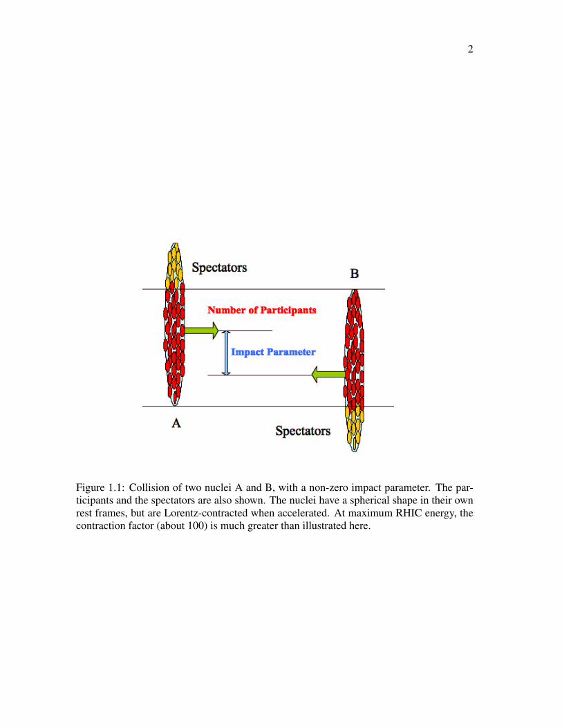
1.2 Space-time diagram and different evolution stages of a relativistic heavy-

ion collision . . . . . . . . . . . . . . . . . . . . . . . . . . . . . . . . . . 3

1.3 Schematic picture of QCD phase diagram shown in T − µB space . . . . . 5

1.4 Identified particle v2 as a function of mT − m scaled by number of con-

stituent quarks at 200 GeV [15]. . . . . . . . . . . . . . . . . . . . . . . . 7

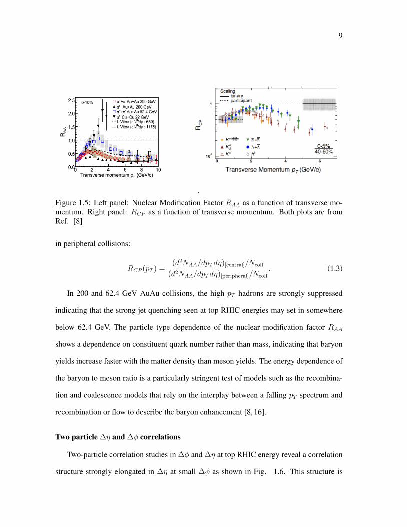
1.5 Left panel: Nuclear Modification Factor RAA as a function of transverse

momentum. Right panel: RCP as a function of transverse momentum.

Both plots are from Ref. [8] . . . . . . . . . . . . . . . . . . . . . . . . . 9

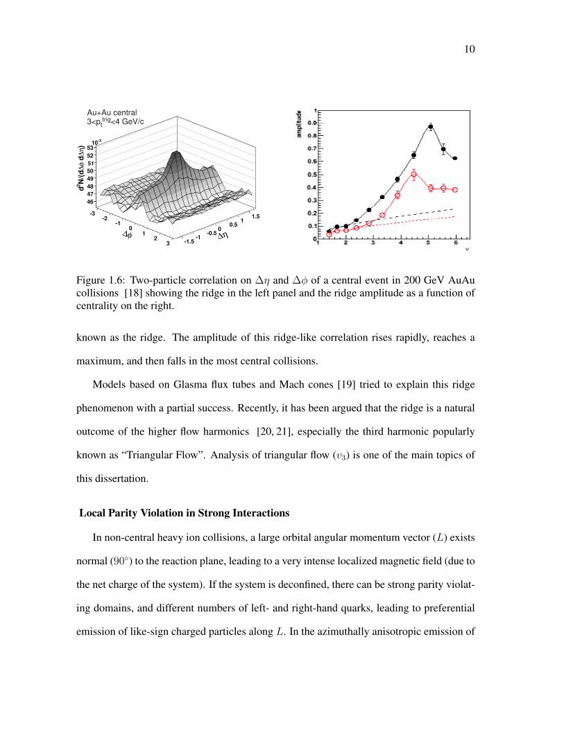
1.6 Two-particle correlation on ∆η and ∆φ of a central event in 200 GeV

AuAu collisions [18] showing the ridge in the left panel and the ridge

amplitude as a function of centrality on the right. . . . . . . . . . . . . . . 10

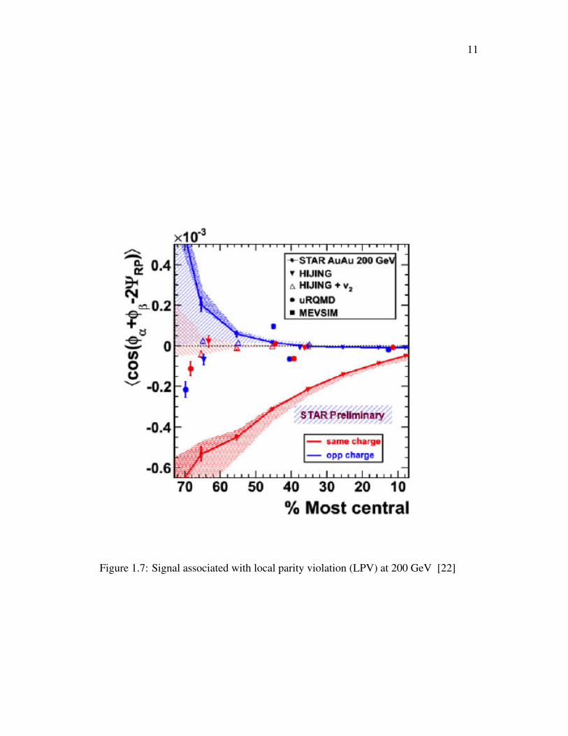
1.7 Signal associated with local parity violation (LPV) at 200 GeV [22] . . . . 11

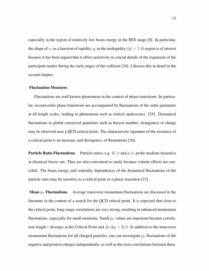
1.8 Event-wise mean pT distribution for the most central AuAu collisions at

200 GeV, measured in the STAR experiment [28] . . . . . . . . . . . . . . 14

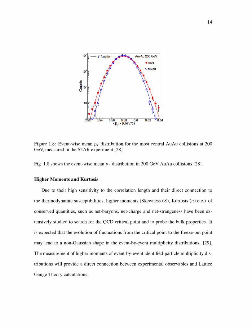
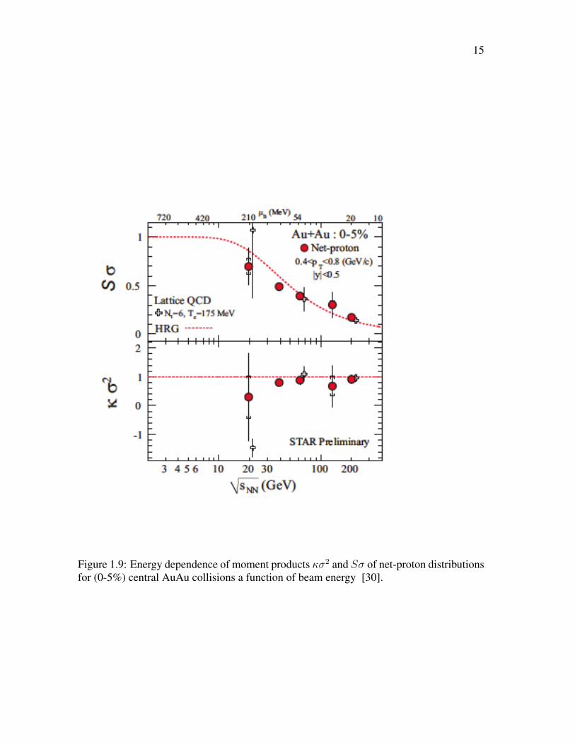
1.9 Energy dependence of moment products κσ2 and Sσ of net-proton distri-

butions for (0-5%) central AuAu collisions a function of beam energy [30]. 15

viii

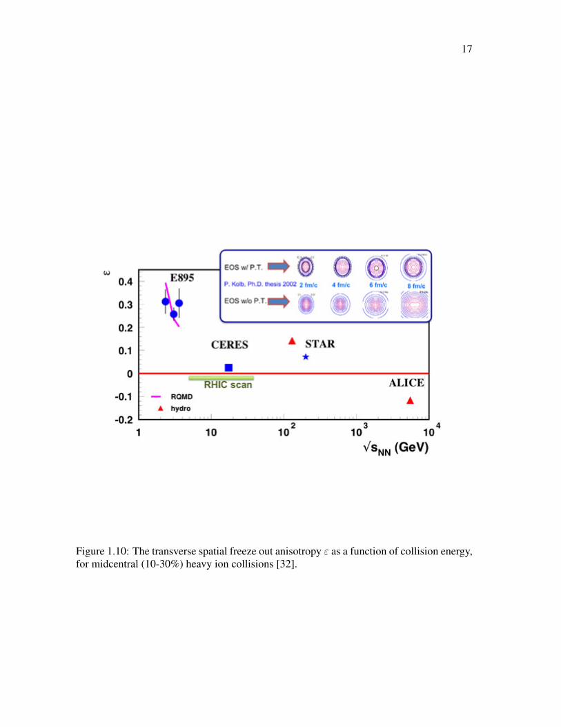
1.10 The transverse spatial freeze out anisotropy ε as a function of collision

energy, for midcentral (10-30%) heavy ion collisions [32]. . . . . . . . . . 17

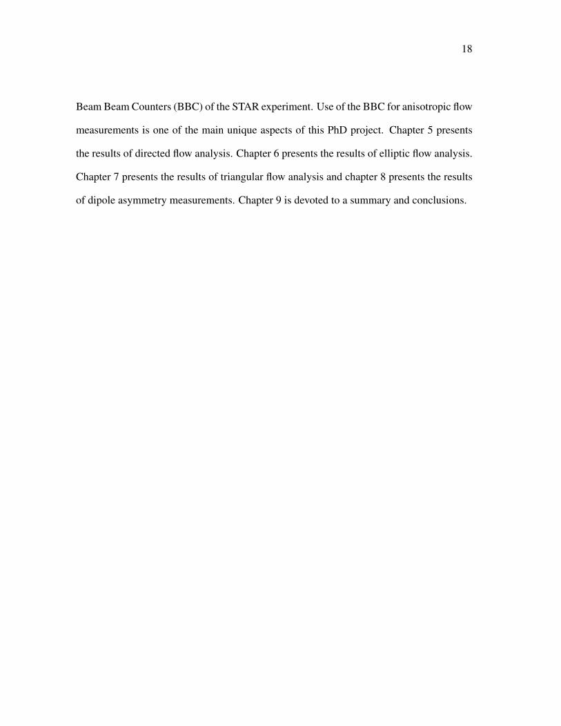
2.1 Event anisotropy in spatial and momentum space with respect to the reac-

tion plane. . . . . . . . . . . . . . . . . . . . . . . . . . . . . . . . . . . . 19

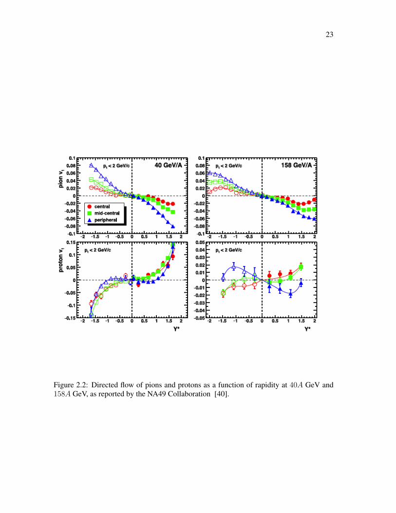
2.2 Directed flow of pions and protons as a function of rapidity at 40A GeV

and 158A GeV, as reported by the NA49 Collaboration [40]. . . . . . . . . 23

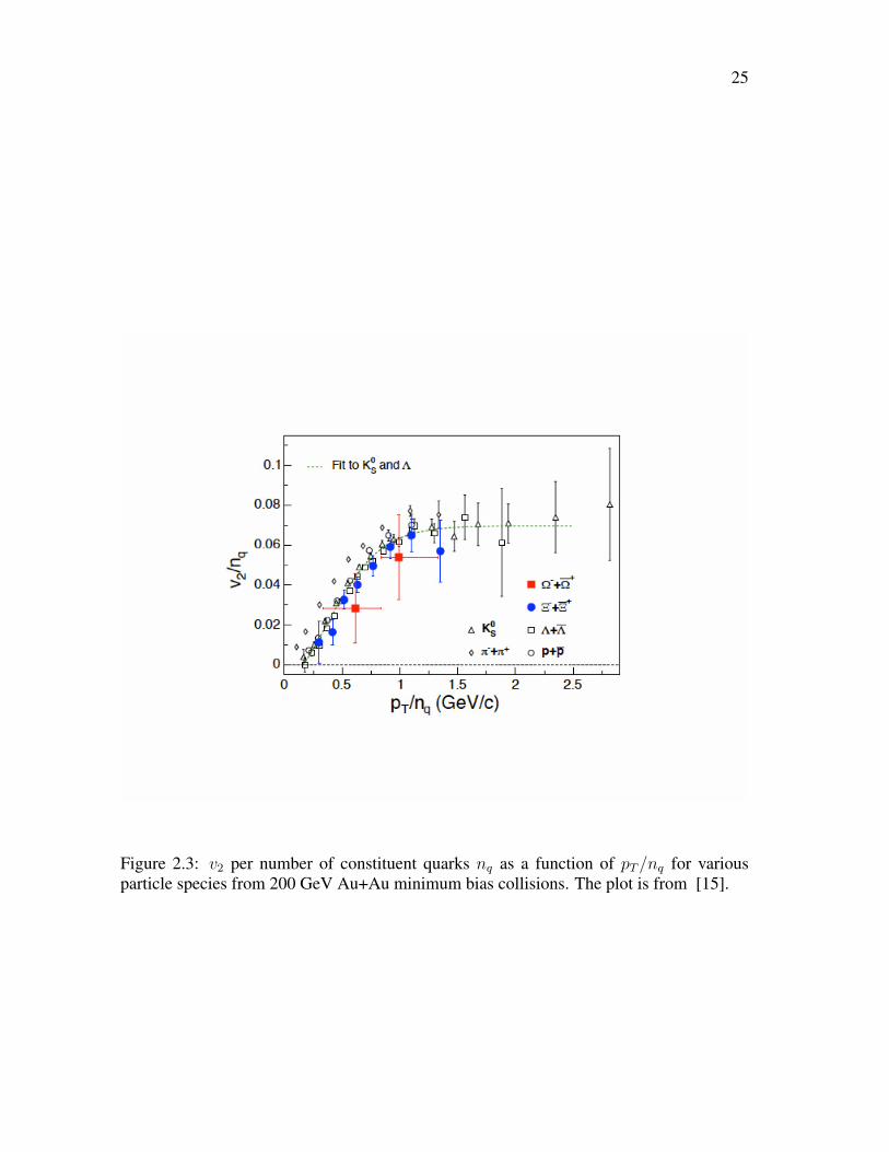
2.3 v2 per number of constituent quarks nq as a function of pT/nq for various

particle species from 200 GeV Au+Au minimum bias collisions. The plot

is from [15]. . . . . . . . . . . . . . . . . . . . . . . . . . . . . . . . . . 25

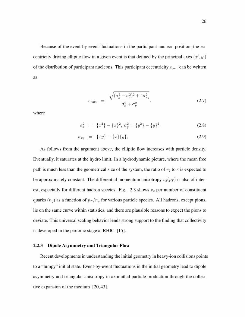
2.4 Energy density distribution in the transverse plane for one event, show-

ing triangular anisotropy in the initial geometry. This plot is taken from

Ref. [45]. . . . . . . . . . . . . . . . . . . . . . . . . . . . . . . . . . . . 27

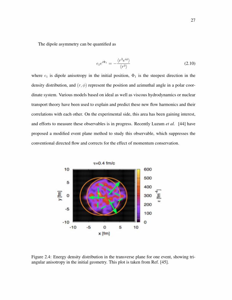
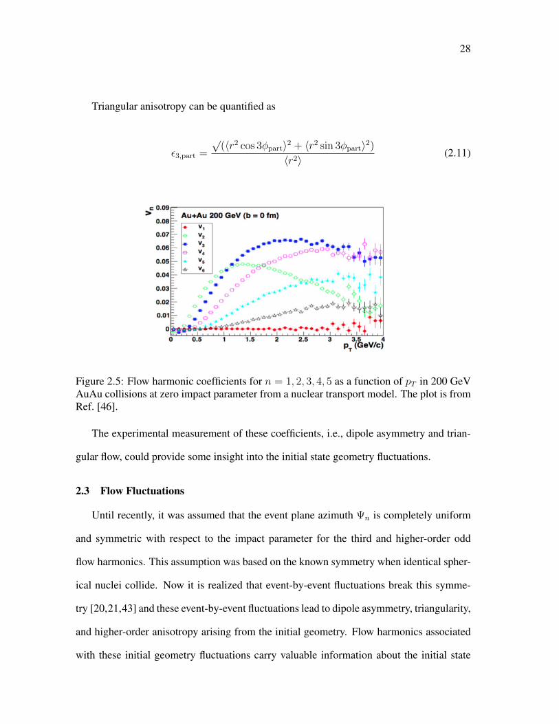
2.5 Flow harmonic coefficients for n = 1, 2, 3, 4, 5 as a function of pT in 200

GeV AuAu collisions at zero impact parameter from a nuclear transport

model. The plot is from Ref. [46]. . . . . . . . . . . . . . . . . . . . . . . 28

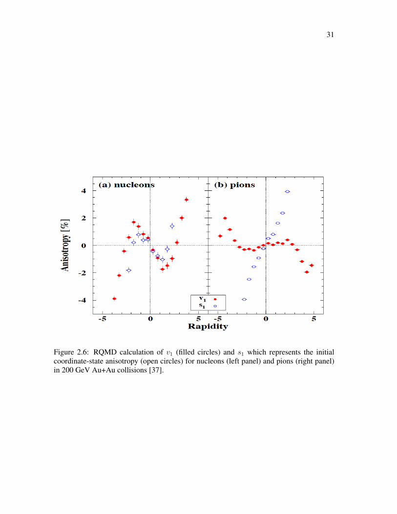
2.6 RQMD calculation of v1 (filled circles) and s1 which represents the ini-

tial coordinate-state anisotropy (open circles) for nucleons (left panel) and

pions (right panel) in 200 GeV Au+Au collisions [37]. . . . . . . . . . . . 31

3.1 Aerial view of the Relativistic Heavy Ion Collider (RHIC) complex at

Brookhaven National Laboratory. . . . . . . . . . . . . . . . . . . . . . . . 34

3.2 A diagram of the Relativistic Heavy Ion Collider (RHIC) complex at Brookhaven

National Laboratory. The complex is composed of long chain of particle

accelerators. . . . . . . . . . . . . . . . . . . . . . . . . . . . . . . . . . . 35

ix

3.3 The STAR detector systems showing the location of the detector subsystems. 37

3.4 Cross-section of the STAR detectors used in year 2010 showing the loca-

tion of the detector sub-systems. . . . . . . . . . . . . . . . . . . . . . . . 38

3.5 Beam’s eye (left) and side (right) views of a central AuAu collision at 200

GeV. . . . . . . . . . . . . . . . . . . . . . . . . . . . . . . . . . . . . . . 39

3.6 The STAR TPC is centered on the 6 o’clock intersection region at RHIC.

This figure is taken from Ref. [55]. . . . . . . . . . . . . . . . . . . . . . . 40

3.7 The energy loss (dE/dx) distribution for various particles as measured by

the TPC as a function of total momentum (p) of the particles. . . . . . . . . 42

3.8 Forward Time Projection Chamber. . . . . . . . . . . . . . . . . . . . . . . 44

3.9 A diagram of the STAR Beam Beam Counters: a similar array is located

on both the east and west sides of the STAR detector. . . . . . . . . . . . . 45

3.10 Two side views of a Multigap Resistive Plate Chamber (MRPC) module.

The figure is taken from Ref. [60]. . . . . . . . . . . . . . . . . . . . . . . 46

3.11 Pseudo-vertex position detector (pVPD), with one located on each side of

the STAR detector . . . . . . . . . . . . . . . . . . . . . . . . . . . . . . 48

3.12 Particle identification using the STAR Time of Flight (TOF) detector. Pro-

ton, kaon, pion and electron bands are clearly separated. . . . . . . . . . . 49

4.1 Uncorrected dN/dη measured within |η| < 0.5 in the TPC from√sNN =

7.7 to 39 GeV in AuAu collisions shown as black points. The red curves

show the multiplicity distributions at√sNN = 7.7 to 39 GeV from Monte

Carlo Glauber simulations. . . . . . . . . . . . . . . . . . . . . . . . . . . 54

4.2 Mass squared versus magnetic rigidity (momentum per charge) for AuAu

collisions at√sNN =7.7 GeV. . . . . . . . . . . . . . . . . . . . . . . . . 57

x

4.3 BBC first order event plane resolution for RQMD events. This plot is from

Ref. [8]. . . . . . . . . . . . . . . . . . . . . . . . . . . . . . . . . . . . . 62

4.4 East ADC distribution for the first inner ring of BBC. These are online

monitoring plots from 39 GeV AuAu collisions during data taking in 2010

and no trigger selection was made. . . . . . . . . . . . . . . . . . . . . . . 64

4.5 West ADC distribution for the first inner ring of BBC. These are online



4.6 East ADC distribution for the second inner ring of BBC. These are online



4.7 West ADC distribution for the second inner ring of BBC. These are online


and no trigger selection was made . . . . . . . . . . . . . . . . . . . . . . 67

4.8 Mean channel-by-channel east and west ADC distributions before and after

gain correction. This plot is from 22.4 GeV CuCu collisions for 20-30%

central collisions. . . . . . . . . . . . . . . . . . . . . . . . . . . . . . . . 68

4.9 First-order event plane distribution for east, west and full event plane. The

Ψ weight method is applied to force the event plane distribution to become

flat, as represented by the horizontal red line. . . . . . . . . . . . . . . . . 70

4.10 First-order event plane distribution for east, west and full event plane. The

shift correction forces the event plane distribution to became flat. . . . . . . 72

xi

4.11 The event plane resolution for the nth (n = km) harmonic of a particle

distribution with respect to the mth harmonic plane, as a function of χm =

vm/σ. This plot is from Ref. [14]. . . . . . . . . . . . . . . . . . . . . . . 73

4.12 The left panel shows the first-order BBC resolution from the sub-event cor-

relation between east and west BBCs. The right panel shows the resolution

correction for elliptic flow measurement using the first-order BBC event

plane. The BBC EP resolution is plotted as a function of centrality and for

different beam energies. . . . . . . . . . . . . . . . . . . . . . . . . . . . . 75

4.13 v23{2,∆η} vs. ∆η for charged hadrons within two centrality intervals in

200 GeV Au+Au collisions. Data are fit with narrow and wide Gaussians.

Like Sign, Unlike Sign, and Charge Independent cases are shown. . . . . . 81

5.1 Charged hadron v1 in AuAu collisions at 7.7 and 11.5 GeV as a function of

η for central (0−10%), mid-central (10−40%) and peripheral (40−80%)

collisions on the left. The panels on the right show the same measurement

but for a minimum-bias trigger selection (0− 80% centrality), along with a

transport model calculations. . . . . . . . . . . . . . . . . . . . . . . . . . 88

5.2 Charged hadron v1 in AuAu collisions at 19.6 and 27 GeV as a function of

η for central (0−10%), mid-central (10−40%) and peripheral (40−80%)




xii

5.3 Charged hadron v1 in AuAu collisions at 39 GeV as a function of η for

central (0 − 10%), mid-central (10 − 40%) and peripheral (40 − 80%)




5.4 Charged hadron v1 at mid rapidity as a function of η in the top panel for

central (0 − 10%), mid-central (10 − 40%) and peripheral (40 − 80%)

collisions for Au+Au at√sNN = 7.7, 11.5, 19.6, 27 and 39 GeV. The pT

range for this study is 0.2 < pT < 2.0 GeV/c. In the bottom panel, we show

charged hadron v1 as a function of pT for central (0 − 10%), mid-central

(10 − 40%) and peripheral (40 − 80%) collisions for Au+Au at√sNN =

7.7, 11.5, 19.6, 27 and 39 GeV. The pseudorapidity range for this study is

|η| < 1.0. . . . . . . . . . . . . . . . . . . . . . . . . . . . . . . . . . . . 92

5.5 Charged hadron v1 integrated in |η| < 1 and 0.2 < pT < 2.0 GeV/c as a

function of beam energy in the left panel, and mean transverse momentum

〈〈pT 〉〉 as a function of beam energy in the right panel. The results are for

0–5%, 5–10%, 10–20% and 20–30% central Au+Au collisions. The results

at 62.4 and 200 GeV were previously reported by STAR [35]. . . . . . . . . 93

5.6 Charged hadron v1 as a function of η scaled by the respective ybeam values

on the left, and as a function of η − ybeam on the right, for beam energies

of 7.7, 11.5, 19.6, 27, 39, 62.4 and 200 GeV. The results are for 30–60%

central Au+Au collisions. . . . . . . . . . . . . . . . . . . . . . . . . . . . 93

xiii

5.7 Directed flow in 7.7 through 39 GeV AuAu collisions for π+ and π− as a

function of rapidity in the panels on the left, and as a function of transverse

momentum in the panels on the right. . . . . . . . . . . . . . . . . . . . . 96

5.8 Directed flow Directed flow in 7.7 through 39 GeV AuAu collisions forK+

and K− as a function of rapidity in the panels on the left, and as a function

of transverse momentum in the panels on the right. . . . . . . . . . . . . . 97

5.9 Directed flow in 7.7 through 39 GeV AuAu collisions for p and p as a

function of rapidity in the panels on the left, and as a function of transverse

momentum in the panels on the right. . . . . . . . . . . . . . . . . . . . . 98

5.10 Directed flow of protons and π− as a function of rapidity in the left and

right panels, respectively, for central (0-10%), mid central (10-40%) and

peripheral (40-80%) collisions at beam energies of 7.7-39 GeV. . . . . . . 99

5.11 Directed flow of protons and π− as a function of rapidity for mid-central

collisions compared with transport model calculations for 7.7-39 GeV. . . . 101

5.12 Directed flow slope (dv1/dy′) near mid-rapidity as a function of beam en-

ergy for mid-central Au+Au collisions, where the primed quantity y′ refers

to normalized rapidity y/ybeam. The left panel shows proton measurements

at higher resolution and compares all protons with estimated transported

protons (see text). . . . . . . . . . . . . . . . . . . . . . . . . . . . . . . . 102

5.13 Directed flow slope (dv1/dy′) near mid-rapidity as a function of beam en-

ergy for mid-central Au+Au collisions, where the primed quantity y′ refers

to normalized rapidity y/ybeam. The plot reports slopes for protons, an-

tiprotons and pions, and also shows prior measurements and models. . . . . 102

xiv

5.14 Charged hadron v1{BBC} vs. η for 0–60% centrality CuCu collisions at√sNN = 22.4 GeV. Results are compared to v1 from 0–40% centrality

Au+Au collisions at√sNN = 19.6 GeV from the PHOBOS collabora-

tion [91] on the left, and with model predictions on the right. The inset

shows the central η region in more detail. . . . . . . . . . . . . . . . . . . 104

5.15 Charged hadron v1 as a function of η scaled by the respective ybeam on the

left, and as a function of η - ybeam values on the right, for the three beam

energies 22.4, 62.4 and 200 GeV. The results for 62.4 and 200 GeV are

for 30–60% centrality CuCu collisions previously reported by STAR [35],

while at 22.4 GeV, they are for 0-60% centrality. . . . . . . . . . . . . . . . 106

5.16 Charged hadron v1 vs. η from the 0–60% collision centrality AuAu col-

lisions at√sNN = 9.2 GeV [13]. The solid star symbols are the results

obtained from the mixed harmonic method, while the open star and open

plus symbols represent results from the standard methods (see text for de-

tails). The results are compared to v1 from 30–60% centrality AuAu colli-

sions at√sNN = 62.4 and 200 GeV [35]. For comparison, v1 for charged

pions at 0–60% centrality in PbPb collisions at√sNN = 8.8 GeV are also

shown [40]. On the right, the same measurements are plotted as a function

of η scaled by the respective ybeam. . . . . . . . . . . . . . . . . . . . . . 107

6.1 v2{BBC} vs. η at midrapidity in AuAu at√sNN = 7.7, 11.5, 19.6, 27

and 39 GeV. The results are shown for four collision centrality classes:

10–20%, 20–30%, 30–40%, and 40–50%. . . . . . . . . . . . . . . . . . . 112

xv

6.2 v2{BBC} vs. pT at mid-rapidity for√sNN = 7.7, 11.5, 19.6, 27 and

39 GeV AuAu collisions. Results are shown for four collision centrality

classes: 10–20%, 20–30%, 30–40%, and 40–50%. . . . . . . . . . . . . . . 113

6.3 The pT - and η-integrated v2 (pT > 0.2 GeV/c and |η| < 1) as a function

of collision centrality for AuAu collisions at√sNN = 7.7 GeV (a1), 11.5

GeV (b1), 19.6 GeV (c1), 27 GeV (d1) and 39 GeV (e1). The results in the

top panels are presented for several methods of obtaining v2. The bottom

panels show the ratio of v2 obtained using the various techniques, relative

to v2{2} [93]. . . . . . . . . . . . . . . . . . . . . . . . . . . . . . . . . . 114

6.4 v2 as a function of pT for 20−30% central AuAu collisions at mid-rapidity

for√sNN = 7.7 - 39 GeV. The top panels show v2 vs. pT using various

methods as labeled in the figure. The bottom panels show the ratio of v2

measured using various methods with respect to the fitted v2{2}(pT ). . . . 115

6.5 The top panels show v2{4} vs. pT at mid-rapidity for various beam energies

(√sNN = 7.7 GeV to 2.76 TeV). The results for

√sNN = 7.7 to 200 GeV

are for AuAu collisions and those for 2.76 TeV are for Pb + Pb collisions.

The red line shows a fit to the results from AuAu collisions at√sNN =

200 GeV. The bottom panels show the ratio of v2{4} vs. pT for all√sNN

with respect to this fitted curve. The results are shown for three collision

centrality classes: 10–20% (a), 20–30% (b) and 30–40% (c) [93]. . . . . . 117

xvi

6.6 Elliptic flow versus pT for charged hadrons from CuCu 0–60% centrality

collisions at√sNN = 22.4 GeV, measured by the sub-event method with

a pseudorapidity gap of 0.3 units, compared with STAR results for 200

and 62.4 GeV CuCu [94] measured with the full TPC event-plane method

v2{TPC} and full FTPC event plane method v2{FTPC}. Results are also

compared to v2(pT ) model calculations [74]. . . . . . . . . . . . . . . . . . 118

6.7 Elliptic flow v2(η) for charged hadrons from CuCu collisions at 0–60%

centrality at√sNN = 22.4 GeV. The present STAR results are compared

to the measurement from the PHOBOS [98] collaboration for CuCu at

22.4 GeV. The PHOBOS results include statistical and systematic errors

whereas the STAR results are plotted with statistical uncertainties only

[74]. Results are also compared to v2(η) calculations from the indicated

models. . . . . . . . . . . . . . . . . . . . . . . . . . . . . . . . . . . . . 119

6.8 Elliptic flow v2{TPC} as a function of centrality for charged hadrons from

CuCu collisions at√sNN = 22.4 GeV [74], compared with previously

published results from the STAR collaboration at 200 GeV and 62.4 GeV

[94]. . . . . . . . . . . . . . . . . . . . . . . . . . . . . . . . . . . . . . 120

7.1 The two panels on the left show the width and amplitude of the wide Gaus-

sian as a function of centrality for charge-independent (CI) and like-sign

(LS) particles. The two panels on the right show the same width and am-

plitude as a function of transverse momentum for most central (0–5%) and

for mid-central (30–40%) collisions. The plotted errors are statistical, and

all cases are for√sNN = 200 GeV AuAu events. . . . . . . . . . . . . . . 125

xvii

7.2 The third harmonic coefficient as a function of centrality from different

methods of measurement for Au+Au collisions at√sNN = 200 GeV, with

track selections 0.15 < pT < 2.00 GeV/c and |η| < 1.0 in the left panel,

and the ratio of v3 to the third harmonic participant eccentricity ε3 [99]

scaled by 1/√Npart in the right panel. . . . . . . . . . . . . . . . . . . . 126

7.3 The third harmonic coefficient as a function of mean ∆η. The points at

∆η = 0.63 are from the method using the TPC with |η| < 1. The points at

∆η = 1.33 are from the cumulant with |∆η| > 1. The points at ∆η = 3.21

are from correlations using the FTPC event plane. . . . . . . . . . . . . . . 127

7.5 The third harmonic coefficient as a function of pT at different centralities

for AuAu collisions at√sNN= 200 GeV, measured with respect to the event

planes constructed either in the TPC or FTPCs. . . . . . . . . . . . . . . . 128

7.4 The third harmonic coefficient as a function of η at different centralities for

AuAu collisions at√sNN= 200 GeV, measured with respect to the event

planes constructed either in the TPC or FTPCs. . . . . . . . . . . . . . . . 129

7.6 The third harmonic coefficient as a function of pT for both event plane

methods at different centralities, compared to results from the PHENIX

experiment [101]. The PHENIX pseudorapidity selection is |η| ≤ 0.35

while for STAR, it is |η| ≤ 1.0. For the STAR results from the TPC,

the mean ∆η was 0.63, whereas using the FTPC event plane, the average

∆η was 3.21. The PHENIX results used the event plane from their RXN

detector at an intermediate η, namely 1.0 < η < 2.8. . . . . . . . . . . . . 131

xviii

7.7 v2 (top) and v3 (bottom) for Au+Au collisions at√sNN = 200 GeV in 0–

5% and 30–40% central collisions as a function of transverse momentum,

compared with ideal [46] and viscous [45] hydro, AMPT transport [?], and

Parton-Hardon-String Dynamics [105] models. The STAR v2 values (top)

come from Ref. [95]. . . . . . . . . . . . . . . . . . . . . . . . . . . . . . 133

8.1 First flow harmonic associated with dipole asymmetry, from central to pe-

ripheral collisions of 200 GeV AuAu, as a function of pseudorapidity (η). . 136

8.2 First flow harmonic associated with dipole asymmetry, from central to pe-

ripheral collisions of 200 GeV AuAu, as a function of transverse momen-

tum. Two analysis methods are shown — the standard event-plane method

and the scalar product method. . . . . . . . . . . . . . . . . . . . . . . . . 137

8.3 Centrality dependence of integrated (|η| < 1 and 0.15 < pT < 2.00 GeV/c)

directed flow associated with dipole asymmetry. . . . . . . . . . . . . . . 138

8.4 Transverse momentum dependence of dipole asymmetry in 200 GeV AuAu

collisions, compared with a hydrodynamic model [109]. . . . . . . . . . . 139

xix

List of Tables

3-1 Definition of symbols in Bethe-Bloch formula. . . . . . . . . . . . . . . . 43

4-1 Data Sets and trigger selection used in the analysis. . . . . . . . . . . . . . 52

4-2 Event Selections . . . . . . . . . . . . . . . . . . . . . . . . . . . . . . . . 53

4-3 Summary of npp and σinelNN with systematic uncertainties at

√sNN = 7.7,

11.5, 19.6, 27 and 39 GeV. x is set to 0.12 ± 0.02 for all collision energies. 55

4-4 Mean pT and mean p2T for various centralities in 200 GeV Au+Au colli-

sions. This is for 0.15 < pT < 2.0 GeV/c and |η| < 1.0. . . . . . . . . . . 83

xx

Acknowledgements

First of all, I would like to extend my heartfelt thanks to my advisor, Dr. Declan Keane,

for his tremendous help ranging from overall guidance and constant encouragement of my

Ph.D. research, to making sure my presentations went well. Declan is not only an advisor

in physics but also a friend and a mentor in life. Thank you for the loving care for me and

my family.

My sincere thanks to Dr. Wei-Ming Zhang for his guidance, especially in the begin-

ning days, to make me familiar with C++ programming, root and with the STAR software

environment. My gratitude also goes to Gang Wang, Paul Sorensen, Aihong Tang and Art

Poskanzer, with whom I had stimulating discussions on numerous occasions, which helped

me understand flow physics in heavy ion collisions. It was a wonderful experience working

with them. Special thanks to Akio Ogawa for extensive support and guidance to help me

understand the intricate details of the BBC detector both in hardware and software.

I would like to express my thanks to all the faculty members of the Physics Department

and especially to Dr. James Gleeson for his counseling as my academic advisor. I would

also like to extend my appreciation to all the office staff in the Physics Department: Cindy

Miller, Loretta Hauser, Chris Kurtz, and Kim Birkner for their quick response and instant

solutions for problems that I encountered.

I also owe many thanks to all the friends at BNL and Kent State who have contributed

in one way or another towards my personal and/or academic progress.

I am deeply indebted to my family members for their support, encouragement, and love.

I would like to thank my wife, Ambika Gyawali-Pandit, from the bottom of my heart for

xxi

her love and support, which has been a tremendous source of inspiration and strength for

me. My sons Ayush and Erish deserve my special thanks for their understanding that their

dad had some other important work to finish if he was not available when they needed him

the most.

Thanks are also due to the RHIC Operations Group and RCF at BNL for their support,

and to the members of the STAR collaboration.

xxii

Chapter 1

INTRODUCTION

1.1 Heavy Ion Collisions

A fundamental question of physics is what happens to nuclear matter as it is heated or

compressed. Understanding the properties of matter under extreme conditions is crucial

for learning about the equation of state that controlled the evolution of the early universe

as well as the structure of compact stars [1]. High-energy heavy-ion collisions can experi-

mentally probe very high energy density and temperature [2]. The Relativistic Heavy Ion

Collider (RHIC) at Brookhaven National Laboratory has been in use for this purpose since

2000. It collides two beams of heavy ions (such as gold ions) after they are accelerated to

relativistic speeds (close to the speed of light). The beams, with energy per nucleon up to

100 GeV, travel in opposite directions around a 2.4-mile two-lane racetrack. At six inter-

sections, the beams cross, leading to collisions. The two ions approach each other like two

disks, due to relativistic length contraction. Then they collide, smashing into and passing

through one another, and the resulting hot volume called a “fireball” is created. Under these

extreme conditions, we expect a transition from matter consisting of baryons and mesons,

in which quarks are confined, to a state with liberated quarks and gluons. This new phase

of matter is called the Quark Gluon Plasma [3].

1

2

Figure 1.1: Collision of two nuclei A and B, with a non-zero impact parameter. The par-ticipants and the spectators are also shown. The nuclei have a spherical shape in their ownrest frames, but are Lorentz-contracted when accelerated. At maximum RHIC energy, thecontraction factor (about 100) is much greater than illustrated here.

3

Figure 1.2: Space-time diagram and different evolution stages of a relativistic heavy-ioncollision

1.2 Quark Gluon Plasma and the QCD Phase Diagram

Quantum chromodynamics (QCD) is the theory of the strong interaction, which de-

scribes the quarks and gluons found in hadrons. At high energy, the strong coupling con-

stant becomes smaller, which results in the quarks and gluons interacting very weakly. A

quark-gluon plasma (QGP) or quark soup is a phase of matter which exists at extremely

high temperature and/or density with free quarks and gluons. Inside a hadron, when quarks

become asymptotically close, they behave as non-interacting particles.

The QCD phase diagram includes two phase regions - the QGP phase, where the rele-

vant degrees of freedom are quarks and gluons, and the hadronic phase. The results at top

RHIC energies suggest that the QGP is created and that it is in local thermal equilibrium

at a very early stage, because of its observed hydrodynamic expansion patterns [4]. Finite

4

temperature lattice QCD calculations [5, 6] at baryon chemical potential µB= 0 suggest a

cross-over above a critical temperature Tc of 170 to 190 MeV from the hadronic to the QGP

phase. At large µB, several QCD-based calculations [7] predict the quark-hadron phase

transition to be of first order. In this scenario, the point in the QCD phase plane (T vs. µB)

where the first-order phase transition has its end point corresponds to a critical point, and

occurs at an intermediate value of the temperature and baryon chemical potential.

Exploring the QCD phase diagram is one of the important tasks in the study of heavy

ion collisions. The search for the QCD critical point and the effort to locate the QCD

phase boundary in the phase diagram has been of great interest to the high-energy heavy-

ion theorists as well as experimentalists. Experimental collaborations that are at present

focusing on these exciting physics issues are STAR (Solenoidal Tracker At RHIC) [8]

and PHENIX (Pioneering High Energy Nuclear Interaction eXperiment) [9] at RHIC, and

SHINE (SPS Heavy Ion and Neutrino Experiment) [10] at SPS (the Super Proton Syn-

chrotron) at CERN in Switzerland. The near future experiments which aim to search for a

possible critical point are CBM (Compressed Baryonic Matter) [11] at FAIR (Facility for

Antiproton and Ion Research) at Darmstadt in Germany, and NICA (Nuclotron-based Ion

Collider fAcility) at Dubna [12] in Russia. These will cover somewhat different regions of

the phase diagram and hence are complementary to each other.

1.3 Beam Energy Scan at RHIC

The QCD phase diagram can be accessed by varying temperature T and baryonic chem-

ical potential µB. Experimentally this can be achieved by systematically varying the collid-

ing beam energy which provides an opportunity to probe the different regions of the QCD

phase diagram. This may uncover evidence of a first-order phase transition and of the criti-

cal point associated with it. The search for the critical point and the onset of deconfinement

5

is a subject of the ongoing Beam Energy Scan (BES) [8] program being carried out by the

STAR collaboration.

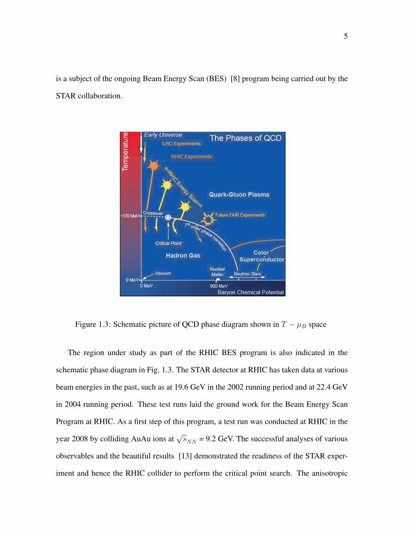
Figure 1.3: Schematic picture of QCD phase diagram shown in T − µB space

The region under study as part of the RHIC BES program is also indicated in the

schematic phase diagram in Fig. 1.3. The STAR detector at RHIC has taken data at various

beam energies in the past, such as at 19.6 GeV in the 2002 running period and at 22.4 GeV

in 2004 running period. These test runs laid the ground work for the Beam Energy Scan

Program at RHIC. As a first step of this program, a test run was conducted at RHIC in the

year 2008 by colliding AuAu ions at√sNN = 9.2 GeV. The successful analyses of various

observables and the beautiful results [13] demonstrated the readiness of the STAR exper-

iment and hence the RHIC collider to perform the critical point search. The anisotropic

6

flow measurements from these test runs are also included in chapter 5 and chapter 6 of this

dissertation.

The main part of the BES phase-one data taking happened successfully in 2010 (Run

10) and 2011(Run 11). STAR took data at√sNN=7.7, 11.5 and 39 GeV in the year 2010

and at√sNN =19.6 and 27 GeV in the year 2011. The corresponding µB coverage of these

energies is estimated to be 112 < µB < 410 MeV. Anisotropic flow analysis of these data

is one of the main objectives of this dissertation.

1.4 Physics Observables for RHIC Energy Scan

The most important physics observables identified for the BES program are broadly

classified into two groups [8]. The first group of observables is studied to search for “turn-

off” of the QGP signatures already established at the top RHIC energies as we scan down

in beam energy. The second group of observables has promise in the search for a first-order

phase transition and for a critical point. Some selected observables are reviewed below.

1.4.1 QGP Signatures

It is generally recognized that there is no single unique signal which allows an unequiv-

ocal identification of quark-gluon plasma. Here we discuss some of the observables which

may strengthen evidence for the presence of the de-confined phase.

Number of Constituent-Quark (NCQ) Scaling of v2

The azimuthal distribution of particles with respect to the reaction plane allows a mea-

surement of anisotropic flow and it is conveniently characterized by the Fourier coefficients

[14]

vn = 〈cosn(φ−Ψr)〉 (1.1)

7

where the angle brackets indicate an average over all the particles used, φ denotes the

azimuthal angle of an outgoing particle, n denotes the Fourier harmonic, and Ψr is the

azimuth of the reaction plane. The reaction plane is defined by the beam axis and the

vector connecting the centers of the two colliding nuclei. Elliptic flow, v2, is the second

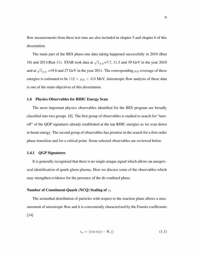
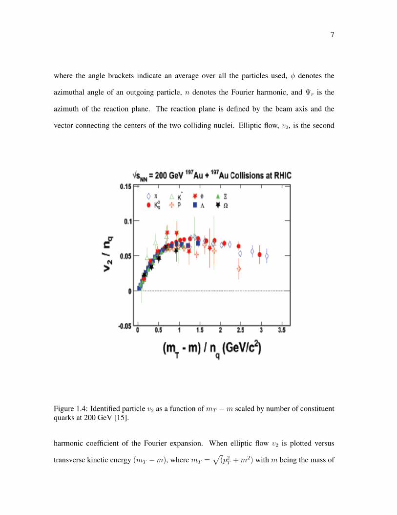
Figure 1.4: Identified particle v2 as a function of mT −m scaled by number of constituentquarks at 200 GeV [15].

harmonic coefficient of the Fourier expansion. When elliptic flow v2 is plotted versus

transverse kinetic energy (mT −m), where mT =√

(p2T +m2) with m being the mass of

8

the particle, v2 for all identified particles below mT −m = 0.9 GeV/c2 falls on a universal

curve. Above that, meson and baryon v2 deviates, with baryon v2 rising above meson v2 and

saturating at a value approximately 50 % larger than for mesons; however, upon dividing

each axis by the number of constituent quarks (nq = 2 for mesons and 3 for baryons), the

meson and baryon curves merge very impressively into a single curve over a wide range of

mT −m. This well-known scaling behavior is one of the most striking pieces of evidence

for the existence of partonic degrees of freedom during the AuAu collision process at 62.4

and 200 GeV [15]. An observation of this NCQ scaling behavior turning off below some

threshold beam energy would be a very powerful confirmation of our current understanding

of the de-confined phase. Elliptic flow will be discussed in detail in the second chapter.

High and Intermediate pT Spectra

High transverse momentum (pT ) particles, emerging from hard scatterings, encounter

energy loss and angular deflection while traversing and interacting with the medium pro-

duced in heavy-ion collisions. The stopping power of a QGP is predicted to be higher

than that of hadronic matter, and this results in jet quenching — a suppressions of high

pT hadron yield relative to the expectation from p+p collisions scaled by the number of

elementary nucleon-nucleon interaction [16].

RAA(pT ) =d2NAA/dpTdy

TAAd2σpp/dpTdy(1.2)

where TAA = 〈Nbin〉/σinelpp is the nucleus overlap function calculated from a Glauber model

[17].

Instead of normalizing the AA spectra with respect to reference pp spectra (which are

not always available), an alternative ratio involves normalizing instead by spectra measured

9

.

Figure 1.5: Left panel: Nuclear Modification Factor RAA as a function of transverse mo-mentum. Right panel: RCP as a function of transverse momentum. Both plots are fromRef. [8]

in peripheral collisions:

RCP (pT ) =(d2NAA/dpTdη)[central]/Ncoll

(d2NAA/dpTdη)[peripheral]/Ncoll

. (1.3)

In 200 and 62.4 GeV AuAu collisions, the high pT hadrons are strongly suppressed

indicating that the strong jet quenching seen at top RHIC energies may set in somewhere

below 62.4 GeV. The particle type dependence of the nuclear modification factor RAA

shows a dependence on constituent quark number rather than mass, indicating that baryon

yields increase faster with the matter density than meson yields. The energy dependence of

the baryon to meson ratio is a particularly stringent test of models such as the recombina-

tion and coalescence models that rely on the interplay between a falling pT spectrum and

recombination or flow to describe the baryon enhancement [8, 16].

Two particle ∆η and ∆φ correlations

Two-particle correlation studies in ∆φ and ∆η at top RHIC energy reveal a correlation

structure strongly elongated in ∆η at small ∆φ as shown in Fig. 1.6. This structure is

10

φ∆

-3-2

-10

12

3

η∆-1.5

-1-0.5

00.5

11.5

)η

∆ d

φ∆

N/(

d2

d

46

47

48

49

50

51

52

53

-310

Au+Au central3<pt

trig<4 GeV/c

Figure 1.6: Two-particle correlation on ∆η and ∆φ of a central event in 200 GeV AuAucollisions [18] showing the ridge in the left panel and the ridge amplitude as a function ofcentrality on the right.

known as the ridge. The amplitude of this ridge-like correlation rises rapidly, reaches a

maximum, and then falls in the most central collisions.

Models based on Glasma flux tubes and Mach cones [19] tried to explain this ridge

phenomenon with a partial success. Recently, it has been argued that the ridge is a natural

outcome of the higher flow harmonics [20, 21], especially the third harmonic popularly

known as “Triangular Flow”. Analysis of triangular flow (v3) is one of the main topics of

this dissertation.

Local Parity Violation in Strong Interactions

In non-central heavy ion collisions, a large orbital angular momentum vector (L) exists

normal (90◦) to the reaction plane, leading to a very intense localized magnetic field (due to

the net charge of the system). If the system is deconfined, there can be strong parity violat-

ing domains, and different numbers of left- and right-hand quarks, leading to preferential

emission of like-sign charged particles along L. In the azimuthally anisotropic emission of

11

Figure 1.7: Signal associated with local parity violation (LPV) at 200 GeV [22]

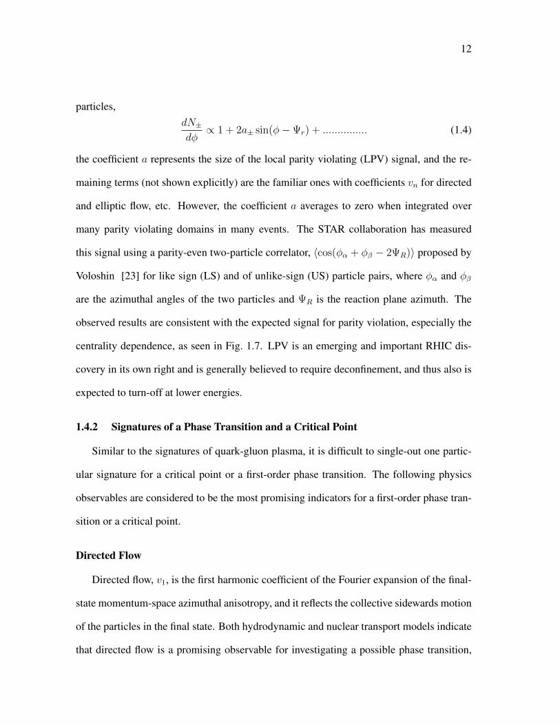
12

particles,dN±dφ∝ 1 + 2a± sin(φ−Ψr) + ............... (1.4)

the coefficient a represents the size of the local parity violating (LPV) signal, and the re-

maining terms (not shown explicitly) are the familiar ones with coefficients vn for directed

and elliptic flow, etc. However, the coefficient a averages to zero when integrated over

many parity violating domains in many events. The STAR collaboration has measured

this signal using a parity-even two-particle correlator, 〈cos(φα + φβ − 2ΨR)〉 proposed by

Voloshin [23] for like sign (LS) and of unlike-sign (US) particle pairs, where φα and φβ

are the azimuthal angles of the two particles and ΨR is the reaction plane azimuth. The

observed results are consistent with the expected signal for parity violation, especially the

centrality dependence, as seen in Fig. 1.7. LPV is an emerging and important RHIC dis-

covery in its own right and is generally believed to require deconfinement, and thus also is

expected to turn-off at lower energies.

1.4.2 Signatures of a Phase Transition and a Critical Point

Similar to the signatures of quark-gluon plasma, it is difficult to single-out one partic-

ular signature for a critical point or a first-order phase transition. The following physics

observables are considered to be the most promising indicators for a first-order phase tran-

sition or a critical point.

Directed Flow

Directed flow, v1, is the first harmonic coefficient of the Fourier expansion of the final-

state momentum-space azimuthal anisotropy, and it reflects the collective sidewards motion

of the particles in the final state. Both hydrodynamic and nuclear transport models indicate

that directed flow is a promising observable for investigating a possible phase transition,

13

especially in the region of relatively low beam energy in the BES range [8]. In particular,

the shape of v1 as a function of rapidity, y, in the midrapidity (|y| < 1.0) region is of interest

because it has been argued that it offers sensitivity to crucial details of the expansion of the

participant matter during the early stages of the collision [24]. I discuss this in detail in the

second chapter.

Fluctuation Measures

Fluctuations are well known phenomena in the context of phase transitions. In particu-

lar, second-order phase transitions are accompanied by fluctuations of the order parameter

at all length scales, leading to phenomena such as critical opalescence [25]. Dynamical

fluctuations in global conserved quantities such as baryon number, strangeness or charge

may be observed near a QCD critical point. The characteristic signature of the existence of

a critical point is an increase, and divergence, of fluctuations [26].

Particle Ratio Fluctuations Particle ratios, e.g. K/π and p/π, probe medium dynamics

at chemical freeze out. They are also convenient to study because volume effects are can-

celed. The beam energy and centrality dependences of the dynamical fluctuations of the

particle ratio may be sensitive to a critical point or a phase transition [27].

Mean pT Fluctuations Average transverse momentum fluctuations are discussed in the

literature in the context of a search for the QCD critical point. It is expected that close to

the critical point, long-range correlations are very strong, resulting in enhanced momentum

fluctuations, especially for small momenta. Small pT values are important because correla-

tion length r diverges at the Critical Point and ∆r∆p ∼ ~/2. In addition to the transverse

momentum fluctuations for all charged particles, one can investigate pT fluctuations of the

negative and positive charges independently, as well as the cross correlations between them.

14

Figure 1.8: Event-wise mean pT distribution for the most central AuAu collisions at 200GeV, measured in the STAR experiment [28]

Fig 1.8 shows the event-wise mean pT distribution in 200 GeV AuAu collisions [28].

Higher Moments and Kurtosis

Due to their high sensitivity to the correlation length and their direct connection to

the thermodynamic susceptibilities, higher moments (Skewness (S), Kurtosis (κ) etc.) of

conserved quantities, such as net-baryons, net-charge and net-strangeness have been ex-

tensively studied to search for the QCD critical point and to probe the bulk properties. It

is expected that the evolution of fluctuations from the critical point to the freeze-out point

may lead to a non-Gaussian shape in the event-by-event multiplicity distributions [29].

The measurement of higher moments of event-by-event identified-particle multiplicity dis-

tributions will provide a direct connection between experimental observables and Lattice

Gauge Theory calculations.

15

Figure 1.9: Energy dependence of moment products κσ2 and Sσ of net-proton distributionsfor (0-5%) central AuAu collisions a function of beam energy [30].

16

Azimuthally-Sensitive Femtoscopy

The probability of detecting two bosons at small relative momentum is affected by

quantum mechanical interference between their wave functions. The interference effect

depends on the space-time extent of the boson-emitting source. This effect is commonly

known as the Hanbury-Brown Twiss (HBT) effect [31]. One of the main observables that

is believed to be sensitive to the Equation of State is the freeze-out shape of the participant

zone in non-central collisions. In heavy-ion collisions, HBT measurements of particles

emitted from the colliding system yield the longitudinal and transverse radii as well as

the lifetime of the emitting source at the moment of thermal freeze-out. Azimuthally-

sensitive femtoscopy adds to the standard HBT observables by allowing the tilt angle of

the ellipsoid-like particle source in coordinate space to be measured. These measurements

hold promise for identifying a softest point, and they complement the momentum-space

information revealed by flow measurements. HBT radii measured relative to the event

plane are the coordinate space analogs of directed and elliptic flow, and are expected to

be sensitive to a softening in the EOS related to a possible first-order phase transition.

The spatial anisotropy probed by HBT is weighted in the time evolution and may retain

sensitivity to the softest point.

1.5 Outline of Current Work

This dissertation is divided into nine chapters. Chapter 2 describes the theory and ap-

plications of anisotropic flow. This chapter also describes some recent experiments similar

to the work reported in this dissertation. Chapter 3 gives a brief description of the STAR

experiment. It describes the various detector subsystems. Chapter 4 describes the analysis

method, with particular emphasis on estimation of the reaction plane based on signals in the

17

Figure 1.10: The transverse spatial freeze out anisotropy ε as a function of collision energy,for midcentral (10-30%) heavy ion collisions [32].

18

Beam Beam Counters (BBC) of the STAR experiment. Use of the BBC for anisotropic flow

measurements is one of the main unique aspects of this PhD project. Chapter 5 presents

the results of directed flow analysis. Chapter 6 presents the results of elliptic flow analysis.

Chapter 7 presents the results of triangular flow analysis and chapter 8 presents the results

of dipole asymmetry measurements. Chapter 9 is devoted to a summary and conclusions.

Chapter 2

ANISOTROPIC FLOW

2.1 Introduction

Figure 2.1: Event anisotropy in spatial and momentum space with respect to the reactionplane.

In a non-central relativistic heavy ion collision, the overlap region of the two nuclei in

the transverse plane has a short axis, which is parallel to the vector connecting the center

of two nuclei, and a long axis perpendicular to it. By convention, this long axis defines the

y direction. The incident beam direction defines the z axis. The x − z plane is called the

reaction plane. The particles which are along the short axis are subject to more pressure

gradient than the particles along the long axis. As a result, anisotropy is developed in the

19

20

final state in momentum space. Anisotropic flow measurements refer to this momentum

anisotropy and they reflect the time-evolution of the pressure gradient generated in the sys-

tem at very early times. Flow provides indirect access to the EOS of the hot and dense

matter formed in the reaction zone, and helps us to understand processes such as thermal-

ization, creation of QGP, phase transitions, etc. It is one of the important measurements

in relativistic heavy-ion collisions and has attracted attention from both theoreticians and

experimentalists [14].

Anisotropic flow is conveniently quantified by the Fourier coefficients of the particle

distribution, written as

Ed3N

d3p=

1

2π

d2N

pTdpTdy(1 +

∞∑n=1

2vn cosnφ). (2.1)

where pT is the transverse momentum, y is rapidity and φ is the angle between each particle

and the true reaction plane angle, ψR, defined by the x − z plane. The sine terms in the

Fourier expansion vanish due to reflection symmetry with respect to the reaction plane. It

follows that 〈cosnφ〉 gives vn, as shown below.

〈cosnφ〉 =

π∫−π

cosnφ E d3Nd3p

dφ∫E d3N

d3pdφ

(2.2)

Substitution from Eq. (2.1) above,

〈cosnφ〉 =

π∫−π

cosnφ (1 +∑∞

n=1 2vn cosnφ)dφ∫(1 +

∑∞n=1 2vn cosnφ)dφ

(2.3)

Now using the orthogonality relation between Fourier coefficients,∫

cosnφ cosmφdφ =

δmn we obtain

21

vn = 〈cosnφ〉. (2.4)

The first three flow components i. e, n = 1, 2 and 3 are called directed flow, elliptic flow

and triangular flow respectively.

2.2 Flow Components

The term directed flow (also called sideward flow) comes from the fact that such a

flow looks like a sideward bounce of the fragments away from each other in the reaction

plane, and the term elliptic flow is inspired by the fact that the azimuthal distribution with a

non-zero second harmonic deviates from isotropic emission in the same way that an ellipse

deviates from a circle. Triangular flow gets its name from a triangular anisotropy in initial

geometry due to fluctuations.

2.2.1 Directed Flow

Directed flow in heavy-ion collisions is quantified by the first harmonic (v1) in the

Fourier expansion of the azimuthal distribution of produced particles with respect to the re-

action plane [14]. It describes collective sideward motion of produced particles and nuclear

fragments and carries information on the very early stages of the collision. The shape of

v1(y) in the central rapidity region is of special interest because it might reveal a signature

of a possible Quark-Gluon Plasma (QGP) phase.

At AGS and lower beam energies, v1 versus rapidity is an almost linear function of ra-

pidity. Often, just the slope of v1(y) at midrapidity is used to define the strength of directed

flow. The sign of v1 is by convention defined as positive for nucleons in the projectile frag-

mentation region [33]. At AGS and lower beam energies, the slope of v1(y) at midrapidity

is observed to be positive for protons, and significantly smaller in magnitude and negative

22

for pions. The opposite directed flow of pions is usually explained in terms of shadowing

by nucleons [34]. At 62.4 and 200 GeV, directed flow is smaller near midrapidity, with a

weaker dependence on rapidity. At these high energies, we observe that the slope of v1 at

midrapidity is negative for nucleons as predicted by models, but pions also have a negative

slope [35]. In one-fluid hydrodynamical calculations, the wiggle structure, i.e., the nega-

tive slope for nucleons, appears only under the assumption of a QGP equation of state, thus

becoming a signature of the QGP phase transition. Then the wiggle structure is interpreted

to be a consequence of the expansion of the highly compressed, disk-shaped system, with

the plane of the disk initially tilted with respect to the beam direction [36]. The subsequent

system expansion leads to the so-called anti-flow or third flow component [38]. Such

flow can reverse the normal pattern of sideward deflection as seen at lower energies, and

hence can result in either a flatness of v1, or a wiggle structure if the expansion is strong

enough. A similar wiggle structure in nucleon v1(y) is predicted if one assumes strong but

incomplete baryon stopping together with strong space-momentum correlations caused by

transverse radial expansion [37].

At energies covered by the RHIC beam energy scan program, the beam rapidity region

lies within STAR detector coverage, and Beam Beam Counters are utilized to reconstruct

the first order event plane. The large pseudorapidity gap between east and west BBC and

between BBC and TPC helps us to minimize the azimuthal correlations not related to reac-

tion plane orientation, the so-called non-flow effects. Furthermore particle identification is

greatly enhanced by the addition of the TOF detector [39], which began operation in 2010.

Identified-particle directed flow, especially for protons and pions, provides new insights.

23

Figure 2.2: Directed flow of pions and protons as a function of rapidity at 40A GeV and158A GeV, as reported by the NA49 Collaboration [40].

24

2.2.2 Elliptic Flow

Elliptic flow is caused by the initial geometric deformation of the reaction region in

the transverse plane. At top RHIC energies, elliptic flow tends to preferentially enhance

momenta along the direction of the smallest spatial extent of the source, and thus the in-

plane (positive) component of elliptic flow dominates. In general, large values of elliptic

flow are considered signatures of hydrodynamic behavior, while smaller signals can have

alternative explanations. The centrality dependence of elliptic flow is of special interest. In

the low density limit (LDL), the mean free path is comparable to, or larger than, the system

size, and the colliding nuclei resemble dilute gases. The final anisotropy in momentum

space depends not only on the initial spatial eccentricity ε (defined below in Eq. 2.6), but

also on the particle density, which affects the number of rescatterings. In this limit, the final

elliptic flow is as below; a more detailed formula in given in Ref. [41].

v2 ∝ε

S

dN

dy(2.5)

where dN/dy characterizes density in the longitudinal direction and S = πRxRy is the

initial transverse area of the overlapping zone, with R2x ≡ 〈x2〉 and R2

x ≡ 〈y2〉 describing

the initial geometry of the system in the x and y directions, respectively. Note that the

x − z axes determine the reaction plane. The averages above include a weighting with

the number of collisions along the beam axis in a wounded nucleon [42] calculation. The

spatial eccentricity, also called standard eccentricity, is defined as

ε =R2y −R2

x

R2x +R2

y

, (2.6)

and for hard spheres is proportional to the impact parameter over a wide range of that

variable.

25

Figure 2.3: v2 per number of constituent quarks nq as a function of pT/nq for variousparticle species from 200 GeV Au+Au minimum bias collisions. The plot is from [15].

26

Because of the event-by-event fluctuations in the participant nucleon position, the ec-

centricity driving elliptic flow in a given event is that defined by the principal axes (x′, y′)

of the distribution of participant nucleons. This participant eccentricity εpart can be written

as

εpart =

√(σ2

y − σ2x)

2 + 4σ2xy

σ2x + σ2

y

, (2.7)

where

σ2x = {x2} − {x}2, σ2

y = {y2} − {y}2, (2.8)

σxy = {xy} − {x}{y}, (2.9)

As follows from the argument above, the elliptic flow increases with particle density.

Eventually, it saturates at the hydro limit. In a hydrodynamic picture, where the mean free

path is much less than the geometrical size of the system, the ratio of v2 to ε is expected to

be approximately constant. The differential momentum anisotropy v2(pT ) is also of inter-

est, especially for different hadron species. Fig. 2.3 shows v2 per number of constituent

quarks (nq) as a function of pT/nq for various particle species. All hadrons, except pions,

lie on the same curve within statistics, and there are plausible reasons to expect the pions to

deviate. This universal scaling behavior lends strong support to the finding that collectivity

is developed in the partonic stage at RHIC [15].

2.2.3 Dipole Asymmetry and Triangular Flow

Recent developments in understanding the initial geometry in heavy-ion collisions points

to a “lumpy” initial state. Event-by-event fluctuations in the initial geometry lead to dipole

asymmetry and triangular anisotropy in azimuthal particle production through the collec-

tive expansion of the medium [20, 43].

27

The dipole asymmetry can be quantified as

ε1eiΦ1 = −〈r

3eiφ〉〈r3〉

(2.10)

where ε1 is dipole anisotropy in the initial position, Φ1 is the steepest direction in the

density distribution, and (r, φ) represent the position and azimuthal angle in a polar coor-

dinate system. Various models based on ideal as well as viscous hydrodynamics or nuclear

transport theory have been used to explain and predict these new flow harmonics and their

correlations with each other. On the experimental side, this area has been gaining interest,

and efforts to measure these observables is in progress. Recently Luzum et al. [44] have

proposed a modified event plane method to study this observable, which suppresses the

conventional directed flow and corrects for the effect of momentum conservation.

Figure 2.4: Energy density distribution in the transverse plane for one event, showing tri-angular anisotropy in the initial geometry. This plot is taken from Ref. [45].

28

Triangular anisotropy can be quantified as

ε3,part =

√(〈r2 cos 3φpart〉2 + 〈r2 sin 3φpart〉2)

〈r2〉(2.11)

Figure 2.5: Flow harmonic coefficients for n = 1, 2, 3, 4, 5 as a function of pT in 200 GeVAuAu collisions at zero impact parameter from a nuclear transport model. The plot is fromRef. [46].

The experimental measurement of these coefficients, i.e., dipole asymmetry and trian-

gular flow, could provide some insight into the initial state geometry fluctuations.

2.3 Flow Fluctuations

Until recently, it was assumed that the event plane azimuth Ψn is completely uniform

and symmetric with respect to the impact parameter for the third and higher-order odd

flow harmonics. This assumption was based on the known symmetry when identical spher-

ical nuclei collide. Now it is realized that event-by-event fluctuations break this symme-

try [20,21,43] and these event-by-event fluctuations lead to dipole asymmetry, triangularity,

and higher-order anisotropy arising from the initial geometry. Flow harmonics associated

with these initial geometry fluctuations carry valuable information about the initial state

29

of the colliding systems and about the hydrodynamic evolution of the fireball created in

the collision. In the Monte Carlo Glauber (MCG) model, the geometric fluctuations of the

positions of nucleons lead to fluctuations of the participant plane from one event to another,

which translates into flow fluctuations for the final-state particles [17]. It has been known

for several years that flow fluctuations are important, but initially only the effect on elliptic

flow v2 was studied [47]. Measurement of flow fluctuations with odd harmonics provides

important clues to understanding the expansion dynamics of the produced fireball and to

quantify the medium properties. Simultaneous knowledge of multiple flow harmonics from

the same system help to constrain the initial parameters [48] in various models describing

heavy-ion collisions. This dissertation reports the first measurement of triangular flow and

the flow harmonic associated with dipole asymmetry from the STAR experiment.

2.4 Non Flow Correlations

Two-particle azimuthal correlations not related to initial geometry or to the reaction

plane are called non-flow [49]. These intrinsic correlations may come from short-range

correlations like Bose-Einstein effects, resonance decays, and Coulomb interactions, or

from jet or minijet correlations. In this study, we focus on discoveries related to initial

geometry and the reaction plane, and therefore non-flow is an unwanted background effect

that can obscure the desired signal. Non-flow effects are difficult to remove from the anal-

ysis, and can lead us astray from the true interpretation of anisotropic flow [49]. Non-flow

limits the precise extraction of the viscosity to entropy density ratio η/s from data-model

comparisons. Isolation of flow and non-flow is critical to the interpretation of the Fourier

decomposition of fluid-like correlations.

Short-range non-flow correlations can be highly suppressed using an event plane re-

constructed in a detector with a large pseudorapidity gap between the event plane and the

30

particles correlated with it. To reduce the sensitivity of our analysis to non-flow effects, we

aim to reconstruct the reaction plane from the charged particles detected by the Beam Beam

Counters (BBC). The large gap of more than two units in pseudorapidity between the TPC

where flow is measured, and the BBC where the event plane is reconstructed, suppresses

most of the non-flow correlations.

2.5 Model Calculations

2.5.1 RQMD

RQMD (Relativistic Quantum Molecular Dynamics) [50] is a semiclassical micro-

scopic transport model, that combines classical propagation with stochastic interactions.

In RQMD, strings and resonances are excited in elementary collisions of nucleons, and

overlapping strings may fuse into “color ropes”. Subsequently, the fragmentation products

from ropes, strings, and resonance decays interact with each other and the original nucle-

ons, mostly via binary collisions. These interactions drive the system towards equilibration

and are responsible for the collective flow development, even in the pre-equilibrium stage.

The RQMD code contains an option to vary the pressure in the high-density stage. In the

medium, baryons may acquire effective masses, generated by introducing Lorentz-invariant

quasipotentials into the mass-shell constraints, which simulate the effect of “mean fields”.

There are no potential-type interactions in the so-called cascade mode of RQMD, where the

equilibrium pressure is simply that of an ideal gas of hadrons and resonances. Its equation

of state is very similar to the one calculated in Ref. [51], because the spectrum of included

resonance states is nearly the same.

While the predictions for baryon directed flow are unambiguous in both hydrodynam-

ical and transport models, the situation for pion directed flow is less clear. RQMD model

31

Figure 2.6: RQMD calculation of v1 (filled circles) and s1 which represents the initialcoordinate-state anisotropy (open circles) for nucleons (left panel) and pions (right panel)in 200 GeV Au+Au collisions [37].

32

calculations for AuAu collisions at√sNN = 200 GeV indicate that shadowing by protons

causes the pions to flow mostly with opposite sign to the protons, but somewhat diffused

due to higher thermal velocities for pions.

RQMD is a microscopic nuclear transport model and does not assume formation of a

QGP. In the simulation shown in Fig. 2.6, the “wiggle” is caused by a combination of space-

momentum correlations characteristic of radial expansion, together with the correlation

between the position of a nucleon in the nucleus and how much rapidity shift it experiences

during the collision [37]. The wiggle predicted by this mechanism appears in peripheral or

mid-peripheral collisions. An investigation of possible wiggle structures at RHIC is among

the important goals of this dissertation.

2.5.2 UrQMD

UrQMD (Ultra-relativistic Quantum Molecular Dynamics) [52] is another relativistic

hadronic transport model describing the phenomenology of nuclear collisions, and grew

out of an effort to improve RQMD and adapt it for higher beam energies. The collision term

is roughly the same as that of RQMD, though some implementation details are improved.

For example, UrQMD handles more types of particles, and employs more detailed cross

sections parametrized according to experimental data. In the early versions of UrQMD,

hard processes are not included.

2.5.3 AMPT

The AMPT model (A Multi-Phase Transport model) [53] is a hybrid model. In the

initial stage, it uses minijet partons from hard processes, and strings from soft processes,

in the heavy ion jet interaction generator (HIJING). The time evolution of the resulting

minijet partons is then described by Zhang’s Parton Cascade (ZPC) model. After minijet

33

partons stop interacting, they are combined with their parent strings, as in the HIJING

model with jet quenching, to fragment into hadrons using the Lund string fragmentation

model as implemented in the PYTHIA program. The final-state hadronic scatterings are

then modeled by ART (A Relativistic Transport model). The AMPT model has a “string

melting” option to convert the initial excited strings into partons. Interactions among these

partons are again described by the ZPC parton cascade model. Since there are no inelastic

scatterings, only quarks and antiquarks from the melted strings are present in the partonic

matter. The transition from partonic matter to hadronic matter is achieved using a simple

coalescence model, where adjacent quark-antiquark pairs are combined into mesons and

likewise, adjacent quark/antiquark triplets with appropriate invariant masses are combined

into baryons/antibaryons.

Chapter 3

EXPERIMENTAL DETAILS

3.1 The Relativistic Heavy Ion Collider

The Relativistic Heavy Ion Collider (RHIC) at Brookhaven National Laboratory (BNL)

is a world-class scientific research facility that began operation in 2000, following 10 years

of development and construction. The Relativistic Heavy Ion Collider complex is actually

composed of several accelerator facilities “chained” together to provide beams which are

collided in detectors located around the RHIC ring.

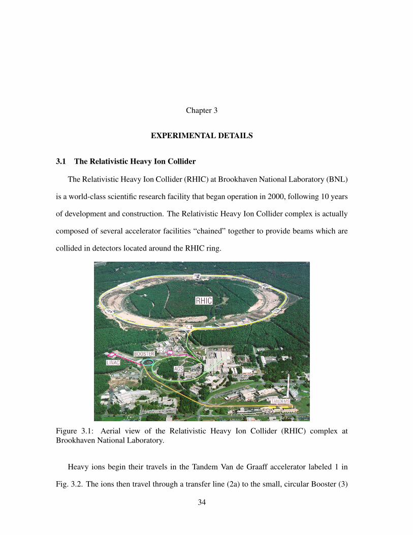
Figure 3.1: Aerial view of the Relativistic Heavy Ion Collider (RHIC) complex atBrookhaven National Laboratory.

Heavy ions begin their travels in the Tandem Van de Graaff accelerator labeled 1 in

Fig. 3.2. The ions then travel through a transfer line (2a) to the small, circular Booster (3)

34

35

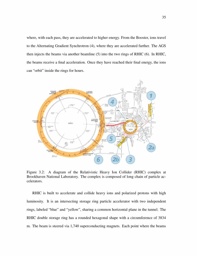
where, with each pass, they are accelerated to higher energy. From the Booster, ions travel

to the Alternating Gradient Synchrotron (4), where they are accelerated further. The AGS

then injects the beams via another beamline (5) into the two rings of RHIC (6). In RHIC,

the beams receive a final acceleration. Once they have reached their final energy, the ions

can “orbit” inside the rings for hours.

Figure 3.2: A diagram of the Relativistic Heavy Ion Collider (RHIC) complex atBrookhaven National Laboratory. The complex is composed of long chain of particle ac-celerators.

RHIC is built to accelerate and collide heavy ions and polarized protons with high

luminosity. It is an intersecting storage ring particle accelerator with two independent

rings, labeled “blue” and “yellow”, sharing a common horizontal plane in the tunnel. The

RHIC double storage ring has a rounded hexagonal shape with a circumference of 3834

m. The beam is steered via 1,740 superconducting magnets. Each point where the beams

36

cross is an interaction point. There are six such locations at RHIC, each described by

a clock position as schematically shown in Fig. 3.2. STAR and PHENIX, the only two

detectors in operation at the time of writing this dissertation, are located at intersection

points corresponding to the 6 o’clock and 8 o’clock positions, respectively. PHOBOS and

BRAHMS, located at the 10 o’clock and 2 o’clock positions respectively, are no longer in

operation. The remaining two collisions points are for possible expansion.

Given below is a brief introduction to the main features of the STAR detector system at

RHIC.

3.2 The STAR Detector

The layout of the STAR detector [54] is shown in Fig. 3.3. STAR was designed pri-

marily for measurements of hadron production over a large solid angle, featuring detector

systems for high precision tracking, momentum analysis, and particle identification opti-

mized for the center of mass (c.m.) rapidity region. It consists of several types of detectors,

each specializing in detecting certain types of particles or characterizing their motion. Data

from these detectors are recorded by an advanced data acquisition (DAQ) system. The

main detector subsystems are: Time Projection Chamber (TPC), Forward Time Projection

Chamber (FTPC), Time of Flight (ToF), Beam-Beam Counters (BBC), Vertex Position De-

tector (VPD), Photon Multiplicity Detector (PMD), Forward Pion Detector (FPD), Barrel

Electro-Magnetic Calorimeter (BEMC), Endcap Electro-Magnetic Calorimeter (EEMC)

and Zero Degree Calorimeter (ZDC). Fig. 3.4 shows the cross-section of the STAR detec-

tors used in the year 2010.

In the analysis for this dissertation, I only used the Time Projection Chamber (TPC),

the Forward TPCs (FTPC), Beam Beam Counters (BBC), Vertex Position Detector (VPD),

Time of flight detector (TOF) and Zero Degree Calorimeter (ZDC). The TPC was used for

37

Figure 3.3: The STAR detector systems showing the location of the detector subsystems.

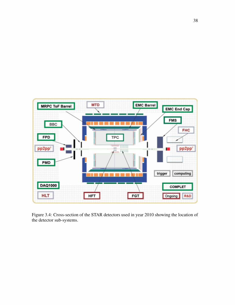
38

Figure 3.4: Cross-section of the STAR detectors used in year 2010 showing the location ofthe detector sub-systems.

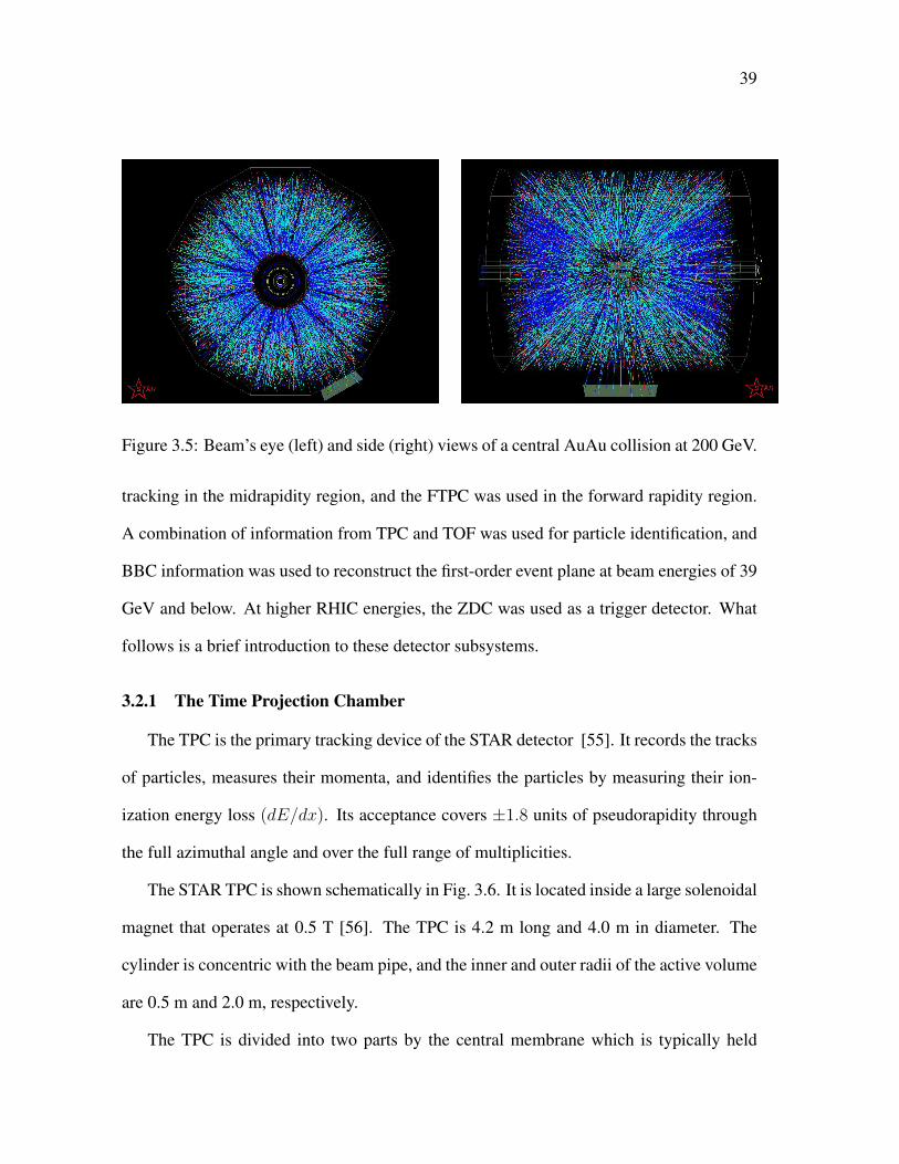
39

Figure 3.5: Beam’s eye (left) and side (right) views of a central AuAu collision at 200 GeV.

tracking in the midrapidity region, and the FTPC was used in the forward rapidity region.

A combination of information from TPC and TOF was used for particle identification, and

BBC information was used to reconstruct the first-order event plane at beam energies of 39

GeV and below. At higher RHIC energies, the ZDC was used as a trigger detector. What

follows is a brief introduction to these detector subsystems.

3.2.1 The Time Projection Chamber

The TPC is the primary tracking device of the STAR detector [55]. It records the tracks

of particles, measures their momenta, and identifies the particles by measuring their ion-

ization energy loss (dE/dx). Its acceptance covers ±1.8 units of pseudorapidity through

the full azimuthal angle and over the full range of multiplicities.

The STAR TPC is shown schematically in Fig. 3.6. It is located inside a large solenoidal

magnet that operates at 0.5 T [56]. The TPC is 4.2 m long and 4.0 m in diameter. The

cylinder is concentric with the beam pipe, and the inner and outer radii of the active volume

are 0.5 m and 2.0 m, respectively.

The TPC is divided into two parts by the central membrane which is typically held

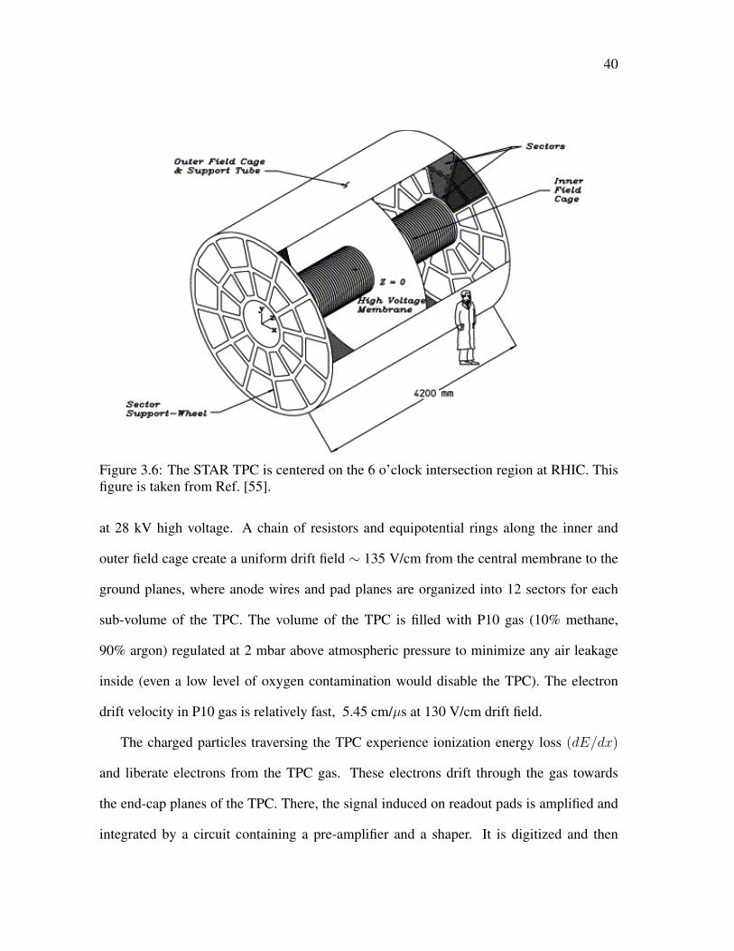
40

Figure 3.6: The STAR TPC is centered on the 6 o’clock intersection region at RHIC. Thisfigure is taken from Ref. [55].

at 28 kV high voltage. A chain of resistors and equipotential rings along the inner and

outer field cage create a uniform drift field ∼ 135 V/cm from the central membrane to the

ground planes, where anode wires and pad planes are organized into 12 sectors for each

sub-volume of the TPC. The volume of the TPC is filled with P10 gas (10% methane,

90% argon) regulated at 2 mbar above atmospheric pressure to minimize any air leakage

inside (even a low level of oxygen contamination would disable the TPC). The electron

drift velocity in P10 gas is relatively fast, 5.45 cm/µs at 130 V/cm drift field.

The charged particles traversing the TPC experience ionization energy loss (dE/dx)

and liberate electrons from the TPC gas. These electrons drift through the gas towards

the end-cap planes of the TPC. There, the signal induced on readout pads is amplified and

integrated by a circuit containing a pre-amplifier and a shaper. It is digitized and then

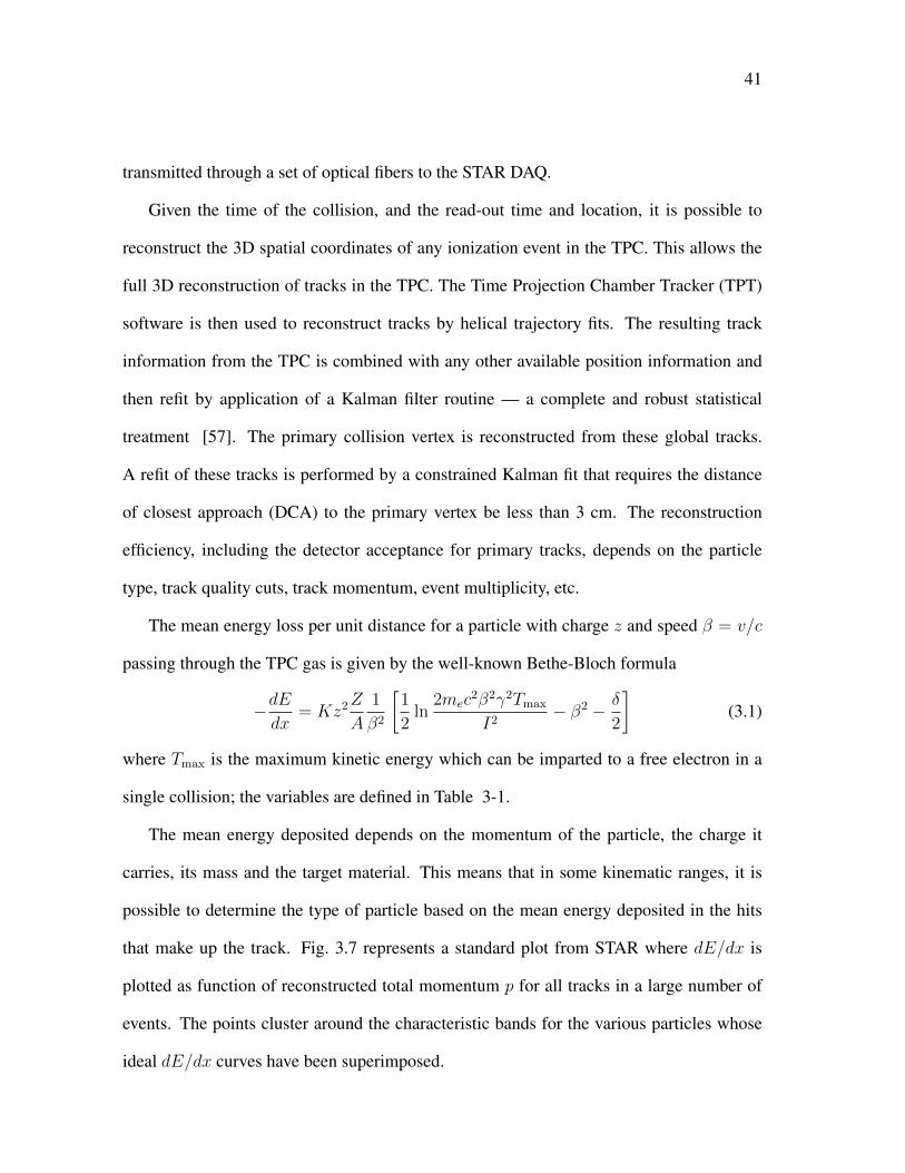
41

transmitted through a set of optical fibers to the STAR DAQ.

Given the time of the collision, and the read-out time and location, it is possible to

reconstruct the 3D spatial coordinates of any ionization event in the TPC. This allows the

full 3D reconstruction of tracks in the TPC. The Time Projection Chamber Tracker (TPT)

software is then used to reconstruct tracks by helical trajectory fits. The resulting track

information from the TPC is combined with any other available position information and

then refit by application of a Kalman filter routine — a complete and robust statistical

treatment [57]. The primary collision vertex is reconstructed from these global tracks.

A refit of these tracks is performed by a constrained Kalman fit that requires the distance

of closest approach (DCA) to the primary vertex be less than 3 cm. The reconstruction

efficiency, including the detector acceptance for primary tracks, depends on the particle

type, track quality cuts, track momentum, event multiplicity, etc.

The mean energy loss per unit distance for a particle with charge z and speed β = v/c

passing through the TPC gas is given by the well-known Bethe-Bloch formula

−dEdx

= Kz2Z

A

1

β2

[1

2ln

2mec2β2γ2Tmax

I2− β2 − δ

2

](3.1)

where Tmax is the maximum kinetic energy which can be imparted to a free electron in a

single collision; the variables are defined in Table 3-1.

The mean energy deposited depends on the momentum of the particle, the charge it

carries, its mass and the target material. This means that in some kinematic ranges, it is

possible to determine the type of particle based on the mean energy deposited in the hits

that make up the track. Fig. 3.7 represents a standard plot from STAR where dE/dx is

plotted as function of reconstructed total momentum p for all tracks in a large number of

events. The points cluster around the characteristic bands for the various particles whose

ideal dE/dx curves have been superimposed.

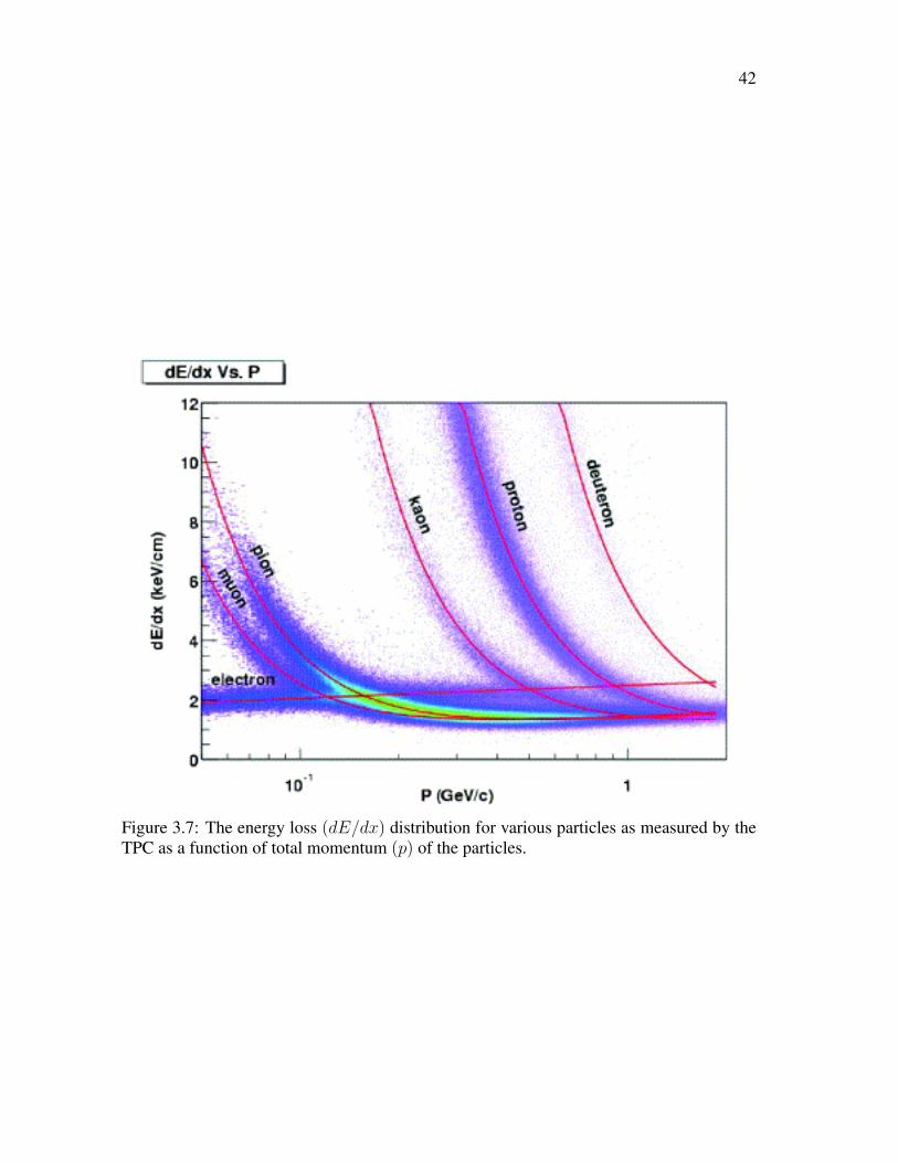
42

Figure 3.7: The energy loss (dE/dx) distribution for various particles as measured by theTPC as a function of total momentum (p) of the particles.

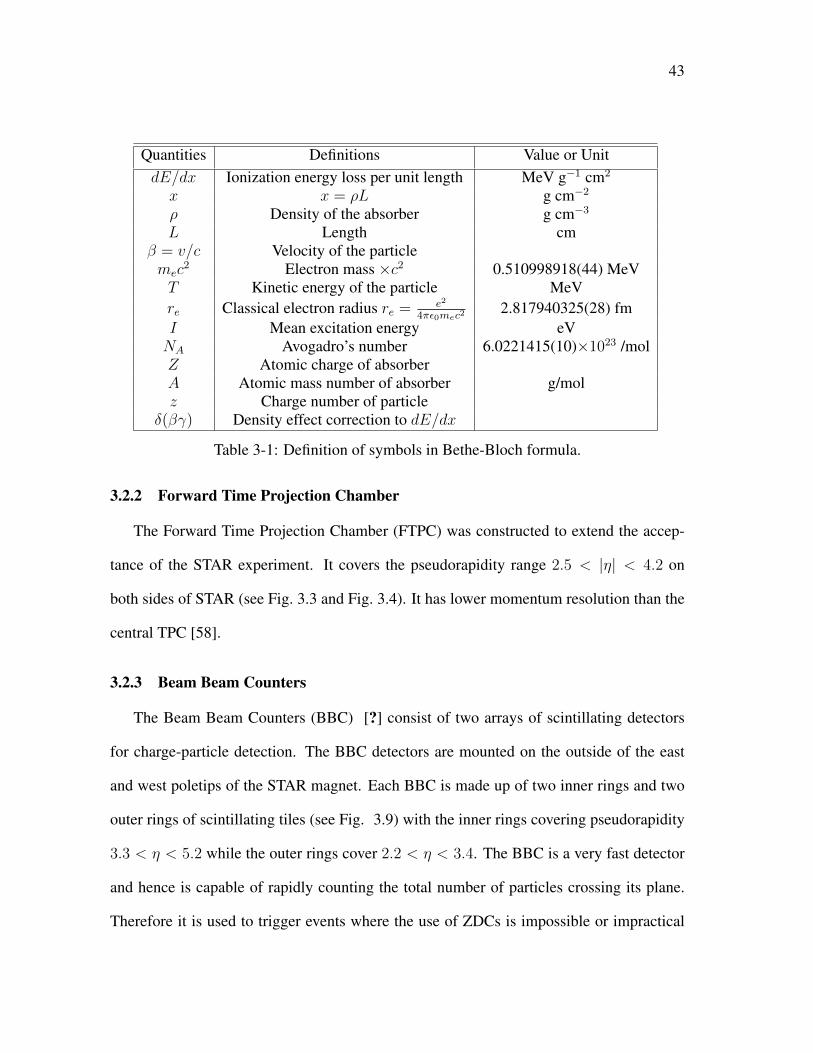
43

Quantities Definitions Value or UnitdE/dx Ionization energy loss per unit length MeV g−1 cm2

x x = ρL g cm−2

ρ Density of the absorber g cm−3

L Length cmβ = v/c Velocity of the particlemec

2 Electron mass ×c2 0.510998918(44) MeVT Kinetic energy of the particle MeVre Classical electron radius re = e2

4πε0mec22.817940325(28) fm

I Mean excitation energy eVNA Avogadro’s number 6.0221415(10)×1023 /molZ Atomic charge of absorberA Atomic mass number of absorber g/molz Charge number of particle

δ(βγ) Density effect correction to dE/dx

Table 3-1: Definition of symbols in Bethe-Bloch formula.

3.2.2 Forward Time Projection Chamber

The Forward Time Projection Chamber (FTPC) was constructed to extend the accep-

tance of the STAR experiment. It covers the pseudorapidity range 2.5 < |η| < 4.2 on

both sides of STAR (see Fig. 3.3 and Fig. 3.4). It has lower momentum resolution than the

central TPC [58].

3.2.3 Beam Beam Counters

The Beam Beam Counters (BBC) [?] consist of two arrays of scintillating detectors

for charge-particle detection. The BBC detectors are mounted on the outside of the east

and west poletips of the STAR magnet. Each BBC is made up of two inner rings and two

outer rings of scintillating tiles (see Fig. 3.9) with the inner rings covering pseudorapidity

3.3 < η < 5.2 while the outer rings cover 2.2 < η < 3.4. The BBC is a very fast detector

and hence is capable of rapidly counting the total number of particles crossing its plane.

Therefore it is used to trigger events where the use of ZDCs is impossible or impractical

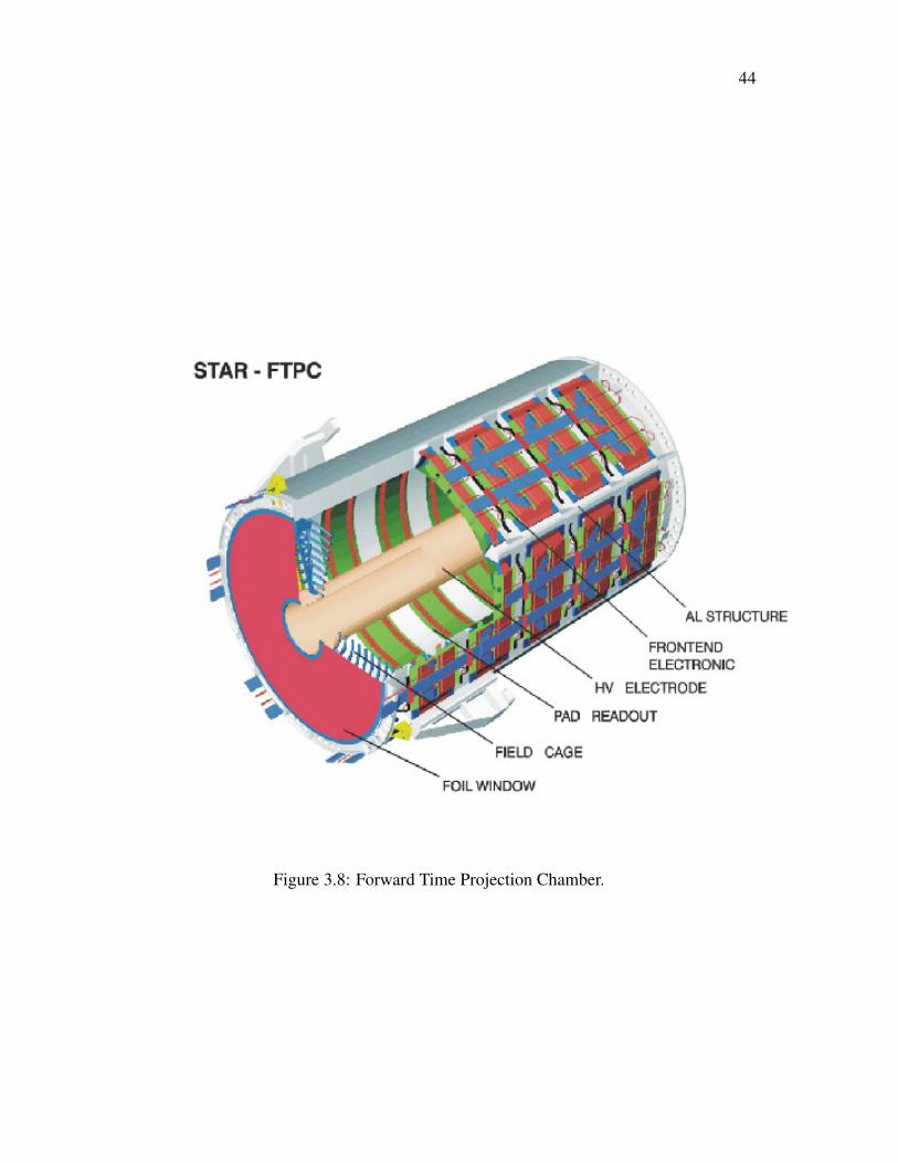
44

Figure 3.8: Forward Time Projection Chamber.

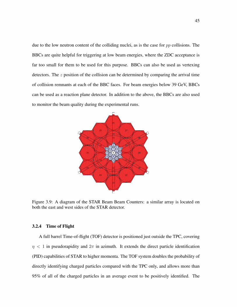
45

due to the low neutron content of the colliding nuclei, as is the case for pp collisions. The

BBCs are quite helpful for triggering at low beam energies, where the ZDC acceptance is

far too small for them to be used for this purpose. BBCs can also be used as vertexing

detectors. The z position of the collision can be determined by comparing the arrival time

of collision remnants at each of the BBC faces. For beam energies below 39 GeV, BBCs

can be used as a reaction plane detector. In addition to the above, the BBCs are also used

to monitor the beam quality during the experimental runs.

Figure 3.9: A diagram of the STAR Beam Beam Counters: a similar array is located onboth the east and west sides of the STAR detector.

3.2.4 Time of Flight

A full barrel Time-of-flight (TOF) detector is positioned just outside the TPC, covering

η < 1 in pseudorapidity and 2π in azimuth. It extends the direct particle identification

(PID) capabilities of STAR to higher momenta. The TOF system doubles the probability of

directly identifying charged particles compared with the TPC only, and allows more than

95% of all of the charged particles in an average event to be positively identified. The

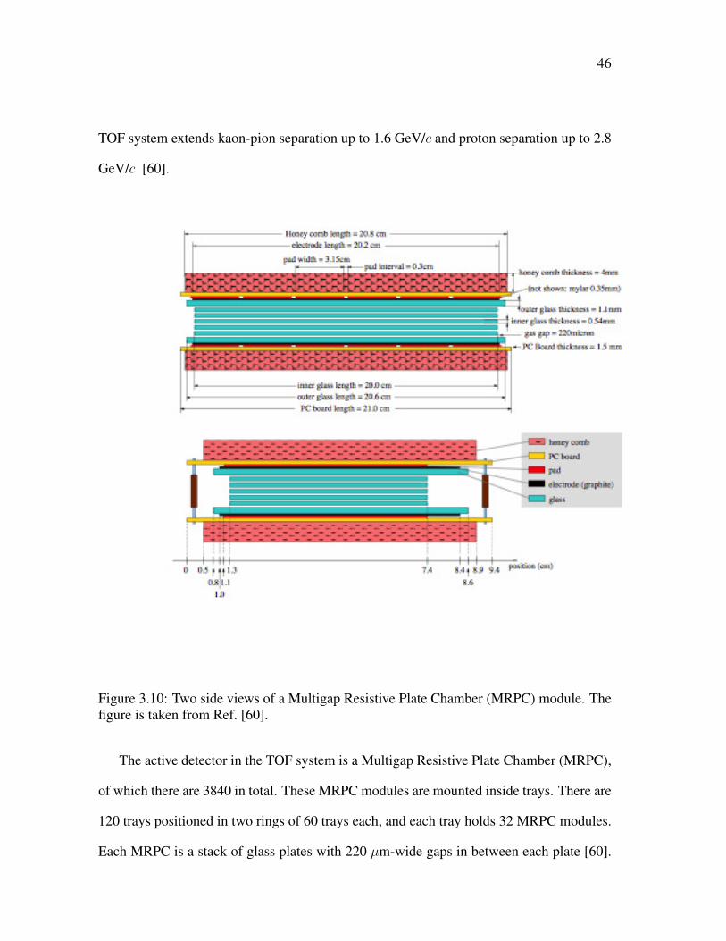
46

TOF system extends kaon-pion separation up to 1.6 GeV/c and proton separation up to 2.8

GeV/c [60].

Figure 3.10: Two side views of a Multigap Resistive Plate Chamber (MRPC) module. Thefigure is taken from Ref. [60].

The active detector in the TOF system is a Multigap Resistive Plate Chamber (MRPC),

of which there are 3840 in total. These MRPC modules are mounted inside trays. There are

120 trays positioned in two rings of 60 trays each, and each tray holds 32 MRPC modules.

Each MRPC is a stack of glass plates with 220 µm-wide gaps in between each plate [60].

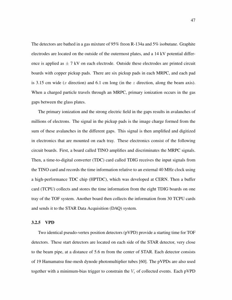
47

The detectors are bathed in a gas mixture of 95% freon R-134a and 5% isobutane. Graphite

electrodes are located on the outside of the outermost plates, and a 14 kV potential differ-

ence is applied as ± 7 kV on each electrode. Outside these electrodes are printed circuit

boards with copper pickup pads. There are six pickup pads in each MRPC, and each pad

is 3.15 cm wide (x direction) and 6.1 cm long (in the z direction, along the beam axis).

When a charged particle travels through an MRPC, primary ionization occurs in the gas

gaps between the glass plates.

The primary ionization and the strong electric field in the gaps results in avalanches of

millions of electrons. The signal in the pickup pads is the image charge formed from the

sum of these avalanches in the different gaps. This signal is then amplified and digitized

in electronics that are mounted on each tray. These electronics consist of the following

circuit boards. First, a board called TINO amplifies and discriminates the MRPC signals.

Then, a time-to-digital converter (TDC) card called TDIG receives the input signals from

the TINO card and records the time information relative to an external 40 MHz clock using

a high-performance TDC chip (HPTDC), which was developed at CERN. Then a buffer

card (TCPU) collects and stores the time information from the eight TDIG boards on one

tray of the TOF system. Another board then collects the information from 30 TCPU cards

and sends it to the STAR Data Acquisition (DAQ) system.

3.2.5 VPD

Two identical pseudo-vertex position detectors (pVPD) provide a starting time for TOF

detectors. These start detectors are located on each side of the STAR detector, very close

to the beam pipe, at a distance of 5.6 m from the center of STAR. Each detector consists

of 19 Hamamatsu fine-mesh dynode photomultiplier tubes [60]. The pVPDs are also used

together with a minimum-bias trigger to constrain the Vz of collected events. Each pVPD

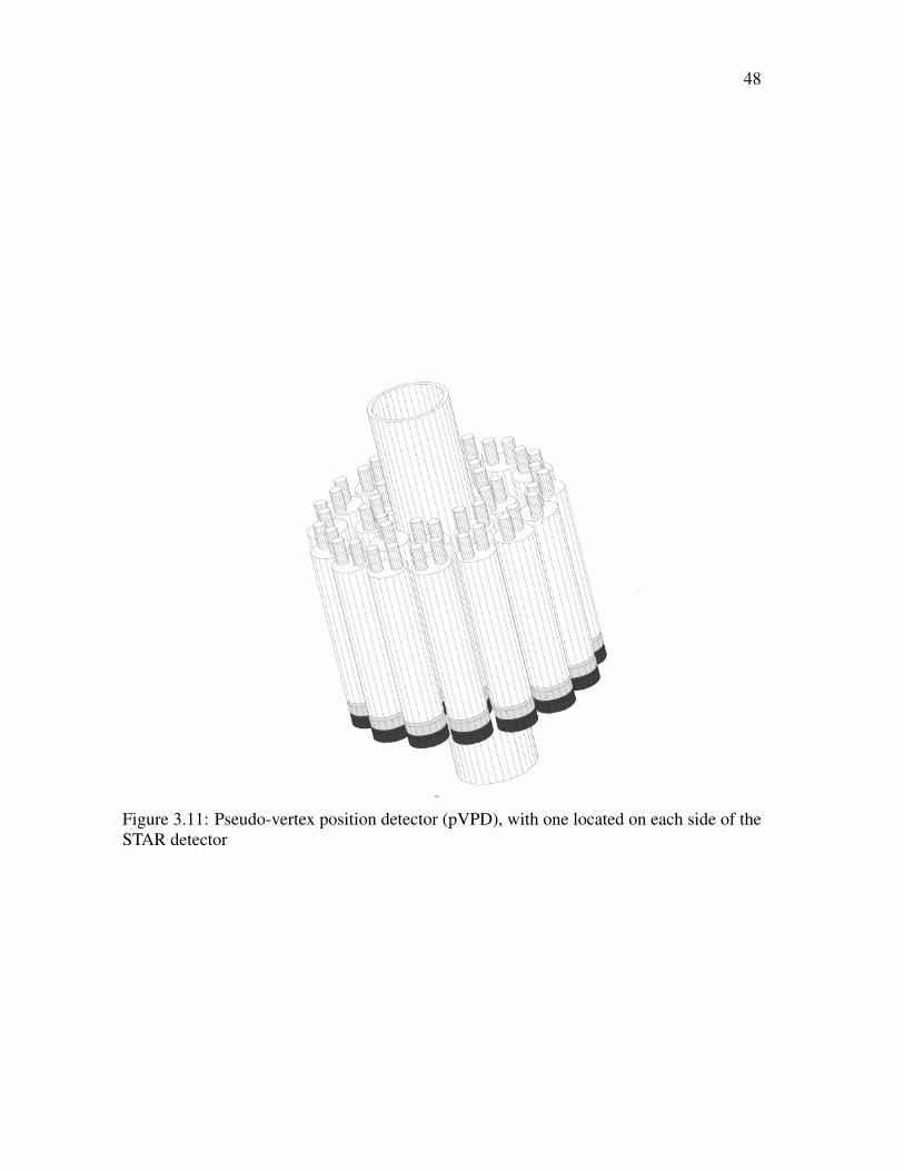
48

Figure 3.11: Pseudo-vertex position detector (pVPD), with one located on each side of theSTAR detector

49

consists of detecting element tubes covering 19% of the total solid angle in 4.43 < |η| <

4.94. The timing resolution of the start time depends on the multiplicity. For example, the

effective timing resolution of the start time is 25 ps, 85 ps, and 140 ps for 200 GeV AuAu,

dAu and pp collisions, respectively.

Figure 3.12: Particle identification using the STAR Time of Flight (TOF) detector. Proton,kaon, pion and electron bands are clearly separated.

3.2.6 ZDC

The Zero Degree Calorimeter (ZDC) is made up of small hadron calorimeters located

downstream (east and west) of the interaction region. The ZDC is placed at≈ 18 m from the

center of STAR and subtends a solid angle of approximately 30µsr. Each ZDC consists of 3

modules containing a series of tungsten plates. The ZDCs measure the energy of neutrons

associated with the spectator matter, and they are used for beam monitoring, triggering and

locating interaction vertices [63, 64].

50

3.2.7 The STAR Trigger

The STAR trigger is a pipelined system in which digitized signals from the fast trigger

detectors are examined at the RHIC crossing rate (∼ 10 MHz). This information is used

to decide whether to begin the amplification-digitization-acquisition cycle for slower, more

finely grained detectors. The slow detectors like the TPC, FTPC, TOF, etc., provide mo-

mentum and particle identification on which physics conclusions are based, but they can

only operate at rates of up to ∼ 1000 Hz (and much slower in the years prior to 2010).

Interaction rates approach the RHIC crossing rates for the highest luminosity beams, so the

fast detectors must provide a means to reduce the rate by up to 5 orders of magnitude. Inter-

actions are, therefore, selected based on the distributions of particles and energy obtained

from the fast trigger detectors, like the BBC, the ZDC, etc.

The trigger system is divided into 4 different levels. The first three levels, 0, 1, and 2,

are based on fast detector information. The final trigger decision is made in level 3 based

on simplified online tracking in the slow detectors. This trigger also provides an online

visual display of the events almost in real time as shown in Fig. 3.5.

The ZDC serves as a main trigger detector at top RHIC energies. BBC and VPD also

serve as trigger detectors, especially for low beam energies where the efficiency of the ZDC

becomes poor.

Chapter 4

ANALYSIS DETAILS

In this chapter, I present the selection criteria for events and tracks, event

plane determination, the analysis methods for directed flow (v1), elliptic flow (v2),

triangular flow (v3) and the first flow harmonic associated with dipole asymmetry

in the initial geometry. I also discuss the estimation of systematic uncertainties on

these measurements.

4.1 Data Sets

Directed flow analysis from the Beam Energy Scan (BES) data set is the main

focus of this dissertation. These data were taken for center of mass energies at 7.7,

11.5 and 39 GeV in the year 2010 and at 19.6 and 27 GeV in the year 2011.

This same data set is analyzed for elliptic flow measurement for charged particles.

Data from low beam energy test runs for AuAu collisions at 9.2 GeV taken in the

year 2008 and for CuCu collisions at 22.4 GeV taken in the year 2005 were also

analyzed for directed and elliptic flow measurements.

The other important component of this dissertation is measurement of triangular

flow and the first flow harmonic associated with dipole asymmetry in the initial

geometry. These odd harmonic coefficients were overlooked until recently and the

first measurement of these observables by the STAR collaboration are reported in

this dissertation. For these measurements, we focused on the data from Au+Au

collisions at 200 GeV from the year 2004. The data with production and trigger

51

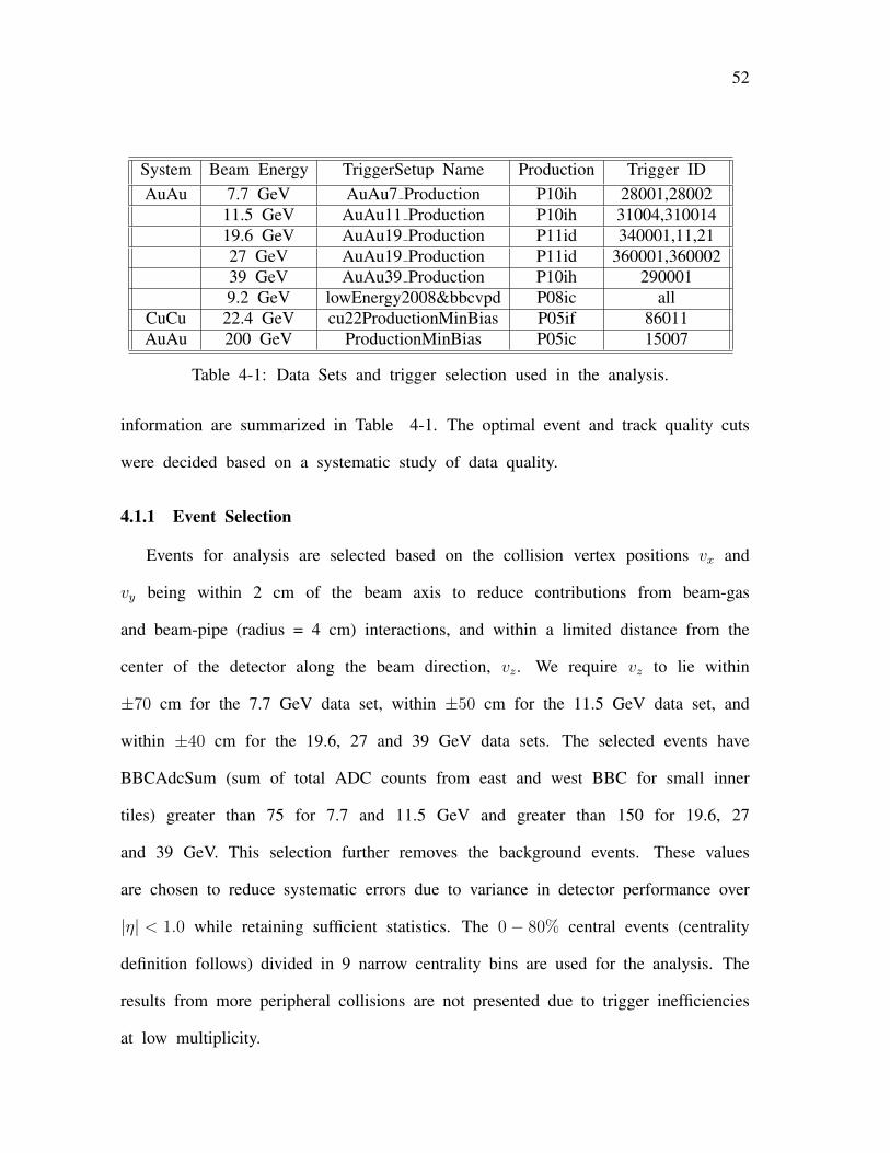
52

System Beam Energy TriggerSetup Name Production Trigger IDAuAu 7.7 GeV AuAu7 Production P10ih 28001,28002

11.5 GeV AuAu11 Production P10ih 31004,31001419.6 GeV AuAu19 Production P11id 340001,11,2127 GeV AuAu19 Production P11id 360001,36000239 GeV AuAu39 Production P10ih 2900019.2 GeV lowEnergy2008&bbcvpd P08ic all

CuCu 22.4 GeV cu22ProductionMinBias P05if 86011AuAu 200 GeV ProductionMinBias P05ic 15007

Table 4-1: Data Sets and trigger selection used in the analysis.

information are summarized in Table 4-1. The optimal event and track quality cuts

were decided based on a systematic study of data quality.

4.1.1 Event Selection

Events for analysis are selected based on the collision vertex positions vx and

vy being within 2 cm of the beam axis to reduce contributions from beam-gas

and beam-pipe (radius = 4 cm) interactions, and within a limited distance from the

center of the detector along the beam direction, vz. We require vz to lie within

±70 cm for the 7.7 GeV data set, within ±50 cm for the 11.5 GeV data set, and

within ±40 cm for the 19.6, 27 and 39 GeV data sets. The selected events have

BBCAdcSum (sum of total ADC counts from east and west BBC for small inner

tiles) greater than 75 for 7.7 and 11.5 GeV and greater than 150 for 19.6, 27

and 39 GeV. This selection further removes the background events. These values

are chosen to reduce systematic errors due to variance in detector performance over

|η| < 1.0 while retaining sufficient statistics. The 0− 80% central events (centrality

definition follows) divided in 9 narrow centrality bins are used for the analysis. The

results from more peripheral collisions are not presented due to trigger inefficiencies

at low multiplicity.

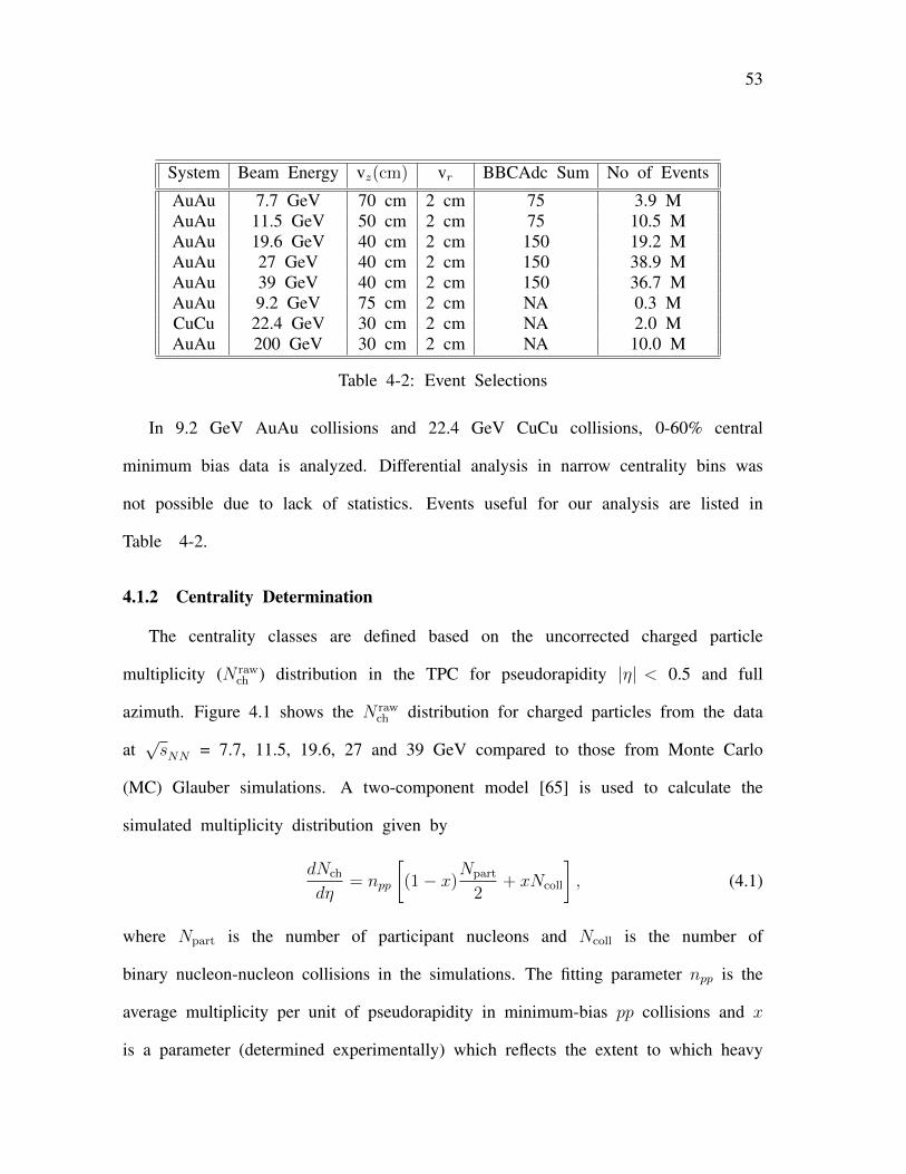
53

System Beam Energy vz(cm) vr BBCAdc Sum No of Events

AuAu 7.7 GeV 70 cm 2 cm 75 3.9 MAuAu 11.5 GeV 50 cm 2 cm 75 10.5 MAuAu 19.6 GeV 40 cm 2 cm 150 19.2 MAuAu 27 GeV 40 cm 2 cm 150 38.9 MAuAu 39 GeV 40 cm 2 cm 150 36.7 MAuAu 9.2 GeV 75 cm 2 cm NA 0.3 MCuCu 22.4 GeV 30 cm 2 cm NA 2.0 MAuAu 200 GeV 30 cm 2 cm NA 10.0 M

Table 4-2: Event Selections

In 9.2 GeV AuAu collisions and 22.4 GeV CuCu collisions, 0-60% central

minimum bias data is analyzed. Differential analysis in narrow centrality bins was

not possible due to lack of statistics. Events useful for our analysis are listed in

Table 4-2.

4.1.2 Centrality Determination

The centrality classes are defined based on the uncorrected charged particle

multiplicity (N rawch ) distribution in the TPC for pseudorapidity |η| < 0.5 and full

azimuth. Figure 4.1 shows the N rawch distribution for charged particles from the data

at√sNN = 7.7, 11.5, 19.6, 27 and 39 GeV compared to those from Monte Carlo

(MC) Glauber simulations. A two-component model [65] is used to calculate the

simulated multiplicity distribution given by

dNch

dη= npp

[(1− x)

Npart

2+ xNcoll

], (4.1)

where Npart is the number of participant nucleons and Ncoll is the number of

binary nucleon-nucleon collisions in the simulations. The fitting parameter npp is the

average multiplicity per unit of pseudorapidity in minimum-bias pp collisions and x

is a parameter (determined experimentally) which reflects the extent to which heavy

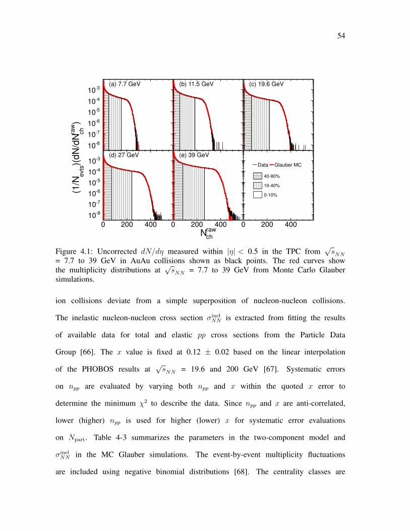
54

810

710

610

510

410

310

810

710

610

510

410

310(a) 7.7 GeV (b) 11.5 GeV (c) 19.6 GeV

rawchN

0 500 1000 1500

810

710

610

510

410

310

0 200 400 0 200 400 0 200 400

810

710

610

510

410

310(d) 27 GeV (e) 39 GeV

Data Glauber MC

4080%

1040%

010%

)ra

w

ch

)(d

N/d

Nevts

(1/N

Figure 4.1: Uncorrected dN/dη measured within |η| < 0.5 in the TPC from√sNN

= 7.7 to 39 GeV in AuAu collisions shown as black points. The red curves showthe multiplicity distributions at

√sNN = 7.7 to 39 GeV from Monte Carlo Glauber

simulations.

ion collisions deviate from a simple superposition of nucleon-nucleon collisions.

The inelastic nucleon-nucleon cross section σinelNN is extracted from fitting the results

of available data for total and elastic pp cross sections from the Particle Data

Group [66]. The x value is fixed at 0.12 ± 0.02 based on the linear interpolation

of the PHOBOS results at√sNN = 19.6 and 200 GeV [67]. Systematic errors

on npp are evaluated by varying both npp and x within the quoted x error to

determine the minimum χ2 to describe the data. Since npp and x are anti-correlated,

lower (higher) npp is used for higher (lower) x for systematic error evaluations

on Npart. Table 4-3 summarizes the parameters in the two-component model and

σinelNN in the MC Glauber simulations. The event-by-event multiplicity fluctuations

are included using negative binomial distributions [68]. The centrality classes are

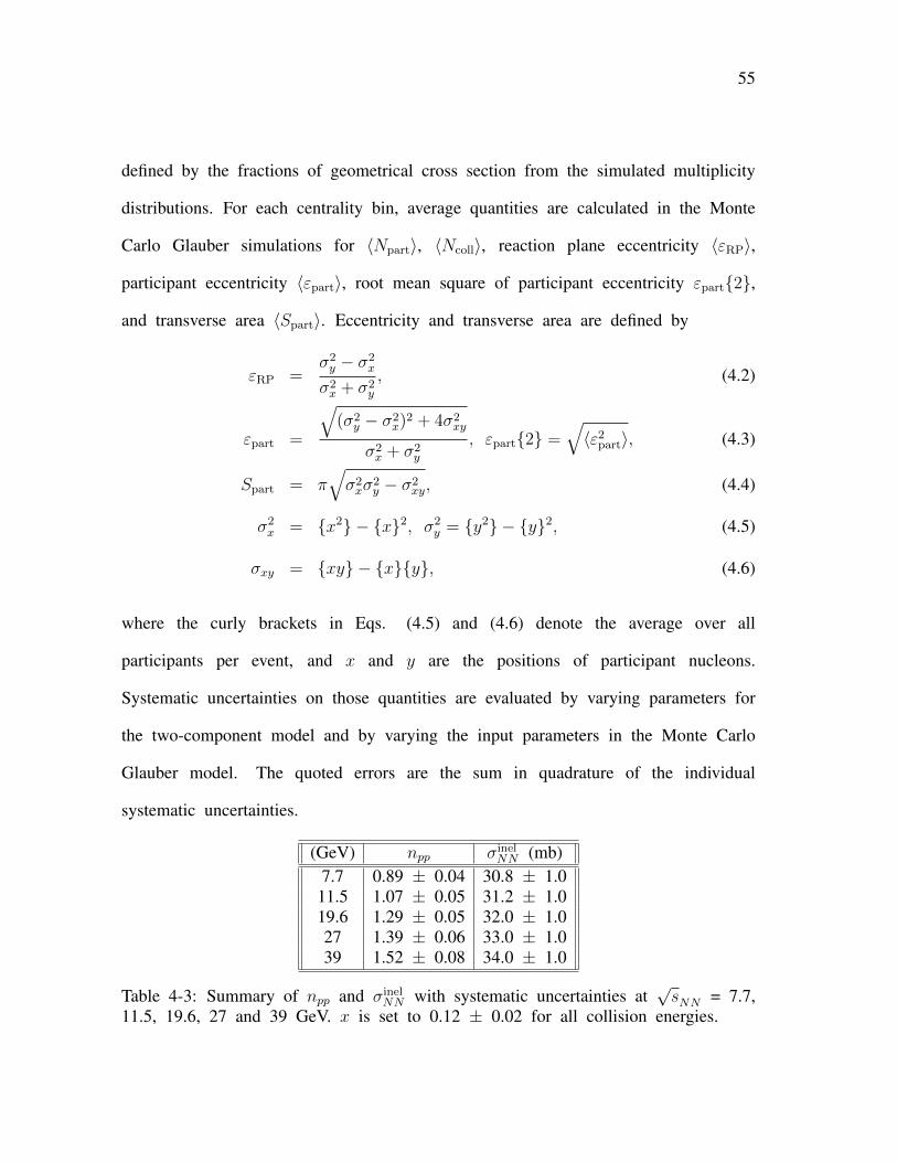
55

defined by the fractions of geometrical cross section from the simulated multiplicity

distributions. For each centrality bin, average quantities are calculated in the Monte

Carlo Glauber simulations for 〈Npart〉, 〈Ncoll〉, reaction plane eccentricity 〈εRP〉,

participant eccentricity 〈εpart〉, root mean square of participant eccentricity εpart{2},

and transverse area 〈Spart〉. Eccentricity and transverse area are defined by

εRP =σ2y − σ2

x

σ2x + σ2

y

, (4.2)

εpart =

√(σ2

y − σ2x)

2 + 4σ2xy

σ2x + σ2

y

, εpart{2} =√〈ε2

part〉, (4.3)

Spart = π√σ2xσ

2y − σ2

xy, (4.4)

σ2x = {x2} − {x}2, σ2

y = {y2} − {y}2, (4.5)

σxy = {xy} − {x}{y}, (4.6)

where the curly brackets in Eqs. (4.5) and (4.6) denote the average over all

participants per event, and x and y are the positions of participant nucleons.

Systematic uncertainties on those quantities are evaluated by varying parameters for

the two-component model and by varying the input parameters in the Monte Carlo

Glauber model. The quoted errors are the sum in quadrature of the individual

systematic uncertainties.

(GeV) npp σinelNN (mb)

7.7 0.89 ± 0.04 30.8 ± 1.011.5 1.07 ± 0.05 31.2 ± 1.019.6 1.29 ± 0.05 32.0 ± 1.027 1.39 ± 0.06 33.0 ± 1.039 1.52 ± 0.08 34.0 ± 1.0

Table 4-3: Summary of npp and σinelNN with systematic uncertainties at

√sNN = 7.7,

11.5, 19.6, 27 and 39 GeV. x is set to 0.12 ± 0.02 for all collision energies.

56

4.1.3 Track Selections

Various track quality cuts are used to select good charged particle tracks

reconstructed using information from the TPC or FTPCs. The distance of closest

approach (DCA) of the track to the primary vertex is taken to be less than 3

cm. We require that in the TPC and FTPCs, the number of fit points used for

reconstruction of the tracks must be greater than 15 and 5, respectively. For the

TPC and FTPCs, the ratio of the number of fit points to the maximum possible

number of points for that trajectory is required to be greater than 0.52. This

requirement prevents a single track being analyzed as two separate tracks if it is

split into two segments during reconstruction. An additional transverse momentum

cut (0.2 < pT < 2 GeV/c) is applied to the charged tracks for the event plane

reconstruction in TPC and FTPC.

4.1.4 Particle Identification

Particles such as protons, pions and kaons can be identified by determining their

mass or the way they interact or decay. The momentum and charge sign of the

charged particles can be determined by measuring the curvature and direction of

the tracks in the detector. To identify hadrons and leptons unambiguously, their

charge and mass have to be determined by measuring the momentum and velocity

simultaneously.

For the data taken in 2010 and later, I use STAR’s new Time of Flight detector

to identify particles in combination with TPC information. The TOF detector

measures flight time of a particle from the primary vertex of the collisions to

the point where the particle crosses the TOF barrel. Once the time of flight and

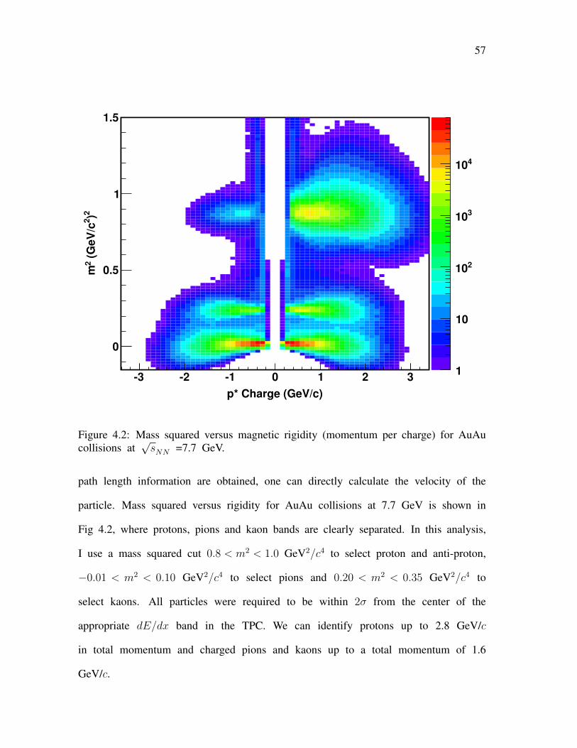
57

p* Charge (GeV/c)

3 2 1 0 1 2 3

2 )2

(G

eV

/c2

m

0

0.5

1

1.5

1

10

210

310

410

Figure 4.2: Mass squared versus magnetic rigidity (momentum per charge) for AuAucollisions at

√sNN =7.7 GeV.

path length information are obtained, one can directly calculate the velocity of the

particle. Mass squared versus rigidity for AuAu collisions at 7.7 GeV is shown in

Fig 4.2, where protons, pions and kaon bands are clearly separated. In this analysis,

I use a mass squared cut 0.8 < m2 < 1.0 GeV2/c4 to select proton and anti-proton,

−0.01 < m2 < 0.10 GeV2/c4 to select pions and 0.20 < m2 < 0.35 GeV2/c4 to

select kaons. All particles were required to be within 2σ from the center of the

appropriate dE/dx band in the TPC. We can identify protons up to 2.8 GeV/c

in total momentum and charged pions and kaons up to a total momentum of 1.6

GeV/c.

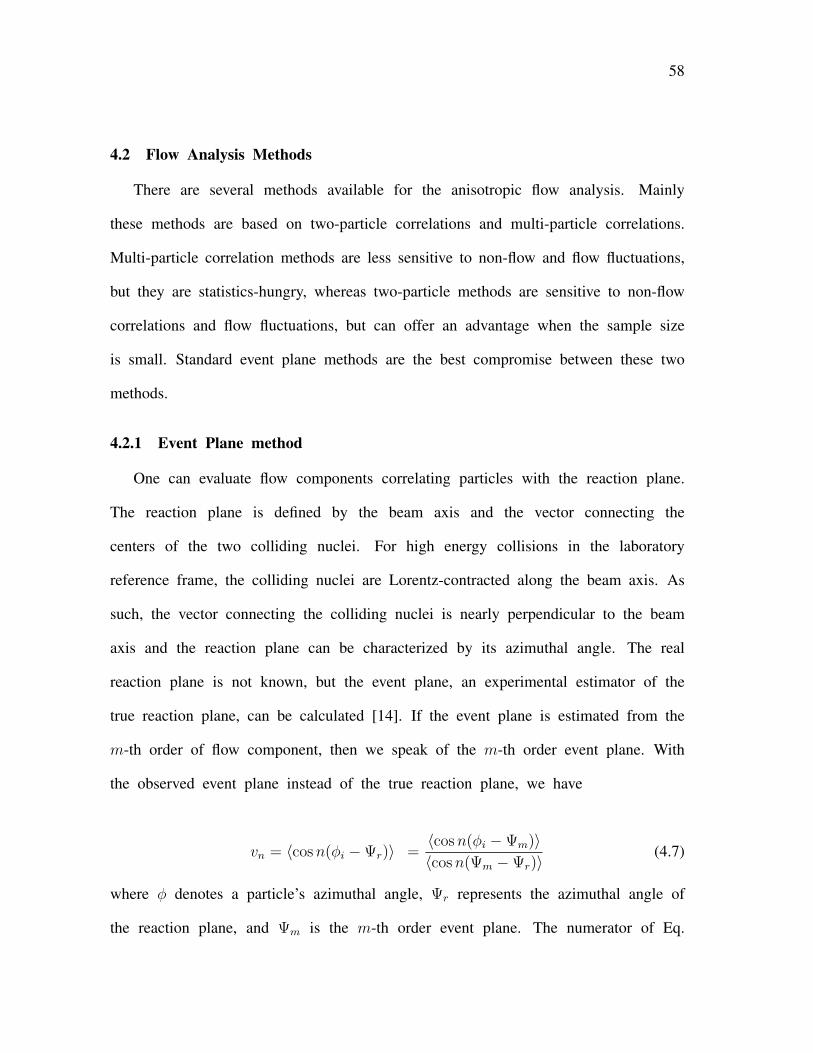
58

4.2 Flow Analysis Methods

There are several methods available for the anisotropic flow analysis. Mainly

these methods are based on two-particle correlations and multi-particle correlations.

Multi-particle correlation methods are less sensitive to non-flow and flow fluctuations,

but they are statistics-hungry, whereas two-particle methods are sensitive to non-flow

correlations and flow fluctuations, but can offer an advantage when the sample size

is small. Standard event plane methods are the best compromise between these two

methods.

4.2.1 Event Plane method

One can evaluate flow components correlating particles with the reaction plane.

The reaction plane is defined by the beam axis and the vector connecting the

centers of the two colliding nuclei. For high energy collisions in the laboratory

reference frame, the colliding nuclei are Lorentz-contracted along the beam axis. As

such, the vector connecting the colliding nuclei is nearly perpendicular to the beam

axis and the reaction plane can be characterized by its azimuthal angle. The real

reaction plane is not known, but the event plane, an experimental estimator of the

true reaction plane, can be calculated [14]. If the event plane is estimated from the

m-th order of flow component, then we speak of the m-th order event plane. With

the observed event plane instead of the true reaction plane, we have

vn = 〈cosn(φi −Ψr)〉 =〈cosn(φi −Ψm)〉〈cosn(Ψm −Ψr)〉

(4.7)

where φ denotes a particle’s azimuthal angle, Ψr represents the azimuthal angle of

the reaction plane, and Ψm is the m-th order event plane. The numerator of Eq.

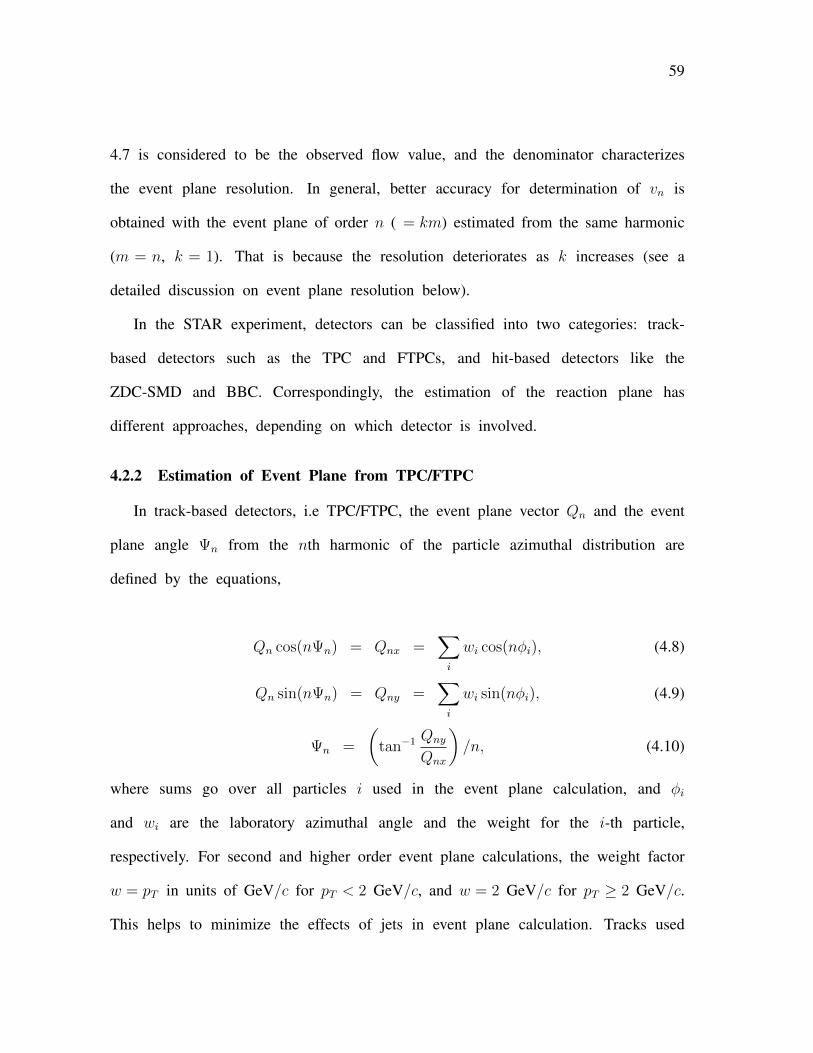
59

4.7 is considered to be the observed flow value, and the denominator characterizes

the event plane resolution. In general, better accuracy for determination of vn is

obtained with the event plane of order n ( = km) estimated from the same harmonic

(m = n, k = 1). That is because the resolution deteriorates as k increases (see a

detailed discussion on event plane resolution below).

In the STAR experiment, detectors can be classified into two categories: track-

based detectors such as the TPC and FTPCs, and hit-based detectors like the

ZDC-SMD and BBC. Correspondingly, the estimation of the reaction plane has

different approaches, depending on which detector is involved.

4.2.2 Estimation of Event Plane from TPC/FTPC

In track-based detectors, i.e TPC/FTPC, the event plane vector Qn and the event

plane angle Ψn from the nth harmonic of the particle azimuthal distribution are

defined by the equations,

Qn cos(nΨn) = Qnx =∑i

wi cos(nφi), (4.8)

Qn sin(nΨn) = Qny =∑i

wi sin(nφi), (4.9)

Ψn =

(tan−1 Qny

Qnx

)/n, (4.10)

where sums go over all particles i used in the event plane calculation, and φi

and wi are the laboratory azimuthal angle and the weight for the i-th particle,

respectively. For second and higher order event plane calculations, the weight factor

w = pT in units of GeV/c for pT < 2 GeV/c, and w = 2 GeV/c for pT ≥ 2 GeV/c.

This helps to minimize the effects of jets in event plane calculation. Tracks used

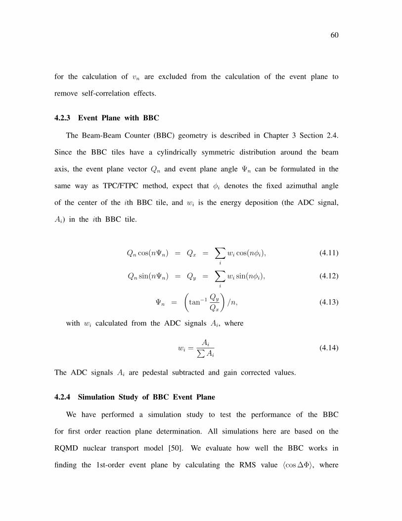
60

for the calculation of vn are excluded from the calculation of the event plane to

remove self-correlation effects.

4.2.3 Event Plane with BBC

The Beam-Beam Counter (BBC) geometry is described in Chapter 3 Section 2.4.

Since the BBC tiles have a cylindrically symmetric distribution around the beam

axis, the event plane vector Qn and event plane angle Ψn can be formulated in the

same way as TPC/FTPC method, expect that φi denotes the fixed azimuthal angle

of the center of the ith BBC tile, and wi is the energy deposition (the ADC signal,

Ai) in the ith BBC tile.

Qn cos(nΨn) = Qx =∑i

wi cos(nφi), (4.11)

Qn sin(nΨn) = Qy =∑i

wi sin(nφi), (4.12)

Ψn =

(tan−1 Qy

Qx

)/n, (4.13)

with wi calculated from the ADC signals Ai, where

wi =Ai∑Ai

(4.14)

The ADC signals Ai are pedestal subtracted and gain corrected values.

4.2.4 Simulation Study of BBC Event Plane

We have performed a simulation study to test the performance of the BBC

for first order reaction plane determination. All simulations here are based on the

RQMD nuclear transport model [50]. We evaluate how well the BBC works in

finding the 1st-order event plane by calculating the RMS value 〈cos ∆Φ〉, where

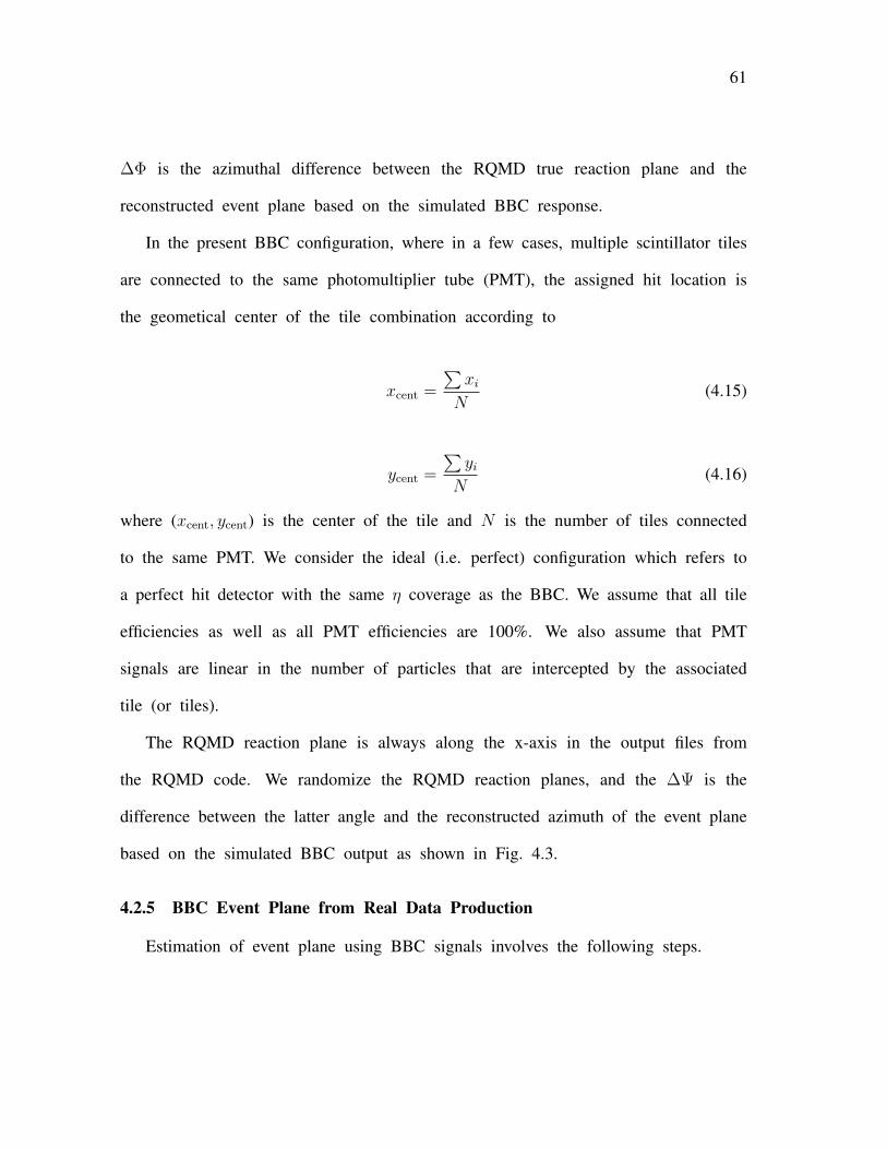
61

∆Φ is the azimuthal difference between the RQMD true reaction plane and the

reconstructed event plane based on the simulated BBC response.

In the present BBC configuration, where in a few cases, multiple scintillator tiles

are connected to the same photomultiplier tube (PMT), the assigned hit location is

the geometical center of the tile combination according to

xcent =

∑xiN

(4.15)

ycent =

∑yi

N(4.16)

where (xcent, ycent) is the center of the tile and N is the number of tiles connected

to the same PMT. We consider the ideal (i.e. perfect) configuration which refers to

a perfect hit detector with the same η coverage as the BBC. We assume that all tile

efficiencies as well as all PMT efficiencies are 100%. We also assume that PMT

signals are linear in the number of particles that are intercepted by the associated

tile (or tiles).

The RQMD reaction plane is always along the x-axis in the output files from

the RQMD code. We randomize the RQMD reaction planes, and the ∆Ψ is the

difference between the latter angle and the reconstructed azimuth of the event plane

based on the simulated BBC output as shown in Fig. 4.3.

4.2.5 BBC Event Plane from Real Data Production

Estimation of event plane using BBC signals involves the following steps.

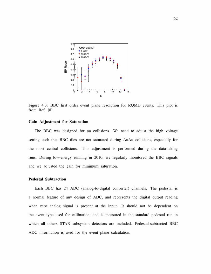
62

b

0 2 4 6 8 10 12 14

EP

Resol

0

0.1

0.2

0.3

0.4

0.5

0.6

0.7

0.8

0.9

RQMD: BBC EP

5 GeV

10 GeV

20 GeV

Figure 4.3: BBC first order event plane resolution for RQMD events. This plot isfrom Ref. [8].

Gain Adjustment for Saturation

The BBC was designed for pp collisions. We need to adjust the high voltage

setting such that BBC tiles are not saturated during AuAu collisions, especially for

the most central collisions. This adjustment is performed during the data-taking

runs. During low-energy running in 2010, we regularly monitored the BBC signals

and we adjusted the gain for minimum saturation.

Pedestal Subtraction

Each BBC has 24 ADC (analog-to-digital converter) channels. The pedestal is

a normal feature of any design of ADC, and represents the digital output reading

when zero analog signal is present at the input. It should not be dependent on

the event type used for calibration, and is measured in the standard pedestal run in

which all others STAR subsystem detectors are included. Pedestal-subtracted BBC

ADC information is used for the event plane calculation.

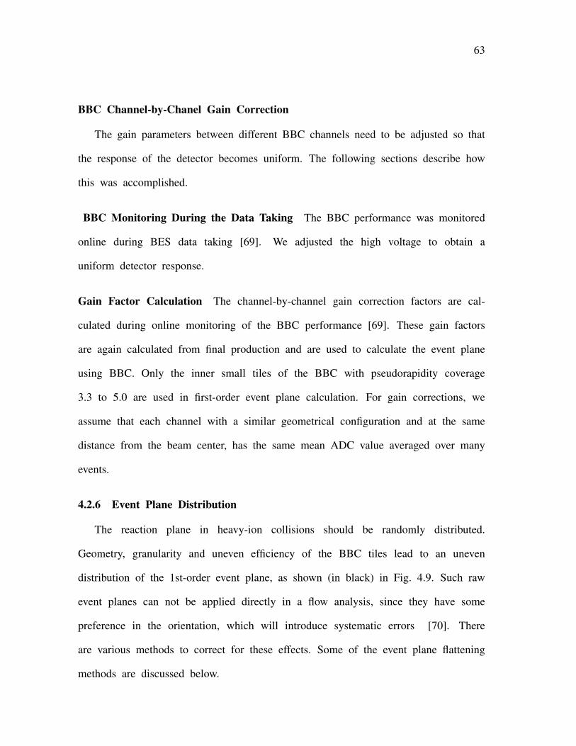
63

BBC Channel-by-Chanel Gain Correction

The gain parameters between different BBC channels need to be adjusted so that

the response of the detector becomes uniform. The following sections describe how

this was accomplished.

BBC Monitoring During the Data Taking The BBC performance was monitored

online during BES data taking [69]. We adjusted the high voltage to obtain a

uniform detector response.

Gain Factor Calculation The channel-by-channel gain correction factors are cal-

culated during online monitoring of the BBC performance [69]. These gain factors

are again calculated from final production and are used to calculate the event plane

using BBC. Only the inner small tiles of the BBC with pseudorapidity coverage

3.3 to 5.0 are used in first-order event plane calculation. For gain corrections, we

assume that each channel with a similar geometrical configuration and at the same

distance from the beam center, has the same mean ADC value averaged over many

events.

4.2.6 Event Plane Distribution

The reaction plane in heavy-ion collisions should be randomly distributed.

Geometry, granularity and uneven efficiency of the BBC tiles lead to an uneven

distribution of the 1st-order event plane, as shown (in black) in Fig. 4.9. Such raw

event planes can not be applied directly in a flow analysis, since they have some

preference in the orientation, which will introduce systematic errors [70]. There

are various methods to correct for these effects. Some of the event plane flattening

methods are discussed below.

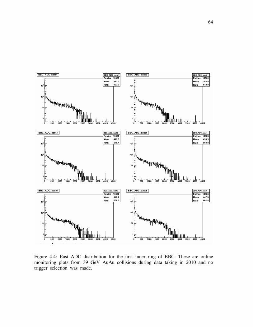
64

Figure 4.4: East ADC distribution for the first inner ring of BBC. These are onlinemonitoring plots from 39 GeV AuAu collisions during data taking in 2010 and notrigger selection was made.

65

Figure 4.5: West ADC distribution for the first inner ring of BBC. These are onlinemonitoring plots from 39 GeV AuAu collisions during data taking in 2010 and notrigger selection was made.

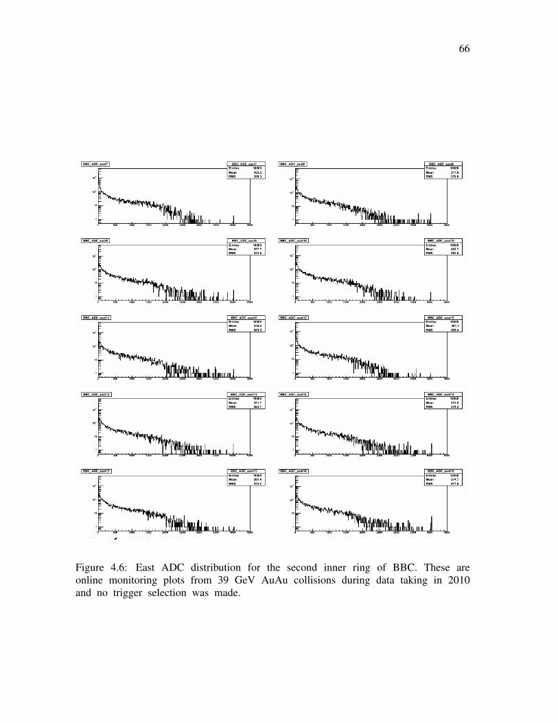
66

Figure 4.6: East ADC distribution for the second inner ring of BBC. These areonline monitoring plots from 39 GeV AuAu collisions during data taking in 2010and no trigger selection was made.

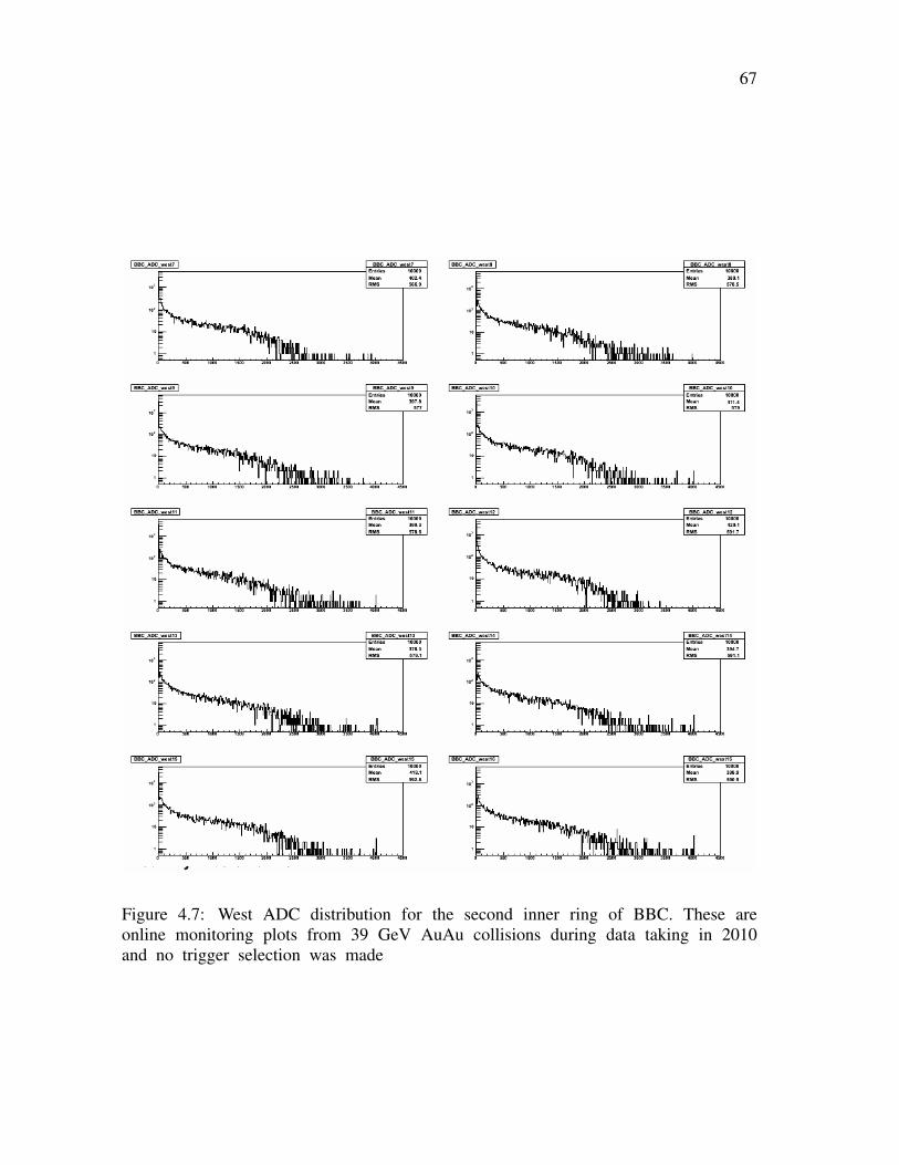
67

Figure 4.7: West ADC distribution for the second inner ring of BBC. These areonline monitoring plots from 39 GeV AuAu collisions during data taking in 2010and no trigger selection was made

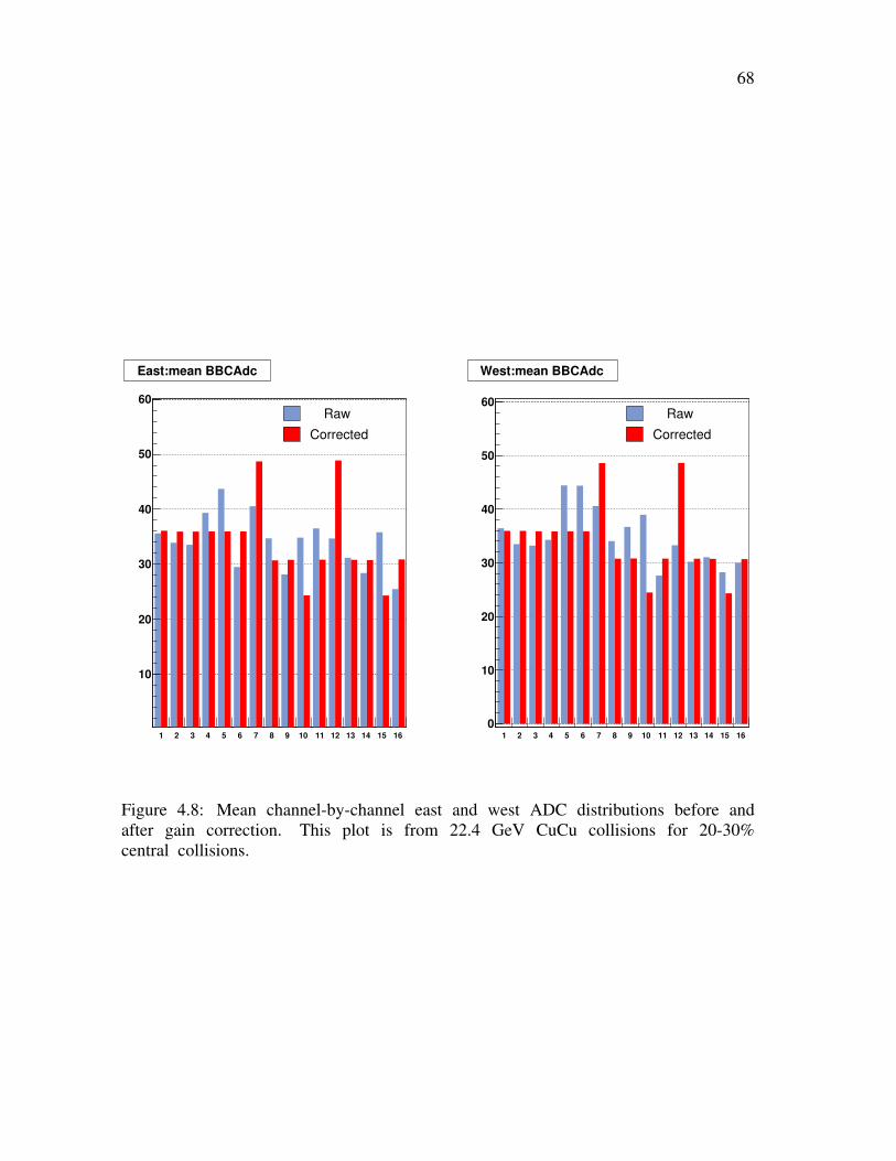
68

1 2 3 4 5 6 7 8 9 10 11 12 13 14 15 16

10

20

30

40

50

60

Raw

Corrected

East:mean BBCAdc

1 2 3 4 5 6 7 8 9 10 11 12 13 14 15 16

0

10

20

30

40

50

60

Raw

Corrected

West:mean BBCAdc

Figure 4.8: Mean channel-by-channel east and west ADC distributions before andafter gain correction. This plot is from 22.4 GeV CuCu collisions for 20-30%central collisions.

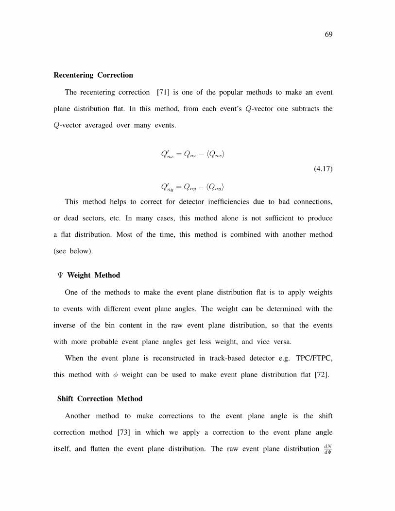
69

Recentering Correction

The recentering correction [71] is one of the popular methods to make an event

plane distribution flat. In this method, from each event’s Q-vector one subtracts the

Q-vector averaged over many events.

Q′nx = Qnx − 〈Qnx〉

Q′ny = Qny − 〈Qny〉

(4.17)

This method helps to correct for detector inefficiencies due to bad connections,

or dead sectors, etc. In many cases, this method alone is not sufficient to produce

a flat distribution. Most of the time, this method is combined with another method

(see below).

Ψ Weight Method

One of the methods to make the event plane distribution flat is to apply weights

to events with different event plane angles. The weight can be determined with the

inverse of the bin content in the raw event plane distribution, so that the events

with more probable event plane angles get less weight, and vice versa.

When the event plane is reconstructed in track-based detector e.g. TPC/FTPC,

this method with φ weight can be used to make event plane distribution flat [72].

Shift Correction Method

Another method to make corrections to the event plane angle is the shift

correction method [73] in which we apply a correction to the event plane angle

itself, and flatten the event plane distribution. The raw event plane distribution dNdΨ

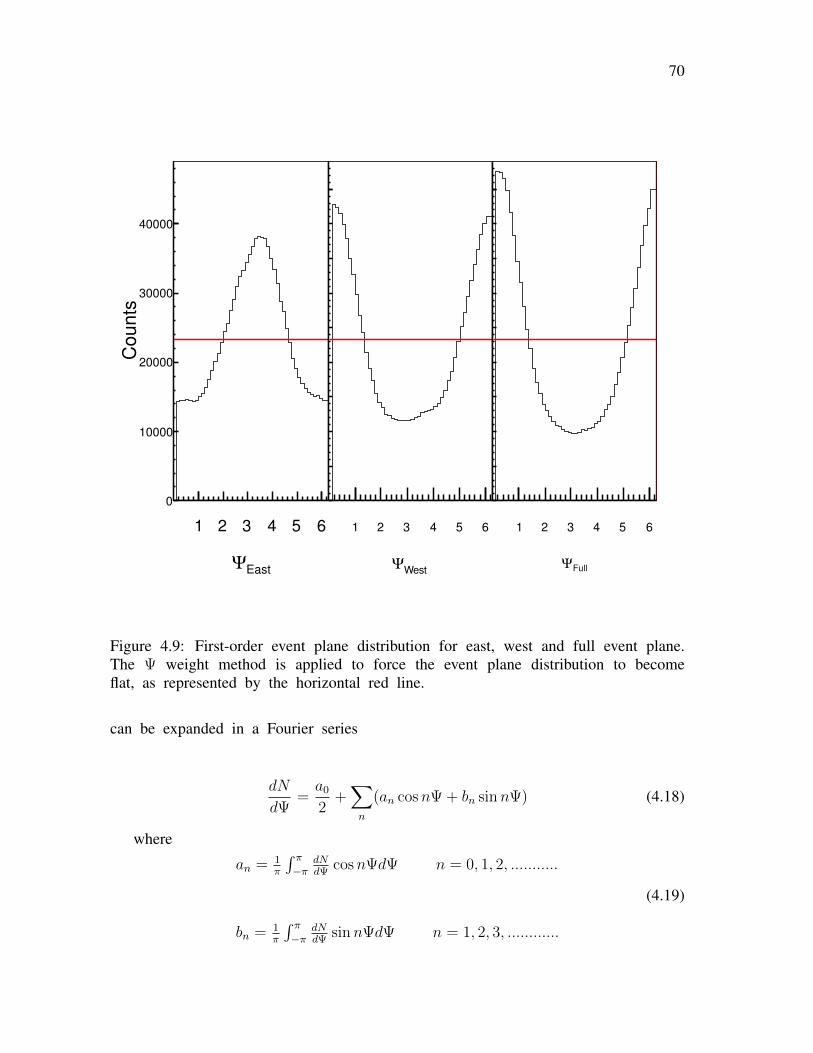
70

EastΨ

1 2 3 4 5 6

Counts

0

10000

20000

30000

40000

WestΨ

1 2 3 4 5 6

0

5000

10000

15000

20000

25000

30000

35000

40000

45000

FullΨ

1 2 3 4 5 6

0

5000

10000

15000

20000

25000

30000

35000

40000

45000

Figure 4.9: First-order event plane distribution for east, west and full event plane.The Ψ weight method is applied to force the event plane distribution to becomeflat, as represented by the horizontal red line.

can be expanded in a Fourier series

dN

dΨ=a0

2+∑n

(an cosnΨ + bn sinnΨ) (4.18)

where

an = 1π

∫ π−π

dNdΨ

cosnΨdΨ n = 0, 1, 2, ...........

bn = 1π

∫ π−π

dNdΨ

sinnΨdΨ n = 1, 2, 3, ............

(4.19)

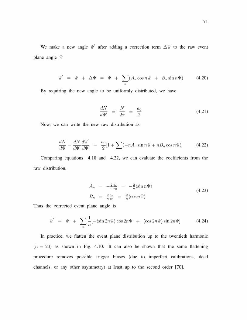
71

We make a new angle Ψ′ after adding a correction term ∆Ψ to the raw event

plane angle Ψ

Ψ′

= Ψ + ∆Ψ = Ψ +∑n

(An cosnΨ + Bn sinnΨ) (4.20)

By requiring the new angle to be uniformly distributed, we have

dN

dΨ′=

N

2π=

a0

2(4.21)

Now, we can write the new raw distribution as

dN

dΨ=dN

dΨ′dΨ

′

dΨ=

a0

2[1 +

∑(−nAn sinnΨ + nBn cosnΨ)] (4.22)

Comparing equations 4.18 and 4.22, we can evaluate the coefficients from the

raw distribution,

An = − 2nbna0

= − 2n〈sinnΨ〉

Bn = 2nana0

= 2n〈cosnΨ〉

(4.23)

Thus the corrected event plane angle is

Ψ′

= Ψ +∑n

1

n[−〈sin 2nΨ〉 cos 2nΨ + 〈cos 2nΨ〉 sin 2nΨ] (4.24)

In practice, we flatten the event plane distribution up to the twentieth harmonic

(n = 20) as shown in Fig. 4.10. It can also be shown that the same flattening

procedure removes possible trigger biases (due to imperfect calibrations, dead

channels, or any other asymmetry) at least up to the second order [70].

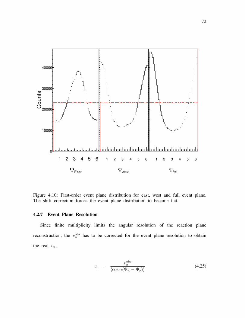
72

EastΨ

1 2 3 4 5 6

Counts

0

10000

20000

30000

40000

WestΨ

1 2 3 4 5 6

0

5000

10000

15000

20000

25000

30000

35000

40000

45000

FullΨ

1 2 3 4 5 6

0

5000

10000

15000

20000

25000

30000

35000

40000

45000

Figure 4.10: First-order event plane distribution for east, west and full event plane.The shift correction forces the event plane distribution to became flat.

4.2.7 Event Plane Resolution

Since finite multiplicity limits the angular resolution of the reaction plane

reconstruction, the vobsn has to be corrected for the event plane resolution to obtain

the real vn,

vn =vobsn

〈cosn(Ψn −Ψr)〉(4.25)

73

Figure 4.11: The event plane resolution for the nth (n = km) harmonic of a particledistribution with respect to the mth harmonic plane, as a function of χm = vm/σ.This plot is from Ref. [14].

where angle brackets denote an average over a large event sample. The event

plane resolution is the denominator of the above equation. For the case of the

1st-order event plane from the BBC, m = 1 and the event plane resolution for

the k-th harmonic calculation reduces to 〈cos k(Ψ1 − Ψr)〉. The BBC event plane

obtained from the detector on one side of the collision (east or west) is called a

sub-event plane. We have two independent sub-event planes from the two BBCs.

The correlation between these two event plane angles can be expressed as

〈cos k(Ψeast −Ψwest)〉 = 〈cos k(Ψeast −Ψr)〉〈cos k(Ψwest −Ψr)〉 (4.26)

If we assume that the two sub-event planes have the same resolution, then the

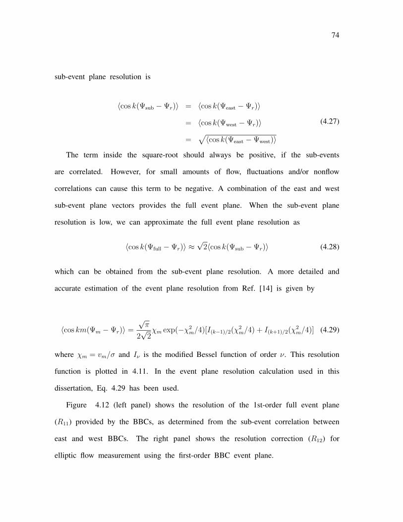
74

sub-event plane resolution is

〈cos k(Ψsub −Ψr)〉 = 〈cos k(Ψeast −Ψr)〉

= 〈cos k(Ψwest −Ψr)〉

=√〈cos k(Ψeast −Ψwest)〉

(4.27)

The term inside the square-root should always be positive, if the sub-events

are correlated. However, for small amounts of flow, fluctuations and/or nonflow

correlations can cause this term to be negative. A combination of the east and west

sub-event plane vectors provides the full event plane. When the sub-event plane

resolution is low, we can approximate the full event plane resolution as

〈cos k(Ψfull −Ψr)〉 ≈√

2〈cos k(Ψsub −Ψr)〉 (4.28)

which can be obtained from the sub-event plane resolution. A more detailed and

accurate estimation of the event plane resolution from Ref. [14] is given by

〈cos km(Ψm −Ψr)〉 =

√π

2√

2χm exp(−χ2

m/4)[I(k−1)/2(χ2m/4) + I(k+1)/2(χ2

m/4)] (4.29)

where χm = vm/σ and Iν is the modified Bessel function of order ν. This resolution

function is plotted in 4.11. In the event plane resolution calculation used in this

dissertation, Eq. 4.29 has been used.

Figure 4.12 (left panel) shows the resolution of the 1st-order full event plane

(R11) provided by the BBCs, as determined from the sub-event correlation between

east and west BBCs. The right panel shows the resolution correction (R12) for

elliptic flow measurement using the first-order BBC event plane.

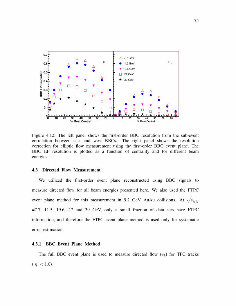
75

% Most Central

0 10 20 30 40 50 60 70

BB

C E

P R

eso

luti

on

0

0.1

0.2

0.3

0.4

0.5

0.6

0.7

11R

% Most Central

0 10 20 30 40 50 60 700

0.1

0.2

0.3

0.4

0.5

0.6

0.7

12R

7.7 GeV

11.5 GeV

19.6 GeV

27 GeV

39 GeV

Figure 4.12: The left panel shows the first-order BBC resolution from the sub-eventcorrelation between east and west BBCs. The right panel shows the resolutioncorrection for elliptic flow measurement using the first-order BBC event plane. TheBBC EP resolution is plotted as a function of centrality and for different beamenergies.

4.3 Directed Flow Measurement

We utilized the first-order event plane reconstructed using BBC signals to

measure directed flow for all beam energies presented here. We also used the FTPC

event plane method for this measurement in 9.2 GeV AuAu collisions. At√sNN

=7.7, 11.5, 19.6, 27 and 39 GeV, only a small fraction of data sets have FTPC

information, and therefore the FTPC event plane method is used only for systematic

error estimation.

4.3.1 BBC Event Plane Method

The full BBC event plane is used to measure directed flow (v1) for TPC tracks

(|η| < 1.0)

76

v1{BBC} =〈cos(φ−ΨBBC)〉

C√〈cos(ΨBBCη−

−ΨBBCη+)〉

(4.30)

The denominator in Eq. (4.30) represents the full BBC event plane resolution.

We use subevents reconstructed in opposite pseudorapidity regions for FTPC tracks

(2.5 < |η| < 4.2),

v1{BBCη−} =〈cos(φ−ΨBBCη+

)〉√〈cos(ΨBBCη−

−ΨBBCη+)〉

(4.31)

v1{BBCη+} =〈cos(φ−ΨBBCη−

)〉√〈cos(ΨBBCη−

−ΨBBCη+)〉

(4.32)

This method effectively avoids self-correlation because of partial overlap between

FTPC and BBC coverage.

4.3.2 FTPC Event Plane Method

For the TPC coverage (|η| < 1) we use the full FTPC event plane,

v1{FTPC} =〈cos(φ−ΨFTPC)〉

C√〈cos(ΨFTPCη−

−ΨFTPCη+)〉

(4.33)

The denominator in Eq. (4.50) represents the full FTPC event plane resolution.

We use subevents reconstructed in opposite pseudorapidity regions for FTPC tracks

(2.5 < |η| < 4.2),

v1{FTPCη−} =〈cos(φ−ΨFTPCη+

)〉√〈cos(ΨFTPCη−

−ΨFTPCη+)〉

(4.34)

v1{FTPCη+} =〈cos(φ−ΨFTPCη−

)〉√〈cos(ΨFTPCη−

−ΨFTPCη+)〉

(4.35)

This method avoids self-correlation.

77

4.4 Elliptic Flow Measurement

The first order event plane reconstructed using BBC signals is used to measure

elliptic flow for AuAu collisions at√sNN = 7.7, 11.5, 19.6, 27 and 39 GeV. The

BBC event plane resolution for v2 measurement for CuCu collision at 22.4 GeV

data set is very poor [74]. Therefore, the second-order event plane reconstructed

from the TPC is used to measure v2 for this data set.

4.4.1 BBC Event Plane Method

In this method, the elliptic flow v2 is obtained correlating the particles with the

first order BBC event plane.

v2{BBC} =〈cos 2(φ−ΨBBC)〉

R12

(4.36)

where R12 is the event plane resolution for n = 2 (m = 1, k = 2), when v2 is

measured with respect to the first-order event plane.

4.4.2 TPC Event Plane Method

In this method, v2 is measured with respect to the second-order event plane

reconstructed using the TPC tracks. In event plane calculations, tracks have a

weighting factor w = pT in units of GeV/c for pT < 2 GeV/c, and w = 2 GeV/c

for pT ≥ GeV/c. The η sub-event method is used where one defines the flow

vector for each particle based on particles measured in the opposite hemisphere in

pseudorapidity:

v2{EtaSubs} =〈cos 2(φ± −Ψ2,η∓)〉√〈cos 2(Ψ2,η+ −Ψ2,η−)〉

(4.37)

Here v2{EtaSubs} denotes the results of the η sub-event method, and Ψ2,η+(Ψ2,η+)

78

is the second harmonic event plane angle determined by particles with posi-

tive/negative pseudorapidity. A small additional η gap is used between nega-

tive/positive η sub-events to suppress non-flow effects.

4.4.3 The Cumulant Method

The Q-cumulants method [75], also sometimes called the direct cumulant method,

calculates cumulants without using nested loops over tracks. The cumulants are

expressed in terms of the moments of the magnitude of the corresponding flow

vector,

Qn ≡M∑i=1

einφi (4.38)

The single-event average two- and four-particle azimuthal correlations can be then

formulated as [75]:

〈2〉 =|Qn|2 −MM(M − 1)

(4.39)

〈4〉 =|Qn|4 + |Q2n|2 − 2< [Q2nQ

∗nQ∗n]

M(M − 1)(M − 2)(M − 3)

− 22(M − 2)|Qn|2 −M(M − 3)

M(M − 1)(M − 2)(M − 3)

(4.40)

The average over all events can be performed as:

〈〈2〉〉 ≡ 〈ein(φ1−φ2)〉

=

∑event

(W〈2〉

)i〈2〉i∑

event

(W〈2〉

)i

(4.41)

〈〈4〉〉 ≡ 〈ein(φ1+φ2−φ3−φ4)〉

=

∑events

(W〈4〉

)i〈4〉i∑

events

(W〈4〉

)i

(4.42)

while the weights are the number of two- and four-particle combinations:

W〈2〉 ≡M(M − 1), (4.43)

79

W〈4〉 ≡M(M − 1)(M − 2)(M − 3). (4.44)

Choosing the multiplicity weights above can make the final multi-particle azimuthal

correlations free of multiplicity fluctuations [76]. However, one can also use unit

weights treating events with different multiplicity equally. The two- and four-particle

cumulants without detector bias can be formulated as:

cn{2} = 〈〈2〉〉 (4.45)

cn{4} = 〈〈4〉〉 − 2〈〈2〉〉2 (4.46)

The integrated flow (e.g. integrated over pT and η) can be estimated both from

two- and four-particle cumulants:

vn{2} =√cn{2} (4.47)

vn{4} = 4√−cn{4} (4.48)

In this method, the higher order multi-particle correlation formalism removes the

contribution of non-flow correlations from lower order correlations [75, 76].

4.5 Triangular Flow Measurement

There are various methods to obtain triangular flow results. Two-particle cor-

relations which are sensitive to non-flow correlations and multiparticle correlations

which are less sensitive to the non-flow correlations along with event plane methods

have been extensively used in elliptic flow measurements for past couple of decades.

These methods used in elliptic flow analysis can be extended to measure triangular

flow. The event plane method, and the two-particle cumulant method, which are

used in v3 analysis for this dissertation, are discussed below.

80

4.5.1 Event Plane Methods

In the standard event plane method [14] for v3, we reconstruct a third-harmonic

event plane from TPC tracks and also from FTPC tracks. In event plane calculations,

tracks have a weighting factor w = pT in units of GeV/c for pT < 2 GeV/c, and

w = 2 GeV/c for pT ≥ 2 GeV/c. Although the STAR detector has good azimuthal

symmetry, small acceptance effects in the calculation of the event plane azimuth

were removed by the method of shifting [73]. When using the TPC event plane,

we used the η sub-event method with an additional η gap of ± 0.05.

v3{EtaSubs} =〈cos 3(φ± −Ψ3,η∓)〉√〈cos 3(Ψ3,η+ −Ψ3,η−)〉

(4.49)

This avoids self-correlations because the particles and the event plane are in

opposite hemispheres. When using the FTPCs, we used the full event plane from

both FTPCs [14].

v3{FTPC} =〈cos 3(φ−Ψ3FTPC)〉

C√〈cos 3(Ψ3,FTPCη+ −Ψ3,FTPCη−)〉

(4.50)

This introduced a large η gap between the particles and the event plane. Since there

is no overlap between the coverage of the TPC and FTPCs, there is no possibility

of self-correlation when using the FTPC event plane.

4.5.2 Two-Particle Correlation Method

I study 〈cos 3(φj − φi)〉i 6=j vs ∆η between two particles with indices i and j to

understand the ∆η dependence of the triangular flow signal and to distinguish among

different sources of non-flow correlations. This distribution of 〈cos 3(φj − φi)〉i 6=j

vs. ∆η can be well described by wide and narrow Gaussian peaks as shown

in Fig. 4.13 for two centrality intervals. The narrow Gaussian is identified with

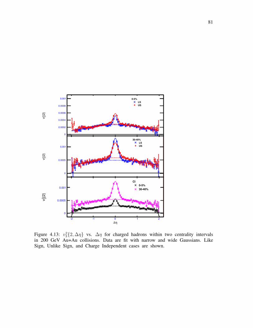
81

2 1 0 1 2

{2}

2 3v

0

0.0002

0.0004

0.0006

0.0008

0.001 05%

LS

US

2 1 0 1 2

{2}

2 3v

0

0.0005

0.001

3040%

LS

US

η∆

2 1 0 1 2

{2}

2 3v

0

0.0005

0.001

CI

05%

3040%

Figure 4.13: v23{2,∆η} vs. ∆η for charged hadrons within two centrality intervals

in 200 GeV Au+Au collisions. Data are fit with narrow and wide Gaussians. LikeSign, Unlike Sign, and Charge Independent cases are shown.

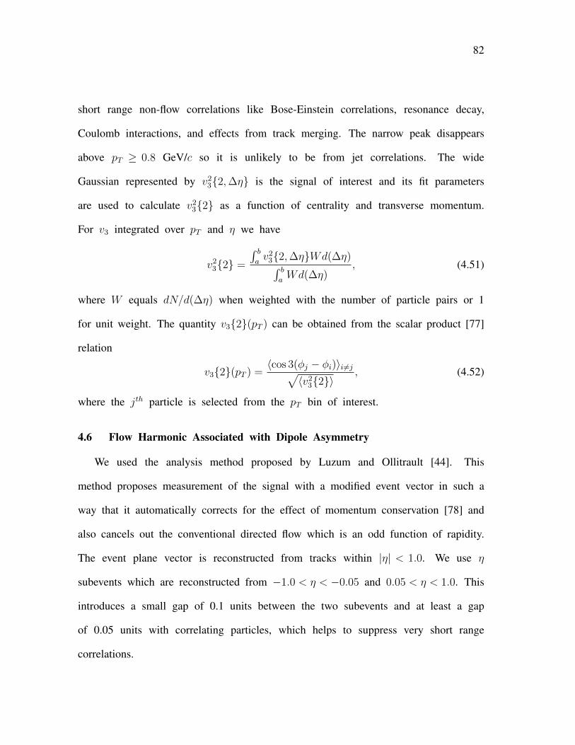
82

short range non-flow correlations like Bose-Einstein correlations, resonance decay,

Coulomb interactions, and effects from track merging. The narrow peak disappears

above pT ≥ 0.8 GeV/c so it is unlikely to be from jet correlations. The wide

Gaussian represented by v23{2,∆η} is the signal of interest and its fit parameters

are used to calculate v23{2} as a function of centrality and transverse momentum.

For v3 integrated over pT and η we have

v23{2} =

∫ bav2

3{2,∆η}Wd(∆η)∫ baWd(∆η)

, (4.51)

where W equals dN/d(∆η) when weighted with the number of particle pairs or 1

for unit weight. The quantity v3{2}(pT ) can be obtained from the scalar product [77]

relation

v3{2}(pT ) =〈cos 3(φj − φi)〉i 6=j√

〈v23{2}〉

, (4.52)

where the jth particle is selected from the pT bin of interest.

4.6 Flow Harmonic Associated with Dipole Asymmetry

We used the analysis method proposed by Luzum and Ollitrault [44]. This

method proposes measurement of the signal with a modified event vector in such a

way that it automatically corrects for the effect of momentum conservation [78] and

also cancels out the conventional directed flow which is an odd function of rapidity.

The event plane vector is reconstructed from tracks within |η| < 1.0. We use η

subevents which are reconstructed from −1.0 < η < −0.05 and 0.05 < η < 1.0. This

introduces a small gap of 0.1 units between the two subevents and at least a gap

of 0.05 units with correlating particles, which helps to suppress very short range

correlations.

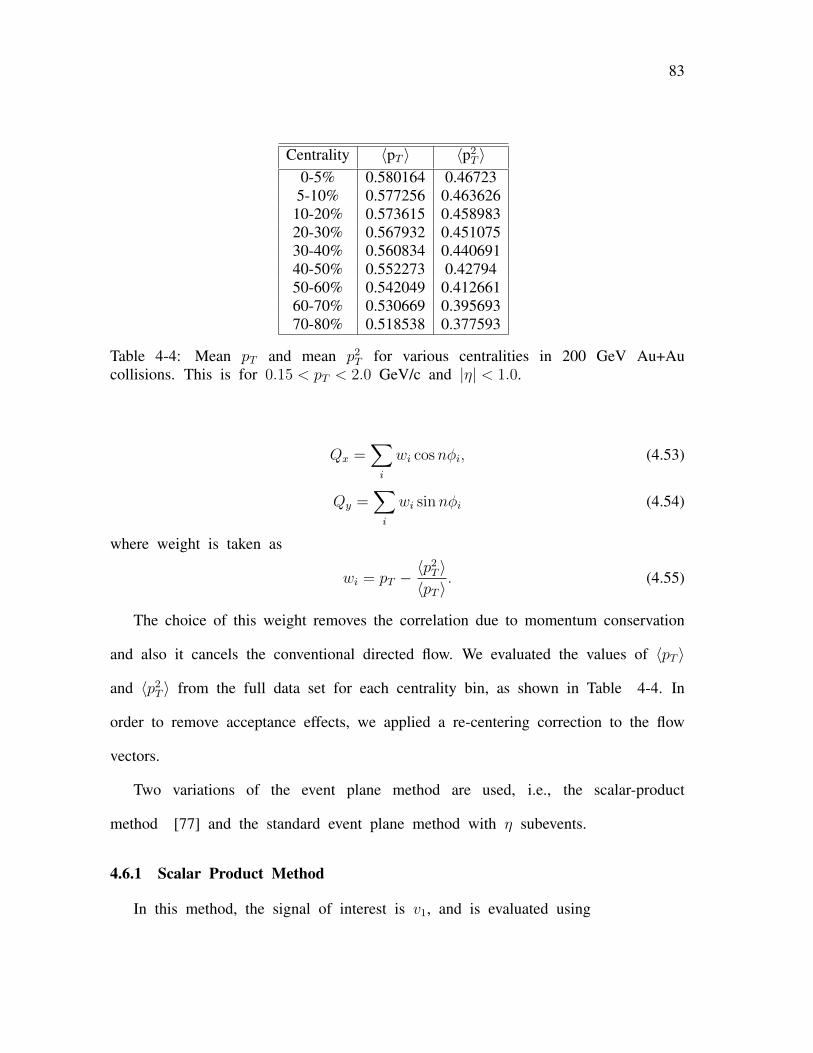
83

Centrality 〈pT 〉〈p2T 〉

0-5% 0.580164 0.467235-10% 0.577256 0.463626

10-20% 0.573615 0.45898320-30% 0.567932 0.45107530-40% 0.560834 0.44069140-50% 0.552273 0.4279450-60% 0.542049 0.41266160-70% 0.530669 0.39569370-80% 0.518538 0.377593

Table 4-4: Mean pT and mean p2T for various centralities in 200 GeV Au+Au

collisions. This is for 0.15 < pT < 2.0 GeV/c and |η| < 1.0.

Qx =∑i

wi cosnφi, (4.53)

Qy =∑i

wi sinnφi (4.54)

where weight is taken as

wi = pT −〈p2T 〉〈pT 〉

. (4.55)

The choice of this weight removes the correlation due to momentum conservation

and also it cancels the conventional directed flow. We evaluated the values of 〈pT 〉

and 〈p2T 〉 from the full data set for each centrality bin, as shown in Table 4-4. In

order to remove acceptance effects, we applied a re-centering correction to the flow

vectors.

Two variations of the event plane method are used, i.e., the scalar-product

method [77] and the standard event plane method with η subevents.

4.6.1 Scalar Product Method

In this method, the signal of interest is v1, and is evaluated using

84

v1(η > 0) =〈Qa(η < 0).ui)〉√

〈Qa.Qb〉(4.56)

v1(η < 0) =〈Qb(η > 0).ui)〉√

〈Qa.Qb〉(4.57)

where ui = eiφ is the unit vector of a particle. The vectors Qa and Qb are

constructed from the subevents a(η < 0) and b(η > 0).

This subevent method effectively removes the self-correlation.

4.6.2 Event Plane method

In the event plane method, we first evaluate the event plane azimuth Ψ1 from

the event plane vector:

Ψn =

(tan−1 Qy

Qx

)(4.58)

Then

v1{η > 0} =〈cos n[φ−Ψa(η < 0)]〉√

〈 cos[Ψa(η < 0)−Ψb(η > 0)]〉. (4.59)

v1{η < 0} =〈cos n[φ−Ψb(η > 0)]〉√

〈 cos[Ψa(η < 0)−Ψb(η > 0)]〉. (4.60)

Use of the subevent plane method removes the effect from self correlation.

4.7 Systematic Uncertainties

In this section, various possible sources of systematic uncertainties and their

estimation are discussed.

85

4.7.1 Event Plane Determination

The event plane resolution depends on the number of tracks used to reconstruct

the event plane. Therefore changing event and track cuts obviously changes the

event plane resolution. Therefore we can not use these techniques to estimate the

systematic uncertainty. Instead we changed the flattening technique to estimate the

systematic errors in these studies. We used the shifting method to make the event

plane flat as the default method. The difference in event plane resolution between

the shift method and ψ weight method is our estimate of the systematic error

coming from event plane determination. The systematic errors from the flattening

process are less than 1% for all event plane methods.

4.7.2 Detector Acceptance and Efficiency

We estimate systematic errors in measurements coming from detector effects by

changing event and track quality cuts. We vary the vz cut, Nfit points, DCA,

lower and the upper transverse momentum cut. These are the main tests used to

estimate the systematic errors. We also changed PID cuts to estimate the error due

to particle misidentification.

4.7.3 East-West Symmetry

The STAR detector has east-west symmetry. We compared our results for positive

and negative pseudorapidity, positive and negative vz and the absolute difference is

considered to a measure of systematic uncertainty.

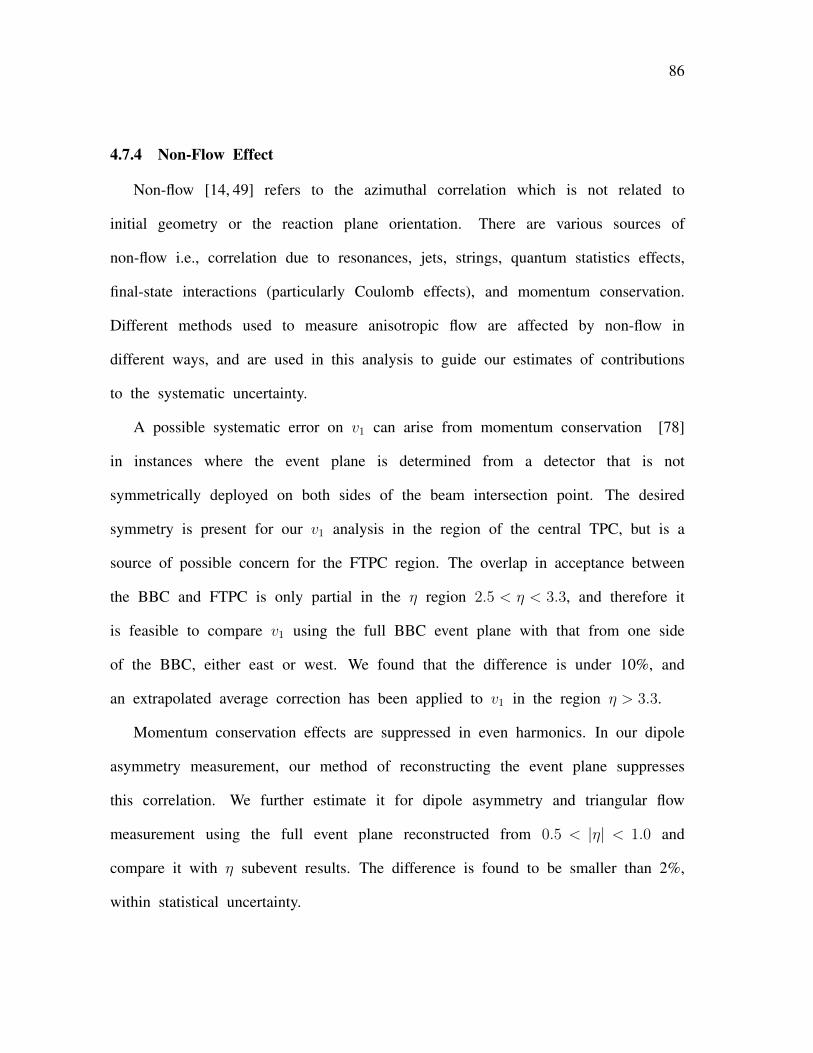
86

4.7.4 Non-Flow Effect

Non-flow [14, 49] refers to the azimuthal correlation which is not related to

initial geometry or the reaction plane orientation. There are various sources of

non-flow i.e., correlation due to resonances, jets, strings, quantum statistics effects,

final-state interactions (particularly Coulomb effects), and momentum conservation.

Different methods used to measure anisotropic flow are affected by non-flow in

different ways, and are used in this analysis to guide our estimates of contributions

to the systematic uncertainty.

A possible systematic error on v1 can arise from momentum conservation [78]

in instances where the event plane is determined from a detector that is not

symmetrically deployed on both sides of the beam intersection point. The desired

symmetry is present for our v1 analysis in the region of the central TPC, but is a

source of possible concern for the FTPC region. The overlap in acceptance between

the BBC and FTPC is only partial in the η region 2.5 < η < 3.3, and therefore it

is feasible to compare v1 using the full BBC event plane with that from one side

of the BBC, either east or west. We found that the difference is under 10%, and

an extrapolated average correction has been applied to v1 in the region η > 3.3.

Momentum conservation effects are suppressed in even harmonics. In our dipole

asymmetry measurement, our method of reconstructing the event plane suppresses

this correlation. We further estimate it for dipole asymmetry and triangular flow

measurement using the full event plane reconstructed from 0.5 < |η| < 1.0 and

compare it with η subevent results. The difference is found to be smaller than 2%,

within statistical uncertainty.

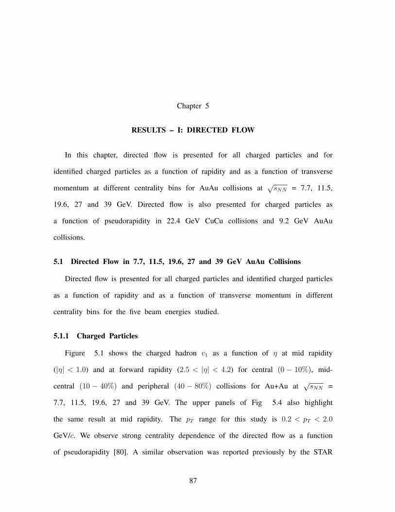
Chapter 5

RESULTS – I: DIRECTED FLOW

In this chapter, directed flow is presented for all charged particles and for

identified charged particles as a function of rapidity and as a function of transverse

momentum at different centrality bins for AuAu collisions at√sNN = 7.7, 11.5,

19.6, 27 and 39 GeV. Directed flow is also presented for charged particles as

a function of pseudorapidity in 22.4 GeV CuCu collisions and 9.2 GeV AuAu

collisions.

5.1 Directed Flow in 7.7, 11.5, 19.6, 27 and 39 GeV AuAu Collisions

Directed flow is presented for all charged particles and identified charged particles

as a function of rapidity and as a function of transverse momentum in different

centrality bins for the five beam energies studied.

5.1.1 Charged Particles

Figure 5.1 shows the charged hadron v1 as a function of η at mid rapidity

(|η| < 1.0) and at forward rapidity (2.5 < |η| < 4.2) for central (0 − 10%), mid-

central (10 − 40%) and peripheral (40 − 80%) collisions for Au+Au at√sNN =

7.7, 11.5, 19.6, 27 and 39 GeV. The upper panels of Fig 5.4 also highlight

the same result at mid rapidity. The pT range for this study is 0.2 < pT < 2.0

GeV/c. We observe strong centrality dependence of the directed flow as a function

of pseudorapidity [80]. A similar observation was reported previously by the STAR

87

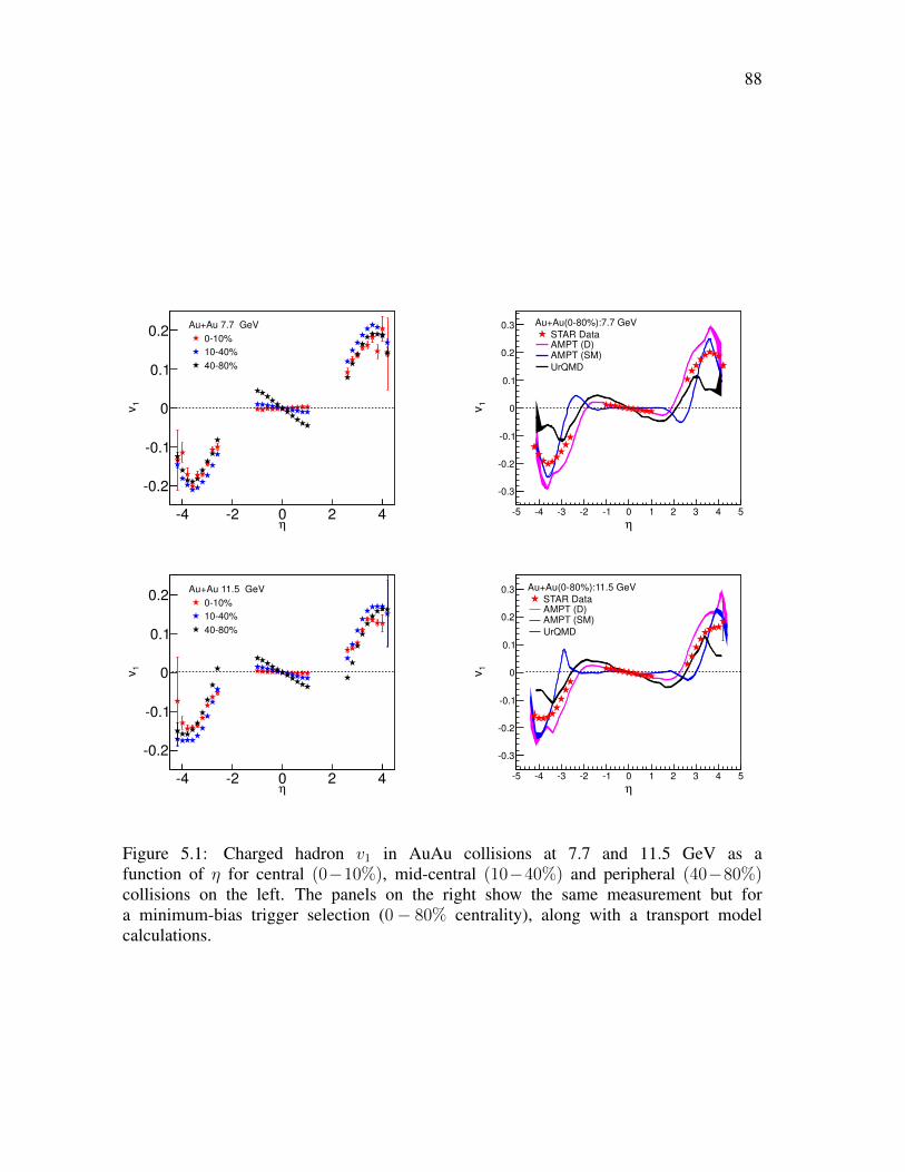
88

η4 2 0 2 4

1v

0.2

0.1

0

0.1

0.2Au+Au 7.7 GeV

010%

1040%

4080%

η

5 4 3 2 1 0 1 2 3 4 5

1v

0.3

0.2

0.1

0

0.1

0.2

0.3 Au+Au(080%):7.7 GeV

STAR Data AMPT (D)AMPT (SM)

UrQMD

η4 2 0 2 4

1v

0.2

0.1

0

0.1

0.2Au+Au 11.5 GeV

010%

1040%

4080%

η

5 4 3 2 1 0 1 2 3 4 5

1v

0.3

0.2

0.1

0

0.1

0.2

0.3 Au+Au(080%):11.5 GeV

STAR Data AMPT (D)AMPT (SM)

UrQMD

Figure 5.1: Charged hadron v1 in AuAu collisions at 7.7 and 11.5 GeV as afunction of η for central (0−10%), mid-central (10−40%) and peripheral (40−80%)collisions on the left. The panels on the right show the same measurement but fora minimum-bias trigger selection (0− 80% centrality), along with a transport modelcalculations.

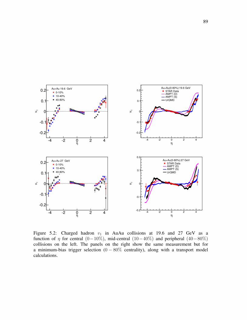
89

η4 2 0 2 4

1v

0.2

0.1

0

0.1

0.2Au+Au 19.6 GeV

010%

1040%

4080%

η

4 2 0 2 4

1v

0.2

0.1

0

0.1

0.2Au+Au(080%):19.6 GeV

STAR Data AMPT (D)AMPT (S)

UrQMD

η4 2 0 2 4

1v

0.2

0.1

0

0.1

0.2Au+Au 27 GeV

010%

1040%

4080%

η

4 2 0 2 4

1v

0.2

0.1

0

0.1

0.2Au+Au(080%):27 GeV


UrQMD

Figure 5.2: Charged hadron v1 in AuAu collisions at 19.6 and 27 GeV as afunction of η for central (0−10%), mid-central (10−40%) and peripheral (40−80%)collisions on the left. The panels on the right show the same measurement but fora minimum-bias trigger selection (0− 80% centrality), along with a transport modelcalculations.

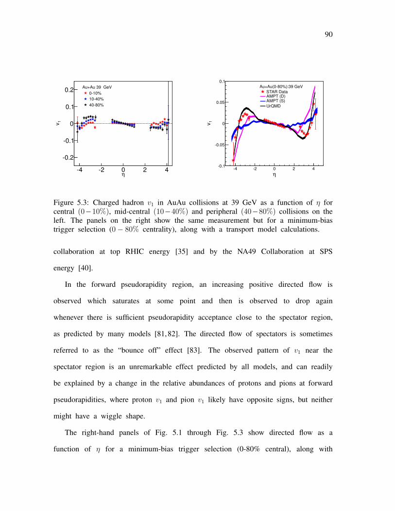
90

η4 2 0 2 4

1v

0.2

0.1

0

0.1

0.2Au+Au 39 GeV

010%

1040%

4080%

η

4 2 0 2 4

1v

0.1

0.05

0

0.05

0.1

Au+Au(080%):39 GeV


UrQMD

Figure 5.3: Charged hadron v1 in AuAu collisions at 39 GeV as a function of η forcentral (0−10%), mid-central (10−40%) and peripheral (40−80%) collisions on theleft. The panels on the right show the same measurement but for a minimum-biastrigger selection (0− 80% centrality), along with a transport model calculations.

collaboration at top RHIC energy [35] and by the NA49 Collaboration at SPS

energy [40].

In the forward pseudorapidity region, an increasing positive directed flow is

observed which saturates at some point and then is observed to drop again

whenever there is sufficient pseudorapidity acceptance close to the spectator region,

as predicted by many models [81,82]. The directed flow of spectators is sometimes

referred to as the “bounce off” effect [83]. The observed pattern of v1 near the

spectator region is an unremarkable effect predicted by all models, and can readily

be explained by a change in the relative abundances of protons and pions at forward

pseudorapidities, where proton v1 and pion v1 likely have opposite signs, but neither

might have a wiggle shape.

The right-hand panels of Fig. 5.1 through Fig. 5.3 show directed flow as a

function of η for a minimum-bias trigger selection (0-80% central), along with

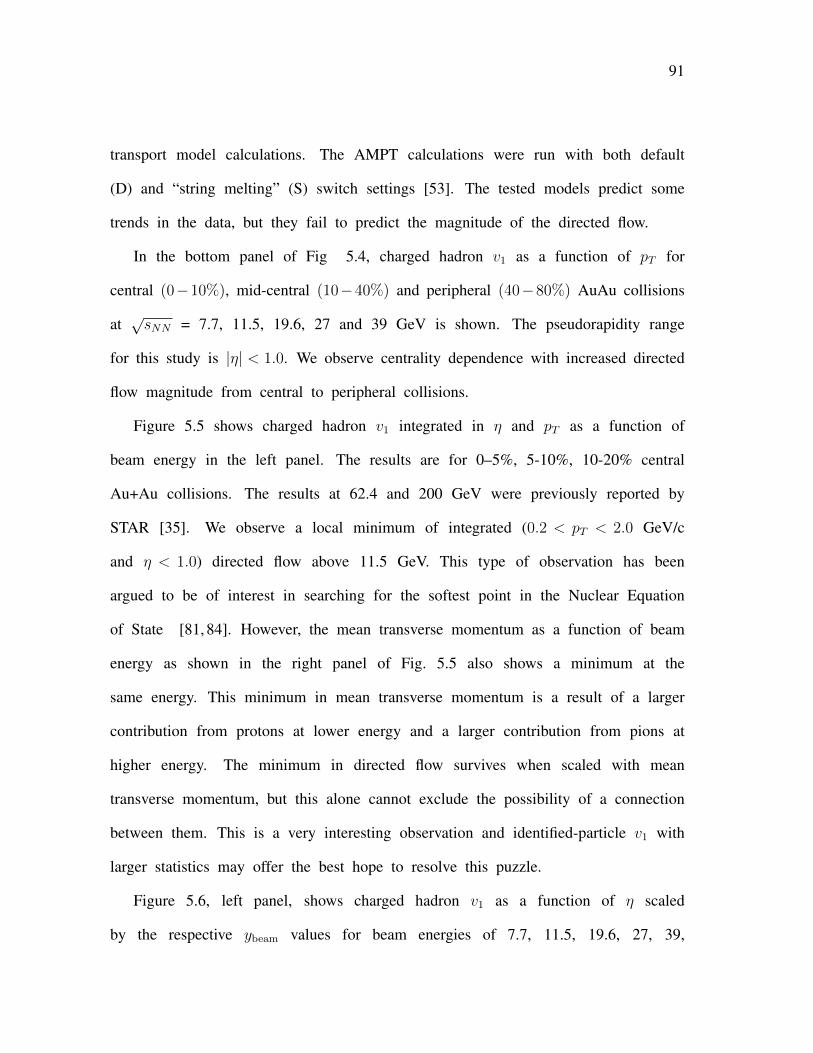
91

transport model calculations. The AMPT calculations were run with both default

(D) and “string melting” (S) switch settings [53]. The tested models predict some

trends in the data, but they fail to predict the magnitude of the directed flow.

In the bottom panel of Fig 5.4, charged hadron v1 as a function of pT for

central (0−10%), mid-central (10−40%) and peripheral (40−80%) AuAu collisions

at√sNN = 7.7, 11.5, 19.6, 27 and 39 GeV is shown. The pseudorapidity range

for this study is |η| < 1.0. We observe centrality dependence with increased directed

flow magnitude from central to peripheral collisions.

Figure 5.5 shows charged hadron v1 integrated in η and pT as a function of

beam energy in the left panel. The results are for 0–5%, 5-10%, 10-20% central

Au+Au collisions. The results at 62.4 and 200 GeV were previously reported by

STAR [35]. We observe a local minimum of integrated (0.2 < pT < 2.0 GeV/c

and η < 1.0) directed flow above 11.5 GeV. This type of observation has been

argued to be of interest in searching for the softest point in the Nuclear Equation

of State [81, 84]. However, the mean transverse momentum as a function of beam

energy as shown in the right panel of Fig. 5.5 also shows a minimum at the

same energy. This minimum in mean transverse momentum is a result of a larger

contribution from protons at lower energy and a larger contribution from pions at

higher energy. The minimum in directed flow survives when scaled with mean

transverse momentum, but this alone cannot exclude the possibility of a connection

between them. This is a very interesting observation and identified-particle v1 with

larger statistics may offer the best hope to resolve this puzzle.

Figure 5.6, left panel, shows charged hadron v1 as a function of η scaled

by the respective ybeam values for beam energies of 7.7, 11.5, 19.6, 27, 39,

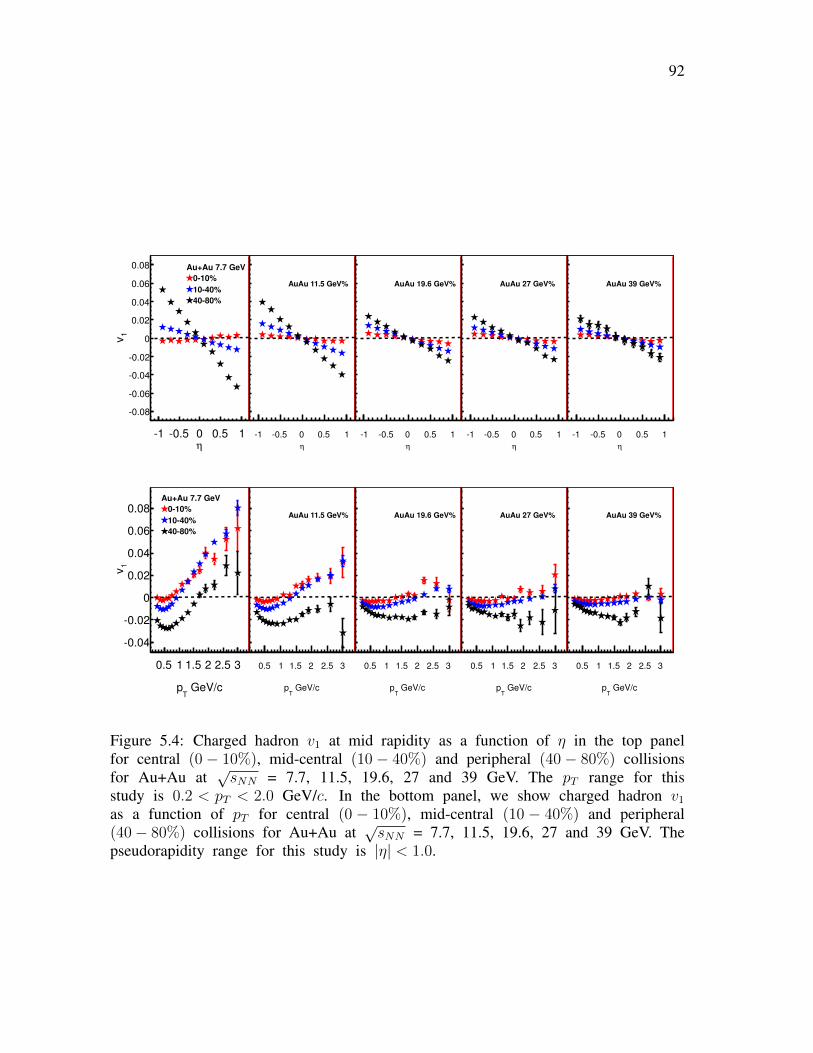
92

η

1 0.5 0 0.5 1

1v

0.08

0.06

0.04

0.02

0

0.02

0.04

0.06

0.08 Au+Au 7.7 GeV

010%

1040%

4080%

η

1 0.5 0 0.5 1

0.08

0.06

0.04

0.02

0

0.02

0.04

0.06

0.08

AuAu 11.5 GeV%

η

1 0.5 0 0.5 1

0.08

0.06

0.04

0.02

0

0.02

0.04

0.06

0.08

AuAu 19.6 GeV%

η

1 0.5 0 0.5 1

0.08

0.06

0.04

0.02

0

0.02

0.04

0.06

0.08

AuAu 27 GeV%

η

1 0.5 0 0.5 1

0.08

0.06

0.04

0.02

0

0.02

0.04

0.06

0.08

AuAu 39 GeV%

GeV/cT

p

0.5 1 1.5 2 2.5 3

1v

0.04

0.02

0

0.02

0.04

0.06

0.08Au+Au 7.7 GeV

010%

1040%

4080%

GeV/cT

p

0.5 1 1.5 2 2.5 3

0.04

0.02

0

0.02

0.04

0.06

0.08AuAu 11.5 GeV%

GeV/cT

p

0.5 1 1.5 2 2.5 3

0.04

0.02

0

0.02

0.04

0.06

0.08AuAu 19.6 GeV%

GeV/cT

p

0.5 1 1.5 2 2.5 3

0.04

0.02

0

0.02

0.04

0.06

0.08AuAu 27 GeV%

GeV/cT

p

0.5 1 1.5 2 2.5 3

0.04

0.02

0

0.02

0.04

0.06

0.08AuAu 39 GeV%

Figure 5.4: Charged hadron v1 at mid rapidity as a function of η in the top panelfor central (0− 10%), mid-central (10− 40%) and peripheral (40− 80%) collisionsfor Au+Au at

√sNN = 7.7, 11.5, 19.6, 27 and 39 GeV. The pT range for this

study is 0.2 < pT < 2.0 GeV/c. In the bottom panel, we show charged hadron v1

as a function of pT for central (0 − 10%), mid-central (10 − 40%) and peripheral(40− 80%) collisions for Au+Au at

√sNN = 7.7, 11.5, 19.6, 27 and 39 GeV. The

pseudorapidity range for this study is |η| < 1.0.

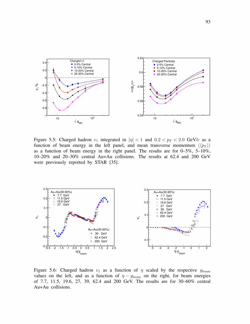
93

NN s√10

210

% 1v

1

0.8

0.6

0.4

0.2

0

0.2

0.4Charged v1

05% Central510% Central1020% Central2030% Central

NN s√10

210

>>

T<

<p

0.54

0.56

0.58

0.6

0.62Charged Particles

05% Central510% Central1020% Central2030% Central

Figure 5.5: Charged hadron v1 integrated in |η| < 1 and 0.2 < pT < 2.0 GeV/c as afunction of beam energy in the left panel, and mean transverse momentum 〈〈pT 〉〉as a function of beam energy in the right panel. The results are for 0–5%, 5–10%,10–20% and 20–30% central Au+Au collisions. The results at 62.4 and 200 GeVwere previously reported by STAR [35].

beam/yη

2.5 2 1.5 1 0.5 0 0.5 1 1.5 2 2.5

1v

0.3

0.2

0.1

0

0.1

0.2

0.3

Au+Au(3060%)

39 GeV

62.4 GeV

200 GeV

Au+Au(3060%)7.7 GeV11.5 GeV19.6 GeV27 GeV

beamyη

5 4 3 2 1 0 1 2

1v

0.1

0

0.1

0.2

0.3Au+Au(3060%)

7.7 GeV11.5 GeV19.6 GeV27 GeV39 GeV62.4 GeV200 GeV

Figure 5.6: Charged hadron v1 as a function of η scaled by the respective ybeam

values on the left, and as a function of η − ybeam on the right, for beam energiesof 7.7, 11.5, 19.6, 27, 39, 62.4 and 200 GeV. The results are for 30–60% centralAu+Au collisions.

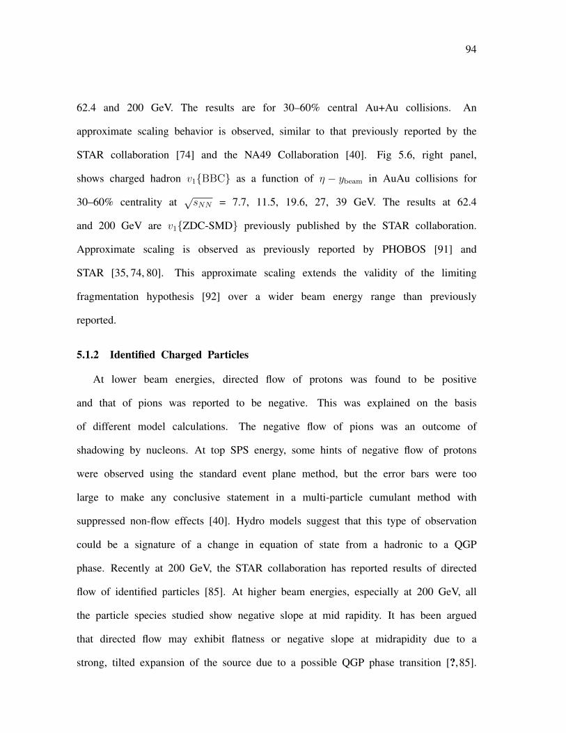
94

62.4 and 200 GeV. The results are for 30–60% central Au+Au collisions. An

approximate scaling behavior is observed, similar to that previously reported by the

STAR collaboration [74] and the NA49 Collaboration [40]. Fig 5.6, right panel,

shows charged hadron v1{BBC} as a function of η − ybeam in AuAu collisions for

30–60% centrality at√sNN = 7.7, 11.5, 19.6, 27, 39 GeV. The results at 62.4

and 200 GeV are v1{ZDC-SMD} previously published by the STAR collaboration.

Approximate scaling is observed as previously reported by PHOBOS [91] and

STAR [35, 74, 80]. This approximate scaling extends the validity of the limiting

fragmentation hypothesis [92] over a wider beam energy range than previously

reported.

5.1.2 Identified Charged Particles

At lower beam energies, directed flow of protons was found to be positive

and that of pions was reported to be negative. This was explained on the basis

of different model calculations. The negative flow of pions was an outcome of

shadowing by nucleons. At top SPS energy, some hints of negative flow of protons

were observed using the standard event plane method, but the error bars were too

large to make any conclusive statement in a multi-particle cumulant method with

suppressed non-flow effects [40]. Hydro models suggest that this type of observation

could be a signature of a change in equation of state from a hadronic to a QGP

phase. Recently at 200 GeV, the STAR collaboration has reported results of directed

flow of identified particles [85]. At higher beam energies, especially at 200 GeV, all

the particle species studied show negative slope at mid rapidity. It has been argued

that directed flow may exhibit flatness or negative slope at midrapidity due to a

strong, tilted expansion of the source due to a possible QGP phase transition [?,85].

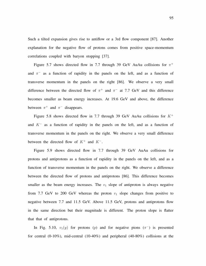
95

Such a tilted expansion gives rise to antiflow or a 3rd flow component [87]. Another

explanation for the negative flow of protons comes from positive space-momentum

correlations coupled with baryon stopping [37].

Figure 5.7 shows directed flow in 7.7 through 39 GeV AuAu collisions for π+

and π− as a function of rapidity in the panels on the left, and as a function of

transverse momentum in the panels on the right [86]. We observe a very small

difference between the directed flow of π+ and π− at 7.7 GeV and this difference

becomes smaller as beam energy increases. At 19.6 GeV and above, the difference

between π+ and π− disappears.

Figure 5.8 shows directed flow in 7.7 through 39 GeV AuAu collisions for K+

and K− as a function of rapidity in the panels on the left, and as a function of

transverse momentum in the panels on the right. We observe a very small difference

between the directed flow of K+ and K−.

Figure 5.9 shows directed flow in 7.7 through 39 GeV AuAu collisions for

protons and antiprotons as a function of rapidity in the panels on the left, and as a

function of transverse momentum in the panels on the right. We observe a difference

between the directed flow of protons and antiprotons [86]. This difference becomes

smaller as the beam energy increases. The v1 slope of antiproton is always negative

from 7.7 GeV to 200 GeV whereas the proton v1 slope changes from positive to

negative between 7.7 and 11.5 GeV. Above 11.5 GeV, protons and antiprotons flow

in the same direction but their magnitude is different. The proton slope is flatter

that that of antiprotons.

In Fig. 5.10, v1(y) for protons (p) and for negative pions (π−) is presented

for central (0-10%), mid-central (10-40%) and peripheral (40-80%) collisions at the

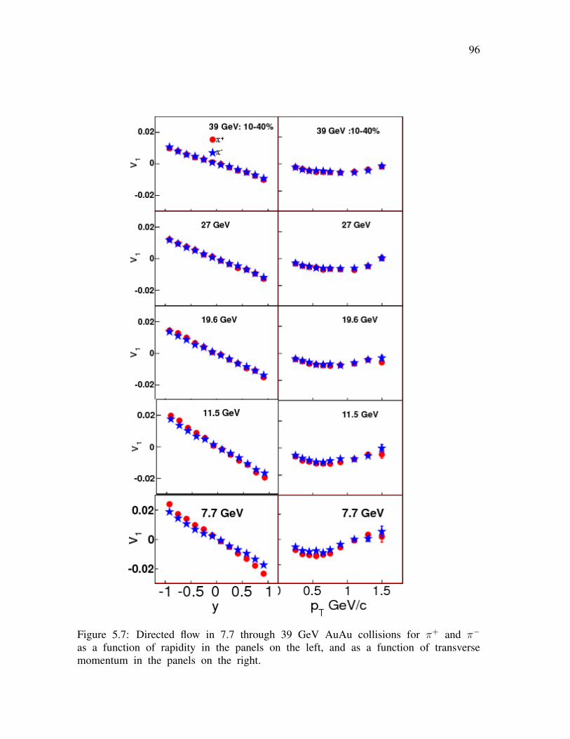
96

Figure 5.7: Directed flow in 7.7 through 39 GeV AuAu collisions for π+ and π−

as a function of rapidity in the panels on the left, and as a function of transversemomentum in the panels on the right.

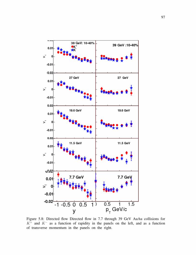
97

Figure 5.8: Directed flow Directed flow in 7.7 through 39 GeV AuAu collisions forK+ and K− as a function of rapidity in the panels on the left, and as a functionof transverse momentum in the panels on the right.

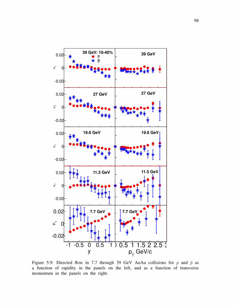
98

1 0.5 0 0.5 1

1v

0.02

0

0.0239 GeV: 1040%

pp

1 0.5 0 0.5 1

1v

0.02

0

0.02 27 GeV

1 0.5 0 0.5 1

1v

0.02

0

0.02 19.6 GeV

1 0.5 0 0.5 1

1v

0.02

0

0.02 11.5 GeV

y1 0.5 0 0.5 1

1v

0.02

0

0.02 7.7 GeV

0 0.5 1 1.5 2 2.5 3

0.02

0

0.0239 GeV

0 0.5 1 1.5 2 2.5 3

0.02

0

0.0227 GeV

0 0.5 1 1.5 2 2.5 3

0.02

0

0.0219.6 GeV

0 0.5 1 1.5 2 2.5 3

0.02

0

0.0211.5 GeV

GeV/c T

p0 0.5 1 1.5 2 2.5 3

0.02

0

0.027.7 GeV

Figure 5.9: Directed flow in 7.7 through 39 GeV AuAu collisions for p and p asa function of rapidity in the panels on the left, and as a function of transversemomentum in the panels on the right.

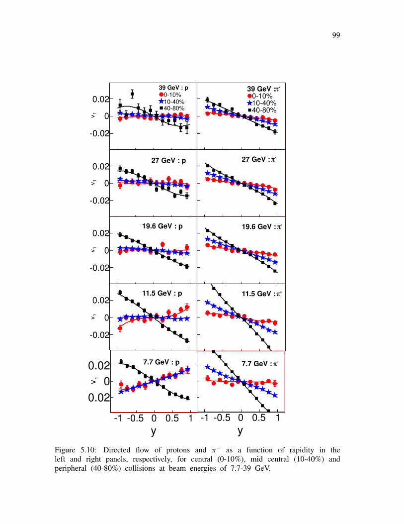
99

1 0.5 0 0.5 1

1v

0.02

0

0.02

39 GeV : p010%

1040%4080%

1 0.5 0 0.5 1

1v

0.02

0

0.0227 GeV : p

1 0.5 0 0.5 1

1v

0.02

0

0.0219.6 GeV : p

1 0.5 0 0.5 1

1v

0.02

0

0.0211.5 GeV : p

y1 0.5 0 0.5 1

1v

0.02

0

0.02 7.7 GeV : p

1 0.5 0 0.5 1

0.02

0

0.02

π39 GeV :

010%1040%4080%

1 0.5 0 0.5 1

0.02

0

0.02

π27 GeV :

1 0.5 0 0.5 1

0.02

0

0.02

π19.6 GeV :

1 0.5 0 0.5 1

0.02

0

0.02

π11.5 GeV :

y1 0.5 0 0.5 1

0.02

0

0.02

π7.7 GeV :

Figure 5.10: Directed flow of protons and π− as a function of rapidity in theleft and right panels, respectively, for central (0-10%), mid central (10-40%) andperipheral (40-80%) collisions at beam energies of 7.7-39 GeV.

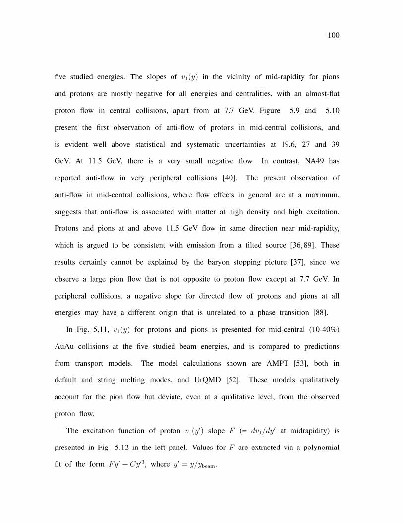
100

five studied energies. The slopes of v1(y) in the vicinity of mid-rapidity for pions

and protons are mostly negative for all energies and centralities, with an almost-flat

proton flow in central collisions, apart from at 7.7 GeV. Figure 5.9 and 5.10

present the first observation of anti-flow of protons in mid-central collisions, and

is evident well above statistical and systematic uncertainties at 19.6, 27 and 39

GeV. At 11.5 GeV, there is a very small negative flow. In contrast, NA49 has

reported anti-flow in very peripheral collisions [40]. The present observation of

anti-flow in mid-central collisions, where flow effects in general are at a maximum,

suggests that anti-flow is associated with matter at high density and high excitation.

Protons and pions at and above 11.5 GeV flow in same direction near mid-rapidity,

which is argued to be consistent with emission from a tilted source [36, 89]. These

results certainly cannot be explained by the baryon stopping picture [37], since we

observe a large pion flow that is not opposite to proton flow except at 7.7 GeV. In

peripheral collisions, a negative slope for directed flow of protons and pions at all

energies may have a different origin that is unrelated to a phase transition [88].

In Fig. 5.11, v1(y) for protons and pions is presented for mid-central (10-40%)

AuAu collisions at the five studied beam energies, and is compared to predictions

from transport models. The model calculations shown are AMPT [53], both in

default and string melting modes, and UrQMD [52]. These models qualitatively

account for the pion flow but deviate, even at a qualitative level, from the observed

proton flow.

The excitation function of proton v1(y′) slope F (= dv1/dy′ at midrapidity) is

presented in Fig 5.12 in the left panel. Values for F are extracted via a polynomial

fit of the form Fy′ + Cy′3, where y′ = y/ybeam.

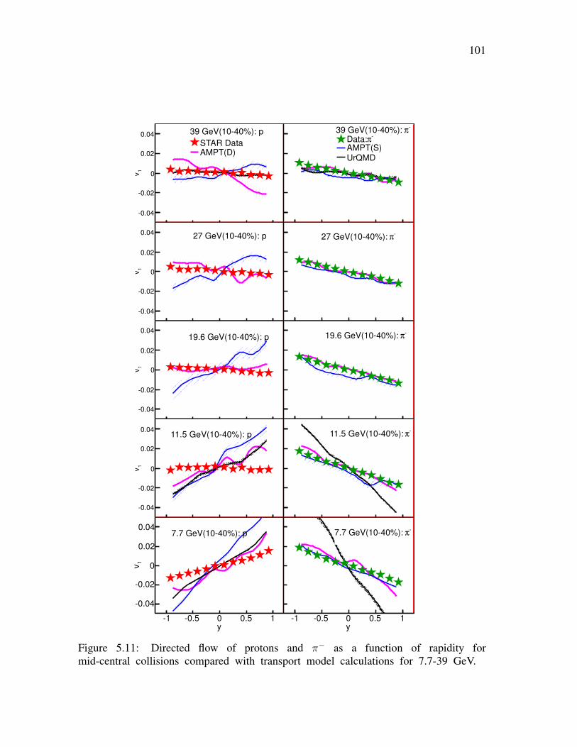
101

1 0.5 0 0.5 1

1v

0.04

0.02

0

0.02

0.04 39 GeV(1040%): p

STAR DataAMPT(D)

1 0.5 0 0.5 1

1v

0.04

0.02

0

0.02

0.04 27 GeV(1040%): p

1 0.5 0 0.5 1

1v

0.04

0.02

0

0.02

0.0419.6 GeV(1040%): p

1 0.5 0 0.5 1

1v

0.04

0.02

0

0.02

0.0411.5 GeV(1040%): p

y1 0.5 0 0.5 1

1v

0.04

0.02

0

0.02

0.047.7 GeV(1040%): p

1 0.5 0 0.5 1

0.04

0.02

0

0.02

0.04

π39 GeV(1040%):

πData:AMPT(S)UrQMD

1 0.5 0 0.5 1

0.04

0.02

0

0.02

0.04 π27 GeV(1040%):

1 0.5 0 0.5 1

0.04

0.02

0

0.02

0.04 π19.6 GeV(1040%):

1 0.5 0 0.5 1

0.04

0.02

0

0.02

0.04 π11.5 GeV(1040%):

y1 0.5 0 0.5 1

0.04

0.02

0

0.02

0.04 π7.7 GeV(1040%):

Figure 5.11: Directed flow of protons and π− as a function of rapidity formid-central collisions compared with transport model calculations for 7.7-39 GeV.

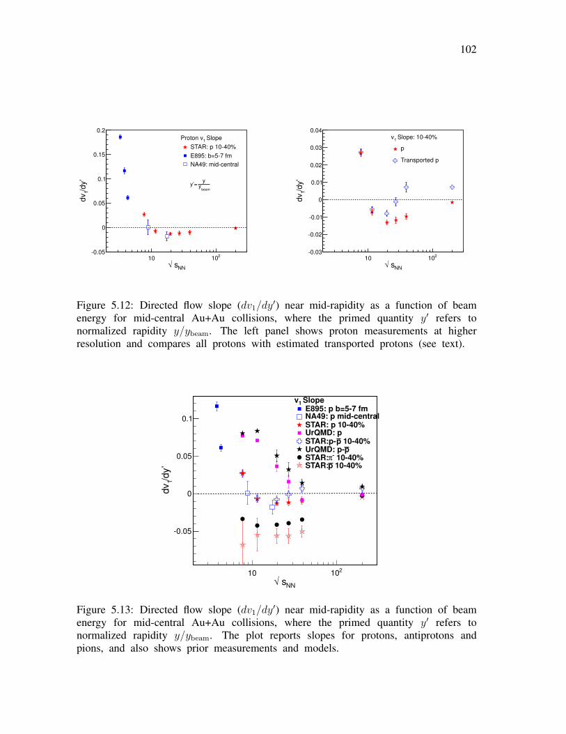
102

NN s√10

210

/dy’

1d

v

0.05

0

0.05

0.1

0.15

0.2

beamy

yy’=

Slope1

Proton v

STAR: p 1040%

E895: b=57 fm

NA49: midcentral

NN s√10

210

/dy’

1d

v

0.03

0.02

0.01

0

0.01

0.02

0.03

0.04 Slope: 1040%

1v

p

Transported p

Figure 5.12: Directed flow slope (dv1/dy′) near mid-rapidity as a function of beam

energy for mid-central Au+Au collisions, where the primed quantity y′ refers tonormalized rapidity y/ybeam. The left panel shows proton measurements at higherresolution and compares all protons with estimated transported protons (see text).

NN s√10 210

/dy’

1dv

0.05

0

0.05

0.1

Slope1vE895: p b=57 fm NA49: p midcentral STAR: p 1040% UrQMD: p

1040% pSTAR:ppUrQMD: p

1040% πSTAR: 1040% pSTAR:

Figure 5.13: Directed flow slope (dv1/dy′) near mid-rapidity as a function of beam

energy for mid-central Au+Au collisions, where the primed quantity y′ refers tonormalized rapidity y/ybeam. The plot reports slopes for protons, antiprotons andpions, and also shows prior measurements and models.

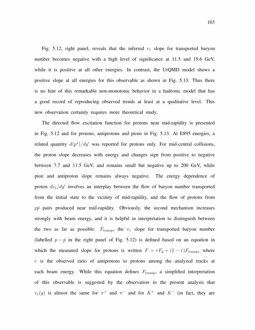
103

Fig. 5.12, right panel, reveals that the inferred v1 slope for transported baryon

number becomes negative with a high level of significance at 11.5 and 19.6 GeV,

while it is positive at all other energies. In contrast, the UrQMD model shows a

positive slope at all energies for this observable as shown in Fig. 5.13. Thus there

is no hint of this remarkable non-monotonic behavior in a hadronic model that has

a good record of reproducing observed trends at least at a qualitative level. This

new observation certainly requires more theoretical study.

The directed flow excitation function for protons near mid-rapidity is presented

in Fig. 5.12 and for protons, antiprotons and pions in Fig. 5.13. At E895 energies, a

related quantity d〈px〉/dy′ was reported for protons only. For mid-central collisions,

the proton slope decreases with energy and changes sign from positive to negative

between 7.7 and 11.5 GeV, and remains small but negative up to 200 GeV, while

pion and antiproton slope remains always negative. The energy dependence of

proton dv1/dy′ involves an interplay between the flow of baryon number transported

from the initial state to the vicinity of mid-rapidity, and the flow of protons from

pp pairs produced near mid-rapidity. Obviously, the second mechanism increases

strongly with beam energy, and it is helpful in interpretation to distinguish between

the two as far as possible. Ftransp, the v1 slope for transported baryon number

(labelled p− p in the right panel of Fig. 5.12) is defined based on an equation in

which the measured slope for protons is written F = rFp + (1 − r)Ftransp, where

r is the observed ratio of antiprotons to protons among the analyzed tracks at

each beam energy. While this equation defines Ftransp, a simplified interpretation

of this observable is suggested by the observation in the present analysis that

v1(y) is almost the same for π+ and π− and for K+ and K− (in fact, they are

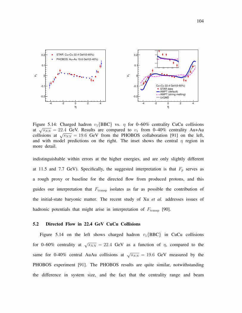
104

η

4 2 0 2 4

1v

0.2

0.1

0

0.1

0.2 STAR: Cu+Cu 22.4 GeV(060%)

PHOBOS: Au+Au 19.6 GeV(040%)

η

4 2 0 2 4

1v

0.2

0.1

0

0.1

0.2

Cu+Cu 22.4 GeV(060%)

STAR data AMPT (default)AMPT (string melting)

UrQMD

1 0.5 0 0.5 10.02

0.01

0

0.01

0.02

Figure 5.14: Charged hadron v1{BBC} vs. η for 0–60% centrality CuCu collisionsat√sNN = 22.4 GeV. Results are compared to v1 from 0–40% centrality Au+Au

collisions at√sNN = 19.6 GeV from the PHOBOS collaboration [91] on the left,

and with model predictions on the right. The inset shows the central η region inmore detail.

indistinguishable within errors at the higher energies, and are only slightly different

at 11.5 and 7.7 GeV). Specifically, the suggested interpretation is that Fp serves as

a rough proxy or baseline for the directed flow from produced protons, and this

guides our interpretation that Ftransp isolates as far as possible the contribution of

the initial-state baryonic matter. The recent study of Xu et al. addresses issues of

hadronic potentials that might arise in interpretation of Ftransp [90].

5.2 Directed Flow in 22.4 GeV CuCu Collisions

Figure 5.14 on the left shows charged hadron v1{BBC} in CuCu collisions

for 0–60% centrality at√sNN = 22.4 GeV as a function of η, compared to the

same for 0-40% central AuAu collisions at√sNN = 19.6 GeV measured by the

PHOBOS experiment [91]. The PHOBOS results are quite similar, notwithstanding

the difference in system size, and the fact that the centrality range and beam

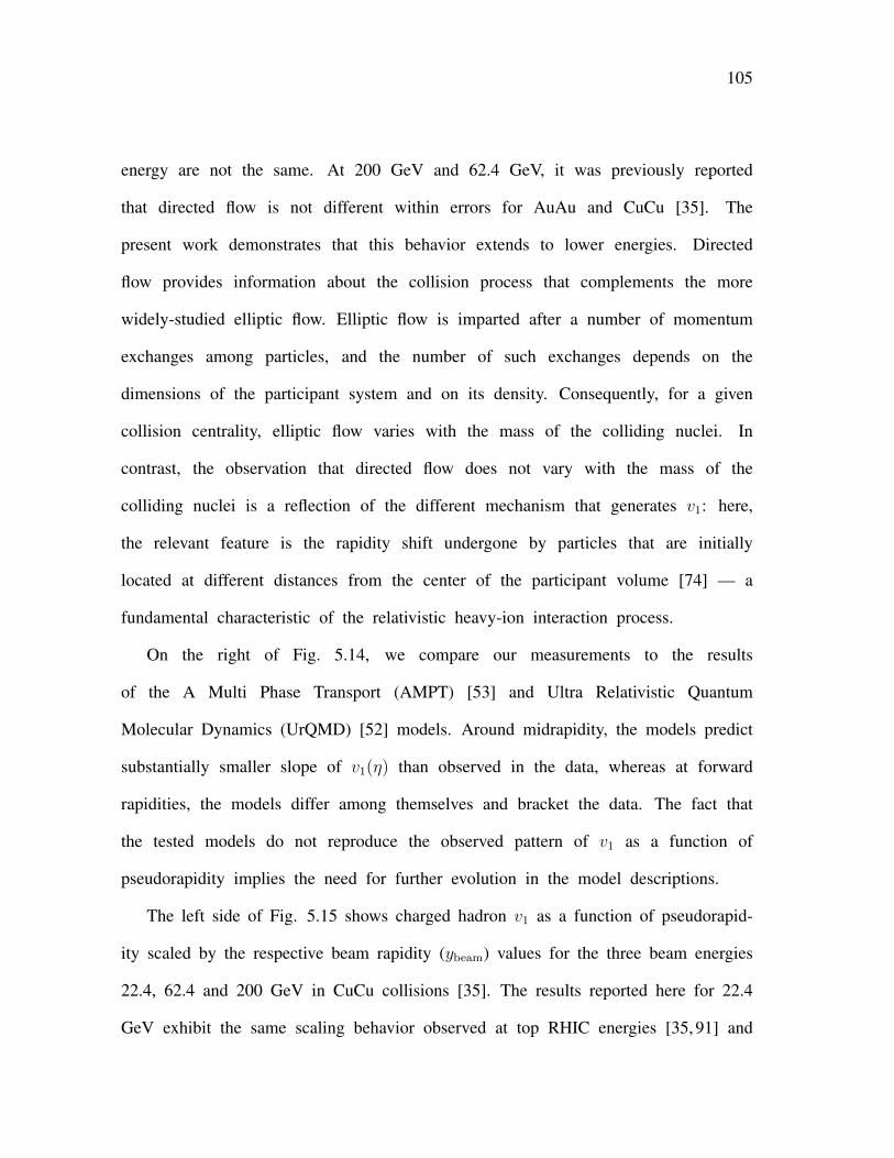
105

energy are not the same. At 200 GeV and 62.4 GeV, it was previously reported

that directed flow is not different within errors for AuAu and CuCu [35]. The

present work demonstrates that this behavior extends to lower energies. Directed

flow provides information about the collision process that complements the more

widely-studied elliptic flow. Elliptic flow is imparted after a number of momentum

exchanges among particles, and the number of such exchanges depends on the

dimensions of the participant system and on its density. Consequently, for a given

collision centrality, elliptic flow varies with the mass of the colliding nuclei. In

contrast, the observation that directed flow does not vary with the mass of the

colliding nuclei is a reflection of the different mechanism that generates v1: here,

the relevant feature is the rapidity shift undergone by particles that are initially

located at different distances from the center of the participant volume [74] — a

fundamental characteristic of the relativistic heavy-ion interaction process.

On the right of Fig. 5.14, we compare our measurements to the results

of the A Multi Phase Transport (AMPT) [53] and Ultra Relativistic Quantum

Molecular Dynamics (UrQMD) [52] models. Around midrapidity, the models predict

substantially smaller slope of v1(η) than observed in the data, whereas at forward

rapidities, the models differ among themselves and bracket the data. The fact that

the tested models do not reproduce the observed pattern of v1 as a function of

pseudorapidity implies the need for further evolution in the model descriptions.

The left side of Fig. 5.15 shows charged hadron v1 as a function of pseudorapid-

ity scaled by the respective beam rapidity (ybeam) values for the three beam energies

22.4, 62.4 and 200 GeV in CuCu collisions [35]. The results reported here for 22.4

GeV exhibit the same scaling behavior observed at top RHIC energies [35, 91] and

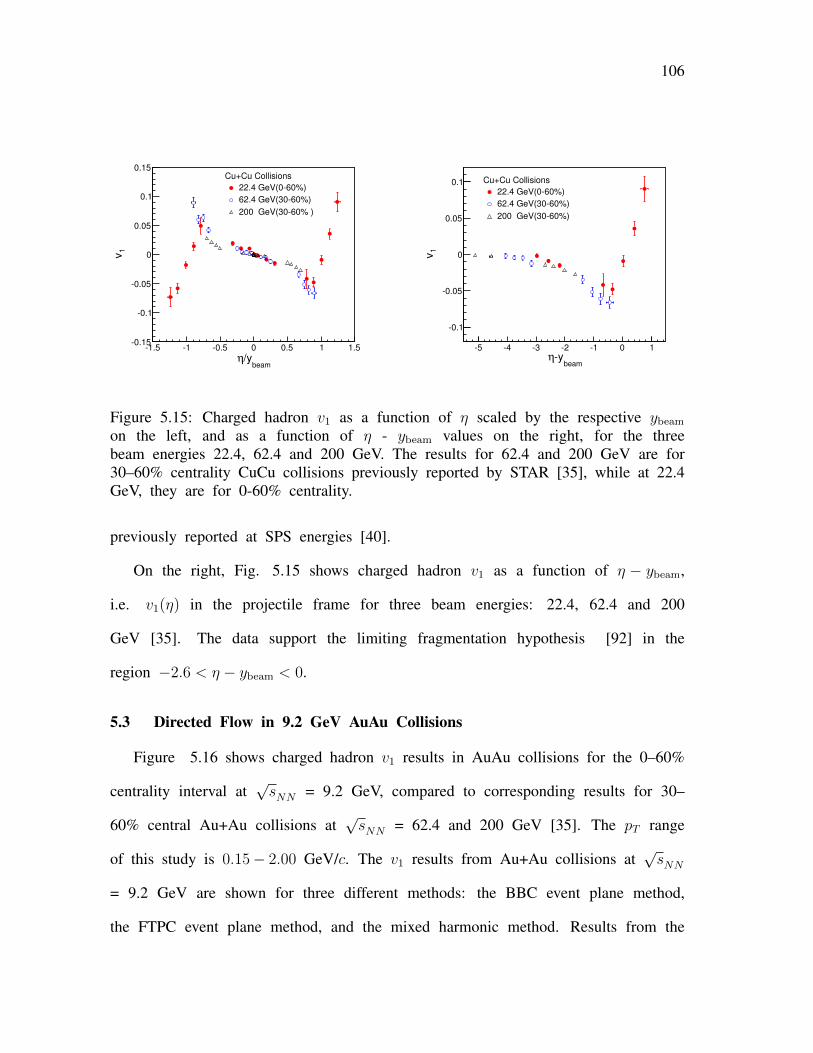
106

beam/yη

1.5 1 0.5 0 0.5 1 1.5

1v

0.15

0.1

0.05

0

0.05

0.1

0.15Cu+Cu Collisions

22.4 GeV(060%)

62.4 GeV(3060%)

200 GeV(3060% )

beamyη

5 4 3 2 1 0 1

1v

0.1

0.05

0

0.05

0.1 Cu+Cu Collisions

22.4 GeV(060%)

62.4 GeV(3060%)

200 GeV(3060%)

Figure 5.15: Charged hadron v1 as a function of η scaled by the respective ybeam

on the left, and as a function of η - ybeam values on the right, for the threebeam energies 22.4, 62.4 and 200 GeV. The results for 62.4 and 200 GeV are for30–60% centrality CuCu collisions previously reported by STAR [35], while at 22.4GeV, they are for 0-60% centrality.

previously reported at SPS energies [40].

On the right, Fig. 5.15 shows charged hadron v1 as a function of η − ybeam,

i.e. v1(η) in the projectile frame for three beam energies: 22.4, 62.4 and 200

GeV [35]. The data support the limiting fragmentation hypothesis [92] in the

region −2.6 < η − ybeam < 0.

5.3 Directed Flow in 9.2 GeV AuAu Collisions

Figure 5.16 shows charged hadron v1 results in AuAu collisions for the 0–60%

centrality interval at√sNN = 9.2 GeV, compared to corresponding results for 30–

60% central Au+Au collisions at√sNN = 62.4 and 200 GeV [35]. The pT range

of this study is 0.15− 2.00 GeV/c. The v1 results from Au+Au collisions at√sNN

= 9.2 GeV are shown for three different methods: the BBC event plane method,

the FTPC event plane method, and the mixed harmonic method. Results from the

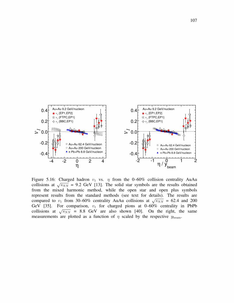
107

η-4 -2 0 2 4

1v

-0.4

-0.2

0.0

0.2

0.4 {EP1,EP2}

1v

{FTPC,EP1}1

v

{BBC,EP1}1

v

Au+Au 62.4 GeV/nucleon

Au+Au 200 GeV/nucleon

Pb+Pb 8.8 GeV/nucleonπ


beam / yη

-2 -1 0 1 2

1v

-0.4

-0.2

0.0

0.2

0.4 {EP1,EP2}

1v

{FTPC,EP1}1

v

{BBC,EP1}1

v


Au+Au 200 GeV/nucleon

Pb+Pb 8.8 GeV/nucleonπ


Figure 5.16: Charged hadron v1 vs. η from the 0–60% collision centrality AuAucollisions at

√sNN = 9.2 GeV [13]. The solid star symbols are the results obtained

from the mixed harmonic method, while the open star and open plus symbolsrepresent results from the standard methods (see text for details). The results arecompared to v1 from 30–60% centrality AuAu collisions at

√sNN = 62.4 and 200

GeV [35]. For comparison, v1 for charged pions at 0–60% centrality in PbPbcollisions at

√sNN = 8.8 GeV are also shown [40]. On the right, the same

measurements are plotted as a function of η scaled by the respective ybeam.

108

three methods are consistent within the error bars. These results are also compared

with v1 for charged pions in Pb+Pb collisions at√sNN = 8.8 GeV measured by

NA49 [40]. At midrapidity, all results are comparable. At forward rapidity (|η| > 2),

the trend of v1 for higher√sNN (62.4 and 200 GeV) appears to be different from

that for√sNN = 9.2 GeV. This can be explained by contributions from spectator

protons to the directed flow signal at large |η|. The beam rapidities (ybeam) for√sNN = 9.2, 62.4, and 200 GeV are 2.3, 4.2, and 5.4, respectively. With η divided

by the respective ybeam values, all the v1 measurements follow a common trend for

the measured pseudorapidity range.


When the event plane for a directed flow measurement is determined from a

detector that is not symmetric around η = 0, we need to account for correlations

due to momentum conservation [78]. The desired BBC η symmetry is present for

our v1 analysis in the η region of the central TPC, but is a source of possible

concern for the FTPC η region. The overlap in η acceptance between the BBC

and FTPC is only partial, and therefore it is feasible to compare v1{BBC}full, using

the combined full event plane based on both BBCs, with v1{BBC}sub, using a

single BBC sub-event plane for 2.5 < |η| < 3.3. We find that the difference is less

than 10%, and an extrapolated average correction has been applied to v1{BBC} for

|η| > 3.3.

The measured v1 has to be anti-symmetric about mid-pseudorapidity within

statistical errors. Any difference is due to systematic uncertainties. Previous detailed

studies point to the maximum forward-backward difference as a viable estimate

of the overall systematic uncertainty when the pseudorapidity gap is large [35].

109

The difference in measured value with respect to the event planes reconstructed in

different detectors also gives an estimate of the systematic error. We estimate the

difference between v1{BBC} and v1{FTPC}, and this difference is less than 2%

in TPC region and 5% in FTPC region. We estimate the systematic uncertainty

on event plane flattening methods by the variance between them and find it to be

negligible (below 1%).

Results for pions and protons are not corrected for feed-down from weak decays.

The systematic uncertainties arising from particle misidentification and detector

inefficiency are estimated by varying the event and track cuts, and are concluded to

be at the level of about 5%. Because of the large pseudorapidity gap between the

BBC and TPC, the non-flow contribution in v1{BBC} is negligible. We conclude

that the overall systematic uncertainty in our determination of v1 is approximately

15% in the FTPC region, and 10% in the central TPC region.

5.5 Summary

I presented measurements of directed flow of charged particles and of charged

pions, kaons, protons and antiprotons for AuAu collisions at 7.7, 11.5, 19.6, 27

and 39 GeV. I also present directed flow of charged particles for 22.4 GeV

CuCu collisions and 9.2 GeV AuAu collisions. The centrality dependence of

the charged hadron directed flow as a function of pseudorapidity and transverse

momentum observed at these energies is similar to results observed at the top RHIC

energy. We observe that v1(η/ybeam) for 30-60% central collisions lies close to a

single common curve for all beam energies as previously reported by NA49 [40]

and STAR [74]. Beam energy scaling of charged hadron v1 as a function of

(η − ybeam) for 30-60% central collisions resembles the pattern previously reported

110

by PHOBOS [91]. These approximate scaling behaviors are equally observed in

AuAu collisions as well as CuCu collisions. These observations support the limiting

fragmentation hypothesis [92].

At 200 GeV and 62.4 GeV, it was previously reported that directed flow is not

different within errors for AuAu and CuCu [35]. We find that this behavior extends

to lower energies, as evident from comparison between CuCu 22 GeV and AuAu

19.6 GeV collisions [74].

For charged particles in 0-30% central collisions, we observe a local minimum

of integrated (0.2 < pT < 2.0 GeV/c and |η| < 1.0) directed flow above 11.5 GeV.

This type of observation has been argued to be of interest in studying the softest

point in the Nuclear Equation of State [81, 84]. The mean transverse momentum

also shows a similar behavior. The minimum in directed flow survives when scaled

with mean transverse momentum, but this alone cannot exclude the possibility of

a connection between them. This is a very interesting observation and further

investigation is necessary to fully understand it.

We report directed flow of identified particles. Differences in directed flow

between positive and negative hadrons, especially for protons and antiprotons, is

observed and this difference becomes smaller for higher beam energies. For mid-

central collisions, the proton v1 slope in the mid-rapidity region changes sign from

positive to negative between 7.7 and 11.5 GeV and remains small but negative

up to 200 GeV, while the slope for pions, kaons and antiprotons remains always

negative. Based on transport model comparisons, the observed trends in these data

above 11.5 GeV can qualitatively be understood in terms of anisotropic emission of

produced particles from a tilted disk. A striking observation is that the v1 slope

111

for net protons, which is an estimate of the directed flow contribution from baryon

number transported to the midrapidity region, changes sign twice within the energy

range studied here [8]. This result is qualitatively different from transport model

calculations, which exhibit a monotonic trend with no sign reversal.

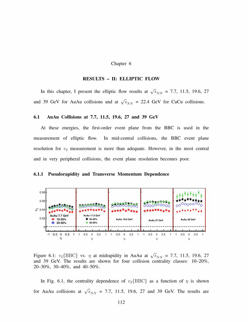
Chapter 6

RESULTS – II: ELLIPTIC FLOW

In this chapter, I present the elliptic flow results at√sNN = 7.7, 11.5, 19.6, 27

and 39 GeV for AuAu collisions and at√sNN = 22.4 GeV for CuCu collisions.

6.1 AuAu Collisions at 7.7, 11.5, 19.6, 27 and 39 GeV

At these energies, the first-order event plane from the BBC is used in the

measurement of elliptic flow. In mid-central collisions, the BBC event plane

resolution for v2 measurement is more than adequate. However, in the most central

and in very peripheral collisions, the event plane resolution becomes poor.

6.1.1 Pseudorapidity and Transverse Momentum Dependence

η

1 0.5 0 0.5 1

2v

0

0.02

0.04

0.06

0.08

AuAu 7.7 GeV

1020%

2030%

η

1 0.5 0 0.5 1

0

0.02

0.04

0.06

0.08

AuAu 11.5 GeV

3040%

4050%

η

1 0.5 0 0.5 1

0

0.02

0.04

0.06

0.08

AuAu 19.6 GeV

η

1 0.5 0 0.5 1

0

0.02

0.04

0.06

0.08

AuAu 27 GeV

η

1 0.5 0 0.5 1

0

0.02

0.04

0.06

0.08

AuAu 39 GeV

Figure 6.1: v2{BBC} vs. η at midrapidity in AuAu at√sNN = 7.7, 11.5, 19.6, 27

and 39 GeV. The results are shown for four collision centrality classes: 10–20%,20–30%, 30–40%, and 40–50%.

In Fig. 6.1, the centrality dependence of v2{BBC} as a function of η is shown

for AuAu collisions at√sNN = 7.7, 11.5, 19.6, 27 and 39 GeV. The results are

112

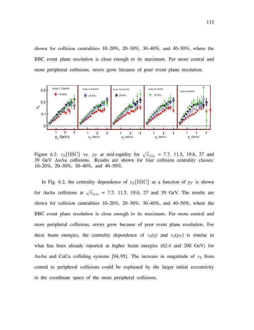
113

shown for collision centralities 10–20%, 20–30%, 30–40%, and 40–50%, where the

BBC event plane resolution is close enough to its maximum. For more central and

more peripheral collisions, errors grow because of poor event plane resolution.

GeV/cT

p

1 2 3

2v

0

0.1

0.2

0.3AuAu 7.7 GeV%

1020%

GeV/cT

p

1 2 3

0

0.05

0.1

0.15

0.2

0.25

0.3AuAu 11.5 GeV%

2030%

GeV/cT

p

1 2 3

0

0.05

0.1

0.15

0.2

0.25

0.3 AuAu 19.6 GeV%

3040%

GeV/cT

p

1 2 3

0

0.05

0.1

0.15

0.2

0.25

0.3AuAu 27 GeV%

4050%

GeV/cT

p

1 2 3

0

0.05

0.1

0.15

0.2

0.25

0.3

AuAu 39 GeV%

Figure 6.2: v2{BBC} vs. pT at mid-rapidity for√sNN = 7.7, 11.5, 19.6, 27 and

39 GeV AuAu collisions. Results are shown for four collision centrality classes:10–20%, 20–30%, 30–40%, and 40–50%.

In Fig. 6.2, the centrality dependence of v2{BBC} as a function of pT is shown

for AuAu collisions at√sNN = 7.7, 11.5, 19.6, 27 and 39 GeV. The results are

shown for collision centralities 10–20%, 20–30%, 30–40%, and 40–50%, where the

BBC event plane resolution is close enough to its maximum. For more central and

more peripheral collisions, errors grow because of poor event plane resolution. For

these beam energies, the centrality dependence of v2(η) and v2(pT ) is similar to

what has been already reported at higher beam energies (62.4 and 200 GeV) for

AuAu and CuCu colliding systems [94, 95]. The increase in magnitude of v2 from

central to peripheral collisions could be explained by the larger initial eccentricity

in the coordinate space of the more peripheral collisions.

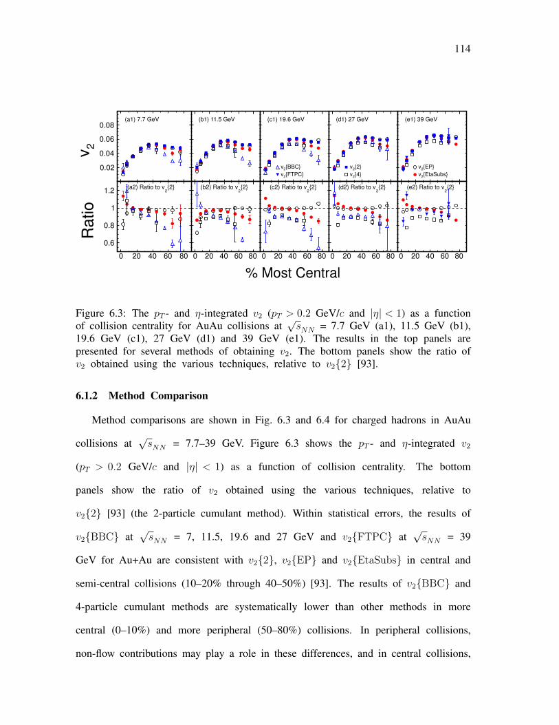
114

0.02

0.04

0.06

0.08(a1) 7.7 GeV

0.02

0.04

0.06

0.08(b1) 11.5 GeV

0.02

0.04

0.06

0.08(c1) 19.6 GeV

{BBC}2v

{FTPC}2v0.02

0.04

0.06

0.08(d1) 27 GeV

{2}2v

{4}2v0.02

0.04

0.06

0.08(e1) 39 GeV

{EP}2v

{EtaSubs}2v

0 20 40 60 80

0.6

0.8

1

1.2{2}

2(a2) Ratio to v

0 20 40 60 80

0.6

0.8

1

1.2{2}

2(b2) Ratio to v

0 20 40 60 80

0.6

0.8

1

1.2{2}

2(c2) Ratio to v

0 20 40 60 80

0.6

0.8

1

1.2{2}

2(d2) Ratio to v

0 20 40 60 80

0.6

0.8

1

1.2{2}

2(e2) Ratio to v

% Most Central

2v

Ratio

Figure 6.3: The pT - and η-integrated v2 (pT > 0.2 GeV/c and |η| < 1) as a functionof collision centrality for AuAu collisions at

√sNN = 7.7 GeV (a1), 11.5 GeV (b1),

19.6 GeV (c1), 27 GeV (d1) and 39 GeV (e1). The results in the top panels arepresented for several methods of obtaining v2. The bottom panels show the ratio ofv2 obtained using the various techniques, relative to v2{2} [93].

6.1.2 Method Comparison

Method comparisons are shown in Fig. 6.3 and 6.4 for charged hadrons in AuAu

collisions at√sNN = 7.7–39 GeV. Figure 6.3 shows the pT - and η-integrated v2

(pT > 0.2 GeV/c and |η| < 1) as a function of collision centrality. The bottom

panels show the ratio of v2 obtained using the various techniques, relative to

v2{2} [93] (the 2-particle cumulant method). Within statistical errors, the results of

v2{BBC} at√sNN = 7, 11.5, 19.6 and 27 GeV and v2{FTPC} at

√sNN = 39

GeV for Au+Au are consistent with v2{2}, v2{EP} and v2{EtaSubs} in central and

semi-central collisions (10–20% through 40–50%) [93]. The results of v2{BBC} and

4-particle cumulant methods are systematically lower than other methods in more

central (0–10%) and more peripheral (50–80%) collisions. In peripheral collisions,

non-flow contributions may play a role in these differences, and in central collisions,

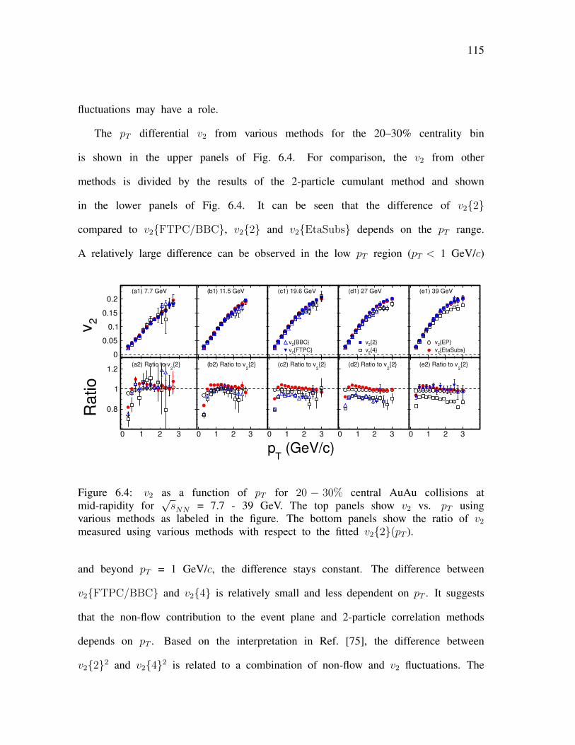
115

fluctuations may have a role.

The pT differential v2 from various methods for the 20–30% centrality bin

is shown in the upper panels of Fig. 6.4. For comparison, the v2 from other

methods is divided by the results of the 2-particle cumulant method and shown

in the lower panels of Fig. 6.4. It can be seen that the difference of v2{2}

compared to v2{FTPC/BBC}, v2{2} and v2{EtaSubs} depends on the pT range.

A relatively large difference can be observed in the low pT region (pT < 1 GeV/c)

0

0.05

0.1

0.15

0.2(a1) 7.7 GeV

0

0.05

0.1

0.15

0.2

(b1) 11.5 GeV

0

0.05

0.1

0.15

0.2

(c1) 19.6 GeV

{BBC}2v

{FTPC}2v0

0.05

0.1

0.15

0.2

(d1) 27 GeV

{2}2v

{4}2v0

0.05

0.1

0.15

0.2

(e1) 39 GeV

{EP}2v

{EtaSubs}2v

0 1 2 3

0.8

1

1.2{2}

2(a2) Ratio to v

0 1 2 3

0.8

1

1.2{2}

2(b2) Ratio to v

0 1 2 3

0.8

1

1.2{2}

2(c2) Ratio to v

0 1 2 3

0.8

1

1.2{2}

2(d2) Ratio to v

0 1 2 3

0.8

1

1.2{2}

2(e2) Ratio to v

(GeV/c)T

p

2v

Ratio

Figure 6.4: v2 as a function of pT for 20 − 30% central AuAu collisions atmid-rapidity for

√sNN = 7.7 - 39 GeV. The top panels show v2 vs. pT using

various methods as labeled in the figure. The bottom panels show the ratio of v2

measured using various methods with respect to the fitted v2{2}(pT ).

and beyond pT = 1 GeV/c, the difference stays constant. The difference between

v2{FTPC/BBC} and v2{4} is relatively small and less dependent on pT . It suggests

that the non-flow contribution to the event plane and 2-particle correlation methods

depends on pT . Based on the interpretation in Ref. [75], the difference between

v2{2}2 and v2{4}2 is related to a combination of non-flow and v2 fluctuations. The

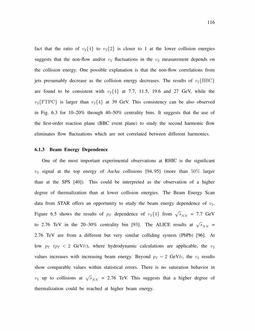
116

fact that the ratio of v2{4} to v2{2} is closer to 1 at the lower collision energies

suggests that the non-flow and/or v2 fluctuations in the v2 measurement depends on

the collision energy. One possible explanation is that the non-flow correlations from

jets presumably decrease as the collision energy decreases. The results of v2{BBC}

are found to be consistent with v2{4} at 7.7, 11.5, 19.6 and 27 GeV, while the

v2{FTPC} is larger than v2{4} at 39 GeV. This consistency can be also observed

in Fig. 6.3 for 10–20% through 40–50% centrality bins. It suggests that the use of

the first-order reaction plane (BBC event plane) to study the second harmonic flow

eliminates flow fluctuations which are not correlated between different harmonics.

6.1.3 Beam Energy Dependence

One of the most important experimental observations at RHIC is the significant

v2 signal at the top energy of AuAu collisions [94, 95] (more than 50% larger

than at the SPS [40]). This could be interpreted as the observation of a higher

degree of thermalization than at lower collision energies. The Beam Energy Scan

data from STAR offers an opportunity to study the beam energy dependence of v2.

Figure 6.5 shows the results of pT dependence of v2{4} from√sNN = 7.7 GeV

to 2.76 TeV in the 20–30% centrality bin [93]. The ALICE results at√sNN =

2.76 TeV are from a different but very similar colliding system (PbPb) [96]. At

low pT (pT < 2 GeV/c), where hydrodynamic calculations are applicable, the v2

values increases with increasing beam energy. Beyond pT = 2 GeV/c, the v2 results

show comparable values within statistical errors. There is no saturation behavior in

v2 up to collisions at√sNN = 2.76 TeV. This suggests that a higher degree of

thermalization could be reached at higher beam energy.

117

0

0.05

0.1

0.15

0.2(a1) 10 20%Fit to 200 GeV data

0

0.05

0.1

0.15

0.2

(b1) 20 30%

2.76 TeV

200 GeV

62.4 GeV

39 GeV0

0.05

0.1

0.15

0.2

(c1) 30 40%

27 GeV

19.6 GeV

11.5 GeV

7.7 GeV

0 1 2 3

0.6

0.8

1

1.2

1.4 (a2) Ratio to fit function

0 1 2 3

0.6

0.8

1

1.2

1.4 (b2) Ratio to fit function

0 1 2 3

0.6

0.8

1

1.2

1.4 (c2) Ratio to fit function

(GeV/c)T

p

2v

Ra

tio

Figure 6.5: The top panels show v2{4} vs. pT at mid-rapidity for various beamenergies (

√sNN = 7.7 GeV to 2.76 TeV). The results for

√sNN = 7.7 to 200 GeV

are for AuAu collisions and those for 2.76 TeV are for Pb + Pb collisions. Thered line shows a fit to the results from AuAu collisions at

√sNN = 200 GeV. The

bottom panels show the ratio of v2{4} vs. pT for all√sNN with respect to this

fitted curve. The results are shown for three collision centrality classes: 10–20%(a), 20–30% (b) and 30–40% (c) [93].

6.2 CuCu Collisions at 22.4 GeV

In the elliptic flow measurement, we have used the η sub-event method with a

gap of 0.3 units in pseudorapidity (η), such a gap suppresses short-range correlations

such as Bose-Einstein interference and Coulomb final-state interactions. To study

possible systematic effects associated with short-range non-flow correlations, a four-

particle cumulant [75] analysis v2{4} as a function of centrality has been investigated.

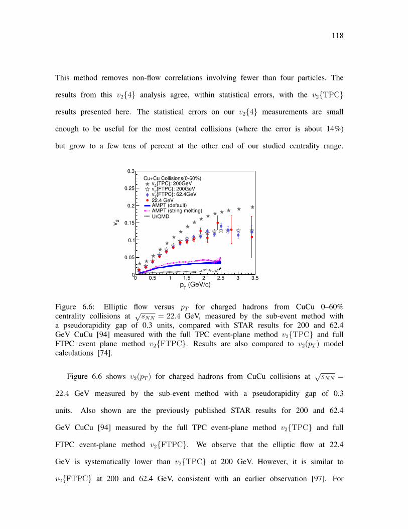
118

This method removes non-flow correlations involving fewer than four particles. The

results from this v2{4} analysis agree, within statistical errors, with the v2{TPC}

results presented here. The statistical errors on our v2{4} measurements are small

enough to be useful for the most central collisions (where the error is about 14%)

but grow to a few tens of percent at the other end of our studied centrality range.

(GeV/c)T

p0 0.5 1 1.5 2 2.5 3 3.5

2v

0

0.05

0.1

0.15

0.2

0.25

0.3

Cu+Cu Collisions(060%): 200GeV {TPC}

2v

: 200GeV {FTPC}2

v: 62.4GeV {FTPC}

2v22.4 GeVAMPT (default)AMPT (string melting)UrQMD

Figure 6.6: Elliptic flow versus pT for charged hadrons from CuCu 0–60%centrality collisions at

√sNN = 22.4 GeV, measured by the sub-event method with

a pseudorapidity gap of 0.3 units, compared with STAR results for 200 and 62.4GeV CuCu [94] measured with the full TPC event-plane method v2{TPC} and fullFTPC event plane method v2{FTPC}. Results are also compared to v2(pT ) modelcalculations [74].

Figure 6.6 shows v2(pT ) for charged hadrons from CuCu collisions at√sNN =

22.4 GeV measured by the sub-event method with a pseudorapidity gap of 0.3

units. Also shown are the previously published STAR results for 200 and 62.4

GeV CuCu [94] measured by the full TPC event-plane method v2{TPC} and full

FTPC event-plane method v2{FTPC}. We observe that the elliptic flow at 22.4

GeV is systematically lower than v2{TPC} at 200 GeV. However, it is similar to

v2{FTPC} at 200 and 62.4 GeV, consistent with an earlier observation [97]. For

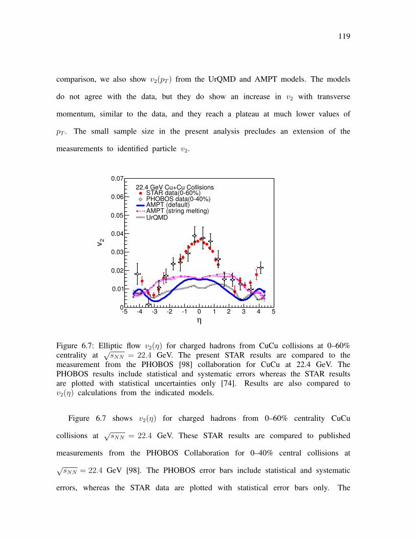
119

comparison, we also show v2(pT ) from the UrQMD and AMPT models. The models

do not agree with the data, but they do show an increase in v2 with transverse

momentum, similar to the data, and they reach a plateau at much lower values of

pT . The small sample size in the present analysis precludes an extension of the

measurements to identified particle v2.

η

5 4 3 2 1 0 1 2 3 4 5

2v

0

0.01

0.02

0.03

0.04

0.05

0.06

0.07

22.4 GeV Cu+Cu CollisionsSTAR data(060%) PHOBOS data(040%)AMPT (default)AMPT (string melting)UrQMD

Figure 6.7: Elliptic flow v2(η) for charged hadrons from CuCu collisions at 0–60%centrality at

√sNN = 22.4 GeV. The present STAR results are compared to the

measurement from the PHOBOS [98] collaboration for CuCu at 22.4 GeV. ThePHOBOS results include statistical and systematic errors whereas the STAR resultsare plotted with statistical uncertainties only [74]. Results are also compared tov2(η) calculations from the indicated models.

Figure 6.7 shows v2(η) for charged hadrons from 0–60% centrality CuCu

collisions at√sNN = 22.4 GeV. These STAR results are compared to published

measurements from the PHOBOS Collaboration for 0–40% central collisions at√sNN = 22.4 GeV [98]. The PHOBOS error bars include statistical and systematic

errors, whereas the STAR data are plotted with statistical error bars only. The

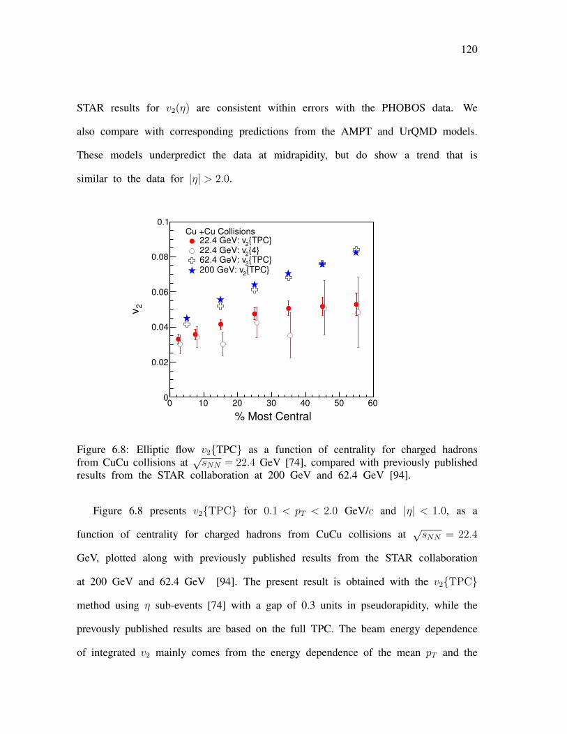
120

STAR results for v2(η) are consistent within errors with the PHOBOS data. We

also compare with corresponding predictions from the AMPT and UrQMD models.

These models underpredict the data at midrapidity, but do show a trend that is

similar to the data for |η| > 2.0.

% Most Central

0 10 20 30 40 50 60

2v

0

0.02

0.04

0.06

0.08

0.1Cu +Cu Collisions

{TPC}2

22.4 GeV: v{4}

222.4 GeV: v

{TPC}2

62.4 GeV: v{TPC}

2200 GeV: v

Figure 6.8: Elliptic flow v2{TPC} as a function of centrality for charged hadronsfrom CuCu collisions at

√sNN = 22.4 GeV [74], compared with previously published

results from the STAR collaboration at 200 GeV and 62.4 GeV [94].

Figure 6.8 presents v2{TPC} for 0.1 < pT < 2.0 GeV/c and |η| < 1.0, as a

function of centrality for charged hadrons from CuCu collisions at√sNN = 22.4

GeV, plotted along with previously published results from the STAR collaboration

at 200 GeV and 62.4 GeV [94]. The present result is obtained with the v2{TPC}

method using η sub-events [74] with a gap of 0.3 units in pseudorapidity, while the

prevously published results are based on the full TPC. The beam energy dependence

of integrated v2 mainly comes from the energy dependence of the mean pT and the

121

difference between the event plane reconstruction with and without a pseudorapidity

gap.


For AuAu collisions at 7.7, 11.5, 19.6, 27 and 39 GeV, the non-flow correlations

are highly suppressed in our v2{BBC} method because of the large η gap between

the TPC and BBC. Furthermore, we measure v2 with respect to the first-order

event plane, which suppresses contributions from flow fluctuations. Therefore these

measurements are very similar to the results from the four-particle cumulant method.

Estimated systematic uncertainty arising from event-plane flattening methods are

found to be negligible (below 1%). An additional 5% systematic uncertainty is

estimated by varying cut parameters (e.g. collision vertex position, the distance of

closest approach of tracks to the primary vertex, and the number of fit points used

for reconstruction of the tracks).

In CuCu collisions at 22.4 GeV, our measurements of elliptic flow are based on

the TPC event plane, v2{TPC}. Unlike in the case of v2{BBC}, we do not have

the advantage of a wide η gap to help ensure that non-flow background effects

are minimized. To study possible systematic effects associated with short-range

non-flow correlations, a four-particle cumulant [75] analysis v2{4} as a function

of centrality has been investigated. This method suppresses non-flow correlations

involving fewer than four particles. The statistical errors on our v2{4} measurements

are small enough to be useful for the most central collisions, but grow to a few

tens of percent at the other end of our studied centrality range. The v2{TPC} and

v2{4} measurements agree within statistical errors, although the observed systematic

difference, which might arise from non-flow effects, amounts to about 9% for the

122

0–10% most central collisions. In the v2{TPC} method, the η sub-event method

with a gap of 0.3 units in pseudorapidity (η) has been used. Such a gap suppresses

short-range correlations such as Bose-Einstein interference and Coulomb final-state

interactions. To estimate the non-flow contributions to the measurement of v2{TPC}

due to these short-range correlations, a systematic study has been performed with

variations in the resulting v2{TPC} induced by varying the event vertex selection

along the beam direction, by varying the DCA cut value, and by varying the size

of the pseudorapidity gap between the sub-events in the η sub-event method. Tests

of this type suggest that the systematic error on v2 is on the order of 10% [74].

6.4 Summary

I presented measurements of elliptic flow, v2{BBC}, in AuAu collisions at√sNN = 7.7, 11.5, 19.6, 27 and 39 GeV for charged hadrons at mid-rapidity. I

measured elliptic flow with respect to the first-order event plane reconstructed at

larger rapidity. This method is effective in suppressing non-flow and flow fluctuation

effects. The results from this method are consistent with the v2{4} method. This

method is very helpful to estimate the systematic uncertainties from non-flow effects

and flow fluctuations, by comparing these results to the other measurement methods

like v2{TPC} and 2-particle cumulant v2{2} methods, which are commonly used in

elliptic flow analysis. The centrality, η and pT dependence of v2 are similar to those

observed at higher RHIC beam energies. The integrated v2 signal increases from

central to mid central collisions, and it drops back down in peripheral collisions.

The comparison with AuAu collisions at higher RHIC energies (√sNN = 62.4 and

200 GeV) and at LHC (PbPb collisions at√sNN = 2.76 TeV) shows that the v2

values increase with increasing beam energy at low pT (pT < 2.0 GeV/c) where

123

hydrodynamic calculations are applicable.

Measurements of the elliptic flow for 22.4 GeV CuCu collisions are also

presented. We compare pT -integrated v2 with measurements at higher energies. The

pT dependence of the measured v2 at 22.4 GeV is similar to that at 62.4 and

200 GeV. Comparisons with UrQMD and AMPT models (the latter both with and

without string melting) do not agree with the present measurements [74].

Chapter 7

RESULTS – III: TRIANGULAR FLOW

In this chapter, I present the third harmonic coefficient for azimuthal anisotropy,

popularly known as triangular flow, for charged particles as a function of pseudo-

rapidity, transverse momentum and centrality, for AuAu collisions at√sNN = 200

GeV, based on data taken in 2004 (run IV). Triangular flow is a relatively new

observable and provides extra information concerning initial-state fluctuations, and

the subsequent evolution of the collision system [20, 43].

7.1 Centrality dependence

Figure 7.1 shows the width and amplitude of the wide Gaussian (introduced in

Chapter 4) as a function of centrality on the left, and as a function of pT for

centralities 0–5% and 30–40% on the right. Above pT = 0.8 GeV/c, the distribution

can be described by a single wide Gaussian. The amplitude increases with pT and

then saturates around pT = 3 GeV/c. The pT dependence of the width seems to

depend on centrality, with the 0–5% most central data showing first an increase and

then a gradual decrease, while at 30–40% centrality, the data appear to gradually

decrease for all pT .

The Fig. 7.2, left panel, shows the centrality dependence for pT -integrated v3 from

several different analyses: two-particle cumulants with a minimum pseudorapidity

separation of one unit between particles, v3{2} evaluated using the wide Gaussian

124

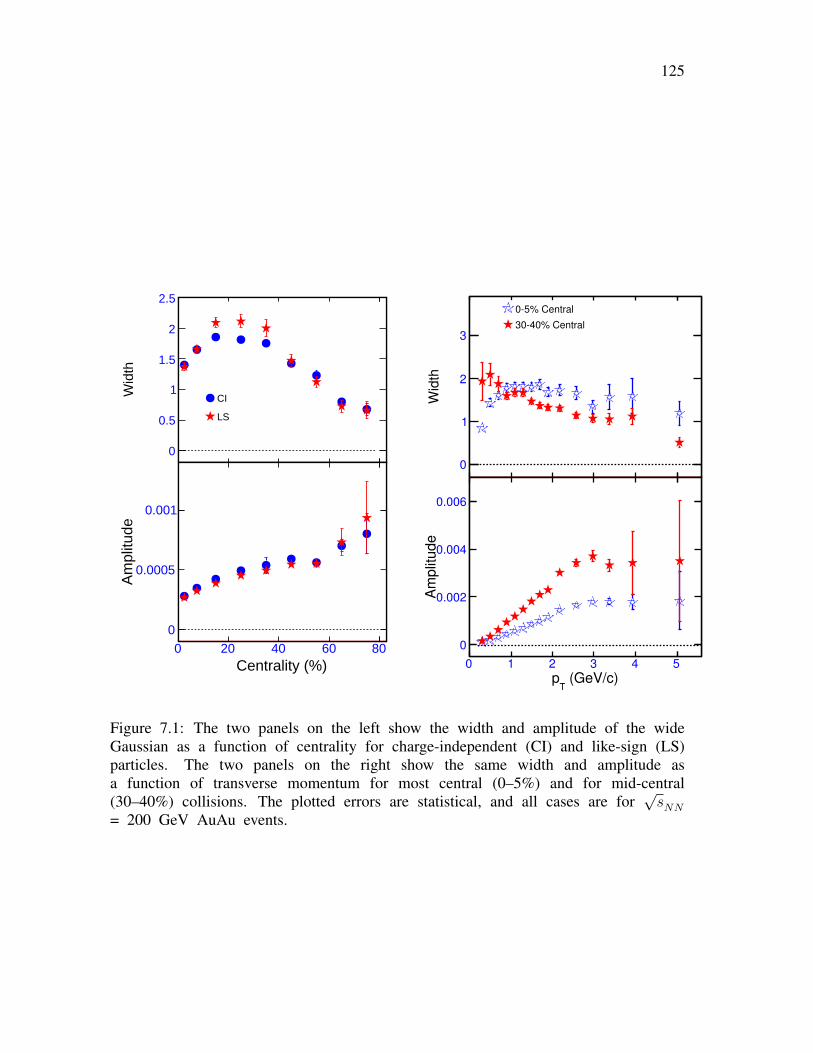
125

Centrality (%)0 20 40 60 80

Wid

th

0

0.5

1

1.5

2

2.5

CI

LS

Centrality (%)0 20 40 60 80

Am

plitu

de

0

0.0005

0.001

0 1 2 3 4 5

Wid

th

0

1

2

3

05% Central

3040% Central

(GeV/c)T

p0 1 2 3 4 5

Am

plit

ude

0

0.002

0.004

0.006

Figure 7.1: The two panels on the left show the width and amplitude of the wideGaussian as a function of centrality for charge-independent (CI) and like-sign (LS)particles. The two panels on the right show the same width and amplitude asa function of transverse momentum for most central (0–5%) and for mid-central(30–40%) collisions. The plotted errors are statistical, and all cases are for

√sNN

= 200 GeV AuAu events.

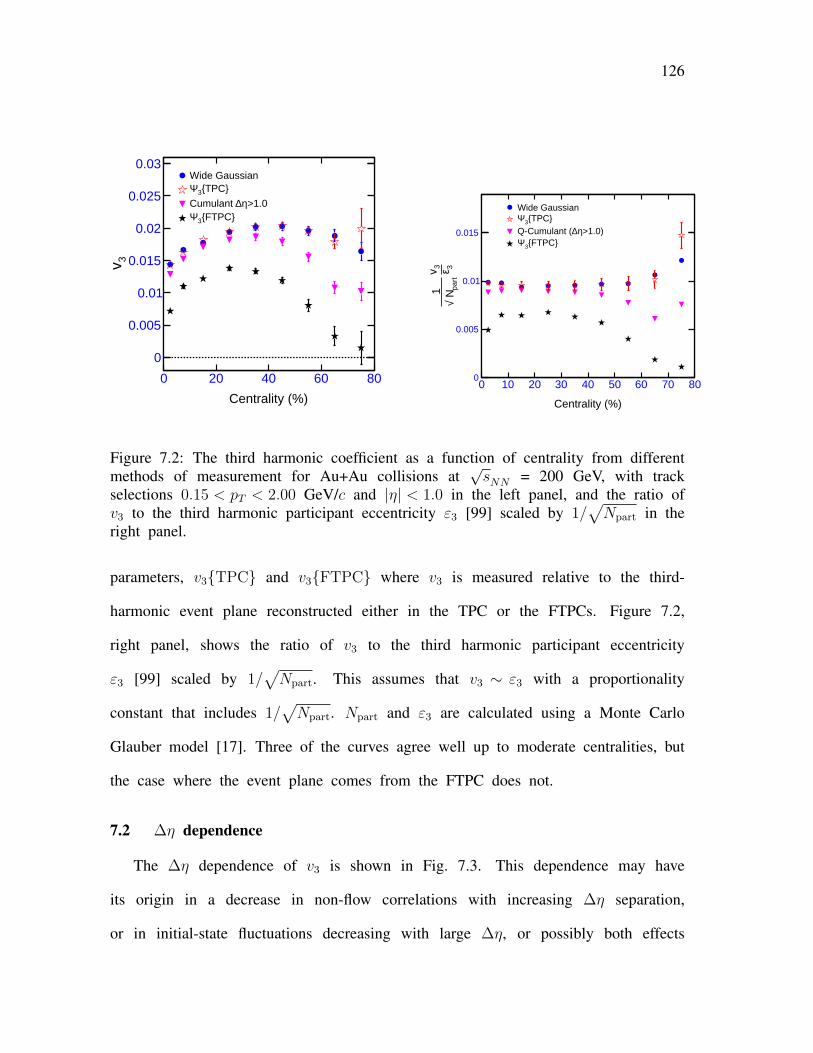
126

Centrality (%)

0 20 40 60 80

3v

0

0.005

0.01

0.015

0.02

0.025

0.03Wide Gaussian

{TPC}3Ψ>1.0 η∆Cumulant

{FTPC}3Ψ

Centrality (%)

0 10 20 30 40 50 60 70 80

3ε3v pa

rt N√1

0

0.005

0.01

0.015

Wide Gaussian {TPC}3Ψ

>1.0) η∆Q-Cumulant ({FTPC}3Ψ

Figure 7.2: The third harmonic coefficient as a function of centrality from differentmethods of measurement for Au+Au collisions at

√sNN = 200 GeV, with track

selections 0.15 < pT < 2.00 GeV/c and |η| < 1.0 in the left panel, and the ratio ofv3 to the third harmonic participant eccentricity ε3 [99] scaled by 1/

√Npart in the

right panel.

parameters, v3{TPC} and v3{FTPC} where v3 is measured relative to the third-

harmonic event plane reconstructed either in the TPC or the FTPCs. Figure 7.2,

right panel, shows the ratio of v3 to the third harmonic participant eccentricity

ε3 [99] scaled by 1/√Npart. This assumes that v3 ∼ ε3 with a proportionality

constant that includes 1/√Npart. Npart and ε3 are calculated using a Monte Carlo

Glauber model [17]. Three of the curves agree well up to moderate centralities, but

the case where the event plane comes from the FTPC does not.

7.2 ∆η dependence

The ∆η dependence of v3 is shown in Fig. 7.3. This dependence may have

its origin in a decrease in non-flow correlations with increasing ∆η separation,

or in initial-state fluctuations decreasing with large ∆η, or possibly both effects

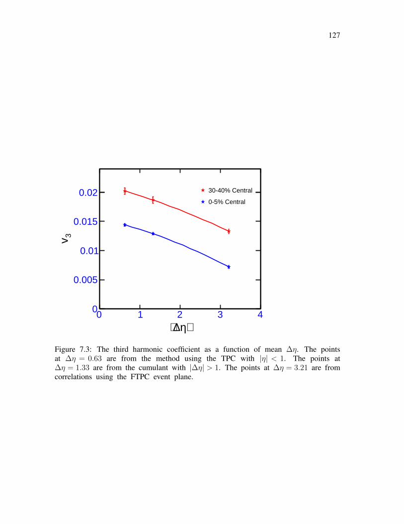
127

⟩η∆⟨0 1 2 3 4

3v

0

0.005

0.01

0.015

0.02 30-40% Central

0-5% Central

Figure 7.3: The third harmonic coefficient as a function of mean ∆η. The pointsat ∆η = 0.63 are from the method using the TPC with |η| < 1. The points at∆η = 1.33 are from the cumulant with |∆η| > 1. The points at ∆η = 3.21 are fromcorrelations using the FTPC event plane.

128

may contribute. If v23{2} is related to the initial eccentricity fluctuations, then

the reduction of v23{2} at large ∆η would presumably require a decrease of the

initial-state fluctuations at large rapidity separations. Recent work has found such a

decoherence effect with a hadron and parton cascade model [106]. Thus it is not

clear if one should extrapolate to large ∆η to avoid non-flow, or to small ∆η to

measure all the fluctuations [106]. More theoretical input is necessary to advance

our understanding of the ∆η dependence of this signal.

7.3 η and pT dependence

Figure 7.4 shows the η dependence of v3 using event plane methods. For

particles in the TPC using the η sub-event method, v3 is somewhat peaked at

mid-rapidity in peripheral collisions. With the event plane in the FTPCs, there is a

large η gap and v3 is flat at all centralities. This suggests that acceptance effects

at the edges of the TPC are not important. Thus, even though a large ∆η means

that one of the particles is probably at large η, this evidently does not have a large

effect on the η dependence of the signal. Figure 7.5 shows the third harmonic

coefficient as a function of pT at different centralities for AuAu collisions at√sNN=

200 GeV, measured with respect to the event planes constructed either in the TPC

or FTPCs. The average ∆η is 0.63 using the TPC event plane, and is 3.21 using

the FTPC event plane. The difference between the two methods can be understood

in terms of a ∆η dependence of the signal.

7.4 Comparisons with other experiments

In Fig. 7.6, it is evident that STAR v3 results with the event plane from the

TPC are very similar to those of PHENIX [101]. This is surprising, because the

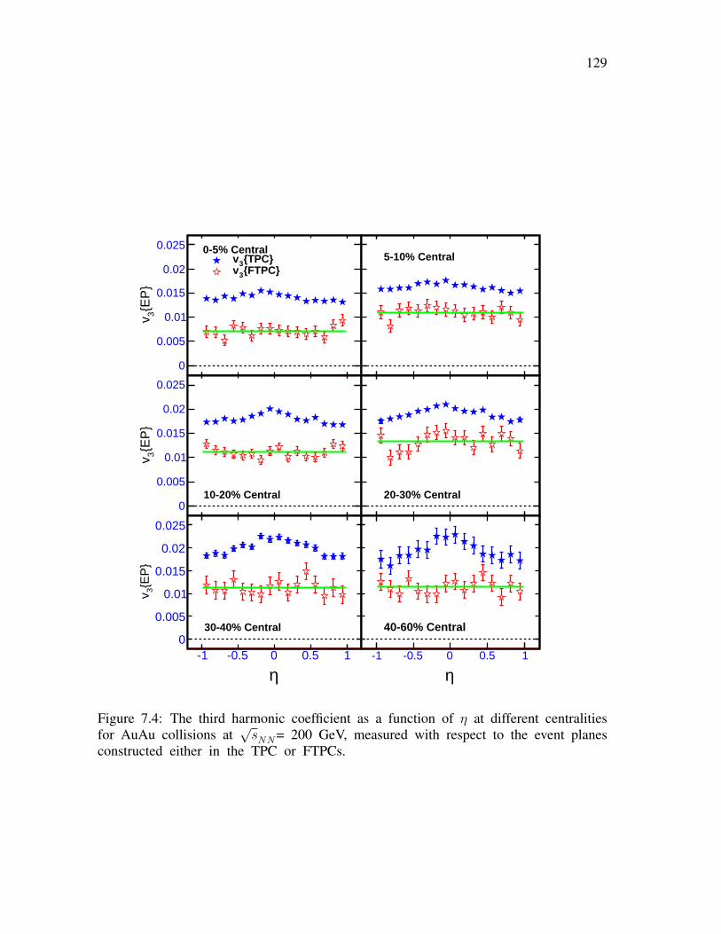
129

η-1 -0.5 0 0.5 1

{EP

}3v

0

0.005

0.01

0.015

0.02

0.025 0-5% Central{TPC}3v{FTPC}3v

η-1 -0.5 0 0.5 1

{EP

}3v

0

0.005

0.01

0.015

0.02

0.025

10-20% Central

η-1 -0.5 0 0.5 1

{EP

}3v

0

0.005

0.01

0.015

0.02

0.025

30-40% Central

η-1 -0.5 0 0.5 1

{EP

}3v

0

0.005

0.01

0.015

0.02

0.0255-10% Central

η-1 -0.5 0 0.5 1

{EP

}3v

0

0.005

0.01

0.015

0.02

0.025

20-30% Central

η-1 -0.5 0 0.5 1

{EP

}3v

0

0.005

0.01

0.015

0.02

0.025

40-60% Central

Figure 7.4: The third harmonic coefficient as a function of η at different centralitiesfor AuAu collisions at

√sNN= 200 GeV, measured with respect to the event planes

constructed either in the TPC or FTPCs.

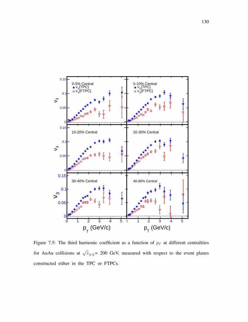
130

(GeV/c)T

p0 1 2 3 4 5

3v

0

0.05

0.1

0.15

0-5% Central{TPC}3v{FTPC}3v

(GeV/c)T

p0 1 2 3 4 5

3v

0

0.05

0.1

0.15

10-20% Central

(GeV/c)T

p0 1 2 3 4 5

3v

0

0.05

0.1

0.1530-40% Central

(GeV/c)T

p0 1 2 3 4 5

3v0

0.05

0.1

0.15

5-10% Central{TPC}3v{FTPC}3v

(GeV/c)T

p0 1 2 3 4 5

3v

0

0.05

0.1

0.15

20-30% Central

(GeV/c)T

p0 1 2 3 4 5

3v

0

0.05

0.1

0.1540-60% Central

Figure 7.5: The third harmonic coefficient as a function of pT at different centralities

for AuAu collisions at√sNN= 200 GeV, measured with respect to the event planes

constructed either in the TPC or FTPCs.

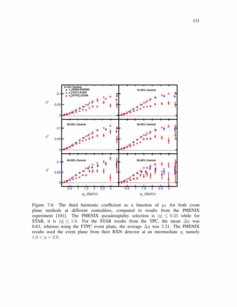
131

0.5 1 1.5 2 2.5 3

3v

0

0.05

0.1

010% Central:PHENIX{RXN}

3v

:STAR{TPC}3

v:STAR{FTPC}

3v

0.5 1 1.5 2 2.5 3

3v

0

0.05

0.1

2030% Central

(GeV/c)T

p

0.5 1 1.5 2 2.5 3

3v

0

0.05

0.14050% Central

0.5 1 1.5 2 2.5 3

0

0.05

0.1

1020% Central

0.5 1 1.5 2 2.5 3

0

0.05

0.1

3040% Central

(GeV/c)T

p

0.5 1 1.5 2 2.5 3

0

0.05

0.15060% Central

Figure 7.6: The third harmonic coefficient as a function of pT for both eventplane methods at different centralities, compared to results from the PHENIXexperiment [101]. The PHENIX pseudorapidity selection is |η| ≤ 0.35 while forSTAR, it is |η| ≤ 1.0. For the STAR results from the TPC, the mean ∆η was0.63, whereas using the FTPC event plane, the average ∆η was 3.21. The PHENIXresults used the event plane from their RXN detector at an intermediate η, namely1.0 < η < 2.8.

132

mean η of their RXN detector is larger than the same for sub-events in the STAR

TPC. Our FTPC results are lower than the PHENIX v3 measurements. This is

expected, because the mean ∆η is considerably larger in the STAR FTPC than in

the PHENIX RXN detector.

7.5 Model Comparisons

Event-by-event ideal hydro calculations of v3 have been reported by Qiu and

Heinz [103]. These authors concluded that instead of averaged initial conditions,

event-by-event calculations are necessary to compare with experimental data. The

first prediction of v3 with viscous hydro was in Ref. [46]. In Fig. 7.7, v2 and v3

as a function of transverse momentum are compared with several models for 0–5%

and 30–40% central collisions. The specific models are the viscous hydrodynamic

model of Ref. [45], where the ratio of viscosity to entropy is η/S = 0.08 and

0.16, and the AMPT model [?]. Predictions of v3 from the Parton-Hadron-String

Dynamics model [105] at 30–40% centrality for |η| < 0.5 have been reported using

the sub-event method with the event planes at 1.0 < |η| < 4.0, and are also plotted

in Fig. 7.7, at the lower right.

Elliptic flow results are mostly described by ideal hydrodynamics in the case of

the most central collisions, and by η/S = 0.08 in the case of mid-central collisions.

We find that the third harmonic coefficient results are also described by the same

model with similar viscosities. The PHSD model [105] also agrees with data.

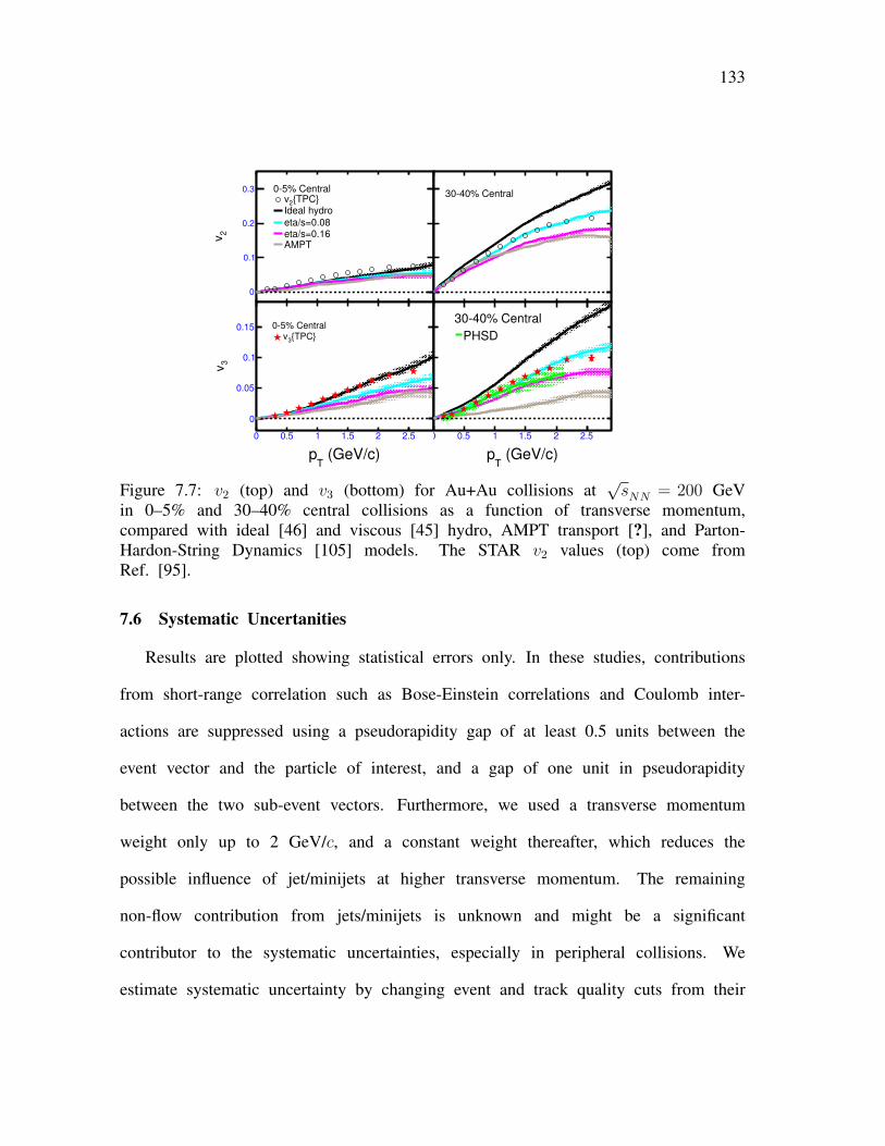
133

0 0.5 1 1.5 2 2.5

2v

0

0.1

0.2

0.3 05% Central{TPC}2v

Ideal hydro

eta/s=0.08eta/s=0.16AMPT

(GeV/c)T

p

0 0.5 1 1.5 2 2.5

3v

0

0.05

0.1

0.15 05% Central{TPC}3v

0 0.5 1 1.5 2 2.5

0

0.1

0.2

0.33040% Central

(GeV/c)T

p

0 0.5 1 1.5 2 2.5

0

0.05

0.1

0.153040% Central

PHSD

Figure 7.7: v2 (top) and v3 (bottom) for Au+Au collisions at√sNN = 200 GeV

in 0–5% and 30–40% central collisions as a function of transverse momentum,compared with ideal [46] and viscous [45] hydro, AMPT transport [?], and Parton-Hardon-String Dynamics [105] models. The STAR v2 values (top) come fromRef. [95].

7.6 Systematic Uncertanities

Results are plotted showing statistical errors only. In these studies, contributions

from short-range correlation such as Bose-Einstein correlations and Coulomb inter-

actions are suppressed using a pseudorapidity gap of at least 0.5 units between the

event vector and the particle of interest, and a gap of one unit in pseudorapidity

between the two sub-event vectors. Furthermore, we used a transverse momentum

weight only up to 2 GeV/c, and a constant weight thereafter, which reduces the

possible influence of jet/minijets at higher transverse momentum. The remaining

non-flow contribution from jets/minijets is unknown and might be a significant

contributor to the systematic uncertainties, especially in peripheral collisions. We

estimate systematic uncertainty by changing event and track quality cuts from their

134

central values. The total systematic uncertainty is evaluated by adding the uncer-

tainties measured in different cases in quadrature. Based on the factors mentioned

above, the resulting error estimate is about 10%, but this does not include the

unknown jet/minijet contribution.

7.7 Summary

I presented measurements of triangular flow of charged particles from Au+Au

collisions at√sNN = 200 GeV as a function of pseudorapidity, transverse momentum,

and centrality. Short-range correlations are eliminated by an η gap or by eliminating

the narrow Gaussian in pseudorapidity separation. Results are reported based on a

two-particle method for particle pairs, fitted with a wide Gaussian in pseudorapidity

separation, as well as from the standard event-plane method at mid-rapidity or at

forward rapidity. The measured values of v3 continuously decrease as mean ∆η

increases. It is not know whether this decrease is due to a decrease in non-flow

correlations or a decrease in fluctuations.

It is observed that v3 increases with transverse momentum before it levels-off

between 2 and 3 GeV/c, similar to the case of elliptic flow. We observe that the

ratio of v3 to ε3 is almost linear, except for the case when the event plane is

derived from the FTPCs. This observation supports the view that v3 originates from

initial-state density fluctuations. Our results are mostly described by hydrodynamic

models with small viscosity.

Chapter 8

RESULTS – IV: DIPOLE ASYMMETRY

In this chapter, I present measurements of azimuthal anisotropy at mid-rapidity

originating from dipole asymmetry in AuAu collisions at√sNN = 200 GeV. With

this type of observable, conventional rapidity odd directed flow is suppressed and

momentum conservation effect is corrected, leaving only a correlation which can

be attributed to fluctuations in the initial geometry. This measurement is a first-

harmonic flow coefficient, and is reported as a function of pseudorapidity and

transverse momentum for different centralities. The dataset under investigation

comes from run IV (from the year 2004). This is the first measurement of this

new observable at RHIC, and it provides an additional way to study initial-state

fluctuations, and the subsequent evolution of the collision system [43].

8.1 Pseudorapidity Dependence

Figure. 8.1 presents the first flow harmonic associated with dipole asymmetry in

AuAu collisions at√sNN = 200 GeV as a function of η. Each panel corresponds

to a different centrality, ranging from 0–5% through 70–80%. As explained in

Ref. [44], not much η dependence is expected, which our measurements confirm

for central collisions. However, in more peripheral collisions, much increased η

dependence is observed, which might be a viscous effect and/or may arise from

non-flow correlations. We are not aware of any pertinent model calculations, and

future theoretical study may shed light on it.

135

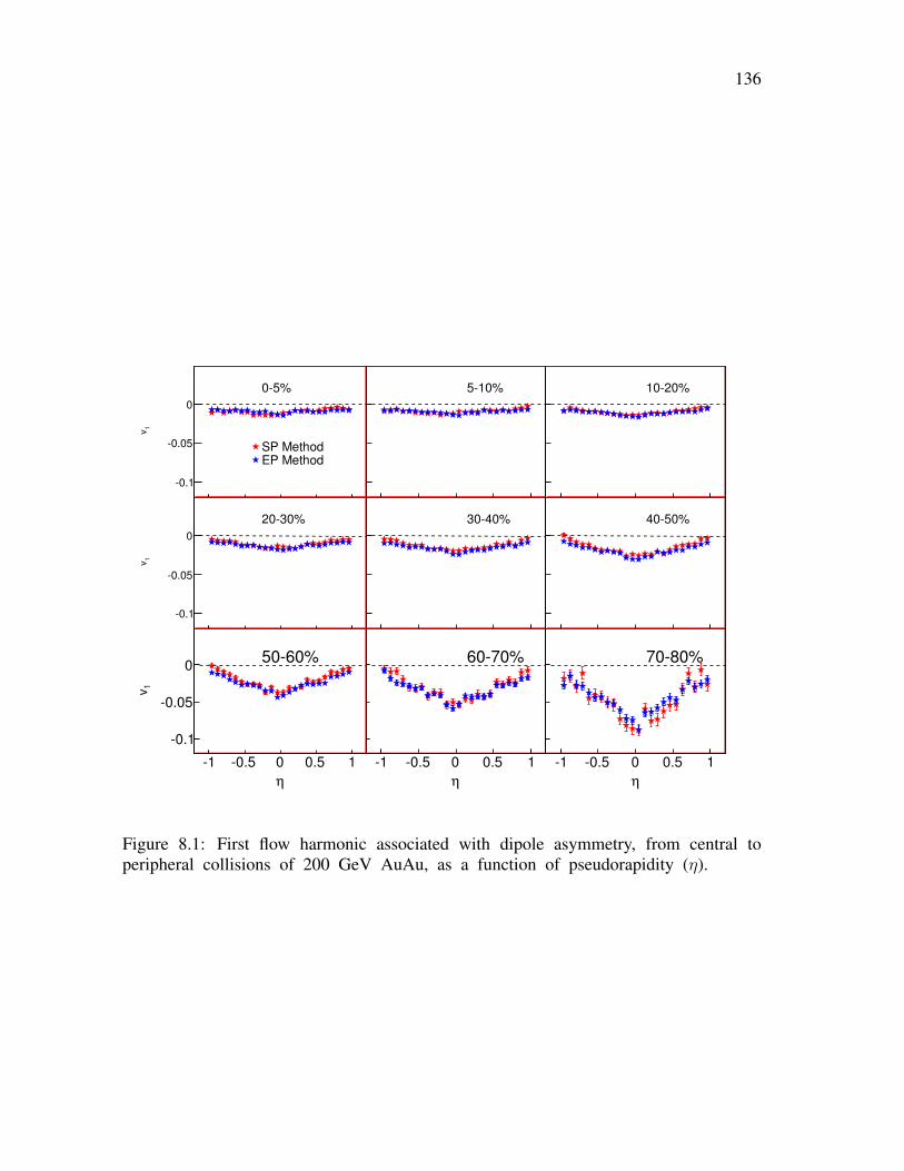
136

1 0.5 0 0.5 1

1v

0.1

0.05

0

05%

SP Method

EP Method

1 0.5 0 0.5 1

1v

0.1

0.05

0

2030%

η

1 0.5 0 0.5 1

1v

0.1

0.05

05060%

1 0.5 0 0.5 1

0.1

0.05

0

510%

1 0.5 0 0.5 1

0.1

0.05

0

3040%

η

1 0.5 0 0.5 1

0.1

0.05

06070%

1 0.5 0 0.5 1

0.1

0.05

0

1020%

1 0.5 0 0.5 1

0.1

0.05

0

4050%

η

1 0.5 0 0.5 1

0.1

0.05

07080%

Figure 8.1: First flow harmonic associated with dipole asymmetry, from central toperipheral collisions of 200 GeV AuAu, as a function of pseudorapidity (η).

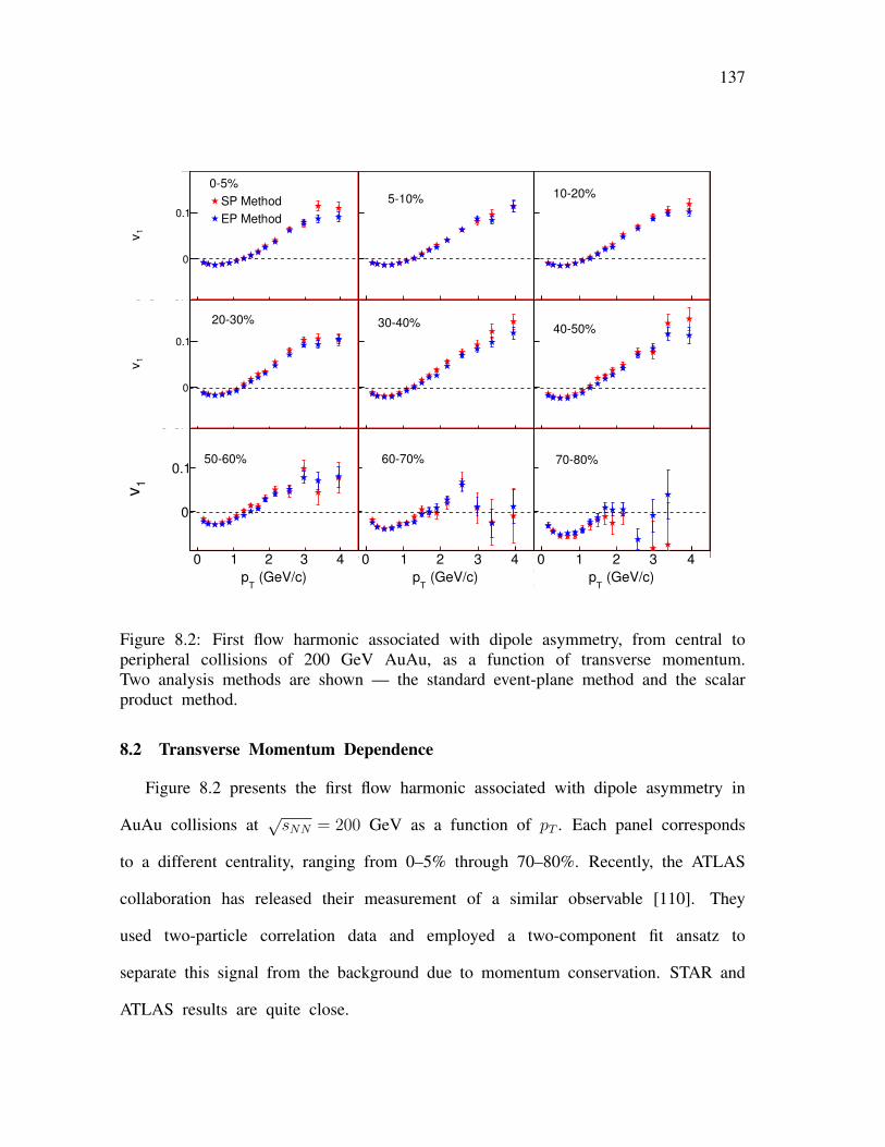
137

0 1 2 3 4

0

0.1 0 1 2 3 4

1v

0

0.1

05%

SP Method

EP Method

0 1 2 3 4

1v

0

0.1

2030%

(GeV/c)T

p

0 1 2 3 4

1v

0

0.15060%

0 1 2 3 4

0

0.1

510%

0 1 2 3 4

0

0.1

3040%

(GeV/c)T

p

0 1 2 3 4

0

0.16070%

0 1 2 3 4

0

0.1

1020%

0 1 2 3 4

0

0.14050%

(GeV/c)T

p

0 1 2 3 4

0

0.17080%

Figure 8.2: First flow harmonic associated with dipole asymmetry, from central toperipheral collisions of 200 GeV AuAu, as a function of transverse momentum.Two analysis methods are shown — the standard event-plane method and the scalarproduct method.

8.2 Transverse Momentum Dependence

Figure 8.2 presents the first flow harmonic associated with dipole asymmetry in

AuAu collisions at√sNN = 200 GeV as a function of pT . Each panel corresponds

to a different centrality, ranging from 0–5% through 70–80%. Recently, the ATLAS

collaboration has released their measurement of a similar observable [110]. They

used two-particle correlation data and employed a two-component fit ansatz to

separate this signal from the background due to momentum conservation. STAR and

ATLAS results are quite close.

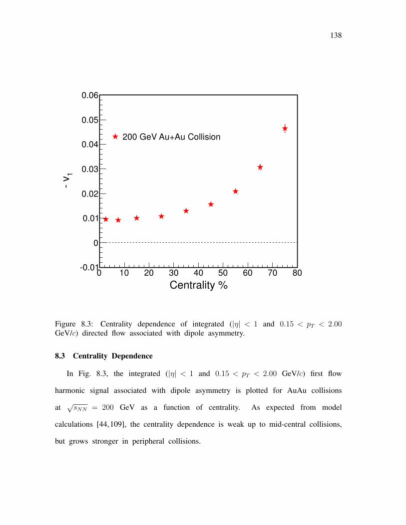
138

Centrality %

0 10 20 30 40 50 60 70 80

1

v

0.01

0

0.01

0.02

0.03

0.04

0.05

0.06

200 GeV Au+Au Collision

Figure 8.3: Centrality dependence of integrated (|η| < 1 and 0.15 < pT < 2.00GeV/c) directed flow associated with dipole asymmetry.

8.3 Centrality Dependence

In Fig. 8.3, the integrated (|η| < 1 and 0.15 < pT < 2.00 GeV/c) first flow

harmonic signal associated with dipole asymmetry is plotted for AuAu collisions

at√sNN = 200 GeV as a function of centrality. As expected from model

calculations [44,109], the centrality dependence is weak up to mid-central collisions,

but grows stronger in peripheral collisions.

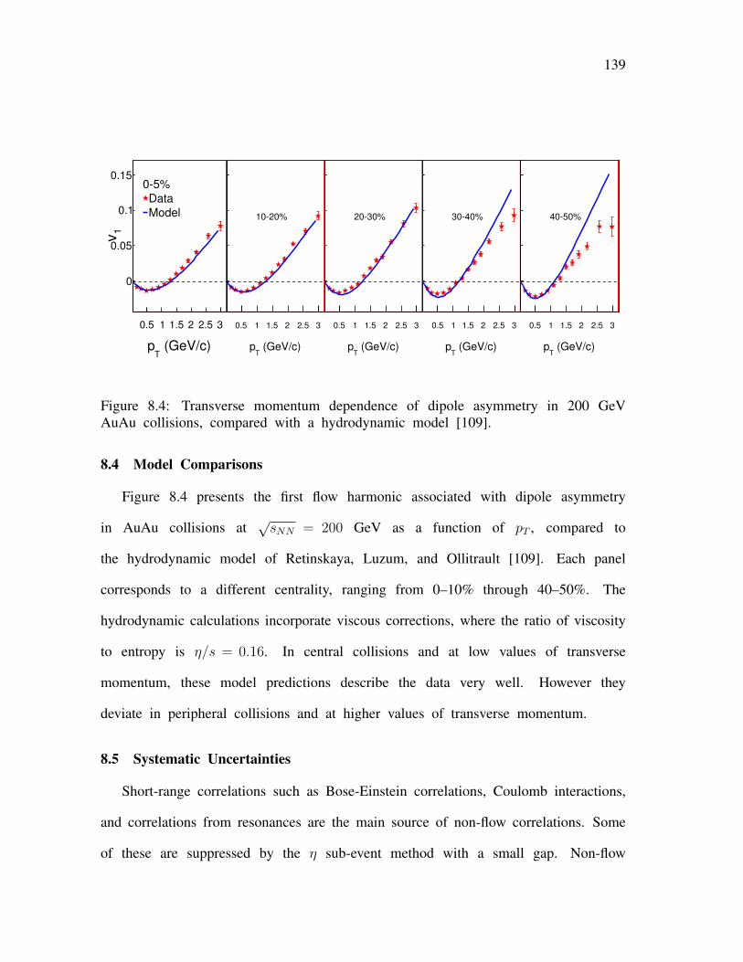
139

(GeV/c)T

p

0.5 1 1.5 2 2.5 3

1v

0

0.05

0.1

0.1505%

Data

Model

(GeV/c)T

p

0.5 1 1.5 2 2.5 3

0

0.05

0.1

0.15

1020%

(GeV/c)T

p

0.5 1 1.5 2 2.5 3

0

0.05

0.1

0.15

2030%

(GeV/c)T

p

0.5 1 1.5 2 2.5 3

0

0.05

0.1

0.15

3040%

(GeV/c)T

p

0.5 1 1.5 2 2.5 3

0

0.05

0.1

0.15

4050%

Figure 8.4: Transverse momentum dependence of dipole asymmetry in 200 GeVAuAu collisions, compared with a hydrodynamic model [109].

8.4 Model Comparisons

Figure 8.4 presents the first flow harmonic associated with dipole asymmetry

in AuAu collisions at√sNN = 200 GeV as a function of pT , compared to

the hydrodynamic model of Retinskaya, Luzum, and Ollitrault [109]. Each panel

corresponds to a different centrality, ranging from 0–10% through 40–50%. The

hydrodynamic calculations incorporate viscous corrections, where the ratio of viscosity

to entropy is η/s = 0.16. In central collisions and at low values of transverse

momentum, these model predictions describe the data very well. However they

deviate in peripheral collisions and at higher values of transverse momentum.


Short-range correlations such as Bose-Einstein correlations, Coulomb interactions,

and correlations from resonances are the main source of non-flow correlations. Some

of these are suppressed by the η sub-event method with a small gap. Non-flow

140

originating from jets/minijets [111] cannot be estimated. We use a constant weighting

factor of 2 GeV/c for all particles with pT > 2 GeV/c, which reduces the possible

influence from high transverse momentum jets/minijets. We estimate the systematic

uncertainty by means of changing event and track quality cuts from the optimal

values. The total systematic uncertainty is evaluated by adding the uncertainties from

the different sources in quadrature, which leads to an estimated overall systematic

error of about 10%.

8.6 Summary

The first measurements of the first harmonic coefficient associated with dipole

asymmetry in Au + Au collisions at√sNN = 200 GeV are presented. Results

are reported using the the standard event-plane method and the scalar product

method, with the flow vectors reconstructed with a pseudorapidity gap of 0.1 units

between the sub-event vectors, and at least 0.05 units of pseudorapidity between

the flow vector and the particle of interest. Results from both methods are

consistent with each other. It is observed that the centrality dependence of this

flow is weak up to mid-central collisions, and there is a large change in centrality

dependence thereafter, which may come from non-flow or from imperfect correction

for the unwanted correlation from momentum conservation. Recently, the ATLAS

collaboration has released their dipole asymmetry measurement at LHC energy.

They used two-particle correlation data and employed a two-component fit ansatz

to separate the pseudorapidity-even first harmonic coefficient from the signal due to

momentum conservation. The results presented here are quite similar to the ATLAS

results, and are mostly described by hydrodynamic models with a small viscosity for

central collisions, however, the models deviate from the data in peripheral collisions

141

at higher values of transverse momentum.

Chapter 9

SUMMARY AND CONCLUSIONS

Anisotropic flow sheds light on the early stage in high-energy heavy-ion collisions.

To minimize various systematic effects, especially the correlations that in practice

set a limit on how accurately flow can be measured, we have used a detector

subsystem called Beam Beam Counters (BBC) and developed a new method to

reconstruct the reaction plane from the energy deposition of the charged particles

collected by the BBC. This work focuses on the contribution of the BBC to the

estimation of the first-order event plane used in anisotropic flow analysis at Beam

Energy Scan (BES) energies (√sNN = 7.7, 11.5, 19.6, 27 and 39 GeV). This new

method vn{BBC} has proven itself to be reliable as evidenced by the agreement

with other independent methods, and is useful to suppress non-flow, because of the

large pseudorapidity gap between the BBCs and the central TPC. The first-order

event plane resolution is a quality factor such that unity represents a perfect reaction

plane determination. The event plane resolution is calculated by correlating east and

west BBC event planes. This resolution has a centrality dependence which reaches

a maximum around mid-central collisions, and also has a beam energy dependence

which decreases with increasing beam energy.

In the directed flow analysis, I studied all charged particles as well as identified

pions (±), kaons (±), protons and antiprotons in 7.7, 11.5, 19.6, 27 and 39 GeV

AuAu collisions. For CuCu collisions at 22.4 GeV and AuAu collisions at 9.2 GeV,

I studied directed flow for charged particles. Because of limited statistics, I was

142

143

not able to study identified particle flow at 22.4 and 9.2 GeV. I studied the flow

of charged particles in the pseudorapidity region covered by the STAR TPC and

FTPCs (up to η = 4.2) and for identified charged particles in the pseudorapidity

region covered by the STAR TPC.

I observed that charged particle v1 approaches zero close to the spectator

rapidities. This is an unremarkable effect predicted by all models, and can be

understood in terms of a change in the relative abundances of protons and pions at

forward pseudorapidities, where proton v1 and pion v1 likely have opposite signs,

but neither might have a wiggle shape. The rapidity dependence of v1 provides

further support for the limiting fragmentation picture in AuAu collisions as well as

in CuCu collisions.

Directed flow of identified particles is reported. Differences in directed flow are

observed between between positive and negative hadrons, and especially between

protons and antiprotons. This difference becomes smaller for higher beam energies.

For mid-central collisions, the proton v1 slope in the mid-rapidity region changes

sign from positive to negative between 7.7 and 11.5 GeV and remains small but

negative up to 200 GeV, while the slope for pions, kaons and antiprotons and

remains always negative. Based on transport model comparisons, the observed trends

in these data above 11.5 GeV can qualitatively be understood in terms of anisotropic

emission of produced particles from a tilted disk. A striking observation is that

the v1 slope for net protons, which is an estimate of the directed flow contribution

from initial-state baryon number transported to the midrapidity region, changes sign

twice within the energy range 7.7–39 GeV studied here. This result is qualitatively

different from the UrQMD transport model, which exhibits a monotonic trend with

144

no sign reversal, and has the potential to be the most unexpected and far-reaching

finding to emerge from this dissertation project. It is also noteworthy that a three-

fluid hydrodynamic model with a first-order phase transition [89] predicts a double

sign change that is qualitatively very similar to the STAR measurement. However,

the ultimate implication of this observation will most likely not be understood until

theoretical study with a specific focus on this signal has been completed, as well

as a new experimental study with higher statistics required for a measurement as a

function of centrality.

I measured the elliptic flow, v2, in AuAu collisions at√sNN = 7.7, 11.5, 19.6,

27 and 39 GeV for charged hadrons at mid-rapidity with respect to the first-order

event plane reconstructed at larger rapidity. This method is effective in suppressing

non-flow and flow fluctuation effects. The results from this method are consistent

with the v2{4} method. Comparing these results to the other measurement methods

like v2{TPC} and the two-particle cumulant v2{2} methods which are commonly

used in elliptic flow analysis, one can estimate the systematic uncertainties from

non-flow effects and flow fluctuations. The centrality, η and pT dependence of v2

are similar to those observed at higher RHIC beam energies. The integrated v2

signal increases from central to mid-central collisions, and it decreases in peripheral

collisions. The comparison with Au+Au collisions at higher RHIC energies (√sNN

= 62.4 and 200 GeV) and at LHC (PbPb collisions at√sNN = 2.76 TeV) shows

that the v2 values increase with increasing beam energy at low pT (pT < 2.0 GeV/c)

where hydrodymanic calculations are applicable.

Measurements of the elliptic flow for 22.4 GeV CuCu collisions are also

presented. We compare pT -integrated v2 with measurements at higher energies. The

145

pT -dependence of the measured v2 at 22.4 GeV is similar to that at 62.4 and 200

GeV. UrQMD and AMPT models (the latter both with and without string melting)

do not agree with the present measurements.

In triangular flow analysis, I concentrated on AuAu collisions at√sNN = 200

GeV from the year 2004 (run 4). I present measurements of triangular flow

of charged particles as a function of pseudorapidity, transverse momentum, and

centrality. I report result from a two-particle method for particle pairs fit with a

wide Gaussian in pseudorapidity separation, as well as from the standard event-

plane method at mid-rapidity or at forward rapidity. The measured values of v3

continuously decrease as mean ∆η increases. It is not known whether this decrease

is due to a decrease in non-flow correlations or a decrease in fluctuations. We

observe that v3 increases with transverse momentum before it levels-off between 2

and 3 GeV/c, similar to the case of elliptic flow. Our results are mostly described

by hydrodynamic models with small viscosity. It is observed that the ratio of v3 to

ε3 is almost linear, except for the case with the event plane in the FTPCs. This

observation supports the view that v3 originates from initial-state density fluctuations.

I presented the first measurements of the first harmonic coefficient associated

with dipole asymmetry from AuAu collisions at√sNN = 200 GeV. I report results

from the standard event plane method and the scalar product method, with the flow

vectors reconstructed with a pseudorapidity gap of 0.1 units between the sub-event

vectors, and at least 0.05 units of pseudorapidity between the flow vector and the

particle of interest. Results from both methods are consistent with each other. It

is observed that the centrality dependence of this flow is weak up to mid-central

collisions, and there is a large change in centrality dependence thereafter, which may

146

come from non-flow or non-perfect correction for momentum conservation. These

results are mostly described by hydrodynamic models with a small viscosity for

central collisions. However, the models deviate from the data in peripheral collisions

at higher transverse momentum. Measurements related to initial density fluctuations

are a new area of physics analysis in STAR, and they help us to understand the

collision dynamics.

There is general agreement in the heavy-ion collision community that a new

form of matter is being produced at the top RHIC energy, and that it has many

of the characteristics expected of a strongly-interacting Quark-Gluon Plasma (sQGP).

We are now in the follow-on stage of studying the properties of this new phase

of matter, and STAR has now progressed to the stage of mapping the evolution of

these properties with beam energy. During the beam energy scan program at RHIC,

we are looking for the disappearance of the QGP signatures observed at top RHIC

energy. We also are searching for signatures of the hypothesized critical point and

first-order phase boundary. The RHIC energy scan program is in its first phase. I

have presented some interesting experimental observations and new theoretical input

is necessary to fully understand these observations. Elliptic flow study with respect

to the first-order event plane certainly helps to disentangle the flow from non-flow

and flow fluctuations. We are now just beginning to study triangular flow and first

flow harmonics due to dipole asymmetry at RHIC, one of the main topics of this

dissertation. Therefore, we emphasize that it is too early to expect this work to have

well-understood consequences for the “big picture” at RHIC, and in the meantime,

I make the argument that the analyses in this dissertation have strongly challenged

the theoretical community, especially in the area of directed flow for transported

147

baryon number. Moreover, this work has paved the way for the next rounds of

experimental analyses.

Bibliography

[1] Quark-Gluon Plasma 3, edited by R. C. Hwa and X. N. Wang, WorldScientific, Singapore (2003).

[2] Introduction to High-Energy Heavy-Ion Collisions, C.-Y. Wong, World Scien-tific, Singapore (1994).

[3] For recent developments, see Proceedings of Quark Matter 2011, Annecy,France, J. of Phys. G 38 (2011).

[4] K. Geiger, Phys. Rev. D 46, 4965 (1992).

[5] Y. Aoki et al., Nature 443, 675 (2006); Y. Aoki et al., Phys. Lett. B 46,643 (2006); M. Cheng et al., Phys. Rev. D 74, 054507 (2006).

[6] F. R. Brown et al., Phys. Rev. Lett. 65, 2491 (1990); A. Bazavov et al.(HotQCD Collaboration), Phys. Rev. D 80, 014504 (2009); S. Borsanyi et al.(Wuppertal-Budapest Collaboration), J. High Energy Phys. 11, 077 (2010).

[7] S. Ejiri, Phys. Rev. D 78, 074507 (2008); E. S. Bowman, J. I. Kapusta, Phys.Rev. C 79, 015202 (2009); Y. Hatta and T. Ikeda, Phys. Rev. D 67, 014028(2003).

[8] B. I. Abelev et al. (STAR Collaboration), arXiv:1007.2613.

[9] The Phenix Collaboration: http://www.phenix.bnl.gov .

[10] A. Aduszkiewicz, Acta Phys. Polonica B 43, 635 (2012).

[11] P. Staszel (for the CBM Collaboration), Acta Phys. Polonica B 41, 2 (2010).

[12] The NICA Collaboration: http://nica.jinr.ru .

[13] B. I. Abelev et al. (STAR Collaboration), Phys. Rev. C 81, 24911 (2010).

[14] A. M. Poskanzer and S. A. Voloshin, Phys. Rev. C 58, 1671 (1998).

[15] B. I. Abelev et al. (STAR Collaboration), Phys. Rev. Lett. 99, 112301 (2007);J. Adams et al. (STAR Collaboration), Phys. Rev. Lett 95, 122301 (2005).

[16] M. H. Thoma and M. Gyulassy, Nucl. Phys. A 538, 37c (1991); S. Mrowczyn-ski, Phys. Lett. B 269, 383 (1991); Y. Koike and T. Matsui, Phys. Rev. D45, 3237 (1992); M. Gyulassy and M. Plumer, Phys. Lett. B 243, 432 (1990).

148

149

[17] M. L. Miller, K. Reygers, S. J. Sanders and P. Steinberg, Ann. Rev. Nucl.Part. Sci. 57, 205 (2007); B. Alver et al., Phys. Rev. C 77, 014906 (2008).


[19] S. Gavin and G. Moschelli, Phys. Rev. C 85, 014905 (2012); A. Dumitru,F. Gelis, L. McLerran, and R. Venugopalan, Nucl Phys. A 810, 91 (2008);S. Gavin, L. McLerran, and G. Moschelli, Phys. Rev. C 79, 051902 (2009);G. Moschelli and S. Gavin, Nucl. Phys. A 836, 43 (2010); K. Dusling, D.Fernandez-Fraile, and R. Venugopalan, Nucl. Phys. A 828, 161 (2009).

[20] B. Alver and G. Roland, Phys. Rev. C 81, 054905 (2010).

[21] P. Sorensen, B. Bolliet, A. Mocsy, Y. Pandit and N. Pruthi, Phys. Lett. B705, 71 (2011).

[22] B. I. Abelev et al., Phys. Rev. Lett. 103, 251601 (2009).

[23] S. A. Voloshin, Phys. Rev. C 70, 057901 (2004).

[24] J. Brachmann, S. Soff, A. Dumitru, H. Stocker, J. A. Maruhn, W. Greiner,L. V. Bravina, and D. H. Rischke, Phys. Rev. C 61, 024909 (2000); L. P.Csernai and D. Roehrich, Phys. Lett. B 458, 454 (1999); M. Bleicher and H.Stocker, Phys. Lett. B 526, 309 (2002).

[25] T. Csorgo, PoS CPOD2009, 035 (2009) (arXiv:0911.5015v1 [nucl-th])

[26] C. Athanasiou, K. Rajagopal and M. Stephanov, Phys. Rev. D 82, 074008(2010).

[27] M. A. Stephanov, Phys. Rev. Lett. 102, 032301 (2009).

[28] J. Adams et al. ( STAR Collaboration), Phys. Rev. C 72, 044902 (2005).

[29] M. A. Stephanov, Phys. Rev. Lett. 102, 032301 (2009).

[30] X. F. Luo for the STAR Collaboration, J. Phys. Conf. Ser. 316, 012003(2011).

[31] R. Hanbury-Brown and R. Q. Twiss, Phil. Mag. 45, 663 (1954); S. E. Koonin,Phys. Lett. B 70, 43 (1977); F. B. Yano and S. E. Koonin, Phys. Lett. B 78,556 (1978); S. Pratt, Phys. Rev. Lett. 53, 1219 (1984); S. Pratt, Phys. Rev.D 33, 1314 (1986); U. Heinz, Nucl. Phys. A 610, 264c (1996).

[32] M. A. Lisa and S. Pratt, arXiv:0811.1352.

[33] N. Herrmann, J. P. Wessels, and T. Wienold, Annu. Rev. Nucl. Part. Sci. 49,581 (1999); M. Bleicher and H. Stocker, Phys. Lett. B 526, 309 (2002); J.Y. Chen et al., Phys. Rev. C 81, 014904 (2010).

150

[34] P. Huovinen in Quark-Gluon Plasma 3, Eds: R. C. Hwa, X. N. Wang (WorldScientific, Singapore, 2003), p. 616.

[35] J . Adams et al. (STAR Collaboration), Phys. Rev. Lett. 101, 252301 (2008).

[36] P. Bozek and I. Wyskiel, Phys. Rev. C 81, 054902 (2010).

[37] R. J. Snellings, H. Sorge, S. A. Voloshin, F. Q. Wang and N. Xu, Phys. Rev.Lett 84, 2803 (2000).

[38] G. Burau et al., Phys. Rev. C 71, 054905 (2005).

[39] STAR-TOF software documentation:http://drupal.star.bnl.gov/STAR/system/files/TOFSoftware.2.pdf.

[40] C. Alt et al. (NA49 Collaboration), Phys. Rev. C 68, 034903 (2003).

[41] Heiselberg and A.-M. Levy, Phys. Rev. C 59, 2716 (1999).

[42] A. Bialas, M. Bleszynski and W. Czyz, Nucl. Phys. B 111, 461 (1976).

[43] D. Teaney and L. Yan, Phys. Rev. C 83, 064904 (2011).

[44] M. Luzum and J. Y. Ollitrault, Phys. Rev. Lett. 106, 102301 (2011).

[45] B. Schenke, S. Y. Jeon, and C. Gale, Phys. Rev. Lett. 106, 042301 (2011).

[46] B. H. Alver, C. Gombeaud, M. Luzum and J. Y. Ollitrault, Phys. Rev. C 82,034913 (2010).

[47] J. Y. Ollitrault, A. M. Poskanzer, and S. A. Voloshin, Phys. Rev. C 80,014904 (2009).

[48] A. Adare et al. (PHENIX Collaboration), Phys. Rev. Lett. 107, 252301 (2011).

[49] B. Alver et al. (PHOBOS Collaboration), Phys. Rev. C 81, 034915 (2010).

[50] H. Sorge, H. Stocker, and W. Griener, Ann. Phys. 192, 266 (1989); H. Sorge,Phys. Lett. B 402, 251 (1997); Phys. Rev. Lett. 82, 2048 (1999).

[51] T. Maruyama et al., Prog. Theor. Phys. 96, 263 (1996).

[52] S. A. Bass et al., Prog. Part. Nucl. Phys. 41, 225 (1998); M. Bleicher et al.,J. Phys. G 25, 1859 (1999); L. A. Winckelmann et al., Nucl. Phys. A 610,116c (1996).

[53] Z. W. Lin and C.-M. Ko, Phys. Rev. C 65, 034904 (2002); L.-W. Chen,C.-M. Ko, J. Phys. G 31, S49 (2005).

151

[54] K. H. Ackermann et al. (STAR collaboration), Nucl. Instr. Meth. A 499, 624(2003).

[55] M. Anderson et al., Nucl. Instr. Meth. A 499, 659 (2003); K. H. Ackermannet al. (STAR collaboration), Nucl. Phys. A 661, 681c (1999).

[56] F. Bergsma et al., Nucl. Instr. Meth. A 499, 629 (2003).

[57] Y. Bar-Shalom, X. R. Li and T. Kirubarajan, Estimation With Applications toTracking and Navigation, John Wiley Sons (New York), 2001.

[58] K. H. Ackermann et al., Nucl. Instr. Meth. A 499, 713 (2003).

[59] C. A. Whitten, Jr. (for the STAR Collaboration), AIP Conf. Proc. 980, 390(2008).

[60] B. Bonner et al., Nucl. Instr. Meth. A 508, 181 (2003); W. J. Llope et al.,Nucl. Instr. Meth. A 522, 252 (2004); M. Shao et al., Nucl. Instr. Meth. A492, 344 (2002).

[61] Figures are obtained from the Brookhaven National Labora-tory Flickr web page under Creative Commons Attribution-Noncommercial-No Derivative Works 2.0 Generic License;http://www.flickr.com/photos/brookhavenlab/sets/72157613690851651/.

[62] A. Schmah, private communication.

[63] F. S. Bieser et al., Nucl. Instr. Meth. A 499, 766 (2003). C. Alder et al.,Nucl. Instr. Meth. A 470, 488 (2001). J. W. Harris et al., Nucl. Phys. A 566,277c (1994).

[64] B. Christie, S. White, P. Gorodetzky and D. Lazic, STAR Note SN0175,1994.

[65] D. Kharzeev and M. Nardi, Phys. Lett. B 507, 121 (2001).

[66] K. Nakamura et al. (Particle Data Group), J. Phys. G 37, 075021 (2010).

[67] B. B. Back et al. (PHOBOS Collaboration), Phys. Rev. C 70, 021902 (2004).


[69] The online monitoring of the BBC subsystem during data-taking is accessibleat http://online.star.bnl.gov/bbc/ .

[70] I. Selyuzhenkov and S. Voloshin, Phys. Rev. C 77, 034904 (2008).

[71] J. Barrette et al. (E877 Collaboration), Phys. Rev. C 55, 1420 (1997).

152

[72] P. Danielewicz, Phys. Rev. C 51, 716 (1995); J. Barrette et al. (E877Collaboration), Phys. Rev. C 55, 1420 (1997).

[73] J. Barrette et al. (E877 Collaboration), Phys. Rev. C 56, 3254 (1997).

[74] G. Agakishiev et al. (STAR Collaboration), Phys. Rev. C 85, 014901 (2012).

[75] A. Bilandzic, R. Snellings, and S. A. Voloshin, Phys. Rev. C 83, 044913(2011).

[76] A. Bilandzic, Ph.D. Dissertation, National Institute for Subatomic Physics(NIKHEF), Amsterdam, The Netherlands, 2011.

[77] C. Alder et al. (STAR Collaboration), Phys. Rev. C 66, 034904 (2002); N.Borghini, P. M. Dinh, and J. Y. Ollitrault, Phys. Rev. C 63, 054906 (2001).

[78] M. Anderson, P. M. Dinh, J. Y. Ollitrault, A. M. Poskanzer, and S. A.Voloshin, Phys. Rev. C 66, 014901 (2002).

[79] G. Wang, Ph.D. Dissertation, Kent State University, Kent, OH, 2006.

[80] Y. Pandit for the STAR Collaboration, J. Phys. Conf. Ser. 316, 012001 (2011).

[81] J. Brachmann et al., Phys. Rev. C 61, 024909 (2000).

[82] H. Sorge, Phys. Rev. Lett. 78, 2309 (1997).

[83] H. A. Gustafsson et al., Phys. Rev. Lett. 52, 1590 (1984).

[84] D. H. Rischke et al., Heavy Ion Phys. 1, 309 (1995).

[85] L. Adamczyk et al. (STAR Collaboration), Phys. Rev. Lett. 108, 202301(2012).

[86] Y. Pandit for the STAR Collaboration, Acta Phys. Pol. B, Proc. Supp. 5, 439(2012).

[87] L. P. Csernai and D. Rohrich, Phys. Lett. B 458, 45 (1999).

[88] L. V. Bravina et al., Phys. Lett. B 470, 27 (1999).

[89] H. Stocker, Nucl. Phys. A 750 121 (2005).

[90] J. Xu, L.-W. Chen, C. M. Ko, and Z. W. Lin, arXiv:1201.3391.

[91] B. B. Back et al. (PHOBOS Collaboration), Phys. Rev. Lett. 97, 012301(2006).

[92] S. A. Bass et al., Prog. Part. Nucl. Phys. 41, 255 (1998); M. Bleicher et al.,J. Phys. G 25, 1859 (1999).

153

[93] G. Agakishiev et al. (STAR Collaboration), BES v2 paper to be submitted.


[95] J. Adams et al. (STAR Collaboration), Phys. Rev. Lett. 95, 122301 (2005); J.Adams et al. (STAR Collaboration), Phys. Rev. C 72, 014904 (2005).

[96] K. Aamodt et al. (ALICE Collaboration), Phys. Rev. Lett. 107, 032301 (2011).

[97] B. I. Abelev et al. (the STAR Collaboration), Phys. Rev. C 75, 054906(2007).

[98] R. Nouicer for the PHOBOS Collaboration, J. Phys. G 34, 887 (2007).

[99] G. Y. Qin, H. Petersen, S. A. Bass, and B. Miller, Phys. Rev. C 82, 064903(2010).

[100] J. L. Nagle and M. P. McCumber, Phys. Rev. C 83, 044908 (2011).

[101] A. Adare et al. (PHENIX Collaboration), Phys. Rev. Lett. 107, 252301 (2011)[arXiv:1105.3928 [nucl-ex]].

[102] J. Xu and C. M. Ko, Phys. Rev. C 84 014903 (2011).

[103] Z. Qiu and U. W. Heinz, Phys. Rev. C 84, 024911 (2011) [arXiv:1104.0650[nucl-th]].

[104] M. R. Haque, M. Nasim and B. Mohanty, Phys. Rev. C 84, 067901 (2011)[arXiv:1111.5095 [nucl-ex]].

[105] V. P. Konchakovski, E. L. Bratkovskaya, W. Cassing, V. D. Toneev,S. A. Voloshin and V. Voronyuk, Phys. Rev. C 85, 044922 (2012)[arXiv:1201.3320 [nucl-th]].

[106] K. Dusling, F. Gelis, T. Lappi and R. Venugopalan, Nucl. Phys. A 836, 159(2010).

[107] H. Petersen, G.-Y. Qin, S. A. Bass, and B. Muller, Phys. Rev. C 82,041901(R) (2010).

[108] H. Petersen, C. Greiner, V. Bhattacharya and S. A. Bass, arXiv:1105.0340[nucl-th].

[109] E. Retinskaya, M. Luzum, and J. Y. Ollitrault, Phys. Rev. Lett. 108, 252302(2012).

[110] G. Aad et al. (ATLAS Collaboration), arXiv:1203.3087v2 [hep-ex].

[111] M. Daugherity for the STAR Collaboration, J. Phys. G 35, 104090 (2008);D. Kettler for the STAR Collaboration, PoS C ERP2010, 011 (2010); T. A.Trainor and D. T. Kettler, Phys. Rev. C 83, 034903 (2011).

Appendix A

AUTHOR’S CONTRIBUTION TO COLLABORATIVE RESEARCH

In addition to the physics analysis work described in this dissertation, I have

completed a number of “community service” tasks within the STAR collaboration,

i.e., tasks that are of benefit to part or all of the entire collaboration. I am one

of the proposers of using the STAR BBC as a reaction plane detector at lower

beam energies. I participated in the repair of the BBC hardware and during STAR

data-taking in 2010 and 2011, I worked as a STAR detector operator and BBC

expert. My BBC hardware work included monitoring the subsystem performance

and calibrating it.

In the area of community service software, I have worked on determining the

first-order event plane from BBC information. I developed software that uses the

hit pattern of charged particles in the BBC to open up multiple new physics

opportunities for other members of the STAR collaboration.

I am among the principal authors (PAs) of a paper devoted to 9.2 GeV AuAu

(this is a long paper published in Physical Review C), and my advisor and I are

the sole PAs of another paper on directed and elliptic flow at 22.4 GeV (also

published in Physical Review C). I am one of several PAs of a paper on elliptic

flow of charged particles at beam energies between 7–39 GeV, which has been

recently submitted for publication, and another jointly-led paper on triangular flow

at 200 GeV is almost ready for submission. Directed flow results at 7-39 GeV (a

paper based 100% on work in Chapter 5 of this dissertation) is now under review

154

155

in the Bulk Correlations Physics Working Group, and has been recommended by

STAR management as a suitable paper for submission to the prestigious physics-wide

journal Physical Review Letters. In my early studies, I carried out a simulation

study related to BBC event plane resolution using RQMD events. The result was

incorporated into a long STAR writeup now published in arXiv:1007.2613.

There are some additional data analysis projects which are still in a preliminary

stage, and have not been included in this dissertation. Measurement of a signal

related to possible local parity violation at lower beam energies, based on the first-

order BBC event plane, and a study of beam-energy and system-size dependence

of triangular flow are two such examples. Likewise, triangular flow results for

identified pions, kaons and protons in 200 GeV AuAu collisions are not included

in this dissertation.

I have presented invited talks or contributed presentations on this work at various

conferences and workshops. I presented at the RHIC and AGS Users Meeting, June

7-11, 2010, BNL, Upton NY, at the 27th Winter Workshop on Nuclear Dynamics,

Feb 6-13, 2011, Winter Park, Colorado, at the 11th International Conference on

Nucleus-Nucleus Collisions (NN2012), May 27- June 1, 2012, San Antonio, TX,

and at the premier conference in my field, Quark Matter 2011 (QM’11), and at

Strange Quark Matter (SQM 2011). Recently, my abstract on directed flow and

higher flow harmonics has been accepted for oral presentation in Quark Matter 2012

(August 2012 in Washington, DC). I am the sole listed author of the associated

paper in the proceedings of WWND 2011 and SQM 2011. I have also presented

a contributed short talk at the American Physical Society in 2010, and an invited

colloquium at the Central Department of Physics, Tribhuvan Univ., Kathmandu,

156

Nepal. A selected list of publications where I am among the principal authors for

papers and presentations can be found in Appendix B. STAR policy, following the

normal practice of large collaborations in High Energy and Nuclear Physics, lists

all authors on refereed publications strictly in alphabetical order.

Appendix B

PRESENTATIONS AND PUBLICATION

PRESENTATIONS

• Oral Presentation:

“Triangular Flow of Charged Particles in Heavy Ion Collisions from STAR

Experiment at RHIC” NN2012, May 27-June 1, 2012, San Antonio, Texas


“Directed Flow of Identified Charged Particles from the RHIC Beam Energy

Scan ” SQM2011, September 18-24, 2011, Karkow, Poland

• Poster :

“Triangular Flow of Identified Particles in Au +Au Collisions at√sNN = 200

GeV from the STAR Experiment ” RHIC AGS Users Meeting, June 20-24,

2011, Brookhaven National Lab, Upton, NY

• Poster:

“Directed Flow of Identified Particles in Au +Au Collisions at√sNN =

39,11.5 and 7.7 GeV from the STAR Experiment ” QM2011, March 13-18,

157

158

2011, Annecy, France

• Invited Talk :

“ Beam Energy Dependence of Directed and Elliptic Flow Results from STAR

experiment,” 27th Winter Workshop on Nuclear Dynamics, Feb 6-13, 2011

Winter Park, Colorado.


“ Directed and Elliptic Flow of Charged Hadrons in Cu+Cu collisions at√sNN = 22.4 GeV”, American Physical Society, 2010 Fall Meeting of the

APS Division of Nuclear Physics, November 2-6, 2010, Santa Fe, New Mexico

• Invited Talk :

“ Directed Flow Results from STAR Experiment,” RHIC and AGS Users

Meeting June 7-11, 2010, BNL, Upton NY

• Invited Talk :

“ Heavy Ion Collisions at RHIC, STAR Experiment and Kent State University”,

Central Department of Physics, TU, Kathmandu, March 19, 2010


“ Directed and Elliptic Flow of Charged Hadrons at√sNN = 22.4 GeV Cu+Cu

Collisions”, American Physical Society, APS April Meeting 2010, February

13-16, 2010, Washington DC.

159

SELECTED PUBLICATIONS

• “ STAR BBC as a Reaction Plane Detector at Low Beam Energies” Paper in

progress (to be submitted for Nucl. Instr. and Methods)

• “ Directed flow in Au+Au Collisions at√sNN = 7.7, 11.5, 19.6, 27 and 39

GeV ” Paper in progress (to be submitted for Physical Review Letters)

• “ Triangular Flow of Charged Particles in Au + Au Collisions at√sNN =

200 GeV ” Paper in Progress (to be submitted for Physical Review C)

• “ Inclusive Charged Hadron Elliptic Flow in Au + Au Collisions at√sNN =

7.7 - 39 GeV” Paper submitted for Physical Review C)

• “The Rise and Fall of the Ridge in Heavy Ion Collisions” Phys. Lett. B 705,

71(2011) (Paul Sorensen, Boris Bolliet, Agnes Mocsy, Yadav Pandit, Navneet

Pruthi)

• “ Directed and Elliptic Flow of Charged Particles in Cu+Cu Collisions at√sNN = 22.4 GeV” G. Agakishiev et al [STAR Collaboration], Phys. Rev.

C 85, 014901 (2012)

160

• “ Beam Energy Dependence of Directed and Elliptic Flow Measurement from

the STAR Experiment ” Yadav Pandit(for the STAR collaboration) 2011 J.

Phys.: Conf. Ser. 316 012001 [arXiv:1109.2799v1 [nucl-ex]]

• “ Identified Particle Production, Azimuthal Anisotropy, and Interferometry Mea-

surements in Au+Au Collisions at√sNN = 9.2 GeV,” B. I. Abelev et al[STAR

Collaboration] Phys. Rev. C 81, 024911 (2010) [arXiv:0909.4131 [nucl-ex]].

• “ An Experimental Exploration of the QCD Phase Diagram: The Search for

the Critical Point and the Onset of De-confinement,” M. M. Aggarwal et al.

[STAR Collaboration], arXiv:1007.2613 [nucl-ex].

Documents

Yadav Pandit, Ph.D., July 2012 NUCLEAR PHYSICS ... Pandit July 2012 Dissertation written by Yadav Pandit B. Sc., Tribhuvan University, Nepal, 1993 M. Sc., Tribhuvan University, Nepal,