Yaglom limitscan depend on the starting state

Ce travail conjoint avec Bob Foley1

est dedie a Francois Baccelli.

David McDonald2

Mathematics and StatisticsUniversity of Ottawa

david.r.mcdonald@gmail.com

12 January 2015

1Partially supported by NSF Grant CMMI-08564892Partially supported by NSERC Grant 4551 / 2011

A quotation

Semi-infinite random walk with absorption–Gambler’s ruin

Our example

Periodic Yaglom limits

Applying the theory

ρ-Martin entrance boundary

Closing words

The long run is a misleading guide . . .The long run is amisleading guide to currentaffairs. In the long run weare all dead. Economistsset themselves too easy,too useless a task if intempestuous seasons theycan only tell us that whenthe storm is past the oceanis flat again.

John Maynard Keynes

I Keynes was a Probabilist: Keynes, John Maynard (1921),Treatise on Probability, London: Macmillan & Co.

I Rather than insinuating that Keynes didn’t care about thelong run, probabilists might interpret Keynes as advocatingthe study of evanescent stochastic process:Px{Xn = y | Xn ∈ S}.

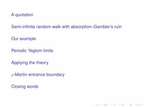
An evanescent process–Gambler’s ruin

I Suppose a gambler is pitted against an infinitely wealthycasino.

I The gambler enters the casino with x > 0 dollars.I With each play, the gambler either wins a dollar with

probability b where 0 < b < 1/2 . . .I . . . or loses a dollar with probability a where a+ b = 1.I The gambler continues to play for as long as possible.I In the long run the gambler is certainly broke.I What can be said about her fortune after playing many

times given that she still has at least one dollar?

A quasi-stationary distribution

I Seneta and Vere-Jones (1966) answered this question withthe following probability distribution π∗:

π∗(y) =1− ρa

y

(√b

a

)y−1for y = 1, 2, . . . (1)

I where a = 1− b and ρ = 2√ab.

Limiting conditional distributions

I Let Xn be her fortune after n plays.I Notice that her fortune alternates between being odd and

even.I For n large, Seneta and Vere-Jones proved that

Px{Xn = y | Xn ≥ 1} ≈

{π∗(y)π∗(2N) for y even, x+ n even,π∗(y)

π∗(2N−1) for y odd, x+ n odd.

I The subscript x means that X0 = x, N := {1, 2, . . .}.I The probability π assigns to the even and odd natural

numbers is denoted by π∗(2N) and π∗(2N−1), respectively.

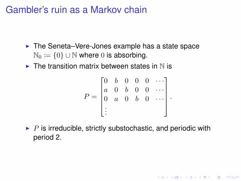
Gambler’s ruin as a Markov chain

I The Seneta–Vere-Jones example has a state spaceN0 := {0} ∪ N where 0 is absorbing.

I The transition matrix between states in N is

P =

0 b 0 0 0 · · ·a 0 b 0 0 · · ·0 a 0 b 0 · · ·...

.I P is irreducible, strictly substochastic, and periodic with

period 2.

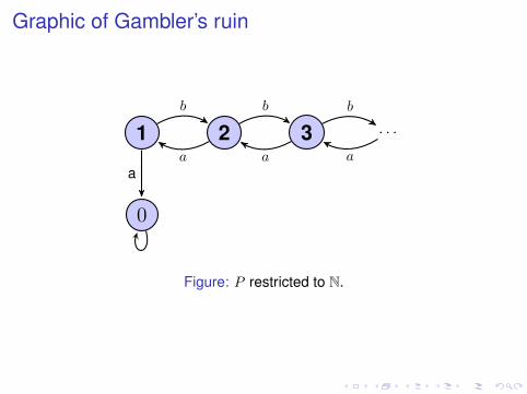
Graphic of Gambler’s ruin

1

0

2 3 . . .

b

a

b

a

b

a a

Figure: P restricted to N.

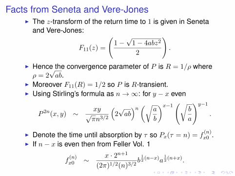
Facts from Seneta and Vere-JonesI The z-transform of the return time to 1 is given in Seneta

and Vere-Jones:

F11(z) =

(1−√1− 4abz2

2

).

I Hence the convergence parameter of P is R = 1/ρ whereρ = 2

√ab.

I Moreover F11(R) = 1/2 so P is R-transient.I Using Stirling’s formula as n→∞: for y − x even

P 2n(x, y) ∼ xy√πn3/2

(2√ab)n(√a

b

)x−1(√b

a

)y−1.

I Denote the time until absorption by τ so Px(τ = n) = f(n)x0 .

I If n− x is even then from Feller Vol. 1

f(n)x0 ∼ x · 2n+1

(2π)1/2(n)3/2b12(n−x)a

12(n+x).

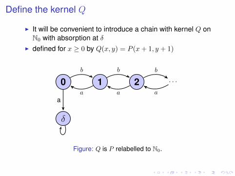
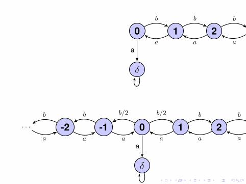
Define the kernel Q

I It will be convenient to introduce a chain with kernel Q onN0 with absorption at δ

I defined for x ≥ 0 by Q(x, y) = P (x+ 1, y + 1)

0

δ

1 2 . . .

b

a

b

a

b

a a

Figure: Q is P relabelled to N0.

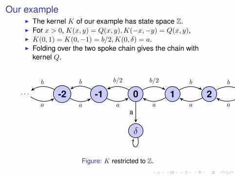
Our exampleI The kernel K of our example has state space Z.I For x > 0, K(x, y) = Q(x, y),K(−x,−y) = Q(x, y),I K(0, 1) = K(0,−1) = b/2,K(0, δ) = a.I Folding over the two spoke chain gives the chain with

kernel Q.

0

δ

1-1 2-2 . . .. . .

b/2b/2

a

b

a

b

a

b

a

b

a aa

Figure: K restricted to Z.

0

δ

1 2 . . .

b

a

b

a

b

a a

0

δ

1-1 2-2 . . .. . .

b/2b/2

a

b

a

b

a

b

a

b

a aa

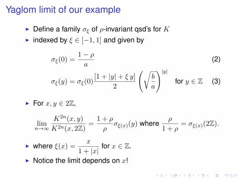
Yaglom limit of our example

I Define a family σξ of ρ-invariant qsd’s for KI indexed by ξ ∈ [−1, 1] and given by

σξ(0) =1− ρa

(2)

σξ(y) = σξ(0)[1 + |y|+ ξ y]

2

(√b

a

)|y|for y ∈ Z (3)

I For x, y ∈ 2Z,

limn→∞

K2n(x, y)

K2n(x, 2Z)=

1 + ρ

ρσξ(x)(y) where

ρ

1 + ρ= σξ(x)(2Z).

I where ξ(x) =x

1 + |x|for x ∈ Z.

I Notice the limit depends on x!

Definition of Periodic Yaglom limits

I For periodic chains, define k = k(x, y) ∈ {0, 1, 2, . . . d− 1}so that Knd+k(x, y) > 0 for n sufficiently large.

I We can partition S into d sets labeled S0, . . . , Sd−1 so thatthe starting state x ∈ S0 and that Knd+k(x, y) > 0 for nsufficiently large if y ∈ Sk.

I Theorem A of Vere-Jones implies that for any y ∈ Sk,[Knd+k(x, y)]1/(nd+k) → ρ.

I We say that we have a periodic Yaglom limit if for somek ∈ {0, . . . , d− 1}

Px{Xnd+k = y | Xnd+k ∈ S} =Knd+k(x, y)

Knd+k(x, S)→ πkx(y) (4)

where πkx is a probability measure on S with πkx(Sk) = 1.

Asymptotics of Periodic Yaglom limits

Proposition

I If πkx is the periodic Yaglom limit for somek ∈ {0, 1, . . . , d− 1}, then there are periodic Yaglom limitsfor all k ∈ {0, 1, . . . , d− 1}.

I Moreover, there is a ρ invariant qsd πx such thatπkx(y) = πx(y)/πx(Sk) for y ∈ Sk for eachk ∈ {0, 1, . . . , d− 1}.

I We concludeKnd+k(x, y)

Knd+k(x, S)→ πx(y)

πx(Sk)for all

k ∈ {0, 1, . . . , d− 1} where x ∈ S0 by definition and y ∈ Sk.

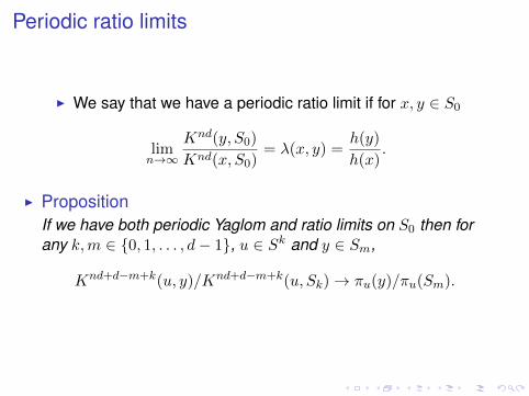
Periodic ratio limits

I We say that we have a periodic ratio limit if for x, y ∈ S0

limn→∞

Knd(y, S0)

Knd(x, S0)= λ(x, y) =

h(y)

h(x).

I PropositionIf we have both periodic Yaglom and ratio limits on S0 then forany k,m ∈ {0, 1, . . . , d− 1}, u ∈ Sk and y ∈ Sm,

Knd+d−m+k(u, y)/Knd+d−m+k(u, Sk)→ πu(y)/πu(Sm).

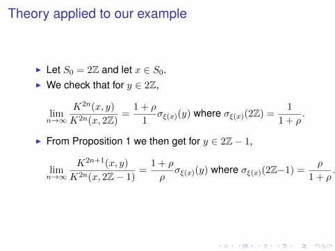
Theory applied to our example

I Let S0 = 2Z and let x ∈ S0.I We check that for y ∈ 2Z,

limn→∞

K2n(x, y)

K2n(x, 2Z)=

1 + ρ

1σξ(x)(y) where σξ(x)(2Z) =

1

1 + ρ.

I From Proposition 1 we then get for y ∈ 2Z− 1,

limn→∞

K2n+1(x, y)

K2n(x, 2Z− 1)=

1 + ρ

ρσξ(x)(y) where σξ(x)(2Z−1) =

ρ

1 + ρ.

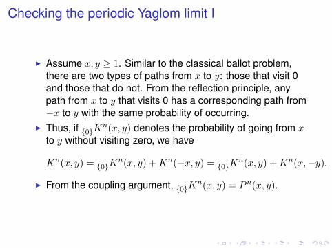
Checking the periodic Yaglom limit I

I Assume x, y ≥ 1. Similar to the classical ballot problem,there are two types of paths from x to y: those that visit 0and those that do not. From the reflection principle, anypath from x to y that visits 0 has a corresponding path from−x to y with the same probability of occurring.

I Thus, if {0}Kn(x, y) denotes the probability of going from x

to y without visiting zero, we have

Kn(x, y) = {0}Kn(x, y) +Kn(−x, y) = {0}K

n(x, y) +Kn(x,−y).

I From the coupling argument, {0}Kn(x, y) = Pn(x, y).

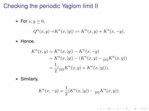
Checking the periodic Yaglom limit II

I For x, y ≥ 0,

Qn(x, y) =Kn(x, |y|) := Kn(x, y) +Kn(x,−y).

I Hence,

Kn(x, y) = Kn(x, |y|)−Kn(x,−y)= Kn(x, |y|)− (Kn(x, y)− {0}K

n(x, y))

=1

2({0}K

n(x, y) +Kn(x, |y|)).

I Similarly,

Kn(x,−y) = 1

2(Kn(x, |y|)− {0}K

n(x, y)).

Checking the periodic Yaglom limit III

I For x, y > 0 and both even, from (35) in Vere-Jones andSeneta

{0}K2n(x, y) = P 2n(x, y)

∼ xy√πn3/2

(2√ab)2n(√a

b

)x−1(√b

a

)y−1.

I Moreover,

K2n(x, |y|)) = Q2n(x, y) +Q2n(x,−y)= P 2n(x+ 1, y + 1) + P 2n(x+ 1,−(y + 1))

∼ (x+ 1)

(√a

b

)x(y + 1)

(√b

a

)y√1

π

(4ab)n

n3/2.

Checking the periodic Yaglom limit IV

I Let τδ be the time to absorption for the chain X. soPx(τδ = n) = Px+1(τ = n) and

Px(τδ > 2n) =

∞∑v=n+1

f2v−1x+1,0. (5)

Px(τ > 2n)

∼∞∑

v=n+1

(x+ 1) · 22v

(2π)1/2(2v − 1)3/2b12(2v−1−(x+1))a

12(2v−1+(x+1))

∼ (x+ 1)

(2π)1/2

(√a

b

)x(4ab)n

(2n)3/24a

1− 4ab.

Checking the periodic Yaglom limit V

I Hence, for x, y > 0,

K2n(x, y)

Px(τ > 2n)=

1

2

K2n(x, |y|)) + {0}K2n(x, y)

Px(τ > 2n)

∼

12(x+ 1)

(√ab

)x(y + 1)

(√ba

)y√1π(4ab)n

n3/2

(x+1)

(2π)1/2

(√ab

)x (4ab)n

(2n)3/24a

1−4ab

+

12

xy√πn3/2

(√ab)2n (

ab

)x/2 ( ba

)y/2(x+1)

(2π)1/2

(√ab

)x (4ab)n

(2n)3/24a

1−4ab

∼ 1− 4ab

a(1 + |y|+ ξy

2)

(√b

a

)y= (1 + ρ)σξ(x)(y).

Checking the periodic Yaglom limit VI

K2n(x,−y)Px(τ > 2n)

=1

2

(K2n(x, |y|)− {0}K2n(x, y)

Px(τ > 2n)

∼ (y + 1)

(√b

a

)y1− 4ab

2a− xy

x+ 1

(√b

a

)y1− 4ab

2a

=1− 4ab

a(1 + |y| − ξy

2)

(√b

a

)y= (1 + ρ)σξ(x)(−y).

Finally, for y = 0, K2n(x, 0) = P 2nx+1,1 so

K2n(x, 0)

Px(τ > 2n)=

P 2nx+1,1

Px(τ > 2n)=

(x+ 1)(√

ab

)x√ 1π(4ab)n

n3/2

(x+1)

(2π)1/2

(√ab

)x (4ab)n

(2n)3/24a

1−4ab

=1− 4ab

a= (1 + ρ)σξ(x)(0).

Checking the periodic Yaglom limit VII

I Therefore starting from x even we have a periodic Yaglomlimit with density (1 + 2

√ab)σξ(·) on S0 = 2Z with

ξ = x/(|x|+ 1) ∈ [0, 1].I Similarly, for x, y > 0 even, K2n(−x, y) = K2n(x,−y) andK2n(−x,−y) = K2n(x, y); hence, starting from −x evenwe get a Yaglom limit (1 + 2

√ab)σξ(·) on 2Z with

ξ = x/(|x|+ 1) so ξ ∈ [−1, 0].

Checking the periodic ratio limit

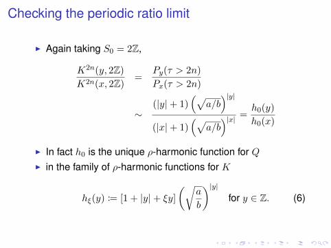
I Again taking S0 = 2Z,

K2n(y, 2Z)K2n(x, 2Z)

=Py(τ > 2n)

Px(τ > 2n)

∼(|y|+ 1)

(√a/b)|y|

(|x|+ 1)(√

a/b)|x| = h0(y)

h0(x)

I In fact h0 is the unique ρ-harmonic function for QI in the family of ρ-harmonic functions for K

hξ(y) := [1 + |y|+ ξy]

(√a

b

)|y|for y ∈ Z. (6)

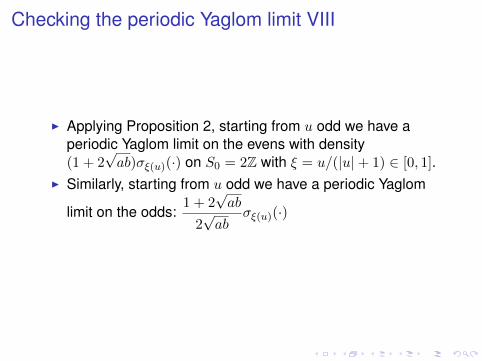
Checking the periodic Yaglom limit VIII

I Applying Proposition 2, starting from u odd we have aperiodic Yaglom limit on the evens with density(1 + 2

√ab)σξ(u)(·) on S0 = 2Z with ξ = u/(|u|+ 1) ∈ [0, 1].

I Similarly, starting from u odd we have a periodic Yaglom

limit on the odds:1 + 2

√ab

2√ab

σξ(u)(·)

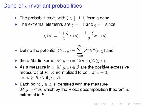
Cone of ρ-invariant probabilities

I The probabilities σξ with ξ ∈ [−1, 1] form a cone.I The extremal elements are ξ = −1 and ξ = 1 since

σξ(y) =1 + ξ

2σ1(y) +

1− ξ2

σ−1(y).

I Define the potential G(x, y) =∞∑n=0

RnKn(x, y) and

I the ρ-Martin kernel M(y, x) = G(y, x)/G(y, 0).I As a measure in x, M(y, x) ∈ B are the positive excessive

measures of R ·K normalized to be 1 at x = 0;i.e. µ ≥ RµK if µ ∈ B.

I Each point y ∈ Z is identified with the measureM(y, ·) ∈ B, which by the Riesz decomposition theorem isextremal in B.

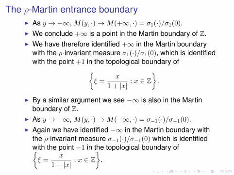
The ρ-Martin entrance boundaryI As y → +∞, M(y, ·)→M(+∞, ·) = σ1(·)/σ1(0).I We conclude +∞ is a point in the Martin boundary of Z.I We have therefore identified +∞ in the Martin boundary

with the ρ-invariant measure σ1(·)/σ1(0), which is identifiedwith the point +1 in the topological boundary of{

ξ =x

1 + |x|: x ∈ Z

}.

I By a similar argument we see −∞ is also in the Martinboundary of Z.

I As y → +∞, M(y, ·)→M(−∞, ·) = σ−1(·)/σ−1(0).I Again we have identified −∞ in the Martin boundary with

the ρ-invariant measure σ−1(·)/σ−1(0) which is identifiedwith the point −1 in the topological boundary of{ξ =

x

1 + |x|: x ∈ Z

}.

Harry Kesten’s exampleI Kesten (1995) constructed an amazing example of a

sub-Markov chain possessing most every niceproperty—including having a ρ-invariant qsd—that fails tohave a Yaglom limit.

I Kesten’s example has the same state space and the samestructure as ours.

I The only difference is that at any state x there is aprobability rx of holding in state x and probabilitiesa(1− rx) and b(1− rx) of moving one step closer or furtherfrom zero.

I If α = a(1− r0), then our chain is exactly Kesten’s chainwatched at the times his chain changes state.

I It is pretty clear Harry could have derived our example witha moment’s thought, but he focused on the non-existenceof Yaglom limits. His example is orders of magnitude moresophisticated and complicated than ours.