Distributional Generalization:A New Kind of Generalization

Preetum Nakkiran∗Harvard University

preetum@cs.harvard.edu

Yamini Bansal∗Harvard University

ybansal@g.harvard.edu

Abstract

We introduce a new notion of generalization— Distributional Generalization—which roughly states that outputs of a classifier at train and test time are close asdistributions, as opposed to close in just their average error. For example, if wemislabel 30% of dogs as cats in the train set of CIFAR-10, then a ResNet trained tointerpolation will in fact mislabel roughly 30% of dogs as cats on the test set as well,while leaving other classes unaffected. This behavior is not captured by classicalgeneralization, which would only consider the average error and not the distributionof errors over the input domain. Our formal conjectures, which are much moregeneral than this example, characterize the form of distributional generalizationthat can be expected in terms of problem parameters: model architecture, trainingprocedure, number of samples, and data distribution. We give empirical evidencefor these conjectures across a variety of domains in machine learning, includingneural networks, kernel machines, and decision trees. Our results thus advance ourempirical understanding of interpolating classifiers.

∗Co-first authors. Author contributions in Appendix A.

arX

iv:2

009.

0809

2v2

[cs

.LG

] 1

5 O

ct 2

020

1 Introduction

We begin with an experiment motivating the need for a notion of generalization beyond test error.

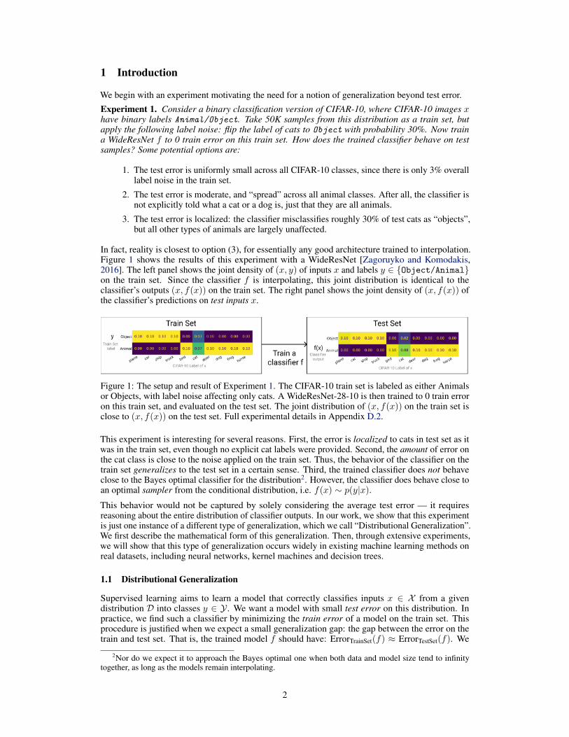
Experiment 1. Consider a binary classification version of CIFAR-10, where CIFAR-10 images xhave binary labels Animal/Object. Take 50K samples from this distribution as a train set, butapply the following label noise: flip the label of cats to Object with probability 30%. Now traina WideResNet f to 0 train error on this train set. How does the trained classifier behave on testsamples? Some potential options are:

1. The test error is uniformly small across all CIFAR-10 classes, since there is only 3% overalllabel noise in the train set.

2. The test error is moderate, and “spread” across all animal classes. After all, the classifier isnot explicitly told what a cat or a dog is, just that they are all animals.

3. The test error is localized: the classifier misclassifies roughly 30% of test cats as “objects”,but all other types of animals are largely unaffected.

In fact, reality is closest to option (3), for essentially any good architecture trained to interpolation.Figure 1 shows the results of this experiment with a WideResNet [Zagoruyko and Komodakis,2016]. The left panel shows the joint density of (x, y) of inputs x and labels y ∈ {Object/Animal}on the train set. Since the classifier f is interpolating, this joint distribution is identical to theclassifier’s outputs (x, f(x)) on the train set. The right panel shows the joint density of (x, f(x)) ofthe classifier’s predictions on test inputs x.

Figure 1: The setup and result of Experiment 1. The CIFAR-10 train set is labeled as either Animalsor Objects, with label noise affecting only cats. A WideResNet-28-10 is then trained to 0 train erroron this train set, and evaluated on the test set. The joint distribution of (x, f(x)) on the train set isclose to (x, f(x)) on the test set. Full experimental details in Appendix D.2.

This experiment is interesting for several reasons. First, the error is localized to cats in test set as itwas in the train set, even though no explicit cat labels were provided. Second, the amount of error onthe cat class is close to the noise applied on the train set. Thus, the behavior of the classifier on thetrain set generalizes to the test set in a certain sense. Third, the trained classifier does not behaveclose to the Bayes optimal classifier for the distribution2. However, the classifier does behave close toan optimal sampler from the conditional distribution, i.e. f(x) ∼ p(y|x).This behavior would not be captured by solely considering the average test error — it requiresreasoning about the entire distribution of classifier outputs. In our work, we show that this experimentis just one instance of a different type of generalization, which we call “Distributional Generalization”.We first describe the mathematical form of this generalization. Then, through extensive experiments,we will show that this type of generalization occurs widely in existing machine learning methods onreal datasets, including neural networks, kernel machines and decision trees.

1.1 Distributional Generalization

Supervised learning aims to learn a model that correctly classifies inputs x ∈ X from a givendistribution D into classes y ∈ Y . We want a model with small test error on this distribution. Inpractice, we find such a classifier by minimizing the train error of a model on the train set. Thisprocedure is justified when we expect a small generalization gap: the gap between the error on thetrain and test set. That is, the trained model f should have: ErrorTrainSet(f) ≈ ErrorTestSet(f). We

2Nor do we expect it to approach the Bayes optimal one when both data and model size tend to infinitytogether, as long as the models remain interpolating.

2

now re-write this classical notion of generalization in a form better suited for our extension.Classical Generalization: Let f be a trained classifier. Then f generalizes if:

Ex∼TrainSety←f(x)

[1{y 6= y(x)}] ≈ Ex∼TestSety←f(x)

[1{y 6= y(x)}] (1)

Above, y(x) is the true class of x and y is the predicted class. The LHS of Equation 1 is the trainerror of f , and the RHS is the test error. Crucially, both sides of Equation 1 are expectations of thesame function (Terr(x, y) := 1{y 6= y(x)}) under different distributions. The LHS of Equation 1is the expectation of Terr under the “Train Distribution” Dtr, which is the distribution over (x, y)given by sampling a train point x along with its classifier-label f(x). Similarly, the RHS is underthe “Test Distribution” Dte, which is this same construction over the test set. These two distributionsare the central objects in our study, and are defined formally in Section 3.2. We can now introduceDistributional Generalization, which is a property of trained classifiers. It is parameterized by a set ofbounded functions (“tests”): T ⊆ {T : X × Y → [0, 1]}.Distributional Generalization: Let f be a trained classifier. Then f satisfies Distributional Gener-alization with respect to tests T if:

∀T ∈ T : Ex∼TrainSety←f(x)

[T (x, y)] ≈ Ex∼TestSety←f(x)

[T (x, y)] (2)

We write this property as Dtr ≈T Dte. This states that the train and test distribution have similarexpectations for all functions in the family T . For the singleton set T = {Terr}, this is equivalent toclassical generalization, but it may hold for much larger sets T . For example in Experiment 1, thetrain and test distributions match with respect to the test function “Fraction of true cats labeled asobject.” In fact, we find that the family T is so large in practice that it is best to think of DistributionalGeneralization as stating that the distributions Dtr and Dte are close as distributions.

This property becomes especially interesting for interpolating classifiers, which fit their train setsexactly. Here, the Train Distribution (xi, f(xi)) is exactly equal3 to the original distribution (x, y) ∼D, since f(xi) = yi on the train set. In this case, distributional generalization claims that theoutput distribution (x, f(x)) of the model on test samples is close to the true distribution (x, y). Thefollowing conjecture specializes Distributional Generalization to interpolating classifiers, and will bethe main focus of our work.

Interpolating Indistinguishability Meta-Conjecture (informal): For interpolating classifiers f ,and a large family T of test functions, the distributions:

(x, f(x))x∈TestSet ≈T (x, f(x))x∈TrainSet ≡ (x, y)x,y∼D (3)

This is a “meta-conjecture”, which becomes a concrete conjecture once the family of tests T isspecified. One of the main contributions of our work is formally stating two concrete instances of thisconjecture— specifying exactly the family of tests T and their dependence on problem parameters(the distribution, model family, training procedure, etc). It captures behaviors far more general thanExperiment 1, and empirically applies across a variety of natural settings in machine learning.

1.2 Summary of Contributions

We extend the classical framework of generalization by introducing Distributional Generalization,in which the train and test behavior of models are close as distributions. Informally, for trainedclassifiers f , its outputs on the train set (x, f(x))x∈TrainSet are close in distribution to its outputs onthe test set (x, f(x))x∈TestSet, where the form of this closeness depends on specifics of the model,training procedure, and distribution. This notion is more fine-grained than classical generalization,since it considers the entire distribution of model outputs instead of just the test error.

We initiate the study of Distributional Generalization across various domains in machine learning.For interpolating classifiers, we state two formal conjectures which predict the form of distributionalcloseness that can be expected for a given model and task:

3The formal definition of Train Distribution, in Section 3.2, includes the randomness of sampling the trainset as well. We consider a fixed train set in the Introduction for sake of exposition.

3

1. Feature Calibration Conjecture (Section 4): Interpolating classifiers, when trained onsamples from a distribution, will match this distribution up to all “distinguishable features”(Definition 1).

2. Agreement Conjecture (Section 5): For two interpolating classifiers of the same type,trained independently on the same distribution, their agreement probability with each otheron test samples roughly matches their test accuracy.

We perform a number of experiments surrounding these conjectures, which reveal new behaviorsof standard interpolating classifiers (e.g. ResNets, MLPs, kernels, decision trees). We prove ourconjectures for 1-Nearest-Neighbors (Theorem 1), which suggests some form of “locality” as theunderlying mechanism. Finally, we discuss extending these results to non-interpolating methods inSection 7. Our experiments and conjectures shed new light on the structure of interpolating classifiers,which are extensively studied in recent years yet still poorly understood.

2 Related Work

Our work is inspired by the broader study of interpolating and overparameterized methods in machinelearning; a partial list of works in this theme includes Advani and Saxe [2017], Allen-Zhu et al. [2019],Arora et al. [2019], Bartlett et al. [2020], Belkin et al. [2018a,b, 2019], Breiman [1995], Chizat andBach [2020], Dziugaite and Roy [2017], Geiger et al. [2019], Gerace et al. [2020], Ghorbani et al.[2019], Goldt et al. [2019], Hastie et al. [2019], Ji and Telgarsky [2019], Liang and Rakhlin [2018],Mei and Montanari [2019], Muthukumar et al. [2020], Nakkiran et al. [2020], Neal et al. [2018],Neyshabur et al. [2018], Schapire et al. [1998], Soudry et al. [2018], Zhang et al. [2016].

Interpolating Methods. Many of the best-performing techniques on high-dimensional tasks areinterpolating methods, which fit their train samples to 0 train error. This includes neural networksand kernels on images [He et al., 2016, Shankar et al., 2020], and random forests on tabular data[Fernández-Delgado et al., 2014]. Interpolating methods have been extensively studied both recentlyand in the past, since we do not theoretically understand their practical success [Belkin et al., 2018a,b,2019, Breiman, 1995, Hastie et al., 2019, Liang and Rakhlin, 2018, Mei and Montanari, 2019,Nakkiran et al., 2020, Schapire, 1999, Schapire et al., 1998, Zhang et al., 2016]. In particular, muchof the classical work in statistical learning theory (uniform convergence, VC-dimension, Rademachercomplexity, regularization, stability) fails to explain the success of interpolating methods [Belkinet al., 2018a,b, Nagarajan and Kolter, 2019, Zhang et al., 2016]. The few techniques which do applyto interpolating methods (e.g. margin theory [Schapire et al., 1998]) remain vacuous on modernneural networks and kernels.

Learning Substructures. The observation that powerful networks can pick up on finer aspectsof the distribution than their training labels reveal also exists in various forms in the literature.For example, Gilboa and Gur-Ari [2019] found that standard CIFAR-10 networks tend to clusterleft-facing and right-facing horses separately in activation space, when visualized via activationatlases [Carter et al., 2019]. Such fine-structural aspects of distributions can also be seen at the levelof individual neurons (e.g. Bau et al. [2020], Cammarata et al. [2020], Olah et al. [2018], Radfordet al. [2017], Zhou et al. [2014]).

Decision Trees. In a similar vein to our work, Olson and Wyner [2018], Wyner et al. [2017]investigate decision trees, and show that random forests are equivalent to a Nadaraya–Watsonsmoother Nadaraya [1964], Watson [1964] with a certain smoothing kernel. Decision trees [Breimanet al., 1984] are often intuitively thought of as “adaptive nearest-neighbors,” since they are explicitlya spatial-partitioning method [Hastie et al., 2009]. Thus, it may not be surprising that decision treesbehave similarly to 1-Nearest-Neighbors. Olson and Wyner [2018], Wyner et al. [2017] took stepstowards characterizing and understanding this behavior – in particular, Olson and Wyner [2018]defines an equivalent smoothing kernel corresponding to a random forest, and empirically investigatesthe quality of the conditional density estimate. Our work presents a formal characterization of thequality of this conditional density estimate (Conjecture 1), which is a novel characterization even fordecision trees, as far as we know.

Kernel Smoothing. The term kernel regression is sometimes used in the literature to refer to kernelsmoothers, such as the Nadaraya–Watson kernel smoother [Nadaraya, 1964, Watson, 1964]. But in

4

this work we use the term “kernel regression” to refer only to regression in a Reproducing KernelHilbert Space, as described in the experimental details.

Label Noise. Our conjectures also describe the behavior of neural networks under label noise,which has been empirically and theoretically studied in the past, though not formally characterizedbefore [Belkin et al., 2018b, Chatterji and Long, 2020, Natarajan et al., 2013, Rolnick et al., 2017,Thulasidasan et al., 2019, Zhang et al., 2016, Ziyin et al., 2020]. Prior works have noticed thatvanilla interpolating networks are sensitive to label noise (e.g. Figure 1 in Zhang et al. [2016],and Belkin et al. [2018b]), and there are many works on making networks more robust to label noisevia modifications to the training procedure or objective [Natarajan et al., 2013, Rolnick et al., 2017,Thulasidasan et al., 2019, Ziyin et al., 2020]. In contrast, we claim this sensitivity to label noise isnot necessarily a problem to be fixed, but rather a consequence of a stronger property: distributionalgeneralization.

Conditional Density Estimation. Our density calibration property is similar to the guarantees of aconditional density estimator. More specifically, Conjecture 1 states that an interpolating classifiersamples from a distribution approximating the conditional density of p(y|x) in a certain sense.Conditional density estimation has been well-studied in classical nonparametric statistics (e.g. theNadaraya–Watson kernel smoother [Nadaraya, 1964, Watson, 1964]). However, these classicalmethods behave poorly in high-dimensions, both in theory and in practice. There are some attemptsto extend these classical methods to modern high-dimentional problems via augmenting estimatorswith neural networks (e.g. Rothfuss et al. [2019]). Random forests have also been known to exhibitproperties similar to conditional density estimators. This has been formalized in various ways, oftenonly with asymptotic guarantees [Athey et al., 2019, Meinshausen, 2006, Pospisil and Lee, 2018].

No prior work that we are aware of attempts to characterize the quality of the resulting densityestimate via testable assumptions, as we do with our formulation of Conjecture 1. Finally, ourmotivation is not to design good conditional density estimators, but rather to study properties ofinterpolating classifiers — which we find happen to share properties of density estimators.

Uncertainty and Calibration. The Agreement Property (Conjecture 2) bears some resemblance touncertainty estimation (e.g. Lakshminarayanan et al. [2017]), since it estimates the the test error of aclassifier using an ensemble of 2 models trained on disjoint train sets. However, there are importantcaveats: (1) Our Agreement Property only holds on-distribution, and degrades on off-distributioninputs. Thus, it is not as helpful to estimate out-of-distribution errors. (2) It only gives an estimate ofthe average test error, and does not imply pointwise calibration estimates for each sample.

Feature Calibration (Conjecture 1) is also related to the concepts of calibration and multicalibra-tion [Guo et al., 2017, Hébert-Johnson et al., 2018, Niculescu-Mizil and Caruana, 2005]. In ourframework, calibration is implied by Feature Calibration for a specific set of partitions L (determinedby level sets of the classifier’s confidence). However, we are not concerned with a specific set ofpartitions (or “subgroups” in the algorithmic fairness literature) but we generally aim to characterizefor which partitions Feature Calibration holds. Moreover, we consider only hard-classification deci-sions and not confidences, and we study only standard learning algorithms which are not given anydistinguished set of subgroups/partitions in advance. Our notion of distributional generalization isalso related to the notion of “distributional subgroup overfitting” introduced recently by Yaghini et al.[2019] to study algorithmic fairness. This can be seen as studying distributional generalization for aspecific family of tests (determined by distinguished subgroups in the population).

Locality and Manifold Learning. Our intuition for the behaviors in this work is that they arisedue to some form of “locality” of the trained classifiers, in an appropriate space. This intuition ispresent in various forms in the literature, for example: the so-called called “manifold hypothesis,”that natural data lie on a low-dimensional manifold (e.g. Narayanan and Mitter [2010], Sharma andKaplan [2020]), as well as works on local stiffness of the loss landscape [Fort et al., 2019b], andworks showing that overparameterized neural networks can learn hidden low-dimensional structurein high-dimensional settings [Bach, 2017, Chizat and Bach, 2020, Gerace et al., 2020]. It is open tomore formally understand connections between our work and the above.

5

3 Preliminaries

Notation. We consider joint distributions D on x ∈ X and discrete y ∈ Y = [k]. Let Dn denote niid samples from D and S = {(xi, yi)} denote a train set. Let F denote the training procedure ofa classifier family (including architecture and training algorithm), and let f ← TrainF (S) denotetraining a classifier f on train set S. We consider classifiers which output hard decisions f : X → Y .Let NNS(x) = xi denote the nearest neighbor to x in train-set S, with respect to a distance metricd. Our theorems will apply to any distance metric, and so we leave this unspecified. Let NN

(y)S (x)

denote the nearest neighbor estimator itself, that is, NN(y)S (x) := yi where xi = NNS(x).

Experimental Setup. Full experimental details are provided in Appendix C. Briefly, we train allclassifiers to interpolation unless otherwise specified— that is, to 0 train error. We use standard-practice training techniques for all methods with minor hyperparameter modifications for trainingto interpolation. In all experiments, we consider only the hard-classification decisions, and note.g. the softmax probabilities. Neural networks (MLPs and ResNets [He et al., 2016]) are trainedwith Stochastic Gradient Descent. Interpolating decision trees are trained using the growth rulefrom Random Forests [Breiman, 2001], growing until all leafs have a single sample. For kernelclassification, we consider both kernel regression on one-hot labels and kernel SVM, with small or0 values of regularization (which is often optimal, as in Shankar et al. [2020]). Section 7 considersnon-interpolating versions of the above methods (via early-stopping or regularization).

3.1 Distributional Closeness

For two distributions P,Q over X × Y , let P ≈ε Q denote ε-closeness in total variation distance;that is, TV (P,Q) = 1

2 ||P − Q||1 ≤ ε. Recall that TV-distance has an equivalent variationalcharacterization: For distributions P,Q over X × Y , we have

TV (P,Q) = supT :X×Y→[0,1]

∣∣∣∣ E(x,y)∼P

[T (x, y)]− E(x,y)∼Q

[T (x, y)]

∣∣∣∣A “test” (or “distinguisher”) here is a function T : X × Y → [0, 1] which accepts a sample fromeither distribution, and is intended to classify the sample as either from distribution P or Q. TVdistance is then the advantage of the best distinguisher among all bounded tests. More generally, forany family T ⊆ {T : X ×Y → [0, 1]} of tests, we say distributions P andQ are “ε-indistinguishableup to T -tests” if they are close with respect to all tests in class T . That is,

P ≈Tε Q ⇐⇒ supT∈T

∣∣∣∣ E(x,y)∼P

[T (x, y)]− E(x,y)∼Q

[T (x, y)]

∣∣∣∣ ≤ ε (4)

This notion of closeness is also known as an Integral Probability Metric [Müller, 1997]. Throughoutthis work, we will define specific families of distinguishers T to characterize the sense in whichthe output distribution (x, f(x)) of classifiers is close to their input distribution (x, y) ∼ D. Whenwe write P ≈ Q, we are making an informal claim in which we mean P ≈ε Q for some small butunspecified ε.

3.2 Framework for Indistinguishability

Here we setup the formal objects studied in the remainder of the paper. This formal description ofTrain and Test distributions differs slightly from the informal description in the Introduction, becausewe want to study the generalization properties of an entire end-to-end training procedure (TrainF ),and not just properties of a fixed classifier (f ). We thus consider the following three distributionsover X × Y .

Source D: (x, y)where x, y ∼ D

Train Dtr: (xtr, f(xtr))S ∼ Dn, f ← TrainF (S),xtr, ytr ∼ S

Test Dte (x, f(x))S ∼ Dn, f ← TrainF (S),x, y ∼ D

The Source Distribution D is simply the original distribution. To sample from the Train Distribu-tion Dtr, we first sample a train set S ∼ Dn, train a classifier f on it, then output (xtr, f(xtr)) for arandom train point xtr. That is, Dtr is the distribution of input and outputs of a trained classifier f

6

on its train set. To sample from the Test Distribution Dte, do we this same procedure, but output(x, f(x)) for a random test point x. That is, theDte is the distribution of input and outputs of a trainedclassifier f at test time. The only difference between the Train Distribution and Test Distribution isthat the point x is sampled from the train set or the test set, respectively.4

For interpolating classifiers, f(xtr) = ytr on the train set, and so the Source and Train distributionsare equivalent:

For interpolating classifiers f : D ≡ Dtr (5)

Our general thesis is that the Train and Test Distributions are indistinguishable under a variety of testfamilies T . Formally, we argue that for certain families of tests T and interpolating classifiers F ,

Indistinguishability Conjecture: D ≡ Dtr ≈Tε Dte (6)

Sections 4 and 5 give specific families of tests T for which these distributions are indistinguish-able. The quality of this distributional closeness will depend on details of the classifier family anddistribution, in ways which we will specify.

4 Feature Calibration

The distributional closeness of Experiment 1 is subtle, and depends on the classifier architecture,distribution, and training method. For example, Experiment 1 does not hold if we use a fully-connected network (MLP) instead of a ResNet, or if we early-stop the ResNet instead of trainingto interpolation (see Appendix D.2). Both these scenarios fail in different ways: An MLP cannotproperly distinguish cats from dogs even when trained on real CIFAR-10 labels, and so (informally)it has no hope of behaving differently on cats in the setting of Experiment 1. On the other hand, anearly-stopped ResNet for Experiment 1 does not label 30% of cats as objects on the train set, since itdoes not interpolate, and thus has no hope of reproducing this behavior on the test set.

We now characterize these behaviors, and their dependency on problem parameters, via a formalconjecture. This conjecture characterizes a family of tests T for which the output distribution of aclassifier (x, f(x)) ∼ Dte is “close” to the source distribution (x, y) ∼ D. At a high level, we arguethat the distributions Dte and D are statistically close if we first “coarsen” the domain of x by somelabelling L : X → [M ]. That is, for certain partitions L, the following distributions are statisticallyclose:

(L(x), f(x)) ≈ε (L(x), y)

We first explain this conjecture (“Feature Calibration”) via a toy example, and then we state theconjecture formally in Section 4.2.

4.1 Toy Example

Consider a distribution on points x ∈ R2 and binary labels y, as visualized in Figure 2A. Thisdistribution consists of four clusters {Truck, Ship, Cat, Dog} which are labeled either Objector Animal, depicted in red and blue respectively. One of these clusters — the Cat cluster — ismislabeled as class Object with probability 30%. Now suppose we have an interpolating classifier ffor this distribution, obtained in some way, and we wish to quantify the closeness between distributions(x, y) ≈ (x, f(x)) on the test set. Figure 2A shows test points x along with their test labels y – theseare samples from the source distribution D. Figure 2B shows these same test points, but labeledaccording to f(x) – these are samples from the test distribution Dte. The shaded red/blue regions inFigure 2B shows the decision boundary of the classifier f .

These two distributions do not match exactly – there are some test points where the true label yand classifier output f(x) disagree. However, if we “coarsen” the domain into the four clusters{Truck, Ship, Cat, Dog}, then the marginal distribution of labels within each cluster matches

4Technically, these definitions require training a fresh classifier for each sample, using independent train sets.We use this definition because we believe it is natural, although for practical reasons most of our experimentstrain a single classifier f and evaluate it on the entire train/test set.

7

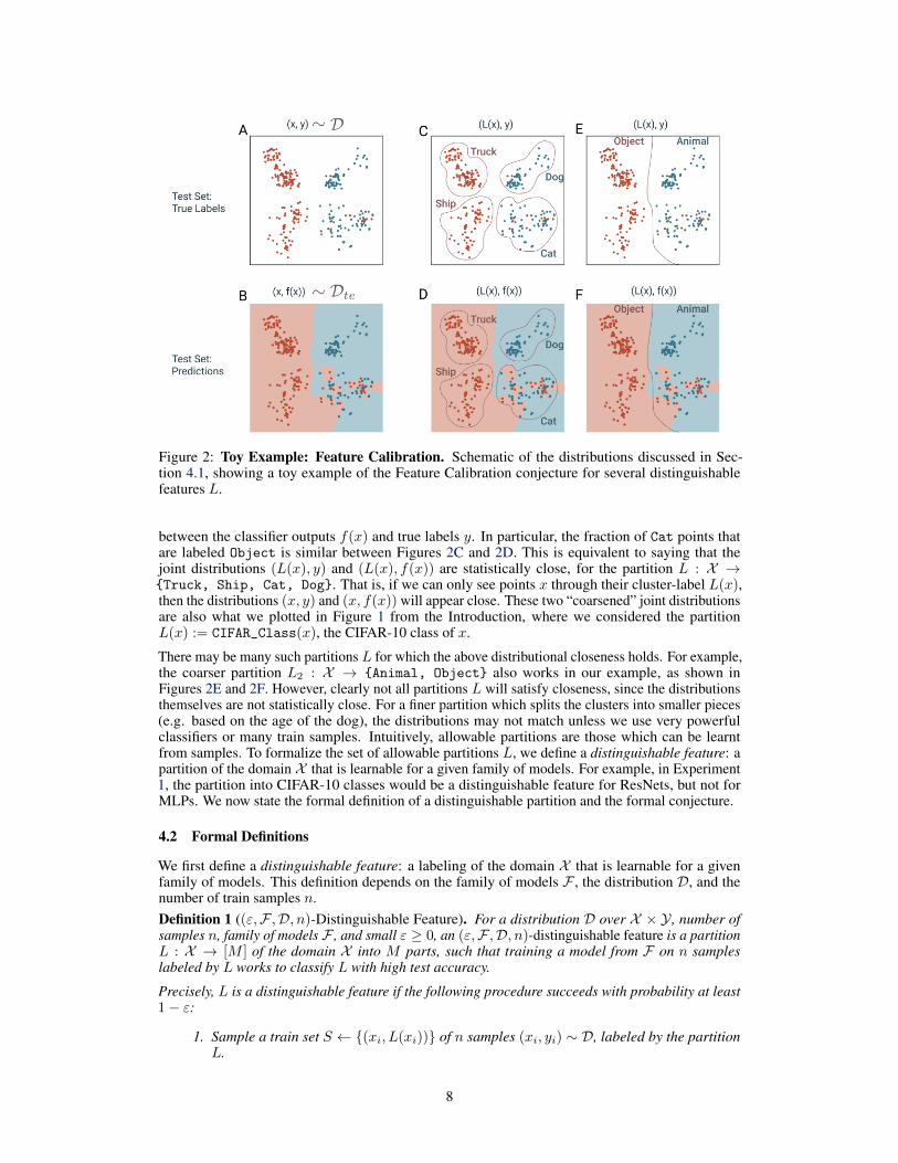
Figure 2: Toy Example: Feature Calibration. Schematic of the distributions discussed in Sec-tion 4.1, showing a toy example of the Feature Calibration conjecture for several distinguishablefeatures L.

between the classifier outputs f(x) and true labels y. In particular, the fraction of Cat points thatare labeled Object is similar between Figures 2C and 2D. This is equivalent to saying that thejoint distributions (L(x), y) and (L(x), f(x)) are statistically close, for the partition L : X →{Truck, Ship, Cat, Dog}. That is, if we can only see points x through their cluster-label L(x),then the distributions (x, y) and (x, f(x)) will appear close. These two “coarsened” joint distributionsare also what we plotted in Figure 1 from the Introduction, where we considered the partitionL(x) := CIFAR_Class(x), the CIFAR-10 class of x.

There may be many such partitions L for which the above distributional closeness holds. For example,the coarser partition L2 : X → {Animal, Object} also works in our example, as shown inFigures 2E and 2F. However, clearly not all partitions L will satisfy closeness, since the distributionsthemselves are not statistically close. For a finer partition which splits the clusters into smaller pieces(e.g. based on the age of the dog), the distributions may not match unless we use very powerfulclassifiers or many train samples. Intuitively, allowable partitions are those which can be learntfrom samples. To formalize the set of allowable partitions L, we define a distinguishable feature: apartition of the domain X that is learnable for a given family of models. For example, in Experiment1, the partition into CIFAR-10 classes would be a distinguishable feature for ResNets, but not forMLPs. We now state the formal definition of a distinguishable partition and the formal conjecture.

4.2 Formal Definitions

We first define a distinguishable feature: a labeling of the domain X that is learnable for a givenfamily of models. This definition depends on the family of models F , the distribution D, and thenumber of train samples n.Definition 1 ((ε,F ,D, n)-Distinguishable Feature). For a distribution D over X × Y , number ofsamples n, family of models F , and small ε ≥ 0, an (ε,F ,D, n)-distinguishable feature is a partitionL : X → [M ] of the domain X into M parts, such that training a model from F on n sampleslabeled by L works to classify L with high test accuracy.

Precisely, L is a distinguishable feature if the following procedure succeeds with probability at least1− ε:

1. Sample a train set S ← {(xi, L(xi))} of n samples (xi, yi) ∼ D, labeled by the partitionL.

8

2. Train a classifier f ← TrainF (S).

3. Sample a test point x ∼ D, and check that f correctly classifies its partition: Output successiff f(x) = L(x).

That is, L is a (ε,F ,D, n)-distinguishable feature if:

PrS={(xi,L(xi)}x1,...,xn∼D

f←TrainF (S)x∼D

[f(x) = L(x)] ≥ 1− ε

To recap, this definition is meant to capture a labeling of the domain X that is learnable for a givenfamily of models and training procedure. Note that this definition only depends on the marginaldistribution of D on x, and does not depend on the label distribution pD(y|x). The definition ofdistinguishable feature must depend on the classifier family F and number of samples n, since amore powerful classifier can distinguish more features. Note that there could be many distinguishablefeatures for a given setting (ε,F ,D, n) — including features not implied by the class label, such asthe presence of grass in a CIFAR-10 image.

Our main conjecture in this section is that the test distribution (x, f(x)) ∼ Dte is statistically close tothe source distribution (x, y) ∼ D when the domain is “coarsened” by a distinguishable feature. Thatis, the distributions (L(x), f(x)) and (L(x), y) are statistically close for all distinguishable featuresL. Formally:Conjecture 1 (Feature Calibration). For all natural distributions D, number of samples n, familyof interpolating models F , and ε ≥ 0, the following distributions are statistically close for all(ε,F ,D, n)-distinguishable features L:

(L(x), f(x))f←TrainF (Dn)

x,y∼D

≈ε (L(x), y)x,y∼D

(7)

Notably, this holds for all distinguishable features L, and it holds “automatically” – we simply train aclassifier, without specifying any particular partition. The statistical closeness predicted is within ε,which is determined by the ε-distinguishability of L (we usually think of ε as small). As a trivialinstance of the conjecture, suppose we have a distribution with deterministic labels, and consider theε-distinguishable feature L(x) := y(x), i.e. the label itself. The ε here is then simply the test error off , and Conjecture 1 is true by definition. The formal statements of Definition 1 and Conjecture 1may seem somewhat arbitrary, involving many quantifiers over (ε,F ,D, n). However, we believethese statements are natural. To support this, in Section 4.5 we prove that Conjecture 1 is formallytrue as stated for 1-Nearest-Neighbor classifiers.

Connection to Indistinguishability. Conjecture 1 can be equivalently phrased as an instantiationof our general Indistinguishably Conjecture: the source distribution D and test distribution Dte are“indistinguishable up to L-tests”. That is, Conjecture 1 is equivalent to the statement

Dte ≈Lε D (8)

where L is the family of all tests which depend on x only via a distinguishable feature L. That is,L := {(x, y) 7→ T (L(x), y) : (ε,F ,D, n)-distinguishable feature L and T : [M ]× Y → [0, 1]}. Inother words, Dte is indistinguishable from D to any distinguisher that only sees the input x via adistinguishable feature L(x).

4.3 Experiments

We now empirically validate our conjecture in a variety of settings in machine learning, includingneural networks, kernel machines, and decision trees. To do so, we begin by considering thesimplest possible distinguishable feature, and progressively consider more complex ones. Each ofthe experimental settings below highlights a different aspect of interpolating classifiers, which maybe of independent theoretical or practical interest. We summarize the experiments here; detaileddescriptions are provided in Appendix D.

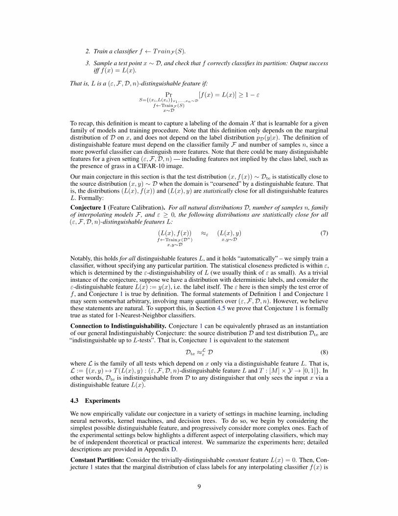
Constant Partition: Consider the trivially-distinguishable constant feature L(x) = 0. Then, Con-jecture 1 states that the marginal distribution of class labels for any interpolating classifier f(x) is

9

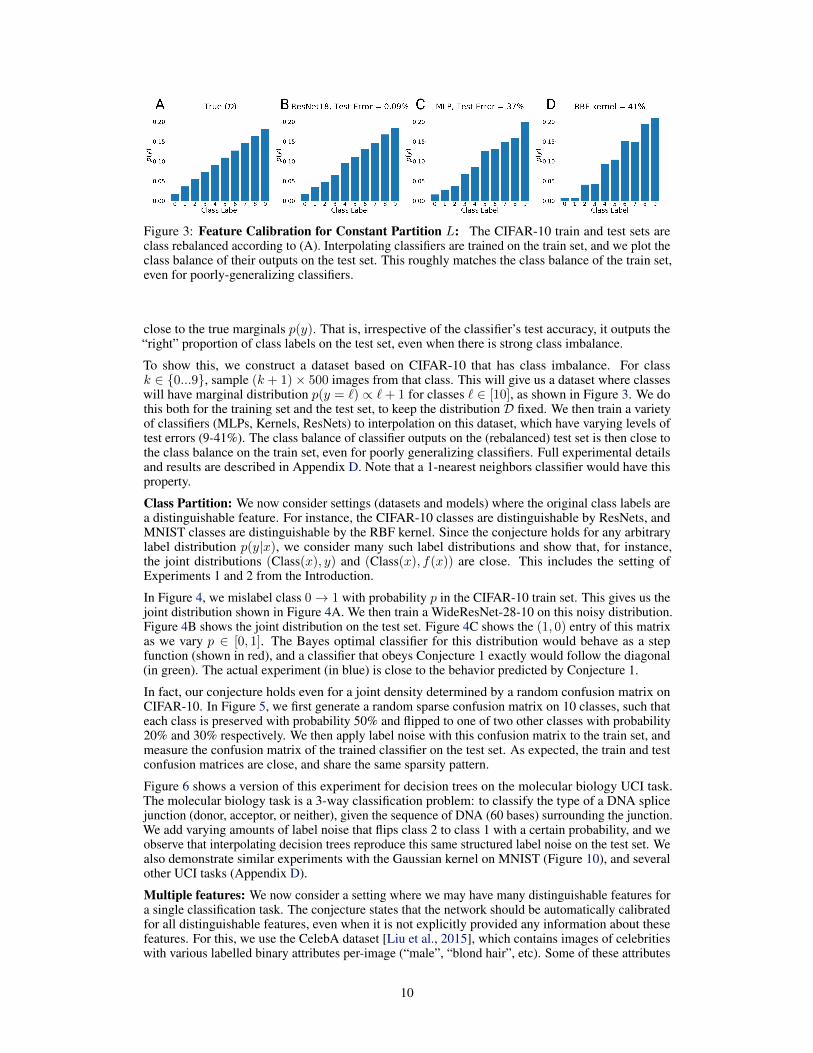
Figure 3: Feature Calibration for Constant Partition L: The CIFAR-10 train and test sets areclass rebalanced according to (A). Interpolating classifiers are trained on the train set, and we plot theclass balance of their outputs on the test set. This roughly matches the class balance of the train set,even for poorly-generalizing classifiers.

close to the true marginals p(y). That is, irrespective of the classifier’s test accuracy, it outputs the“right” proportion of class labels on the test set, even when there is strong class imbalance.

To show this, we construct a dataset based on CIFAR-10 that has class imbalance. For classk ∈ {0...9}, sample (k + 1)× 500 images from that class. This will give us a dataset where classeswill have marginal distribution p(y = `) ∝ `+ 1 for classes ` ∈ [10], as shown in Figure 3. We dothis both for the training set and the test set, to keep the distribution D fixed. We then train a varietyof classifiers (MLPs, Kernels, ResNets) to interpolation on this dataset, which have varying levels oftest errors (9-41%). The class balance of classifier outputs on the (rebalanced) test set is then close tothe class balance on the train set, even for poorly generalizing classifiers. Full experimental detailsand results are described in Appendix D. Note that a 1-nearest neighbors classifier would have thisproperty.

Class Partition: We now consider settings (datasets and models) where the original class labels area distinguishable feature. For instance, the CIFAR-10 classes are distinguishable by ResNets, andMNIST classes are distinguishable by the RBF kernel. Since the conjecture holds for any arbitrarylabel distribution p(y|x), we consider many such label distributions and show that, for instance,the joint distributions (Class(x), y) and (Class(x), f(x)) are close. This includes the setting ofExperiments 1 and 2 from the Introduction.

In Figure 4, we mislabel class 0→ 1 with probability p in the CIFAR-10 train set. This gives us thejoint distribution shown in Figure 4A. We then train a WideResNet-28-10 on this noisy distribution.Figure 4B shows the joint distribution on the test set. Figure 4C shows the (1, 0) entry of this matrixas we vary p ∈ [0, 1]. The Bayes optimal classifier for this distribution would behave as a stepfunction (shown in red), and a classifier that obeys Conjecture 1 exactly would follow the diagonal(in green). The actual experiment (in blue) is close to the behavior predicted by Conjecture 1.

In fact, our conjecture holds even for a joint density determined by a random confusion matrix onCIFAR-10. In Figure 5, we first generate a random sparse confusion matrix on 10 classes, such thateach class is preserved with probability 50% and flipped to one of two other classes with probability20% and 30% respectively. We then apply label noise with this confusion matrix to the train set, andmeasure the confusion matrix of the trained classifier on the test set. As expected, the train and testconfusion matrices are close, and share the same sparsity pattern.

Figure 6 shows a version of this experiment for decision trees on the molecular biology UCI task.The molecular biology task is a 3-way classification problem: to classify the type of a DNA splicejunction (donor, acceptor, or neither), given the sequence of DNA (60 bases) surrounding the junction.We add varying amounts of label noise that flips class 2 to class 1 with a certain probability, and weobserve that interpolating decision trees reproduce this same structured label noise on the test set. Wealso demonstrate similar experiments with the Gaussian kernel on MNIST (Figure 10), and severalother UCI tasks (Appendix D).

Multiple features: We now consider a setting where we may have many distinguishable features fora single classification task. The conjecture states that the network should be automatically calibratedfor all distinguishable features, even when it is not explicitly provided any information about thesefeatures. For this, we use the CelebA dataset [Liu et al., 2015], which contains images of celebritieswith various labelled binary attributes per-image (“male”, “blond hair”, etc). Some of these attributes

10

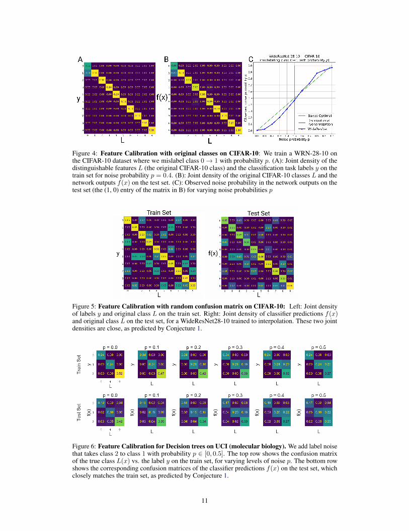
Figure 4: Feature Calibration with original classes on CIFAR-10: We train a WRN-28-10 onthe CIFAR-10 dataset where we mislabel class 0→ 1 with probability p. (A): Joint density of thedistinguishable features L (the original CIFAR-10 class) and the classification task labels y on thetrain set for noise probability p = 0.4. (B): Joint density of the original CIFAR-10 classes L and thenetwork outputs f(x) on the test set. (C): Observed noise probability in the network outputs on thetest set (the (1, 0) entry of the matrix in B) for varying noise probabilities p

Figure 5: Feature Calibration with random confusion matrix on CIFAR-10: Left: Joint densityof labels y and original class L on the train set. Right: Joint density of classifier predictions f(x)and original class L on the test set, for a WideResNet28-10 trained to interpolation. These two jointdensities are close, as predicted by Conjecture 1.

Figure 6: Feature Calibration for Decision trees on UCI (molecular biology). We add label noisethat takes class 2 to class 1 with probability p ∈ [0, 0.5]. The top row shows the confusion matrixof the true class L(x) vs. the label y on the train set, for varying levels of noise p. The bottom rowshows the corresponding confusion matrices of the classifier predictions f(x) on the test set, whichclosely matches the train set, as predicted by Conjecture 1.

11

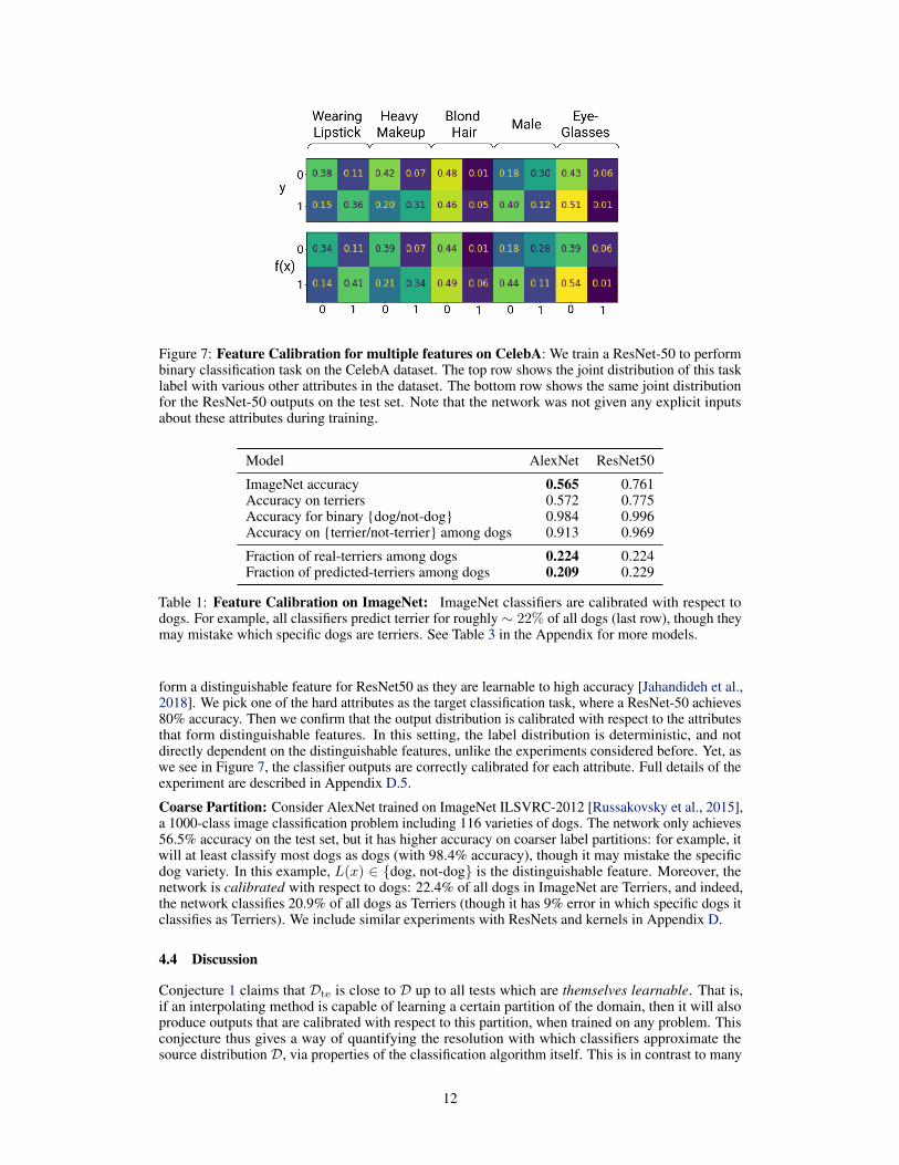
Figure 7: Feature Calibration for multiple features on CelebA: We train a ResNet-50 to performbinary classification task on the CelebA dataset. The top row shows the joint distribution of this tasklabel with various other attributes in the dataset. The bottom row shows the same joint distributionfor the ResNet-50 outputs on the test set. Note that the network was not given any explicit inputsabout these attributes during training.

Model AlexNet ResNet50

ImageNet accuracy 0.565 0.761Accuracy on terriers 0.572 0.775Accuracy for binary {dog/not-dog} 0.984 0.996Accuracy on {terrier/not-terrier} among dogs 0.913 0.969

Fraction of real-terriers among dogs 0.224 0.224Fraction of predicted-terriers among dogs 0.209 0.229

Table 1: Feature Calibration on ImageNet: ImageNet classifiers are calibrated with respect todogs. For example, all classifiers predict terrier for roughly ∼ 22% of all dogs (last row), though theymay mistake which specific dogs are terriers. See Table 3 in the Appendix for more models.

form a distinguishable feature for ResNet50 as they are learnable to high accuracy [Jahandideh et al.,2018]. We pick one of the hard attributes as the target classification task, where a ResNet-50 achieves80% accuracy. Then we confirm that the output distribution is calibrated with respect to the attributesthat form distinguishable features. In this setting, the label distribution is deterministic, and notdirectly dependent on the distinguishable features, unlike the experiments considered before. Yet, aswe see in Figure 7, the classifier outputs are correctly calibrated for each attribute. Full details of theexperiment are described in Appendix D.5.

Coarse Partition: Consider AlexNet trained on ImageNet ILSVRC-2012 [Russakovsky et al., 2015],a 1000-class image classification problem including 116 varieties of dogs. The network only achieves56.5% accuracy on the test set, but it has higher accuracy on coarser label partitions: for example, itwill at least classify most dogs as dogs (with 98.4% accuracy), though it may mistake the specificdog variety. In this example, L(x) ∈ {dog, not-dog} is the distinguishable feature. Moreover, thenetwork is calibrated with respect to dogs: 22.4% of all dogs in ImageNet are Terriers, and indeed,the network classifies 20.9% of all dogs as Terriers (though it has 9% error in which specific dogs itclassifies as Terriers). We include similar experiments with ResNets and kernels in Appendix D.

4.4 Discussion

Conjecture 1 claims that Dte is close to D up to all tests which are themselves learnable. That is,if an interpolating method is capable of learning a certain partition of the domain, then it will alsoproduce outputs that are calibrated with respect to this partition, when trained on any problem. Thisconjecture thus gives a way of quantifying the resolution with which classifiers approximate thesource distribution D, via properties of the classification algorithm itself. This is in contrast to many

12

classical ways of quantifying the approximation of density estimators, which rely on analytic (ratherthan operational) distributional assumptions [Tsybakov, 2008, Wasserman, 2006].

Proper Scoring Rules. If the loss function used in training is a strictly-proper scoring rule suchas cross-entropy [Gneiting and Raftery, 2007], then we may expect that in the limit of a large-capacity network and infinite data, training on samples {(xi, yi)} will yield a good density estimateof p(y|x) at the softmax layer. However, this is not what is happening in our experiments: First, ourexperiments consider the hard-decisions, not the softmax outputs. Second, we observe Conjecture 1even in settings without proper scoring rules (e.g. kernel SVM and decision trees).

4.5 1-Nearest-Neighbors Connection

Here we show that the 1-nearest neighbor classifier provably satisfies Conjecture 1, under mildassumptions. This is trivially true when the number of train points n→∞, such that the train pointspack the domain. However, we do not require any such assumptions: the theorem below appliesgenerically to a wide class of distributions, with no assumptions on the ambient dimension of inputs,the underlying metric, or smoothness of the source distribution. All the distributional requirements arecaptured by the preconditions of Conjecture 1, which require that the feature L is ε-distinguishableto 1-Nearest-Neighbors. The only further assumption is a weak regularity condition: sampling thenearest neighbor train point to a random test point should yield (close to) a uniformly random testpoint. In the following, NNS(x) refers to the nearest neighbor of point x among points in set S.Theorem 1. Let D be a distribution over X × Y , and let n ∈ N be the number of train samples.Assume the following regularity condition holds: Sampling the nearest neighbor train point to arandom test point yields (close to) a uniformly random test point. That is, suppose that for somesmall δ ≥ 0,

{NNS(x)}S∼Dn

x∼D≈δ {x}x∼D (9)

Then, Conjecture 1 holds. For all (ε,NN,D, n)-distinguishable partitions L, the following distribu-tions are statistically close:

{(y, L(x))}x,y∼D ≈ε+δ {(NN(y)S (x), L(x)}S∼Dn

x,y∼D(10)

The proof of Theorem 1 is straightforward, and provided in Appendix G. We view this theorem bothas support for our formalism of Conjecture 1, and as evidence that the classifiers we consider in thiswork have local properties similar to 1-Nearest-Neighbors.

Note that Theorem 1 does not hold for the k-nearest neighbor classifier (k-NN), which takes theplurality vote of K neighboring train points. However, it is somewhat more general than 1-NN: forexample, it holds for a randomized version of k-NN which, instead of taking the plurality, randomlypicks one of the K neighboring train points (potentially weighted) for the test classification.

4.6 Pointwise Density Estimation

In fact, we could hope for an even stronger property than Conjecture 1. Consider the familiar example:we mislabel 20% of dogs as cats in the CIFAR-10 training data, and train an interpolating ResNeton this train set. Conjecture 1 predicts that, on average over all test dogs, roughly 20% of them areclassified as cats. In fact, we may expect this to hold pointwise for each dog: For a single test dog x,if we train a new classifier f (on fresh iid samples from the noisy distribution), then f(x) will be catroughly 20% of the time. That is, for each test point x, taking an ensemble over independent trainsets yields an estimate of the conditional density p(y|x). Informally:

With high probability over test x ∼ D : Prf←TrainF (Dn)

[f(x) = `] ≈ p(y = `|x) (11)

where the probability on the LHS is over the random sampling of train set, and any randomness inthe training procedure. This behavior would be stronger than, and not implied by, Conjecture 1. Wegive preliminary experiments supporting such a pointwise property in Appendix D.7.

5 Agreement Property

We now present an “agreement property” of various classifiers. This property is independent of theprevious section, though both are instantiations of our general indistinguishability conjecture. We

13

claim that, informally, the test accuracy of a classifier is close to the probability that it agrees with anidentically-trained classifier on a disjoint train set.Conjecture 2 (Agreement Property). For certain classifier families F and distributions D, the testaccuracy of a classifier is close to its agreement probability with an independently-trained classifier.That is, let S1, S2 be independent train sets sampled from Dn, and let f1, f2 be classifiers trained onS1, S2 respectively. Then

PrS1∼Dn

f1←TrainF (S1)(x,y)∼D

[f1(x) = y] ≈ PrS1,S2∼Dn

fi←TrainF (Si)(x,y)∼D

[f1(x) = f2(x)] (12)

Moreover, this holds with high probability over training f1, f2: Pr(x,y)∼D[f1(x) = y] ≈Pr(x,y)∼D[f1(x) = f2(x)].

(a) ResNet18 on CIFAR-10. (b) ResNet18 on CIFAR-100. (c) Myrtle Kernel on CIFAR-10.

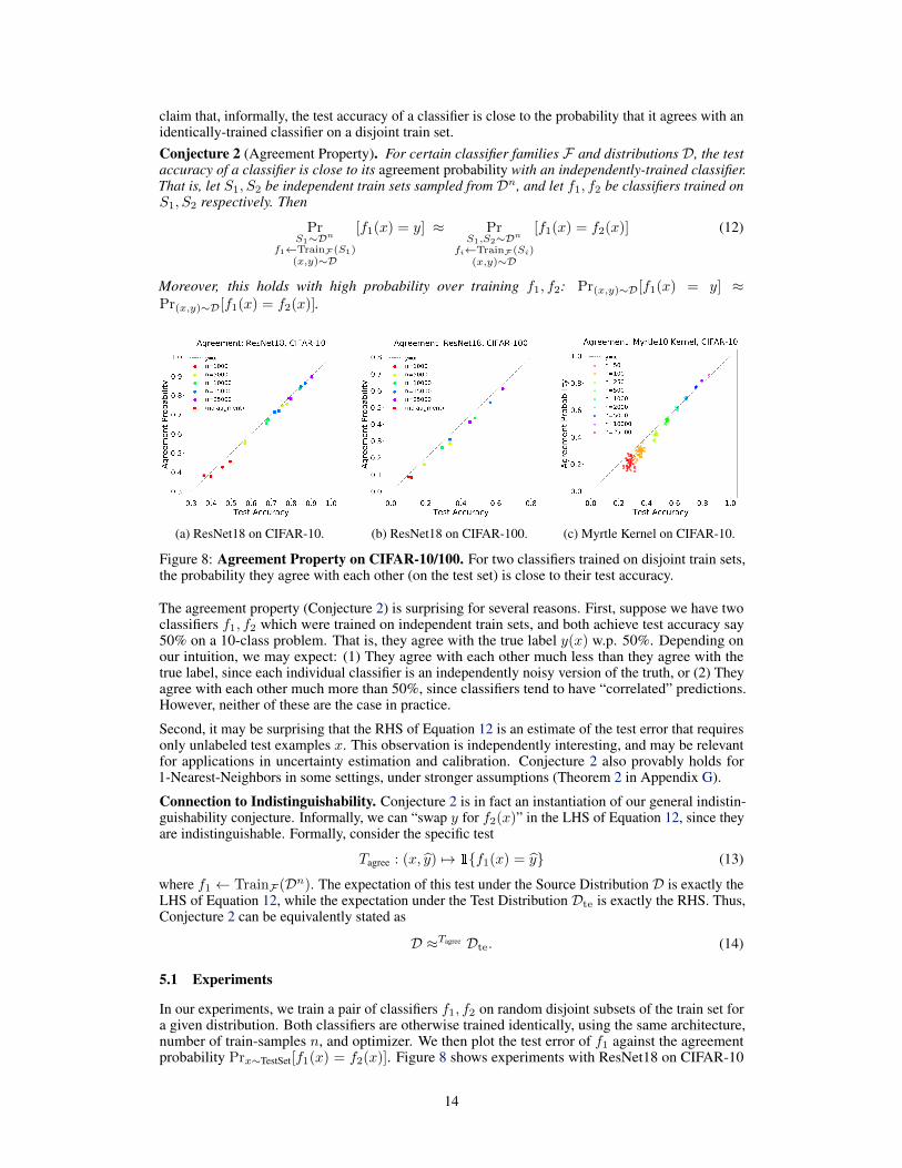
Figure 8: Agreement Property on CIFAR-10/100. For two classifiers trained on disjoint train sets,the probability they agree with each other (on the test set) is close to their test accuracy.

The agreement property (Conjecture 2) is surprising for several reasons. First, suppose we have twoclassifiers f1, f2 which were trained on independent train sets, and both achieve test accuracy say50% on a 10-class problem. That is, they agree with the true label y(x) w.p. 50%. Depending onour intuition, we may expect: (1) They agree with each other much less than they agree with thetrue label, since each individual classifier is an independently noisy version of the truth, or (2) Theyagree with each other much more than 50%, since classifiers tend to have “correlated” predictions.However, neither of these are the case in practice.

Second, it may be surprising that the RHS of Equation 12 is an estimate of the test error that requiresonly unlabeled test examples x. This observation is independently interesting, and may be relevantfor applications in uncertainty estimation and calibration. Conjecture 2 also provably holds for1-Nearest-Neighbors in some settings, under stronger assumptions (Theorem 2 in Appendix G).

Connection to Indistinguishability. Conjecture 2 is in fact an instantiation of our general indistin-guishability conjecture. Informally, we can “swap y for f2(x)” in the LHS of Equation 12, since theyare indistinguishable. Formally, consider the specific test

Tagree : (x, y) 7→ 1{f1(x) = y} (13)

where f1 ← TrainF (Dn). The expectation of this test under the Source Distribution D is exactly theLHS of Equation 12, while the expectation under the Test Distribution Dte is exactly the RHS. Thus,Conjecture 2 can be equivalently stated as

D ≈Tagree Dte. (14)

5.1 Experiments

In our experiments, we train a pair of classifiers f1, f2 on random disjoint subsets of the train set fora given distribution. Both classifiers are otherwise trained identically, using the same architecture,number of train-samples n, and optimizer. We then plot the test error of f1 against the agreementprobability Prx∼TestSet[f1(x) = f2(x)]. Figure 8 shows experiments with ResNet18 on CIFAR-10

14

(a) RBF on Fashion-MNIST (b) RBF on Fashion-MNIST (c) Decision Trees on UCI

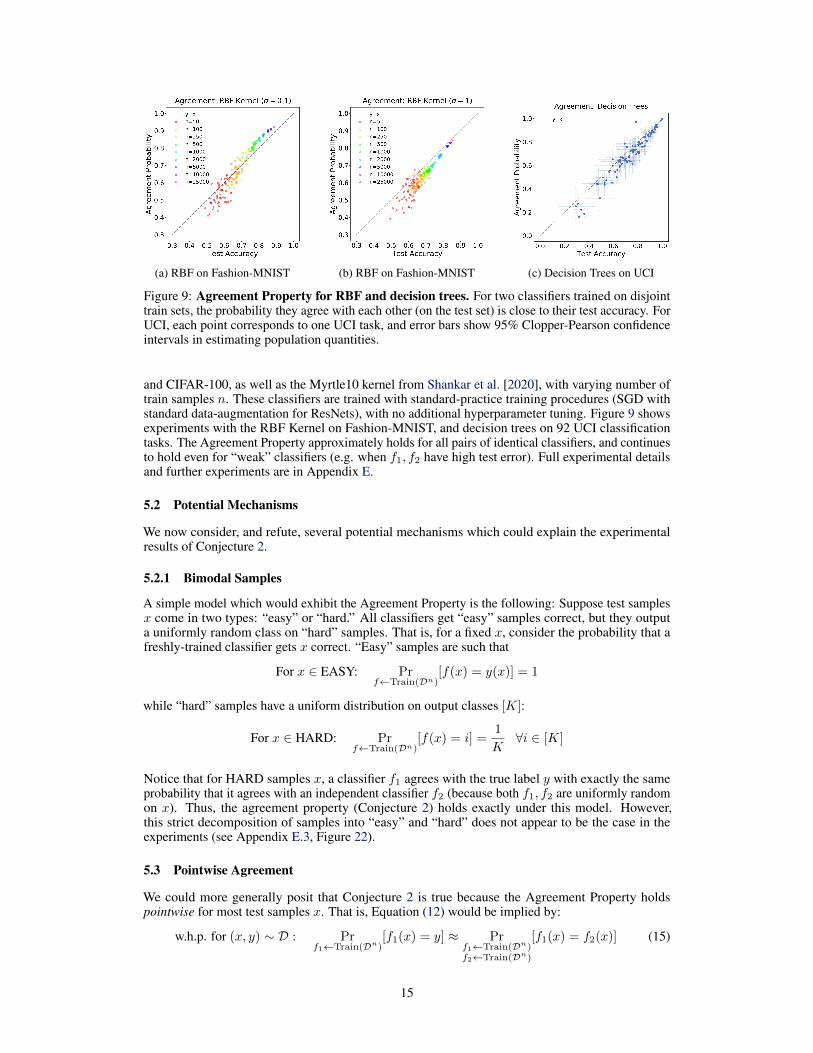
Figure 9: Agreement Property for RBF and decision trees. For two classifiers trained on disjointtrain sets, the probability they agree with each other (on the test set) is close to their test accuracy. ForUCI, each point corresponds to one UCI task, and error bars show 95% Clopper-Pearson confidenceintervals in estimating population quantities.

and CIFAR-100, as well as the Myrtle10 kernel from Shankar et al. [2020], with varying number oftrain samples n. These classifiers are trained with standard-practice training procedures (SGD withstandard data-augmentation for ResNets), with no additional hyperparameter tuning. Figure 9 showsexperiments with the RBF Kernel on Fashion-MNIST, and decision trees on 92 UCI classificationtasks. The Agreement Property approximately holds for all pairs of identical classifiers, and continuesto hold even for “weak” classifiers (e.g. when f1, f2 have high test error). Full experimental detailsand further experiments are in Appendix E.

5.2 Potential Mechanisms

We now consider, and refute, several potential mechanisms which could explain the experimentalresults of Conjecture 2.

5.2.1 Bimodal Samples

A simple model which would exhibit the Agreement Property is the following: Suppose test samplesx come in two types: “easy” or “hard.” All classifiers get “easy” samples correct, but they outputa uniformly random class on “hard” samples. That is, for a fixed x, consider the probability that afreshly-trained classifier gets x correct. “Easy” samples are such that

For x ∈ EASY: Prf←Train(Dn)

[f(x) = y(x)] = 1

while “hard” samples have a uniform distribution on output classes [K]:

For x ∈ HARD: Prf←Train(Dn)

[f(x) = i] =1

K∀i ∈ [K]

Notice that for HARD samples x, a classifier f1 agrees with the true label y with exactly the sameprobability that it agrees with an independent classifier f2 (because both f1, f2 are uniformly randomon x). Thus, the agreement property (Conjecture 2) holds exactly under this model. However,this strict decomposition of samples into “easy” and “hard” does not appear to be the case in theexperiments (see Appendix E.3, Figure 22).

5.3 Pointwise Agreement

We could more generally posit that Conjecture 2 is true because the Agreement Property holdspointwise for most test samples x. That is, Equation (12) would be implied by:

w.h.p. for (x, y) ∼ D : Prf1←Train(Dn)

[f1(x) = y] ≈ Prf1←Train(Dn)f2←Train(Dn)

[f1(x) = f2(x)] (15)

15

This was the case for the EASY/HARD decomposition above, but could be true in more generalsettings. Equation (15) is a “pointwise calibration” property that would allow estimating the probabil-ity of making an error on a test point x by simply estimating the probability that two independentclassifiers agree on x. However, we find (perhaps surprisingly) that this is not the case. That is, Equa-tion (12) holds on average over (x, y) ∼ D, but not pointwise for each sample. We give experimentsdemonstrating this in Appendix E.3. Interestingly, 1-nearest neighbors can satisfy the agreementproperty of Claim 2 without satisfying the “pointwise agreement” of Equation 15. It remains an openproblem to understand the mechanisms behind Agreement Matching.

6 Limitations and Ensembles

The conjectures presented in this work are not fully specified, since they do not exactly specify whichclassifiers or distributions for which they hold. We experimentally demonstrate instances of theseconjectures in various “natural” settings in machine learning, but we do not yet understand whichassumptions on the distribution or classifier are required. Some experiments also deviate slightlyfrom the predicted behavior (e.g. the kernel experiments in Figures 3 and 9). Nevertheless, we believeour conjectures capture the essential aspects of the observed behaviors, at least to first order. It isan important open question to refine these conjectures and better understand their applications andlimitations— both theoretically and experimentally.

6.1 Ensembles

We could ask if all high-performing interpolating methods used in practice satisfy our conjectures.However, an important family of classifiers which fail our Feature Calibration Conjecture are ensemblemethods:

1. Deep ensembles of interpolating neural networks [Lakshminarayanan et al., 2017].

2. Random forests (i.e. ensembles of interpolating decision trees) [Breiman, 2001].

3. k-nearest neighbors (roughly “ensembles” of 1-Nearest-Neighbors) [Fix and Hodges, 1951].

The pointwise density estimation discussion in Section 4.6 sheds some light on these cases. Noticethat these are settings where the “base” classifier in the ensemble obeys Feature Calibration, and inparticular, acts as an approximate conditional density estimator of p(y|x), as in Section 4.6. That is,if individual base classifiers fi approximately act as samples from

fi(x) ∼ p(y|x)

then for sufficiently many classifiers {f1, . . . , fk} trained on independent train sets, the ensembledclassifier will act as

plurality(f1, f2, . . . , fk)(x) ≈ argmaxy

p(y|x)

Thus, we believe ensembles fail our conjectures because, in taking the plurality vote of base classifiers,they are approximating argmaxy p(y|x) instead of the conditional density p(y|x) itself. Indeed, inthe above examples, we observed that ensemble methods behave much closer to the Bayes-optimalclassifier than their underlying base classifiers (especially in settings with label noise).

7 Distributional Generalization: Beyond Interpolating Methods

The previous sections have focused primarily on interpolating classifiers, which fit their train setsexactly. Here we discuss the behavior of non-interpolating methods, such as early-stopped neuralnetworks and regularized kernel machines, which do not reach 0 train error.

For non-interpolating classifiers, their outputs on the train set (x, f(x))x∼TrainSet will not match theoriginal distribution (x, y) ∼ D. Thus, there is little hope that their outputs on the test set will matchthe original distribution, and we do not expect the Indistinguishability Conjecture to hold. However,the Distributional Generalization framework does not require interpolation, and we could still expectthat the train and test distributions are close (Dtr ≈T Dte) for some family of tests T . For example,the following is a possible generalization of Feature Calibration (Conjecture 1).

16

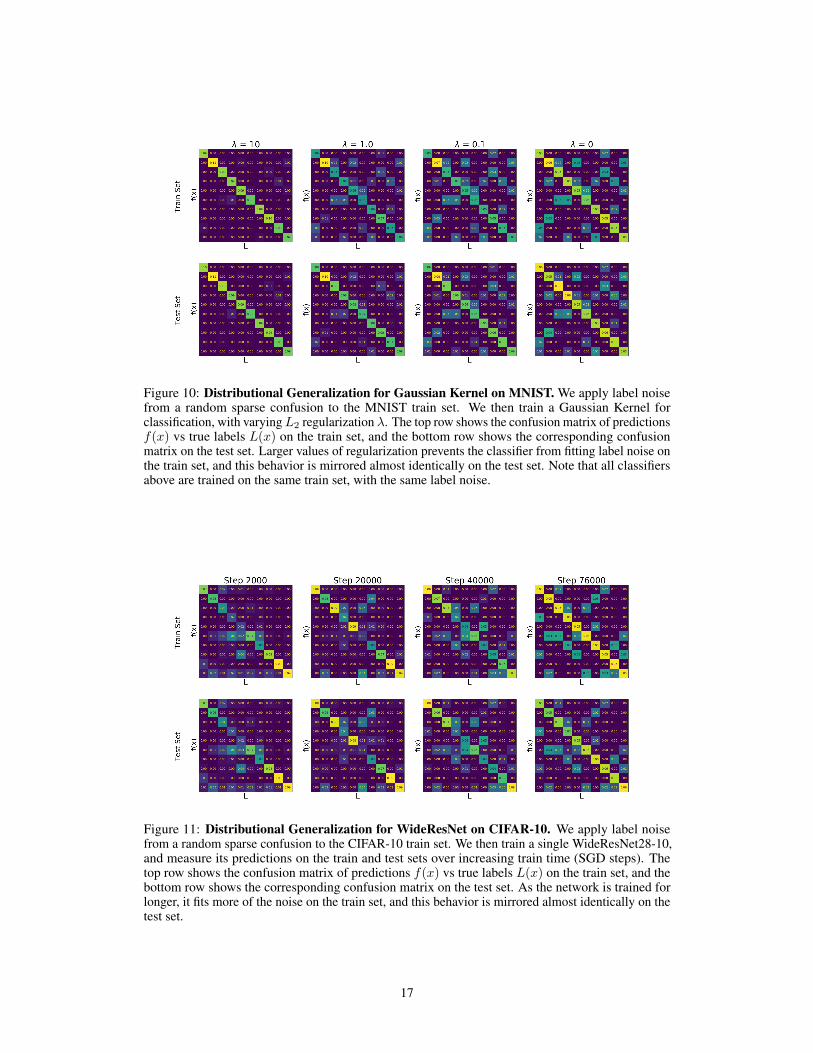
Figure 10: Distributional Generalization for Gaussian Kernel on MNIST. We apply label noisefrom a random sparse confusion to the MNIST train set. We then train a Gaussian Kernel forclassification, with varyingL2 regularization λ. The top row shows the confusion matrix of predictionsf(x) vs true labels L(x) on the train set, and the bottom row shows the corresponding confusionmatrix on the test set. Larger values of regularization prevents the classifier from fitting label noise onthe train set, and this behavior is mirrored almost identically on the test set. Note that all classifiersabove are trained on the same train set, with the same label noise.

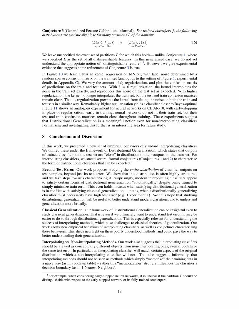
Figure 11: Distributional Generalization for WideResNet on CIFAR-10. We apply label noisefrom a random sparse confusion to the CIFAR-10 train set. We then train a single WideResNet28-10,and measure its predictions on the train and test sets over increasing train time (SGD steps). Thetop row shows the confusion matrix of predictions f(x) vs true labels L(x) on the train set, and thebottom row shows the corresponding confusion matrix on the test set. As the network is trained forlonger, it fits more of the noise on the train set, and this behavior is mirrored almost identically on thetest set.

17

Conjecture 3 (Generalized Feature Calibration, informal). For trained classifiers f , the followingdistributions are statistically close for many partitions L of the domain:

(L(xi), f(xi))xi∼TrainSet

≈ (L(x), f(x))x∼TestSet

(16)

We leave unspecified the exact set of partitions L for which this holds— unlike Conjecture 1, wherewe specified L as the set of all distinguishable features. In this generalized case, we do not yetunderstand the appropriate notion of “distinguishable feature” 5. However, we give experimentalevidence that suggests some refinement of Conjecture 3 is true.

In Figure 10 we train Gaussian kernel regression on MNIST, with label noise determined by arandom sparse confusion matrix on the train set (analogous to the setting of Figure 5; experimentaldetails in Appendix C). We vary the amount of `2 regularization, and plot the confusion matrixof predictions on the train and test sets. With λ = 0 regularization, the kernel interpolates thenoise in the train set exactly, and reproduces this noise on the test set as expected. With higherregularization, the kernel no longer interpolates the train set, but the test and train confusion matricesremain close. That is, regularization prevents the kernel from fitting the noise on both the train andtest sets in a similar way. Remarkably, higher regularization yields a classifier closer to Bayes-optimal.Figure 11 shows an analogous experiment for neural networks on CIFAR-10, with early-stoppingin place of regularization: early in training, neural networks do not fit their train set, but theirtest and train confusion matrices remain close throughout training. These experiments suggestthat Distributional Generalization is a meaningful notion even for non-interpolating classifiers.Formalizing and investigating this further is an interesting area for future study.

8 Conclusion and Discussion

In this work, we presented a new set of empirical behaviors of standard interpolating classifiers.We unified these under the framework of Distributional Generalization, which states that outputsof trained classifiers on the test set are “close” in distribution to their outputs on the train set. Forinterpolating classifiers, we stated several formal conjectures (Conjectures 1 and 2) to characterizethe form of distributional closeness that can be expected.

Beyond Test Error. Our work proposes studying the entire distribution of classifier outputs ontest samples, beyond just its test error. We show that this distribution is often highly structured,and we take steps towards characterizing it. Surprisingly, modern interpolating classifiers appearto satisfy certain forms of distributional generalization “automatically,” despite being trained tosimply minimize train error. This even holds in cases when satisfying distributional generalizationis in conflict with satisfying classical generalization— that is, when a distributionally-generalizingclassifier must necessarily have high test error (e.g. Experiment 1). We thus hope that studyingdistributional generalization will be useful to better understand modern classifiers, and to understandgeneralization more broadly.

Classical Generalization. Our framework of Distributional Generalization can be insightful even tostudy classical generalization. That is, even if we ultimately want to understand test error, it may beeasier to do so through distributional generalization. This is especially relevant for understanding thesuccess of interpolating methods, which pose challenges to classical theories of generalization. Ourwork shows new empirical behaviors of interpolating classifiers, as well as conjectures characterizingthese behaviors. This sheds new light on these poorly understood methods, and could pave the way tobetter understanding their generalization.

Interpolating vs. Non-interpolating Methods. Our work also suggests that interpolating classifiersshould be viewed as conceptually different objects from non-interpolating ones, even if both havethe same test error. In particular, an interpolating classifier will match certain aspects of the originaldistribution, which a non-interpolating classifier will not. This also suggests, informally, thatinterpolating methods should not be seen as methods which simply “memorize” their training data ina naive way (as in a look up table) – rather this “memorization” strongly influences the classifier’sdecision boundary (as in 1-Nearest-Neighbors).

5For example, when considering early-stopped neural networks, it is unclear if the partition L should bedistinguishable with respect to the early-stopped network or its fully-trained counterpart.

18

8.1 Open Questions

Our work raises a number of open questions and connections to other areas. We briefly collect someof them here.

1. As described in the Limitations (Section 6), we do not precisely understand the set ofdistributions and interpolating classifiers for which our conjectures hold. We empiricallytested a number of “realistic” settings, but it is open to state formal assumptions definingthese settings.

2. It is open to theoretically prove versions of Distributional Generalization for models beyond1-Nearest-Neighbors. This is most interesting in cases where Distributional Generalizationis at odds with classical generalization (e.g. Figure 4c).

3. It is open to understand the mechanisms behind the Agreement Property (Section 5), theo-retically or empirically.

4. In some of our experiments (e.g. Section 4.6), ensembling over independent random-initializations had a similar effect to ensembling over independent train sets. This is relatedto works on deep ensembles [Fort et al., 2019a, Lakshminarayanan et al., 2017] as well asrandom forests for conditional density estimation [Athey et al., 2019, Meinshausen, 2006,Pospisil and Lee, 2018]. Investigating this further is an interesting area of future work.

5. There are a number of works suggesting “local” behavior of neural networks, and theseare somewhat consistent with our locality intuitions in this work. However, it is open toformally understand whether these intuitions are justified in our setting.

6. We give two families of tests T for which our Interpolating Indistinguishability conjecture(Equation 3) empirically holds. This may not be exhaustive – there may be other waysin which the source distribution D and test distribution Dte are close. Indeed, we givepreliminary experiments for another family of tests, based on student-teacher training, inAppendix B. It is open to explore more ways in which Distributional Generalization holds,beyond the tests presented here.

Acknowledgements

We especially thank Jacob Steinhardt and Boaz Barak for useful discussions during this work. Wethank Vaishaal Shankar for providing the Myrtle10 kernel, the ImageNet classifiers, and adviceregarding UCI tasks. We thank Guy Gur-Ari for noting the connection to existing work on networkspicking up fine-structural aspects of distributions. We also thank a number of people for reviewingearly drafts or providing valuable comments, including: Collin Burns, Mihaela Curmei, BenjaminL. Edelman, Sara Fridovich-Keil, Boriana Gjura, Wenshuo Guo, Thibaut Horel, Meena Jagadeesan,Dimitris Kalimeris, Gal Kaplun, Song Mei, Aditi Raghunathan, Ludwig Schmidt, Ilya Sutskever,Yaodong Yu, Kelly W. Zhang, Ruiqi Zhong.

Work supported in part by the Simons Investigator Awards of Boaz Barak and Madhu Sudan, andNSF Awards under grants CCF 1565264, CCF 1715187 and IIS 1409097. Computational resourcessupported in part by a gift from Oracle, and Microsoft Azure credits (via Harvard Data ScienceInitiative). P.N. supported in part by a Google PhD Fellowship. Y.B is partially supported byMIT-IBM Watson AI Lab.

Technologies. This work was built on the following technologies: NumPy [Harris et al., 2020,Oliphant, 2006, Van Der Walt et al., 2011], SciPy [Virtanen et al., 2020], scikit-learn [Pedregosaet al., 2011], PyTorch [Paszke et al., 2019], W&B [Biewald, 2020], Matplotlib [Hunter, 2007], pandas[pandas development team, 2020, Wes McKinney, 2010], SLURM [Yoo et al., 2003], Figma. Neuralnetworks trained on NVIDIA V100 and 2080 Ti GPUs.

19

ReferencesMadhu S Advani and Andrew M Saxe. High-dimensional dynamics of generalization error in neural

networks. arXiv preprint arXiv:1710.03667, 2017.

Zeyuan Allen-Zhu, Yuanzhi Li, and Yingyu Liang. Learning and generalization in overparameterizedneural networks, going beyond two layers. In Advances in neural information processing systems,pages 6158–6169, 2019.

Sanjeev Arora, Simon Du, Wei Hu, Zhiyuan Li, and Ruosong Wang. Fine-grained analysis ofoptimization and generalization for overparameterized two-layer neural networks. In InternationalConference on Machine Learning, pages 322–332, 2019.

Susan Athey, Julie Tibshirani, Stefan Wager, et al. Generalized random forests. The Annals ofStatistics, 47(2):1148–1178, 2019.

Francis Bach. Breaking the curse of dimensionality with convex neural networks. The Journal ofMachine Learning Research, 18(1):629–681, 2017.

Peter L Bartlett, Philip M Long, Gábor Lugosi, and Alexander Tsigler. Benign overfitting in linearregression. Proceedings of the National Academy of Sciences, 2020.

David Bau, Jun-Yan Zhu, Hendrik Strobelt, Agata Lapedriza, Bolei Zhou, and Antonio Torralba.Understanding the role of individual units in a deep neural network. Proceedings of the NationalAcademy of Sciences, 2020.

Mikhail Belkin, Daniel J Hsu, and Partha Mitra. Overfitting or perfect fitting? risk bounds forclassification and regression rules that interpolate. In Advances in neural information processingsystems, pages 2300–2311, 2018a.

Mikhail Belkin, Siyuan Ma, and Soumik Mandal. To understand deep learning we need to understandkernel learning. arXiv preprint arXiv:1802.01396, 2018b.

Mikhail Belkin, Daniel Hsu, Siyuan Ma, and Soumik Mandal. Reconciling modern machine-learningpractice and the classical bias–variance trade-off. Proceedings of the National Academy of Sciences,116(32):15849–15854, 2019.

Lukas Biewald. Experiment tracking with weights and biases, 2020. URL https://www.wandb.com/. Software available from wandb.com.

Leo Breiman. Reflections after refereeing papers for nips. The Mathematics of Generalization, pages11–15, 1995.

Leo Breiman. Random forests. Machine learning, 45(1):5–32, 2001.

Leo Breiman, Jerome Friedman, Charles J Stone, and Richard A Olshen. Classification and regressiontrees. CRC press, 1984.

Nick Cammarata, Shan Carter, Gabriel Goh, Chris Olah, Michael Petrov, and Ludwig Schubert.Thread: Circuits. Distill, 2020. doi: 10.23915/distill.00024. https://distill.pub/2020/circuits.

Shan Carter, Zan Armstrong, Ludwig Schubert, Ian Johnson, and Chris Olah. Activation atlas. Distill,4(3):e15, 2019.

Niladri S Chatterji and Philip M Long. Finite-sample analysis of interpolating linear classifiers in theoverparameterized regime. arXiv preprint arXiv:2004.12019, 2020.

Lenaic Chizat and Francis Bach. Implicit bias of gradient descent for wide two-layer neural networkstrained with the logistic loss. arXiv preprint arXiv:2002.04486, 2020.

Dheeru Dua and Casey Graff. UCI machine learning repository, 2017. URL http://archive.ics.uci.edu/ml.

Gintare Karolina Dziugaite and Daniel M Roy. Computing nonvacuous generalization bounds fordeep (stochastic) neural networks with many more parameters than training data. arXiv preprintarXiv:1703.11008, 2017.

20

Manuel Fernández-Delgado, Eva Cernadas, Senén Barro, and Dinani Amorim. Do we need hundredsof classifiers to solve real world classification problems? The journal of machine learning research,15(1):3133–3181, 2014.

Evelyn Fix and JL Hodges. Discriminatory analysis: nonparametric discrimination, consistencyproperties. USAF School of Aviation Medicine, 1951.

Stanislav Fort, Huiyi Hu, and Balaji Lakshminarayanan. Deep ensembles: A loss landscape perspec-tive. arXiv preprint arXiv:1912.02757, 2019a.

Stanislav Fort, Paweł Krzysztof Nowak, Stanislaw Jastrzebski, and Srini Narayanan. Stiffness: Anew perspective on generalization in neural networks. arXiv preprint arXiv:1901.09491, 2019b.

Mario Geiger, Stefano Spigler, Stéphane d’Ascoli, Levent Sagun, Marco Baity-Jesi, Giulio Biroli,and Matthieu Wyart. Jamming transition as a paradigm to understand the loss landscape of deepneural networks. Physical Review E, 100(1):012115, 2019.

Federica Gerace, Bruno Loureiro, Florent Krzakala, Marc Mézard, and Lenka Zdeborová. Gener-alisation error in learning with random features and the hidden manifold model. arXiv preprintarXiv:2002.09339, 2020.

Behrooz Ghorbani, Song Mei, Theodor Misiakiewicz, and Andrea Montanari. Linearized two-layersneural networks in high dimension. arXiv preprint arXiv:1904.12191, 2019.

Dar Gilboa and Guy Gur-Ari. Wider networks learn better features. arXiv preprint arXiv:1909.11572,2019.

Tilmann Gneiting and Adrian E Raftery. Strictly proper scoring rules, prediction, and estimation.Journal of the American statistical Association, 102(477):359–378, 2007.

Sebastian Goldt, Madhu S Advani, Andrew M Saxe, Florent Krzakala, and Lenka Zdeborova.Generalisation dynamics of online learning in over-parameterised neural networks. arXiv preprintarXiv:1901.09085, 2019.

Chuan Guo, Geoff Pleiss, Yu Sun, and Kilian Q Weinberger. On calibration of modern neuralnetworks. arXiv preprint arXiv:1706.04599, 2017.

Charles R. Harris, K. Jarrod Millman, Stéfan J. van der Walt, Ralf Gommers, Pauli Virtanen,David Cournapeau, Eric Wieser, Julian Taylor, Sebastian Berg, Nathaniel J. Smith, Robert Kern,Matti Picus, Stephan Hoyer, Marten H. van Kerkwijk, Matthew Brett, Allan Haldane, Jaime Fer-nández del Río, Mark Wiebe, Pearu Peterson, Pierre Gérard-Marchant, Kevin Sheppard, TylerReddy, Warren Weckesser, Hameer Abbasi, Christoph Gohlke, and Travis E. Oliphant. Arrayprogramming with numpy. Nature, 585(7825):357–362, Sep 2020. ISSN 1476-4687. doi:10.1038/s41586-020-2649-2. URL https://doi.org/10.1038/s41586-020-2649-2.

Trevor Hastie, Robert Tibshirani, and Jerome Friedman. The elements of statistical learning: datamining, inference, and prediction. Springer Science & Business Media, 2009.

Trevor Hastie, Andrea Montanari, Saharon Rosset, and Ryan J Tibshirani. Surprises in high-dimensional ridgeless least squares interpolation. arXiv preprint arXiv:1903.08560, 2019.

Kaiming He, Xiangyu Zhang, Shaoqing Ren, and Jian Sun. Deep residual learning for imagerecognition. In Proceedings of the IEEE conference on computer vision and pattern recognition,pages 770–778, 2016.

Úrsula Hébert-Johnson, Michael Kim, Omer Reingold, and Guy Rothblum. Multicalibration: Cali-bration for the (computationally-identifiable) masses. In International Conference on MachineLearning, pages 1939–1948, 2018.

Tin Kam Ho. Random decision forests. In Proceedings of 3rd international conference on documentanalysis and recognition, volume 1, pages 278–282. IEEE, 1995.

J. D. Hunter. Matplotlib: A 2d graphics environment. Computing in Science & Engineering, 9(3):90–95, 2007. doi: 10.1109/MCSE.2007.55.

21

Rashidedin Jahandideh, Alireza Tavakoli Targhi, and Maryam Tahmasbi. Physical attribute predictionusing deep residual neural networks. arXiv preprint arXiv:1812.07857, 2018.

Ziwei Ji and Matus Telgarsky. Polylogarithmic width suffices for gradient descent to achievearbitrarily small test error with shallow relu networks. arXiv preprint arXiv:1909.12292, 2019.

Alex Krizhevsky et al. Learning multiple layers of features from tiny images. 2009.

Balaji Lakshminarayanan, Alexander Pritzel, and Charles Blundell. Simple and scalable predictiveuncertainty estimation using deep ensembles. In Advances in neural information processingsystems, pages 6402–6413, 2017.

Yann LeCun, Léon Bottou, Yoshua Bengio, and Patrick Haffner. Gradient-based learning applied todocument recognition. Proceedings of the IEEE, 86(11):2278–2324, 1998.

Tengyuan Liang and Alexander Rakhlin. Just interpolate: Kernel" ridgeless" regression can generalize.arXiv preprint arXiv:1808.00387, 2018.

Ziwei Liu, Ping Luo, Xiaogang Wang, and Xiaoou Tang. Deep learning face attributes in the wild. InProceedings of International Conference on Computer Vision (ICCV), December 2015.

Song Mei and Andrea Montanari. The generalization error of random features regression: Preciseasymptotics and double descent curve. arXiv preprint arXiv:1908.05355, 2019.

Nicolai Meinshausen. Quantile regression forests. Journal of Machine Learning Research, 7(Jun):983–999, 2006.

Alfred Müller. Integral probability metrics and their generating classes of functions. Advances inApplied Probability, 29(2):429–443, 1997.

Vidya Muthukumar, Kailas Vodrahalli, Vignesh Subramanian, and Anant Sahai. Harmless inter-polation of noisy data in regression. IEEE Journal on Selected Areas in Information Theory,2020.

Elizbar A Nadaraya. On estimating regression. Theory of Probability & Its Applications, 9(1):141–142, 1964.

Vaishnavh Nagarajan and J. Zico Kolter. Uniform convergence may be unable to explain generaliza-tion in deep learning, 2019.

Preetum Nakkiran, Gal Kaplun, Yamini Bansal, Tristan Yang, Boaz Barak, and Ilya Sutskever. Deepdouble descent: Where bigger models and more data hurt. In International Conference on LearningRepresentations, 2020.

Hariharan Narayanan and Sanjoy Mitter. Sample complexity of testing the manifold hypothesis. InAdvances in neural information processing systems, pages 1786–1794, 2010.

Nagarajan Natarajan, Inderjit S Dhillon, Pradeep K Ravikumar, and Ambuj Tewari. Learning withnoisy labels. In Advances in neural information processing systems, pages 1196–1204, 2013.

Brady Neal, Sarthak Mittal, Aristide Baratin, Vinayak Tantia, Matthew Scicluna, Simon Lacoste-Julien, and Ioannis Mitliagkas. A modern take on the bias-variance tradeoff in neural networks.arXiv preprint arXiv:1810.08591, 2018.

Behnam Neyshabur, Zhiyuan Li, Srinadh Bhojanapalli, Yann LeCun, and Nathan Srebro. Towardsunderstanding the role of over-parametrization in generalization of neural networks. arXiv preprintarXiv:1805.12076, 2018.

Alexandru Niculescu-Mizil and Rich Caruana. Predicting good probabilities with supervised learning.In Proceedings of the 22nd international conference on Machine learning, pages 625–632, 2005.

Chris Olah, Arvind Satyanarayan, Ian Johnson, Shan Carter, Ludwig Schubert, Katherine Ye, andAlexander Mordvintsev. The building blocks of interpretability. Distill, 3(3):e10, 2018.

Travis E Oliphant. A guide to NumPy, volume 1. Trelgol Publishing USA, 2006.

22

Matthew A Olson and Abraham J Wyner. Making sense of random forest probabilities: a kernelperspective. arXiv preprint arXiv:1812.05792, 2018.

The pandas development team. pandas-dev/pandas: Pandas, February 2020. URL https://doi.org/10.5281/zenodo.3509134.

Adam Paszke, Sam Gross, Soumith Chintala, Gregory Chanan, Edward Yang, Zachary DeVito,Zeming Lin, Alban Desmaison, Luca Antiga, and Adam Lerer. Automatic differentiation inpytorch. 2017.

Adam Paszke, Sam Gross, Francisco Massa, Adam Lerer, James Bradbury, Gregory Chanan,Trevor Killeen, Zeming Lin, Natalia Gimelshein, Luca Antiga, Alban Desmaison, AndreasKopf, Edward Yang, Zachary DeVito, Martin Raison, Alykhan Tejani, Sasank Chilamkurthy,Benoit Steiner, Lu Fang, Junjie Bai, and Soumith Chintala. Pytorch: An imperative style,high-performance deep learning library. In H. Wallach, H. Larochelle, A. Beygelzimer, F. dÁlché-Buc, E. Fox, and R. Garnett, editors, Advances in Neural Information Processing Systems 32,pages 8026–8037. Curran Associates, Inc., 2019. URL http://papers.nips.cc/paper/9015-pytorch-an-imperative-style-high-performance-deep-learning-library.pdf.

F. Pedregosa, G. Varoquaux, A. Gramfort, V. Michel, B. Thirion, O. Grisel, M. Blondel, P. Pretten-hofer, R. Weiss, V. Dubourg, J. Vanderplas, A. Passos, D. Cournapeau, M. Brucher, M. Perrot, andE. Duchesnay. Scikit-learn: Machine learning in Python. Journal of Machine Learning Research,12:2825–2830, 2011.

Taylor Pospisil and Ann B Lee. Rfcde: Random forests for conditional density estimation. arXivpreprint arXiv:1804.05753, 2018.

Alec Radford, Rafal Jozefowicz, and Ilya Sutskever. Learning to generate reviews and discoveringsentiment. arXiv preprint arXiv:1704.01444, 2017.

Ali Rahimi and Benjamin Recht. Random features for large-scale kernel machines. In Advances inneural information processing systems, pages 1177–1184, 2008.

David Rolnick, Andreas Veit, Serge Belongie, and Nir Shavit. Deep learning is robust to massivelabel noise. arXiv preprint arXiv:1705.10694, 2017.

Jonas Rothfuss, Fabio Ferreira, Simon Walther, and Maxim Ulrich. Conditional density estimationwith neural networks: Best practices and benchmarks. arXiv preprint arXiv:1903.00954, 2019.

Olga Russakovsky, Jia Deng, Hao Su, Jonathan Krause, Sanjeev Satheesh, Sean Ma, Zhiheng Huang,Andrej Karpathy, Aditya Khosla, Michael Bernstein, Alexander C. Berg, and Li Fei-Fei. ImageNetLarge Scale Visual Recognition Challenge. International Journal of Computer Vision (IJCV), 115(3):211–252, 2015. doi: 10.1007/s11263-015-0816-y.

Robert E Schapire. Theoretical views of boosting. In European conference on computational learningtheory, pages 1–10. Springer, 1999.

Robert E Schapire, Yoav Freund, Peter Bartlett, Wee Sun Lee, et al. Boosting the margin: A newexplanation for the effectiveness of voting methods. The annals of statistics, 26(5):1651–1686,1998.

Vaishaal Shankar, Alex Fang, Wenshuo Guo, Sara Fridovich-Keil, Ludwig Schmidt, Jonathan Ragan-Kelley, and Benjamin Recht. Neural kernels without tangents. arXiv preprint arXiv:2003.02237,2020.

Utkarsh Sharma and Jared Kaplan. A neural scaling law from the dimension of the data manifold.arXiv preprint arXiv:2004.10802, 2020.

Daniel Soudry, Elad Hoffer, Mor Shpigel Nacson, Suriya Gunasekar, and Nathan Srebro. The implicitbias of gradient descent on separable data. The Journal of Machine Learning Research, 19(1):2822–2878, 2018.

23

Sunil Thulasidasan, Tanmoy Bhattacharya, Jeff Bilmes, Gopinath Chennupati, and Jamal Mohd-Yusof. Combating label noise in deep learning using abstention. arXiv preprint arXiv:1905.10964,2019.

Alexandre B Tsybakov. Introduction to nonparametric estimation. Springer Science & BusinessMedia, 2008.

Stefan Van Der Walt, S Chris Colbert, and Gael Varoquaux. The numpy array: a structure for efficientnumerical computation. Computing in Science & Engineering, 13(2):22, 2011.

Pauli Virtanen, Ralf Gommers, Travis E. Oliphant, Matt Haberland, Tyler Reddy, David Cournapeau,Evgeni Burovski, Pearu Peterson, Warren Weckesser, Jonathan Bright, Stéfan J. van der Walt,Matthew Brett, Joshua Wilson, K. Jarrod Millman, Nikolay Mayorov, Andrew R. J. Nelson, EricJones, Robert Kern, Eric Larson, CJ Carey, Ilhan Polat, Yu Feng, Eric W. Moore, Jake Vand erPlas,Denis Laxalde, Josef Perktold, Robert Cimrman, Ian Henriksen, E. A. Quintero, Charles R Harris,Anne M. Archibald, Antônio H. Ribeiro, Fabian Pedregosa, Paul van Mulbregt, and SciPy 1. 0Contributors. SciPy 1.0: Fundamental Algorithms for Scientific Computing in Python. NatureMethods, 17:261–272, 2020. doi: https://doi.org/10.1038/s41592-019-0686-2.

Larry Wasserman. All of nonparametric statistics. Springer Science & Business Media, 2006.

Geoffrey S Watson. Smooth regression analysis. Sankhya: The Indian Journal of Statistics, Series A,pages 359–372, 1964.

Wes McKinney. Data Structures for Statistical Computing in Python. In Stéfan van der Walt andJarrod Millman, editors, Proceedings of the 9th Python in Science Conference, pages 56 – 61, 2010.doi: 10.25080/Majora-92bf1922-00a.

Abraham J Wyner, Matthew Olson, Justin Bleich, and David Mease. Explaining the success ofadaboost and random forests as interpolating classifiers. The Journal of Machine LearningResearch, 18(1):1558–1590, 2017.

Han Xiao, Kashif Rasul, and Roland Vollgraf. Fashion-mnist: a novel image dataset for benchmarkingmachine learning algorithms. arXiv preprint arXiv:1708.07747, 2017.

Mohammad Yaghini, Bogdan Kulynych, and Carmela Troncoso. Disparate vulnerability: On theunfairness of privacy attacks against machine learning. arXiv preprint arXiv:1906.00389, 2019.

Andy B Yoo, Morris A Jette, and Mark Grondona. Slurm: Simple linux utility for resource manage-ment. In Workshop on Job Scheduling Strategies for Parallel Processing, pages 44–60. Springer,2003.

Sergey Zagoruyko and Nikos Komodakis. Wide residual networks. arXiv preprint arXiv:1605.07146,2016.

Chiyuan Zhang, Samy Bengio, Moritz Hardt, Benjamin Recht, and Oriol Vinyals. Understandingdeep learning requires rethinking generalization. arXiv preprint arXiv:1611.03530, 2016.

Bolei Zhou, Aditya Khosla, Agata Lapedriza, Aude Oliva, and Antonio Torralba. Object detectorsemerge in deep scene cnns. arXiv preprint arXiv:1412.6856, 2014.

Liu Ziyin, Blair Chen, Ru Wang, Paul Pu Liang, Ruslan Salakhutdinov, Louis-Philippe Morency,and Masahito Ueda. Learning not to learn in the presence of noisy labels. arXiv preprintarXiv:2002.06541, 2020.

24

A Author Contributions

PN designed the initial neural network experiments which initiated this study. PN and YB brain-stormed the formalization of the experimental observations and PN devised the final version of thedefinitions, conjectures, and their framing as a version of generalization. YB designed the exper-iments to stress test the Feature Calibration Conjecture under various settings and conducted thefinal experiments that appear in the Feature Calibration section. PN discovered and investigatedthe Agreement Property and did the Student-Teacher section. PN did the kernel and decision treeexperiments, literature review, and nearest-neighbor proofs. Both authors wrote the paper.

25

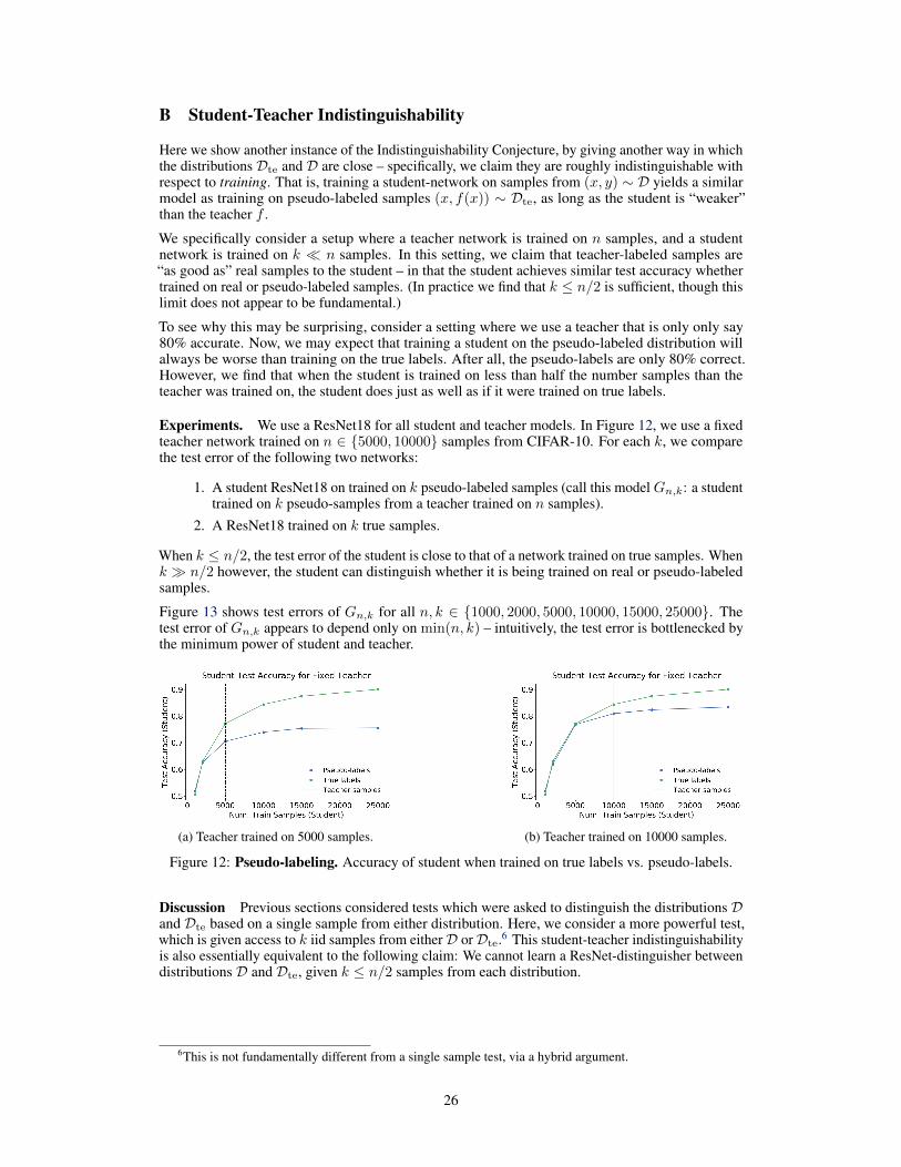
B Student-Teacher Indistinguishability

Here we show another instance of the Indistinguishability Conjecture, by giving another way in whichthe distributions Dte and D are close – specifically, we claim they are roughly indistinguishable withrespect to training. That is, training a student-network on samples from (x, y) ∼ D yields a similarmodel as training on pseudo-labeled samples (x, f(x)) ∼ Dte, as long as the student is “weaker”than the teacher f .

We specifically consider a setup where a teacher network is trained on n samples, and a studentnetwork is trained on k � n samples. In this setting, we claim that teacher-labeled samples are“as good as” real samples to the student – in that the student achieves similar test accuracy whethertrained on real or pseudo-labeled samples. (In practice we find that k ≤ n/2 is sufficient, though thislimit does not appear to be fundamental.)

To see why this may be surprising, consider a setting where we use a teacher that is only only say80% accurate. Now, we may expect that training a student on the pseudo-labeled distribution willalways be worse than training on the true labels. After all, the pseudo-labels are only 80% correct.However, we find that when the student is trained on less than half the number samples than theteacher was trained on, the student does just as well as if it were trained on true labels.

Experiments. We use a ResNet18 for all student and teacher models. In Figure 12, we use a fixedteacher network trained on n ∈ {5000, 10000} samples from CIFAR-10. For each k, we comparethe test error of the following two networks:

1. A student ResNet18 on trained on k pseudo-labeled samples (call this model Gn,k: a studenttrained on k pseudo-samples from a teacher trained on n samples).

2. A ResNet18 trained on k true samples.

When k ≤ n/2, the test error of the student is close to that of a network trained on true samples. Whenk � n/2 however, the student can distinguish whether it is being trained on real or pseudo-labeledsamples.

Figure 13 shows test errors of Gn,k for all n, k ∈ {1000, 2000, 5000, 10000, 15000, 25000}. Thetest error of Gn,k appears to depend only on min(n, k) – intuitively, the test error is bottlenecked bythe minimum power of student and teacher.

(a) Teacher trained on 5000 samples. (b) Teacher trained on 10000 samples.

Figure 12: Pseudo-labeling. Accuracy of student when trained on true labels vs. pseudo-labels.

Discussion Previous sections considered tests which were asked to distinguish the distributions Dand Dte based on a single sample from either distribution. Here, we consider a more powerful test,which is given access to k iid samples from eitherD orDte.6 This student-teacher indistinguishabilityis also essentially equivalent to the following claim: We cannot learn a ResNet-distinguisher betweendistributions D and Dte, given k ≤ n/2 samples from each distribution.

6This is not fundamentally different from a single sample test, via a hybrid argument.

26

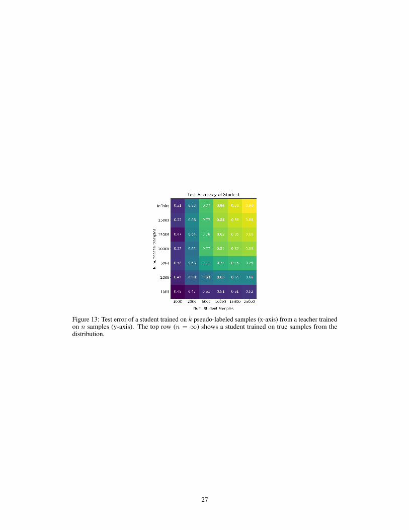
Figure 13: Test error of a student trained on k pseudo-labeled samples (x-axis) from a teacher trainedon n samples (y-axis). The top row (n = ∞) shows a student trained on true samples from thedistribution.

27

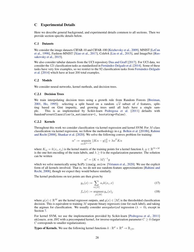
C Experimental Details

Here we describe general background, and experimental details common to all sections. Then weprovide section-specific details below.

C.1 Datasets

We consider the image datasets CIFAR-10 and CIFAR-100 [Krizhevsky et al., 2009], MNIST [LeCunet al., 1998], Fashion-MNIST [Xiao et al., 2017], CelebA [Liu et al., 2015], and ImageNet [Rus-sakovsky et al., 2015].

We also consider tabular datasets from the UCI repository Dua and Graff [2017]. For UCI data, weconsider the 121 classification tasks as standardized in Fernández-Delgado et al. [2014]. Some of thesetasks have very few examples, so we restrict to the 92 classification tasks from Fernández-Delgadoet al. [2014] which have at least 200 total examples.

C.2 Models

We consider neural-networks, kernel methods, and decision trees.

C.2.1 Decision Trees

We train interpolating decision trees using a growth rule from Random Forests [Breiman,2001, Ho, 1995]: selecting a split based on a random

√d subset of d features, split-

ting based on Gini impurity, and growing trees until all leafs have a single sam-ple. This is as implemented by Scikit-learn Pedregosa et al. [2011] defaults withRandomForestClassifier(n_estimators=1, bootstrap=False).

C.2.2 Kernels

Throughout this work we consider classification via kernel regression and kernel SVM. For M -classclassification via kernel regression, we follow the methodology in e.g. Belkin et al. [2018b], Rahimiand Recht [2008], Shankar et al. [2020]. We solve the following convex problem for training:

α∗ := argminα∈RN×M

||Kα− y||22 + λαTKα

where Kij = k(xi, xj) is the kernel matrix of the training points for a kernel function k, y ∈ RN×Mis the one-hot encoding of the train labels, and λ ≥ 0 is the regularization parameter. The solutioncan be written

α∗ = (K + λI)−1y

which we solve numerically using SciPy linalg.solve [Virtanen et al., 2020]. We use the explicitform of all kernels involved. That is, we do not use random-feature approximations [Rahimi andRecht, 2008], though we expect they would behave similarly.

The kernel predictions on test points are then given by

gα(x) :=∑i∈[N ]

αik(xi, x) (17)

fα(x) := argmaxj∈[M ]

gα(x)j (18)

where g(x) ∈ RM are the kernel regressor outputs, and g(x) ∈ [M ] is the thresholded classificationdecision. This is equivalent to training M separate binary regressors (one for each label), and takingthe argmax for classification. We usually consider unregularized regression (λ = 0), except inSection 7.

For kernel SVM, we use the implementation provided by Scikit-learn [Pedregosa et al., 2011]sklearn.svm.SVC with a precomputed kernel, for inverse-regularization parameter C ≥ 0 (largerC corresponds to smaller regularization).

Types of Kernels. We use the following kernel functions k : Rd × Rd → R≥0.

28

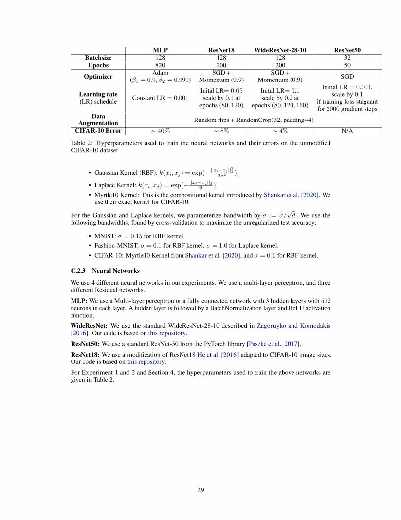
MLP ResNet18 WideResNet-28-10 ResNet50Batchsize 128 128 128 32Epochs 820 200 200 50

Optimizer Adam(β1 = 0.9, β2 = 0.999)

SGD +Momentum (0.9)

SGD +Momentum (0.9) SGD

Learning rate(LR) schedule Constant LR = 0.001

Inital LR= 0.05scale by 0.1 at

epochs (80, 120)

Inital LR= 0.1scale by 0.2 at

epochs (80, 120, 160)

Initial LR = 0.001,scale by 0.1

if training loss stagnantfor 2000 gradient steps

DataAugmentation Random flips + RandomCrop(32, padding=4)

CIFAR-10 Error ∼ 40% ∼ 8% ∼ 4% N/A

Table 2: Hyperparameters used to train the neural networks and their errors on the unmodifiedCIFAR-10 dataset

• Gaussian Kernel (RBF): k(xi, xj) = exp(− ||xi−xj ||222σ2 ).

• Laplace Kernel: k(xi, xj) = exp(− ||xi−xj ||2σ ).

• Myrtle10 Kernel: This is the compositional kernel introduced by Shankar et al. [2020]. Weuse their exact kernel for CIFAR-10.

For the Gaussian and Laplace kernels, we parameterize bandwidth by σ := σ/√d. We use the

following bandwidths, found by cross-validation to maximize the unregularized test accuracy:

• MNIST: σ = 0.15 for RBF kernel.• Fashion-MNIST: σ = 0.1 for RBF kernel. σ = 1.0 for Laplace kernel.• CIFAR-10: Myrtle10 Kernel from Shankar et al. [2020], and σ = 0.1 for RBF kernel.

C.2.3 Neural Networks

We use 4 different neural networks in our experiments. We use a multi-layer perceptron, and threedifferent Residual networks.

MLP: We use a Multi-layer perceptron or a fully connected network with 3 hidden layers with 512neurons in each layer. A hidden layer is followed by a BatchNormalization layer and ReLU activationfunction.

WideResNet: We use the standard WideResNet-28-10 described in Zagoruyko and Komodakis[2016]. Our code is based on this repository.

ResNet50: We use a standard ResNet-50 from the PyTorch library [Paszke et al., 2017].

ResNet18: We use a modification of ResNet18 He et al. [2016] adapted to CIFAR-10 image sizes.Our code is based on this repository.

For Experiment 1 and 2 and Section 4, the hyperparameters used to train the above networks aregiven in Table 2.

29

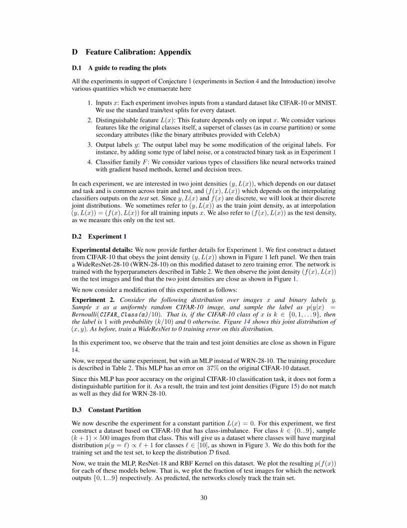
D Feature Calibration: Appendix

D.1 A guide to reading the plots

All the experiments in support of Conjecture 1 (experiments in Section 4 and the Introduction) involvevarious quantities which we enumaerate here

1. Inputs x: Each experiment involves inputs from a standard dataset like CIFAR-10 or MNIST.We use the standard train/test splits for every dataset.

2. Distinguishable feature L(x): This feature depends only on input x. We consider variousfeatures like the original classes itself, a superset of classes (as in coarse partition) or somesecondary attributes (like the binary attributes provided with CelebA)

3. Output labels y: The output label may be some modification of the original labels. Forinstance, by adding some type of label noise, or a constructed binary task as in Experiment 1

4. Classifier family F : We consider various types of classifiers like neural networks trainedwith gradient based methods, kernel and decision trees.

In each experiment, we are interested in two joint densities (y, L(x)), which depends on our datasetand task and is common across train and test, and (f(x), L(x)) which depends on the interpolatingclassifiers outputs on the test set. Since y, L(x) and f(x) are discrete, we will look at their discretejoint distributions. We sometimes refer to (y, L(x)) as the train joint density, as at interpolation(y, L(x)) = (f(x), L(x)) for all training inputs x. We also refer to (f(x), L(x)) as the test density,as we measure this only on the test set.

D.2 Experiment 1

Experimental details: We now provide further details for Experiment 1. We first construct a datasetfrom CIFAR-10 that obeys the joint density (y, L(x)) shown in Figure 1 left panel. We then traina WideResNet-28-10 (WRN-28-10) on this modified dataset to zero training error. The network istrained with the hyperparameters described in Table 2. We then observe the joint density (f(x), L(x))on the test images and find that the two joint densities are close as shown in Figure 1.

We now consider a modification of this experiment as follows:Experiment 2. Consider the following distribution over images x and binary labels y.Sample x as a uniformly random CIFAR-10 image, and sample the label as p(y|x) =Bernoulli(CIFAR_Class(x)/10). That is, if the CIFAR-10 class of x is k ∈ {0, 1, . . . 9}, thenthe label is 1 with probability (k/10) and 0 otherwise. Figure 14 shows this joint distribution of(x, y). As before, train a WideResNet to 0 training error on this distribution.

In this experiment too, we observe that the train and test joint densities are close as shown in Figure14.

Now, we repeat the same experiment, but with an MLP instead of WRN-28-10. The training procedureis described in Table 2. This MLP has an error on 37% on the original CIFAR-10 dataset.

Since this MLP has poor accuracy on the original CIFAR-10 classification task, it does not form adistinguishable partition for it. As a result, the train and test joint densities (Figure 15) do not matchas well as they did for WRN-28-10.

D.3 Constant Partition

We now describe the experiment for a constant partition L(x) = 0. For this experiment, we firstconstruct a dataset based on CIFAR-10 that has class-imbalance. For class k ∈ {0...9}, sample(k + 1)× 500 images from that class. This will give us a dataset where classes will have marginaldistribution p(y = `) ∝ ` + 1 for classes ` ∈ [10], as shown in Figure 3. We do this both for thetraining set and the test set, to keep the distribution D fixed.

Now, we train the MLP, ResNet-18 and RBF Kernel on this dataset. We plot the resulting p(f(x))for each of these models below. That is, we plot the fraction of test images for which the networkoutputs {0, 1...9} respectively. As predicted, the networks closely track the train set.

30

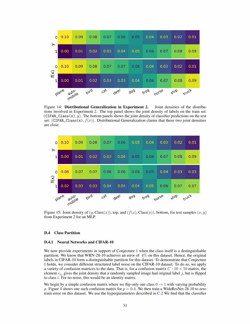
Figure 14: Distributional Generalization in Experiment 2. Joint densities of the distribu-tions involved in Experiment 2. The top panel shows the joint density of labels on the train set:(CIFAR_Class(x), y). The bottom panels shows the joint density of classifier predictions on the testset: (CIFAR_Class(x), f(x)). Distributional Generalization claims that these two joint densitiesare close.

Figure 15: Joint density of (y,Class(x)), top, and (f(x),Class(x)), bottom, for test samples (x, y)from Experiment 2 for an MLP.

D.4 Class Partition

D.4.1 Neural Networks and CIFAR-10

We now provide experiments in support of Conjecture 1 when the class itself is a distinguishablepartition. We know that WRN-28-10 achieves an error of 4% on this dataset. Hence, the originallabels in CIFAR-10 form a distinguishable partition for this dataset. To demonstrate that Conjecture1 holds, we consider different structured label noise on the CIFAR-10 dataset. To do so, we applya variety of confusion matrices to the data. That is, for a confusion matrix C : 10× 10 matrix, theelement cij gives the joint density that a randomly sampled image had original label j, but is flippedto class i. For no noise, this would be an identity matrix.

We begin by a simple confusion matrix where we flip only one class 0→ 1 with varying probabilityp. Figure 4 shows one such confusion matrix for p = 0.4. We then train a WideResNet-28-10 to zerotrain error on this dataset. We use the hyperparameters described in C.2 We find that the classifier

31

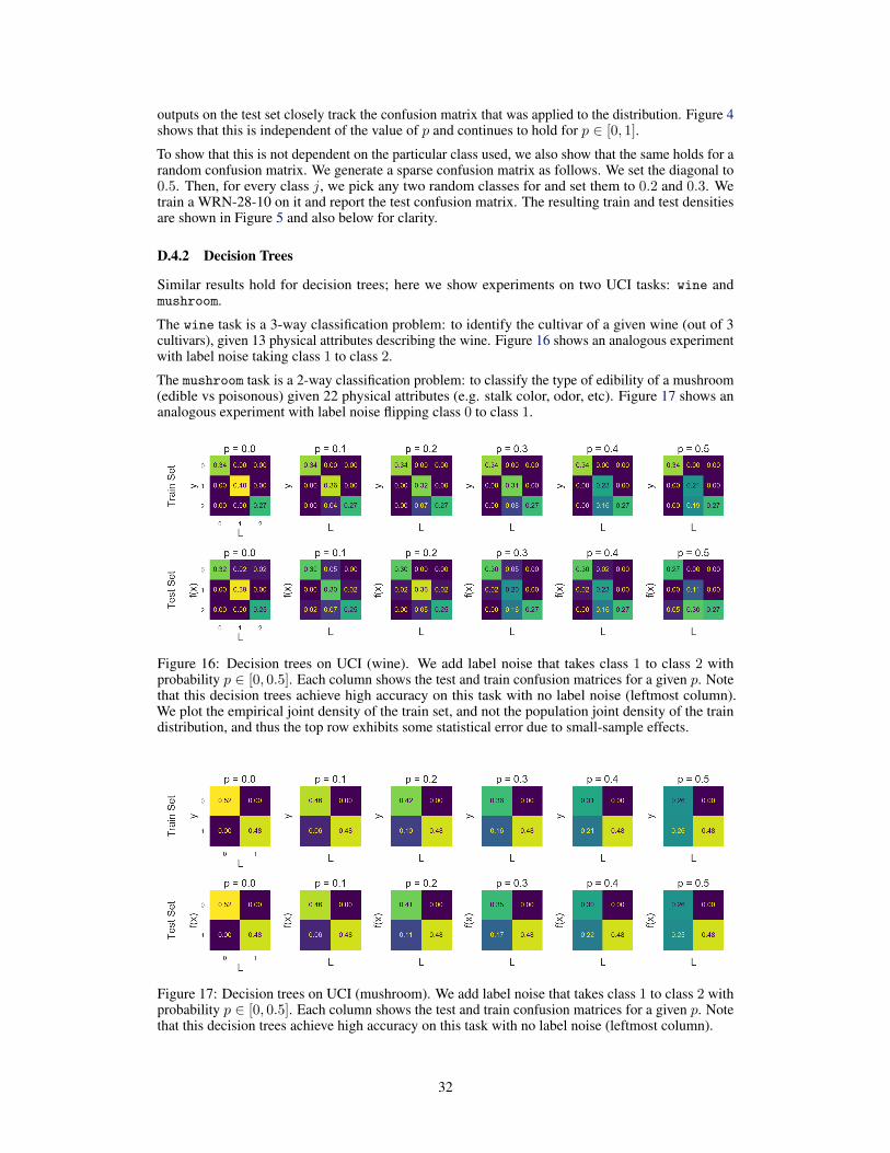
outputs on the test set closely track the confusion matrix that was applied to the distribution. Figure 4shows that this is independent of the value of p and continues to hold for p ∈ [0, 1].

To show that this is not dependent on the particular class used, we also show that the same holds for arandom confusion matrix. We generate a sparse confusion matrix as follows. We set the diagonal to0.5. Then, for every class j, we pick any two random classes for and set them to 0.2 and 0.3. Wetrain a WRN-28-10 on it and report the test confusion matrix. The resulting train and test densitiesare shown in Figure 5 and also below for clarity.

D.4.2 Decision Trees

Similar results hold for decision trees; here we show experiments on two UCI tasks: wine andmushroom.

The wine task is a 3-way classification problem: to identify the cultivar of a given wine (out of 3cultivars), given 13 physical attributes describing the wine. Figure 16 shows an analogous experimentwith label noise taking class 1 to class 2.

The mushroom task is a 2-way classification problem: to classify the type of edibility of a mushroom(edible vs poisonous) given 22 physical attributes (e.g. stalk color, odor, etc). Figure 17 shows ananalogous experiment with label noise flipping class 0 to class 1.

Figure 16: Decision trees on UCI (wine). We add label noise that takes class 1 to class 2 withprobability p ∈ [0, 0.5]. Each column shows the test and train confusion matrices for a given p. Notethat this decision trees achieve high accuracy on this task with no label noise (leftmost column).We plot the empirical joint density of the train set, and not the population joint density of the traindistribution, and thus the top row exhibits some statistical error due to small-sample effects.

Figure 17: Decision trees on UCI (mushroom). We add label noise that takes class 1 to class 2 withprobability p ∈ [0, 0.5]. Each column shows the test and train confusion matrices for a given p. Notethat this decision trees achieve high accuracy on this task with no label noise (leftmost column).

32

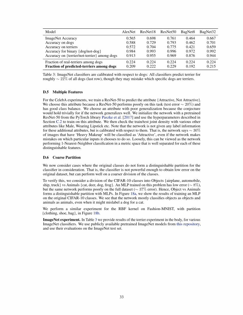
Model AlexNet ResNet18 ResNet50 BagNet8 BagNet32

ImageNet Accuracy 0.565 0.698 0.761 0.464 0.667Accuracy on dogs 0.588 0.729 0.793 0.462 0.701Accuracy on terriers 0.572 0.704 0.775 0.421 0.659Accuracy for binary {dog/not-dog} 0.984 0.993 0.996 0.972 0.992Accuracy on {terrier/not-terrier} among dogs 0.913 0.955 0.969 0.876 0.944

Fraction of real-terriers among dogs 0.224 0.224 0.224 0.224 0.224Fraction of predicted-terriers among dogs 0.209 0.222 0.229 0.192 0.215

Table 3: ImageNet classifiers are calibrated with respect to dogs: All classifiers predict terrier forroughly ∼ 22% of all dogs (last row), though they may mistake which specific dogs are terriers.

D.5 Multiple Features

For the CelebA experiments, we train a ResNet-50 to predict the attribute {Attractive, Not Attractive}.We choose this attribute because a ResNet-50 performs poorly on this task (test error ∼ 20%) andhas good class balance. We choose an attribute with poor generalization because the conjecturewould hold trivially for if the network generalizes well. We initialize the network with a pretrainedResNet-50 from the PyTorch library Paszke et al. [2017] and use the hyperparameters described inSection C.2 to train on this attribute. We then check the train/test joint density with various otherattributes like Male, Wearing Lipstick etc. Note that the network is not given any label informationfor these additional attributes, but is calibrated with respect to them. That is, the network says ∼ 30%of images that have ‘Heavy Makeup’ will be classified as ‘Attractive’, even if the network makesmistakes on which particular inputs it chooses to do so. Loosely, this can be viewed as the networkperforming 1-Nearest-Neighbor classification in a metric space that is well separated for each of thesedistinguishable features.

D.6 Coarse Partition

We now consider cases where the original classes do not form a distinguishable partition for theclassifier in consideration. That is, the classifier is not powerful enough to obtain low error on theoriginal dataset, but can perform well on a coarser division of the classes.

To verify this, we consider a division of the CIFAR-10 classes into Objects {airplane, automobile,ship, truck} vs Animals {cat, deer, dog, frog}. An MLP trained on this problem has low error (∼ 8%),but the same network performs poorly on the full dataset (∼ 37% error). Hence, Object vs Animalsforms a distinguishable partition with MLPs. In Figure 18a, we show the results of training an MLPon the original CIFAR-10 classes. We see that the network mostly classifies objects as objects andanimals as animals, even when it might mislabel a dog for a cat.

We perform a similar experiment for the RBF kernel on Fashion-MNIST, with partition{clothing, shoe, bag}, in Figure 18b.

ImageNet experiment. In Table 3 we provide results of the terrier experiment in the body, for variousImageNet classifiers. We use publicly available pretrained ImageNet models from this repository,and use their evaluations on the ImageNet test set.

33

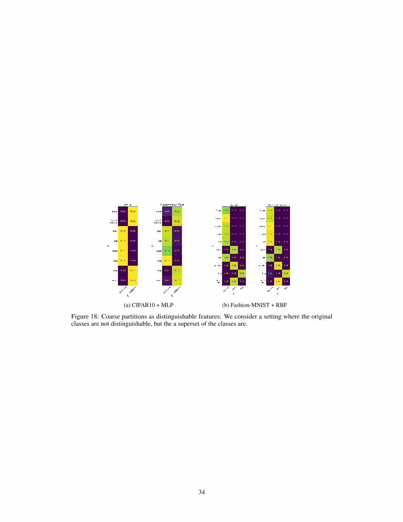
(a) CIFAR10 + MLP (b) Fashion-MNIST + RBF

Figure 18: Coarse partitions as distinguishable features: We consider a setting where the originalclasses are not distinguishable, but the a superset of the classes are.

34

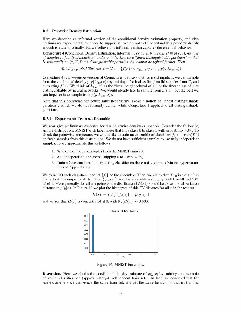
D.7 Pointwise Density Estimation

Here we describe an informal version of the conditional-density estimation property, and givepreliminary experimental evidence to support it. We do not yet understand this property deeplyenough to state it formally, but we believe this informal version captures the essential behavior.Conjecture 4 (Conditional Density Estimation, Informal). For all distributionsD ≡ p(x, y), numberof samples n, family of models F , and ε > 0, let Lfine be a “finest distinguishable partition” — thatis, informally an (ε,F ,D, n)-distinguishable partition that cannot be refined further. Then:

With high probability over x ∼ D : {f(x)}f←TrainF (Dn) ≈ε p(y|Lfine(x))

Conjecture 4 is a pointwise version of Conjecture 1: it says that for most inputs x, we can samplefrom the conditional density p(y|Lfine(x)) by training a fresh classifier f on iid samples from D, andoutputting f(x). We think of Lfine(x) as the “local neighborhood of x”, or the finest class of x asdistinguishable by neural networks. We would ideally like to sample from p(y|x), but the best wecan hope for is to sample from p(y|Lfine(x)).

Note that this pointwise conjecture must neccesarily invoke a notion of “finest distinguishablepartition”, which we do not formally define, while Conjecture 1 applied to all distinguishablepartitions.

D.7.1 Experiment: Train-set Ensemble

We now give preliminary evidence for this pointwise density estimation. Consider the followingsimple distribution: MNIST with label noise that flips class 0 to class 1 with probability 40%. Tocheck the pointwise conjecture, we would like to train an ensemble of classifiers fi ← Train(Dn)on fresh samples from this distribution. We do not have sufficient samples to use truly independentsamples, so we approximate this as follows:

1. Sample 5k random examples from the MNIST-train set.2. Add independent label noise (flipping 0 to 1 w.p. 40%).3. Train a Gaussian kernel interpolating classifier on these noisy samples (via the hyperparam-

eters in Appendix C).

We train 100 such classifiers, and let {fi} be the ensemble. Then, we claim that if x0 is a digit 0 inthe test set, the empirical distribution {fi(x0)} over the ensemble is roughly 60% label-0 and 40%label-1. More generally, for all test points x, the distribution {fi(x)} should be close in total variationdistance to p(y|x). In Figure 19 we plot the histogram of this TV distance for all x in the test set

H(x) := TV ( {fi(x)} , p(y|x) )

and we see that H(x) is concentrated at 0, with Ex[H(x)] ≈ 0.036.

Figure 19: MNIST Ensemble.

Discussion. Here we obtained a conditional density estimate of p(y|x) by training an ensembleof kernel classifiers on (approximately-) independent train sets. In fact, we observed that forsome classifiers we can re-use the same train set, and get the same behavior – that is, training

35

an ensemble with fresh random initialization alone. In these cases, randomness in the trainingprocedure is somehow able to substitute for randomness in the sampling procedure. This cannothold for deterministic training procedures, such as kernel regression, but we have observed it forneural-networks and decision trees. The corresponding statement about decision trees is implicitin works on the conditional-density-estimation properties of random forests (e.g. Olson and Wyner[2018]).

36

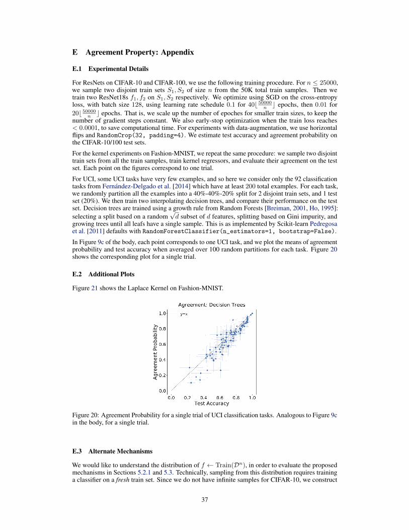
E Agreement Property: Appendix

E.1 Experimental Details

For ResNets on CIFAR-10 and CIFAR-100, we use the following training procedure. For n ≤ 25000,we sample two disjoint train sets S1, S2 of size n from the 50K total train samples. Then wetrain two ResNet18s f1, f2 on S1, S2 respectively. We optimize using SGD on the cross-entropyloss, with batch size 128, using learning rate schedule 0.1 for 40b 50000n c epochs, then 0.01 for20b 50000n c epochs. That is, we scale up the number of epoches for smaller train sizes, to keep thenumber of gradient steps constant. We also early-stop optimization when the train loss reaches< 0.0001, to save computational time. For experiments with data-augmentation, we use horizontalflips and RandomCrop(32, padding=4). We estimate test accuracy and agreement probability onthe CIFAR-10/100 test sets.

For the kernel experiments on Fashion-MNIST, we repeat the same procedure: we sample two disjointtrain sets from all the train samples, train kernel regressors, and evaluate their agreement on the testset. Each point on the figures correspond to one trial.

For UCI, some UCI tasks have very few examples, and so here we consider only the 92 classificationtasks from Fernández-Delgado et al. [2014] which have at least 200 total examples. For each task,we randomly partition all the examples into a 40%-40%-20% split for 2 disjoint train sets, and 1 testset (20%). We then train two interpolating decision trees, and compare their performance on the testset. Decision trees are trained using a growth rule from Random Forests [Breiman, 2001, Ho, 1995]:selecting a split based on a random

√d subset of d features, splitting based on Gini impurity, and

growing trees until all leafs have a single sample. This is as implemented by Scikit-learn Pedregosaet al. [2011] defaults with RandomForestClassifier(n_estimators=1, bootstrap=False).

In Figure 9c of the body, each point corresponds to one UCI task, and we plot the means of agreementprobability and test accuracy when averaged over 100 random partitions for each task. Figure 20shows the corresponding plot for a single trial.

E.2 Additional Plots

Figure 21 shows the Laplace Kernel on Fashion-MNIST.

Figure 20: Agreement Probability for a single trial of UCI classification tasks. Analogous to Figure 9cin the body, for a single trial.

E.3 Alternate Mechanisms

We would like to understand the distribution of f ← Train(Dn), in order to evaluate the proposedmechanisms in Sections 5.2.1 and 5.3. Technically, sampling from this distribution requires traininga classifier on a fresh train set. Since we do not have infinite samples for CIFAR-10, we construct

37

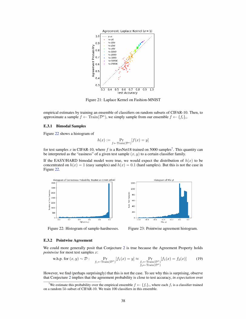
Figure 21: Laplace Kernel on Fashion-MNIST

empirical estimates by training an ensemble of classifiers on random subsets of CIFAR-10. Then, toapproximate a sample f ← Train(Dn), we simply sample from our ensemble f ← {fi}i.

E.3.1 Bimodal Samples

Figure 22 shows a histogram of

h(x) := Prf←Train(Dn)

[f(x) = y]

for test samples x in CIFAR-10, where f is a ResNet18 trained on 5000 samples7. This quantity canbe interpreted as the “easiness” of a given test sample (x, y) to a certain classifier family.

If the EASY/HARD bimodal model were true, we would expect the distribution of h(x) to beconcentrated on h(x) = 1 (easy samples) and h(x) = 0.1 (hard samples). But this is not the case inFigure 22.

Figure 22: Histogram of sample-hardnesses. Figure 23: Pointwise agreement histogram.

E.3.2 Pointwise Agreement

We could more generally posit that Conjecture 2 is true because the Agreement Property holdspointwise for most test samples x:

w.h.p. for (x, y) ∼ D : Prf1←Train(Dn)

[f1(x) = y] ≈ Prf1←Train(Dn)f2←Train(Dn)

[f1(x) = f2(x)] (19)

However, we find (perhaps surprisingly) that this is not the case. To see why this is surprising, observethat Conjecture 2 implies that the agreement probability is close to test accuracy, in expectation over

7We estimate this probability over the empirical ensemble f ← {fi}i, where each fi is a classifier trainedon a random 5k-subset of CIFAR-10. We train 100 classifiers in this ensemble.

38

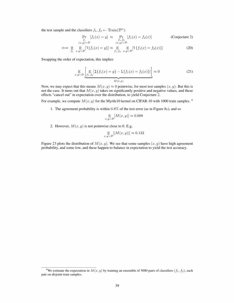
the test sample and the classifiers f1, f2 ← Train(Dn):

Prf1

(x,y)∼D

[f1(x) = y] ≈ Prf1,f2

(x,y)∼D

[f1(x) = f2(x)] (Conjecture 2)

⇐⇒ Ef1

Ex,y∼D

[1{f1(x) = y}] ≈ Ef1,f2

Ex,y∼D

[1{f1(x) = f2(x)}] (20)

Swapping the order of expectation, this implies

Ex,y∼D

[E

f1,f2[1{f1(x) = y} − 1{f1(x) = f2(x)}]

]︸ ︷︷ ︸

M(x,y)

≈ 0 (21)

Now, we may expect that this means M(x, y) ≈ 0 pointwise, for most test samples (x, y). But this isnot the case. It turns out that M(x, y) takes on significantly positive and negative values, and theseeffects “cancel out” in expectation over the distribution, to yield Conjecture 2.

For example, we compute M(x, y) for the Myrtle10 kernel on CIFAR-10 with 1000 train samples. 8

1. The agreement probability is within 0.8% of the test error (as in Figure 8c), and so

Ex,y∼D

[M(x, y)] ≈ 0.008

2. However, M(x, y) is not pointwise close to 0. E.g,

Ex,y∼D

[|M(x, y)|] ≈ 0.133

Figure 23 plots the distribution of M(x, y). We see that some samples (x, y) have high agreementprobability, and some low, and these happen to balance in expectation to yield the test accuracy.

8We estimate the expectation in M(x, y) by training an ensemble of 5000 pairs of classifiers (f1, f2), eachpair on disjoint train samples.

39

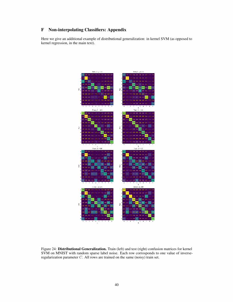
F Non-interpolating Classifiers: Appendix

Here we give an additional example of distributional generalization: in kernel SVM (as opposed tokernel regression, in the main text).

Figure 24: Distributional Generalization. Train (left) and test (right) confusion matrices for kernelSVM on MNIST with random sparse label noise. Each row corrosponds to one value of inverse-regularization parameter C. All rows are trained on the same (noisy) train set.

40

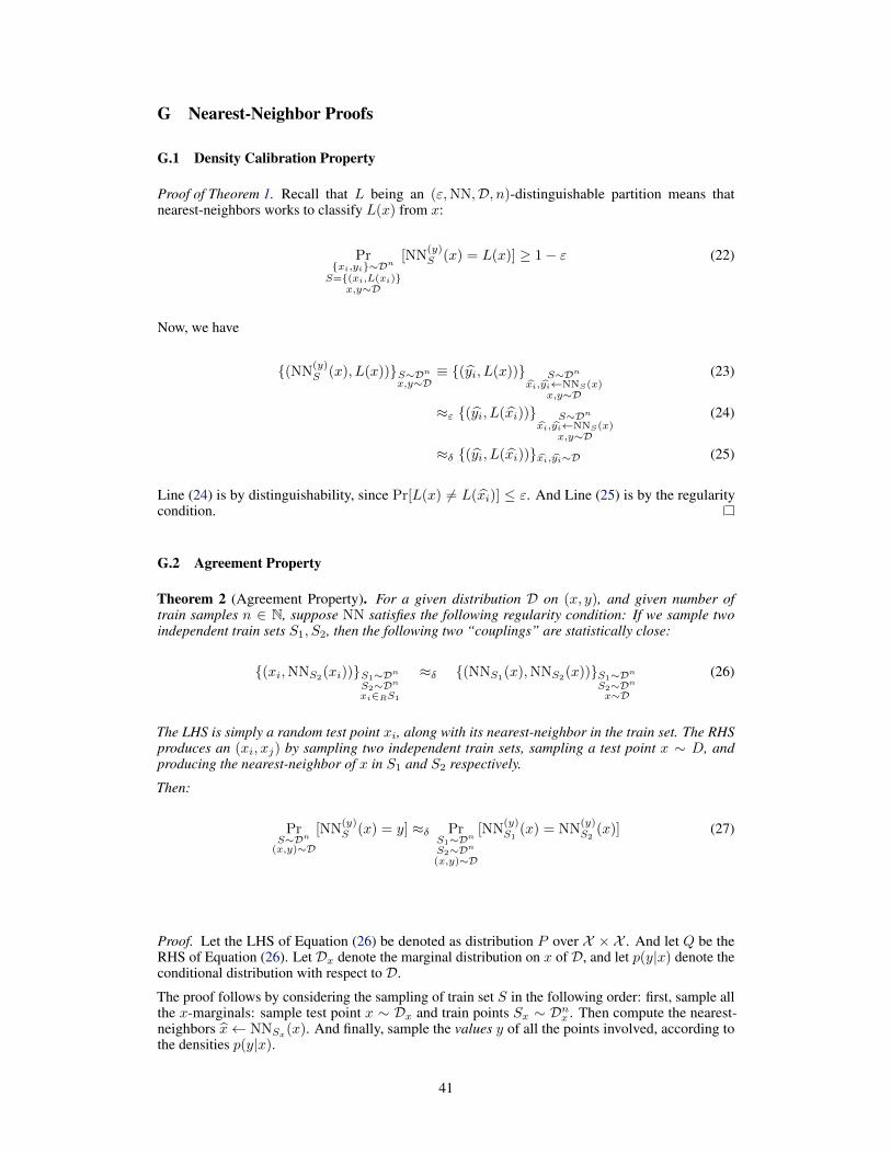
G Nearest-Neighbor Proofs

G.1 Density Calibration Property

Proof of Theorem 1. Recall that L being an (ε,NN,D, n)-distinguishable partition means thatnearest-neighbors works to classify L(x) from x:

Pr{xi,yi}∼Dn

S={(xi,L(xi)}x,y∼D

[NN(y)S (x) = L(x)] ≥ 1− ε (22)

Now, we have

{(NN(y)S (x), L(x))}S∼Dn

x,y∼D≡ {(yi, L(x))} S∼Dn

xi,yi←NNS(x)x,y∼D

(23)

≈ε {(yi, L(xi))} S∼Dn

xi,yi←NNS(x)x,y∼D

(24)

≈δ {(yi, L(xi))}xi,yi∼D (25)

Line (24) is by distinguishability, since Pr[L(x) 6= L(xi)] ≤ ε. And Line (25) is by the regularitycondition.

G.2 Agreement Property

Theorem 2 (Agreement Property). For a given distribution D on (x, y), and given number oftrain samples n ∈ N, suppose NN satisfies the following regularity condition: If we sample twoindependent train sets S1, S2, then the following two “couplings” are statistically close:

{(xi,NNS2(xi))}S1∼Dn

S2∼Dn

xi∈RS1

≈δ {(NNS1(x),NNS2

(x))}S1∼Dn

S2∼Dn

x∼D

(26)

The LHS is simply a random test point xi, along with its nearest-neighbor in the train set. The RHSproduces an (xi, xj) by sampling two independent train sets, sampling a test point x ∼ D, andproducing the nearest-neighbor of x in S1 and S2 respectively.

Then:

PrS∼Dn

(x,y)∼D

[NN(y)S (x) = y] ≈δ Pr

S1∼Dn

S2∼Dn

(x,y)∼D

[NN(y)S1

(x) = NN(y)S2

(x)] (27)

Proof. Let the LHS of Equation (26) be denoted as distribution P over X × X . And let Q be theRHS of Equation (26). Let Dx denote the marginal distribution on x of D, and let p(y|x) denote theconditional distribution with respect to D.

The proof follows by considering the sampling of train set S in the following order: first, sample allthe x-marginals: sample test point x ∼ Dx and train points Sx ∼ Dnx . Then compute the nearest-neighbors x← NNSx

(x). And finally, sample the values y of all the points involved, according tothe densities p(y|x).

41

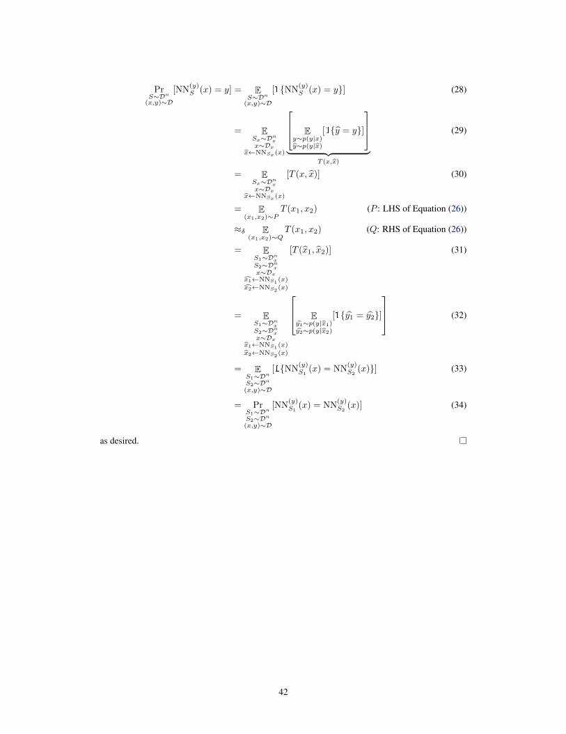
PrS∼Dn

(x,y)∼D

[NN(y)S (x) = y] = E

S∼Dn

(x,y)∼D

[1{NN(y)S (x) = y}] (28)

= ESx∼Dn

xx∼Dx

x←NNSx (x)

Ey∼p(y|x)y∼p(y|x)

[1{y = y}]

︸ ︷︷ ︸

T (x,x)

(29)

= ESx∼Dn

xx∼Dx

x←NNSx (x)

[T (x, x)] (30)

= E(x1,x2)∼P

T (x1, x2) (P : LHS of Equation (26))

≈δ E(x1,x2)∼Q

T (x1, x2) (Q: RHS of Equation (26))

= ES1∼Dn

xS2∼Dn

xx∼Dx

x1←NNS1(x)

x2←NNS2(x)

[T (x1, x2)] (31)

= ES1∼Dn

xS2∼Dn

xx∼Dx

x1←NNS1(x)

x2←NNS2(x)

Ey1∼p(y|x1)y2∼p(y|x2)

[1{y1 = y2}]

(32)

= ES1∼Dn

S2∼Dn

(x,y)∼D

[1{NN(y)S1

(x) = NN(y)S2

(x)}] (33)

= PrS1∼Dn

S2∼Dn

(x,y)∼D

[NN(y)S1

(x) = NN(y)S2

(x)] (34)

as desired.

42