Embed Size (px)
Citation preview

SCALABLE AND ROBUST DATA CLUSTERING AND
VISUALIZATION
Yang RuanPhD Candidate
Computer Science DepartmentIndiana University
Outline
• Overview• Research Issues• Experimental Analysis• Conclusion and Futurework
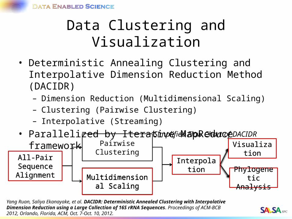
Data Clustering and Visualization• Deterministic Annealing Clustering and Interpolative
Dimension Reduction Method (DACIDR)– Dimension Reduction (Multidimensional Scaling)– Clustering (Pairwise Clustering)– Interpolative (Streaming)
• Parallelized by Iterative MapReduce framework
All-Pair Sequence Alignment
Interpolation
Pairwise Clustering
Multidimensional Scaling
Visualization
Simplified Flow Chart of DACIDR
Phylogenetic Analysis
All-Pair Sequence Alignment
Interpolation
Multidimensional Scaling
Visualization
Phylogenetic Analysis
Yang Ruan, Saliya Ekanayake, et al. DACIDR: Deterministic Annealed Clustering with Interpolative Dimension Reduction using a Large Collection of 16S rRNA Sequences. Proceedings of ACM-BCB 2012, Orlando, Florida, ACM, Oct. 7-Oct. 10, 2012.
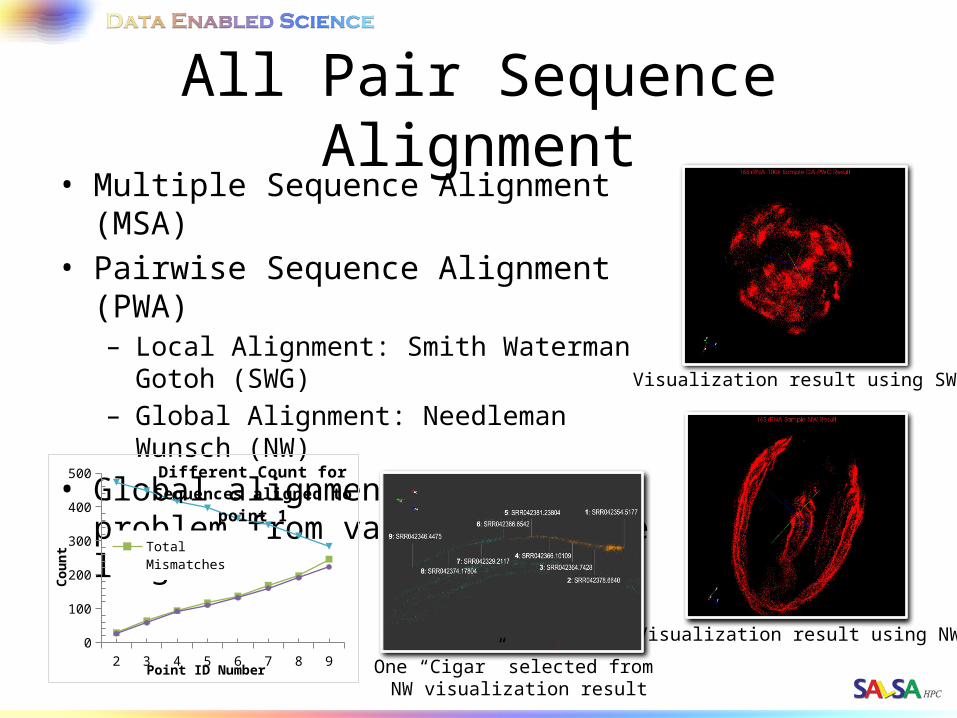
All Pair Sequence Alignment• Multiple Sequence Alignment (MSA)• Pairwise Sequence Alignment (PWA)
– Local Alignment: Smith Waterman Gotoh (SWG)
– Global Alignment: Needleman Wunsch (NW)
• Global alignment suffers problem from various sequence lengths
Visualization result using SWG
Visualization result using NW2 3 4 5 6 7 8 9
0
100
200
300
400
500 Different Count for Sequences aligned to point 1
Total MismatchesMismatches by GapsOriginal Length
Point ID Number
Coun
t
One “Cigar” selected from NW visualization result
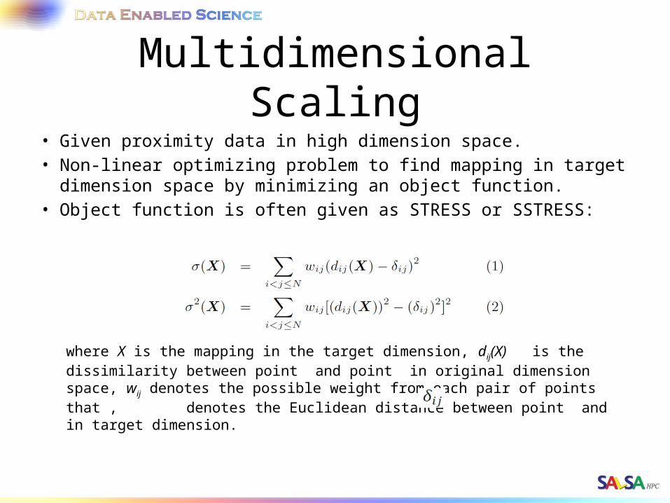
Multidimensional Scaling• Given proximity data in high dimension space.• Non-linear optimizing problem to find mapping in target
dimension space by minimizing an object function.• Object function is often given as STRESS or SSTRESS:
where X is the mapping in the target dimension, dij(X) is the dissimilarity between point and point in original dimension space, wij denotes the possible weight from each pair of points that , denotes the Euclidean distance between point and in target dimension.
Interpolation• Out-of-sample / Streaming / Interpolation problem
– Original MDS algorithm needs O(N2) memory.– Given an in-sample data result, interpolate out-of-sample into the
in-sample target dimension space.
• Reduce space complexity and time complexity of MDS– Select part of data as in-sample dataset, apply MDS on that– Remaining data are out-of-sample dataset, and interpolated into the
target dimension space using the result from in-sample space.– Computation complexity is reduced to linear.– Space complexity is reduced to constant.
Possible Issues• Local sequence alignment (SWG) could generate very low
quality distances.– E.g. For two sequences with original length 500, it could generate
an alignment with length 10 and gives a pid of 1 (distance 0) even if these two sequences shouldn’t be near each other.
• Sequence alignment is time consuming.– E.g. To interpolate 100k out-of-sample sequences (average length of
500) into 10k in-sample sequences took around 100 seconds to finish on 400 cores, but to align them took around 6000 seconds to finish on same number of cores.
• Phylogenetic Analysis separates from clustering– Current phylogenetic tree displaying methods does NOT allow the
display of tree seamlessly with clusters.
Contribution• MDS algorithm generalization with weight (WDA-SMACOF)
– Reduced time complexity to quadratic– Solves problems with fixed part of points
• Time Cost Reduction of Interpolation with Weighting– W-MI-MDS that generalize interpolations with weighting– Hierarchical MI-MDS that reduces the time cost
• Enable seamless observation of Phylogenetic tree and clustering together.– Cuboid Cladogram– Spherical Phylogram
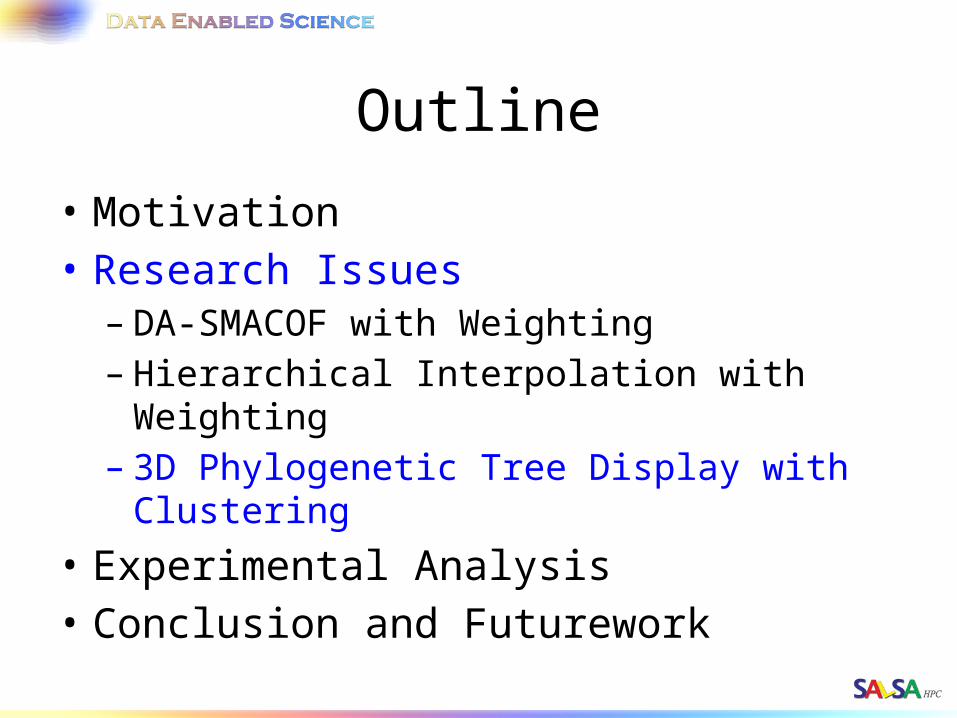
Outline
• Motivation• Research Issues– DA-SMACOF with Weighting– Hierarchical Interpolation with Weighting– 3D Phylogenetic Tree Display with Clustering
• Experimental Analysis• Conclusion and Futurework
WDA-SMACOF (background)
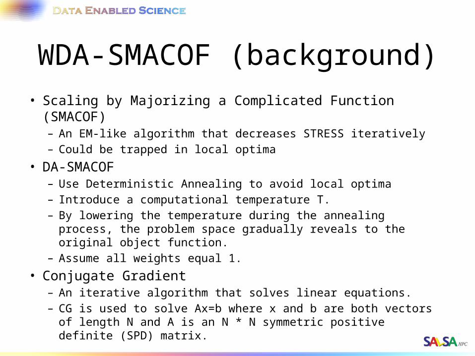
• Scaling by Majorizing a Complicated Function (SMACOF)– An EM-like algorithm that decreases STRESS iteratively– Could be trapped in local optima
• DA-SMACOF– Use Deterministic Annealing to avoid local optima– Introduce a computational temperature T.– By lowering the temperature during the annealing process, the
problem space gradually reveals to the original object function. – Assume all weights equal 1.
• Conjugate Gradient– An iterative algorithm that solves linear equations.– CG is used to solve Ax=b where x and b are both vectors of length
N and A is an N * N symmetric positive definite (SPD) matrix.
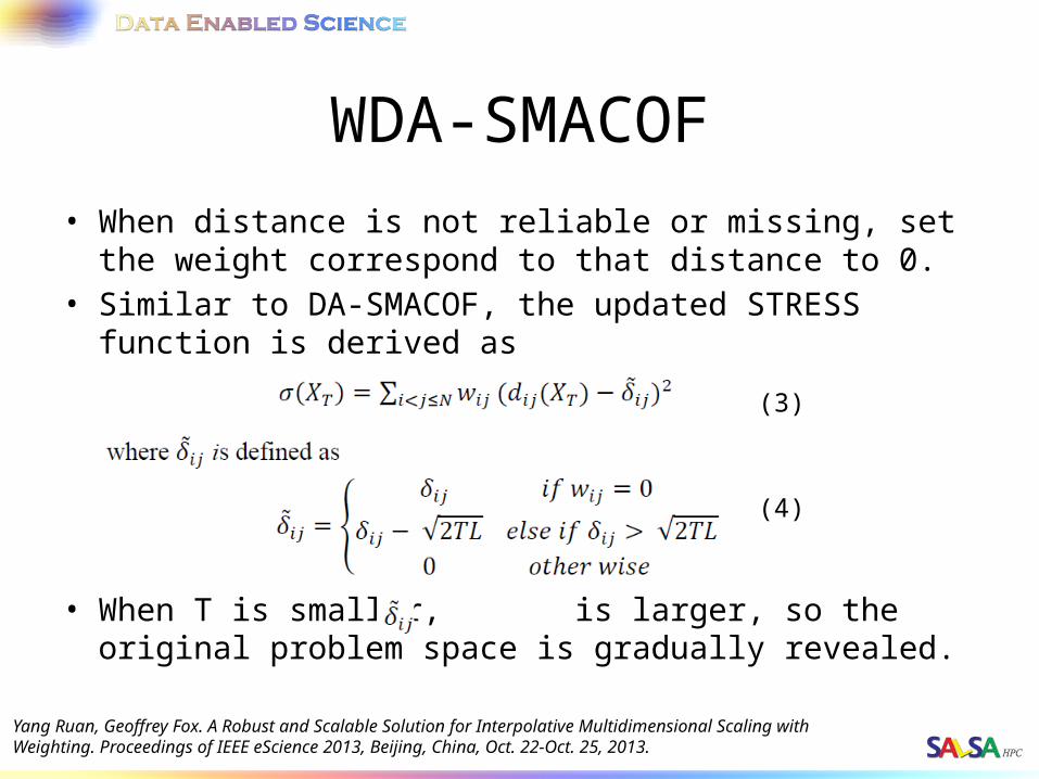
WDA-SMACOF• When distance is not reliable or missing, set the weight
correspond to that distance to 0.• Similar to DA-SMACOF, the updated STRESS function is
derived as
• When T is smaller, is larger, so the original problem space is gradually revealed.
(3)
(4)
Yang Ruan, Geoffrey Fox. A Robust and Scalable Solution for Interpolative Multidimensional Scaling with Weighting. Proceedings of IEEE eScience 2013, Beijing, China, Oct. 22-Oct. 25, 2013.
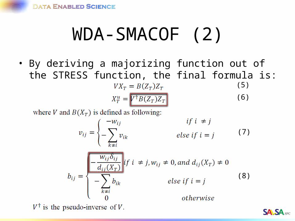
WDA-SMACOF (2)• By deriving a majorizing function out of the STRESS
function, the final formula is:
(6)
(5)
(7)
(8)
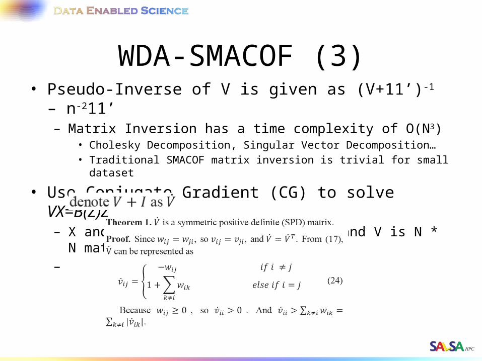
WDA-SMACOF (3)• Pseudo-Inverse of V is given as (V+11’)-1 – n-211’
– Matrix Inversion has a time complexity of O(N3)• Cholesky Decomposition, Singular Vector Decomposition…• Traditional SMACOF matrix inversion is trivial for small dataset
• Use Conjugate Gradient (CG) to solve VX=B(Z)Z– X and B(Z)Z are both N * L matrix and V is N * N matrix.–
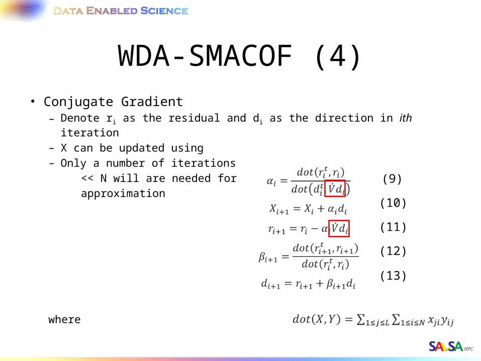
WDA-SMACOF (4)• Conjugate Gradient
– Denote ri as the residual and di as the direction in ith iteration
– X can be updated using– Only a number of iterations << N will are needed for approximation
where
(9)
(10)
(11)
(12)
(13)
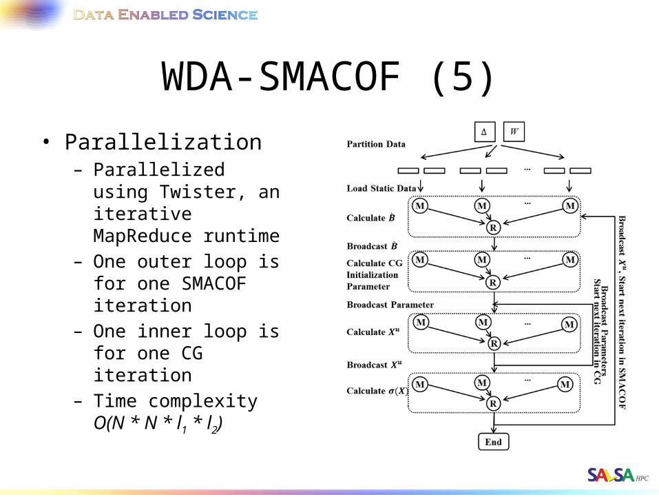
WDA-SMACOF (5)• Parallelization
– Parallelized using Twister, an iterative MapReduce runtime
– One outer loop is for one SMACOF iteration
– One inner loop is for one CG iteration
– Time complexity O(N * N * l1 * l2)
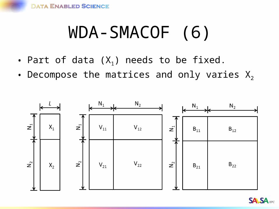
WDA-SMACOF (6)• Part of data (X1) needs to be fixed.
• Decompose the matrices and only varies X2
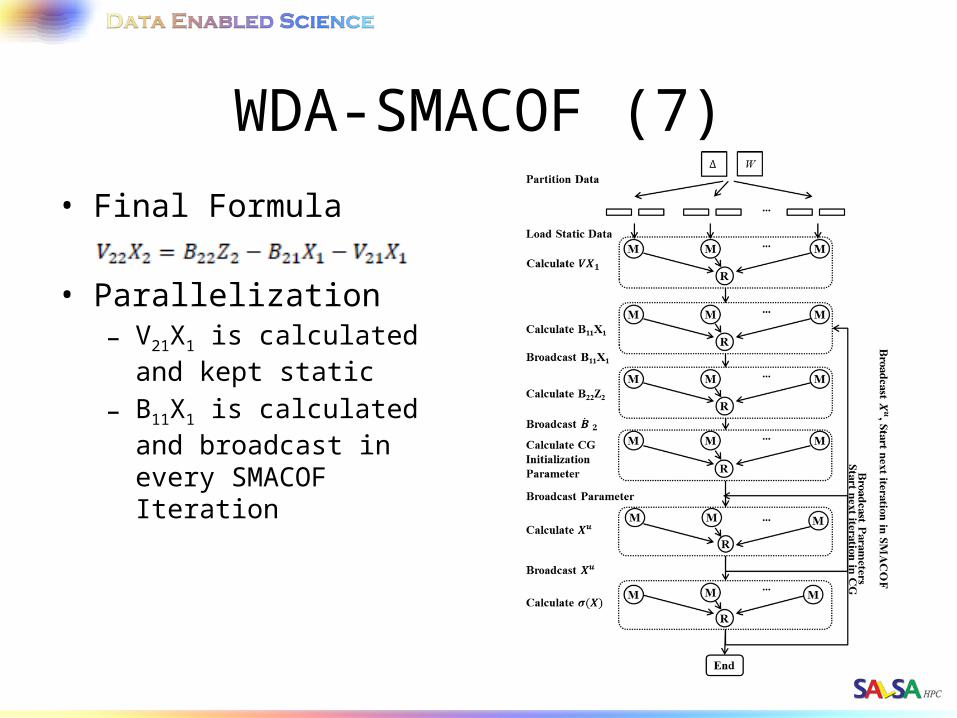
WDA-SMACOF (7)• Final Formula
• Parallelization– V21X1 is calculated and
kept static– B11X1 is calculated and
broadcast in every SMACOF Iteration
Outline
• Motivation• Research Issues– DA-SMACOF with Weighting– Hierarchical Interpolation with Weighting– 3D Phylogenetic Tree Display with Clustering
• Experimental Analysis• Conclusion and Futurework
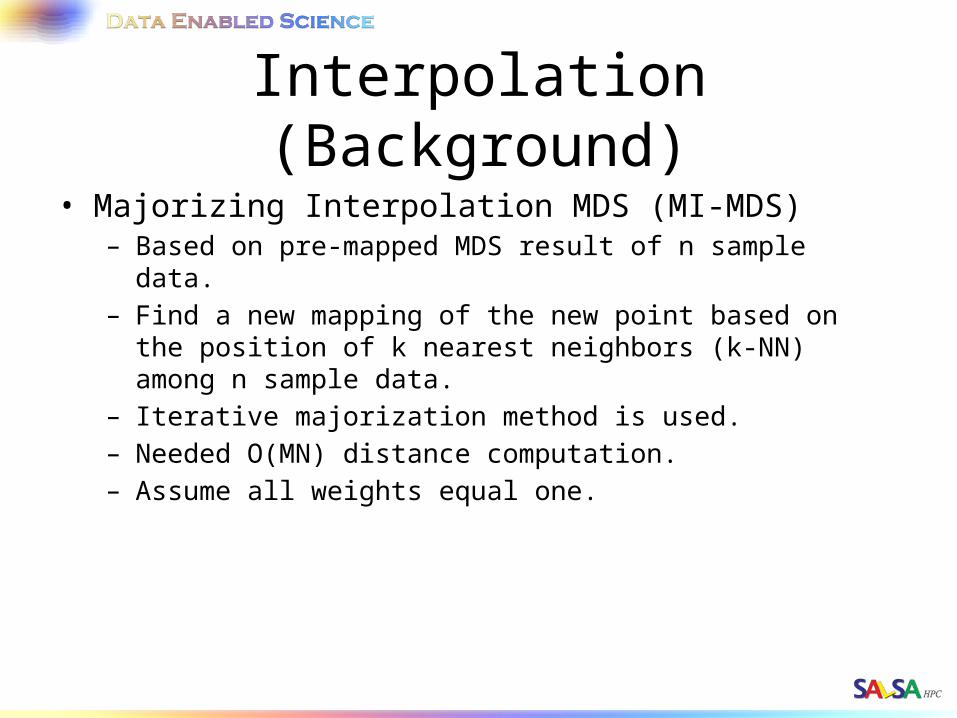
Interpolation (Background)• Majorizing Interpolation MDS (MI-MDS)
– Based on pre-mapped MDS result of n sample data.– Find a new mapping of the new point based on the position of k
nearest neighbors (k-NN) among n sample data.– Iterative majorization method is used.– Needed O(MN) distance computation.– Assume all weights equal one.
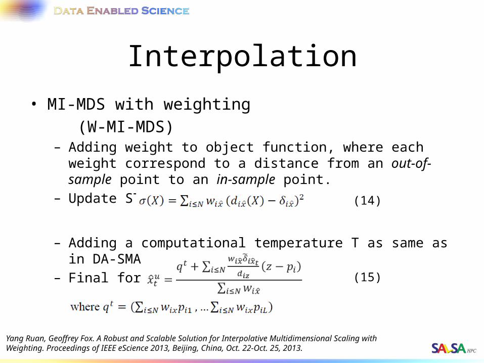
Interpolation• MI-MDS with weighting (W-MI-MDS)
– Adding weight to object function, where each weight correspond to a distance from an out-of-sample point to an in-sample point.
– Update STRESS function:
– Adding a computational temperature T as same as in DA-SMACOF– Final formula is updated as
(14)
(15)
Yang Ruan, Geoffrey Fox. A Robust and Scalable Solution for Interpolative Multidimensional Scaling with Weighting. Proceedings of IEEE eScience 2013, Beijing, China, Oct. 22-Oct. 25, 2013.
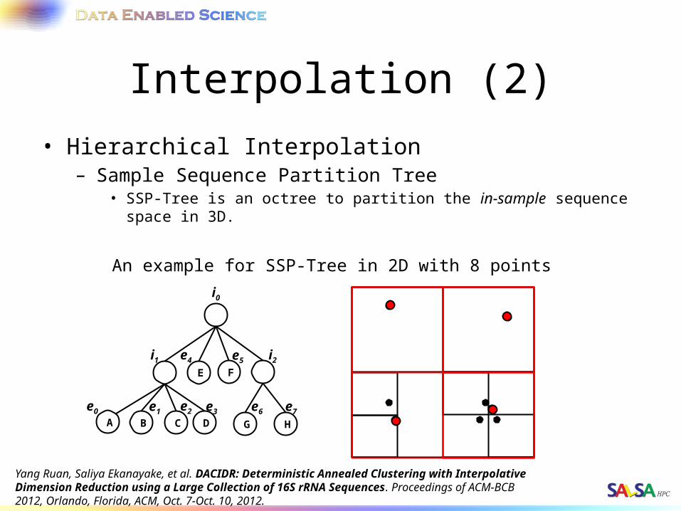
Interpolation (2)• Hierarchical Interpolation
– Sample Sequence Partition Tree• SSP-Tree is an octree to partition the in-sample sequence space in 3D.
a
E F
B CA D G H
e0 e1 e2
e4 e5
e3 e6 e7
i0
i1 i2
An example for SSP-Tree in 2D with 8 points
Yang Ruan, Saliya Ekanayake, et al. DACIDR: Deterministic Annealed Clustering with Interpolative Dimension Reduction using a Large Collection of 16S rRNA Sequences. Proceedings of ACM-BCB 2012, Orlando, Florida, ACM, Oct. 7-Oct. 10, 2012.
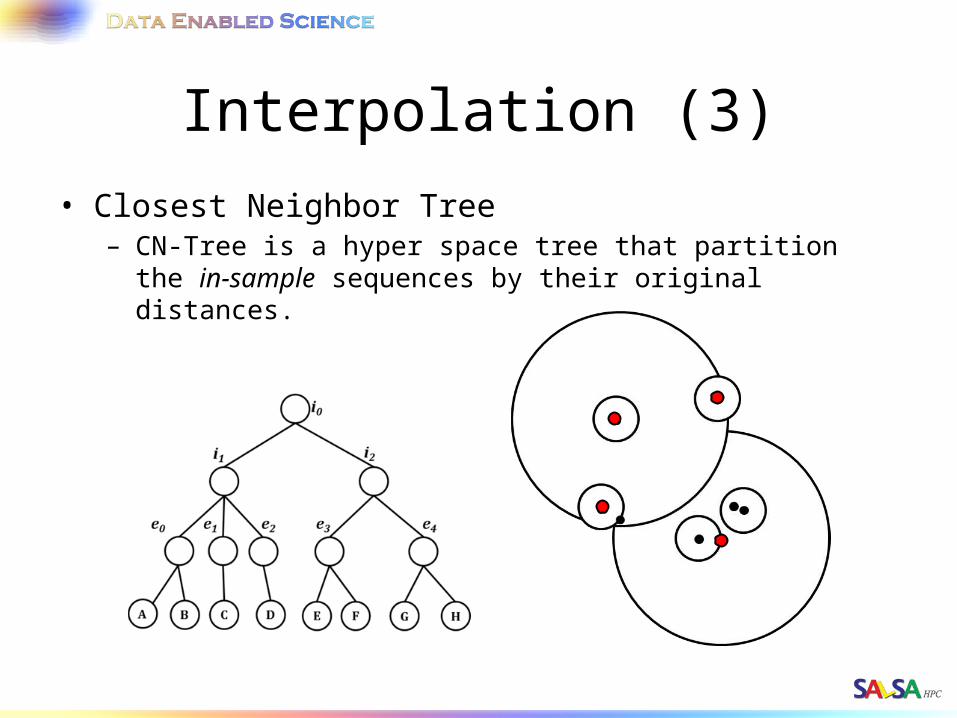
Interpolation (3)• Closest Neighbor Tree
– CN-Tree is a hyper space tree that partition the in-sample sequences by their original distances.
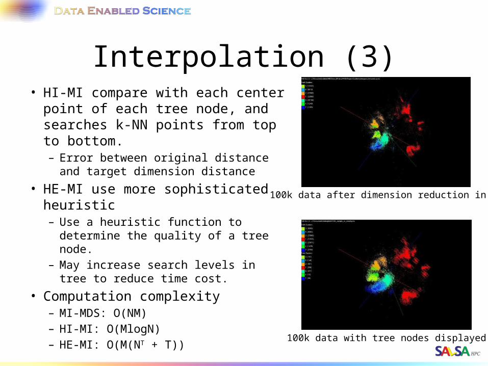
Interpolation (3)• HI-MI compare with each center
point of each tree node, and searches k-NN points from top to bottom.– Error between original distance and
target dimension distance
• HE-MI use more sophisticated heuristic– Use a heuristic function to determine
the quality of a tree node.– May increase search levels in tree to
reduce time cost.
• Computation complexity– MI-MDS: O(NM)– HI-MI: O(MlogN)– HE-MI: O(M(NT + T))
100k data after dimension reduction in 3D
100k data with tree nodes displayed
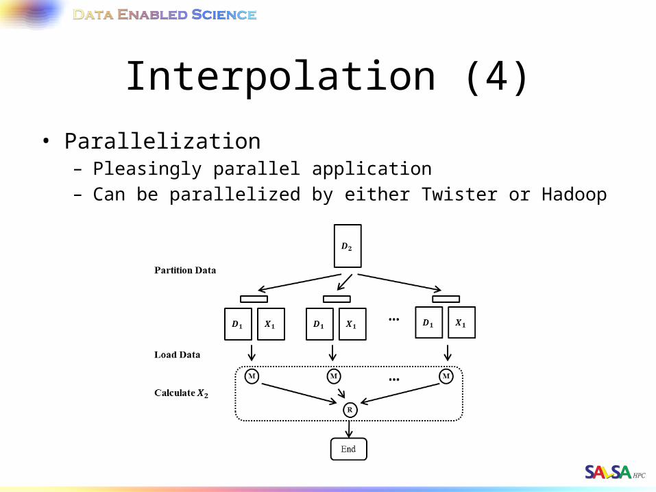
Interpolation (4)• Parallelization
– Pleasingly parallel application– Can be parallelized by either Twister or Hadoop
Outline
• Motivation• Research Issues– DA-SMACOF with Weighting– Hierarchical Interpolation with Weighting– 3D Phylogenetic Tree Display with Clustering
• Experimental Analysis• Conclusion and Futurework
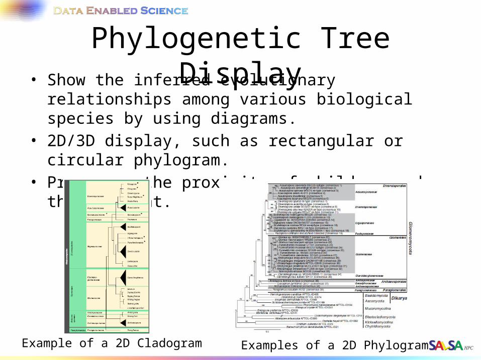
Phylogenetic Tree Display• Show the inferred evolutionary relationships among
various biological species by using diagrams.• 2D/3D display, such as rectangular or circular phylogram.• Preserves the proximity of children and their parent.
Example of a 2D Cladogram Examples of a 2D Phylogram
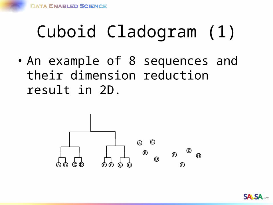
Cuboid Cladogram (1)
• An example of 8 sequences and their dimension reduction result in 2D.
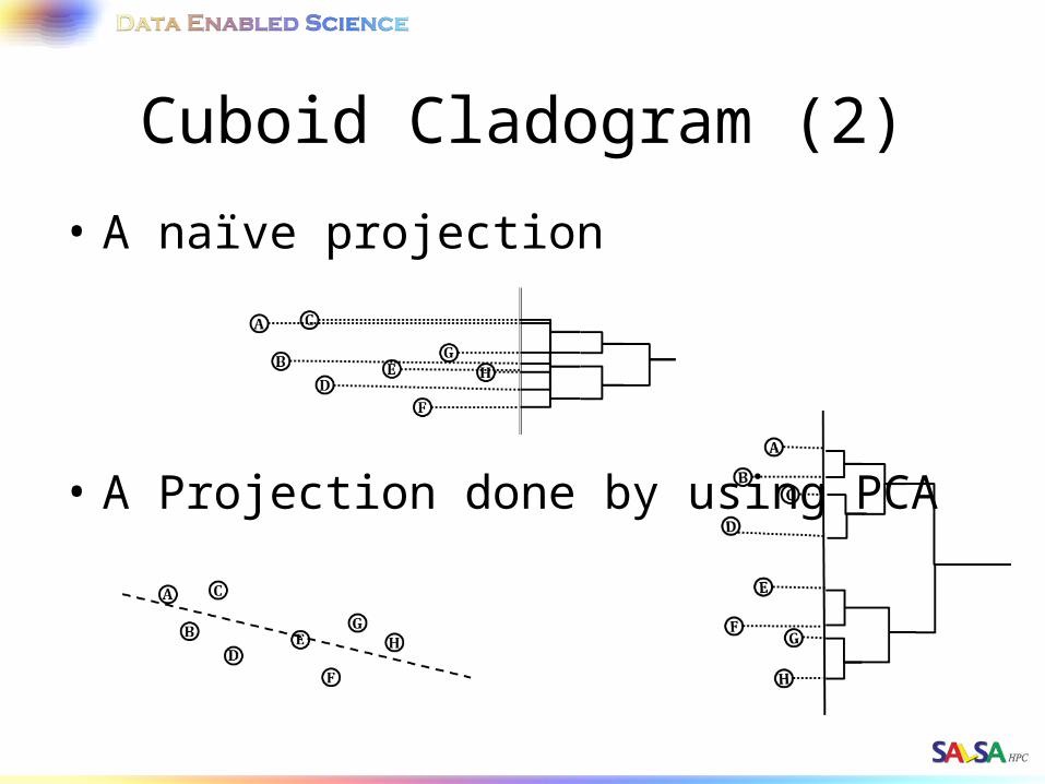
Cuboid Cladogram (2)
• A naïve projection
• A Projection done by using PCA
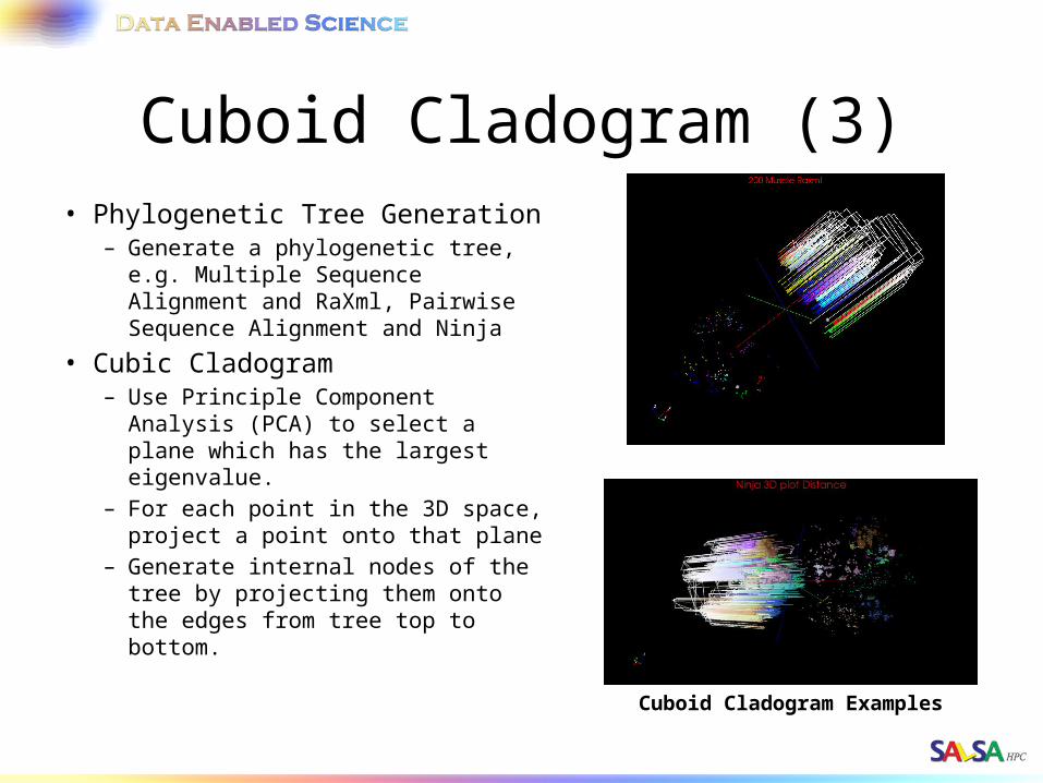
Cuboid Cladogram (3)• Phylogenetic Tree Generation
– Generate a phylogenetic tree, e.g. Multiple Sequence Alignment and RaXml, Pairwise Sequence Alignment and Ninja
• Cubic Cladogram– Use Principle Component
Analysis (PCA) to select a plane which has the largest eigenvalue.
– For each point in the 3D space, project a point onto that plane
– Generate internal nodes of the tree by projecting them onto the edges from tree top to bottom. Cuboid Cladogram Examples
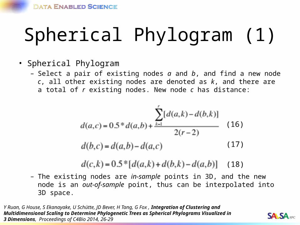
Spherical Phylogram (1)• Spherical Phylogram
– Select a pair of existing nodes a and b, and find a new node c, all other existing nodes are denoted as k, and there are a total of r existing nodes. New node c has distance:
– The existing nodes are in-sample points in 3D, and the new node is an out-of-sample point, thus can be interpolated into 3D space.
(16)
(17)
(18)
Y Ruan, G House, S Ekanayake, U Schütte, JD Bever, H Tang, G Fox , Integration of Clustering and Multidimensional Scaling to Determine Phylogenetic Trees as Spherical Phylograms Visualized in 3 Dimensions, Proceedings of C4Bio 2014, 26-29
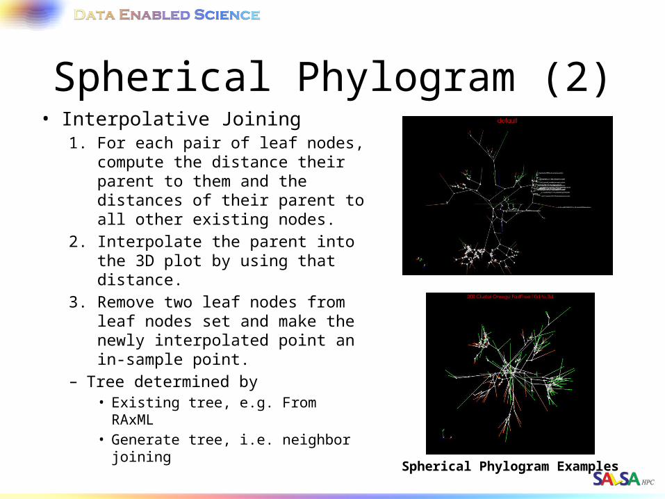
Spherical Phylogram (2)• Interpolative Joining
1. For each pair of leaf nodes, compute the distance their parent to them and the distances of their parent to all other existing nodes.
2. Interpolate the parent into the 3D plot by using that distance.
3. Remove two leaf nodes from leaf nodes set and make the newly interpolated point an in-sample point.
– Tree determined by• Existing tree, e.g. From RAxML• Generate tree, i.e. neighbor
joining Spherical Phylogram Examples
Outline
• Motivation• Background and Related Work• Research Issues• Experimental Analysis– WDA-SMACOF and WDA-MI-MDS– Hierarchical Interpolation– 3D Phylogenetic Tree Display
• Conclusion and Futurework
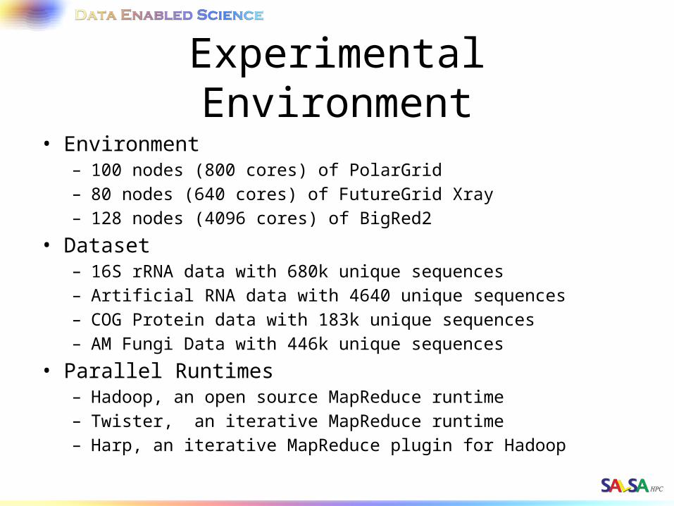
Experimental Environment• Environment
– 100 nodes (800 cores) of PolarGrid– 80 nodes (640 cores) of FutureGrid Xray– 128 nodes (4096 cores) of BigRed2
• Dataset– 16S rRNA data with 680k unique sequences– Artificial RNA data with 4640 unique sequences– COG Protein data with 183k unique sequences– AM Fungi Data with 446k unique sequences
• Parallel Runtimes– Hadoop, an open source MapReduce runtime– Twister, an iterative MapReduce runtime– Harp, an iterative MapReduce plugin for Hadoop
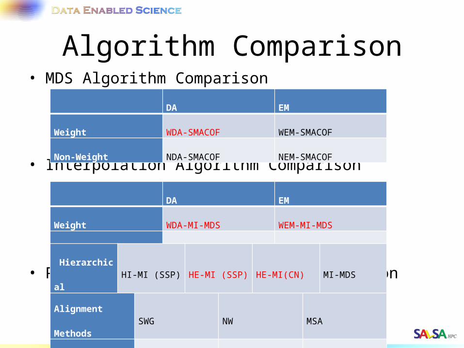
Algorithm Comparison• MDS Algorithm Comparison
• Interpolation Algorithm Comparison
• Phylogenetic Tree Algorithm Comparison
DA EM
Weight WDA-SMACOF WEM-SMACOF
Non-Weight NDA-SMACOF NEM-SMACOF
DA EM
Weight WDA-MI-MDS WEM-MI-MDS
Non-Weight NDA-MI-MDS NEM-MI-MDS
Alignment Methods SWG NW MSA
MDS Methods WDA-SMACOF EM-SMACOF EM-SMACOF
Hierarchical HI-MI (SSP) HE-MI (SSP) HE-MI(CN) MI-MDS
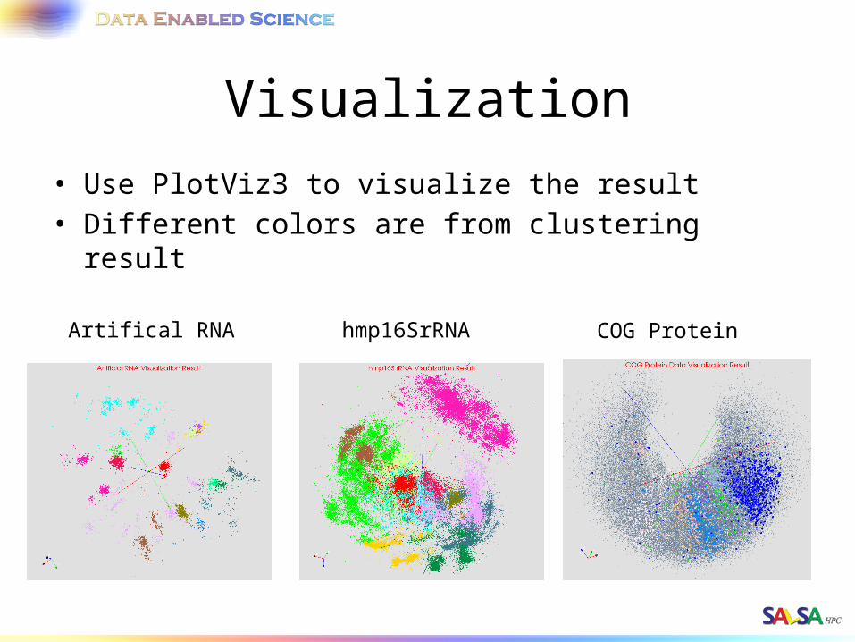
Visualization• Use PlotViz3 to visualize the result• Different colors are from clustering result
Artifical RNA hmp16SrRNA COG Protein
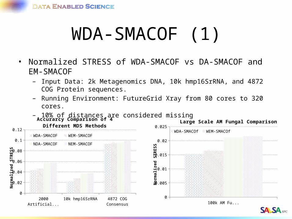
WDA-SMACOF (1)• Normalized STRESS of WDA-SMACOF vs DA-SMACOF and EM-SMACOF
– Input Data: 2k Metagenomics DNA, 10k hmp16SrRNA, and 4872 COG Protein sequences.
– Running Environment: FutureGrid Xray from 80 cores to 320 cores.– 10% of distances are considered missing
100k AM Fungal0
0.005
0.01
0.015
0.02
0.025Large Scale AM Fungal Comparison
WDA-SMACOf WEM-SMACOfNDA-SMACOF NEM-SMACOF
Nor
mal
ized
ST
RE
SS
2000 Artificial RNA 10k hmp16SrRNA 4872 COG Consensus0
0.02
0.04
0.06
0.08
0.1
0.12
Accurarcy Comparison of 4 Different MDS Methods
WDA-SMACOF WEM-SMACOF
NDA-SMACOF NEM-SMACOF
Nor
mal
ized
ST
RE
SS
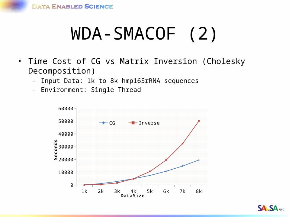
WDA-SMACOF (2)• Time Cost of CG vs Matrix Inversion (Cholesky Decomposition)
– Input Data: 1k to 8k hmp16SrRNA sequences– Environment: Single Thread
1k 2k 3k 4k 5k 6k 7k 8k0
10000
20000
30000
40000
50000
60000
CG Inverse
DataSize
Seconds
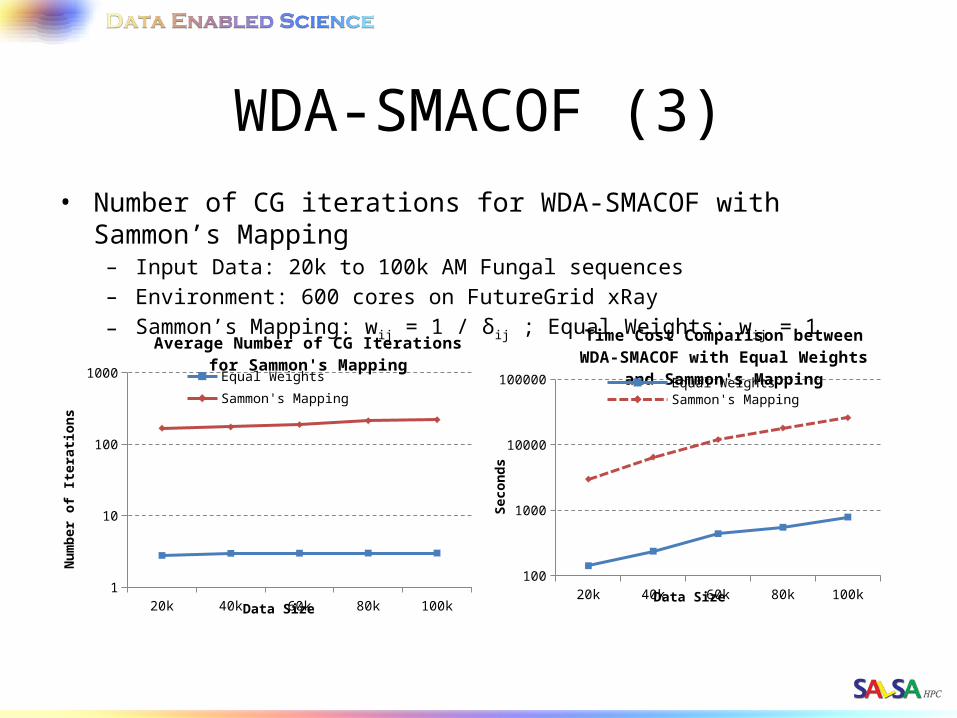
WDA-SMACOF (3)• Number of CG iterations for WDA-SMACOF with Sammon’s Mapping
– Input Data: 20k to 100k AM Fungal sequences– Environment: 600 cores on FutureGrid xRay– Sammon’s Mapping: wij = 1 / δij ; Equal Weights: wij = 1
20k 40k 60k 80k 100k100
1000
10000
100000
Time Cost Comparison between WDA-SMACOF with Equal Weights and
Sammon's MappingEqual WeightsSammon's Mapping
Data Size
Seco
nd
s
20k 40k 60k 80k 100k1
10
100
1000
Average Number of CG Iterations for Sammon's Mapping
Equal Weights Sammon's Mapping
Data Size
Nu
mb
er o
f Ite
rati
ons
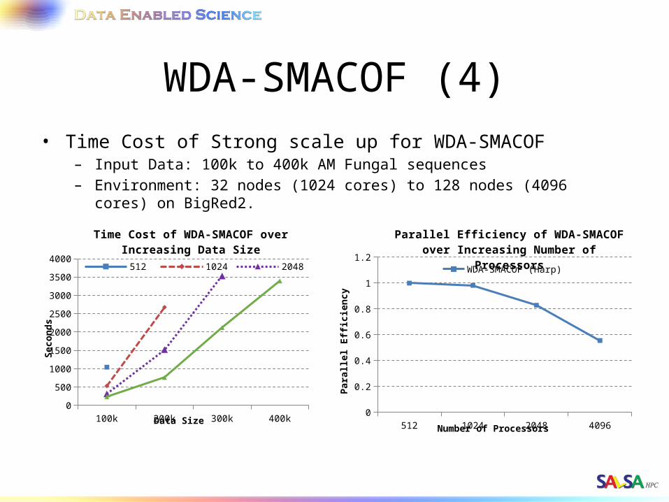
WDA-SMACOF (4)• Time Cost of Strong scale up for WDA-SMACOF
– Input Data: 100k to 400k AM Fungal sequences– Environment: 32 nodes (1024 cores) to 128 nodes (4096 cores) on BigRed2.
100k 200k 300k 400k0
500
1000
1500
2000
2500
3000
3500
4000
Time Cost of WDA-SMACOF over Increas-ing Data Size
512 1024 2048
Data Size
Seco
nd
s
512 1024 2048 40960
0.2
0.4
0.6
0.8
1
1.2
Parallel Efficiency of WDA-SMACOF over Increasing Number of Processors
WDA-SMACOF (Harp)
Number of Processors
Par
alle
l Eff
icie
ncy
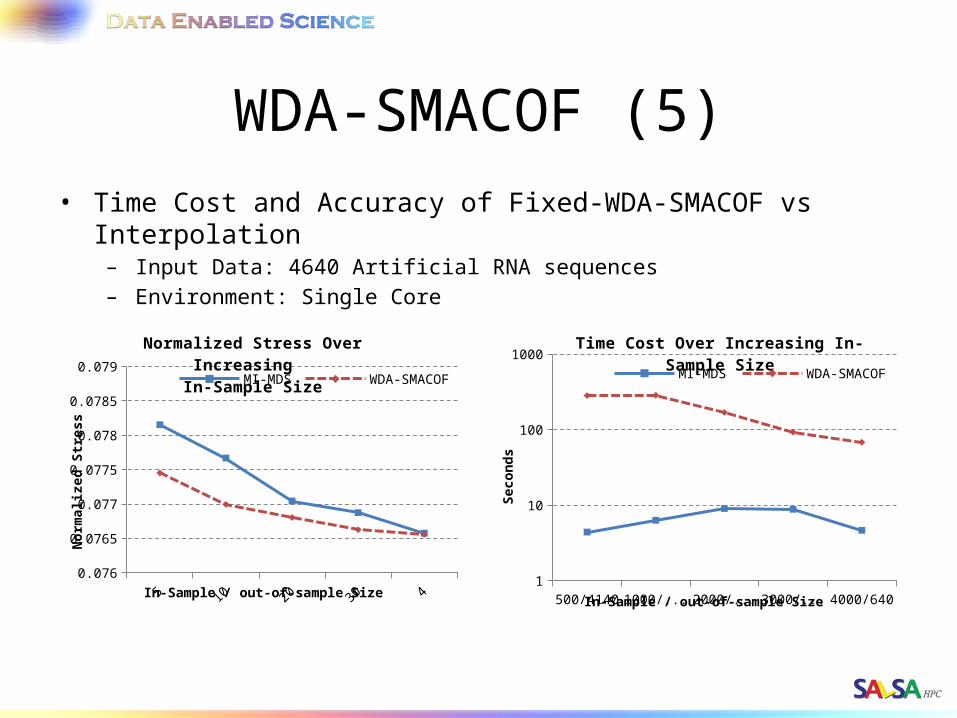
WDA-SMACOF (5)• Time Cost and Accuracy of Fixed-WDA-SMACOF vs Interpolation
– Input Data: 4640 Artificial RNA sequences– Environment: Single Core
500/4140 1000/3640 2000/2640 3000/1640 4000/6400.076
0.0765
0.077
0.0775
0.078
0.0785
0.079
Normalized Stress Over Increasing In-Sample Size
MI-MDS WDA-SMACOF
In-Sample / out-of-sample Size
Nor
mal
ized
Str
ess
500/4140 1000/3640 2000/2640 3000/1640 4000/6401
10
100
1000Time Cost Over Increasing In-Sample Size
MI-MDS WDA-SMACOF
In-Sample / out-of-sample Size
Seco
nd
s
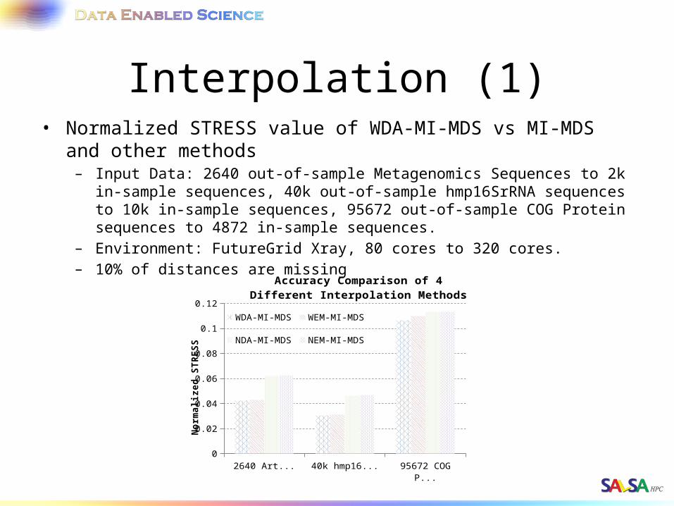
Interpolation (1)• Normalized STRESS value of WDA-MI-MDS vs MI-MDS and other
methods– Input Data: 2640 out-of-sample Metagenomics Sequences to 2k in-sample
sequences, 40k out-of-sample hmp16SrRNA sequences to 10k in-sample sequences, 95672 out-of-sample COG Protein sequences to 4872 in-sample sequences.
– Environment: FutureGrid Xray, 80 cores to 320 cores.– 10% of distances are missing
2640 Artificial RNA 40k hmp16SrRNA 95672 COG Protein0
0.02
0.04
0.06
0.08
0.1
0.12
Accuracy Comparison of 4 Different In-terpolation Methods
WDA-MI-MDS WEM-MI-MDS
NDA-MI-MDS NEM-MI-MDS
Nor
mal
ized
ST
RE
SS
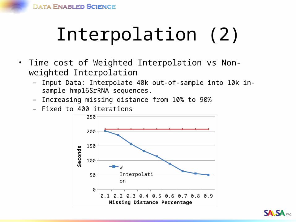
Interpolation (2)• Time cost of Weighted Interpolation vs Non-weighted Interpolation
– Input Data: Interpolate 40k out-of-sample into 10k in-sample hmp16SrRNA sequences.
– Increasing missing distance from 10% to 90%– Fixed to 400 iterations
0.1 0.2 0.3 0.4 0.5 0.6 0.7 0.8 0.90
50
100
150
200
250
W Interpolation
N Interpolation
Missing Distance Percentage
Seco
nds
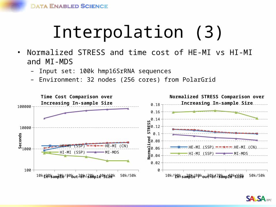
Interpolation (3)• Normalized STRESS and time cost of HE-MI vs HI-MI and MI-MDS
– Input set: 100k hmp16SrRNA sequences– Environment: 32 nodes (256 cores) from PolarGrid
10k/90k 20k/80k 30k/70k 40k/60k 50k/50k100
1000
10000
100000
Time Cost Comparison over Increasing In-sample Size
HE-MI (SSP) HE-MI (CN)
HI-MI (SSP) MI-MDS
In-sample / out-of-sample Size
Seco
nd
s
10k/90k 20k/80k 30k/70k 40k/60k 50k/50k0
0.02
0.04
0.06
0.08
0.1
0.12
0.14
0.16
0.18
Normalized STRESS Comparison over Increas-ing In-sample Size
HE-MI (SSP) HE-MI (CN)
HI-MI (SSP) MI-MDS
In-sample / out-of-sample Size
Nor
mal
ized
ST
RE
SS
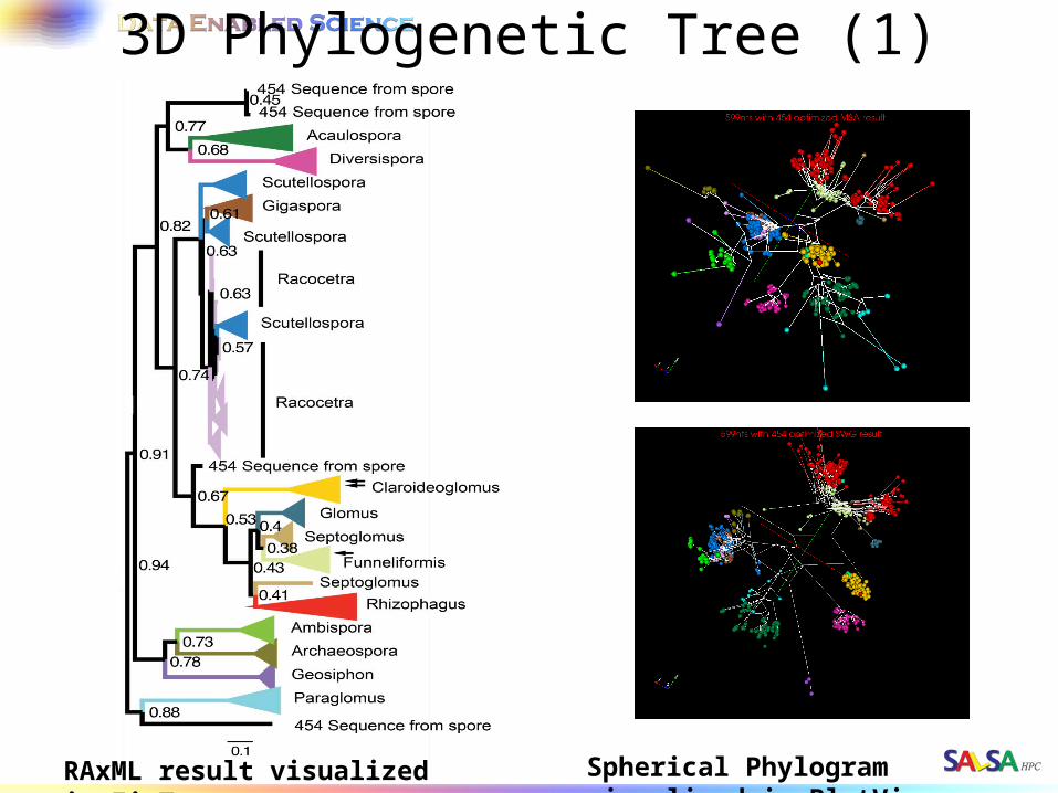
3D Phylogenetic Tree (1)
RAxML result visualized in FigTree. Spherical Phylogram visualized in PlotViz
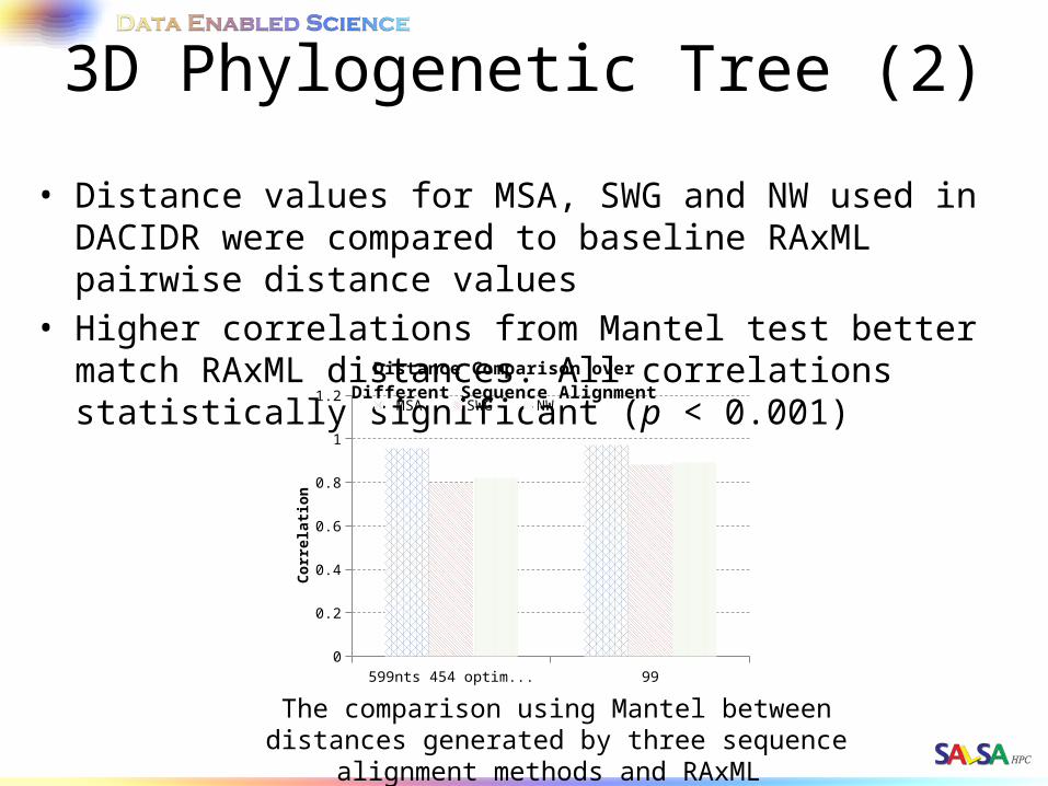
3D Phylogenetic Tree (2)
• Distance values for MSA, SWG and NW used in DACIDR were compared to baseline RAxML pairwise distance values
• Higher correlations from Mantel test better match RAxML distances. All correlations statistically significant (p < 0.001)
The comparison using Mantel between distances generated by three sequence alignment methods and RAxML
599nts 454 optimized 999nts0
0.2
0.4
0.6
0.8
1
1.2
Distance Comparison over Different Sequence Alignment
MSA SWG NW
Corr
elat
ion
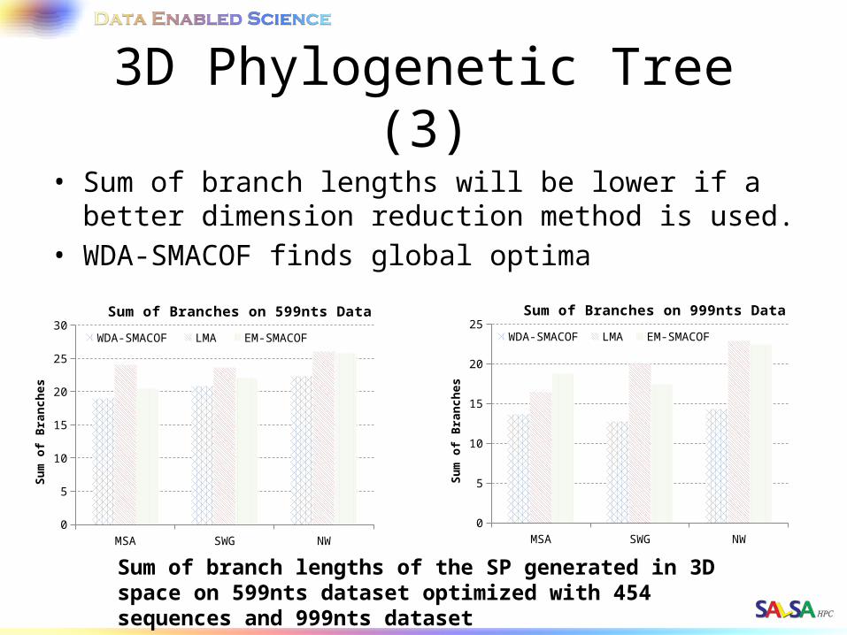
3D Phylogenetic Tree (3)• Sum of branch lengths will be lower if a better dimension
reduction method is used.• WDA-SMACOF finds global optima
Sum of branch lengths of the SP generated in 3D space on 599nts dataset optimized with 454 sequences and 999nts dataset
MSA SWG NW0
5
10
15
20
25
30Sum of Branches on 599nts Data
WDA-SMACOF LMA EM-SMACOF
Sum
of B
ran
ches
MSA SWG NW0
5
10
15
20
25Sum of Branches on 999nts Data
WDA-SMACOF LMA EM-SMACOF
Sum
of B
ran
ches
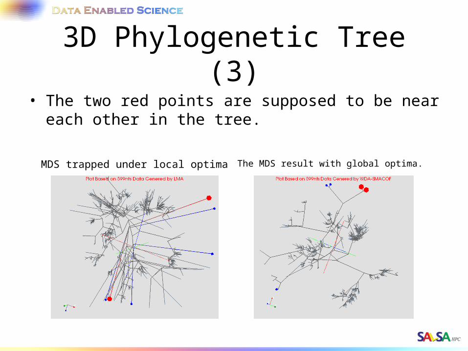
3D Phylogenetic Tree (3)• The two red points are supposed to be near each other in
the tree.
The MDS result with global optima.MDS trapped under local optima
Outline
• Motivation• Background and Related Work• Research Issues• Experimental Analysis• Conclusion and Futurework
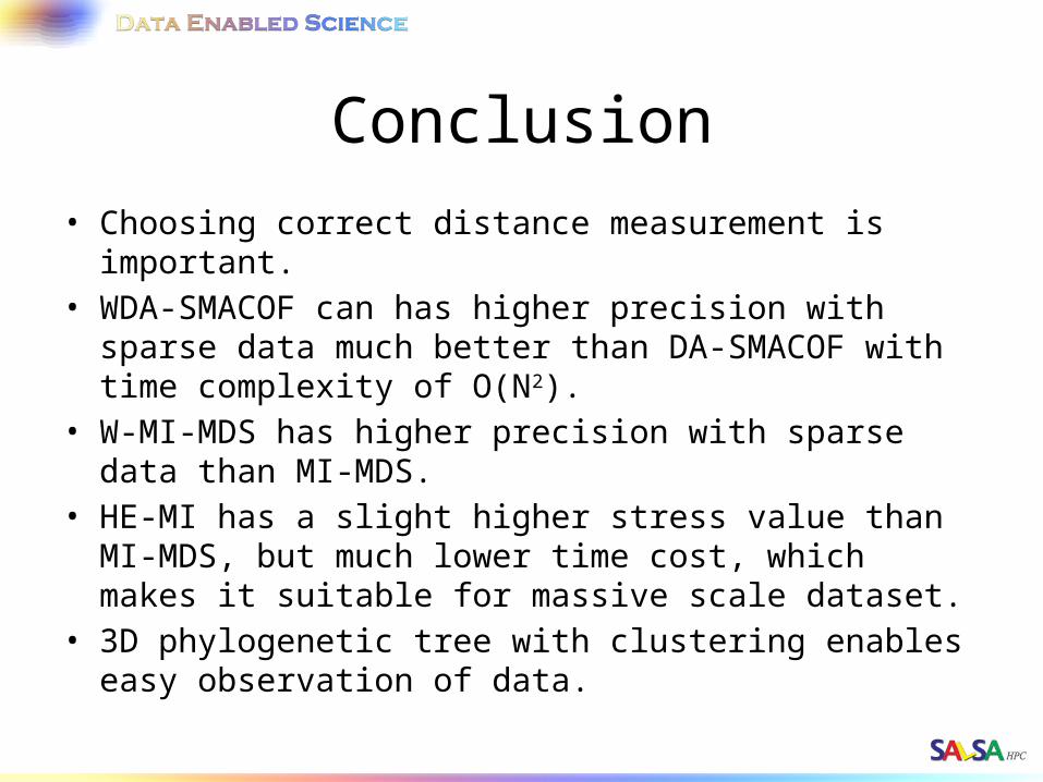
Conclusion• Choosing correct distance measurement is important.• WDA-SMACOF can has higher precision with sparse data
much better than DA-SMACOF with time complexity of O(N2).
• W-MI-MDS has higher precision with sparse data than MI-MDS.
• HE-MI has a slight higher stress value than MI-MDS, but much lower time cost, which makes it suitable for massive scale dataset.
• 3D phylogenetic tree with clustering enables easy observation of data.
Futurework• Hybrid Tree Interpolation
– Combine the usage of SSP-Tree and CN-Tree and possibly eliminates the weakness of both methods.
• Display Phylogenetic tree with million sequences• Enable faster execution of WDA-SMACOF with non-trivial
weights.– Need to investigate more about the CG iterations per SMACOF
iteration
• Write papers about new results, since WDA-SMACOF with Harp are so far best non-linear MDS.
• Phylogenetic tree with clustering and make it available.
Reference• Y Ruan, G House, S Ekanayake, U Schütte, JD Bever, H Tang, G Fox , Integration of Clustering
and Multidimensional Scaling to Determine Phylogenetic Trees as Spherical Phylograms Visualized in 3 Dimensions, Proceedings of C4Bio 2014, 26-29
• Yang Ruan, Geoffrey Fox. A Robust and Scalable Solution for Interpolative Multidimensional Scaling with Weighting. Proceedings of IEEE eScience 2013, Beijing, China, Oct. 22-Oct. 25, 2013. (Best Student Innovation Award)
• Yang Ruan, Saliya Ekanayake, et al. DACIDR: Deterministic Annealed Clustering with Interpolative Dimension Reduction using a Large Collection of 16S rRNA Sequences. Proceedings of ACM-BCB 2012, Orlando, Florida, ACM, Oct. 7-Oct. 10, 2012.
• Yang Ruan, Zhenhua Guo, et al. HyMR: a Hybrid MapReduce Workflow System. Proceedings of ECMLS’12 of ACM HPDC 2012, Delft, Netherlands, ACM, Jun. 18-Jun. 22, 2012.
• Adam Hughes, Yang Ruan, et al. Interpolative multidimensional scaling techniques for the identification of clusters in very large sequence sets, BMC Bioinformatics 2012, 13(Suppl 2):S9.
• Jong Youl Choi, Seung-Hee Bae, et al. High Performance Dimension Reduction and Visualization for Large High-dimensional Data Analysis. to appear in the Proceedings of the The 10th IEEE/ACM International Symposium on Cluster, Cloud and Grid Computing (CCGrid 2010), Melbourne, Australia, May 17-20 2010.
• Seung-Hee Bae, Jong Youl Choi, et al. Dimension Reduction Visualization of Large High-dimensional Data via Interpolation. to appear in the Proceedings of The ACM International Symposium on High Performance Distributed Computing (HPDC), Chicago, IL, June 20-25 2010.

Questions?

Backup Slides
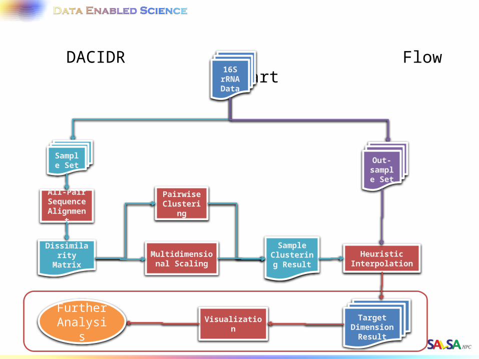
DACIDR Flow Chart16S rRNA Data
All-Pair Sequence Alignment
Heuristic Interpolation
Pairwise Clustering
Multidimensional Scaling
Dissimilarity Matrix
Sample Clustering
Result
Target Dimension
Result
Visualization
Out-sample
Set
Sample Set
Further Analysis
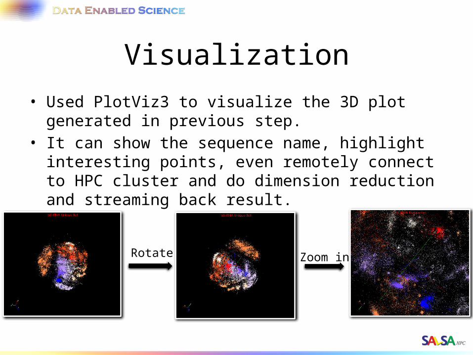
Visualization• Used PlotViz3 to visualize the 3D plot generated in previous
step.• It can show the sequence name, highlight interesting points,
even remotely connect to HPC cluster and do dimension reduction and streaming back result.
Zoom inRotate
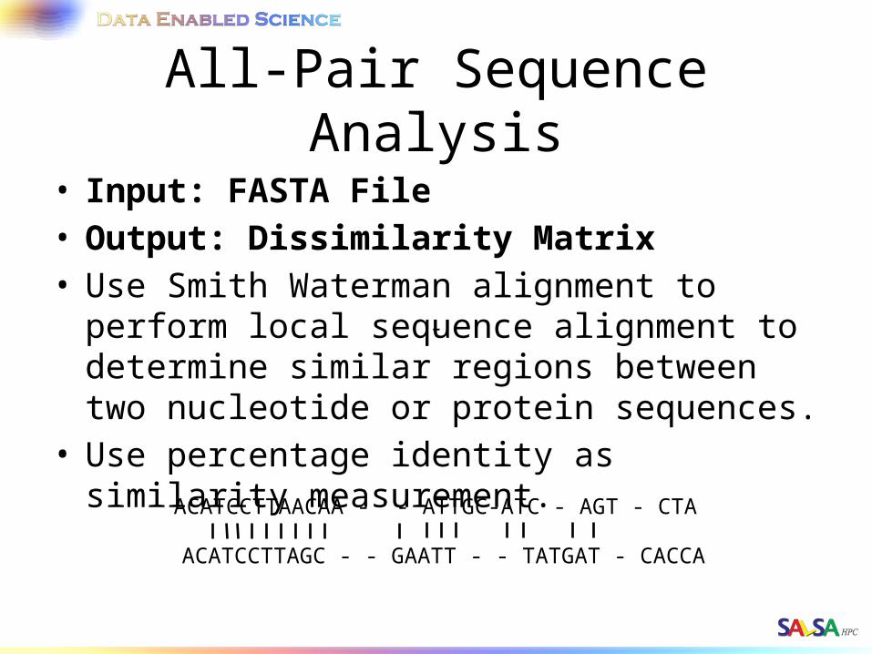
All-Pair Sequence Analysis• Input: FASTA File• Output: Dissimilarity Matrix• Use Smith Waterman alignment to perform local
sequence alignment to determine similar regions between two nucleotide or protein sequences.
• Use percentage identity as similarity measurement.
ACATCCTTAACAA - - ATTGC-ATC - AGT - CTA
ACATCCTTAGC - - GAATT - - TATGAT - CACCA
-
Deterministic Annealing• Deterministic Annealing clustering is a robust pairwise
clustering method.• Temperature corresponds to pairwise distance scale and one
starts at high temperature with all sequences in same cluster. As temperature is lowered one looks at finer distance scale and additional clusters are automatically detected.
• Multidimensional Scaling is a set of dimension reduction techniques. Scaling by Majorizing a Complicated Function (SMACOF) is a classic EM method and can be parallelized efficiently
• Adding temperature from DA can help prevent local optima problem.
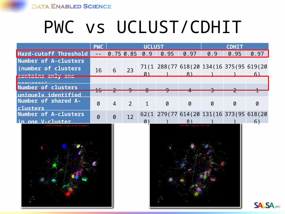
PWC vs UCLUST/CDHIT
PWC UCLUST
PWC UCLUST CDHITHard-cutoff Threshold -- 0.75 0.85 0.9 0.95 0.97 0.9 0.95 0.97Number of A-clusters (number of clusters contains only one sequence)
16 6 23 71(10) 288(77) 618(208) 134(16) 375(95) 619(206)
Number of clusters uniquely identified 16 2 9 8 9 4 3 2 1
Number of shared A-clusters 0 4 2 1 0 0 0 0 0Number of A-clusters in one V-cluster 0 0 12 62(10) 279(77) 614(208) 131(16) 373(95) 618(206)
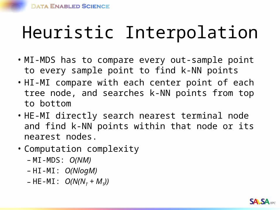
Heuristic Interpolation• MI-MDS has to compare every out-sample point to
every sample point to find k-NN points• HI-MI compare with each center point of each tree
node, and searches k-NN points from top to bottom• HE-MI directly search nearest terminal node and find
k-NN points within that node or its nearest nodes.• Computation complexity
– MI-MDS: O(NM)– HI-MI: O(NlogM)– HE-MI: O(N(NT + MT))
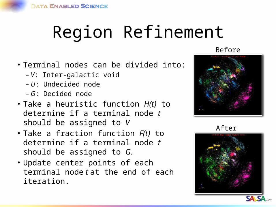
Region Refinement
• Terminal nodes can be divided into:– V: Inter-galactic void– U: Undecided node– G: Decided node
• Take a heuristic function H(t) to determine if a terminal node t should be assigned to V
• Take a fraction function F(t) to determine if a terminal node t should be assigned to G.
• Update center points of each terminal node t at the end of each iteration.
Before
After
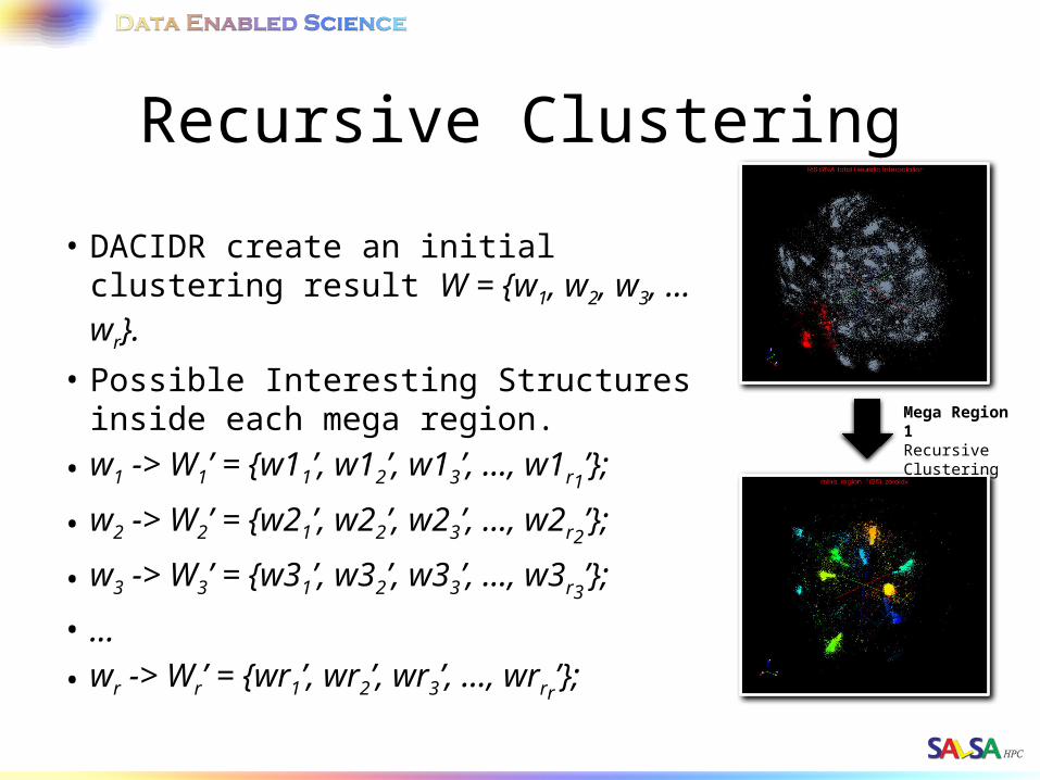
Recursive Clustering
• DACIDR create an initial clustering result W = {w1, w2, w3, … wr}.
• Possible Interesting Structures inside each mega region.
• w1 -> W1’ = {w11’, w12’, w13’, …, w1r1’};
• w2 -> W2’ = {w21’, w22’, w23’, …, w2r2’};
• w3 -> W3’ = {w31’, w32’, w33’, …, w3r3’};
• …• wr -> Wr’ = {wr1’, wr2’, wr3’, …, wrrr
’};
Mega Region 1Recursive Clustering
Multidimensional Scaling• Input: Dissimilarity Matrix• Output: Visualization Result (in 3D)• MDS is a set of techniques used in dimension reduction.• Scaling by Majorizing a Complicated Function (SMACOF) is a
fast EM method for distributed computing.• DA introduce temperature into SMACOF which can eliminates
the local optima problem.
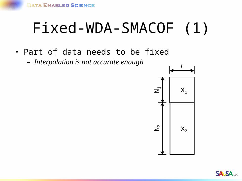
Fixed-WDA-SMACOF (1)• Part of data needs to be fixed
– Interpolation is not accurate enough
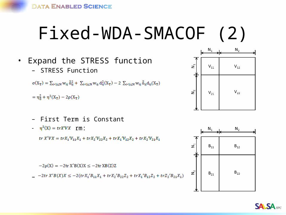
Fixed-WDA-SMACOF (2)• Expand the STRESS function
– STRESS Function
– First Term is Constant– Second Term:
– Third Term:
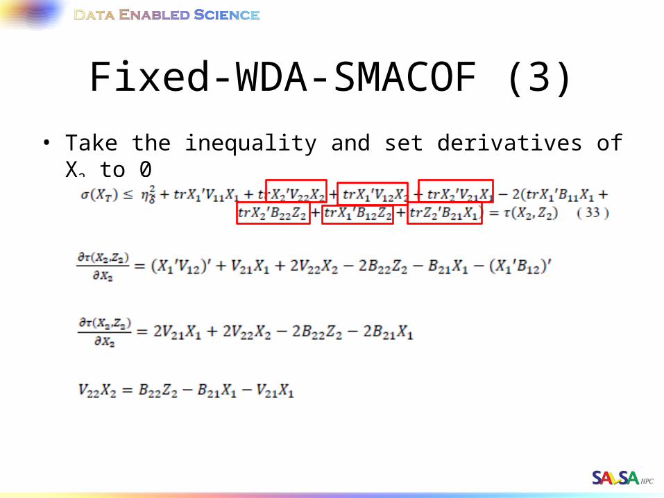
Fixed-WDA-SMACOF (3)
• Take the inequality and set derivatives of X2 to 0