Your Dreams May Come True with MTP2€¦ · Your Dreams May Come True with MTP2... Caroline Uhler (MIT) Joint work with Shaun Fallat, Ste en Lauritzen, Kayvan Sadeghi, Nanny Wermuth,

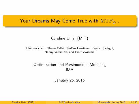
Your Dreams May Come True with MTP2...

Caroline Uhler (MIT)

Joint work with Shaun Fallat, Steffen Lauritzen, Kayvan Sadeghi,Nanny Wermuth, and Piotr Zwiernik

Optimization and Parsimonious ModelingIMA

January 26, 2016

Caroline Uhler (MIT) MTP2 distributions Minneapolis, January 2016 1 / 18

Problem

Given large data sets for example from medical tests or IQ tests,determine a sparse graph that describes the dependencies between thevariables.

1/25/16

pro

ble

ms

1

p

2

...

1 n2 ...individuals

mea

sure

men

ts

1

p

2

...

1 n2 ...patients

Two common approaches:

Machine Learning: Graphical lasso

Applied Statistics: Chow-Liu and subsequent stepwise selection


Overview

1. MTP2 distributions

2. Properties of MTP2 distributions related to sparsity

3. Models that imply MTP2

4. Maximum likelihood estimation under MTP2


Positive dependence and MTP2 distributions

A distribution (i.e. density function) p on X is multivariate totallypositive of order 2 (MTP2) if

p(x)p(y) ≤ p(x ∧ y)p(x ∨ y) for all x , y ∈ X ⊂ Rm.

A random vector X is positively associated if for any non-decreasingfunctions φ, ψ : Rm → R

cov{φ(X ), ψ(X )} ≥ 0.

Theorem (FortuinKasteleynGinibre inequality, 1971)

MTP2 implies positive association.


Discrete and Gaussian MTP2 distribution

Example: Binary vector X = (X1,X2,X3) ∈ {0, 1}3 is MTP2 if and only ifp001p110 ≤ p000p111 p010p101 ≤ p000p111 p100p011 ≤ p000p111

p011p101 ≤ p001p111 p011p110 ≤ p010p111 p101p110 ≤ p100p111

p001p010 ≤ p000p011 p001p100 ≤ p000p101 p010p100 ≤ p000p110

Theorem (Horn and Johnson, 1991)

A multivariate Gaussian distribution p(x ; θ) is MTP2 if and only if theinverse covariance matrix θ is an M-matrix, that is

θij ≤ 0 for all i 6= j .

Theorem (Karlin and Rinott, 1980)

If p(x) > 0 and p is MTP2 for any pair of coordinates when the others areheld constant, then p is MTP2.


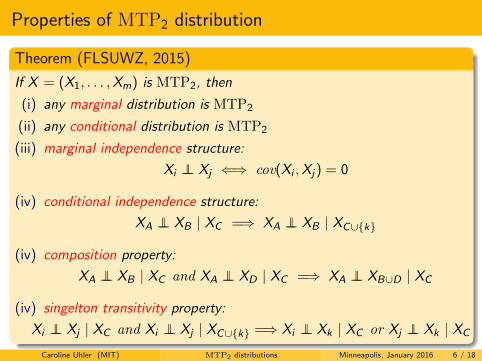
Properties of MTP2 distribution

Theorem (FLSUWZ, 2015)

If X = (X1, . . . ,Xm) is MTP2, then

(i) any marginal distribution is MTP2

(ii) any conditional distribution is MTP2

(iii) marginal independence structure:

Xi ⊥⊥ Xj ⇐⇒ cov(Xi ,Xj) = 0

(iv) conditional independence structure:

XA ⊥⊥ XB | XC =⇒ XA ⊥⊥ XB | XC∪{k}

(iv) composition property:

XA ⊥⊥ XB | XC and XA ⊥⊥ XD | XC =⇒ XA ⊥⊥ XB∪D | XC

(iv) singelton transitivity property:

Xi ⊥⊥ Xj | XC and Xi ⊥⊥ Xj | XC∪{k} =⇒ Xi ⊥⊥ Xk | XC or Xj ⊥⊥ Xk | XC


Occurrence of MTP2 distributions

MTP2 contraints appear to be extremely restrictive:

3-dim. Gaussian distributions: about 5% are MTP2

4-dim. Gaussian distributions: about 0.09% are MTP2

3-dim. binary distributions: about 2% are MTP2

4-dim. binary distributions: about 0% are MTP2

Constraints are less restrictive with additional Markov structure!

For 3-dim. Gaussian distributions:

if 1 ⊥⊥ 2 | 3: 25% are MTP2,

if in addition 1 ⊥⊥ 3 | 2: 50% are MTP2,

if 1 ⊥⊥ 2 ⊥⊥ 3: 100% are MTP2.


Example: EPH-gestosis

Dataset collected 40 years ago in a study on “Pregnancy and ChildDevelopment” by the German Research Foundation and recently analyzedby Wermuth and Marchetti (2014).

EPH-gestosis: disease syndrome for pregnant women; three symptoms

edema (high body water retention)

proteinuria (high amounts of urinary proteins)

hypertension (elevated blood pressure)

Observed counts:[n000 n010 n001 n011

n100 n110 n101 n111

]=

[3299 107 1012 58

78 11 65 19

].

This sample distribution is MTP2!


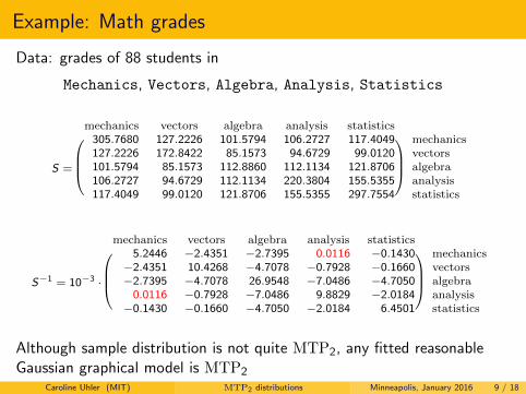
Example: Math grades

Data: grades of 88 students in

Mechanics, Vectors, Algebra, Analysis, Statistics

S =

mechanics vectors algebra analysis statistics

305.7680 127.2226 101.5794 106.2727 117.4049 mechanics127.2226 172.8422 85.1573 94.6729 99.0120 vectors101.5794 85.1573 112.8860 112.1134 121.8706 algebra106.2727 94.6729 112.1134 220.3804 155.5355 analysis117.4049 99.0120 121.8706 155.5355 297.7554 statistics

S−1 = 10−3 ·

mechanics vectors algebra analysis statistics

5.2446 −2.4351 −2.7395 0.0116 −0.1430 mechanics−2.4351 10.4268 −4.7078 −0.7928 −0.1660 vectors−2.7395 −4.7078 26.9548 −7.0486 −4.7050 algebra

0.0116 −0.7928 −7.0486 9.8829 −2.0184 analysis−0.1430 −0.1660 −4.7050 −2.0184 6.4501 statistics

Although sample distribution is not quite MTP2, any fitted reasonableGaussian graphical model is MTP2


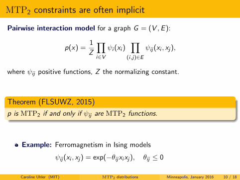
MTP2 constraints are often implicit

Pairwise interaction model for a graph G = (V ,E ):

p(x) =1

Z

∏i∈V

ψi (xi )∏

(i ,j)∈Eψij(xi , xj),

where ψij positive functions, Z the normalizing constant.

Theorem (FLSUWZ, 2015)

p is MTP2 if and only if ψij are MTP2 functions.

Example: Ferromagnetism in Ising models

ψij(xi , xj) = exp(−θijxixj), θij ≤ 0


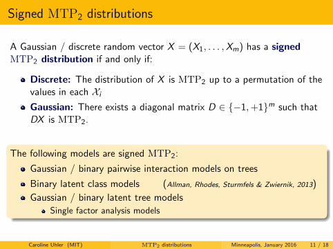
Signed MTP2 distributions

A Gaussian / discrete random vector X = (X1, . . . ,Xm) has a signedMTP2 distribution if and only if:

Discrete: The distribution of X is MTP2 up to a permutation of thevalues in each Xi

Gaussian: There exists a diagonal matrix D ∈ {−1,+1}m such thatDX is MTP2.

The following models are signed MTP2:

Gaussian / binary pairwise interaction models on trees

Binary latent class models (Allman, Rhodes, Sturmfels & Zwiernik, 2013)

Gaussian / binary latent tree models

Single factor analysis models


ML Estimation for Gaussian graphical models

Primal: Max-Likelihood: Dual: Min-Entropy: G = (V ,E )


maximize✓⌫0

log det(✓) � trace(✓S)

subject to ✓uv = 0, 8 uv /2 E , u 6= v .

minimize⌃⌫0

� log det(⌃) � m

subject to ⌃uv = Suv , 8 uv 2 E , and u = v .



maximize✓⌫0


subject to ✓uv = 0, 8 uv /2 E , u 6= v .

minimize⌃⌫0


subject to ⌃uv = Suv , 8 uv 2 E , and u = v .


Concentration matrices: Covariance matrices:

GeometryGeometry


ML Estimation for Gaussian MTP2 distributions

Primal: Max-Likelihood: Dual: Min-Entropy:


maximize✓⌫0


subject to ✓uv 0, 8 u 6= v .

minimize⌃⌫0


subject to ⌃vv = Svv , ⌃uv � Suv .



maximize✓⌫0


subject to ✓uv 0, 8 u 6= v .

minimize⌃⌫0


subject to ⌃vv = Svv , ⌃uv � Suv .


Theorem

The MLE based on S exists if and only if there exists Σ � 0 with Σ ≥ S.It is then equal to the unique element θ̂ = Σ̂−1 � 0 that satisfies thefollowing system of equations and inequalities

(a) Primal feasibility: θ̂uv ≤ 0 ∀u 6= v ,

(b) Dual feasibility: Σ̂vv − Svv = 0 ∀v , Σ̂uv − Suv ≥ 0 ∀u 6= v

(c) Complimentary slackness: (Σ̂uv − Suv ) θ̂uv = 0 ∀u 6= v.

Note: We get sparsity for free!!



Theorem (Slawski and Hein, 2015)

The MLE in a Gaussian MTP2 model exists with probability 1 when n ≥ 2.

Theorem (LUZ, 2016)

Let S be a sample correlation matrix and θ̂ the MLE of the concentrationmatrix in the Gaussian MTP2 model. Let GMST (S) be the maximalspanning tree of S and G (θ̂) the concentration graph. Then

GMST (S) ⊂ G (θ̂).

Algorithm: Input: Sample correlation matrix SOutput: Graph under Gaussian signed MTP2 model

Let D ∈ {−1, 1}p diagonal s.t. Chow-Liu tree of DSD is positive

Compute MLE Σ̂ based on DSD under Gaussian MTP2 model

Output G (Σ̂−1)


Example: Carcass

344 measurements of the thickness of meat and fat layers at differentlocations of a slaughter pig

S−1 =

Fat11 Meat11 Fat12 Meat12 Fat13 Meat13

0.40 0.04 −0.23 −0.07 −0.19 0.05 Fat110.04 0.15 −0.01 −0.06 −0.05 −0.06 Meat11

−0.23 −0.01 0.51 0.07 −0.23 −0.05 Fat12−0.07 −0.06 0.07 0.14 −0.00 −0.09 Meat12−0.19 −0.05 −0.23 −0.00 0.54 0.03 Fat13

0.05 −0.06 −0.05 −0.09 0.03 0.16 Meat13

S =

Fat11 Meat11 Fat12 Meat12 Fat13 Meat13

11.34 0.74 8.42 2.06 7.66 −0.76 Fat110.74 32.97 0.67 35.94 2.01 31.97 Meat118.42 0.67 8.91 0.31 6.84 −0.60 Fat122.06 35.94 0.31 51.79 2.18 41.47 Meat127.66 2.01 6.84 2.18 7.62 0.38 Fat13

−0.76 31.97 −0.60 41.47 0.38 41.44 Meat13

Fat11

Meat11Fat12

Meat12

Fat13 Meat13

Fat11

Meat11Fat12

Meat12

Fat13 Meat13

Under MTP2 constraint Using glasso


Example: BodyFat

241 observations on 15 variables: age, weight, height, percentage of bodyfat, body density, and the circumferences of various body parts.

Density

BodyFat

Age

WeightHeight

Neck

Chest

Abdomen

Hip

Thigh

KneeAnkle Biceps

Forearm

Wrist

Density

BodyFat

Age

WeightHeight

Neck

Chest

Abdomen

Hip

Thigh

KneeAnkle Biceps

Forearm

Wrist

Under MTP2 constraint Using glasso


Conclusions and future work

MTP2 constraints reflect real processes and models

ferromagnetism

latent class models with positive associations

latent Gaussian/binary tree models

they lead to some beautiful theory (exponential families, convexity,combinatorics, semialgebraic geometry)

they are useful in high-dimensional settings


References

Fallat, Lauritzen, Sadeghi, Uhler, Wermuth, and Zwiernik: Totalpositivity in Markov structures (arXiv:1510.01290)

Lauritzen, Uhler, and Zwiernik: Totally positive exponential familiesand graphical models (on the arXiv shortly)

!"#$%&'()*+*,-.**/#("012$02"'*32#))024)5*)'%06'&040"'*%2"$07*

89%:('"0945*246*8941'7*2(;'<$208*;'9%'"$=*>?@!/*AB5*BCDCE

,-.*3'9%'"$=*9&*%270%#%*(0F'(0G996*')"0%2"094*04*32#))024*;$2:G082(*

%96'()*>G9:'&#((=*94*"G'*2$H01*<=*!#462=E

IG246$2)'F2$245*!G2G5*,-*?)=%:"9"08)*9&*%270%#%*(0F'(0G996*

')"0%2"094*04*32#))024*8=8(')*>04*:$9;$'))E

!"#$%&'()

*


Documents

Your Dreams May Come True with MTP2€¦ · Your Dreams May Come True with MTP2... Caroline Uhler (MIT) Joint work with Shaun Fallat, Ste en Lauritzen, Kayvan Sadeghi, Nanny Wermuth,