Z50

RESPONSE OF NONLINEAR STRUCTURES TO DETERMINISTIC

AND RANDOM EXCITATIONS

bv

Sami: Jawdat Serhan

Dissertation submitted to the Faculty of the

Virginia Polytechnic Institute and State University

in partial fulfilment of the requirements for the degree of

DOCTOR OF PHILOSOPHY

in

Engineering Mechanics

APPROVED: A

Ali . Nayfeh, Chaiäman

Dean T. Mook Mahendra P. Singh

•

L~»GeraldN. Cloug Luther G. Kraige

i

Ioannis M. Besieris

March 1989

Blacksburg, Virginia

RESPONSE OF NONLINEAR STRUCTURES TO DETERMINISTIC AND

RANDOM EXCITATIONS

by

Samir J. Serhan

Ali H. Nayfeh, Chairman

Engineering Mechanics

(ABSTRACT)

Three methods are developed to study the response of nonlinear

systems to combined deterministic and stochastic excitations. They are

a second-order closure method, a generalized method of equivalent

linearization, and a reduced non-Gaussian closure scheme. Primary

resonances of single- and two—degree-of-freedom systems in the presence

of different internal (autoparametric) resonances are investigated. we

propose these methods to overcome some of the limitations of the

existing methods of solution and explain some observed experimental

results in the context of the response of randomly excited nonlinear

systems. These include non—Gaussian responses, broadening effects, and

shift in the resonant frequency. when available, the results of these

methods are compared with those obtained by using the exact stationary

solutions of the Fokker-Planck-Kolmogorov equation. It is found that

the presence of the nonlinearities bend the frequency-response curves

and this causes multi-valued regions for the mean-square responses. The

multi-valuedness is responsible for a jump phenomenon. The results show

that for some range of parameters, noise can expand the stability region

of the mean response. As applications, we study the response of a

shallow arch, a string, and a hinged-clamped beam to random excitations.

iv

TABLE DF CONTENTS

Page

ACKNOWLEDGEMENTS iv

TABLE DF CONTENTS v

CHAPTER 1 INTRDDUCTIDN 1

1.1 Scope of Work 1

1.2 Applications 4

1.3 System Characterization 4

1.3.1 Excitations 4

1.3.2 Nonlinearities 5

1.4 Methods of Solution 6

1.4.1 Markov Methods 7

1.4.2 Sequence of Interative Solutions 15

1.4.3 Stochastic Averaging 16

1.4.4 Series Expansions 22

1.4.5 Random—walk Analogy 25

1.4.6 Moment Closures 26

1.4.7 Equivalent or Statistical Linearization 27

1.4.8 Perturbation Methods 31

1.4.9 Digital- and Analog—Computer Simulation 32

v

CHAPTER 2 A SECON0—ORDER CLOSURE METHOD 34

2.1 Introduction 35

2.2 The Method of Multiple Scales 35

2.3 Linearization Method 37

2.3.1 Nonstationary—Random-Amplitude Sinusoids 41

2.3.2 white Noise 43

2.4 Second-Order Closure Method 44

2.5 Semi-Linearization Method 50

2.6 Equivalent Linearization for Non-Zero Mean

Random Excitations 52

2.7 Numerical Results 54

2.6 ConclusionsA

60

CHAPTER 3 A GENERALIZED METHOD OF EQUIVALENT LINEARIZATION 61

3.1 Introduction 61

3.2 Limitations of the Method of Equivalent

Linearization 69

3.2.1 Primary Resonance 70

3.2.2 Superharmonic Resonance of Order-Three 70

3.2.3 Subharmonic Resonance of Order One—Third 71

3.3 Proposed Method 72

3.4 Examples and Accuracy 74

3.4.1 The Ouffing Oscillator 74

3.4.2 The Van der Pol—Rayleigh Oscillator 82

3.5 Conclusions 86

vi

CHAPTER 4 NONLINEAR RANDOM COUPLED MOTIONS OF STRUCTURAL

ELEMENTS WITH QUADRATIC NONLINEARITIES 88

4.1 Introduction 88

4.2 The Method of Multiple Scales 92

4.3 Analysis 96

4.4 Results and Conclusions 100

CHAPTER 5 CUMULANT-NEGLECT CLOSURE FOR SYSTEMS WITH MOOAL

INTERACTION 103

5.1 Introduction 104

5.2 Closure Schemes via the Markov Procedure 106

5.3 Non-Gaussian Closure 109

5.4 Two-to—0ne Internal Resonance with

Application to an Arch 111

5.5 0ne—to—0ne Internal Resonance with

Application to a String 116

5.6 Three-to-One Internal Resonance with

Application to a Hinged-Clamped Beam 119

5.7 Conclusions 122

CHAPTER 6 CONCLUSIONS AND RECOMMENDATIONS FOR FUTURE WORK 124

REFERENCES 129

APPENDICES

Appendix I: The Matrix B and Vector 0156

Appendix II: Method of Averaging 157

Appendix III: Two-to-One Internal Resonance;

Zero-Response Moments 159

vii

Appendix IV: 0ne—to-One Internal Resonance;

Zero—Response Moments 160

Appendix V: Three—to-0ne Internal Resonance;

Zero-Response Moments 161

FIGURES 162

VITA 208

viii·

ICHAPTER 1

INTRODUCTION

1.1 Scope of work A

This dissertation presents the research performed towards the

analysis and development of new methods for predicting the response of

nonlinear systems to deterministic and stochastic excitations. These

are a second-order closure method, a generalized method of equivalent

linearization, and a reduced non-Gaussian closure scheme. In the

former, we take the following typical steps. First, we use the method

of multiple scales to determine the equations describing the modulation

of the amplitude and phase of the narrow-band response with time.

Second, we separate the averaged equations into mean and fluctuating

components. Third, we use these equations to obtain closed-form

expressions for the stationary mean and mean-square response. The

results show that the presence of the nonlinearity bends the frequency-

response curves and this causes multi-valued regions for the mean-square

responses. The multi-valuedness is responsible for a jump phenomenon.

The results show that for some range of parameters, noise can expand the

stability region of the mean response.

The method of equivalent linearization has the widest range of

applicability for solving nonlinear stochastic problems. It is based on

replacing the nonlinear governing equations by equivalent linear

equations whose solution furnishs an approximate solution to the

nonlinear response. In achieving this goal, the method of equivalent

linearization creates many limitations and overlooks many interesting

1

phenomena caused by the nonlinearity. In Chapter 3 we propose a

generalized method of equivalent linearization to overcome some of these

limitations and explain some experimental results in the context of the

response of randomly excited nonlinear structures. These include non-

Gaussian responses, broadening effects, and shifts in the resonant

frequencies. The proposed approach is illustrated by investigating the

response of a class of nonlinear systems to a Gaussian white noise and a

superharmonic narrow-band random excitation of order-three. The results

of this method are compared with those obtained by using the method of

equivalent linearization and some exact stationary solutions of the

Fokker—Planck-Kolmogorov equation.

The second—order closure method is direct and can be easily

extended to the case of multi—degree—of-freedom systems. As an

application, the second-order closure method is used to determine the

forced response of a two-degree—of—freedom system with quadratic

nonlinearities in Chapter 4. The excitation is taken to be the sum of a

deterministic harmonic component and a random component. The latter may

be either white noise or a narrow-band random excitation. The case of

primary resonance of the second mode in the presence of a two—to—one

internal (autoparametric) resonance is investigated. Contrary to the

results predicted by the linear analysis, the nonlinear analysis reveals

that under a narrow-band random excitation of the second mode, it may

saturate and spill the energy over to the indirectly excited first mode

due to the autoparametric resonance.

2

In Chapter 5 three closure techniques via the Markov vector

procedure are used to determine the response moments of a two-degree-of-

freedom system with quadratic and cubic nonlinearities. They are the

Gaussian, non-Gaussian, and reduced non—Gaussian closure techniques.

The cases of two-to-one, one-to-one, and three—to—one internal

resonances are investigated. The system is externally excited by a

zero-mean Gaussian white noise. Ito stochastic calculus is used to

derive a heirarchy of first—order differential equations governing the

modulation of the response moments with time. The Gaussian closure

scheme generates I4 coupled equations for the first- and second-order

response moments and the non—Gaussian closure scheme, based on setting

the fifth- and sixth—order cumulants equal to zero, generates 69 coupled

equations for the first-order through the fourth-order response

moments. The method of multiple scales is used to describe the nature

of the response and its characteristics. This information is utilized

to drastically reduce the number of the response—moment equations

generated by the non—Gaussian closure scheme. The results reveal major

a discrepancies between the Gaussian and non-Gaussian closure schemes.

Close to internal resonance, the response displays an energy exchange

between the two internally resonant modes. The response, however, does

not display the saturation phenomenon for the case of two-to-one

internal resonances. The results are applied to a shallow arch, a

string, and a hinged-clamped beam.

3

1.2 Applications

Most of nature's excitations exhibit randomly fluctuating

characteristics and contain a wide spectrum of frequencies that may

result in severe vibrations. Due to the highly unpredictable trends of

these natural hazard excitations in a deterministic sense, stochastic

processes may be used to describe these excitations, which are

completely characterized by probability-density functions or certain

statistical measures. This explains the wide scope of applications of

random vibrations to the solution of practical engineering problems,

such as strong motion earthquakes (earthquake engineering), the motion

of a ship in a confused sea (ocean engineering), road roughness

(transportation engineering), the motion of an aircraft or a missile

through a turbulent air (aeronautical engineering), computing machines,

the design of particle accelerators, time measurements and coherent

radar detection (statistical radio engineering), gusty winds (wind

engineering), thermionic noise, and the effect of sea waves on offshore

structures (civil engineering).

1.3 System Characterization

1.3.1 Excitations

An excitation is described as an ideal excitation if it has enough

power so that there will be no feedback from the system to the source of

excitation. Both ideal and nonideal excitations are described as random

excitations if it is only possible to characterize them by statistical

measures. However, random and deterministic excitations could be

4

categorized as parametric or nonparametric (external) excitations.

Parametric excitations appear as variable coefficients in the

differential equations of motion and/or the boundary conditions; they

may be caused by axial loads. A common problem for systems excited by

parametric forces is their instability. A nonlinear model will limit

the unlimited exponential amplitude of the response predicted by the

linear model. A random excitation is said to be strict-sense stationary

if its statistical characteristics are invariant under time shifts and

wide-sense stationary if its mean is constant and its auto—correlation

function depends only on the separation time.

1.3.2 Nonlinearities

Dynamical systems subjected to random excitations exhibit

nonlinearities for sufficiently large motions [1,2]. The sources of the

nonlinearities may be material (nonlinear elasticity, perfect

plasticity, strain hardening, etc.), geometric (excessive displacements,

curvature, etc.), damping (dry friction, hysteretic damping, etc.), and

inertia. The output of a linear system to a Gaussian input is

Gaussian. Unignorable nonlinearities in the system may deviate the

output from being normal (Gaussian distribution). The deviated output

yields different probability-density functions that influence the

investigation of the failure criteri of such systems [3-5]. Linear

problems can be solved exactly by a variety of techniques, see for

example, Nang and Uhlenbeck [6] and Bharucha-Reid [7]; a comprehensive

treatment is available in standard textbooks [8-10]. Many techniques

5

have been developed to determine the response of nonlinear systems to

random excitations. Section 1.4 provides a brief review of these

techniques. Q

1.4 Methods of Solution

The early start and development of the problem of nonlinear random

vibration were completely formed and mixed up with the contributions and

formulation of the solution of the Fokker-Planck-Kolmogorov (in short,

FPK) equation.

The general problem of random vibration has been included in the

literature for many years through the study of Brownian motion. The

problem was first studied by Einstein [11] and later extended and

developed by Fokker [12], Planck [13], Feller [14], Ito [15,16], and

Doob [17]. In his pioneering research in the development of the FPK

equation, Kolmogorov [18] gave the mathematical formulation of the

equations describing the diffusion of the response pr0bability—density

function. The starting point in this parabolic differential equation is

the Chapman—Kolmogorov-Smoluckowski equation, which must be satisfied by

all Markov processes.

Over the years, a number of different techniques has been used for

the study of nonlinear mechanical and structural systems disturbed by

random excitations. So far, exact solutions of the FPK equation are

only available for specific systems. However, a large class of problems

is only amenable to approximate solutions where additional research is

currently being conducted in this area.

6

Subsections 1.4.1—1.4.9 provide an update of the techniques used

for the determination of the response of nonlinear systems to random

excitations.

Many methods have been developed in the context of the FPK equation

to approximate the response. They include

a) Markov Methods

b) Sequence or Iterative Solutions

c) Stochastic Averaging

d) Series Expansion Solutions

e) Random walk Analogy

f) Moment Closures

1.4.1 Markov Methods

Discrete dynamical systems subjected to broad—band random

excitations are examples of Markov processes, which could be reduced to

processes without aftereffect. Markov processes are completely

described by second—order transition probability-density functions

obtained as solutions of the FPK equation. The Markov methods are

potentially useful and have an advantage over all other methods because

exact solutions may be obtained. On the other hand, because of the

restrictions on the spectral density and the form of the nonlinearities,

their use is somewhat restricted. Markov methods were first suggested

by Pontriagin et al [19] and later used by Chuang and Kazada [20],

7

Ariaratnam [21], Lyon [22], Caughey [23], Iwan [24], Ludwig [25],

Dimentberg [26], and Caughey and Ma [27,28].

we start by defining some quantities. Let pn(x,,t,;x,,t,;...;

xn,tn)dx,dx,...dxn be the probability of finding x in the range

(x,,x, + dx,) at time t,, in the range (x,,x, + dx,) at time

t,,..., and in the range (xn,xn + dxn) at time tn. Let

pn(xn,tn|x,,t,;x,,t,;...; xn_,,tn_,)dx,dx,...dxn_, be the probability of

finding x in the range (xn,xn + dxn) given that x was in the range

(x,,x, + dx,) at time t,, in the range (x,,x, + dx,) at time

t,,..., and in the range (xn_,,xn_, + dxn_,) at time tn_,.

A random process is completely defined by an infinite hierarchy of

probability—density functions p,,p,,..., and pß. A purely random

process has independent successive values so that what is going to

happen in the future does not depend on the present or the past values

of this process. A purely random process could be defined

mathematically as

pn(x,,t,;x,,t,;...;xn,tn) = p,(x,,t,) p,(x,,t,)...p,(xn,tn) (1.1)

Equation (1.1) implies that full information about a purely random

process can be obtained by the first-order probability—density function

pl'

A Markov process can be defined by

pn(xn,tn|x,,t,;x,,t,;...;xn_,,tn_,) = p,(xn,tn|xn_,,tn_,) (1.2)

This means that to know what will happen at time tn, we only need to

know what happened at time tn_,. Every Markov process must satisfy the

8

Chapman-Kolmogorov-Smoluckowski equation or the Smoluchowski equation

{16,291

r>(><,„t,l><,-1:,) = 1 ¤(><,-t,l><,„'¤2) · ¤(><2-t2l><,„t,)d><2 (1-3)

The analysis can be significantly simplified if the random process

is ergodic, which is a subclass of stationary processes. In this case,

x(t) can be obtained experimentally from one observation, recorded over

a sufficiently long time, and then divided into a number of stationary

processes of duration T. For stationary processes, the Chapman-

Kolmogorov-Smoluchowski equation becomes

p(x,t + At|x1,t ) = fp(x,t + At|x2,t) · p(x2,t|x1,t,)dx2 (1.4)

To this end, we consider the integral [6]

P _ p(x,t + At|xl,t1) — p(x,t|x1,t1)j R(x) - (lim ———————-———-—————-———-———-——————)dx (1.5)

At+Ü At

where R(x) is an arbitrary function that decays as x-

t ¤. Substituting

equation (1.4) into (1.5), expanding R(x) in a Taylor series

about (x - x2), and integrating yields the general FPK equationz

AE 1 1 L. _ Lat 2 2 (BP) ax (AP) (1.6)

ax

where the moments A and B are defined as

A(x) = lim f (x2 - x)p(x2,t + At|x,t)dx2 (1.7)

B(x) = lim ä? f (x2- x)2p(x2,t + At|x,t)dx2 (1.8)

At+Ü

9

ConditionaT or transition probabiTity-density functions of Markov

processes must satisfy equation (1.6), which is sometimes referred to as

the Fokker-PTanck equation or forward KoTmogorov equation. In short,

the FPK equation can be rewritten as

at Lxp (1.9)

where L is a spatiaT operator. The reader is referred to Gikhman and

Skorokhod [30] for more detaiTs.

For an n-dimensionaT Markov process, the FPK equation takes the

formn 2 n

äP- = l Q -L [6..p] - L [A.p} (1.10)at 2 i’j axiaxj TJ ; ax, 1

The steady-state probabiTity—density functon is defined as

p(x) = Tim p(x,t) (1.11)

t-bm

which is given by

Lxp = O (1.12)

where LX is the spatiaT operator on the right—hand side of equation

(1.10).~

As an exampTe, we consider the foTTowing equation of motion for a

singTe—degree—of-freedom (SDF) system:

Ä + g(x,i) = F(t) (1.13)

subject to the initiaT conditions

x(0) = x0, x(0) = xo (1.14)

10

where g(x,x) is an arbitrary function of x and x, and F(t) is a Gaussian

white excitation with the statistics

< F(t) > = 0 A (1.15)

< F(tl) F(tz) > = 2¤SO6(t2 — tl) (1.16)

Here, 6 is the Dirac delta function and the angle brackets stand for the

expectation. A complete exact solution for the corresponding FPK of the

oscillator described in equation (1.13) has not yet been recorded.

we let

yl = x and y2 = x (1.17)

and rewrite equation (1.13) as

yl = y2 (1.18)

92 F(t) (1-19)

Using the definitions of the moments equations (1.7) and (1.8), we have<Ay >

A1 =1m = y2 (1.20)At+Ü

<A_yZ>A2 = lim Ti- = - 0(9„92) (1-21)

At+Ü2

(Ayl>

B11 = lim =ÜAt+Ü

B12 = T =ÜAt+Ü

11

<Ay§>

B22 = lim T- = 2nSO (1.24)At+Ü

The associated FPK equation can be written as2

2E = 5 2.E _ 2E. .2.at

TTO ayä

—y2or

29;%: 60:2%: 2%%+2 ]g(x,x)p] (1.26)

ax ax

with the initial condition

lim p(x,x;t|x0,x0;0) = 6(x - x0) 6(x - x0) (1.27)

1;+0Exact stationary solutions For systems with arbitrary nonlinear

restoring Forces and linear damping and disturbed with stationary broad-

band random excitations have been recorded by Andronov, Pontryagin, and

witt [31], Kramers [32], 0liver and Wu [33], and Chuang and Kazada

[20]. In this case, we have

g(x,x) = Zux + h(x) (1.28)

and equation (1.26) reduces to Kramers' equation [32] whose stationary

solution has the Form

p(x,x) = C exp]- g§— E] (1.29)“0

where E is the sum 0F the kinetic and potential energies per unit mass

of the system; that is,x

E = L x2+ [ h(g) dg (1.30)

2 0

Caughey [34] and Lin [10] investigated a more general case with a

specific type of nonlinear damping given by

g(x,x) = xF(E) + h(x) (1.31)

12

Substituting equation (1.31) into equation (1.26) yields2

a a · ·5% = ¤S0 ggg - x gg + ig

[[f(E)x + h(x)]p] (1.32)

To determine the steady—state probability-density function of the

response, Caughey [34] replaced equation (1.32) with

h(x) 2; - x gg = O (1.33)ax

f(E)xp + ¤SO ig = O (1.34)ax

Integrating equations (1.33) and (1.34) gives

Eexp[—(l/¤SO) [ f(5) dg]

p(X,)2) =[

[ exp]-(1/¤SO)[ f(;)d;]dxdx-¤> -a: Q

Dimentberg [26] found the exact steady—state probability-density

function for the following specific system under combined parametric and

external excitations:

~ . . 2 gz 2x + 2ax[1 + ¤(t)] + ßlx(x + -;) + Q x[1 + g(t)] = F(t), 61 2 O (1.36)

Q

where g(t) and n(t) are two independent normal white—noise with zero

means and intensities DE and Dn, respectively, such thatg 2.5 = $2. (1_37)D 2

n {2

The FPK equation associated with equation (1.36) can be written as

2gg = gg; [(4a2¤nx2 + Qzngxz + 2..50);.] - 2 gg + J2 gg

ax axB

+ äj [(2a - Zazün +ßlxz

+ —% x2)xp] (1.38)8X Q

13

whose stationary probability—density function has the form2 .2 2

· C ex -8 x + x /9

+x2

+ x2/92) 6-vB

where2nS B

D 0 D 0 D oand

€ E E

C =

p(x,x)dxdx

Recently during the study of the stochastic stability of a class of

hypothetical elastic structures, Caughey and Ma [27] gave an exact

solution for a class of nonlinear oscillators governed by equation

(1.13) where. H . HX

g(x,x) = [Hyf(H) - ¤ll]¤SOx + E- (1.42)Y Y

1 .2_Y = äX

E - äHX —ax , Hy - ay (1.44)

and H(x,y) is the energy integral of the conservative oscillator„ HX + JS = 0 (1.45)

H

Here, H(x,y) and f(H) are functions with continuous second—order

derivatives and H and Hy 2 0. In addition, there exists an Ho such that

f(H) 2 0 if H > HO (1.46)

andf-2 -• Ü 6.5 H ·> ¤> (1.47)

In this case, the steady-state probability-density function is

14

exp]- fHF(6)da]Hyp(x,x) =

*;*;-——*'ll7I__‘”"____”-“' (1.48)

fm] mexp[- ]Of(g)dg]Hydxdx

Lin and Cai [35] developed a systematic procedure for the

determination of the stationary probability-density functions of the

responses of nonlinear systems to broad-band random excitations.

Separating the probability flow into circulatory and noncirculatory

flows results in two sets of equations that must be satisfied by the

probability potential.

1.4.2 Sequence or Iterative Solutions

These are general iterative schemes for studying sequence solutions

that converge to the exact solutions of the FPK equation

[36,37,23,38]. It is based on the parametrix method [39] for

investigating the existence and uniqueness of solutions of partial-

differential equations. Mayfield [38] used a modification of the

parametrix method and applied it to the case of phase—locked frequency

demodulation. Mayfield [38] gave a sequence solution of the form

(1.49)

( where R = LX- gf and po(x,t|g,1) is an arbitrary initial estimate of

p(x,t|;,1) and the system started at time 1 with the initial condition

x(1) = g. It converges to the time-varying multi-dimensional transition

probability—density function from the FPK equation.

15

Ne let

g(x,i) = mix + zmx + 6n(x,x) (1.50)

The corresponding FPK equation is

%% = Lop + 6 ä; [h(x,i)p] (1.51)ax

where LO is the linear spatial operator

Lop = ¤SO 2;% — i gg + 2; [(wäx + 26i)p] (1.52)ax ax

This explains the possibility of using the transition probability—

density function of the linear part (6 = 0) of the FPK equation as an

initial estimate of the probability-density function. Caughey [23] used

the Chapman—Kolmogorov—Smoluckwski equation and limited the

strength ]6| of the nonlinearity to sufficiently small values to prove

the convergence of this iterative solution.

1.4.3 Stochastic Averaging

This technique yields a one-dimensional FPK equation for the

amplitude envelope a(t) or a two-dimensional FPK equation for the

amplitude a(t) and the phase 6(t). Stratonovich [40] generalized the

averaging method for nonlinear deterministic problems described by

Boguliubov and Mitropolsky [41] to the case of nonlinear statistical

problems. we refer the reader to Stratonovich [40], Khasminskii [42],

Papanicolaou [43], Papanicolaou and Kohler [44] for a complete

mathematical description of this asymptotic method.

16

we consider an oscillator whose response is described by the

differential equation

x + uäx = 6g*(x,x,t) (1.53)

where g* is an arbitrary function of x, x, and t. The classical

perturbation techniques, such as the Lindstedt-Poincare technique and

the method of renormalization, are not expected to yield an approximate

solution for the transient oscillations because they do not account for

variations in the amplitude. However, the method of averaging yields

uniform expansions for the transient oscillations. The solution of

equation (1.53) is expressed as

x = a(t)cos[uOt + 6(t)] (1.54)

subject to the constraint

x = — uOa(t)sin[oot + 6(t)] (1.55)

Differentiating equation (1.54) once with respect to t and comparing the

result with equation (1.55) gives

äcos(uot + 6) - a6sin(uot + 6) = 0 (1.56)

Differentiating equation (1.55) once with respect to t, we obtain

x = - uoäsin(uot + 6) - uoa(uO + 6)cos(wOt + 6) (1.57)

Substituting equations (1.54), (1.55), and (1.57) into equation (1.53)

yields

- woäsina — woa6cos¢ = 6g*(acos¢, — oOasin¢,t) (1.58)

Solving equations (1.56) and (1.58) for ä and 6 gives

ä = — E- g*(acos¢, - u asin¢,t)sin¢ (1.59)wo O

17

6 = — Egg g*(acos¢, — wOasin¢,t)cos6 (1.60)

where

6 = dot + 6 (1.61)

The problem of investigating the response characteristics of self-

excited oscillators to stochastic excitation was studied also by

Blaquiere [45,46], Caughey [47], Grivet and Blaquiere [48], Zakai [49],

Stratonovich [40], and Nayfeh [50]. As a special case, Stratonovich

[40] considered a self—excited oscillator described by.2

g*(x,>E,t) = .„O(1 - ä;—);( + .„;¤=(6) (1.62)wo ,

where e is related to the system parameters. Substituting equation

(1.62) into equations (1.59) and (1.60) and using some trigonometric

identities, we obtain2 2

_ ewoa 3ea 2 eaa = -—?— [1 — -Z—— + (ea — 1) cos26 - -Z— cos46[ - 6wOF(t)sin¢

2 2 (1.63)_ awo Ed E8 awoO = - S1|'l2¢ + S'[T\4d>[ -

F(t)cos¢Averagingthe deterministic parts of equations (1.63) and (1.64) (i.e.,

keeping only slowly varying parts) yields

2_ awoa 3eaa = —i?—-(1 - -E-) - 6woF(t)sin¢ (1.65)

Ewo6 = — -5- F(t)cos¢ (1.66)

18

The terms that include F(t) are replaced by the sum of their mean values

and the fluctuational parts [40]; that is,2 2 2 2_ ewod 3wO€& 6 won L

=.l. _.li i, 2a 2 (1 4 ) + Za S(mo) + 6mO]¤S(mO)] n(t) (1.67)

where S(w0) = S0 for a Gaussian white noise and n(t) is a zero-mean

unit delta-correlated random process; that is,

< n(t)n(t + T) > = 6(t) (1.68)

Roberts [3,4,51] applied this method to obtain the stationary

respnse of oscillators with an arbitrary nonlinear damping force excited

by a stationary random excitation. He considered the case

x + w;X + 2pV(x) = F(t) (1.69)

where 2pV(x) is a nonlinear damping force and p is a small parameter.

Assuming a fairly light nonlinear damping force, one finds that the

response is narrow—band. Performing deterministic and stochastic

averaging on the equations that describe the modulation of the response

amplitude and phase with time, one obtains

¤S(w )a = -

gg G(a) + ———;g— + [¤S(m )]% gggg (1.70)w O wo 2amO o

6 [nS(wo)] awo(1.71)

where n(t) and ;(t) are mutually independent unit white noise andZn

G(a) = - é- [ V(- m asin¢)sin¢d¢ (1.72)n O O

The FPK equation associated with equation (1.70) is

nS(m ) ¤S(m ) 2 <w3>O Zdwo 2wO Bd

19

A general stationary solution for first—order systems with the spatial

operator2 2

- 2. L. 2..LX- - ax R(x) + 2 2 (1.74)

-ax

is given by Stratonovich [40] as

c 2-‘

p(x) =7e><p[—j _ R(¤)dn] (1.75)r r o

where C is a normalization constant. Equation (1.73) is a special case

of equation (1.74).

This approach was extended to approximate the nonstationary

amplitude of lightly damped and weakly nonlinear systems [52] defined by

x + wäx + Zpx + ef(x,x) = F(t) (1.76)

To this end, one defines the following linear system:

Ä + (wg + ew;)X + 2(u + eue)Ä = F(t) (1.77)

where ue and oe are to be determined so that the solution of equation

(1.77) furnishs an approximate solution to equation (1.76). The method

of equivalent linearization (to be discussed later) was used to

determine pe and we from

1 27Tue = - ääägä fo f(a cos¢, — aunsin¢)sin¢d¢ (1.78)

2 1 21 · 179oe = ;ä fo f(a cos¢, - aons1n¢)cos¢d¢ ( . )

where

6 = wnt + 6 (1.80)

20

wg = wg + em; (1.81)

Eiiminating the rapidly varying (i.e., osciiiatory) terms sin¢,

cos¢, ... that are acting with relativeiy Targe but s1ow1y varying terms

a and 6 yields

_ns(wn)6= — (u + eue)ü + --7- + ————————— n(t) (1.82)

Zdwn whwhere

$(0) = SO (1.83)

for a Gaussian white noise. After expanding (wn)'l, one obtains the FPK

equation associated with equation (1.82) as 2 22 2 uo w

QR = Ä. _ 2. 2 2.E 2. ....ä E _ EHat aa

[“(a a )p[ + “°Ba?

+ °[6a [ wl (a aa)Uea

1LJUZE

Ö 2

O

20w0

where62

is the stationary variance of x(6 = O) ; that is,ns62 = % (1.85)Zuwo

when 6 = 0, the eigenvaiues and eigenfunctions of equation (1.84)

are

An = 2nu (1.86)

1 2 2En n = 0, 1, 2, (1.87)

U O O

and Ln is the nth order Laguerre po1ynomia1. when 6 6 0, the

eigenvaiues and eigenfunctions of equation (1.84) are defined by the

asymptotic expansions

Tn = xn + EY (1.88)

21

On = En + eu (1.89)

and a series expansion of the probability-density function of the

nonstationary amplitude isnt

(1.90)n=O

Another approach dealing with systems with nonlinear damping and

restoring forces is based on obtaining a 0ne—dimensional FPK equation

for the energy envelope E [53}. A Galerkin technique was used to obtain

the solutions of the FPK equation for the response amplitude a(t) of

systems disturbed by modulated white excitations [54}. Roberts [55}

approximated the response amplitudes a(t) of systems excited by a

suddenly applied stationary noise by a discrete random walk processes.

Roberts [56,57} extended this approach by including hysteretic restoring

forces. Other authors [58-60} used this fruitful technique for the

determination of the responses of nonlinear systems to random

excitations and the first passage time for the envelope crossing of

linear systems.

1.4.4 Series Expansions

For a system with linear damping and a nonlinear restoring force,

Stratonovich [40} expanded the response probability—density function in

terms of two eigenfunctions as

p(x,x,t) = [ [ iij(t)xi(x)vj(>2) (1.91)

22

Atkinson [61] assumed a series expansion of the probability—density

function for the arbitrary function g(x,x) in the form-x.t• . _ 1 .

*•

p(x,x,t|xO,x¤,tO) - E e Ei(x,x)Ej(xO,xO) (1.92)

(LX+ xi)Ei = O (1.93)

(LX + xi) i - (1.94)* E*—0

·k ,

l

[ EiEidxdx - éii (1.95)

where aii is the Kronecker delta, the Ei are the eigenfunctions of the

FPK differential operator LX, the E; are the eigenfunctions of the

adjoint operator L;, and the xi are the eigenvalues of LX or L;.

Because of the difficulty in obtaining the eigenfunctions of the

parabolic differential FPK equation, Atkinson [61) approximated these

eigenfunctions by a set of linearly independent functions.

An approximate solution of equation (1.13) for the case

g(x,x) = fi(x) + f2(x) (1.96)

was developed by Bhandari and Sherrer [62]. The functions fi(x)

and f2(x) were represented as odd polynomials to assure that the work

done by the spring and the damper is continuous, positive definite, and

symmetric. The normalized stationary probability—density function was

represented by a double series of Hermite Polynomials [63] as

. _L 2 .2 .p(x,x) - Zw exp[— 2 (x + x )] E E AijHi(x)Hj(x) (1.97)

The coefficients Amn (AOO = 1) were determined by the Galerkin method

[64]. This implies that the resulting error of using this approximate

23

series expansion must be orthogonal to the weighting functions (Hermite

Polynomials)

[ [ Hi(x)Hj(x)LXpdxdx = O for i,j = 1, 2, ..., N (1.98)

where the value of N represents the required accuracy of this series

expansion. They developed a Fortran program for the computation of

p(x,x), p(x), and p(x) for single-degree—of—freedom and two—degree—of-

freedom systems and compared the results with the exact solution of the

Duffing osci1lator.

In a study of random vibrations of hysteretic systems, wen [65]

extended the work of Bhandari and Sherrer [62] to obtain the

nonstationary response of hysteretic systems. The nonlinear hysteretic

force is

g(x,x) + z(x) (1.99)

where z(x) is a hysteretic force that depends on the instantaneous

displacement and its past history. The excitation is a Gaussian shot

noise. In this case the dimension of the Markov vector process

increases from two to three and the resulting three—dimensional FPK

equatiog is .

= [1(t)¤$] - ä (ip) + $5 {[g(><„$<> + zip} — ä (iv) (1-190)ax ax

where I(t) is the intensity variation, S is the shot noise intensity,

and z(x) depends on many variables [66]. One of the models that

describes the behavior of z(x) is [67]

2 = - ¤[x|z - 6x|z| + Ax (1.101)

24

where a, 6, and A are constants that shape the hysteresis loop. The

trial and weighting functions used to obtain the nonstationary response

statistics were space and time dependent. A series expansion of the

probability—denisty function was sought in the form

p(x,x,z,t) = E Tm(t)Rm(x,x,z,t) (1.102)

where the trial and the weighting functions were triple series Hermite

Polynomials and the time—dependent functions Tm(t) were determined by

the condition

0 (1.103)

In this approach one needs to worry about using sufficiently small

values of the damping force because this leads to a singular FPK

equation.

1.4.5 Random-Nalk Analogy

This technique is based on the analogy between discrete random

walks and diffusion processes described by the continuous FPK equation

[68-73]. A partial—difference equation that is used to establish a

finite-difference scheme is a result of this analogy. In common with the

finite-difference solution is the stability of the solution, which is

highly dependent upon the time step At. Assumptions that are made during

the solution process yield different mathematical models. Therefore,

the random-walk approach lacks a unique mathematical model [72].

Toland and Yang [72] used this analogy to find the first-passage

probability of systems described by equation (1.13) by the superposition

25

of absorbing barriers onto the phase plane. This numerical scheme

starts with an initial condition and then marches out in time according

to the following partial—difference equation of the FPK equation:

p(xn,xn;tn|xO,xO,tO) = (S-)(J-) + (S+)(J+) (1.104)

where

61 = (ä +% {1g(xn_l,xn_l)]%} (1.105)

J1 = p(xn — xn_L1t, xn 1 A*;tn - At|xO,xO;tO) (1.106)

and

0* = (200t)% (1.107)

1.4.6 Moment Closures

An effective method for solving nonlinear stochastic systems is the

consideration of a set of equations for the moments of the response.

This yields important response statistics, such as the means and

variances.

Assuming that high-order central cumulants to be zero, Bellman and

wilcox [74] considered a central-cumulant truncation scheme that gives

acceptable results. However, Bover [75] presented a quasi-moment

truncation scheme that is based on an approximation of higher-order

central moments in terms of lower—order central moments. A series

expansion of the probability—density function in terms of Hermite

Polynomials was considered. The coefficients of this expansion were

functions of central moments. The use of Hermite polynomials in the

series-expansion solution is appropriate for the required assumption of

this truncation scheme because higher-order coefficients are negligible.

26

1.4.7 Equivalent or Statistical Linearization

The method of equivalent linearization has the widest range of

applicability because it can potentially apply to problems with

nonlinear damping, nonlinear restoring forces, nonlinearity of a mixed

type, and nonlinear hereditory forces.

This technique is limited to small nonlinearities and weak

excitations as most of the approximate methods for solving nonlinear

problems. The method of equivalent linearization is based on the

method of Krylov and Bogoliubov [76] for deterministic nonlinear

problems. It was adapted independently to statistical problems by

Booton [77] and Caughey [47,78].

we consider the following equation describing the response of a

class of single-degree-of—freedom nonlinear systems to a Gaussian white

noise:

x + 2ux + wäx + 6f(x,x) = F(t) (1.108)

An equivalent linear equation whose solution will furnish an approximate

solution to equation (1.108) is assumed in the form

x + Zpex + uäx = F(t) (1.109)

where the equivalent damping coefficient pe and frequency de are

determined by minimizing the difference

e(x,x) = 2(u - u€)x + (ug - w;)x + 6f(x,x) (1.110)

27

between the two equations. This minimization could be achieved by

minimizing the mean-square value of e(x,k) with respect to the

parameters ue and 0; ; the result is2

a<e > _-5;- - 0 (1.111)

e<

2)

L} = o (1.112)Bw

where B

<e2> = <{2(„ - 1 )2 + (62 - „2)x + 6f(x x)}2> (1 113)‘e 0 e’ °

we rewrite equation (1.108) as

f*(k,i,x) = F(t) (1.114)

According to Atalik and Utku [79] and Iwan and Mason [80], the

equivalent linear equation can be written as

mk + ci + kx = F(t) (1.115)

where*

•• •

max

*

••

·C = <2Ä.ħ%Ä2Äl> (1_117)

8X*

••.

k = <i%)¤}‘¤ll> (1.118)

if the excitation is a stationary zero-mean Gaussian process. A

knowledge of the transition probability-density function

p(x,k;t|xo,io;0) is needed to find the expectations that are involved in

equations (1.111) and (1.112) for evaluating ue and nä. As an

approximation, one uses the stationary probability-density function

p(x,k) of the original nonlinear problem (if it is available) or one

28

uses p(x,x) of the equivalent linear problem. Since the input to a

linear system is Gaussian, using the second approach, one finds that the

output is also Gaussian with the probability-denisty function

- _ 1 1 x2 X2exp[—X

OX O.where x

ns TTS02= Ä and

oz= -9- (1.120)

XZu w X

ZUBe e

Kazakov [81] generalized the method of equivalent linearization for

the case of multi-degree-of-freedom nonlinear systems. Spanos and Iwan

[82] considered the existance and uniqueness of solutions generated by

the method of equivalent linearization. Iwan and Mason [80] applied the

method of equivalent linearization to systems subjected to nonstationary

random excitations. A comparison between the results of an analog-

computer simulation of a Duffing oscillator and those obtained by using

the method of equivalent linearization was done by Bulsara et al [83]

for a wide range of parameter values. They considered an oscillator

with a linear damping force and a nonlinear restoring force such that

g(x,x) = wgx + 2px + ¤h(x) (1.121)

Performing the minimization technique that is described in equations

(1.111) and (1.112) yields

2pE = Zu (1.122)

Ü,2= 1112 + o1 (1.123)

e G<X2>

29

The expectation terms in equation (1.123) could be calculated by using

the following steady—state probability-density function obtained from

the FPK equation of the original nonlinear equation:

p(x) = Clexp[— + Za _(Xh(g)dg)] (1.124)

or by using the following probability-density function of the equivalent

linear equation:

af 2p(x) = C2exp[— Egg x ] (1.125)

where C1 and C2 are normalization constants. For the case of the

Duffing oscillator, the stiffness parameter wg that is obtained by using

equation (1.125) is2

..1; = QB [1+ (1+ (1.126)uwo

and that is obtained by using equation (1.124) is

2

ai = -;9 (1.127)

where

z = 6; (1.128)o

and U(n,z) is the parabolic cylinder function [84}.

Several authors [85-89] obtained the response statistics of

hysteretic degrading systems. Baber and wen [85} generalized the

linearization technique of Atalik and Utka [79] to nonzero mean

problems.

A number of experimental studies tested the accuracy of the method

of equivalent linearization [90-93].

30

1.4.8 Perturbation Methods

If the dynamical system has sufficiently weak nonlinearities, the

response can be represented as an expansion in powers of the strength

[6] of the nonlinearity. Lyon [22,97] and Crandall [98] applied the

straightforward perturbation techniques developed for treating nonlinear

deterministic problems [94-96] to nonlinear statistical problems.

To explain this technique, we consider

x + Zux + oéx + 6f(x,x) = F(t) (1.129)

Ne seek a straightforward expansion of x in powers of 6 as

x(t) = xO(t) + 6xl(t) + 62x2(t) + ... (1.130)

Substituting equation (1.130) into equation (1.129) and equating

coefficients of like powers of 6 to zero, we obtain

60 xo + 2pxO + uäxo = F(t) (1.131)

elxl + 2pxl + bäxl = - f(xO,xo) (1.132)

The solutions of equations (1.131) and (1.132) can be expressed as

xO(t) = [ F(t - 1)h(1)d1 (1.133)o

xl(t) = [ f[xo(t — 1), xo(t - 1)]h(1)d1 (1.134)o

where .

is the response function of the linear oscillator (i.e., 6 = 0) to a

unit impulse. To first order,

31

<x> = <x0> + e<xl> + ... (1.136)

<x2>=

<x2>+ 2g<x xl> + ... (1.137)

0 0

A considerable simplification in the evaluation of <x> and<x2>

and

higher—order moments can be made if the excitation is a Gaussian white

noise. This means that xO(t) is Gaussian because it is described by a

linear oscillator and excited by a Gaussian noise.

This technique was used to obtain the response spectra by several

investigators [99-102]. Crandall et al [103] used this method to study

the response of oscillators with nonlinear damping. Soni and Surrendran

[104] determined the transient response of nonlinear systems to

stationary random excitations.

A tedious work is needed to extend the series expansion beyond

first order. It should be noted that the resulting expansion may not be

valid for long times because of the presence of secular and small-

divisor terms.

1.4.9 Digital- and Analog-Computer Simulation

The simulation approach is mainly used when analytical methods are

not available or to verify analytical results. A large number of

samples is needed to reduce statistical uncertainty and to account for

ensemble averaging. Many authors [105-114] used a random signal

generator and filters to generate sample functions of the excitation.

Next, they performed statistical processing of the analog-computer

output to determine the response statistics. Digital-computer

32

simulation procedures are usually applied to nonlinear systems. For a

white noise, a sequence of independent random—number generators can

directly produce sample functions of the excitation [3-5,57,115,l16].

For a non-white noise, a digital filter is also needed [117-120]. A sum

of sinusoidal functions could be used to generate the excitation process

where implementation on a digital computer can be made considerably more

efficient by using an FFT algorithm [121-138]. In this case, we can

write the excitation process as

2»NF(t) cos(dnt + en) (1.138)

where aF is the standard deviation of F, the dn = nad are independent

random frequencies distributed with a probability—density function

proportional to S(d), and the an are uniformly distributed in [0, 2¤].

33

CHAPTER 2

A SECOND—0RDER CLOSURE METHOD

A second-order closure method is presented for determining the

response of nonlinear systems to random excitations. The excitation is

taken to be the sum of a deterministic harmonic component and a random

component. The latter may be white noise or harmonic with separable

nonstationary random amplitude and phase. The method of multiple scales

is used to determine the equations describing the modulation of the

amplitude and phase. Neglecting the third-order central moments, we use

these equations to determine the stationary mean and mean-square

responses. The effect of the system parameters on the response

statistics is investigated. The presence of the nonlinearity causes

multi—valued regions where more than one mean-square value of the

response is possible. The local stability of the stationary mean and

mean-square responses is analyzed. Alternatively, assuming the random

component of the response to be small compared with the mean response,

we determine steady—state periodic responses to the deterministic part

of the excitation. The effect of the random part of the excitation on

the stable periodic responses is analyzed as a perturbation and a

closed—form expression for the mean-square response is obtained. Away

from the transition zone separating stable and unstable periodic

responses, the results of these two approaches are in good agreement.

Comparisons of the results of these methods with that obtained by using

the method of equivalent linearization are presented.

34

2.1 Introduction

In this Chapter we describe a second—order closure method based on

the method of multiple scales to determine the mean and mean-square

responses of nonlinear single—degree—of-freedom systems to an excitation

that is the sum of a deterministic primary resonant component and a

random component. The method is described by using the Duffing-Rayleigh

oscillator

u + ugu — 661Ü + ä e62Ü3+aaua

= e[hOcosot - kosinot + 5(t)] (2.1)

Here, 5 is a general zero-mean random excitation. The excitation is

taken to be O(e) so that the primary resonance, the damping, and the

nonlinearity balance each other.

In the present analysis, the random component of the excitation is

taken to be either white noise or sinusoid having a random amplitude and

phase. The method of multiple scales [95,96] is used to obtain two

averaged first-order differential equations. They describe the

modulation of the amplitude and phase of the response with the slow time

scale. Three alternate approaches are used to determine the mean and

mean-square values of the amplitude and phase from these modulation

equations.

2.2 The Method of Multiple Scales

To use the method of multiple scales [95,96] for analyzing the case

of primary resonance (i.e., n z wo), we describe the nearness of the

resonance by introducing the detuning parameter v defined according to

o = wo + ev (2.2)

35

Then, we seek a uniform approximate solution of equation (2.1) in the_

form

u = u0(TO,Tl) + aU1(TO,Tl) + ... (2.3)

where To = t is a fast scale, characterizing motions occurring with the

frequencies 60 and 2, and TL = Et is a slow scale, characterizing the

modulation of the amplitude and phase with the nonlinearity, damping and

resonance. In terms of the Tn, where Tn =6nt,

the ordinary-time

derivatives can be transformed into

d -E? - OO + 6Dl + ... (2.4)

dz 2

ÜowhereOn = 6/aln. Substituting equations (2.3)-(2.5) into equation (2.1)

and equating coefficients of like powers of 6 to zero gives

Order 6°:A

0;% + 6,;% = 0 (2.6)Order 6:

02 + 2 — ZD 0 + 0ou, uoul — — O

au; + hocosolo - kosinolo + g (2.7)

The general solution of equation (2.6) can be written asim T

uo = A(T1)e ° ° + cc (2.8) -

where cc stands for the complex conjugate of the preceding terms. To

this order, the function A is arbitrary and it is determined by imposing

36

the solvability condition at the next level of approximation. Subs-

tituting equation (2.8) into equation (2.7) yields

2 2 _ 2 2-imo-I-O

Doul + uoul = — iuO(2A' — 61A + aO62A A)e

+g+Ä h

eiQT°+ Ä ik

eiQT°+ cc + 5 (2 9)

2 o 2 o °

Using equation (2.2) to eliminate the terms that lead to secular terms

from equation (2.9) yields

lw0(2A' — 6lA + uO6ZA A) + 3aA A - ä hoe —ä ikoe

- gg[Zn/MO; e—1w°T°dTO

= 0 (2.10)o

Starting from the averaged equation (2.10), we use three methods to

determine the statistics of the response.

2.3 Linearization Method

A low-intensity noise is assumed to separate the strong mean motion

from its weak fluctuations. A similar method was used by Berstein [139]

and Stratonovich [40] to determine the influence of noise on the

amplitude of the limit cycle of the van der Pol oscillator and by Nayfeh

[50] to investigate the response of the van der Pol oscillator with

delayed amplitude limiting to a sinusoidal excitation. Nayfeh chose the

amplitude of the excitation to be either constant or white noise. For

the latter case, he obtained the conditional probability function for

deviations of the amplitude from its limit cycle value.

37

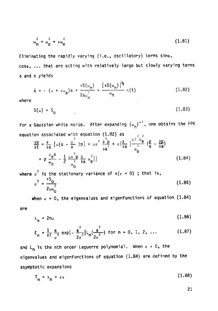
It is convenient to express A in the polar form

A (2.11)

Substituting equation (2.11) into equation (2.10), separating real and

imaginary parts, and replacing Tl with gt, we obtain

, eh eka sinY cosY + gl (2.12)

a° = a — gig ai+ iii cos -

igg sin + (2 13)Y EY aoo zoo Y zoo Y iz ‘

whereE Zn l E Zn

gl = — joa; fo gs1n¢d¢, gz = Ego; fo gcos¢d¢, (2-14)

and

6 = ot - Y . (2.15)

According to this approach, we assume that the gn are small

compared with ho and ko. Next, we determine the mean steady-state

values ao and Yo of the amplitude and phase when gl = gz = 0. They

correspond to a = 0 and Y = 0 and hence they are given by

-·g 6 a + g 26 a3=

gg-sin +

gg-cos (2 16)

Z 1 o 8 wo 2 o Zoo Yo Zoo Yo '

h k3¤ 3 -1. -1 -Boo ao — väo — Zoo cosYo Zoo s1nYo (2.17)

Squaring and adding equations (2.16) and (2.17) yields the frequency-

response equation6 2 2 a 2 2

w 6 +911 zu 6 6 +6av k hQ 2 6 Q 1 2 1• 2 2 2 _Q

- -2 =T

GO - Zlllo GQ + (öl + 4v )Go — 2 lllzÜ

oHence, to the first approximation, the steady-state response is given by

u = aocos(ot - Yo) + ... (2.19)

38

where ao and Yo are given by equations (2.l6)—(2.18).

Next, we determine the effect of the noise (i.e., gl and gz = 0)

on the mean motion. To this end, we let

d = do + dz, Y = YO + Y; (2.2Ü)

Substituting equations (2.20) into equations (2.12) and (2.13) and

linearizing the resulting equations, we obtain

x(t) = Cx(t) + G(t) (2.21)

wherex (t) a (t)

><('¤)={1 }={l ) (2-22)

czG t = , C = 2.23

(2-24)o

-l ä 2 2 -22 3cl — 2 6(6, - 4 woszao), cz —8wO ao - evao ,

-2 92 - 1 _ 1 2 2cz - ao - Bwo ao and ck — 2 e(6, 4 doazao) (2.25)

Ne note that C is a real nonsymmetric matrix.

The general solution of equation (2.21) can be obtained by modal

analysis. The eigenvalues and eigenvectors of C are given by

Cx = xx (2.26)

while the eigenvectors of the adjoint problem are given by

cTv = xv (2.27)

39

Then, the m0daT matrices are

013 012 l l

X X6262 63 63

where

dn = 6263 [6263 + (xn for n = 1 and 2 (2.29)

It is convenient to introduce a transformation that decoupies

equations (2.21). T0 this end, we Tet

x(t) = Xz(t) (2.30)

Substituting equation (2.30) into equation (2.21) and premultipiying by

VT yieids

2[(t) = x3z3(t) + nl (2.31)

22(t) = A2z2(t) + Hz (2.32)

where xn—63nn = 53 + ägE;— g2 for n = l and 2 (2.33)

Then, the statistics of the uncoupied coordinates 23 and 22 are

< zm > = 0 (2.34)

(x t2+x t2) tl t2 —(A 13+x 12)<z,„<t.>z„<r.>>=¤

"‘" ff e

'“" —

0 0

< nm(t2)nn(1'2) > dtldr2 FOT m, I1 = 1, 2 (2.35)

40

where the angle brackets stand for the expectation. As examples, we

consider the cases of sinusoids having nonstationary random amplitudes

and white noise.

2.3.1 Nonstati0nary—Randum—Amplitude Sinusoids

In this case, we let

;(t) = hlcosnt — klsinot (2.36)

where hl and kl are separable nonstationary random functions described

by

hl = fl(Tl)wl kl = f2(Tl)w2 ° (2.37)

Here, the fn are slowly varying deterministic functions of time, whereas

the wn are slowly varying random functions. Road roughness and seismic

ground motion could be modeled by separable nonstationary random

processes. Performing the integrations in equations (2.14) and using

equations (2.33), we can write the nn as

nn(t) = dlnhl(t) — d2nkl(t) for n = 1, 2 (2.38)

whered = —$— [siny + inlii cosy ] (2.39)ln Zw o a cl 00 o

6ln-Cl •

dzn = COSY0 +S'||‘lYO]0o

A narrow—band random excitation is a special case of the excitation

given by equations (2.36) and (2.37). Here, ;(t) is chosen to be a

41

zero-mean Gaussian narrow-band random excitation. It could be obtained

by filtering a white noise through a linear filter [40,140,141]; that

is,

5+:225

+ ßé =BLEQW (2.41)

where 9 is the center frequency of 5 and a is the bandwidth of the

filter. The autocorrelation function of the white noise w is given by

Rw(t) = 2¤SO6(t) (2.42)

where 6 is the Dirac delta function. Substituting equation (2.36) into

equation (2.41) and performing deterministic and stochastic averaging of

the equations describing the modulations of hl and kl with time, one

obtains

hl + é ßhl = JEY2 wl (2.43)

kl + é ßkl = JEY2 W2 (2.44)

The white noise components wl and wzare independent and their auto-

correlation functions are given by equation (2.42). The autocorrelation

functions of hl and kl are

- = -ßlil/2Rhl(t) - Rkl(r) HSOE (2.45)

The correlation time of hl and kl is 0(1/6). This means that for

sufficiently small values of 6, hl and kl are slowly varying functions

of time. Using equations (2.35), (2.38)-(2.40), and (2.45), we obtain

the following stationary statistics of the uncoupled coordinates

TT

Z":(

s (a a +6 a )_ o ln lm 2n 2m 1 1 =<znzm> — lnllm [ln_B/2 + lm_B/2] for n, m 1, 2, (2.46)

42

To the first approximation, the solution of equation (2.1) can be

written as

u = aOcos(0t — Yo) + alcos(0t — Yo) + Yla0sin(ot — Yo) + ... (2.47)

where ao is given by equation (2.18), Yo is given by equation (2.17),

and the statistics of al and Yi are

< al > = 0, < Y! > = 0 (2.48)

(2.49)

2 2 2 22 °1()1°C1) 2 ¤2(Ä2_c1) 2 2°1“2(Ä1'C1)(Ä2'c1)‘Y1> = -*2*- QR +

-

<Z2> + -2* ‘ZIZ2>c c c22

22 2 (2.50)

¤l(Ä1_Cl) 2 ¤2(Ä2_C1) 2“1°2

<Z2’ + *- (M + M * 2C1)<ZlZ2>C2 C2 C2

(2.51)

Using equations (2.20) and (2.48)—(2.51), we obtain the following

statistics for the amplitude and phase of the response:

< a > = ao, og = oäl (2.52)

< Y > = Yo, ci = oil (2.53)

2.3.2 White Noise

In this case, we have

RE(1) = 2¤SO6(r) (2.54)

43

The autocorrelation function given by equation (2.54) implies that 5 is

a fast varying random function of time. Terms including 5(t) in

equations (2.12) and (2.13) can be replaced by their means and

fluctuating components. This stochastic averaging is restricted to

random excitations with small correlation time compared with the

relaxation time of the oscillator. The main advantage of stochastic

averaging is to decouple the amplitude and phase equations (2.12) and

(2.13). However, the presence of the deterministic excitation will keep

this coupling. It is applicable to any low—intensity random excitation.

Using equations (2.14), (2.33)-(2.35), and (2.54), we can express

the expected values and the mean-square values of the uncoupled

coordinates zn as

<zn> = 0 (2.55)

2

<znzm> [1 + Einläéäéimliil] for n,m = 1,2 (2.56)

o n m o 3

2.4 Second-Order Closure Method

The mean motion given by equations (2.16)—(2.18) has no feedback

from the perturbations due to the noise. This limits the applicability

of the linearization method in the transition zone separating stable and

unstable periodic responses. In fact, the preceding linearization

scheme predicts infinite mean-square responses at the bifurcation points

separating stable from unstable mean responses. To overcome this

problem, we propose a second-order closure method. To describe the

44

method, we find it convenient to express A in equation (2.10) in the

form

1 ivTIA = ä (x — iz)e (2.57)

Substituting equation (2.57) into equation (2.10), separating reai and

imaginary parts, and repiacing T1 with et yieids

_ ek Zn/wX = - % EÖEX · €\)€Z + ·· ä fo

0eh

Zn/w2 = — é 6602 + 60Ex + ägä + ä; fo O gcosnt dt (2.59)

where

ae = - 61 + ä + Z2) (2.60)

6a = 6 - (X2 + Z2) (2.61)

Next, we separate each of x and 2 into mean components x0 and 20 and

random components yl and y2 according to

x = xo + yl and 2 = 2O + y2 (2.62)

Substituting equations (2.62) into equations (2.58)-(2.61) and

separating mean and fiuctuating components, we have

45

mggn motion

. _ 1 1 2 3 1 2 2 3 2 3 3X0 ‘* EÖIXO · '§ EUJOÖZXO · ä' ECDOÖZXOZO • EVZO XOZO Zo

3 2 3 2 1 2 9 2 3‘ [Ö [5 Xo

1 2 ]< > 1 ~ 3: < 3> < 2> 3€°< 2 > < 3>

y1 + y1y2 ) +g1g ( y1y2 + y2 ) +;E

(2.63)

. — -1 1 2 2 1 2 3 3 220 - 2 26120 - 8 00061x020 - 8 2006120 + 00x0 - 80 x0 - 80 x020

o o

9 1 2 2 3 3 2 2- [gi? x0x02

3 1 2 2 3— lä 5 ¤<¤O62(<¥3¥2> + <>'2>)

sh(2-64)

fiuctuating motion

. n1>j(t) = Cy(t) + @(4:) + 4j(y„y2)„ [4 = {,12} (2-65)

Zn/wo 0 Zn/w0g1(t) = - äg f gsinnt dt, g2(t) = gg f gcosot dt (2.66)

o o

- L 3. 2 2 L 2 2 ksC1 ‘2 E61 " 8 EMOÖZXO · 8 EMOÖZZO + 40,0 XGZO46

1 2 3 2 9 2cz = - E ewoözxozo - ev xo 20 (2.68)

- L4 swoszxozo + 2V - Sw xo - 8m 20 (2.69)0 O

1 1 2 2 3 2 2 3C11 = ä' 661- 6wO61XO — ä' XOZO (2.70)

1 2_ 2 2T11 = - ä-3

3 2 2+ 2ZO(Y1Y; · <Y1Y2>) + y1 ·<Y1>3

3 2 2· <Y1Y2>) + Y; · <Y2> + Y1Y2 · <Y1.Y2>] (2•7l)

nz2

2 2 2 3 3+ 3ZO(Yz — <Y2>) + ylyz — <y1yg> + yz — <Y2>]

2 2 2 2- $:1-2 [3><O(y1 — <Y1>) + ><O(yz - <Yz>) + 2ZO(Y1yz

O

3 3 2 2— <y1yz>) + Y1 - <y1> + y1yz — <y1yz>] (2-72)

47

For noise whose intensity is small compared with ho and kO,

y1 and y2 are small compared with xo and 20, and hence central moments

higher than the second can be neglected in equations (2.63)-(2.65).

Consequently, it follows from equations (2.63) and (2.64) that the

steady—state mean motion is given by

%661XO - EWÄÖZXÄ - é - EVZO + + zg

3 Z 3 2 1 2 9 Z 3· hf woözxo lo Ewoöäxo Xo

1 2 Eko· E

6wO62ZOI<_y1_y2> +E

= Ü (2.73)

1 1 2 2 1 2 2 3 2 3 2ä- 66120 6wO62XoZO 6:.106220 + 6vXO XO XOZ0

9 1 2 2 3 3 2 2— [ggü xo + ä oao62z0]<y1> - [gi; xo + ä oaO62zO]<y2>

6h- [ä 0 (2.74)

Ne neglect central moments beyond the second, and hence neglect N in

equations (2.65). Using modal analysis to decouple these equations, we

find that the statistics of the uncoupled coordinates 21 and 22 for a

narrow-band random excitation are given by equations (2.34) and (2.46)

where

6(Xn-C1)Edln = *2.;* d2n = · Q (M5)

48

For the case of a white noise, these statistics are given by equations

(2.55) and (2.56). The mean—square values of yl and y2 have the form

described in equations (2.48)—(2.51) for al and vl.

To the first approximation, the solution of equation (2.1) can be

expressed as

u = (xo + yl)c0snt + (20 + y2)sinnt + ... (2.76)

Equations (2.48)—(2.51), (2.73) and (2.74) and either equations

(2.46) or equations (2.56) represent a system of five simultaneous

nonlinear algebraic equations. A modified Powell‘s hybrid algorithm is

used to solve this system.

For the case of a narrow-band random excitation, premultiplying

equations (2.65), (2.43) and (2.44) by yl, y2, hl and kl and taking the

expectations of the resulting equations, we have

P = BP + Q (2.77)

wherez z T

g:andB and Q are given in Appendix I. The stability of a particular

fixed point of equations (2.73), (2.74) and (2.77) to a perturbation

proportional to exp(xt) depends on the eigenvalues of C and B.

49

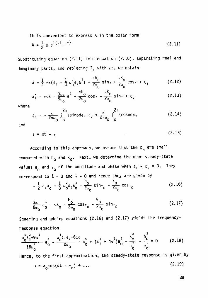
2.5 Semi—Linearization Method

Rajan and Davies [141] developed a method for the determination of

the response of single—degree-of—freedom systems to zero—mean narrow-

band random excitations. In this section, we generalize this method for

the case of nonzero-mean random excitations and point out its

limitations.

To determine the stationary mean-square value<x2

+z2>

of the

amplitude, we follow Rajan and Davies and assume average values for

se and ve. Substituting equation (2.36) into the integrands in

equations (2.58) and (2.59) and performing the deterministic averaging,

we find that the integral terms in equations (2.58) and (2.59) become

akl/Zoo and ehl/Zoo, respectively. Then, we combine equations (2.58)

and (2.59) into

d<x2+z2> _ 2 2 l > 2 79—T———Öe<X+Z>+F<Zh+Xk (•)

whereO

h = ho + hl and k = ko + kl (2.80)

Next, we add k times equation (2.58) to h times equation (2.59), use

equations (2.43) and (2.44), and obtain

äfäggäää = v€<xh — zk> - é (se + 6)<zh xk>

2 2

xg <zwl + xw2>

(2,81)Subtractingk times equation (2.59) from h times equation (2.58) and

using equations (2.43) and (2.44), we obtain

50

gjääigßi = - 6e<zh + xk>zk>+

7% <xwl — zN:> (2.82)

Taking the expected values of equations (2.58) and (2.59) yields

ckgä%Z = —é e5€<X> - 66€<z> + E39 (2.83)

0eh

<z> (2.84)0

Following Rajan and Davies, we assume that <xwi> = O and <zwi> =

0. Then, the stationary solutions (l0ng—time averaging) of equations

(2.79) and (2.8l)—(2.84) are given by

2(6 +6)6FZ 462

wO6€[46e(6e+6) ] 6e+46e e

where

Fg = ä (hä + kg) and <F2> = Fg + ä <hi + ki> (2.86)

A sh0rt—time averaging is implied in equation (2.86). Equation (2.85)

is a nonlinear algebraic equation in<x2

+z2>.

The response is assumed

to be psuedo sinusoidal and the frequency shift and damping parameters

of the system are given by

6 = - 6 + lw26 <x2

+z2> (2 87)

e 1 4 o 2 '

6e = 6 - ää— <x2 + z2> (2.88)0

51

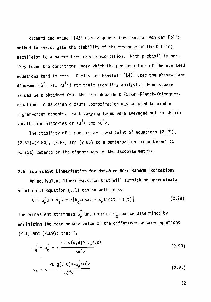
Richard and Anand [142] used a generalized form of Van der Pol's

method to investigate the stability of the response of the Duffing _

oscillator to a narrow—band random excitation. with probability one,

they found the conditions under which the perturbations of the averaged

equations tend to zero. Davies and Nandlall [143] used the phase-plane

diagram [<u2> vs. <u2>] for their stability analysis. Mean—square

values were obtained from the time dependent Fokker-Planck-Kolmogorov

equation. A Gaussian closure „pproximation was adopted to handle

higher—order moments. Fast varying terms were averaged out to obtain

smooth time histories of <u2> and <u2>.

The stability of a particular fixed point of equations (2.79),

(2.81)—(2.84), (2.87) and (2.88) to a perturbation proportional to

exp(xt) depends on the eigenvalues of the Jacobian matrix.

2.6 Equivalent Linearization for Non-Zero Mean Random Excitations

An equivalent linear equation that will furnish an approximate

solution of equation (1.1) can be written as

u + uäu + deu = 6[hOcos0t - kosinnt + g(t)] (2.89)

The equivalent stiffness wi and damping He can be determined by

minimizing the mean-square value of the difference between equations

(2.1) and (2.89); that is

<u u u >- <uu>(1);: (1);)+ (2.90)

<u g(u,u)>-u;<uu>ue = 6 (2.91)

52

where

(2.92)

Next, we separate u into a mean component uo and a random component ul

according to‘

u = uo + 0, (2.93)

where

0; + 0;uO + U;00 = 6[h;cosot - kosinot] (2.94)

01 + U;ul + U;0, = 6;(t) (2.95)

Substituting equation (2.92) into equations (2.90) and (2.91) and using

equation (2.93) yieids

0; = 0; + [0; + <ui>]”1[6au; + 66au;<ui> + 6a<u:>] (2.96)

U; = - 66, + [0; + <0i>]’1[ ä 66,0; + 2e6,0;<0i> + ä €62<0:>] (2.97)

Using equation (2.94), we obtain

U; U; = QZU; (2.98)

U; = ä D“(h; + 2n;k; + k;), U; = 0“U; (2.99)where

0 = [(U; -62); + (2.100)

53

A short-time averaging is implied in equations (2.98) and (2.99). For a

Gaussian response <u:> =3<ui>2

and for a psuedo sinusoidal response

when 5 is a narrow—band random excitation, the complex frequency

response function H(u) can be obtained by combining equations (2.95) and

(2.41); that is,

e8%QH(w) = ——;——;—-—————;;—T;———- (2.101)

(we-w +lueu)(Q -w +l8w)

The mean-square values of u, and ul can be written as

= (2-102)uewe[(0 —we) +(uE+B)(uE0 +Bwe)]

_2 e2¤SOQ2(u€+B)‘“1> = (2*03)¤e[(¤ —we) +(uE+6)(ueo +6ue)]

For the case of a white noise, we have2 S 2 SE TT

€ll'

<ui> = —-?9 , <Qi> = --2- (2_104)

uewe ué

2.7 Numerical Results

In the pv—plane, where p the frequency—response equation

(2.18) provides a one-parameter family of response curves. when ¤ = 0,

the response curves are symmetric with respect to the p-axis. Let fg =

(hä + kä)%. when fo = 0, the curves of the family degenerate into the

line p = 0 and the point v = 0 and p = 1. As fo increases, the curves

first consist of two branches — a branch running near the V-axis and a

branch consisting of an oval, which can be approximated by an ellipse

54

having its center at (0,1). As fo increases, the ovals expand and the

branch near the »—axis moves away from this axis. when fä reaches the

critical value 16/2762(6 = 6l = 62), the two branches coalesce, and the

resultant curve has a double point at (0, ä) as shown in Figure 2.1. As

fo increases further, the response curves become open curves, which

continue to be multi—valued functions until fg exceeds the second

critical value 32/275;. Beyond this critical value, the response curves

are single-valued functions for all values of v.

when 6 ¢ 0, the response curves lose their symmetry with respect to

the 6 axis and bend to the right for a > 0 (hardening nonlinearity) and

bend to the left for 6 < 0 (softening nonlinearity). Representative

curves are shown in Figure 2.2 when a > 0. when fo = 0, the family of

curves degenerates into the line 6 = 0 and the point 6 = 1 and v =

3a/Zwg. As fo increases, the response curves consist of two branches -

a branch running near the p axis and a branch consisting of an oval. As

fo increases further, the oval expands and the branch near the o-axis

moves away from it. when fo reaches a critical value fol, the two

branches coalesce and have a double point. As fo increases beyond

fol, the corresponding response curve continues to be a multi-valued

function of o until a second critical value fo2 is exceeded. For all

values of fo greater than fo2, the response curve is a single-valued

function of u.

Not all of the solutions given by the frequency-response equation

(2.18) are realizable because some of them are unstable. The solution

given by the frequency-response equation (2.18) is stable if none of the

55

eigenvalues defined in equation (2.26) has a positive real part. The

eigenvalues are given by the characteristic equation

A2- c6(l - 26)) +

EZA= 0 (2.105)

where 2 2A = ä Sql - 46 + 262) + vz _ 6%+% and A =%„„;a; (2.106)

“o wo

when A < 0, the roots of equation (2.105) are real and have different

signs. Hence, the predicted mean motions correspond to saddle points

and are unstable. These correspond to the interior points of the

ellipse A = 0 in the 6-0 plane. Since the discriminant of equation

(2.105) is

2 2 224vapD=5p

-4\Jperiodicmotions corresponding to D < 0 are focal points, while those

corresponding to D > 0 are nodal points. For 6 > 0, these points are

stable or unstable depending on whether p is greater or less than é.

The dark lines in Figures 2.1 and 2.2 separate stable from unstable

solutions; all solutions corresponding to points above the dark lines

are stable and those corresponding to points below the dark lines are

unstable.

Figure 2.3 shows that the mean response predicted by the

perturbation expansion is in good agreement with that obtained by

numerically integrating equation (2.1) using a fifth—order Runge—Kutta

Verner technique (numerical simulation).

56

The effect of the excitation frequency on the primary mean response

is shown in Figure 2.4. The linearization method is used in Figure 2.4a

to predict the effect of a narrow-band random excitation on the mean

response. Near a saddle-node bifurcation point (the fixed point loses

its stability with a real eigenvalue crossing the imaginary axis) and

Hopf bifurcation point (the fixed point of the mean motion loses its

stability with the real part of a complex conjugate pair of eigenvalues

changing sign from negative to positive), the mean motion is sensitive

to any outside perturbations and the linearization method fails. In

Figure 2.4b, the second-order closure method is used to obtain the mean-

square response. The second-order closure method provides the necessary

feedback from the pertubations caused by the noise to the mean motion.

This limits the second-order moments predicted by the linearization

method at the bifurcation points separating stable from unstable mean

responses. Since a > 0, the response curves in Figure 2.4 are bent to

the right, causing multi—valued regions. The multi-valuedness is

responsible for a jump phenomenon at the saddle-node bifurcation points

that leads to an abrupt change in the response.

The semi-linearization method is based on assuming an average value

<x2+

z2>of the amplitude. With this assumption, substituting

equations (2.62) into equations (2.58)-(2.61) and separating mean and

fluctuating components for the case of a narrow-band random excitation,

we have

57

mean motion

. _1 1 2 2 1 2 2 3 2XO 6wO62XO 6wO62XOZO - EVZO XOZ0

Lsg 3 L 2 Lsg 2 1 2T 600 20 ‘ [6 600 [6 Emoözxo

36a 2 EkO— gg; ZO1<Y2> + ägg (2.108)

. _ 1 1 2 2 1 z 2 308 2ZO —

2 66120 —8 EMOÖZXOZO —

8 6606220 + EVXO XO

L2 2 E L 2 2” 860 Xozo [860 xo + 8 Emoö2Zo[<y1>

kg L 2 2 220— [8wO xo + 8 66062zO]<y0> + 8;; (2.109)

fTuctuating motion

· 1 l 2 2 l 2 2 36a 2y = [— 6 -

— 6 x -— 6 z ly + [- + ———

1 2 E 1 8 Emo 2 o 8 gmo 2 o 1 Ev 860 Xo

36a 2€k[

+ 8wO zolyz + Zwo (2.110)

· - Lsg 2 Lsg 2 L .L 2 2y2 — [EV —

8wO XO —8wo zolyl + [2 661 - 8 6wo62XO

1 2 2 Ehx- E 06060zO]y0 + EE; (2.111)

The mean motion given by equations (2.108) and (2.109) provides a

feedback from the noise through <yi> and <y;>. However, the cross

corre1ation <y1y2> has no contribution and the coefficients of the

terms xo<yi> and zO<y;> are one—third of those given by equations (2.63)

and (2.64) obtained by the second-order closure method. The

Tinearization method and the second-order closure method have the same

form with respect to the fTuctuating motion. According to equations

58

(2.65), the fluctuating motion given by equations (2.110) and (2.111)

does not include the xozo terms. The coefficients of xäyl and

zäyz are one-third those given by equations (2.65). As a result, the

accuracy of the semi—linearization method is somewhere between the

linearization method and the second-order closure method. Figure 2.5

shows a comparison among the results of these three methods and that

obtained by the method of equivalent linearization. Away from the

transition zone between stable and unstable responses, the results are

in good agreement. The linearization method is simple and direct but it

fails to give good approximations to the mean—square response at the

stability boundaries. The second-order closure method is expected to be

the most accurate but it requires the solution of a system of five

simultaneous nonlinear algebraic equations.

The local stability of the stationary mean and mean-square response

is analyzed. Figure 2.6 shows the effect of a low intensity noise,

around the natural frequency oo of the system, on the stability of the

mean response. The strength of the noise is taken as 1/450 of the

strength of the deterministic excitation. Since a = 0, the response

curve is symmetric with respect to the <u2> - axis. The response curve

has its peak at the perfectly—tuned frequency n = we (i.e., v = 0). The

mean motion loses stability when lvl 2 0.093. The presence of the noise

expands the stability region lvl 2 0.1.

As the amplitude of the mean excitation increases, the effect of

the noise on the steady—state mean response decreases as shown in Figure

2.7.

59

2.8 Conclusions

A second—order closure method is presented for determining the

response of nonlinear systems to random excitations. As an example, the

method is used to determine the response of the Duffing-Rayleigh

oscillator to an excitation consisting of the sum of a deterministic

harmonic component and a random component. The random component is

assumed to be white noise or sinusoidal whose amplitude and phase have

two parts - a constant mean and a separable nonstationary random

process. The method of multiple scales is used to determine the

modulation of the amplitude and phase with the nonlinearity and the

excitation. Three methods have been used to determine the mean and

mean-square responses from the modulation equations. The local

stability of the stationary mean and mean-square responses is

analyzed. For some range of parameters, the presence of noise can

expand the stability region of the mean response. Comparisons of the

results of these methods with the results obtained by using the method

of equivalent linearization are presented.

The present analysis attacks the problem in a way that the

statistics of the response can be determined for general types of

excitation and nonlinearity. The nonlinearity bends the frequency-

response curves, causing multi-valued regions in the mean-square

response. The multi-valuedness is responsible for a jump phenomenon.

60

CHAPTER 3

A GENERALIZED METHOD OF EOUIVALENT LINEARIZATION

The application of the method of equivalent linearization for

solving nonlinear vibration problems is reviewed. The conceptual

drawbacks and limitations of this method are discussed. A

generalization of the method of equivalent linearization is presented.

The method is based on replacing the nonlinear governing equation by two

equivalent linear equations. This generalization scheme overcomes some

of the drawbacks and limitations and also contributes to a better

understanding of the basic phenomena introduced by the presence of

nonlinearities. It provides some means to describe the non—Gaussian

feature of the response of a nonlinear system. An attempt to explain

some experimental phenomena in the large—amplitude response of aircraft

panels to an acoustic excitation is presented. These include broadening

effects and a shift in the resonant frequency. The proposed approach is

illustrated by investigating the response of a class of nonlinear

systems to random excitations. The effect of the system parameters on

the response is analyzed for the cases of a Gaussian white noise and a

superharmonic narrow—band random excitation of order-three.

3.1 Introduction

Over the years, a number of approximate methods for solving

nonlinear stochastic problems has been developed and recently emphasis

has been placed on their adoption for computers. These include the

61

method of equivalent or stochastic linearization, perturbation methods,

functional series representations, and digital- and analog—computer

simulations. However, the method of equivalent linearization has the

widest range of applicability. This method is potentially useful for

systems having nonlinear damping, nonlinear restoring forces,

nonlinearity of a mixed type, and nonlinear hereditary forces, and it

can be easily extended to the case of multi-degree-of-freedom systems.

The method of equivalent linearization was first proposed by

Jacobsen [144]; it is based on the method of averaging of Krylov and

Bogoliubov [76] for deterministic nonlinear problems. Booton [77] and

Caughey [78,47] introduced independently this method to statistical

problems.

To describe the method, we consider

x + mäx + eh(X,i) = F(t) (3.1)

which describes the response of a single-degree—of-freedom (SDOF) system

to a random excitation. Here, ou is the linear natural frequency,

h(x,x) is a nonlinear force, 6 is a small but finite constant, and F(t)

is a zero—mean random excitation. According to the method of equivalent

linearization, equation (3.1) is replaced with the linear equation

x + wéx + 26uex = F(t) (3.2)

where the equivalent stiffness wg and damping ue parameters are

determined by minimizing the mean—square value of the difference between

equations (3.1) and (3.2); that is,

62

Q.; = w; + E %%;i)i (3.3ä)

ue = £ih$§L&lZ (3.3b)2<x >

where the angle brackets stand for the expectation and the response x is

assumed to be stationary. A knowledge of the probability-density

function p(x, x; tlxo, xog to) is needed to find the expectations in

equations (3.3). If available, one can use the stationary probability—

density function of the original nonlinear equation (3.1). As an

approximation, one can use the probability—density function of the

equivalent linear equation (3.2).

Iwan and Gates [145] investigated the accuracy of the various

available techniques in approximating the equivalent linear system

parameters. They considered the response of a nonlinear hysteretic SDOF

osciliator to an earthquake excitation. Iwan and Patula [146] concluded

that the mean-square error minimization is at least as good as any other

type. It can be shown that the mean-square error minimization ensures

the same <x> for both the nonlinear and equivalent linear systems and

the difference in<x2>

for both systems is a minimum.

when the input is Gaussian and G(x,x) satisfies certain smoothness

conditions, the equivalent stiffness and damping parameters can be

written as [79,80]

„„; = < > (3.4a)

zw; = < > (3.4b)ax

63

where

g(x,x) = aäx + ;h(x,x) (3.5)

Z .

If the matrix [EEX;gif;] is not singular, equations (3.4) will yield a

true minimum solution [82]. According to equations (3.4), even

nonlinearities contribute nothing to the equivalent linear system

parameters. This means that the applicability of the method of

equivalent linearization is limited to odd nonlinearities.

when the input is Gaussian, the method of equivalent linearization

predicts a Gaussian response, whereas the original nonlinear equation

(3.1) may predict a non-Gaussian response. To describe the non-Gaussian

feature of the response, Beaman and Hedrick [147] and Crandall [148]

represented the probability—density function p(x) by a truncated Gram-

Charlier expansion. The first term in the expansion is Gaussian and it

is identical to the one obtained by using the method of equivalent

linearization.

Kazakov [81] generalized the method of equivalent linearization to

multi-degree-of—freedom nonlinear systems. Spanos and Iwan [82]

considered the existence and uniqueness of solutions generated by the

method of equivalent linearization. Iwan and Mason [80] used the same

technique for systems subject to nonstationary random excitations.

For systems with hysteresis, Caughey [149] applied a modified

version of the equivalent-linearization procedure. The response is

64

assumed to be sinusoidal with sTowTy varying amplitude and phase

(narrow—band process). Hence,

x = a cos(6Ot + 6) and x = — moa sin(mOt + 6) (3.6)

Using the method of variation of parameters and eTiminating fastly

varying terms, we obtain

2 2+ , <*¤<¤>> (3 7+w =w ———· .6E O r <a—>

<hZ(a)>ue = -

——————;- (3.7b)Zum <a >

o

where

2TT

h1(a) = f a h(a cos¢, - moa sin¢)cos¢d¢ (3.8a)oZT!

h2(a) = f a h(a cosa, — moa sin¢)sin¢d¢ (3.8b)o

and ¢ = mot + 6 (3.8c)

However, the Toss of energy is reTativeTy Targe for hysteretic

systems. This broadens the frequency content of the response and

eTiminates its narrow-band nature. As a resuTt, the accuracy of the

method of equivaTent Tinearization is rather poor for inelastic

structures and seriousTy overestimates the energy dissipation in such

systems [150]. Monte—CarTo-simuTation resuTts of the response of

bilinear hysteretic systems to a Gaussian white noise indicate that the

accuracy of the method of equivaTent Tinearization deteriorates as the

65

damping increases and the response probability-density function is

significantly non—Gaussian [65]. The proposed method in Section 3.3

improves the accuracy of the solution by accounting for some of the

wide-band character of the response.

Many authors [85-89] used the method of equivalent linearization to

determine the response statistics of hysteretic degrading systems. A

generalization of the method of Atalik and Utku to the case of nonzero-

mean problems is proposed by Baber and wen [85].

For large-amplitude responses, the method of equivalent

linearization fails to give a decent approximation to the response. It

does not account for all interactions between the nonlinearity and the

excitation. The nonlinearity creates a whole range of interesting

phenomena in the response of structures to deterministic and random

excitations. These include non—Gaussian responses, multi-valued

responses, jumps, modal frequency shifts, broadening effects, and

superharmonic, subharmonic, ultrasubharmonic, and combination

resonances. The equivalent linear model equation (3.2) fails to account

for most of these phenomena. This limits the applicability of the

method of equivalent linearization to weak nonlinearities and soft (very

small) excitations [151,51].

A number of experimental studies tested the applicability of the

method of equivalent linearization. They include the studies of

Nikiforuk and west [90], Smith [91], Gelb and Van der Velde [93], and

Morton [92]. Bulsara et al. [83] made a comparison between the results

of an analog—computer simulation and those obtained by the method of

66

equivalent linearization for the Duffing oscillator. The results show

that the method of equivalent linearization underestimates the low-

frequency part and overestimates the peak height of the spectral

density. when h(x,x) = ax} orßxzx

and F(t) is a Gaussian white noise,

the percent error in the mean-square response obtained by using the

method of equivalent linearization is about 15% [79}. The method of

equivalent linearization underestimates the root-mean-square response of

a nearly elasto-plastic system by up to 50-60 percent [150].

Many authors [152-158] investigated the sonic fatigue design of

aircraft strucutres based on a linear or a nonlinear analysis. The

linear structural theory predicts larger mean—square responses and

smaller modal frequencies than the corresponding experimental results.

This leads to a poor estimate of the service life of strucutral

elements. Mei and Prasad [155] investigated the effect of nonlinaer

damping on the random response of beams to acoustic excitation. The

excitation was taken to be a white noise. Test results show an increase

in the resonant frequency, a broadening of the frequency-response

curves, and a shift in the response peak. Assuming that the beams allow

large deflections and the fundamental frequency is predominant leads to

a modal equation of the Duffing type. The method of equivalent

linearization can only account for a nonlinear shift in the frequency of

the Duffing oscillator. Mei and Prasad [155] considered the influence

of the two nonlinear terms

alxxz + azxzx (3.9)

67

on the broadening of the response; the first term is a nonlinear damping

term, whereas the second terms is a nonlinear inertia term. The

experimental results of Smith et al. [156] suggest the presence of the

nonlinear damping term in the model of a simple clamped panel. The

proposed method explains some of the broadening behavior without

introducing nonlinear damping models.

In Section 3.3, a generalized method of equivalent linearization is

presented. It provides some means for describing the non—Gaussian

feature of the response and preserving some of its wide-band

character. The nonlinear governing equation of motion is replaced by

two equivalent equations: one is linear and the other is nonlinear.

According to the method of equivalent linearization, the latter is

replaced by an approximate linear equation. The interaction and

feedback between the nonlinearity and the excitation creates nonlinear

resonances. These lead to a linear shift in the natural frequency and

an adjustment in the strength of the primary excitation. The latter

contributes to the broadening effects. The proposed method is

illustrated by investigating the response of the Duffing and Van der

Pol-Rayleigh oscillators to random excitations. To test the soundness

of the method, we compare the mean—square responses obtained by using

the proposed scheme with those obtained by using the Fokker-Planck-

Kolmogorov equation.

68

3.2 Limitations of the Method of Equivalent Linearization

0ne of the major limitations of the method of equivalent

linearization is that the response of a system to a deterministic

excitation occurs at the driving frequencies with no contribution from

other harmonics. As an example, we consider the response of the Duffing

oscillator to a deterministic harmonic excitation. The problem is

governed by

x + wäx + Zgtx + tax} = G cosot (3.10)

The linearized version of the Duffing equation (3.10) has the form

3 + w;X + Zepi = G cosot (3.11)

The steady-state solution of equation (3.11) can be written as

x = A cos(ot — ;) (3.12)

whereG -1 2

^ = ¢‘TV"—ü · 1 = tan ljzislzl (3-13)[(we-Q ) +(2epQ) I w€—Q

and

ug; = (nä +

gqdzNext,we consider different resonances and compare the dynamic responses

obtained by using the method of averaging and the method of equivalent

linearization with those obtained by numerically integrating equation

(3.10) using a fifth-order Runge—Kutta Verner technique (numerical

simulation).

69

3.2.1 Primary Resonance

In this case, we let

9 = wo + ev, and G = eG (3.15)

Using the method of averaging [95,96], one can write the steady—state

solution of equation (3.10) as

x = aOcos(0t - yo) + ... (3.16)

where „

- ,130 + sinyo = 0 (3.17)o

olao - gg- aag + gg- cosyo = 0 ‘ (3.18)o 'o

Comparing equations (3.16)—(3.18) with equations (3.12)—(3.14), we

conclude that the solution obtained by using the the method of

equivalent linearization has the same Frequency content as that obtained

by using the method of averaging. Figure 3.1 shows that the responses

predicted by using the method of averaging and the method of equivalent

linearization are in good agreement with that obtained by using

numerical simulation.

3.2.2 Superharmonic Resonance of Order-Three

In this case, we let

39 = mo + cvz (3.19)

70

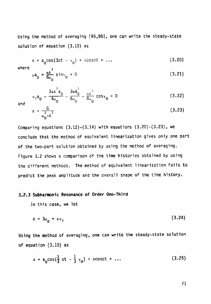
Using the method of averaging [95,96], one can write the steady-state

solution of equation (3.10) as

x = aocos(3ot — yo) + ncosot + ... (3.20)

where 3nao +

äSanyo = 0 (3.21)

3Aza

3ai ‘

¤ oa >COSYO = O (3.22)

and °O 0

GA = -j-g (3.23)

wO—Q

Comparing equations (3.12)—(3.14) with equations (3.20)-(3.23), we

conclude that the method of equivalent linearization gives only one part

of the two—part solution obtained by using the method of averaging.

Figure 3.2 shows a comparison of the time histories obtained by using

the different methods. The method of equivalent linearization fails to

predict the peak amplitude and the overall shape of the time history.

3.2.3 Subharmonic Resonance of Order One-Third

In this case, we let

Q = 3wo + ev3 (3.24)

Using the method of averaging, one can write the steady-state solution

of equation (3.10) as

x = a cos(l Qt - l ) + Acosot + (3 25)O 3

••• •

71

where

pa + Ejäéä siny = 0 (3 26)0 8oO o '

9aaOA2 Qaag Qaagnvado - - · COSYO = Ü (3.27)

o o 0

Comparing equations (3.12)-(3.14) with equations (3.25)—(3.27), we

conclude that the method of equivalent linearization fails to give the

whole frequency content obtained by using the method of averaging as

shown in Figure 3.3.

The above analysis shows that the method of equivalent

linearization fails to account for nonlinear resonances.

3.3 Proposed Method

The present work is concerned with the response of single-degree-

of-freedom systems to random excitations governed by the equation

x + oäx + 2px + k(x,x) = F(t) (3.28)

where k is a nonlinear function of x and x. The excitation F

represents a stationary random excitation with a zero mean and a

Gaussian probability-density function. The main idea underlying the

proposed method is to divide the excitation into two parts as F =

fl + fz. The first part fl has a spectral density around

oo, whereas the second part fz has a spectral density away from oo.

Moreover, the solution of equation (3.28) is expressed as

72

Ix= U + V (3.29)

where

u + wäu + 2pu = f,(t) (3.30)

The solution of equation (3.30) can be written in terms of Duhamel's

integral; that is,

u(t) = f hl(:)f,(t — :)dz (3.31)o

where

(3.32)

Since fz has no spectral component around wo, the solution given by

equation (3.31) has no irregularities. It follows from equation (3.30)

that the output spectral density of u is

sf (M)2$„(·¤) = (3-33)

(wO—w ) +4u w

Substituting equation (3.29) into equation (3.28) and using

equation (3.30), we obtain the following equation governing v:

v + wäv + Zuv + k1(u,ü,v,v) = f1(t) - k(u,u) (3.34)

wherek1(u,u,v,v) = k(u + v, u + v) - k(u,ü) (3.35)

The nonlinear function k adjusts the external excitation by k(u,u) and

leads to parametric excitations and shifts in the linear stiffness and

73

damping parameters through kl. Next, we replace equation (3.34) with

the equivalent linear equation

v + oäv + Zuev = r(t) (3.36)

w=u>+—+,2; =2u+——·r (3.37)E

Oand

r = fl - k(u,u) (3.38)

The term k(u,u) in the excitation r accounts for part of the non-

Gaussian feature of the nonlinear response x. Because the method of

equivalent linearization cannot account for parametric excitations, we

neglect the parametric terms in equations (3.36)-(3.38). we note

that Bruckner and Lin [161] used the method of equivalent linearization

to replace the original Ito equations with linear Ito equations under

certain optimal conditions for parametric excitations. The solution of

equation (3.36) can be written in terms of Duhamel's integral as

v u(: (3.39)0 0

where

h2(t) = (wg -

ué)_%

EE

Slh(w; -u;)%t (3.40)

3.4. Examples and Accuracy

3.4.1. The Duffing Oscillator

In this case, we have

k(x,x) =¤x3 (3.41)

74

The equivalent stiffness and damping parameters and the excitation for

equation (3.36) can be written as

2 2 1 2 3 u 2de = wo + <3au v + 3auv + av > / <v > (3.42)

ue = u (3.43)

r = fl — au? (3.44)

The presence of aua in the excitation r provides some of the non-

Gaussian feature of the nonlinear response x. The term <u2v2> accounts

for both an increase in the linear natural frequency and ultra-

subharmonic resonances, the term <uv3> accounts for the subharmonic

resonance of order 0ne—third, and the termu3

in r accounts for the

superharmonic and combination resonances. Neglecting the subharmonic

and ultrasubharmonic resonances, we rewrite equation (3.42) as

dä = ug + 3a<u2> + / <v2> (3.45)

If we assume that v is Gaussian, then <v“> =3<v2>2

and equation (3.45)

becomes

mz=

bz+ 3a[<u2> + <v2>l (3.46)

e o

Identical results could be obtained by using the method of averaging

(details in Appendix II). A nonlinear algebraic equation in <v2> for

the equivalent linear equation (3.36) can be written as

75

2 Q Sfl(w) 2 Q Su3(w)<V>=Iv?—1d~»+¤I¢—2Tw··rd¤·

·"¤ (u)e·u.l ) +4).1 CL) "¤ ((1|e·(u ) +4].1 ul

— 2¤·I I I I I h,(T,)h,<T,)h,(T,)h,(T.)h,(T,) < f,<t — T,)0 0 0 0 0

f2(t - T2 - T3)f2(t - rg - r„)f2(t - tz - 15) > dtldtzdtgdrgdts (3.47)

Using equation (3.29), we can express the mean-square response as

2 2 ;<x > = <U > + <V > + 2<UV> (3_43)

where <v2> is given by equation (3.47) and

<uv> = — a I h2(T)<u(t)u3(t — T)>dT (3.49)0

Substituting equation (3.31) into equation (3.49), we obtain

<¤V> = — ¤I I I I I h2(T)h,(T,)h,(T2)h,(T,)h,(T,)0 0 0 0 0

< f2(t - t1)f2(t - 1 — T2)f2(t - T — T3)f2(t - t — r“)dtdrldt2dt3dt“(3.50)

The probability—density functions of fl and fz are needed to

perform the integrations in equations (3.47) and (3.50). In the present

work fl and fz are assumed to be Gaussian functions. Using the Gaussian

moment relations, we find that the third integral in equation (3.47)

vanishes and hence

2E Q

SU3(u) = 9<u >2SU(w) + 6 II‘°’‘°° (3.51)

76

and

<uv> = — 3a<u2> f h2(z)RU(r)dr (3.52)o

or

<UV> (t + rl — r2)drdr1dr2O

° °2 (3.53)

A Superharmonic Narrow—Band Random Excitation

Raghunandan and Anand [159,160] considered the problems of

superharmonic resonance of order three and subharmonic resonance of

order one-third in stretched strings. They started by assuming

solutions similar to those obtained by using the method of averaging,

that is;

x = u + v = Hccosot + Hssinot + Yccos3ot + YSsin3ot (3.54)

Following Raghunandan and Anand [159,160], Rajan [140] used the method

of harmonic balance to separate the random primary response u from the

random secondary response v of the Duffing oscillator. He did not

account for the variations in<u2>

and assumed that <uv> is

negligible. Assuming v to be Gaussian, he used the method of equivalent

linearization to replace the nonlinear equations governing YC and YS by

equivalent linear equations.

77

Here, F(t) is chosen to be a narrow-band random excitation with a

center frequency 9 = %—dO, thereby producing a superharmonic resonance

of order-three. The excitation could be obtained by Filtering a white

noise through a linear filter; that is,

F + 92F + eF = w(t) (3.55)

where ß is the bandwidth of the filter and the autocorrelation function

of the white noise N is given by

Rw(r) = 2¤SO6(:) (3.56)

we describe the nearness of the resonance by introducing the detuning

parameter V defined according to

39 = wo + V (3.57)

In this cae, we have

fl = O, F2 = F (3.58)

Using equations (3.30) and (3.55), we write the mean-square value of u

as

2‘“’ = (3-59)2p6wo9 [(9 -wO) +(2p+ß)(2p9 +6wO)]

The mean-square response<x2>

is given by equation (3.48), where <u2>

and <uv> are given by equations (3.59) and (3.53), respectively, and

78

w S (w)2 2 3‘V > = d J. dw (3-6O)

—¤ (we—w ) +4u w

1rSO 8)1|RF (1) = Q- G COSÜT (3.61)

2 so

According to the method of equivalent linearization, equation

(3.28) can be replaced with

" 2 .x + max + 2ux = F(t) (3.62)

where

dä = wg + 3a<x2> (3.63)

Using equations (3.55) and (3.62), we write the mean—square response as

2(X ’ = ——-2_E_-_Ü-—$_€——__-——_”"€“'“$'"“ (3.64)ZQQQ Q l(Q -Q ) +(2U+B)(2¤Q +ߤ )l

e e e

In Figure 3.4, we show the variation of the mean—square response

with the detuning parameter Q obtained by using the proposed generalized

method and the method of equivalent linearization, For all values

of Q, the method of equivalent linearization predicts a single-valued

mean—square response. However, the proposed method displays multi-

valued regions. In the multi-valued regions there are three response

branches, one of them is unstable. The stable branches are the upper

and lower response branches. Because a ¢ O, the response curves lose

their symmetry with respect to the <x2>-axis and because a > O, the

response-peak occurs when Q > 0 (hardening nonlinearity). As B

79

increases, the multi-valuedness disappears as shown in Figure 3.5.

Similarly, increasing the linear damping parameter p results in single-

valued response curves as shown in Figure 3.6. Dependence of the mean-

square response on the spectral amplitude SO of the excitation is

presented in Figure 3.7. The method of equivalent linearization

predicts a response curve, which is a single—valued function of SO, but

the proposed method shows multi-valued regions.

A white Noise

In this case the spectral densities of F, fl, and fz are shown in

Figure 3.8. The auto—correlation function of fz can be written as

2So . 1 . 1Sln(mO 8)t] + 2nSO6(t) (3.65)

The mean-square value of u is2 2

2 SO +u<¤>=1‘[l“-—7_5·1“**——?z+l“———T7]

amomd (ml-md) +u (mz-md) +u (m2+md) +u

S m -m m +m m -m m +m+ -9;- [tan'1(—i——g]+ tan'1(—i——g)+ tan'1[—E—-g]+ tan'1(-E——g]

zum U U U Uo

m +m

- ta¤"(—iL—l)] (3.66)

where mc is the cut—off frequency and

ml = mo · % B, mz = mo + é B, and md = (m; - p2)% (3.67)

80

The mean-square response<x2>

is given by equation (3.48), where <u2>,

<uv>, and <v2> are given by equations (3.66), (3.53), and (3.47),

respectively.

Using equations (3.28) and (3.41), one writes the Fokker-Planck-

Kolmogorov equation for the stationary probability—density function p(x,x)

as

. g g 2 . 3mz

- x —E + —— [(u x + 2ux + ax )p] + CS ;—@ = 0 (3.68)ax · o o ·—

ax ax

The solution of equation (3.68) after integrating over x has the form

p(x) = C exp[ - ä(6; + é ax2)x2] (3.69)

where c is a normalizing constant. Then the exact mean—square response

is [83]

<x2>= ———l————— ·

—————————-9- (3.70);»_ 2 .L

Za/naso U(0’w0/naso)

where U(5,n) is the parabolic cylinder function.

According to the method of equivalent linearization, equation

(3.28) can be replaced with equation (3.62) where o; is given by

equation (3.63). The mean—square response of equation (3.62) is

S<x2> = —3—% (3.71)

Zuwe

81

Substituting equation (3.63) into equation (3.71) and solving for <x2>

yields2

67d.S<¤2> = I- 1 + <1 + 5:%*1 (3.72)Fwo

Figure 3.9 shows a ccmparison of the variations of the mean—square

response obtained by using the proposed generalized method of equivalent

linearization with those obtained by using the Fokker-Planck-Kolmogorov

equation and the method of equivalent linearization. It is clear that

the proposed method yields a better approximation to the exact mean-

square response than the method of equivalent linearization.

3.4.2. The Van der Pol-Rayleigh Oscillator

In this case, we have

. .2 2 2 .k(x,x) = 2uY(x + box )x (3.73)

The output spectral density of u is given by equation (3.33), the mean-

square value of u is given by equation (3.66), and

.2°’

2<U > = I uu $U(w)dw (3.74)

Substituting equation (3.73) into equation (3.28) and using equations

(3.34) and (3.35), we obtain

.2. ..2 .a 2 . 2. 2 2 2.kl = 2pY(3u v + 3uv + v + Zbouuv + bouv + bou v

+ Zbäuvv + bävzv) (3.75)

82

nk = 2uY(U3 + w;U2U) (3.76)

Substituting equations (3.75) and (3.76) into equations (3.37) and

(3.38), neglecting subharmonic and ultrasubharmonic resonances, and

assuming v to be a pseudo-sinusoidal function, we obtain

mg+

g<v2>

+ é ué<v:>)] (3.77)

and r = fl - 2uY(U3 + oäuzu) (3.78)

Here, the presence of the nonlinear damping provides some of the non-

Gaussian feature of the nonlinear response and an increase in the

damping parameter.

An equivalent linear equation for v is given by equation (3.36),

where the linear parameters u; and pe are given by equations (3.77) and

the excitation r is given by equation (3.78). The second—order moment

of v can be written as

2 mz 2 2 2“

2<v > = ZSOI |H(w)| dw + 4w rf lH(w)| $,3(w)dwwi -¤ U

2 2 u m 2 Q+ 4p Y wo) IH(w)|S—¤

U U O

r2)> drldrz0

2 . 2 2(t - 12)u(t - 12)>dr1dr2 + Bu Ywo

° ° .3 2 .(t — rl)u (t (3.79)

O O

83

where

llH(<¤)12 = #2 ($80)(wo-w ) +4pEw

The mean—square response is given by equation (3.48), where <u2>

and <v2> are given by equations (3.66) and (3.79), respectiveiy, and

<UV> = — 2pYj·h:(1)<u(t)U3(t - r) > dr — 2uYwéf h2(r)

0 0

<u(t)u2(t - r)U(t - t)>dt (3.81)

Using the Gaussian moment reTations, we obtain

2‘*’2

2 2 2 °° 2<V > = 250) IH(w)I dw + 4p Y I lH(w)I S_3(w)dw

w, -¤ U

2 2 4°’

2 2+ 4u Y wo) |H(w)I SU2ü(w)dw + 2R(Ü) (3.8 )

where

S 3(M) = 9<Ü2>2S_(w) T 6 1 1 S_(V1)S,(Vz)S,(“ ‘V1ÜU 'm "° U UUS

-•U

U U -¤ -¤ U

- 4 f f d2SU(r3)Su(r„)SU(b - ra + r_)dr3dr„ (3.84)

84

R(r) = l2u2Y2wä<UZ><U2> I 1 I w2h2(rl)h2(t2)COS[(t + tl — t2)w]—¤ O O

U(w)dt1dr2dw - 24u Y wo J J J h2(1J)h2(12) wlw2w3—¤ —¤ O O O

¢¤S[(w1 — wg — wg)(T + M —

(3.85)

The second-order moment of v can be written as

.2 ***2 2 2 2 2°’

2 2<v > = 250] a lH(m)| aa + a„ Y [ „ |H(„)| S_3(w)dm

wl -¤ U J2 2 9 °° 2 2 1 °° °° 2 '*****

+ 4p Y wo I w ]H(w)] S w R(r)E drdw (3.86)-¤¤ U U -¤:» -::0 .

The cross-correiation of u and v has the form

<UV> (3.87)O -¤¤

In this case, the exact stationary probability-density function

p(x,x) is given by [34]

expl- äää (1+YH)lP(X.>1) = (3-88)

yy exp]- ?%(1+YH))dxd>2where

”° ”°°

H = 1 (22 + „,;x2) (3.89)

Using equation (3.88), we can write the mean-square response as

2(wo = 1)

85

l. 1___,

2nS exp(— ——ä——) - — erfc u1

——UO ZHSOY Y ZHSOYX —

·äerfc p2¤SOY

where erfc is the complementary error function.

According to the method of equivalent linearization, equation

(3.28) is replaced with the linear equation

x + x + cx = f(t) (3.91)

where

.2 2 2c = 2p[1 + Y(3<x > + uO<x >)] (3.92)

Then, the mean-square response can be written as

8irS Y2<X>

=Theproposed method results in a better approximation to the exact mean-

square response than the method of equivalent linearization as shown in4

Figure 3.10.

3.5 Conclusions

The method of equivalent linearization is based on replacing a

nonlinear relation between the statistics of the input and those of the

output by a linear relation. This linear relation overlooks many

interesting phenomena introduced by the nonlinearity. These include

86

non—Gaussian responses, broadening effects, shift of the resonant

frequency, and nonlinear resonances. A generalized method of equivalent

linearization is presented for determining the response of nonlinear

systems to random excitations. The original nonlinear governing

equation is replaced by two equivalent linear equations. The method

provides some means to describe the non-Gaussian feature of the

nonlinear response and preserves some of its wide-band character. The

interaction and feedback between the nonlinearity and excitation creates

nonlinear resonances. These lead to a linear shift in the frequency and

the damping coefficient and an adjustment of the strength of the primary

excitation. The former is responsible for the increase in the modal

frequency and the latter contributes to the experimentally observed

broadening of the response curves. The method is illustrated by

studying the response of a class of nonlinear systems to a Gaussian

white noise and a superharmonic narrow—band random excitation of order-

three. For the former, we show that the proposed method yields a better

approximation to the mean-square response than the method of equivalent

linearization. For the latter, the method of equivalent linearization

predicts a single-valued function for the mean-square response.

However, the proposed method displays multi-valued regions where more

than one mean-square value of the response is possible. The multi-

valuedness is responsible for a jump phenomenon at the saddle-node

bifurcation points that results in an abrupt change in the response.

87

gCHAPTER 4

NONLINEAR RANDOM COUPLED MOTIONS OF STRUCTURAL ELEMENTS

WITH OUADRATIC NONLINEARITIES

The second—order closure method is used to analyze the nonlinear

response of two—degree-of-freedom systems with quadratic nonlinearities.

The excitation is assumed to be the sum of a deterministic harmonic

component and a random component. The case of primary resonance of the

second mode in the presence of a two—to-one internal (autoparametric)

resonance is investigated. The method of multiple scales is used to

obtain four first-order ordinary-differential equations that describe

the modulation of the amplitudes and phases of the two modes. Applying

the second-order closure method to the modulation equations, we

determine the stationary mean and mean-square responses. For the case

of a narrow—band random excitation, the results show that the presence

of the nonlinearity causes multi-valued mean-square responses. The

multi—valuedness is responsible for a jump phenomenon. Contrary to the

results of the linear analysis, the nonlinear analysis reveals that the

directly excited second mode takes a small amount of the input energy

(saturates) and spills over the rest of the input energy into the first

mode, which is indirectly excited through the autoparametric resonance.

4.1 Introduction

We consider the forced response of a two—degree—of—freedom system

with quadratic nonlinearities to combined harmonic deterministic and

random excitations. The problem is modeled by

88

ua + wiua + e(2paua + sau? + sauaua + sau; + s„ui

+ sauaua + saua + sauaua + sauaua + sauaua

+ saouaua) = 2eda(hacosQt - hasinQt) + 651 (4.1)

M2 + w;U2 + $(21ada + 1aUä + ¤2UaUa + aaüä + aäüf

+ aauaua + aaua + aauaua + aauaua + aauaua

+ aaouaua) = 2eda(kacosQt - kasinot) + E5, (4.2)

<ga> = 0 for i = 1, 2 (4.3)

Here,the Ei are zero—mean random excitations,the oa, Q, pa, sa, aa, ha,

and ka are constants, and 6 is a small dimensionless parameter.

Special forms of equations (4.1)—(4.3) describe the forced response of

many elastic and dynamic structures, such as beams, arches, shells,

foundations, ships, and beams and plates under static loads. In the

absence of random noise (i.e., Ei = 0) the deterministic solutions of

equations (4.1) and (4.2) often lead to complicated long—time behavior

when the linear natural frequencies wa and ua are in the ratio of two to

one [162,163]. The system is said to possess an internal autoparametric

resonance. To second order, external resonances occur when

Q = wa, Q = wa, Q = da + da, Q = Zwa, or Q = ä ua . In this Chapter we

consider the case of primary resonance of the second mode (i.e.,

Q = wa) in the presence of a two-to-one internal (autoparametric)

89

resonance (i.e., a2 s Zbl). we investigate the effect of random

excitations upon the deterministic mean solution.

Primary resonances of multi-degree—of-freedom (MDOF) systems with

quadratic nonlinearities were analyzed by Mettler and Neidenhammer

[164], Sethna [165], and Haxton and Barr [166]. They used the method of

averaging to analyze the case when one linear natural frequency is twice

another. For the case o = ul, Nayfeh et al. [167] used the method of

multiple scales to investigate the coupled pitch and roll motions of

ships. They reported the possibility of the nonexistence of stable

periodic responses to a periodic excitation in the presence of positive

damping. Instead, the response is an amplitude— and phase-modulated

motion in which the energy is continuously exchanged between the two

modes. Yamamoto and Yasuda [168] used the method of harmonic balance to

analyze the response of two coupled oscillators and demonstrated

amplitude— and phase-modulated motions. Miles [169] used the method of

averaging to analyze the response of a two-degree—of-freedom system with

quadratic nonlinearities to a harmonic excitation. He presented

numerical results that demonstrate the presence of periodically and

chaotically modulated motions. Nayfeh and Zavodney [170] performed an

experimental study of a two-degree—of-freedom system with quadratic

nonlinearities in the presence of a two—to-one internal resonance. They

observed amplitude- and phase-modulated motions.

For the case 9 ¤ az, Nayfeh et al. [167] demonstrated the existence

of a saturation phenomenon. when the amplitude of the excitation is

small, only the second mode has a non—trivial response (linear

90

solution). As the amplitude of the excitation reaches a threshold

value, which depends on the damping coefficient of the lower mode and

the external and internal detunings, the second mode saturates (i.e.,

constant response) and the first mode starts to grow. This means that

the excited second mode takes a small amount of the input energy and

spills over the rest of the input energy into the first mode, which is

indirectly excited through the internal resonance. Yamamoto et al.

[171] demonstrated amplitude— and phase-modulated motions and Hatwal et

al. [172l reported numerical and experimental results which demonstrate

modulated and chaotic motions. Haddow et al. [173] conducted an

experiment with a two—degree—of—freedom structure and observed the

saturation phenomenon. Nayfeh and Raouf [174,175] analyzed the response

of a circular cylindrical shell to a harmonic internal pressure when the

natural frequency of the breathing mode is twice the natural frequency

of a flexural mode and demonstrated the saturation phenomenon. Nayfeh

[176] analyzed the response of a ship that is restrained to pitch and

roll. He found conditions for the existence of amplitude— and phase-

modulated responses when the two frequencies are in the ratio of 2:1.

Nayfeh et al. [177] investigated experimentally the response of a simple

structure consisting of two light—weight beams and two concentrated

masses to a harmonic excitation. They reported experimental results

which demonstrate the saturation phenomenon and periodically and

chaotically modulated motions.

91

4.2 The Method of Multiple Scales

we use the method of multiple scales [95,96] to construct a first-

order uniform expansion of the solutions of equations (4.1) and (4.2) in

the form

ul = uÄO(TO,Tl) + eulL(TO,T.) + ... (4.4)

ug = u2O(TO,Tl) + du2.(TO,Tl) + ... (4.5)

where Tn = ent. In terms of Tn the ordinary-time derivatives can be

transformed into partial derivatives according to

$-0 +.0 +... (4.6)dt o Idz 2= ÜO + ZEÜOÜI + ... (4.7)

where O = -3-. Substituting equations (4.4)-(4.7) into equatins (4.1)n 6Tnand (4.2) and equating coefficients of like powers of 6 to zero yields

Order 6°

Däulo + wiulo = O (4.8)

Däuzo + wäuzo = O (4.9)

92

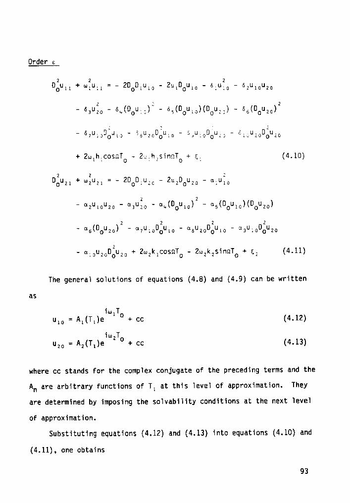
Order 2

2 2 * 3DOu1I.+ wlull =

_ZDODKULO

_ZHIDOUIÜ

_Ö1UlO - ÖZUIOUZO

' ösuäo

SBULOÜAULJU-

ÖLOUZODÄUZO

+ 2ulhlcosoTO — 2„;h,sinnTO + 5. (4.10)

2 2 _ 2Oouzl + wzuzl — - 2DODlu2G — 2u20Ou2Ü — alulo

2 2' GZULOUZO

‘°au2o

‘ °¤(DOU1o) ' “6(DOU1o)(DOU2o)

2 2 2 2“ ¤6(ÜOU20) “¤7Ul0DOul0 ' “6U2oDOUxo ' aauxoüouzo

(4.11)

The general solutions of equations (4.8) and (4.9) can be written

as

lw1TOulo = A1(T1)e + cc (4.12)

iw2TOuzo = A2(T1)e + cc (4.13)

where cc stands for the complex conjugate of the preceding terms and the

An are arbitrary functions of Tl at this level of approximation. They

are determined by imposing the solvability conditions at the next level

of approximation.

Substituting equations (4.12) and (4.13) into equations (4.10) and

(4.11), one obtains

93

2 2 , lw2TODouii + miuii (62 + 6Soiu2

2 — l(w —w )T Zlw T‘°

2 2lw2TOA2e + A6AiAi + A2A2A2

iolo+ ai(hi + ih2)e + cc + 51 (4.14)

2 2 lw2TÜOU2i + w2U2i = — 2lw2(A2 + u2A2)€

O- (ai

2 2 2 2iwiTo 2 2iw2TO- akwi — a2o2)Aie + A8A2e

- l(w2—wi)TO l(wi+w2)TO —+ A9AiA2e + A2oAiA2e + AiiAiAi

— inTO+ Ai2A2A2 + u2(ki+ ik2)e + cc + 52 (4.15)

where the prime indicates the derivative with respect to Ti and the

Ai are constants that depend on the values of the ai, 6i, and ai.

To proceed further, we need to specify the resonances being studied. In

this Chapter, we consider primary resonances of the second mode (i.e.,

Q = U2) in the presence of a two-to—one internal resonance (U2 = Zwi).

To describe quantitatively the nearness of these resonances, we

introduce the detuning parameters Si and S2 defined as

m2 = 2w2 + cgi, Q = w2 + 662 (4.16)

Using equations (4.16) to eliminate the terms that lead to secular terms

in equations (4.14) and (4.15) yields

94

, - allrl l 2„/al -1„l7¤2i(Al + plAl) + 4AlAlAze — E; fo gle dlo = 0 (4.17)

, 2 -1§l7l ißzrl2i(Az + pzAz) + 4AlA e (kl+ ikz)e

l~2'TT/{U2 *10.121-O

— ä; j gze dlo = 0 (4.18)“o

whereAl (4.19)

A=L(<1—1;-0.1.13) ·(420)2 4w2 1 7 1 '

It is convenient to express the An in equations (4.17) and (4.18)

in the form

1 i»lTl l ipzTlAl = ä (xl + iyl)e and Az = ä (xz + iyz)e (4.21)

whereV1 = (Vl + V2), V2 =

V2Substitutingequations (4.21) and (4.22) into equations (4.17) and

(4.18), separating real and imaginary parts, and replacing Tl with et,

we have

><; = nv. - ¤1><1+ ^1(v1><2 - wa) - gl (423)

yl = — vlxl - plyl + Al(xlxz + ylyz) - gz (4.24)

xz = vzyz - pzxz — 2Azxlyl + kz — gz (4.25)

2 2y; = - vzxz — uzyz + A2(xl — y,) — k, — 9. (4-26)

where

95

12H/wi

Q1= ZI E,iSln(wi+ cvl)t dt, (4.27a)0

127T/(.01

gz = ä; f ;icos(0; + 60i)t dt (4.27b)0

127T/M2

gz= ä; f ;,sin(0z+ 60z)t dt, (4.27c)' 0

12'TT/(J2

g„ = ä; f ;zcos(0z + 60z)t dt (4.27d)0

Starting from the averaged equations (4.23)-(4.26), we use the second-

order closure method to obtain some statistical measures of the coupled

motion.

4.3 Analysis i

we use the second—order closure method to determine the response

moments. To this end, we separate the xi and yi into the mean

components xio and yio and the random components xil and yil according

to

X1: X10 + X1.- v1= vi. + Y11 (4-28)

X2 : X20 + x21’ y2 = y2O + y21 (4°29)

Substituting equations (4.28) and (4.29) into equations (4.23)-(4.26)

and separating mean and fluctuating components, we find that the mean

motion is governed by

X10 = v1yl0 ‘ UIXIO + ^1(Y10X20 + <y11x21> ' x10y20 ' <X11y21>)(4.30)

96

V10 = ' v1X10 ' V1V10 + ^1(X1oX20 + <X11X21) + y10y20 + <V11V21))(4.31)

X20 = v2y20 ' V2X:a ' 2^:(X10V10 + <X11V11)) + X2 (4*32)

· 2 2 2 2y2O = ' V2X20 T UQVZQ + A2(X1O ’

V10 + (X11) ' <V11)) ' X1 (4'33)

Equations (4.30)—(4.33) show the presence of a feedback from the

fluctuations caused by the noise into the mean motion. This coupling

(terms in angle brackets) can be neglected if the random excitation is

small in comparison with the mean excitation as long as the parameters

considered are away from bifurcation values. we refer to this

assumption as the linearization method. To first order, the fluctuating

motion is given by

p = A p - g, (4.34)

where

' V1 ' ^1V20 V1 T AIXZO A1y10 ° ^1X10

' V1 + ^1X20 ' V1 + ^1y20 ^1X10 ^1y10A=

' 2^2V1o‘ 2^2X10 ' V2 V2

2Azx10 - 2Azy10 - vz - uz (4.35)

X11 gl= yll = 2 4 36p

Xog

(• )

21 gs.y21 gk

97

Ne note that A is a real nonsymmetric matrix.

The general solution of equations (4.34) can be obtained by modal

analysis. The eigenvalue and the adjoint eigenvalue problems of

equations (4.34) can be written as

TAp = Ap, A d = Ag (4.37)

The normalized modal matrices P and Q satisfy the conditions

QTP= I and QTAP = A (4.38)

where I is the identity matrix and A is a diagonal matrix whose elements

are the eigenvalues of the matrix A.

It is convenient to introduce a transformation that decouples

equations (4.34). To this end, we let

p = Pz (4.39)

Substituting equations (4.39) into equations (4.34), premultiplying by

QT, and using equations (4.38), we obtain

2m(t) = Amzm(t) + nm(t) for m = 1,2,3,4 (4.40)

where

4¤m(t) = - Z Q„m9„(t) (4-41)

n=l

and the Qmn are the elements of the modal matrix Q.

98

The statistics of the uncoupled coordinates zm are

<2m> = 0 (4.42)

(x t,+x t ) t t -(x 1 +) 1,)= 6 m "

2 f lf 26 m l"

“o o

for m,n = 1,2,3,4 (4.43)

where the angle brackets stand For the expectation.

As an example, we consider the case gl = 0 and 5, is a narrow-band

random excitation; that is,

5, = 2u,(F,cosnt - F,sinot) (4.44)

The modulations of F, and F, with time can be expressed as

6, + Q 66, = Q aw, , 6, + Q 66, = Q Bw, (4.45)

where 6 is the bandwidth of the random part of the excitation and w,

and w, are independent white noise. The autocorrelation Functions are

given by

< ) gsm < 46)R = R = S E 4•f1T) f2(T TT O

Substituting equations (4.41) into equations (4.43) and using equations

(4.46), we obtain the stationary mean—square values 0F the uncoupled

coordinates zm as

99

m nxm+xnfor

m, n = 1, 2, 3, and 4 (4.47)

Using equations (4.39) and (4.42), we obtain

5 5‘P1’ ‘

O-Fori, j = 1, 2, 3, 4 (4.48)

where the Pmn are the elements of the modal matrix P.

4.4 Results and Conclusions

Figure 4.1 shows the modal mean-square—response amplitudes as

functions of the mean-square excitations <F2>, where<F2>

= ¤S0. The

second mode is externally excited by a narrow-band random excitation

with a center frequency Q and a bandwidth 6. The case Q = dz is

considered. when<F2> < 0.167, the first mode is not excited and the

mean—square response of the second mode is proportional to the mean-

square excitation<F2>.

As<F2>

increases beyond 0.167, the mean-square

response of the first mode increases while <a;> remains 0.64 = constant

for all values of <F2>, indicating the existence of a saturation

phenomenon; that is, the directly excited mode is saturated and the

extra energy spills over into the indirectly excited mode. Increasing

the bandwidth of the narrow-band random excitation delays the start of

the nonlinear solution to<F2>

= 0.2, as shown in Figure 4.2. In Figure

4.3, we show the dependence of <ai> and <a;> on<F2>

for the case with a

100

multi—valued region. In addition to the saturation phenomenon, the

response curves display the jump phenomenon. In this case, two stable

solutions coexist when 0.284 s<F2>

s 0.385. In contrast to the linear

theory, the stationary response depends on the initial conditions when

more than one stable solution is possible. As <F2> increases from

zero, <a;> increases linearly with<F2>

while the first mode does not

respond as predicted by linear theory. when<F2>

= 0.385, <ai> jumps up

from zero to point B. As <F2 increases further, <ai> increases

nonlinearly with <F2> while <a;> remains 0.974=constant. As <F2>

decreases from point C, <ai> decreases along the curve CBA and <a;>

remains constant until point D. when <F2> decreases further, <ai> jumps

down to zero while <a;> jumps down to point E and decreases linearly

with <F2>.

Next, we study the effect of a low-intensity noise with a center

frquency 9 ¤ ul on the deterministic mean response. Representative

force—response curves are presented in Figure 4.4 when <F2> = 0. The

deterministic response exhibits the saturation phenomenon. For the case

<F2> representative force-response curves are presented in

Figure 4.5. when kl = 0, the first mode does not respond until kl

reaches the threshold value 0.008x10'3. As kl increases, the response

displays an energy exchange between the resonant modes. when kl 2

O.07x10'3, <a;> remains equal to 0.3 while <ai> increases with kl. This

indicates that the presence of the noise delays the start of the

saturation phenomenon from 0.05xl0_3 to 0.07x10'3. As a result,

increasing the bandwidth of the random excitation or adding a narrow-

101

band random excitation to a deterministic harmonic excitation delays the

onset of the saturation phenomenon. In other words, we are going toward

the white—noise extreme where the response does not display the

saturation phenomenon in the prsence of a two-to—one autoparametric

resonance (see Chapter 5). In Figure 4.6, we show frequency-response

curves when the second mode is excited by a deterministic harmonic and a

narrow-band random excitation. Nayfeh [162] indicated the possibility

of the nonexistence of stable periodic responses when -0.047 6 oi 6 -

0.0127 and<F2>

= 0, implying the existence of a Hopf bifurcation. In

the presence of the narrow-band noise, the second-order closure method

predicts a stable solution in this interval (i.e., all the eigenvalues

have negative real parts).I

In this Chapter, the second-order closure method is used to predict

the lower-order response moments of a two-degree-of—freedom system with

quadratic nonlinearities. According to the second-order closure method,

the response amplitudes xi and yi are separated into the mean components

xio and yio and the random components xil and yil. Next, the averaged

equations are separated into mean and fluctuating motions. This creates

a feedback from the fluctuations caused by the noise into the mean

flow. This coupling can be neglected if the random excitation is small

in comparison with the mean excitation (linearization method). However,

this coupling is necessary to give good approximations for the mean-

square responses at the boundary between stable and unstable periodic

motions.

102

CHAPTER 5

CUMULANT-NEGLECT CLOSURE FOR SYSTEMS HITH MODAL INTERACTIONS

Statistical response moments of two—degree—of-freedom systems with

quadratic and cubic nonlinearities to zero-mean Gaussian white noise are

determined. The cases of two—to-one, one—to—one, and three—to-one

internal resonances are investigated. Ito stochastic calculus is used

to derive general first—order ordinary—differential equations describing

the evolution of the response moments. The response-moment equations

are an infinite hierarchy set due to the nonlinearities. Gaussian and

non—Gaussian closure schemes are used to close this set, leading,

respectively, to 14 and 69 equations for the lower—order response

moments. Guided by the results of the method of multiple scales for the

deterministic case of internally resonant oscillators, we reduce the

number of response-moment equations for the case of non—Gaussian closure

by approximately a factor of two. The results obtained by the reduced

scheme are in excellent agreement with those obtained by the full 69

equations. The results reveal major discrepancies between the Gaussian

and non—Gaussian closure schemes. Close to internal resonance,

stationary bi—modal solutions exist and energy shifts between the two

modes. However, the response does not display the saturation phenomenon

for the case of a two—to-one internal resonance, The results are

applied to a shallow arch, a string, and a hinged-clamped beam.

103

5.1 Introduction

In this Chapter we consider two-degree—of-freedom systems governed

by equations of motion having the form

ui + wiui + 2plui+ 3iiui+ ßziuiuz + giiului + guiui

+ 6iUi + szuiul + aiui + 6Luä + Bsuiuz (5.1)

dz

asuiuz + asüä = g2(t) (5.2)

where the ui, ui, Bil, Biz, 6i, and ai are constants, the overdots

denote derivatives with respect to time, and the gi are zero-mean

Gaussian white noise whose auto-correlation functions are given by

RE (1) Rg (1) = 21S,6(1), and Rg g (1) = 21Si26(1) (5.3)1 2 1 2

The following discussion provides a brief background of the present

Chapter. For a comprehensive review, the reader is referred to the

textbooks by Nayfeh and Mook [163] and Ibrahim [178].

Ariaratnam [179] used the Markov procedure to determine the random

response of two-degree—0f-freedom vibrating isolating suspensions with

cubic displacement-dependent nonlinearities. For some special

conditions, he obtained exact steady-state solutions of the Fokker-

Planck-Kolmogorov equation. Bhandari and Sherrer [180] investigated the

probabilistic behavior of systems with both displacement- and velocity-

dependent nonlinearities. They represented the steady—state

104

probability-density function in terms of multiple series of Hermite

polynomials. They used Galerkin‘s method to determine the coefficients

of the series. They considered 81 terms in the series expansion to

achieve a reasonable agreement with the results obtained by the exact

solution of the FPK eguation.

Ibrahim and Roberts [181l used the Gaussian closure scheme for

investigating the response moments of a two-degree-of—freedom system

with quadratic nonlinearities. In the neighborhood of a two—to—one

internal resonance, the Gaussian closure scheme did not yield fixed-

point response moments. Their results show a suppression effect on the

higher mode and large random motions of the coupled system. Ibrahim and

Roberts [182l analyzed the effect of the system parameters on the

stability of the stationary uni-modal response of the higher mode. The

experimental results of Roberts [183] indicate wider instability regions

than those predicted by analytical methods. Ibrahim and Heo [184]

compared the results obtained by the Gaussian-closure scheme with those

obtained by the non-Gaussian closure scheme. Contrary to the Gaussian

closure results, the non-Gaussian closure analysis yields complete

fixed-point response moments. Ibrahim and Sullivan [185] conducted an

experimental investigation of the response of a two-degree-of—freedom

structural model possessing a two-to-one internal resonance to band-

limited random excitations. Their results did not indicate the

existence of saturation.

In this Chapter, three closure schemes are used to determine the

response moments of two-degree-of—freedom systems possessing internal

105

resonances to zero—mean Gaussian white noise. They are the Gaussian,

non—Gaussian, and reduced non-Gaussian closure schemes. The cases of

two—to-one, three—to—one, and one-to-one internal resonances are

treated. The method of multiple scales is used to establish the

response characteristics and its narrow-band nature. This information

is utilized to reduce the response-moment equations of the non—Gaussian

closure scheme by about a factor of two. The results obtained by the

Gaussian closure scheme do not agree with those obtained by the non-

Gaussian closure scheme. Close to resonance, the results show energy

exchanges between the two modes. As applications of the present

results, we investigate the responses of a shallow arch, a string, and a

hinged—clamped beam to broad-band random excitations.

5.2 Closure Schemes via the Markov Procedure

Equations (5.1) and (5.2) can be written as

dx, = x,dt, dx, = x„dt, (5.4)

dx.dN, (5.5)

dx.dN, (5.6)

where

x, = u,, x, = u,, x, = u, and xk = ü, (5.7)

106

gi = dNi/dt (5·8)

Here, the Ni(t) are Brownian processes. Equations (5.4)-(5.6) are of

Ito type and {xl, xl, xz,x_‘

constitutes a four—dimensional Markov

vector. Using Ito stochastic calculus [186], we use equations (5.4)-

(5.6) to derive the response moments. To this end, we let

_ < 1 1 k 1) _f“ f“ f“ f“

1 3 k 1 _tmi j k’2 - - p(x1,x2,x3,x„, )

dxldxzdxgdxä (5.9)

The Fokker-Planck—Kolmogorov equation associated with equations (5.4)-

(5.6) can be written as

6 6 6 6 2 3 35% = — X. 5% - X.5%2

3 2 2 2+ B31X1X2 + BQIXZ + 61xx + 62XlX2 + öaxz + öuxa + ösxsxu

2 2 3 2 2

812Xl+ ß22X1X2 + Bazxxxz

3 2 2 2 2+ ßwzxz + alxl + ¤2X1X2 + aaxz + auxa + asxsxn + °6X¤)p]

2 2 2

«S2 2-% (5.10)

The response-moment equations of any order n (n = i + j + k + 1) can be

obtained by multiplying equation (5.10) by xixgxäxä and integrating by

parts over the whole state space. Hence, the response moments of any

order are governed by

107

dm. .1,},k,z = . . 2at ‘m1-1,3,k+1,1 * Jm1,j-1,k,1+1 ‘ k[“im1+1,5,k-1,1

* B3lmi+1,j+2,k—1,1 * ß~¤m6,5+2,k-1,1 * 61mi+2,j,k—1,z * 62mi+1,j+1,k—1,2

+ ö6mi,j,k-1,1+2]” Q [“£mi,j+1,k,m-1 + 2“2mi,j,k,2

* B12mi+3,j,k,2—1 + “22m1+2,5+1,k,1-1 * B32mi+1,j+2,k,1-1 * “~2m1,5+2,k,1-1

* °1m1+2,5,k,1-1 * “2m1+1,g+1,k,1-1 * °2m1,5+2,k,1-1

j j(5.11)

Equation (5.11) shows that a statisticai moment equation of order n

contains moments of order 2 n+2. Hence, the statisticai response

moments are governed by an infinite hierarchy set. C1osure schemes are

usua11y employed to truncate this set and approximate the important

1ower—order moments.

108

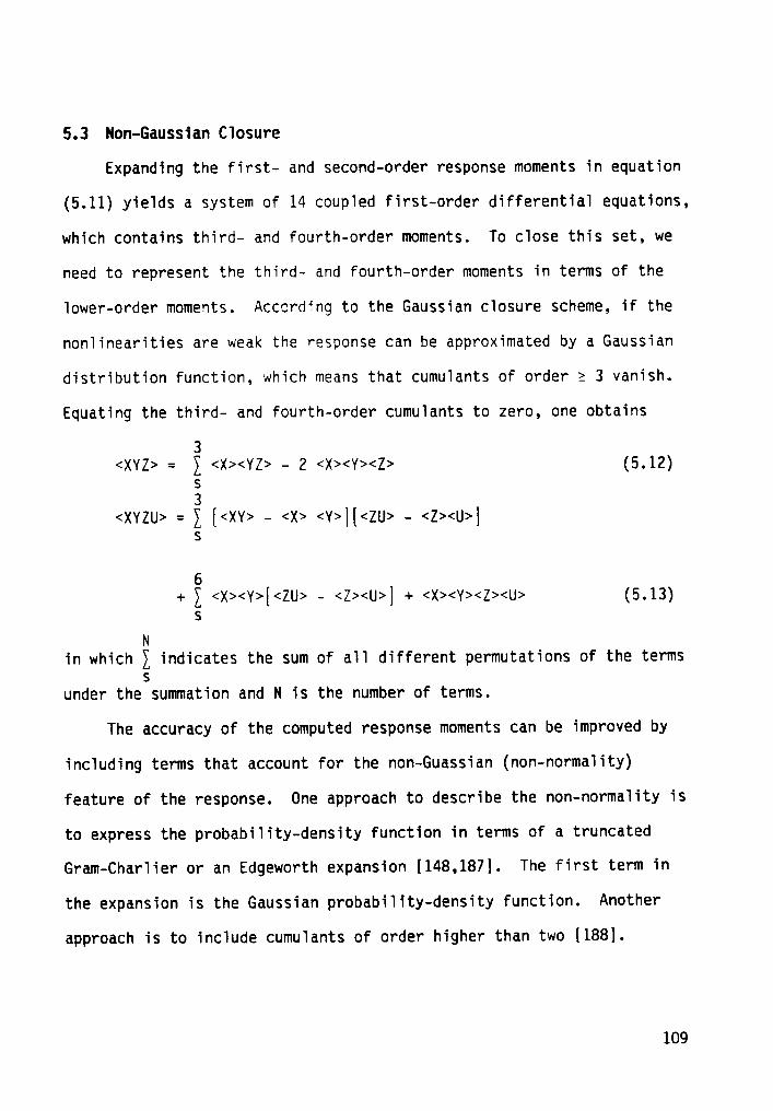
5.3 Non—Gaussian Ciosure

Expanding the first- and second—order response moments in equation

(5.11) yieids a system of 14 coupied first-order differentiai equations,

which contains third- and fourth-order moments. To close this set, we

need to represent the third- and fourth-order moments in terms of the

Tower-order moments. According to the Gaussian ciosure scheme, if the

noniinearities are weak the response can be approximated by a Gaussian

distribution function, which means that cumuiants of order 2 3 vanish.

Equating the third- and fourth-order cumuiants to zero, one obtains

3<XYZ> = 2 <X><YZ> - 2 <X><Y><Z> (5.12)

s

<xYZU> <x> <v>][<Zu> - <Z><U>]s

6+ E <x><Y>[<ZU> - <Z><U>] + <x><Y><Z><U> (5_13)

s

Nin which Z indicates the sum of ali different permutations of the terms

under thessummation and N is the number of terms.

The accuracy of the computed response moments can be improved by

inciuding terms that account for the non-Guassian (non—norma1ity)

feature of the response. One approach to describe the non—norma1ity is

to express the probabi1ity—density function in terms of a truncated

Gram-Chariier or an Edgeworth expansion [148,187]. The first term in

the expansion is the Gaussian probabiiity-density function. Another

approach is to inciude cumuiants of order higher than two [188].

109

Expanding the response moments of order s 4 in equation (5.11)

yields a system of 69 coupled first—order differential equations, which

contains fifth— and sixth-order moments. To close this set, we express

the fifth- and sixth-order moments in terms of the lower—order

moments. To this end, we equate fifth- and sixth-order cumulants to

zero; that is,

5 10 10<XYZUV> = E <X><YZUV> — 2 1 <X><Y><ZUV> + 6 Z <X><Y><Z><UV>

s s s15 10

- 2 E <XY><ZU><V> + E <XY><ZUV> - 24 <X><Y><Z><U><V>

S S (5.14)

6 15<XYZUVW> = Z <X> <YZUVw> — 2 1 <X><Y><ZUVw>

s s20 15

+ 6 E <X><Y><Z><UVw> - 24 E <X><Y><Z><U><Vw>

s s15 10 45

+ Z <XY><ZUVw> + E <XYZ><UVw> + 6 E <X><Y><ZU><Vw>s s s

15 60- 2 E <XY><ZU><Vw> - 2 E <X><YZ><VUw> + 129 <X><Y><Z><V><U><w>

s s

(5.15)

Next, we use the method of multiple scales to describe the nature

of the response and its characteristics. Ne utilize this information to

reduce the 69 response—moment equations derived via the non-Gaussian

closure scheme. The cases of two-to—one, one-to-one, and three-to—one

internal resonances are investigated.

110

5.4 Two-To—0ne Internal Resonance

Ne describe the nearness of the two-to-one internal resonance by

introducing the detuning parameter o defined according to

mz = Zm1 + v (5.16)

To the first approximation, the general solution of equations (5.1) and

(5.2) can be expressed in terms of two narrow—band random processes with

the center frequencies mg and ä mz; that is,

1 . 1u1 z x1cos (5.17)

u2 = X2C0Sm2t — y2sinm2t (5.18)

· 1 . 1 1 5 19U102

= — m2(x2sinm2t + yzcosmzt) (5.20)

where the x1 and yi are slowly varying random functions governed by

x = - u x + L vy + A (y x - x y ) - l- 5 sin(l m +·l o)t (5.21)1 1 1 2 1 1 1 2 1 2 M1 1 2 2 2

y = - p y - L vX + A (x x + y y ) — l- 5 cos(l m + L v)t (5.22)1 1 1 2 1 1 1 2 1 2 wl 1 2 2 2

x2 = - pzxz - 2A2x1y1 - é- gzsinmzt (5.23)2

. 2 2 1yz = - uzyz + A2(x1 - y1) 52cosm2t (5.24)

the underbars denote short-time averaging over the period 21/mz, and

1 l 2A1 (62 + m1m2•S5) , A2 (o11 (5.25)

111

The response-moment equations (5.11) involve short- and long-time

averaging. The former kills fastly varying quantities. Substituting

equations (5.17)-(5.20) into equations (5.9) and performing short-time

averaging, we find that 38 out of the 69 moments are zero. As an

example, we consider

ui = (xzcosblt + y3sind3t)E

m2 3 3 2 Z= ä; [x, fo cos dzt dt + 3x2y2fO cos wzt sinuzt dt

3 Zn/m2 3 3 Zw/bz 3+ 3x2y2 f cosuzt sin dlt dt + yz f sin wat dt] = 0 (5.26)

o o

For the case oz = 2w,, the zero-response moments are given in Appendix

III.

Transition and steady-state solutions of the response—moment

equations are obtained by numerically integrating the coupled response-

moment equations by a fifth—order Runge—Kutta-Verner technique. Results

are presented showing the variation of the mean-square responses with

internal detuning, excitation spectral amplitude, and time.

Numerical integration of coupled differential equations or solving

systems of simultaneous algebraic equations is time consuming and

deperds significantly on the number of these equations. Guided by the

narrow-band nature of the response of lightly damped systems, we reduce

the number of the coupled response—moment equations generated by the

112

non-Gaussian closure scheme. Consequently, computer time is drastically

reduced.

The variation of the mean—square responses with the detuning

parameter v is shown in Figure 5.1 when gl = O. The results of the

non—Gaussian closure scheme are in good agreement with those obtained by

using the reduced non—Gaussian closure scheme. In the neighborhood of a

perfectly—tuned autoparametric resonance, the response exhibits an

energy exchange between the two modes. Away from the autoparametric

resonance, the effect of the coupling dies out and a uni-modal response

is displayed. when v = O, Figure 5.2 shows the effect of the spectral

amplitude S2 of the excitation on the mean—square responses. These

results do not indicate the existence of saturation.

For the case of a perfectly tuned system (i.e., oz = 2ul and v =

O), Figure 5.3 shows that the Gaussian closure technique predicts a uni-

modal response consisting of the directly excited second mode and that

the unexcited first mode does not respond. Adding the third- and

fourth-order cumulants and equating the higher-order cumulants to zero

can help describe part of the non—Gaussian feature of the response due

to the nonlinearities. Figure 5.4 shows the modulation of the mean-

square response with time for the case oz = 2ul. It shows that the

non—Gaussian closure scheme predicts a bi-modal response, in contrast

with the Gaussian closure scheme, which predicts a uni-modal response.

113

The directly excited second mode passes part of the energy it receives

to the indirectly excited first mode due to the autoparametric

resonance. _

Beyond a transition period, Figure 5.5 shows that the Gaussian

closure scheme does not yield long-time fixed—point response moments as

reported by Ibrahim and Roberts [181].

As an application, we consider the nonlinear response of an arch to

a random excitation. The equation of motion of a hinged—hinged arch

with a rise wO(x) is given by [189 ]

M 2 2gzw

EI 2-% + oA 2-% + c %% - N (2-% + ——%2) = Q(x,t) (5.27)ax 7at ax ax

w = 0 and 2;% = 0 at x = 0,L (5.28)ax

where

(nä T; (5.29)

Here, w(x,t) is the transverse displacement, E is Young's modulus, A and

I are the area and moment of inertia of the cross section, p is the

density, L is the projected length, c is the damping coefficient, and Q

is the transverse load.

we consider the case of a sinusoidal rise and expand w in terms of

the undamped free linear vibration modes; that is,

w(x,t) = 2r ä un(t) sin B22 (5.30)n=1

wO(x) = 2ri

xnsin 2%% (5.31)n-1

114

where r is the radius of gyration of the cross section. Using

Galerkin's method, assuming modal damping, and truncating the result for

two modes, we obtain equations (5.1) and (5.2) where

62 = 261 + 6 (5.32)

and the system parameters are given by Nayfeh [189].

As an example, we let x1 = 5.35 and x2 = 0.26 so that 61 = 1.0, 62

= 2.0, 611 = 0.092, 621 = — 0.172, 621 = 0.368, 6,1 = — 0.184, 612 = -

0.057, 622 = 0.368, 622 = — 0.552, Bkz = 0.953, 61 = 1.275, 62 = —

0.986, 62 = 1.328, 61 = - 0.493, 62 = 2.656, and 62 = 0.250. we are

primarily concerned with low—amplitude motions. Consequently we let

un = Eu; (5.33)

where 6 is a measure of the motion amplitude.

Figure 5.6 shows the variation of the mean-square responses with

the internal detuning parameter 6. The first and second modes are

externally excited by two uncorrelated zero—mean white noise. Their

spectral amplitude excitations are related by the following equation:

gi — Ei = 0 (5.34)U) U2

The results of the non-Gaussian closure scheme are in good agreement

with those obtained by using the exact stationary solution of the FPK

equation. For the case 62 = 261, Figure 5.7 shows the modulation of the

mean—square responses with time when the first mode is excited by a

· 115

zero-mean Gaussian white noise. The non-Gaussian closure scheme

predicts a bi-modal response. Variations of the mean—square responses

with the internal detuning parameter o are presented in Figure 5.8. In

the neighborhood of o = 0, the response exhibits an energy exchange

between the two modes. The minimum mean—square response of the directly

excited mode and the peak mean-square response of the indirectly excited

mode occur when o < O. This indicates a softening nonlinearity. As

|o| increases, the effect of the autoparametric resonance decreases and

finally a uni-modal response is displayed.

5.5 One-To-One Internal Resonance

Using the method of multiple scales, one finds that, to the first

approximation, the general solution of equations (5.1) and (5.2) can be

expressed in terms of two narrow-band processes with the center

frequency mz; that is,

ui = xicosuzt — yisinwzt for i = 1, 2 (5.35)

In this case, we find that 24 out of the 69 moments are zero. The zero-

response moments are given in Appendix IV.

Figure 5.9 shows the dependence of the mean—square responses on the

internal detuning parameter o. Both modes are externally excited by

zero-mean Gaussian white noise. The response curves are single-valued

functions for all values of o. The results of the non-Gaussian scheme,

the reduced scheme, and those obtained by using the exact stationary

solution of the FPK equation are in good agreement. when o = U2 - ol =

116

0, Figure 5.10 shows the time history of the mean-square responses. The

response—moment equations asymptote constant values (fixed-point

solution) (i.e., gTiä%¢6L£ = 0). For some parameters, a false fixed-

point solution might be reached. In this case, the time history

displays a fixed-point solution for some time and then shows a jump to

another solution. Hence, caution must be exercised to establish a true

fixed-point solution by integrating for sufficiently long times.

Variations of the mean—square responses with the detuning

parameter o are presented in Figure 5.11. Comparisons of the results of

the non—Gaussian-closure and those obtained by using the reduced non-

Gaussian closure scheme are in excellent agreement. The response curves

are single-valued functions for all values of o. when o = 0, the

response displays an energy exchange between the two resonant modes.

As lol increases, the effect of the internal coupling vanishes and the

system displays a uni—modal response.

As an application, we consider the nonlinear response of a string

to a random excitation. The equations of motion of a string with an

initial tension No are given by [163]

azu 2 azu 2 2 2 1 au av 2 aw 2ggg — C2 ggg = (Cl · C2) gg [[5 · gg ll(gg) + (gg) ll (6-36)

azv 2 azv 2 2 6 av au au 2 1 av 2 1 aw 2ggg * C2 ggg = (C] * C2) gg [gg [gg · (gg) + 5 (gg) + 5 (gg) ll

(5.37)

azw 2 azw 2 2 a aw au au 2 1 av 2 1 aw 2**g — C2 **g = (C] - C2) gg [gg [gg — (gg) + 5 (gg) + 5 (gg) ll8* 2 8* (5.38)

u = v = w = O at x = 0, L (5.39)

117

where u is the longitudinal displacement and v and w are the transverse

displacements. Here, cl and c, are the longitudinal and transverse

speeds of sound given by

Cl = ./Üb- and C‘ = (5.40)

Neglecting the longitudinal inertia 2~%, considering the first mode- at

in each of the transverse motions, adding modal damping forces and

external broad—band random excitations, expanding v and w in terms of

the linear free undamped modes, and using Galerkin's method, we obtain

~ 2 . 2 2ul + alu, + 2ulU1 + rul + ruluz = ;1(t) (5.41)

~ 2 . 2 2u2 + wzuz + Zuzuz + ru, + ruluz = ;,(t) (5.42)

where

012 = ml + v (5.43)Q 2

nC2 w Clw1= dhd I' = jj (5.44)

4L

Figure 5.12 shows that the results of the non-Gaussian closure

scheme are in excellent agreement with those obtained by using the exact

stationary solution of the FPK equation. For the case of a perfectly

tuned system (i.e., oz = ul), Figure 5.13 shows that the non—Gaussian

closure predicts a uni-modal response. As the linear damping parameters

decrease, Figure 5.14 shows that the response exhibits an energy

exchange between the two modes. Similarly, increasing the spectral

118

amplitude of the excitation results in a bi—modal response, as shown in

Figure 5.15. Variations of the mean—square responses with the

excitation spectral amplitude S1 are presented in Figure 5.16.

For Sl < 0.035, the response displays a uni—modal response.

For Sl 2 0.035, the response starts to display an energy exchange

between the two internally-resonant modes. The response of the

unexcited second mode builds up due to the presence of the nonlinear

coupling. Figure 5.17 shows the dependence of the mean—square responses

on the internal detuning parameter u when the first mode is externally

excited by a zero-mean Gaussian white noise. The results of the non-

Gaussian closure scheme are in excellent agreement with those obtained

by using the reduced scheme. The energy—exchange peak between the two

resonant modes occurs when u > 0. This indicates a hardening

nonlinearity. Away from the autoparametric resonance, the effect of the

nonlinear coupling decays and the response displays a uni—modal

response.

5.6. Three-To—0ne Internal Resonance

Using the method of multiple scales, one can show that, to the

first approximation, the response is given by narrow—band processes with

the center frequencies ä oz and oz; that is,

ul = xlcos ylsin u, = xzcoswzt - yzsinwzt (5.45)

In this case, we find that 36 out of 69 moments are zero. The zero-

response moments are given in Appendix V.

119

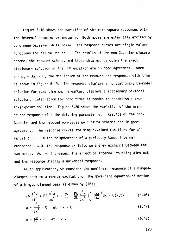
Figure 5.18 shows the variation of the mean-square responses with

the internal detuning parameter v. Both modes are externally excited by

zero-mean Gaussian white noise. The response curves are single-valued

functions for all values of o. The results of the non-Gaussian closure

scheme, the reduced scheme, and those obtained by using the exact

stationary solution of the FPK equation are in good agreement. when

v = mz - 3ul = 0, the modulation of the mean-square responses with time

is shown in Figure 5.19. The response displays a nonstationary bi-modal

solution for some time and hereafter, displays a stationary bi-modal

solution. Integration for long times is needed to establish a true

fixed-point solution. Figure 5.20 shows the variation of the mean-

square response with the detuning parameter o. Results of the non-

Gaussian and the reduced non-Gaussian closure schemes are in good

agreement. The response curves are single-valued functions for all

values of v. In the neighborhood of a perfectly-tuned internal

resonance v e 0, the response exhibits an energy exchange between the

two modes. As lvl increases, the effect of internal coupling dies out

and the response display a uni-modal response.

As an application, we consider the nonlinear response of a hinged-

clamped beam to a random excitation. The governing equation of motion

of a hinged-clamped beam is given by [163]

pA AAA + EI AAA + c AA - E5 AAAfL

(AA)2dx = Q(x t) (5.46)atz

axkat 2L axz

o ax’

w = AA; = 0 at x = 0 (5.47)ax

w = gg = 0 at x = L (5.48)

120

Ne expand w(x,t) in terms of the undamped free 1inear modes; that is,

2 YZ)

w(x,t) ={- Z ·¤n(:<)un(t) (5.49)n=l

where

_ 2 . .¢n(x) - ———-1;-——————;—-——— [sin(xnx)s1nh(1nL)

sinh (xnL)-sin (xnL)

- sin(xnL)sinh(xnx)] (5.50)

tan(xnL) - tanh(xnL) = 0 (5.51)

and the eigenvaiues of the first and second mode are

AIL = 3.9266, 12L = 7.0686 (5.52)

Considering the first and second mode, assuming moda1 damping, and using

Ga1erkin's method, we obtain

·· 2 . 3U1+ w1U1+ 2U1Ul+ Erllllul + E(F1112 + I:1121

2 2

+ erlzzzuä = ;1(t) (5.53)

·· 2 . 3U2 + ")2U2 + zuzuz + €r211lu1 + E(r2112 + I‘212l

2 2+ F221l)u1u2 + €(r2122 + {.2212 + r2221)u1U2

+ erzzzzui = ;2(t) (5.54)

121

where

oz = 3ul + v (5.55)

rmnkl = L2]f; ¢m ä;%Ü dx fg ääi ;;& dx] (5.56)

Figure 5.21 shows the variation of the mean—square responses with

the excitation spectral amplitude S1 when both modes are externally

excited by two uncorrelated zero-mean Gaussian white noise. The results

of the non-Gaussian closure scheme are in good agreement with thoseV

obtained by using the exact stationary solution of the FPK equation.

Figure 5.22 shows the dependence of the mean—square responses on the

excitation spectral amplitude Sl when the first mode is externally

excited by a zero-mean Gaussian white noise. The results obtained by

using the reduced non-Gaussian scheme are in good agreement with those

obtained in the non-Gaussian scheme. As S1 increases, the response

displays an energy exchange between the two resonant modes. The

directly excited first mode passes part of the energy it receives to the

indirectly excited second mode due to the autoparametric resonance.

5.6 Conclusions

Three cumulant-neglect closure techniques are used to determine the

important lower-order response moments of two—degree—of-freedom systems

with quadratic and cubic nonlinearities to external zero-mean Gaussian

broad-band excitations. They are the Gaussian, non—Gaussian, and

reduced non—Gaussian closure schemes. The cases of two—to-one, one—to—

122

one, and three-to-one internal resonances are investigated. The Markov

vector procedure is used to obtain general first-order ordinary-

differential equations governing the evolution of the response

moments. The nonlinearities result in an infinite heirarchy set for the

response-moment equations. Gaussian and non-Gaussin closure schemes

yield, respectively, 14 and 69 equations for the lower-order response

moments. Numerical integration of these coupled differential equations

or solving the corresponding system of simultaneous algebraic equations

(i.e., ETiä%lE¢& = 0 ) is time consuming and depends significantly on

the number of these equations. The method of multiple scales is used to

describe the nature of the response and its characteristics. This

information is utilized to reduce the number of the coupled response-

moment equations generated via the non-Gaussian closure scheme.

Consequently, computer time is drastically reduced. The results

obtained by using the reduced scheme are in good agreement with those

obtained by using the full 69 equations. The results are applied to

determine the nonlinear responses of a shallow arch, a string, and a

hinged-clamped beam to broad-band random excitations. Close to

autoparametric resonance, the responses display an energy exchange

between the interacting two modes. However, the response does not

display the saturation phenomenon predicted for deterministic harmonic

excitations in the case of two-to-one internal resonances. The results

reveal major discrepancies between the Gaussian and non-Gaussian closure

schemes. The Gaussian closure scheme does not yield stationary

response moments.

123

CHAPTER 6

CONCLUSIONS AND RECONMENDATIONS FOR FUTURE WORK

In this dissertation we develop three methods to study the response

of nonlinear systems to combined deterministic and stochastic

excitations. They are a second—order closure method, a generalized

method of equivalent linearization, and a reduced non—Gaussian closure

scheme.

An effective method for determining the response of nonlinear

systems to random excitations is to consider a set of equations for the

moments of the response. This yields important response statistics,

such as means and variances. The response—moment equations are an

infinite heirarchy set due to the nonlinearities. Moment closure

schemes are used to close this set. After a transformation from the

fastly varying state vector {u, u}T to the slowly varying

vector {A,6}T, we propose a second—order closure method to determine the

first- and second-order response moments in Chapter 1. In this method,

we take the following steps. First, we use the method of multiple

scales to determine the equations describing the modulation of the

amplitude and phase with the nonlinearity and excitation. Second, we

separate the averaged equations into mean and fluctuating components.

Third, we use these equations to obtain closed-form expressions for the

stationary mean and mean-square response. It is found that the presence

of the nonlinearities causes multi—valued regions where more than one

mean-square value of the response is possible. The multi-valuedness is

responsible for a jump phenomenon. The local stability of the

124

stationary mean and mean-square response is analyzed. For some range of

parameters, the presence of noise can expand the stability region of the

deterministic mean motion. The second—order closure method attacks the

problem in a way that the statistics of the response can be obtained for

general types of excitation and nonlinearity.

The method of equivalent linearization is based on replacing the

nonlinear governing equations of motion by equivalent linear equations

whose solution furnishes an approximate solution to the nonlinear

response. The equivalent linear parameters are determined by minimizing

the mean-square value of the difference between the two sets of

equations. In achieving this goal, the method of equivalent

linearization creates many limitations and overlooks many interesting

phenomena introduced by the presence of the nonlinearities. A

generalization of the method of equivalent linearization is presented in

Chapter 3. The original nonlinear governing equation is replaced by two

equivalent linear equations. This method provides some means to

describe the non—Gaussian feature of the nonlinear response and

preserves its wide-band character. The interaction and feedback between

the nonlinearity and excitation create nonlinear resonances. These lead

to linear shifts in the frequency and damping and an adjustment of the

strength of the primary excitation. The former is responsible for the

increase in the modal frequency and the latter contributes to the

experimentally observed broadening of the response curves. To test the

soundness of the proposed method, it is used to determine the mean-

square response of the Duffing and Van der Pol—Rayleigh oscillators to a

125

Gaussian white noise and a superharmonic narrow-band random excitation

of order three. For the former, it is shown that the proposed method

yields a better approximation to the mean-square response than the

method of equivalent linearization. For the latter, the method of

equivalent linearization predicts a single-valued function for the mean-

square response. However, the proposed method predicts multi-valued

regions where more than one mean-square value of the response is

possible.

In Chapter 4 the second—order closure method is used to analyze the

response of two-degree-of—freedom systems with quadratic nonlinearities

to narrow-band random excitations. The case of primary resonance of the

second mode in the presence of a two—to—one internal (autoparametric)

resonance is investigated. Contrary to the results of the linear

analysis, the nonlinear analysis reveals that the directly excited

second mode takes a small amount of the input energy (saturates) and

spills over the rest of the input energy into the first mode, which is

indirectly excited through the modal coupling.

Three closure schemes via the Markov vector procedure are used to

determine the lower—order statistical response moments of two-degree-of-

freedom systems with quadratic and cubic nonlinearities in Chapter 5.

They are the Gaussian, non-Gaussian, and reduced non—Gaussian closure

schemes. The system is externally excited by zero-mean Gaussian white

noise. The case of two-to-one, one-to-one, and three-to-one

autoparametric resonances are investigated. Ito stochastic calculus is

used to derive a hierarchy set of first-order differential equations

126

governing the modulation of the response moments with time. Gaussian

and non-Gaussian closure schemes are used to close this set, leading,

respectively, to 14 and 69 equations for the lower-order response

moments. The method of multiple scales is used to describe the nature

of the response and its characteristics. This information is utilized

to drastically reduce the number of the response-moment equations

generated by using the non-Gaussian closure scheme. The results

obtained by using the reduced scheme are in excellent agreement with

those obtained by using the full 69 equations. Close to autoparametric

resonance, the response displays an energy exchange between the two

modes. The response, however, does not display the saturation

phenomenon predicted for the case of two-to-one internal resonances.

The results reveal major discrepancies between the Gaussian and non-

Gaussian closure schemes. The results are applied to a shallow arch, a

string, and a hinged—clamped beam.

In any extension of the work presented in this thesis, the

following points are noteworthly:

1. The second-order closure method can be used to determine the

response of two-degree—of-freedom systems with cubic nonlinearities

to non-zero mean random excitations in the presence of one—to-one

and three—to-one autoparametric resonances.

127

2. An attempt to introduce some correlation between fl and fz in the

generalized method of equivalent linearization is expected to yield

a better solution.

3. Extenson and application of the methods indicated in this thesis to

stationary non—Gaussian, nonstationary Gaussian, and nonstationary

non—Gaussian random excitations are still needed.

4. Future studies need to be directed at investigating the stability

of the response of dynamical systems to non-zero mean random

excitations by examining the perturbed state equations.

5. The three methods developed in this study can be applied to

determine the response of many elastic and dynamical structures,

such as plates, shells, ships, and foundations. Extensions to

composite structures are also recommended.

6. The fact that our theoretical results are based upon approximate

methods points out the need for supporting experimental

investigations.

128

REFERENCES

1. R. H. LYON 1963 J. Acoust. Soc. Amer. 35, 1712-1721. Empirical

evidence for nonlinearity and directions for future work.

2. S. H. CRANDALL 1974 Shock Vib. Dig. 6, 2-14. Nonlinearities in

structural dynamics.

3. J. B. ROBERTS 1976 ASCE J. Engrg. Mech. Div. 102, 851-866. First

passage probability for nonlinear oscillators.

4. J. 8. ROBERTS 1978 J. Appl. Mech. Trans. ASME 45, 175-180. First

passage time for oscillators with nonlinear damping.

5. J. B. ROBERTS 1978 J. Sound Vib. 56, 71-86. First passage time for

oscillators with nonlinear restoring forces.

6. M. C. NANG and G. E. UHLENBECK 1945 Rev. Mod. Phys. 17, 323-342. On

the theory of Brownian motion II.

7. A. T. BHARUCHA-REID 1960 Elements of the Theory of Markov Processes

and Their Applications. New York: McGraw Hill.

8. R. D. CLOUGH and J. PENZIEN 1975 Dynamics of Structures. New York:

McGraw Hill.

129

9. S. H. CRANDALL and W. D. MARK 1963 Random Vibration in Mechanicai

Systems. Academic Press.

10. Y. K. LIN 1973 Probabiiistic Theory of Structurai Dynamics. New

York: McGraw-Hill.

11. A. EINSTEIN 1905 Ann. Phys. (Leipzig} 17, 549-560. Uber dievan der

moiekuiar-kineteschen theorii der warme gefordert bewegung von in

ruhenden fiussigkeiten.

12. A. P. FOKKER 1914 Annais. Phys. 43, 810-815. Die mittiere energie

rotierender eTectricher dipoie im stahTungsfe1d.

13. M. PLANCK 1917 Stizungsber. Preuss. Akadamie weiss, 324-341. Uber

einen Satz der Statischen Dynamik und Seine Erweiterung in der

Quanten-Theorie.

14. N. FELLER 1936 Math. Ann. 113, 133-160. Zur theorie der

stochastischen prozesse (existenz und eindeutigkeitssatze).

15. K. IT0 1946 Proc. Jap. Acad. 22, 32-35. 0n a stochastic integrai

equation.

130

16. K. IT0 1951 Mem. Amer. Math. Soc. 4, 51-59. On stochastic

differentiai equations.

17. J. L. DOOB 1953 Stochastic Processes. New York: Wiiey.

18. A. KOLMOGOROV 1931 Mathematische Annaien 104, 415-458. Uber die

anaiytischen methoden in wahrsheiniichkeitsrechnung.

19. PONTRIGIN, ANDRANOV, WITT 1933 Zh. eksg. teor. Fix. 3. A

statisticai review of dynamic systems.

20. K. CHUANG and L. F. KAZADA 1959 Trans. AIEE 78, 100-105. A study of

noniinear systems with random inputs.

21. S. T. ARIARATNAM 1960 J. Mech. Engrg. Sci. 2, 195-201. Random

vibrations of noniinear suspensions.

22. R. H. LYON 1960 J. Acoust. Soc. Amer. 32, 716-719. On the vibration

statistics of a randomiy excited hard-spring osciiiator.

23. T. K. CAUGHEY 1971 Adv. Aggi. Mech. 11, 209-253. Noniinear theory

of random vibrations.

131

24. W. D. IWAN 1974 Appi. Mech. Earthquake Engrg., Proc. Winter Mtg.

ASME, ASME/AMD 8, edited by W. D. Iwan, 135-161. Appiication of

noniinear anaiysis techniques.

25. D. LUDWIG 1975 SIAM Rev. 17, 605-640. Persistence of dynamicai

systems under random perturbations.

26. M. F. DIMENTBERG 1982 Int. J. Noniin. Mech 17, 231-236. An exact

soiution to a certain noniinear random vibration probiem.

27. T. K. CAUGHEY and F. MA 1982 Int. J. Noni. Mech. 17, 137-142. The

exact steady-state soiution of a ciass of noniinear stochastic

systems.

28. T. K. CAUGHEY and F. MA 1982 J. Appl. Mech., Trans. ASME 49, 629-

632. The steady-state response of a ciass of dynamicai systems to

stochastic excitation.

29. S. CHAPMAN 1916 Proc. Roy. Soc. (London) A216, 279.

30. I. I. GIKHMAN and A. V. SKOROKHOD 1965 Introduction to the Theory

of Random Processes. Phi1ade1phia, PA: Saunders.

31. A. ANDRONOV, L. PONTRYAGIN and A. WITT 1933 Zh. Eksp. Teor. Fiz. 3,

165-180. 0n the statistical investigation of dynamicai systems.

132

32. H. A. KRAMERS 1940 Physica 7, 284-304. Brownian motion in a field

of force and the diffusion model of chemical reactions.

33. R. E. OLIVER AND T. Y. NU 1958 Aeronautical Engineering Research

Inc. Tech. Report 114, Part 2. Sled-track interaction and a rapid

method for track-alignment measurement.

34. T. K. CAUGHEY 1964 Proc. Collogues Int. du Centre National de la

Rechercher Scientifigue, Marseille 148, 393-402. On the response

of a class of nonlinear oscillators to stochastic excitation.

35. Y. K. LIN and G. CAI 1988 J. Appl. Mech. 55, 702-705. Exact

stationary response solution for second-order nonlinear systems

under parametric and external white noise excitations: Part II.

36. A. M. ILIN and R. Z. KHASMINSKII 1965 Theory Probab. Appl. (USSR)

9, 421-444. On equations of Brownian motion.

37. H. J. KUSHNER 1969 J. Diff. Eguations 6, 209-231. The Cauchy

problem for a class of degenerate parabolic equations and

asymptotic properties of the related diffusion processes.

38. N. N. MAYFIELD 1973 IEEE Trans. on Information Theory 165-176. A

sequence solution to the Fokker-Planck equation.

133

39. A. FRIEDMAN 1964 Partial Differential Equations of Parabolic Type.

Englewood Cliffs, New Jersey: Prentice-Hall.

40. R. L. STRATDNDVICH 1963 Topics in the Theory of Random Noise. Vols.

I and II, Gordon and Breach.

41. N. N. BOGOLIUBOV and Y. A. MITRDPOLSKY 1961 Asymptotic Methods in

the Theory of Nonlinear Oscillations. Gordon and Breach.

42. R. Z. KHASMINSKII 1966 Theory of Probability and Applications 11,

390-405. A limit theorem for the solutions of differential

equations with random right—hand sides.

43. G. C. PAPANICOLAOU 1973 Americal Mathematical Society 6, 21-33.

Some problems and methods for the analysis of stochastic equations.

44. G. C. PAPANICOLAOU and N. KOHLER 1974 Communications on Pure and

Applied Mathematics 27, 641-668. Asymptotic theory of mixing

stochastic ordinary differential equations.

45. A. BLAQUIERE 1953 Annls Radioelect. 36. Effect du bruit de fond sur

la frequence des auto-oscillateurs a lampes precision ultimate des

horloges radioelectriques.

134

46. A. BLAQUIERE 1953 Annls Radioeiect. 153. Spectre de puissane d'un

osci11ateur non Tineaire perturbe par Te bruit.

47. T. K. CAUGHEY 1959 J. Appi. Mech. 26, 345-348. Response of van der

PoT's osciiiator to random excitation.

48. P. GRIVET and A. BLAQUIERE 1963 Proc. I.E.E.E., 51, Nonlinear

effects of noise in eTectronic cTocks.

49. M. ZAKAI 1963 J. ETectron. Contr. 14, 381-388. On the first-order

probabiiity distribution of the van der Pol type osciliator.

50. A. H. NAYFEH 1968 IEEE Trans. on Circuit Theory CT—15, 192-200.

Forced osci1Tations of the van der Pol osciTTator with delayed

amplitude Timiting.

51. J. B. ROBERTS 1977 J. Sound Vib. 50, 145-156. Stationary response

of osciTTators with noniinear damping to random excitation.

52. N. D. IWAN and P-T. D. SPANOS 1978 J. Appl. Mech., Trans ASME 45,

170-174. Response of enveiope statistics for nonTinear osciT1ators

with random excitation.

53. J. B. ROBERTS 1978 J. Sound Vib. 60, 177-185. The energy envelope

of a randomiy excited nonlinear osciliator.

135

54. P—T. D. SPANOS 1981 Intl. J. Nonlin. Mech. 16, 1-11. A method for

analysis of nonlinear vibrations caused by modulated random

excitation.

55. J. B. ROBERTS 1981 J. Sound Vib. 74, 11-29. Transient response of

nonlinear systems to random excitation.

56. J. B. ROBERTS 1978 J. Appl. Mech. Trans. ASME 45, 923-928. The

response of an oscillator with bilinear hysteresis to stationary

random excitation.

57. J. B. ROBERTS 1980 J. Sound Vib. 72, 71-86. The yielding behavior

of a randomly excited elasto-plastic structure.

58. V. G. KOLOMIETZ 1972 Application of the Averaging Principle in

Nonlinear Oscillatory Stochastic Systems, Proc. Intl. Symp.

Stability Stochastic Syst. Berlin: Springer-Verlag.

59. S. T. ARIARATNAM and H. N. PI 1973 Int. J. Contr. 18, 89. On the

first passage time for envelope crossing of a linear oscillator.

136

60. P-T. D. SPANOS 1983 Approximate Analysis of Random Vibration

Problems through Stochastic Averaging, Proc. IUTAM Symp. Random

Vibrations and Reliability, Frankfurt/Oder (GDR) 1982, published by

Akademie-Verlag, berlin (ed. by K. Hennig), 327-337, 1983.

61. J. D. ATKINSON 1973 J. Sound Vib. 30, 153-172. Eigen-function

expansions for randomly excited nonlinear systems.

62. R. G. BHANDAR1 and R. E. SHERRER 1968 J. Mech. Engrg. Sci. 10, 168-

174. Random vibrations in discrete nonlinear dynamic systems.

63. G. SZEG0 1939 Orthogonal Polynomials, Vol. 23. New York: American

Mathematical Soc. Colloquium Pub.

64. L. CDLLATZ 1960 Numerical Treatment of Differential Equations.

Berlin: Springer—Verlag.

65. Y. K. NEN 1976 ASCE J. Engrg. Mech. Div. 102, 249-264. Method for

random vibration of hysteretic systems.

66. M. A. SDZEN 1974 Appl. Mech. in Earthguake Engrg. 8, 63-98.

Hysteresis in Structural Elements.

137

67. R. BONC 1967 Proc. Fourth Conf. Nonlinear Oscillations. Forced

vibration of mechanical system with hysteresis, Abstract, Prague,

Czechoslovakia.

68. S. CHANDRASEKHAR 1943 Reviews of Modern Physics 15, 1-89.

Stochastic problems in physics and astronomy.

69. M. KAC 1947 American Mathematical Monthly 54, 369-391. Random walk

and the theory of Brownian motion.

70. R. TOLAND 1969 Ph.D. Thesis, University of Delaware, at Newark,

Delaware. A Random walk Approach to First—Passage and Other Random

Vibration Problems.

71. R. H. TOLAND and C. Y. YANG 1969 ASCE Natl. Mtg. Struc. Engrg.

preprint 869. A random walk model in random vibration.

72. R. H. TOLAND and C. Y. YANG 1971 ASCE J. Engrg. Mech. Div. 97, 791-

806. Random walk model for first—passage probability.

73. R. H. TOLAND, C. Y. YANG and C. K-C. HSU 1972 Intl. J. Nonlin.

Mech. 7, 395-406. Nonstationary random vibration of nonlinear

structures.

138

74. R. BELLMAN and R. M. WILCOX 1970 J. Math. Anai. App]. 32, 532-542.

Truncation and preservation of moment properties for Fokker-Piank

moment equations.

75. D. C. C. Bover 1978 J. Math. Anal. Appiic. 65, 306-320. Moment

equation methods for noniinear stochastic systems.

76. N. KRYLOV and N. BOGOLIUBOV 1937 Introduction a Ta Mecanique

NonTineaire: Tes Methodes Approachees et Asymptotiques. Ukr. Akad.

Nauk Inst. de Ta Mecanique.

77. R. C. BOOTON 1954 IRE Trans. Circuit Theory 1, 32-34. The anaiysis

of noniinear controi systems with random inputs.

78. T. K. CAUGHEY 1959 J. Appi. Mech. 26, 341-344. Response of a

noniinear string to random Toading.

79. T. S. ATALIK and S. UTKU 1976 Int. J. Earthguake Engrg. Struc.

Dynam. 4, 411-420. Stochastic Tinearization of multi-degree of

freedom nonlinear systems.

80. N. D. IWAN and A. B. MASON, JR. 1980 Inti. J. Noniin. Mech. 15, 71-

82. Equivaient Tinearization for systems subjected to nonstationary

random excitation.

139

81. I. E. KAZAKOV 1965 Automation and Remote Control 26, 458-464.

Statistical analysis of systems with multi-dimensional

nonlinearity.

82. P-T. D. SPANOS and N. D. IWAN 1978 Intl. J. Nonlin. Mech. 13, 71-

78. 0n the existence and uniqueness of solutions generated by

equivalent linearization.

83. A. R. BULSARA, K. LINDENBERG, K. E. SHULER, R. FREHLICH and w. A.

COLES 1982 Int. J. Nonlin. Mech. 17, 237-253. Analog computer

simulation of a Duffing oscillator and comparison with statistical

linearization.

84. M. ABRAMOHITZ and I. A. STEGUN 1965 Handbook of Mathematical

Functions with Formulas, Graphs, and Mathematical Tables. New

York, Dover.

85. T. T. BABER and Y. K. WEN 1979 Civil Engineering Studies,

Structural Research Series 471, University of Illinois, Urbana, IL.

Stochastic equivalent linearization for hysteretic degrading,

multistory structures.

86. T. T. BABER and Y. K. NEN 1981 ASCE J. Engrg. Mech. Div. 107, 1069-

1087. Random vibration of hysteretic, degrading systems.

140

87. M. K. KAUL and J. PENZIEN 1974 J. Engng. Mech. Div. Am. Soc. Civil

Engrs. 100, 1025-1038. Stochastic seismic analysis of yielding

offshore towers.

88. A. B. MASON, JR. 1979 Earthguake Engineering Research Laboratory

Report No. EERL-79-01, CA Institute of Technology, Pasadena, CA.

Some observations on the random response of linear and nonlinear

dynamical systems.

89. T. T. BABER and M. N. NOORI 1985 ASCE J. of Engrg. Mech. Div. 111,

1010-1025. Random vibration of degrading pinching systems.

90. P. N. NIKIFORUK and J. C. WEST 1957 Proc. IEE C—104, 193-203. The

describing-function.analysis of a nonlinear servo mechanism

subjected to stochastic signals and noise.

91. H. W. SMITH 1966 Approximate Analysis of Randomly Excited Nonlinear

Controls. M.I.T. Press, Cambridge, MA.

92. J. B. MORTON 1967 THe Use of Consolidated Expansions in Solving for

the Statistical Properties of a Nonlinear Oscillator, Ph. D.

Thesis, Johns Hopkins University.

141

93. A. GELB and W. E. VAN DER VELDE 1968 Muliple-Input Describing

Functions and Nonlinear System Design, Chapter 7. New York:

McGraw-Hill.

94. J. J. STDKER 1950 Nonlinear Vibrations. New York: Interscience

Publishers, Inc.

95. A. H. NAYFEH 1973 Perturbation Methods. New York: Wiley.

96. A. H. NAYFEH 1981 Introduction to Perturbation Techniques. New

York: Wiley.

97. R. H. LYDN 1958 WADC Technical Report 58-570. The random vibration

of elastic strings.

98. S. H. CRANDALL 1963 J. Acoust. Soc. Amer. 35, 1700-1705.

Perturbation techniques for random vibration of nonlinear systems.

99. T. SHIMDG0 1963 Bull. JSME 6, 53-59. Unsymmetrical nonlinear

vibrations of systems with random loading.

100. S. H. CRANDALL 1964 Proc. Int. Congr. Appl. Mech 11, 239-244. The

spectrum of random vibration of a nonlinear oscillator.

142

101. G. R. KHABBAZ 1965 J. Acoust. Soc. Amer. 38, 847-850. Power

spectral density of the response of a nonlinear system to random

excitation. _

102. J. E. MANNING 1975 J. Engrg. Indust., Trans. ASME 97, 1223-1226.

Response spectra for nonlinear oscillators.

103. S. H. CRANDALL, G. R. KHABBAZ and J. E. MANNING 1964 J. Acoust.

Soc. Amer. 36, 1330-1334. Random vibration of an oscillator with

nonlinear damping.

104. S. R. SONI and K. SURRENDRAN 1975 J. Agpl. Mech. Trans. ASME 42,

891-893. Transient response of nonlinear systems to stationary

random excitation.

105. N. D. IWAN and L. D. LUTES 1968 J. Acoust. Soc. Amer. 43, 545-

552. Response of the bilinear hysteretic system to stationary

random excitation.

106. N. T. THDMPSDN 1957 Trans. ASME 79, 245-247. Analog computer for

nonlinear systems with hysteresis.

107. G. N. BRYCROFT 1960 ASCE J. Engrg. Mech. Div. 86, 1-16. white

noise representation of earthquakes.

143

108. G. N. BRYCROFT 1960 2nd World Conf. Earthguake Engrg. 669-679.

Analogue computer techniques in a seismic design.

109. H. S. WARD 1965 Bull. Seismolog. Soc. Amer. 55, 487-500. Computer

simulation of multi-story buildings subjected to ground motion.

110. H. S. WARD 1965 ASCE J. Engrg. Mech. Div. 91, 173-190. Analog

simulations of earthquake motions.

111. R. L. BARNOSKI 1965 NASA CR—340. The maximum response of a linear

mechanical oscillator to stationary and nonstationary excitation.

112. S. N. BROWN 1969 J. Engrg. Indus. Trans. ASME 91, 1051-1056.

Analog simulation of a bilinear hysteretic system undergoing random

vibration.

113. S. F. MASRI and A. M. IBRAHIM 1973 Intl. J. Earthguake Engrg.

Struc. Dynam. 1, 337-346. Stochastic excitation of a simple system

with impact damper.

114. S. F. MASRI and A. M. IBRAHIM 1973 J. Acoust. Soc. Amer. 53, 200-

211. Response of the impact damper to stationary random

excitation. V

144

115. S. H. CRANDALL, K. L. CHANDIRAMINI, and R. G. COOK 1966 J. Appl.

Mech. Trans. ASME 33, 532-538. Some first passage problems in

random vibration.

116. P-T. D. SPANDS 1980 Computing Math. Applic. 6, 135-145. Numerical

simulations of a Van der Pol oscillator.

117. A. ANTONIOU 1979 Digital Filters: Analysis and Design. New York:

McGraw-Hill.

118. J. N. FRANKLIN 1965 SIAM J. Numer. Anal. 7, 68-75. Numerical

simulation of stationary and nonstationary Gaussian random

processes.

119. Y. C. KUAK and W. C. LENNOX 1974 Stochastic Problems in Mechanics,

Univ. Waterloo Press, 287-300. Digital simulation of narrow-band

random processes.

120. J. F. DALZELL 1971 Rep. DC-71-1562, Davidson Lab., Stevens

Institute of Technology. A study of the distribution of maxima of

nonlinear ship rolling in a sea-way. '

121. S. 0. RICE 1954 Selected Papers in Noise and Stochastic Processes,

Ed. N. Wax, Dover Publ., 180-200. Mathematical analysis of random

noise.

145

122. H. GDTD and K. TOKI 1969 Proc. 4th World Conf. Earthguake Engrg.

Santiago, Chile, 130-144. Structural response to nonstationary

random excitation.

123. M. SHINOZUKA 1971 J. Acoust. Soc. Amer. 49, 357-368. Simulation of

multivariate and multidimensional random processes.

124. L. E. BORGMAN 1969 ASCE J. Waterways Harbours Div. 10, 556-583.

Ocean wave simulation for engineering design.

125. M. SHINOZUKA 1974 Stochastic Problems in Mechanics, Univ. Waterloo

Press, 277-286. Digital simulation of random processes in

engineering mechanics with the aid of the FFT technique.

126. M. SHINOZUKA 1972 Intl. J. Computers Struc. 2, 855-874. Monte

Carlo solution of structural dynamics.

127. M. SHINOZUKA and C. M. JAN 1972 J. Sound Vib. 25, 111-128. Digital

simulation of random processes and its applications.

128. K. YA SHVETSDV and A. N. SHDRIN 1969 Dceanology 9, 578-584. The

modelling of sea waves by digital computer.

146

129. R. VAICAITIS, C. M. JAN and M. SHINOZUKA 1972 Amer. Inst. Aeronaut.

Astronaut. J. 10, 895-899. Nonlinear panel response from a

turbulent boundary layer.

130. M. SHINOZUKA and Y—K. wen 1972 Amer. Inst. Aeronaut. Astronaut. J.

10, 37-40. Monte Carlo solution of nonlinear vibrations.

131. R. VAICAITIS 1973 Amer. Inst. Aeronaut. Astronaut. J. 11, 984-

988. Generalised random forces for rectangular panels.

132. R. VAICAITIS, M. SHINOZUKA and M. TAKEN0 1973 ASCE J. Struc. Div.

99, 453-468. Parametric study of wind loading on structures.

133. R. VAICAITIS 1975 ASCE J. Engrg. Mech. Div. 101, 333-347.

Nonlinear panel response to nonstationary wind forces.

134. R. VAICAITIS, M. SHINOZUKA and M. TAKEN0 1975 ASCE J. Struc. Div.

101, 585-600. Response of tall buildings to wind loading.

135. M. SHINOZUKD and R. LEVY 1977 ASCE J. Engrg. Mech. Div. 103, 689-

700. Digital generation of a long wind velocity field.

136. L. E. NITTIG and A. K. SINHA 1975 J. Acoust. Soc. Amer. 58, 630-

634. Simulation of multi-correlated random processes using the FFT

algorithm.

147

137. R. T. HUDSPETH and L. E. BORGMAN 1979 J. Engrg. Mech. Div. 105,

223-236. Efficient FFT simulation of digital time sequences.

138. C. J. HARRIS 1979 Intl. J. Numer. Methods Engrg. 14, 37-50.

Simulation of multivariable nonlinear stochastic systems.

139. A. BLAQUIERE 1966 Nonlinear System Analysis. New York: Academic

Press.

140. S. RAJAN 1987 Ph.D. Thesis, University of New Brunswick. Random

superharmonic and subharmonic response of a Duffing oscillator.'

141. S. RAGAN and H. G. DAVIES 1988 J. Sound Vib., 123, 497-506.

Multiple time scaling of the response of a Duffing oscillator to

narrow-band random excitation.

142. K. RICHARD and G. V. ANAND 1983 J. Sound Vib. 86, 85-98. Non-

linear resonance in strings under narrow-band random excitation,

Part 1: planar response and stability.

143. H. G. DAVIES and D. NANDLALL 1986 J. Sound Vib. 104, 277-283.

Phase plane for narrow-band random excitation of a Duffing

oscillator.

148

144. L. S. JACDBSEN 1930 ASME Applied Mech. Div. 52, 169-181. Steady

forced vibration as influenced by damping.

145. W. D. INAN and N. C. GATES 1979 ASCE J. Eng. Mech. Div. 105, 391-

405. Estimating earthquake response of simple hysteretic

structures.

146. W. D. INAN and E. J. PATULA 1971 ASME J. Appl. Mech. 39, 257-262.

The merit of different error minimization criteria in approximate

analysis.

147. J. J. BEAMAN and J. K. HEDRICK 1981 ASME J. Dyn. Syst. Meas.

Control 103, 14-21. Improved statistical linearization for analysis

and control of nonlinear stochastic systems; Part 1: an extended

statistical linearization technique.

148. S. H. CRANDALL 1980 Intl. J. Nonlin. Mech. 15, 303-313. Non-

Gaussian closure for random vibration of nonlinear oscillators.

149. T. K. CAUGHEY 1960 ASME J. Appl. Mech. 27, 649-652. Random

excitation of a system with bilinear hysteresis.

150. Y. K. WEN 1980 ASME J. Appl. Mech. 47, 150-154. Equivalent

linearization for hysteretic systems under random excitation.

I 149

151. L. D. LUTES and H. TAKEMIYA 1974 ASCE J. Engrg. Mech. Div. 100,

343-358. Random vibration of yielding oscillator.

152. C. E. GRAY, JR., K. DECHA-UMPHAI and C. MEI 1983 J. Aircraft 22,

929-930. Large deflection, large amplitude vibrations and random

response of symmetrically laminated rectangular plates.

153. G. MAYMDN 1984 Computers and Structures 18, 647-652. Response of

geometrically nonlinear elastic structures to acoustic excitation -

an engineering oriented computational procedure.

154. C. MEI and K. R. NENTZ May 1982 23rd Structures, Structural

Dynamics and Materials Conference, New Orleans, LA 514-520.

Analytical and experimental nonlinear response of rectangular

panels to acoustic excitation.

155. C. MEI and C. B. PRASAD 1986 644-653. Effects of nonlinear damping

on random response of beams to acoustic loading.

156. P. W. SMITH, JR., C. I. MALME and C. M. GOGOS 1961 J. Acoust. Soc.

of Amer. 33, 1476-1482. Nonlinear response of a simple clamped

panel.

157. J. SDDVERE 1981 J. Aircraft 19, 304-310. Sonic fatigue testing of

an advanced composite aileron.

150

158. R. G. WHITE 1978 Composites 251-258. Comparison of the statistical

properties of the aluminum alloy and CFRP plates to acoustic

excitation.

159. C. R. RAGHUNANDAN and G. V. ANAND 1978 J. Acoust. Soc. Amer. 64,

1093-2000. Superharmonic vibrations of order 3 in stretched

strings.

160. C. R. RAGHUNANDAN and G. V. ANAND 1978 J. Acoust. Soc. Amer. 64,

232-239. Subharmonic vibrations of order 1/3 in stretched strings.

161. A. BRÜCKNER and Y. K. LIN 1987 Int. J. Nonlin. Mech. 22, 227-235.

Generalization of the equivalent linearization method for non-

linear random vibration problems.

162. A. H. NAYFEH 1988 Application of the Method of Multiple Scales to

Nonlinearly Coupled Oscillators. Chapter for the Lasers,

Molecules, and Methods, a Volume in the Advances in Chemical

Physics Series, New York: Wiley-Interscience.

163. A. H. NAYFEH and D. T. MOOK 1979 Nonlinear Oscillations. New York:

Wiley-Interscience.

151

164. E. METTLER and F. WEIDENHAMMER 1962 Ingenieur Archiv 31, 421-432.

Zum problem des kinetischen durschschlangens schwach

gekrummter stabe.

165. P. R. SETHNA 1965 J. Appl. Mech. 32, 576-582. Vibrations of

dynamical systems with quadratic nonlinearities.

166. R. S. HAXTON and A. 0. S. BARR 1971 J. Engrg. Industry 32, 119-

125. The autoparametric vibration absorber.

167. A. H. NAYFEH, D. T. MOOK, and L. R. MARSHALL 1973 J. Hydronautics

7, 145-152. Nonlinear coupling of pitch and roll modes in ship

motions.

168. T. YAMAMOTO and K. YASUDA 1977 Bulletin Japanese Soci. Mech.

Engineers 20, 169-175. On the internal resonance in a nonlinear

two-degree-of-freedom system.

169. J. W. Miles 1984 Physica 0 13, 247-260. Resonantly forced motion

of two quadratically coupled oscillators.

170. A. H. NAYFEH and L. D. ZAVOUNEY 1988 J. Appl. Mech. 55, 706-710.

Experimental observation of amplitude- and phase-modulated

responses of two internally coupled oscillators to a harmonic

excitation.

152

171. T. YAMAMOTO, K. YASUDA, and I. NAGASAKA 1977 Bulletin Japanese

Soci. Mech. Engineers 20, 1093-1101. 0n the internal resonance in

a nonlinear two—degree-of-Freedom system (Forced vibrations near

the higher resonance point when the natural frequencies are in the

ration 1:2).

172. H. HATNAL, A. K. MALLIK, and A. GHOSH 1983 J. Appl. Mech. 50, 663-

668. Forced nonlinear oscillations of an autoparametric system —

Part 2: Chaotic motions.

173. A. G. HA000w, A. D. S. BARR, and D. T. MOOK 1984 J. Sound Vib. 97,

451-473. Theoretical and experimental study of modal interaction

in a tw0—degree-of-freedom structure.

174. A. H. NAYFEH and R. A. RAOUF 1987 Int. J. Solids Struc. 23, 1625-

1638. Nonlinear oscillation of circular cylindrical shells.

175. A. H. NAYFEH and R. A. RAOUF 1987 J. Appl. Mech. 54, 571-577.

Nonlinear forced response of infinitely long circular cylindrical

shells.

176. A. H. NAYFEH 1988 J. Ship Research 20, 92-100. 0n the undesirable

roll characteristics of ships in regular seas.

153

177. A. H. NAYFEH, B. BALACHANDRAN, M. A. COLBERT, and M. A. NAYFEH 1989

J. Appl. Mech., in press. An experimental investigation of

complicated responses of a two—degree—of-freedom structure.

178. R. A. IBRAHIM 1985 Parametric Random Vibration. New York: John

Niley & Sons.

179. S. T. ARIARATNAM 1960 J. Mech. Engrg. Sci. 2, 195-201. Random

vibrations of nonlinear suspensions.

180. R. G. BHANDARI and R. E. SHERRER 1968 J. Mech. Engrg. Sci. 10, 168-

174. Random vibrations in discrete nonlinear dynamic systems.

181. R. A. IBRAHIM and J. w. ROBERTS 1976 J. Sound Vib. 44, 335-348.

Broad-band random excitation of a two—degree—of-freedom system with

autoparametric coupling.

182. R. A. IBRAHIM and J. N. ROBERTS 1977 Z. Angew. Math. Mech. 57, 643-

649. Stochastic stability of the stationary response of a system

with autoparametric coupling.

183. J. N. ROBERTS 1980 J. Sound Vib. 69, 101-116. Random excitation of

a vibratory system with autoparametric interaction.

154

184. R. A. IBRAHIM and H. HE0 1986 J. Vib. Acou. Stress Relia. in Design

108, 421-426. Autoparametric vibration of coupled beams under

random support motion.

185. R. A. IBRAHIM and D. G. SULLIVAN AIAAgASMEgASCEgAHS 28th

Structures, Structural Dynamics, and Materials Conference. April

1987, Monterey, California. Experimental investigation of

structural linear and autoparametric interactions under random

excitation.

186. K. IT0 1951 Nagoya Math. J. 3, 55-65. 0n a formula concerning

stochastic differentials.I

187. S. A. ASSAF and L. D. ZIRKIE 1975 Int. J. Control 23, 477-492.

Approximate analysis of nonlinear stochastic systems.

188. M. J. BERAN 1969 Statistial Continuum Theories. New York:

Intersciences.

189. A. H. NAYFEH 1984 J. Sound Vib., 94, 551-562. 0n the low-frequency‘

drumming of bowed structures.

155

APPENDIX I

The Matrix B and Vector Q

261 0 262 0 0 L 0wo

0 26_ 263 0 L 0 0wo

E EC3 C2 ÜÜ6

0 O O cl-? cz 0 0

B= (Il)

0 0 0 63 6,% 0 0

6O O 0 0 0 cl-? cz

60 0 0 0 0 c3 c„«ä

c¤S 6nS_ 0 0 T0-{ 0 0 0 0 0} (12)0 0

156

APPENDIX I1

Method of Averaging

Using equation (3.36), the solution of equation (3.28) can be

written as a narrow-band random process with slowly varying amplitude

and phase; that is,

v(t) = A(T1)cos[w0t + @(1,)] (11.1)

v(t) = - wOA(Tl)sin[wOt + 6(T1)] (11.2)

Here, Tl = et is a slow time scale. Equations (11.1) and (11.2)

represent a transformation from the fast varying state vector {v,v}T to

the slowly varying vector {A,6}T. The modulation of A and 6 with time

can be written as

‘ 2 ZA 2 AZA = - 6pA(1 — cos2w) + -Egg—— sin26 + —Egg—— (sinw + sin3w)

o oAZ us fl

+ gg- (2sin2w + sin4w) + Eg—— sinw - E- sinw (11.3)o o o

° 3uz 3uA6 = — gpsin2w + —gg—— (1 + cos2¢) + —§g—— (3cosm + cos3w)o o

A2 2 fl+ Egg; (3 + 4cos2¢ + cos4w) + Eggg cosw — ggg cosw (11.4)

where

6 = got + 6 (11.5)

Averaging equations (11.3) and (11.4) and keeping only slowly varying

terms yields

157

. 2A = - 6uA + äääé < u2sin2w > + §$&A— < u sin3w >

· Zw 4w0 0

+ $2 < ugsinw > - l- < f sinw > (II.6)w w 10 _0

Zw Zw 4w0 0 02

+ EEEA- + $9- < ugcosw > - -Ä-< f cosw > (II.7)8w w A w A 10 0 0

Equations (II.6) and (II.7) shows a linear 3ea<U2>/Zwo and a nonlinear

36aAZ/800 shifts in the frequency. The following simultaneous primary,

ultrasubharmonic and subharmonic resonances are possible:

a) fl andug

around wo

2b) u around 2wO

c) u around 3oo

Neglecting the ultrasubharmonic and the subharmonic resonances, the

equivalent linear equation for v can be written as

v + (dä + 3ga< u2>)v + Zeuv ea<

vz >v = fl - eau} (II.8)

158

APPENDIX IIITwo—to-One Internal Resonance

Zero—Response Moments

1) <xl> 2) <x2> 3) <x3>

4) 5) <xlx2>6)7)

<x2x3> 8) 9) <xi>

10) <x§> 11) <x§> 12) <xj>

13) 14)15)16)

<xlx;> 17) <x1x:> 18) <x2xä>

19) <x3xi> 20) <xix3> 21) <x;x3>

22) <x;x„> 23) <x1x;> 24) <x1x:>

25) <x2x;> 26) <x3x:> 27) <xix2>

28) <xix„> 29) <x;x3> 30) <x;x„>

31) <x1x2x§> 32) <xxx2xä> 33) <x1x;x“>

34) <x1x;x“> 35) <xix3x„> 36) <x;x3x“>

37) <xix2x3> 38) <x2x3xä>

159

APPENDIX IVOne-to-One Interna) Resonance

Zero-Response Moments

1) <x1> 2) <x2> 3) <x3>

4)<x_>

5) <xi> 6) <x;>

6 67) <x3> 8)

9)10)11)

12)13)<x1x;> 14) <x1x;> 15) <x1x:>

16) <x2x;> 17) <x2xä> — 18) <x3xi>

19) <xix2> 20) <xix3> 21) <xix„>

22) <x;x3> 23) <x;x“> 24) <x;x“>

° 160

APPENDIX VThree—to-One Internal Resonance

Zero—Response Moments

1) <X1> Z) <x2> 3) <x3>

4) 5)6)7)

<x2x3> 8) 9) <xi>

10) <x§> 11) <x§> 12) <xj>

13) 14)15)16)

<x2x3x„> 17) <xlx;$ 18) <x1x§>

19) <xlxi> 20) <x2x;> 21) <x2xj>

22) <x3xi> 23) <xix2> 24) <xix3>

25) <xix„> 26) <x;x3> 27) <x;x„>

28) <x;x„> 29) <x‘x;> 30) <x1x:>

31) <x3x:> 32) <x;x3> 33) <x1x2x:>

34) <xlx;x„> 35) <x;x3x„> 36) <x2x3x:>

161

:1-:7?|

1IN! /,/ \.?— ¤ "‘°

_ ,5/ \\\Z .•—

3Ii

l'/ ‘\‘I\

{ *} I)

\EfC?1 1 2

‘2

QI :·::: r I1- —··

··~·~·— :1 ! L ;5 I‘ I II A=o 1

L :1 ' r L I ·=*L 2 5‘I

IGi 5 1 1 1 1¤. G 5 5 I 1I I ' I

<:I‘

1.05Ö? I ' ·I I

I1rzI UNSTBBLE 5 5.

I

ml 5cL aI I<: 5@5 1

·I.00 *0.67 -C.33 *0.00 0.33 0.57 1.CCv

Figure 2.].. Freque¤Cy—reS¤O¤Se Curve: for primary resanances of the

Rayleigh csciiiatar Far 5 = 1,:), ,0 = 1,*;, kg z 5;}, andh, * k. = 0.0.

]62

Q .LD

“" f2==2/27<\1 O "° 2- - fo=I

II 62-1 · IO1 .3-.6/27 :O1 .2 / I•I

- - -TO=I//4 1

... _ : ¤•:;lA gc

‘

an,’/ I,1

¤. O L 1/ _1/ I.

O /LO /1

. //@1 /'

' 1¤.0I UNSTSBLEN

O

OI

-fw _ _ _

1.00 0.67 0.33 0.00 0.33 0.67 1.001/

Figure 2.2. Frecuency-resccnse :;··1as For prämary -es;¤ancas af che

0uFfing•R5yIeig¤ :s.:‘ZIa::v‘ Far s = L.}, z = 0.2. ua = 1.0.

ka ¤ 0.0, enc h_ = <_ = 2.1.

163

u"EW

W W W W E ¤ W l; W W WiW§W+;w:»=;W!;[ WWW;}

„/

Vflfäfi

””„‘E‘§WW? ~ 151:WWE

t

g, _E li ; ; , :

;_ · ;'W l WW;—E=

' W;ä·WWW\\’WWi'¤\'W¤.)·

WWWWWWWWW;=cs Wr: 41: ¢s¤ 467 46: sc:

tFigure 2.3. Ccmparison cf the mean s:'uticn predictec by the

E

::ertur¤ation analysis nith that ootained :y numerical

simulation Fors=l.0,a=0.2,„o=i..0,n_:=L.=!L4.z=O. , oz .,an h;=k.=0.£1:( numerfca? solution:

(hiaaeriurbaiign scjuticn.a)

164

U7

1 Q

O G—· Q 1.E>1EF·§IZ;T1:>1

/\ inM3 uvw

“

o G‘”‘ _.

Q

Ü

Q_..—— - °‘ ..-0.10 -0.06 -0.02 0.02 0.06 0.10

V

Figure 2.4. Freouency-response curves (narrow band) for sl = 0.02,

S: ¤ 0.08, a = 0.1, no = 1.0, k° ¤ 0.0316 ha = 0.0316,

150 • 0.00005, and a = 0.01: a) linearization method; b)

second-order c1osure method.

165

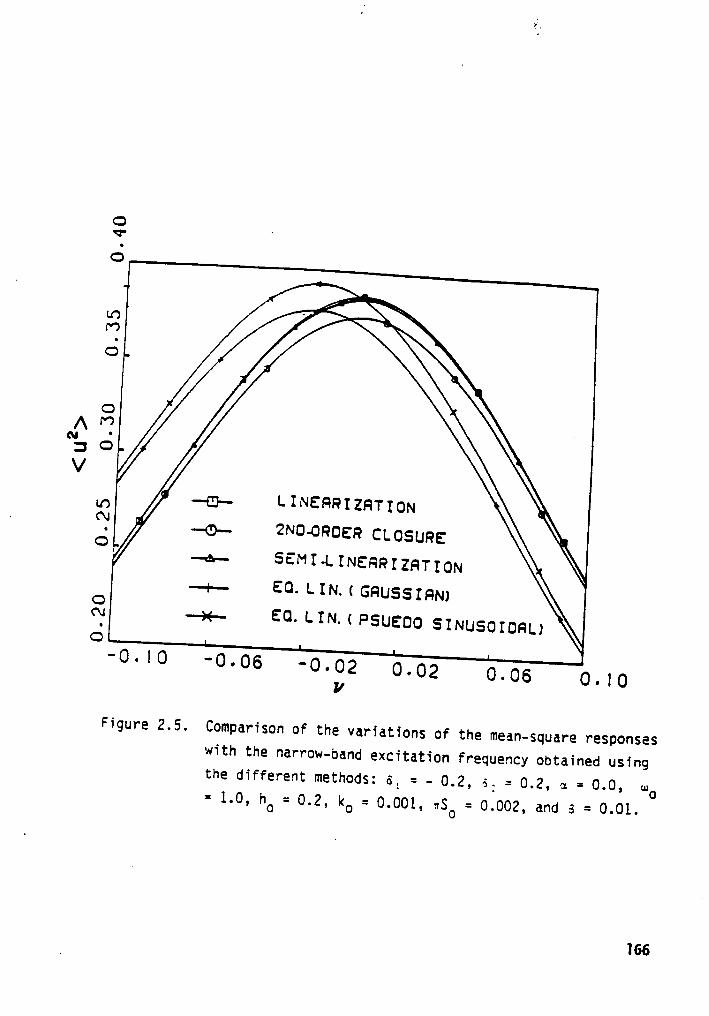
¤ .sr

Q

M

O

O

^ "?ev: OV

Ln '-@- LINERRIZHTION .”

°' -0)- 2ND·0RDERCLOSURECJ-6-SEMI-LINERRIZHTION-1-

EO. L IN. ( GHUSSIHN)OEO. LIN. ( PSUED0 SINUSOIDRLJO

-0.10 -0.06 -0.02 0.02 0.06 0.10V

Figure 2.5. Comparison of the variations of the mean—square responseswith the narrow-band excitation frequency obtained usingthe different methods: 6, = — 0.2, 6. = 0.2, ¤ = 0.0, :::0= 1.0, ho = 0.2, ko = 0.001, ::50 = 0.002, and s = 0.01.

]66

LO

CDC?" ··

— (D 2ND-ORDER CLOSURE „~^ Q

ü3

GIV LO

Q Ü6 =•°0

2 anO

· S c 6_~

2--0.10 -0.06 -0.02 0.02 0.06 0.101/

]67

·¤·

^ .. an _3 N

\/

Q .‘O~¥O·0;06 -0.02 0.02 0.06 0,10

V

STHBLE

· <r

/\ev3 N

. V

O

-0.i0 -0.06 -0.02 0.02 0.06 0.I0V

1 STRBLE

Figure 2.6. Frequency-response curves for 62 = 0.2, 62 = 0.2, ¤ = 0.0,wo = 1.0, ho = 0.3, ko = 0.001, ¤SO = 0.0001, and B = 0.01:a) no noise; b) with noise.

168

-

Q

QI

F7O

A · .cu-

QUV .

OO

O · · -0-03 0-09 0-16 0.22 0.29 0.35 0.42

h° i

Figure 2.7. Effect of the mean amplitude of excitation upon the mean—

square response to white noise For 6,·

0.02, 6;·

0.08,a = 0.05, oo = 1.0, ku = 0.0, w30 = 0.005, and 0 = 0.03.

]69

w (vl) ’Ce /\ /,*\ y1\_ y' ‘!/ '· ‘ x -‘ x 1/ 1/ fl

= {= ' x J

‘. ’ 1 I · ' ! H . 7C } f @ *·’

°- · 2i,

J‘ „ \‘

i. ¤ I J „ F . I . 1 1: ¥ ! · . 1 ; s I ¥ { \ * · . aä

= L I‘. _” r F E = * ; \ J s I

‘* =* ·

’, _ „ _ ; · g‘ ; 3 Ä; ;

„ . x . , · I· } \ 1 Z f \!1

‘Z = 2 : ¤ l z

’3 ·

‘|x [ X „ ‘

*2 vv‘_ .’ i /' n .j ‘l

¤ 7 -,·’ \/ ‘» ‘ »

1 ·v « J 1 ‘. 1 J ‘J

{ al =JI jf

E/\, fl

an . 1 ,\ [ [ ¤ · v

\ 1 \ ] x \ V 7 EG \‘

\ I * ; * ' { ‘ · · ;· .

·r ! a ; R : ä * 1 ¤

*5* L / \ ! 2_ ; ‘; \ [ \ 1 * E ä

·- ¤ f x J x I ; 3 ·\ , X E :=· - „ : „ \ EE • r Ä ' *, ‘?

I / \ [ x x w I x 1 I‘ I a ‘ ‘ ·* I — I x z

‘/ ‘\/ ·‘

c> „ ‘ \ _!\ I‘\ ; a g

Q ; \ l \ i• I Ic ' I Y Z - \il

‘1 71 ;

: g\ I'é / \ 1 ‘

‘?[ . . ~J . Q 1750 758 767 775 783 792 8GC

X

Figure 3.l. Ccmparisan of che timamistcry respcnsa for orimary

resananca predäctad by the mechcd of e·:ui·:a?en:

Hnaarizatfcn with chcsa cbtainsd by the method cf

avaraging and numarical simulation Fcr ua = LO, u =G.O7, 1 = 0.2, F = 0.l, 1; = 0.Gl, and a = L3: (a)a*:u‘v·1'a¤: '€near·‘:acf:n: (:1 avaragingz an: {·:‘ v·ur‘2*‘:1'

s‘rnu'ac€:-1.

'I70

C1 ,/\ 2; ,/ j»·~

[Ü ’/\ \‘ ‘

* ¤ / Ü1 1 //—1._ Li i ’ \L|Ü

/‘\ II \\ / Iz ‘._ /’ ‘\

1Z, 1, /1 x_ / 1\\ ',L‘ '

w 1b1"i

/xa-\ /\,.\L :’

' x EG I 1/ ’. L L 1 / / -. ;O { =L !

‘\¤_;t \ ‘.· 1 1

” 11 \ '

O_ X/Q LI ·

__ _ Ü

: (C) ··°I—Ic \ 1„ \\IÜ?

/ I!11I\c

750 758 757 775 783 792 800X

Figure 3.2. Icmpariscn cF zre time—his::ry reszcnse Fer sucernamcnicrescnance cf ·J?'ZE’-ZTIT?.2 sredictez ay the 16:::: cfecuivaierrt iinearizacicn .«i:h those :¤:a‘n6: by the 16::::cf averaging anc numericai simuiatfcn for :1L_ = 2..0, : =2.02, 6 = :.2, F · 0.6, 1L = :.:2, and 6 - ;.:: (6)ecuivaienz iineerizaticnz Ib) avereging; anc Q:) numee-‘:eisimifaticn.

'|71

x I(1_! ·'

c ....------—--———--———---..................____I 2I II ·

*5 I I',\ /\ v.\‘ \

‘ \ "‘ ‘

1

‘ ‘_l '\ /\ .,1 [Q ’\

[A \/,Q

I1% ‘

V‘

'~ 1

Ä1 V IJ .. .

‘-.1 « « «· « I/

‘· ‘J V' ‘.1 ki V VI '·./ ‘.·, ‘·,,'

IéI . ·lE

II II ‘. ‘— II "” I

1 / . I 3 ' I ·_ .¢ I I~ I _~ I~ ]~ 1

I”I

¤”=

/”· 4 I

6 I ;'‘ ‘ I

‘= E I 1

‘- · i

I ; I E I I · · { I Ü 2 I I· ' I , I I I

Q I · ;_I I j E I ‘ I ' I II . I ' I

I I 2 I 2 2 I E I I_ ! I I j I„_ \IJ °J IJ ‘J Ii II '·J ”

l .

&. (C) .Q .

\·, I \ 1 _!¤ I V I I I<= I I I· I I I 1 =\ I I

I IIf

I‘ I ·ca I

75C 755 757 775 753 752 SGSBC

Figure 3.3. Comoerfscn of the :Ime—his::ry response For supnermcnic

resonance of order one-third pred*c:ec by che nechcc cfecuIva1en: Iineerizezicn wIth those cbtained by the hechodof everaqing anc humerice? simuiatfcn For JO

-1.0. :

·GAL, 6

·0.5, 5 = l.25,~1,

-0.15, en: 6

·1.2: (e)

e:u‘va‘en: TI:eer‘:e:€cn; (5) avere;‘n;; anc (ci numer€:e2simnüetion.

]72

Q U Q U cQ III U I~ cB II ll •I3

° °•¤ 14-:„ " ·=>° U- «—•>,

I QI •r-Q) •@I 14-1n •-amI 14-eu 4-:I ::0 11U

' QUQQSI¤.I.:••-mw

: 1 .:4-: s.I

• J-I CUB-I c LOCI U-O••·I¤II Qu-4-: 1I

•¤•1

IIn

äßäaäe'FI Ü $25114-·°U

”°LIUO gd-I

{ ° „?6E’°°¤SI L¤.•¤•¤J·•·I •¤ xmms.

· { ääucäääI OC

Ida-IIU_ I , IDG)! UH

wwtgugI ä .6·=·s·>~··=I

4-: ca:Q-CUl|'Q3

{ °°”E:„23I ws- UI •I UOg•·••-u.I . :4-:s.o¤QI

°

1U¢¤¢¤•t‘DI ‘¤•··.:•-•$-'QI CPL ¤.OI dJ·¤··GJII SI ¤.U¤. 4-:I QJMIIOIQJI QOVIB EI

' .{ 9 <#¤

•·-1Q U Q II QQ GI II BQI~

II ll ••Q

=I I I I I ciQ Q Q Q Q ···—

x Ln

l73

66r~U

6S

6

l

U

6n CI

Q

·6

6

Q6•¤u.

lé-I

•

cwO

-'

E°’?2>~

I

:3}

O‘°

I

'·¤

2

66 M3

•

w¥—"u

I

mg

2

··-äävä„.:

222

3:62--

·

nmlääawü

•,a1g

G2.

I

o"o

ws.

m„_

4-I

I

!U_·QI¤

I

„=¤,LmQN

g

•¤•¤'c

mv-

}

‘1‘};€cSg_ä

.

C=•¤OW

2

"*‘62‘2"2·6

2

°E‘=ä°.„’°

GJ

;•u

I

ga)

(*1;:

I

4:*-

6-•

•

‘“‘e-»'gq E

I

M-

Ogg

I

Oguu>

°•-

'•-

I

GJ:

U:

2I 6

GJ"°E•U

I6

S66

n2

6,,;

E

<j.g

2°”

z>

°

E

0

=6 E

kk

I74

Q II Q II 9Q N I! I~ 9B D 0

••9

Q Q Q Q 9 ¤ ..2I °

•¤ •4.»• Q‘,

Z 2*¤ :=I

·•·¤) Q?I U-vl •q)

I•+-ru •-·•-•-Z

I su; oI Q QQEIIZE•

’ |• Q)-C Öu)

·¤

.‘ä“„;‘^ZaF ..6¤2.{ Qu-6-»«¤¤

'u>B

I

'VI

-1-•-:•

'cs.u¤·o

I ou><c>o·: "Z azwésäI Ö IDEE

•D·v··• Lmousu• LU •¤

I·•·

' ZL"äS°°B'“'g · >«¤ x„•·ms.| SCI MOM

¤‘:·¤ au{ ¢^···¤C;oc

ICIU Lv-

·I‘

'

¢¤+-••I Q uuxcuu• E°€«Jf$I uuno ·—I .c.:«¤•>,•¤

:+->«•-•Cc.¤>

1} •• °°°E BE• uno uI UOE•·•·¤-• äZa’?6°'ä°: ‘¤•-.C-•L7

'

Cr—L CLÖ

'

¤J·•··¤)II .C

' ¤.U¤. 4.•·

umso u

'CGI/*3 E

V QI . .

Q RD

Q ll S II Q· 'o tu

•~ o‘”"

B D UI * Ö q;O O l O t L

Q Q Q Q Q 3ov

(ZX) II

175

1.00 _ 1.00

0.75 0.75

A‘“',_,¤.s0 0.50 e

- V ·

o.2s ___,-----*"°'°°‘ mas

0.00 0.00

0.0 0.4 0.I 1.2 1.I 2.0

-4S0XFigure3.7. Variation of the mean-square response of the Duffing

oscillator with the spectrai ampiitude Sc of asuperharmonic narrow—band random excitation for,mo -1.0, u = 0.03, a • 0.3, s = 0.001, and v = 0.25: __predicted by the proposed method; —-- predicted by themethod of equivalent linearization.

176

S,. -~

w

I Sfx

IS. I

I

I—I—

{C!) .

(DO

Figure 3.8. Spectral densities of F, fl, and F,.

177

15

12

s‘s

^

‘s

es °~,

·

~§

V0

‘0.00 0.05 0.10 0.15 0.20 0.25

ld

Figure 3.9. Variation of the mean-square response of the Duffing

oscillator with the nonlinear parameter a For the case of a

white noise, eo = 1.0, u = 0.03, and SO = 0.3: ___ exact

solution; ——- eguivalent linearization solution; and o

proposed method._

178

15

12

/\ X,Öl B

‘s

*<‘

1————

0

0.00 0.05 0.10 0.15 0.20 0.25I

Z5

Figure 3.10. Variation of the mean-square response of the Van der Pol-

Rayleigh oscillator with the nonlinear parameter Y For the

case of a white noise, oo = 1.0, u = 0.03, and So =

0.03: ___ exact solution; --- equivalent linearization

solution; and o proposed method.

179

ID O IO Qg N ID N O{ m m M •—

=> 5 „ 3I I I I I I 9 I I I I I l I I I I I 'I• CV Q\\

^^ I ud 1 G‘

ea 1\ N_:*1 • IIÜ — ~• I ÖlÜ‘ bV

[ • Q,s ' V ‘ G\ I GA s\ I II.„

=

‘\

I: c 1 •°

v * • ‘°\

I 11 LÜI O III 14.s I N‘g

* I Int 9s'

GJ\ I >Ü\ I g •~„ 2 ¤ 3 °s\ I IIs g ,.„

NyI

^

‘£<

9\\

I N•~ •

\ I VI In 0)s\ I Ä ID , ,.‘I L Ö «¤s I V 1 eus I N cu II id\ In U en’ Nx I • L N c

~\ 1 o .2‘

=\ I •

II s I m 1.n 1I

"I > N I

! Ns I ·•-¤ O ~••1 \ I G C)I Ü\ I In 4-P II P-‘

I I C .¤‘I.- N G)

" GI \ {I 5 3 < Ü

X IIE-

U;IG

1 = <rQ cuID Q ID O8 r~ In cu Q ä

Id In Q] FI C L';

180

5-¤¤ ‘——__——‘"_””____”—”“—"__””‘"'‘''—"“m“°”'”"”‘”'""5.00

2< (I2 >„·’°„·'3.75 „„· 3.75. ,,0

„·"

2.50 ,·’2.50

„·"0

„·",0

0 .

fz'1.25_,»’ ‘ 1.25

„·",0

2<1ag >0 , 00

•------·~-··-·······•··•····••-•-•-—••--••-·-· 0 , 00

0.00 0.26 0.52 0.78 1.04 1.30‘2

< F >

Figure 4.2. Representative force—res¤onse curves for ul = 0.2, ut =0.5, Al = 0.25, A2 = 0.5, and 6 = 0.2: ___ stable; ---unstable.

181l

c III c¤ r~ nn lg 3so m cu •-I 3 c

' ° n •z A•·•

öl:-TÄ-

1 {I' ( Omc V |IV2

I_§ 9 *=' 1; · n •I

^:

-• <r2 **:1

gc

I N =• sö uV | u. NS \ 2 „

I ? A goI { hl w uz | ‘

..2 g ;* 22;! • V Ei • .2 ä ,*5* $9 *2E . I'___ I ¤ é,. 132 L

: L wgg, c < EZ °

"‘ ,I [ QJRDIä Q

· an .Z"Z'§ ‘-I_N

ug ••r•\IQ 4-* II P

s I 5 -€2 I V! <d-9

2 I I, S26 I[ _,¤

o an c an é ° "Zo r~ ID tu o QD N N ~·• _Q„

3LL.

182

2‘ _

° Q) ••

. N .c LD5 ·e-• 0 1:\ Q 0 C\‘ Q- • I5

‘ A o 0OA \\ N:4 vg u

.

A g \—

O -·V ••- 1lIN-: V \ Q JJ=

"

N Q g, N

V‘ • C OI?5‘ ' Q ,2 °" ,\ C 0‘ en O ·5 I5 ”" Ö‘ A-I‘ Ih I'5 l'

5 g·*-‘

> cu‘\ •• F7 3 ‘,{‘ ,.5 6 I ··- zu U; g‘ ;

5 $ ¤. u N ee5 E „- „ gn5 "'* eu •-» 0 C5‘ vv I :‘

.I •

‘ ‘c

••• Nlul o E < ¤

O O~ " J 3 ä -"

6 ä q,) u LD IDL ID • I-• ‘¤ 0 .¤‘ cu I5 _‘ ä n e;

5\= JJ __‘ 3... < |‘

U5 u O5°

C sr;\ · I5 U O ••

Q ev ·: 0 0E Q •

u 0 uI5 •— II A‘¤ ¤. ~O E ju-

cZ ru

- v

°.

¤ <rD Q D Q ·S r~ D N o <"

•·• Q Q Q Q L:c~I ‘* ·X (ZU) C

183

7

.

<"—a2>Xl03

8 an_; 'Trn c

E ° 6 =>o c

1

5SSE

?

Ce:

.

‘¢5•Ä c.

äN^

gnq

ä "

G

5 _ __^ g, fi,.

x

I· ¤o«>

sV [° 2**-

V1

L$25;

Q

LV $$3"·-·

LV¤'° E'-

-ä’

"‘ §·¤~:

ELL

•-• c°E Nä

‘·LSA- äE<·-·

;

f'. $¤u."’

¤

"ÖÄZ

gv J']

'

ag ,¤U7•—•

I• wvc.

·

T° "’On

¤L SIZ

EL

gérll,/\

8 nn oLo .

.|\

uw

I

Q

G ' . o "

° ° 5 23

184

IO• QN

„ In

~·~

I

‘ ·*“I C,

I

¤.

IE

xI

‘? C,__ ev

I

‘~ Ici 5

A XI

Q

N‘\s

?

IS

¤X

ILIn

__II

V\

„L : N A

.X

o °^·

~I I' EYS O K7

•- UL

g Il E

I I"* Ä '°

A

I

„, L,

NNI

°° O Ü

°"•·•••-,_V

*¤ "

••·---,______________„ I E

3< > II •

änII

I

°~

VI Q

I

‘—~‘

II I•*• ¤.

I

‘ „ V C:6 E

*“ ‘

1

:

I

I IIT Z I5 J

\ Tep "'°

• E

\ L

g,w

•-•

\ I

6U 3

I

I .. ä U II In

I *-' *1* T s

' Q Ü I:"’ I

I '¤¤ Q

•

I! -O

Q II, N,_

II I

E L$2

I, I.I—

I

1, •IZgIII*8

_I_, II X

N

ll·

Zg N

•—•

·¤¤

IL 6

·¤ „ ·

.: **2I, 6 ~=z

O. I

<r

.

°

euI-:E’

Ln

185

O . B g _ g

••-•---O---••---~•„_’••---•••·••--Ü-•-•••·

‘~ [Ü‘s‘ Il,

~~~• ,,/A

° ·‘ G 0 . 4

A A*1 ** soV V

¤ - 2 / 0 .2

¤ - ¤ · 0 .0· -0.2 -0.1 0.0 0.1 0.2

V

Figure 5.1. Dependence of the mean-square responses on the detuning

parameter 0 for the case of a two-tc—one autoparametric

resonance, 0, = 0.5, al = 0.02, el = 0.03, S; = 0.0,

S; = 0.01, S12 = 0.0, al = 0.1, anc 6, = 0.08: ————

<x;> and —-—- <x:> predicted by the non—Gaussian closuresoiution; o predicted by the reduced non-Gaussian ciosure

sc1ution.

186

4 4

ll

3 // 3I'I

„·'./9

/\ · x" _^ew ..

„„·’ we

NV„·"é1 1

„·"" ',¤"' ‘

I

0 ' g 00.0000 0.0233 tgz 0.0dBS 0.089S

Figure 5.2. Variation of the mean-square responses with the excitation

spectral amplitude SZ for the case of a two—to-one autopara

—metric resonance, 01 = 0.5, 02 = 1.0, 1, = 0.02, 02 =0.03, S, = 0.0, S12 = 0.0, ai = 0.1, and 62 = 0.08: ———-

<xi> and -—-— <x;> predicted by the non-Gaussian closuresolution; o predicted by the reduced non-Gaussian closure

solution.

187

0.a_

°B

X ,\\

X‘\

°'s °~._ 0.5

A· A

N 1

N °"0.4 Ze

vN

~V

0.0 aß

°

‘°· 1¤¤ 180 240 soot

Figure 5.3. Time history cf the mean—square responses predicted by

using the Gaussian clcsure scheme For the case of a two-to-

one autoparametric resonance, 0, = 0.5, dz = 1.0, v =

0.0, a. = 0.02,;.; = 0.03, S, = 0.0, SZ = 0.01, S1, = 0.0,1 7

al = 0.1, and 6: = 0.08: —— <x;>; —--- <x;>.

188

0.8 ,0.8

‘I

•‘s

I

°s‘•

0.6‘,, ‘ 0.6

A AN 1

•

H 0.4 0.4,jN

VV

0.2 \ /_ 0.2

0.0 0.0

0 60 120 160 240 300~ t

Figure 5.4. Time history of the mean-square responses predicted by

using the non-Gaussian ciosure scheme for the case of a

two—to-one autoparametric resonance, u, = 0.5, mz = 1.0, v

= 0.0, u, = 0.02, u2 = 0.03, S, = 0.0, S, = 0.01,

S,, = 0.0, ¤, = 0.1, and 6, = 0.08: —— <x?>; ---— <x,>.

189

1.00* 1.000.75 0.75

,

N Ä^H o.so 0.:oNJV . . V

A Älijl 7 °:Ü?:IYi 1 ?ÄZÄ€Ä?‘€:E7;i»f?€i 1 iiiT•-•=:ÖjTY‘j·Ä·ÜÜ‘ T IjÜ—Z~·I—j·Z—Z· ~I I·I:·Z·I·L;‘·I

‘ .§-Z:y6:g:—'4— "\ ' ' * ‘ } n • q- T

s0.00 ·······•···• . 0.00. A ‘ A ‘ A ‘

0 400 ECO 1200 1E0O_ 2000

Figure 5.5. Time history of the mea.n—square resconses preoicted by

using the Gaussian ciosure scneme for the case of a two-to-

one autoparametric resonance, ~« = 0, ul = 0.03, -4; = 0.02,

66 = A:. = A16 = 0.05:-190

1.2

0.9

^- /\

... Pe

, V\/ .

O . 3 ~·°°‘~·.,___

Ä °'“°"‘•··e·——-I

0.0 Z

-0.40 -0.24 -0.08 0.08 0.24- 0.40V

Figure 5.6. Uependence of the mean—square response of a shaiiow arch on

the autoparametric detuning parameter 0, ul = 1.0,

ul = 0.08, bz = 0.05, S1= 0.05, S, = 0.0313, Sl, = 0, and e1 =

0._1:—— <x;> and -——— <x;> predicted by using the”

exact stationary soiution of the FPK equation; 0 predicted

by using the non-Gaussian ciosure solution.

/‘

191

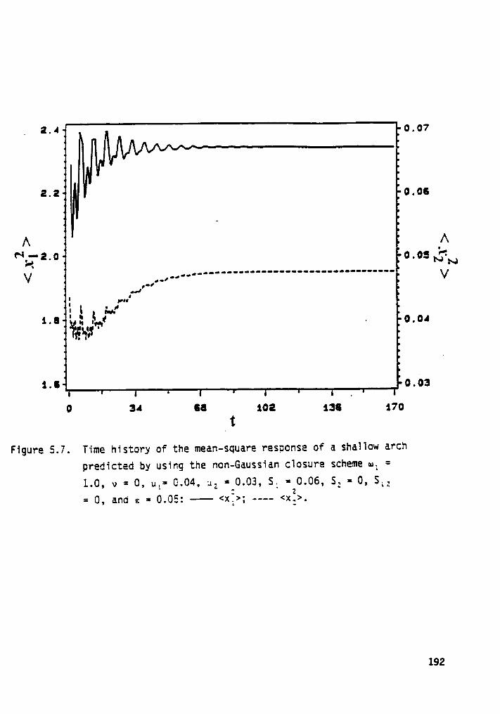
. 2.4 0.07

2.2 L 0.06

/\ /\***2.0 g gs F1

H

• e

‘~l_"‘·—QQiQQC¢¢¢¢¢¢¢¢¢¢¢¢¢¢¢_¢¢¢Q¢Q¢¢Q1;:

‘Jon,

¤ ie.La · R sv} - 0.04¥,;>,:¢·

1-9 0.oa

0 34 68 102 138 170.t

Figure 5.7. Time history of the mean-square response of a shailow arch

predicted by using the non-Gaussian closure scheme o. =

1.0, v = 0, u.= 0.04, dz = 0.03, S. = 0.06, S. = 0, S1.= 0, and E = 0.05: ——- <x.>; —--- <x;>.

192

2.30 0.100

·^N-2.23 ; w 0.030 H‘s‘ , NN

V .· ‘. V.‘”°~

; \a \

of,"\

ag~‘•‘··

‘\

2.00 0.000

-0.37 -0.23 -0.12 0.00 0.13 0.23

V

Figure 5.8. Variation of the mean—square response of a shallow arch

with the autoparametric detuning parameter 0, u, = 1.0,

ul = 0.04, ug = 0.03, S, = 0.06, S, = 0, S,, = 0,Z · -2

-_

and a = 0.05: —-—— <x,> and -——— <x2> predicted by using

the non—Gaussian closure solution; o predicted by using the

reduced non-Gaussian closure solution.

193

2.00

1.25*

.A‘~._

.^L, 1.°70

1- 4 s~ ' FJvU U V¥r·~_

1.55 °~s~‘2

eßs‘sss

~sq‘ss‘~

1.aoII I I I I I I • • • I I I ‘ I I • I I I I I ‘ I I I • • I I I •

·-0.2 -0.1 -0.0 0.1 0.2

V

Figure 5.9. Comparison of the variation of the mean·square responseswith the detuning parameter v for the case of a one-to—oneautoparametric resonance. Results are obtained by usingd‘1l:f€Y‘€!!1°. mEÜhCdS ?OY' U2 = 1.0, L12 = 0.02, L1., = 0.0].,

S2 = 0.04, S2 = 0.02, S22 = 0, 322 = 0.14, 3,,2 = 0.].6,an = 0.15, anc a2, = 0.15: <x;> exact solution;··—· <X2> EXäCZ $OlU'ClOI’1; O f‘ICf'I—GöUSS1d|‘l closure SCUIUCÜOI'1;

+ reouced non—Gaussian clcsure solution.

194

0.5·

O.4A

_ AN; 0.: i ,5N

V *2* V\“‘\—•\•‘

0.e °°"*···········—···········—·—-·····—··—----

O.:l

0 • I I I l I I n • •I n • • ‘ • n I

0 50 :20 :00 240 300

t

Figure 5.10. Time history of the mean—square responses For the case of a

one—to-one autoparametric resonance predicted by the non-

Gaussian closure scheme For 112 = 1.0, 0 = 0.0,

112 = 0.03,112 = 0.02, S2 = 0.0]., S2 = 0.0, S22 = 0.0, andBil = Biz = 0.05: —— <x;>; ·——— <x;>.

195

0.55 0.24

IlqgI, ‘y

0.50 j x0.18

ll \‘ A’ •'° s

A "°·

9],-,°

‘· ,1 • P\7

. .. /1 i 0.12". V

sf ·.ll

‘

0 \ln, ‘\

0.40 -·‘··‘r,»" ¤‘‘ 0.06

§§~—&-·-

0.35 0.00

-0.40 -0.24 -0.08 0.08 0.24 0.40”V

Figure 5.11. Dependence of the mean—square responses predicted by using

the non-Gaussian and reduced non—Gaussian closure schemes

for U16 CESE of 6. 0|1€·tO-CHE dUtODd.l"ü.mEU'1C TESOHQHCS OI1

the detuning parameter u when ui = 1.0, ui = 0.03, ug =

0.02, Si = 0.01, SZ = 0.0, Si: = 0.0, and Bi, = Biz =

0.05: <xi>; ——-- <x;>; o reduced non—Gaussian closure

solution.

196

2.0··

\—‘——

2.5‘~,

^ >‘\~

"l1..

1.o0.5.

0.0 '- I

-0.40 -0.24 -0.08 V 0.08 0.24 0.40

Figure 5.12. Dependence of the mean-square response of a string on the

autoparametric detuning parameter u, ul = 1.0, S, = 0.03,

SZ = 0.03, S12 == 0, uk = 0.03, 12 = 0.03, and E = 0.].:z—- <x.> and ---— <x2> predicted by using the exact

stationary solution of the FPK equation; o predicted by °

using the non-Gaussian closure solution.

197

2-9ä 2.03i.5· Lg

N/\ in AQ1.oV

v

Oßä o.:nä

\~•••—·I

¤-¤ ''''°‘'‘‘••••••······················· 0.0‘ I I

0 B0 160 t 240 S29 400

Figure 5.13. Time history of the mean-square response of a string

preoicted by using the non-Gaussian ciosure scheme, ul

= 1.0, -1 = 0, S, == 0.03, S2 = 0, SL: = O, =

0.03, ::= 0.03 and T = 0.1: -—- <x:>; ·-—- <x;>.

198

2.0] 2.0

ä1.53 . 1.5

^A

N; °

E 1..o 1.o gwV V

0.5- e 0.5•

I

0.0l

0.0I

• 1

0 80 150 240 320 400t

Figure 5.14. Time history of the mean—square response of a string

predicted by using the non-Gaussian ciosure scheme, ul

=1.0, v = 0, S1 = 0.03, S2 = 0, S,2 = 0, u. = 0.02,2 z'

p; = 0.02, and r = 0.1:- <x,>; ———- <x,>.

199

2.0-1 tag

1.5g_5

.„^ ^;' 1-¤ 1.0 Ev° NNV

¤-5 0.:

¤-0 0.0I I

0 ao aso 240 220 400I

Figure 5.15. Time history of the mean-square response of a string

predicted by using the non-Gaussian ciosure scheme, 0.

= 1.0, v = 0, S, = 0.06, S2 = 0, S12 = 0, ui = 0.03,

dz = 0.03, and r = 0.1: —— <x;>; —--— <x;>.

200

' 2.A§

1.8-%

° A^ 2

s}

" v

0.6__„•*’”

0.0 —·——-e-·—·-······--•-··"”I

0.00 0.02 0.04 0.06 0.06 0.10$1Figure 5.16. Variation of the mean-square response of a string with the

excitation spectral amplitude Sl, ai, = 1.0, v = 0, SZ = 0.S12 = 0, ul = 0.03, 02 = 0.03,- and I = 0.1:——— <x;> and --—— <x;> predicted by using the non-Gaussian

closure solution; o predicted by using the reduced non-

Gaussian closure solution.

201

2.4

L?.1.2]AV

ßv

0.5,'·’

"~„ .1

\_III s~~

I .

~l‘~„

0 . 0·I’e

-0.05 0.05 0.15 V 0.2 0.2 0.45

Figure 5.17. Dependence of the mean-square response of a string on the

autoparametric detuning parameter v, ul = 1.0, S, = 0.07,

S; = 0, S., = O, ul = 0.03, u. = 0.03, and E = 0.1:: " 2 ' .-——— <x;> and ---- <x,> predicted by using the non-Gaussian

closure solution; o predicted by using the reduced non-

Gaussian closure solution.

202

2.0‘

1.5

A";: 1.0 - Q}v' "'”~

V

0.5

""*‘P'•••· -—•••---,

____t qp —·°

‘P"°'•<Q•-••••*•••1

0.0

-0.2 -0.1 -0.0 0.1 0.2

V

Figure 5.18. Comparison of the variation of the mean-souare resoonses

with the detuning parameter u for the case of a tnree—to-

one autoparametric resonance. Results are obtained by

using different methods for u; = 1.0, ul = 0.02, o; = 0.01,

S; = 0.04, S; = 0.02, 5;; = 0, 3;; = 0.14, s„; = 0.16,

a;; = 0.15, and az; = 0.15:-- <xZ> exact solution; -——-

<x;> exact solution; o non-Gaussian closure solution; +

reduced non—Gaussian closure solution.

203

z"° o.o4:‘l

?•„ _II°•

2.05 1 ,LUH 0.022

/\ X '^N1.70Vs

"‘‘\‘\

.‘,_ 0.02:1.::

‘—,

1.oo , _ “·°·°°°°°°° 0.0120 80 $.20 $.80 240 300

t

Figure 5.19. Time history of the mean—square responses predicted by

using the non—Gaussian c1osure scheme For the case of a

three—to-one autoparametric resonance, ol =1.0,

v = 0.0, ul = 0.0]., 62 = 0.0]., S, = 0.02, S2 = 0.0, SL:

= 0.0, and 6,, = 6,2 = 0.05: —— <xi>; ---- <x;>.

204

2 . 50 0 . 0220

S

2. 45 Q Ü .°2s5

A•ea

'I —^;'e.4o ,'

‘.0.011o Fe• In N3 ggV v1, ‘

I, s‘ „,1 s‘

2. 35 "/T! \‘ 0.0055

§——F_—__

2.30 0 .0000

-0.40 -0.24 -0.08 0.08 0.24 0.40V

Figure 5.20. Dependence of the mean-square responses predicted by using

the non-Gaussian and reduced non-Gaussian c1osure schemesfor the case of a three-to—one autoparametric resonance on

the detuning parameter 0 when el =·1.0, u,= 0.01, ug =

0.01, S; = 0.02, SZ = 0.0, SL, = 0.0, and eiz = 0.05: ————

; —- · ; O T‘2dUC2d ¤O¤—GdUSS1dV1 CQIOSUTE

so1ution.

205

5.00

3.75

A _ /\N .. R

pg 2.50 Nw

V V

1.25

‘‘‘'''0.00-··"‘

0.00 0.06 _ 0.12 0.16 0.24 0.50S1

Figure 5.21. Dependence of the mean-square response of a hinged—clamped

beam on the excitation spectral amplitude Sl, 0, = 1.0, di

=°·°‘*·

=: = °·°?· v = 0-ZM S.; =0——<x;> and ---- <xQ> predicted by using the exact

stationary solution of the FPK equation; o predicted by

using tne non-Gaussian closure solution.

206

5_q 0.04

4_5e 0.03

6A · /\**:.7

3_¤ _ 0.02 QNV V

1.:_,g"”

0.01

teefféß .°_° -··‘ 0.000.00 0.07 0.14 J; 0.21 0.28 0.38

1Figure 5.22. Variation of the mean-square resoonse of a hinged—clam0ed

beam with the excitation spectral amplitude S2,v = 0.21, ui = 0.04, ug = 0.02, S2 = 0 and S12 = 0:2 2—— <x1> and -·—- <xZ> predicted by using the non-Gaussian closure solution; 0 predicted by using the reducedn0n—Gaussian closure solution. .

207