Embed Size (px)
Citation preview

I N S T I T U T D E
S T A T I S T I Q U E
UNIVERSITE CATHOLIQUE DE LOUVAIN
D I S C U S S I O N
P A P E R
0712
LOCAL LINEAR QUANTILE REGRESSION
WITH DEPENDENT CENSORED DATA
EL GHOUCH, A. and I. VAN KEILEGOM
This file can be downloaded fromhttp://www.stat.ucl.ac.be/ISpub

Local linear quantile regression
with dependent censored data
Anouar El Ghouch1
Institute of Statistics
Universite catholique de Louvain
Ingrid Van Keilegom1
Institute of Statistics
Universite catholique de Louvain
July 16, 2007
Abstract
It is known from the literature that the least squares regression estimator is
optimal and is equivalent to the maximum likelihood estimator when the errors
follow a normal distribution. However, in many non-Gaussian situations they
are far from being optimal. This is especially the case when the data involve
asymmetric distributions as is the case, in general, with survival times. Another
known drawback of the least squares method is its extreme sensitivity to mod-
est amounts of outlier contamination. An attractive alternative to the classical
regression approach based on the quadratic loss function is the use of the abso-
lute error criterion, which leads to the well known median regression function,
or more generally, to the quantile regression function.
In this paper, we consider the problem of nonparametrically estimating the
conditional quantile function from censored dependent data. The method pro-
posed here is based on a local linear fit using the check function approach. The
asymptotic properties of the proposed estimator are established. Since the es-
timator is defined as a solution of a minimization problem, we also propose a
numerical algorithm. We investigate the performance of the estimator for small
samples through a simulation study, and we also discuss the optimal choice of
the bandwidth parameters.
KEY WORDS: Censoring, kernel smoothing, local linear smoothing, mixing se-
quences, nonparametric regression, quantile regression, strong mixing, survival analy-
sis.
1 Financial support from the IAP research network nr. P6/03 of the Belgian government
(Belgian Science Policy) is gratefully acknowledged.
1

1 Introduction
Quantile regression (QR) is a common way to investigate the possible relationships
between a covariate X and a response variable Y . Unlike the mean regression method
which relies only on the central tendency of the data, the quantile regression approach
allows the analyst to estimate the functional dependence between variables for all por-
tions of the conditional distribution of the response variable. In other words, quantile
regression extends the framework of estimating only the behavior of the central part of
a cloud of data points onto all parts of the conditional distribution. In that sense QR
provides a more complete view of relationships between the variables of interest. Since
it was introduced by Koenker and Bassett (1978) as a robust (to outliers) and flexible
(to error distribution) linear regression method based on minimizing asymmetrically
weighted absolute residuals, QR has received considerable interest in the literature
both in theoretical and applied statistics.
In survival (duration for economists) analysis, QR becomes attractive as an alter-
native to popular regression techniques like Cox proportional hazards model or the
accelerated failure time model; see Koenker and Bilias (2001) and Koenker and Geling
(2001). This is potentially due to the transformation equivalence of the quantile op-
erator; see Powell (1986). Thus, one can use any monotone transformation of the
response variable to estimate the QR curve and then back transform the estimates to
the original scale without any loss of information. For a review of recent investigation
and development involving QR see for example Yu et al. (2003) or for a more detailed
lecture see the book by Koenker (2005).
A frequent problem that appears in practical survival data analysis is censoring,
which may be due to different causes. For example, in econometrics censoring can be
due to the loss of some subjects under study, in clinical trials censoring can be caused
by the end of the follow-up period, in ecology or environmental studies, a single or
multiple detection limits lead to censored observations. In recent years parametric
and semiparametric quantile regression with fixed (type I censoring, namely the Tobit
model) or random censoring begun to receive more attention. See for example Cher-
nozhukov and Hong (2002), Bang and Tsiatis (2002), Honore et al. (2002), Portnoy
(2003) and the references given therein.
As an alternative to restrictions imposed by (semi)-parametric estimators, a vast
literature has also been devoted to the nonparametric QR method. With completely
observed data, this includes Fan et al. (1994), Yu and Jones (1998), Cai (2002), Gan-
noun et al. (2003) among many others. However, under random censoring, the available
studies are fewer. Let’s first review some recent work that has been done in this area.
To estimate the conditional quantile function, Dabrowska (1992) and Van Keilegom
and Veraverbeke (1998), among others, follow the classical approach of inversing the
conditional survival function estimator. The latter was obtained by smoothing with
respect to the covariate using either Nadaraya-Watson or Gasser-Muller type weights.
Strong asymptotic representations and asymptotic normality has been shown. Follow-
2
ing the same idea, Leconte et al. (2002) proposes to estimate the conditional survival
curve, and so, by inversion, the quantile function, via a double smoothing technique
using Nadaraya-Watson type weights. That is, the resulting estimator is smooth with
respect to both the response variable and the covariate. Gannoun et al. (2005) sug-
gested another approach based on minimizing a weighted integral of the check function
(see (2.1) below) over the joint distribution function estimator of Stute (2005). Under
strong assumptions on the data generating procedure, they prove the consistency and
the asymptotic normality of the proposed estimator.
The literature mentioned above focuses on the i.i.d. case. However in many real
applications the data are collected sequentially in time or space and so the assumption
of independence in such case does not hold. Here we only give some typical examples
from the literature involving correlated data which are subject to censoring. In the
clinical trials domain it frequently happens that the patients from the same hospital
have correlated survival times due to unmeasured variables like the quality of the
hospital equipment. An example of such data can be found in Lipsitz and Ibrahim
(2000). Clustering can also be naturally imposed by the experiment like for example
the data analyzed by Yin and Cai (2005) which involve children with inflammation of
the middle ear. Censored correlated data are also a common problem in the domain
of environmental and spatial (geographical) statistics. In fact, due to the process
being used in the data sampling procedure, e.g. the analytical equipment, only the
measurements which exceed some thresholds, for example the method detection limits
or the instrumental detection limits, can be included in the data analysis. Examples
of such data can be found in Alavi and Thavaneswaran (2002), Zhao and Frey (2004)
and Eastoe et al. (2006). Of course many other examples can also be found in other
fields like econometrics, financial statistics, etc.
Another commonly used assumption in the theoretical analysis of censored data
is the independence between the covariate and the censoring variable. This technical
assumption is required to make the estimation of the censoring distribution more easier
(without smoothing). However, this strong assumption is reasonable only when the
censoring is not associated to the characteristic of the individuals under the study; for
example, when censoring is caused by the end of the study.
In this paper we propose a new nonparametric estimation procedure of the quantile
regression curves based on the local linear (LL) smoother. This smoothing method was
chosen for its many attractive properties such as no boundary effect, design adaptation,
and mathematical efficiency; see Fan and Gijbels (1996). In the context of dependent
uncensored data the LL approach was successfully applied to the quantile regression
problem by many authors, see for example Yu and Jones (1998), Honda (2000), Cai
(2002) and Gannoun et al. (2003).
The estimator proposed in this work is shown to be valid even when the censored
data are correlated and when the censoring distribution depends on the explanatory
variable. The proofs provided for consistency and asymptotic normality are stated
under weak conditions. Whenever those conditions are fulfilled, our estimator enjoys
3

similar properties as those of the ‘classical’ LL estimator for uncensored independent
data. Furthermore, to solve the known computational complexity related to the QR es-
timator (like the non-differentiability of the objective function) we adapt the Majorize-
Minimize (MM) algorithm as proposed by Hunter and Lange (2000) to our censored
case. The resulting algorithm is simple to implement and rapidly converges to the
solution.
The paper is organized as follows. In the next section we describe the estimation
methodology. In Section 3 we study some asymptotic results of the proposed approach.
Section 4 presents the MM algorithm and shows how it can be applied to our situation.
In Section 5 we analyze the finite sample performance of the proposed estimator via a
simulation study. In Section 6 we discuss the problem of the choice of the smoothing
parameters and we suggest a data-driven procedure based on the cross validation idea.
We also study this procedure via a simulation analysis. Finally, the Appendix contains
the assumptions needed for the asymptotic theory and the proofs of the asymptotic
results.
2 Methodology
To motivate our approach, we first start with the case where there is no censoring.
Let (Xi, Yi), i = 1 . . . , n denote the available (uncensored) data points. We denote
by Fx(t) the unknown common conditional distribution function (CDF) of Y given
X = x. Given a (sub)distribution function Lx(t), Lx(t) will denote the corresponding
survival function , i.e. Lx(t) = 1 − Lx(t), and Lx(t) its partial derivative with respect
to x. We will also use Ex(.) as a shortcut for E(.|X = x). For any π ∈ (0, 1), Qπ(x)
will denote the conditional quantile function (CQF) of Y given X = x. That is,
Qπ(x) = inf t : Fx(t) ≥ π, or equivalently,
Qπ(x) = arg mina
Ex (Y − a)[π − I(Y < a)] (2.1)
= arg mina
Ex (ϕπ(Y − a)) ,
where ϕπ(s) = s(π−I(s < 0)) is known as the ‘check’ function and I(.) is the indicator
function. As a special case, by taking π = 0.5 we obtain med(x) = arg mina Ex(|Y −a|),the conditional median regression function.
For a fixed point x0 in the support of X, according to Fan et al. (1994) and Yu
and Jones (1998), we define the local linear estimators of Qπ(x0) and its derivative, i.e.
Qπ(x0) := ∂Qπ(x0)/∂x, by the following estimating equation :
arg min(α0,α1)
n∑
i=1
ϕπ (Yi − α0 − α1(Xi − x0)) Kh1(Xi − x0), (2.2)
where Kh1(.) = h−1
1 K1(./h1) ≥ 0, K1 is a bounded kernel function with bounded
support, say [−1, 1], and 0 < h1 ≡ h1n → 0 is a bandwidth parameter satisfying
4

nh1 → ∞. The key idea behind this procedure is to locally approximate the quantile
function in the neighborhood of x0 via Taylor’s formula Qπ(x) ≈ α0 + α1(x− x0). The
kernel K1 and the smoothing parameter h1 determine the shape and the width of the
local neighborhood.
Unfortunately, the estimation equation given by (2.2) cannot be used with censored
data. In fact, in the presence of censoring, we do not observe Yi but only Zi =
min(Yi, Ci) and δi = I(Yi ≤ Ci), where Ci is the censoring variable, supposed to be
independent of Yi given Xi. However, note that for any a and x,
Ex[I(Y < a)] = Ex
[
δI(Z < a)
GX(Z)
]
, (2.3)
where, for any x, Gx(.) denotes the conditional survival function of C. This, in con-
nection with (2.1), suggests a natural way to extend (2.2) to the censoring case by
substituting Y and I(Y ≤ a) by Z and δI(Z < a)G−1X (Z), respectively. Of course, in
real data analysis, Gx is unknown and needs to be estimated. This can be done via
Beran’s estimator (see Beran (1981)) given by
¯Gx(t) := 1 − Gx(t) =
n∏
i=1
(
1 − (1 − δi)I(Zi ≤ t)w0i(x)∑n
j=1 I(Zj ≥ Zi)w0j(x)
)
, (2.4)
where
w0i(x) =K0 ((Xi − x)/h0)
∑n
j=1 K0 ((Xj − x)/h0)
are Nadaraya-Watson (NW) weights, K0 is a kernel function and 0 < h0 ≡ h0n → 0 is
a bandwidth sequence satisfying nh0 → ∞.
So, for censored data, as an LL estimator for β0 := Qπ(x0) and β1 := Qπ(x0) we
propose β := (β0, β1)T ≡ (Qπ(x0),
ˆQπ(x0))T to be the minimizer of Γ1,n(α, x0) over
α := (α0, α1)T , where
Γ1,n(α, x) =n∑
i=1
[Zi − α0 − α1(Xi − x)][π − δi
¯GXi
(Zi)I(Zi < α0 + α1(Xi − x))]Kh1
(Xi − x).
(2.5)
3 Asymptotic theory
Unlike the mean regression estimator procedure which leads to an explicit solution,
there is no close mathematical formula for the estimators proposed in the previous
section. So, to make the asymptotic analysis easier, we start by giving an asymptotic
expression for those estimators. To do so, we need to introduce some notations and
assumptions that will be useful in what follows.
Fix x0 in the interior of the support of X. We suppose throughout the paper that
the survival time Y and the censoring time C are nonnegative random variables with
5

continuous marginal distribution functions and they are independent given X. We
also assume that the distributions of X and of Y given X are absolutely continuous.
Denote, respectively, by f0(x) and fx(y) the marginal density of X and the conditional
density of Y given X = x. Let f(x, y) = f0(x)fx(y) be the joint density of (X,Y )
and assume that f(x0, β0) > 0. The process (Xt, Yt, Ct), t = 0,±1, . . . ,±∞, has the
same distribution as (X,Y,C) and is assumed to be stationary α-mixing. By this
we mean that if FLJ (−∞ ≤ J, L ≤ ∞) denotes the σ-field generated by the family
(Xt, Yt, Ct), J ≤ t ≤ L, then the mixing coefficients
α(t) = supA∈F0
−∞,B∈F∞
t
|P (A ∩ B) − P (A)P (B)|
satisfy limt→∞ α(t) = 0. For the properties of this and other mixing conditions we refer
to Bradley (1986) and Doukhan (1994). In this work, the mixing coefficient α(t) is
assumed to be O(t−ν) for some ν > 3.5. We also suppose that the function x → Qπ(x)
is twice differentiable at x = x0. Put Qπ(x0) = ∂2Qπ(x0)/∂x2, uj =∫
ujK1(u)du,
vj =∫
vjK21(v)dv,
Λu =
(
u0 u1
u1 u2
)
and Ωv =
(
v0 v1
v1 v2
)
,
and suppose that |u21 − u0u2| > 0. The conditions mentioned below are given in the
Appendix.
Theorem 1 Assume that conditions (A1)-(A4) hold. If (i) nh51 = O(1), (ii) log(n)/(nh5
0)
= O(1), (iii) nh1h40 = O(1) and (iv) n−2ν+7(log n)2ν−3h
−4(2ν+1)+12κ0 = o(1) with κ <
(2ν − 1)/4 (see Assumption (A4)), then,
(
β0 − β0
h1(β1 − β1)
)
− h21
2Λ−1
u
(
u2
u3
)
Qπ(x0) =a2
n
f(x0, β0)Λ−1
u
n∑
t=1
etXhtK1(Xht) + rn,
where rn = op(an) + op(h21) + Op(h
20), a−1
n =√
nh1,
et = π − I(Zt < Qπ(Xt))δt
GXt(Zt)
and Xht = (1, Xht)T with Xht = h−1
1 (Xt − x0).
As a consequence of this theorem, we obtain the asymptotic normality for both β0
and β1. For a given x, define Hx(t) = P (Z ≤ t|X = x) = 1 − Fx(t)Gx(t), the CDF of
the observed survival times, and Tx = sup t : Hx(t) < 1, the right endpoint of the
support of Hx. For any t < Tx, let
ζπ(x, t) =
∫ t
0
dFx(s)
Gx(s)− π2 and σ2
π(x) =ζπ(x,Qπ(x))
f 2x(Qπ(x))f0(x)
.
6

Theorem 2 Assume that condition (A) holds with j∗ = 1. If h1 and h2 are such that
(i) h1 = C1n−γ1 for some C1 > 0 and conditions (ii)-(iv) of Theorem 1 hold true, then
√
nh1
((
β0 − β0
h1(β1 − β1)
)
− h21
2Λ−1
u
(
u2
u3
)
Qπ(x0) + Op(h20) + op(h
21)
)
L−→ N(
0, σ2π(x0)Σ
)
,
where Σ = Λ−1u ΩvΛ
−1u .
In particular, the following corollary is valid.
Corollary 1 Under the assumptions of Theorem 2, if u1 = v1 = 0, then β0 and β1 are
asymptotically independent, and
√
nh1
(
hi1(βi − βi) −
u2+i
2u2i
h21Qπ(x0) + Op(h
20) + op(h
21)
)
L−→ N(
0,v2i
u22i
σ2π(x0)
)
,
for i = 0, 1.
The result states that, under weak conditions, the LL estimator Qπ(x0) proposed
here converges to the true quantile parameter Qπ(x0) with the expected rate√
nh1.
The asymptotic bias and variance of this estimator are given by (u0 = 1),
Bias(Qπ(x0)) = u2h21Qπ(x0)/2 + O(h2
0), and
Var(Qπ(x0)) = v0σ2π(x0)/nh1.
These formulas are similar to the ‘classical’ ones obtained in the independent un-
censored case. However, due to the approximation of Gx by Gx, we can see that
there is an extra bias term, O(h20), which may dominate the mean-squared error. If
the censoring time C is independent of the covariate X, then, instead of (2.4), one
may use the Kaplan-Meier estimator and in that case the extra bias term becomes
O(log log n/n). For the asymptotic variance, we can easily verify that σ2π(x0) is larger
than π(1 − π)/(f 2x0
(Qπ(x0))f0(x0)), which is the expression we obtain when there is
no censoring. We can also see that σ2π(x0) becomes larger as the proportion of cen-
soring in the data increases. The assumption j∗ = 1 that we have made in Theorem
2 is required in order to derive a simple expression for the asymptotic variance. In
fact, if j∗ > 1, then we can easily check from the proof given in the Appendix that
nh1Var(Qπ(x0)) → v0σ2π(x0) + 2ρ∗/f
2(x0, β0), where ρ∗ = limn→∞ h−11
∑j∗−1j=1 C+
j < ∞,
with C+j = Cov(e1K1(Xh1), ej+1K1(Xh(j+1))). This also shows that the dependence of
the observations influences the variance of the estimator. The coefficient ρ∗ can be
seen as a quantification of such an effect.
As mentioned in the Introduction it is known that the local polynomial regression
smoothers automatically correct for boundary effect. A natural question arises whether
the estimator Qπ proposed here would still have the same asymptotic properties near
the endpoints. Suppose that the support of f0 is [0,∞), thus, X is left bounded in
0. Let’s take x0 = ch1 for some 0 < c < 1 and set uj,c =∫ 1
−cujK1(u)du, vj,c =
7

∫ 1
−cvjK2
1(v)dv, uc = (u22,c − u1,cu3,c)/(u0,cu2,c − u2
1,c) and vc = (u22,cv0,c − 2u1,cu2,cv1,c +
u21,cv2,c)/(u0,cu2,c − u2
1,c)2. Under conditions similar to those given in Theorem 2, fol-
lowing exactly the same procedure as in the proof of Theorem 1 and 2, it can be shown
that Qπ(ch1) is asymptotically normal with asymptotic bias and variance given by
Bias(Qπ(ch1)) = uch21Qπ(0+)/2 + O(h0), and
Var(Qπ(ch1)) = vcσ2π(0+)/nh1.
Comparing this result with the one obtained in the interior of the domain of X, we
remark that the bias becomes larger. In fact, the bias term due to |Gx − Gx| becomes
of order h0 instead of the optimal order h20 available only in the interior of the domain.
This is clearly due to the fact that in our estimation of Gx we have used the local
constant approach which, in contrast to the LL method, suffers from boundary effect.
A boundary kernel or a linear correction may be used to ensure a better behavior of
Gx near the endpoints.
4 Minimization algorithm
In the previous section we have shown that the QR method combined with LL smooth-
ing has some attractive theoretical features in the context of censored dependent data.
However, the application of this method may be restrained by the computational com-
plexity. In fact, for simulations or practical applications with the QR method, especially
with large data sets, an efficient optimization routine to solve the mathematical min-
imization problem imposed by the definition of the QR estimator (see (2.5)) becomes
essential. Obviously, the classical optimization techniques based on the differentiability
of the objective function cannot be used here. With uncensored data, much work has
been done to develop an efficient computational tool for QR especially in the paramet-
ric linear case (Simplex algorithm, Interior point algorithm, Smoothing algorithm, MM
algorithm, etc). Unfortunately, in our context those ‘standard’ optimization techniques
cannot be used directly without adaptation. In general, modifying the existing meth-
ods is difficult and the performance of the resulting algorithm may not be satisfactory,
see for example Fitzenberger (1997) for more about this subject.
Due to its simplicity and numerical stability, we investigate in this section the MM
(majorize-minimize) algorithm as explained by Hunter and Lange (2000). First, remark
that Γ1,n(α, x0), given in (2.5), can be written as
Γ1,n(α, x0) =n∑
i=1
ϕπ(ri(α), ai),
where ϕπ(r, a) = r[π − aI(r < 0)], ai = δi/¯GXi
(Zi) ≥ 0, ri(α) = Zi − αTXi, with
Zi = K1((Xi − x0)/h1)Zi, XTi = (K1((Xi − x0)/h1), (Xi − x0)K1((Xi − x0)/h1)). This
linear reparametrization shows that the LL quantile estimators for (Qπ(x0), Qπ(x0))T
8

can be obtained from the parametric quantile regression of Zi on Xi. Nevertheless,
note that the check function, ϕπ, depends not only on the residuals ri(α) but also on
the random ‘weights’ ai. This makes the optimization problem more difficult than in
the classical uncensored case in which ai ≡ 1. Let α(k) denote the kth iterate in finding
the minima point. For notational convenience we will omit the parameter α in the
expression of ri(α), that is ri ≡ ri(α) and ri(k) ≡ ri(α(k)). The idea behind the MM
algorithm is to majorize the underlying function ϕπ(., a) by a surrogate function, say
ξa, such that at a given iteration k,
ξa(r|r(k)) ≥ ϕπ(r, a), for all r, and
ξa(r(k)|r(k)) = ϕπ(r(k), a).
Following the idea of Hunter and Lange (2000), taking into account censoring, we
propose as a majorizer function
ξa(r|r(k)) =1
4
(
ar2
ǫ + |r(k)|+ (4π − 2a)r + ck
)
.
The constant ck has to be chosen such that ξa(r(k)|r(k)) = ϕπ(r(k), a), and 0 < ǫ ≤ 1
is a small smoothing parameter to be selected by the analyst. The next iterate α(k+1)
is the minimizer of∑n
i=1 ξai(ri|ri(k)) with respect to α. By doing so, it can be shown
that Γ1,n(α(k+1), x0) ≤ Γ1,n(α(k), x0). Arguments similar to those in Hunter and Lange
(2000) lead to the iterative algorithm described below. Put wi(k) = ai/(ǫ + |ri(k)|) and
vi(k) = ai − 2π − wi(k)ri(k). Define VTk = (v1(k), . . . , vn(k)), Wk = diag(w1(k), . . . , wn(k)),
X T = [X1, . . . ,Xn] and Dk = −[X TWkX ]−1[X TVk].
Algorithm
(0) Choose a small tolerance value, say τ = 10−6. Choose an ǫ such that ǫ ln ǫ ≈−τ/n. Set k = 0 and initialize α(0).
(1) Let i = 0. Calculate Dk and set α(k) = α(k) + Dk.
(2) While Γ1,n(α(k), x0) ≤ Γ1,n(α(k), x0), set i = i + 1 and α(k) = α(k) + 2−iDk.
(3) Set α(k+1) = α(k). If the stopping conditions are not satisfied, replace k by k + 1
and go to step (1).
The stopping criterions for this algorithm are satisfied when ||α(k+1) − α(k)|| < τ and
|Γ1,n(α(k+1), x0) − Γ1,n(α(k), x0)| < τ . Numerical instability caused, for example, by
a bad choice of the smoothing parameters (h0 and h1) may lead to divergence of the
algorithm so it is necessary to include a maximum number of iterations that the method
is allowed to run. Also, in order to be sure that the resulting optimum point doesn’t
correspond to a local minimum it is preferable to re-start the algorithm at least one
time with another starting point different from the initial one.
9

5 Simulation study
In order to verify the quality of the proposed method we perform in this section several
simulations. The same data generating procedures as those considered in El Ghouch
and Van Keilegom (2006) were used. That is, we simulate n = 300 observations from
the following model
Yt = r(Xt) + σ(Xt)ǫt, and Ct = r(Xt) + σ(Xt)ǫt,
where r(x) = 12.5+3x−4x2+x3 and r(x) = r(x)+β(x)σ(x), with σ(x) = (x−1.5)2a0+
a1 and β(x) = (x− 1.5)2b0 + b1. ǫt and ǫt ∼ N (0, 1) and Xt has a uniform distribution
on [0, 3]. The variables Xt, ǫt and ǫt are mutually independent. By varying b0 and b1 we
control the shape and the amount of censoring, while by varying a0 and a1 we change
the variation in the sampled data. Under this model the percentage of censoring (PC,
hereafter) is given by PC(x) = 1 − Φ(β(x)/√
2), where Φ is the distribution function
of a standard normal random variable. Four cases are studied here:
(1) b1 = 0.95 and b0 = 0, the PC is constant and is equal to 25%.
(2) b1 = 0.95 and b0 = −0.27, the PC is convex with minimum, 25%, at x = 1.5.
(3) b1 = 0 and b0 = 0, the PC is constant and is equal to 50%.
(4) b1 = 0 and b0 = −0.238, the PC is convex with minimum, 50%, at x = 1.5.
Three values for a0 are investigated: a0 = 0, a0 = −0.25 and a0 = 0.25. The first
one corresponds to a homoscedastic regression model. In the second (third) case, σ(x)
is concave (convex) with maximum (minimum) at x = 1.5. Our objective is to study
the LL estimator of the median conditional regression function med(x0) ≡ Q0.5(x0)
at x0 = 1.5. Note that, since Y is conditionally distributed as a normal, med(x) is
actually equal to the conditional mean function E[Y |X = x]. To study the effect of
dependency, we generate our data from an autoregressive process, AR(1) defined by
Et = γEt−1+υt, for any arbitrary sequence Et, where the υt are i.i.d. N (0, 1). To get the
desired uniform distribution for Xt we use the probability integral transform method,
see El Ghouch and Van Keilegom (2006) for more details about this procedure. Three
stationary strong mixing processes were considered in this study:
• Model 1: Xt is generated from an AR(1), with γ = 0.5, ǫt and ǫt are i.i.d.
• Model 2: Xt is generated from an AR(1), with γ = −0.5, ǫt and ǫt are i.i.d.
• Model 3: Xt, ǫt and ǫt are generated from an AR(1), with γ equal to 0.8, 0.5
and 0.5, respectively.
The bandwidth parameters h0 and h1 needed in the estimation procedure were ranged
from 0.2 to 3 by a step of 0.1 and 0.05, respectively. The estimated regression function
10

was evaluated using the 1653 possible combinations of these two bandwidths. We
work with the Epanechnikov kernel, K(x) = (3/4)(1 − x2)I(−1 ≤ x ≤ 1), for both
the Beran estimator of Gx and for the LL smoother of med(x). The MM algorithm
described in Section 4 was used. As a starting value for this iterative procedure, we
chose the standard LL estimator of the mean regression function based on all the
observed data (both censored and uncensored part). The simulations showed that this
initial approximation is good enough for a quite quick convergence. To evaluate the
finite sample performance of our estimator at each scenario, N = 500 replications were
used. Two distance measures are approximated, the first one is the mean absolute
deviation error (MADE) given by N−1∑N
i=1 |Q(i)0.5(x0) − r(x0)| and the second one is
the mean squared error (MSE) defined as N−1∑N
i=1[Q(i)0.5(x0) − r(x0)]
2. Tables 1-3
summarize the results of this simulation study. Each entry in those tables represents
the best result, in terms of MADE, obtained over all the tested pairs (h0, h1). The
minimum obtained value of MSE (denoted below by mse∗) appears in column seven
within parentheses.
After analyzing and comparing all the obtained results hereafter, we give the main
remarks. As expected, the MADE and the MSE increase with censoring. On average,
the increase in MADE(MSE) is around 41% (105%) as the PC increases by 100%. The
justification of this difference between MSE and MADE comes from the fact that the
first one, based on the L2 norm is more sensitive to extreme values than the second one
based on the L1 norm. Note also that the bias term is more affected by the increase
of the PC than the variance term. Also, it seems that changing the shape of the PC
curve, from constant to convex, is less critical. This can be explained by the fact that
in the linear approximation, the effectively used data are those close to the investigated
point x0 = 1.5 (h1 ≈ 0.65). Regarding the dependence in the data, first, by comparing
Table 1 and 2, we can see that varying the value of γ from 0.5 to −0.5 has relatively
little effect on the results, although it seems that under the positive dependence, the
LL median estimator behaves better than in the negative dependence case. Second
and more importantly, Table 3, which reports the ‘strong’ dependence case, indicates
relatively large error measures (MADE and MSE). This is essentially due to the increase
of the variance of the estimator. The latter remains the most important element of
the MSE in all our simulations. Obviously, the resulting variance is also affected by
the variation in the simulated data. However, the effect of heteroscedasticity is not
clear. This may be explained by the relative robustness of median regression, or more
generally quantile regression, to variations in σ2(.). Now, concerning the behavior of
the bandwidth parameters, we can remark that h1 remained almost unchanged in all
our results with a small tendency to be large with heavy censoring. This attitude can
be attributed to the increase in the variation due to censoring. However, h0 behaves
differently. In fact, as the PC in the data increases, the optimal value of h0 becomes
smaller. For example, in Model 1 with a0 = −0.25 and b0 = 0, the value of h0 changes
by 80% as PC changes from 25% to 50%. This is due to the fact that this bandwidth
is only used in the estimation of the censoring distribution, a task that becomes easier
11
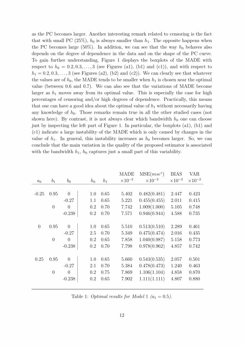
as the PC becomes larger. Another interesting remark related to censoring is the fact
that with small PC (25%), h0 is always smaller than h1. The opposite happens when
the PC becomes large (50%). In addition, we can see that the way h0 behaves also
depends on the degree of dependence in the data and on the shape of the PC curve.
To gain further understanding, Figure 1 displays the boxplots of the MADE with
respect to h0 = 0.2, 0.3, . . . , 3 (see Figures (a1), (b1) and (c1)), and with respect to
h1 = 0.2, 0.3, . . . , 3 (see Figures (a2), (b2) and (c2)). We can clearly see that whatever
the values are of h0, the MADE tends to be smaller when h1 is chosen near the optimal
value (between 0.6 and 0.7). We can also see that the variations of MADE become
larger as h1 moves away from its optimal value. This is especially the case for high
percentages of censoring and/or high degrees of dependence. Practically, this means
that one can have a good idea about the optimal value of h1 without necessarily having
any knowledge of h0. Those remarks remain true in all the other studied cases (not
shown here). By contrast, it is not always clear which bandwidth h0 one can choose
just by inspecting the left part of Figure 1. In particular, the boxplots (a1), (b1) and
(c1) indicate a large instability of the MADE which is only caused by changes in the
value of h1. In general, this instability increases as h0 becomes larger. So, we can
conclude that the main variation in the quality of the proposed estimator is associated
with the bandwidth h1, h0 captures just a small part of this variability.
MADE MSE(mse∗) BIAS VAR
a0 b1 b0 h0 h1 ×10−2 ×10−2 ×10−2 ×10⁻²
-0.25 0.95 0 1.0 0.65 5.402 0.482(0.481) 2.447 0.423
-0.27 1.1 0.65 5.221 0.455(0.455) 2.011 0.415
0 0 0.2 0.70 7.742 1.009(1.000) 5.105 0.748
-0.238 0.2 0.70 7.571 0.946(0.944) 4.588 0.735
0 0.95 0 1.0 0.65 5.510 0.513(0.510) 2.289 0.461
-0.27 2.5 0.70 5.349 0.475(0.474) 2.016 0.435
0 0 0.2 0.65 7.858 1.040(0.987) 5.158 0.773
-0.238 0.2 0.70 7.798 0.978(0.962) 4.857 0.742
0.25 0.95 0 1.0 0.65 5.660 0.543(0.535) 2.057 0.501
-0.27 2.1 0.70 5.384 0.478(0.473) 1.240 0.463
0 0 0.2 0.75 7.869 1.106(1.104) 4.858 0.870
-0.238 0.2 0.65 7.902 1.111(1.111) 4.807 0.880
Table 1: Optimal results for Model 1 (a1 = 0.5).
12

MADE MSE(mse∗) BIAS VAR
a0 b1 b0 h0 h1 ×10−2 ×10−2 ×10−2 ×10⁻²
-0.25 0.95 0 1.3 0.65 5.660 0.497(0.496) 2.900 0.413
-0.27 1.4 0.65 5.503 0.468(0.468) 2.490 0.406
0 0 0.2 0.60 7.992 1.023(1.023) 5.567 0.713
-0.238 0.2 0.65 7.871 1.000(1.002) 5.013 0.748
0 0.95 0 1.4 0.65 5.788 0.522(0.520) 2.718 0.449
-0.27 2.9 0.65 5.589 0.489(0.485) 1.841 0.455
0 0 0.2 0.60 8.108 1.052(1.052) 5.389 0.762
-0.238 0.2 0.60 8.018 0.986(0.986) 5.122 0.723
0.25 0.95 0 1.5 0.65 5.932 0.547(0.547) 2.510 0.484
-0.27 2.8 0.75 5.506 0.470(0.470) 2.394 0.413
0 0 0.2 0.60 8.296 1.101(1.101) 5.289 0.821
-0.238 0.2 0.60 8.282 1.113(1.113) 5.273 0.835
Table 2: Optimal results for Model 2 (a1 = 0.5).
MADE MSE(mse∗) BIAS VAR
a0 b1 b0 h0 h1 ×10−2 ×10−2 ×10−2 ×10⁻²
-0.25 0.95 0 0.7 0.65 6.600 0.700(0.699) 3.417 0.583
-0.27 0.8 0.65 6.506 0.684(0.683) 3.016 0.593
0 0 0.2 0.70 9.003 1.310(1.310) 7.040 0.814
-0.238 0.2 0.70 9.000 1.420(1.402) 7.310 0.885
0 0.95 0 0.9 0.65 6.770 0.742(0.742) 2.966 0.654
-0.27 0.9 0.60 6.667 0.714(0.714) 1.992 0.674
0 0 0.2 0.70 9.201 1.430(1.400) 6.890 0.955
-0.238 0.2 0.70 9.163 1.369(1.369) 6.788 0.908
0.25 0.95 0 0.8 0.60 6.925 0.773(0.773) 2.279 0.721
-0.27 0.9 0.60 6.826 0.752(0.752) 1.890 0.717
0 0 0.2 0.70 9.327 1.441(1.441) 6.688 0.993
-0.238 0.2 0.70 9.012 1.457(1.457) 6.813 0.992
Table 3: Optimal results for Model 3 (a1 = 0.5).
13

0.2 0.5 0.8 1.1 1.4 1.7 2 2.3 2.6 2.9
0.05
0.10
0.15
0.20
0.25
0.30
(a1): Model 2, b1 = 0.95
h0
MA
DE
0.2 0.5 0.8 1.1 1.4 1.7 2 2.3 2.6 2.9
0.05
0.10
0.15
0.20
0.25
0.30
(a2): Model 2, b1 = 0.95
h1
MA
DE
0.2 0.5 0.8 1.1 1.4 1.7 2 2.3 2.6 2.9
0.1
0.2
0.3
0.4
0.5
(b1): Model 2, b1 = 0
h0
MA
DE
0.2 0.5 0.8 1.1 1.4 1.7 2 2.3 2.6 2.9
0.1
0.2
0.3
0.4
0.5
(b2): Model 2, b1 = 0
h1
MA
DE
0.2 0.5 0.8 1.1 1.4 1.7 2 2.3 2.6 2.9
0.1
0.2
0.3
0.4
0.5
(c1): Model 3, b1 = 0
h0
MA
DE
0.2 0.5 0.8 1.1 1.4 1.7 2 2.3 2.6 2.9
0.1
0.2
0.3
0.4
0.5
(c2): Model 3, b1 = 0
h1
MA
DE
Figure 1: Boxplots of mean absolute deviation error (MADE) for Model 2 and Model
3 with a0 = 0.25, a1 = 0.5 and b0 = 0
14
6 Bandwidth selection
The practical performance of any nonparametric regression technique depends strongly
on the smoothing parameters. Choosing an optimal bandwidth is often problematic.
In this section we discuss this problem from a practical point of view in the framework
of censored QR with dependent data. Much research has been carried out in the
area of mean regression with uncensored data. However, when the observations are
subject to censoring, the bandwidth selection question is still unsolved and, even in
the independent case, there is no consistent method available in the literature. There is
also a limited investigation about bandwidth selection in the context of nonparametric
(uncensored) quantile regression. See, for example, Yu and Jones (1998), Zheng and
Yang (1998) and Leung (2005) for more about this subject. One of the data-driven
methods mostly used in the literature is the cross-validation (CV) technique. The CV
criterion approximates the prediction error by removing some observations from the
process. To be precise, let’s focus on the median case and suppose for the moment
that the data are uncensored. In such a situation, one may use the following local
leave-bloc-out CV statistic :
CVx0(h1) = n−1
k
∑
j∈Jk
φ(
medr(Xj) − Yj
)
, (6.1)
where φ is a given positive function, Jk (for some 0 < k ≤ 1) is the set of the nk = ⌊nk⌋nearest neighbor points to x0 and medr is the LL median estimator defined as in (2.2)
but without the observations (Xi, Yi), i = 1, . . . , n, for which |i− j| ≤ r. In this study
we investigate two choices of φ: (1) φ(u) = |u| and (2) φ(u) = u2. These choices
correspond to the L1 and the L2 cross-validation, respectively. The CV rule given by
(6.1) can be seen as a generalization of the conventional global L2-leave-one-out CV
(φ(u) = u2, k = 1 and r = 0). By leaving out more than one observation (r > 0)
we omit the data points that may be highly correlated with (Xj, Yj). On the other
hand, with the local adaptation we try to capture the local behavior of the underlying
process. Of course, in the case of censoring this procedure cannot be used unless the
conditional censoring distribution is known, which is not the case in most practical
situations. As an adaptation of this method to the censored situation, we propose the
following procedure :
Algorithm
(0) Choose a small value for r and k. Let’s say r = 3 and k = 0.25.
(1) For each j in Jk, do the following: (a) denote by Ij the index set of all the data
(Xt, Zt, δt) for which |t− j| > r. (b) For each i ∈ Ij, compute GXi(Zi) as given in
(2.4) but with only the observations (Zt, δt, Xt), t = 1, . . . , n, for which t ∈ Ij. (c)
Calculate medr(Xj) as given by (2.5) but with only the observations (Zt, δt, Xt),
t = 1, . . . , n, for which t ∈ Ij.
15

(2) Calculate the censored cross-validation criterion
CCVx0(h0, h1) = n−1
k
∑
j∈Jk
φ(
medr(Xj) − Zj
)
.
CCVx0has to be evaluated several times with different values for h0 and h1. A natural
selection procedure is to choose (h0, h1) that simultaneously minimize CCVx0(h0, h1).
Here after we will call this approach ‘Method I”. The second method that we propose
is based on the following idea. From the results of the simulation study given in the
previous section, it is clear that a consistent choice of the bandwidth h1 must lead to an
estimator with a relative small error term even if the value of h0 used to estimate Gx is
not the optimal one. Also, whenever h1 is ‘good”, the error terms, as a function of h0
should be relatively stable. As a consequence, we propose the following modification :
Method II
(0) Compute CCVx0(h0, h1) for all possible combinations of h0 and h1 from some
preselected set H0 and H1, respectively.
(1) Pick h1 for which the values in CCVx0(h0, h1), h0 ∈ H0, tend (globally) to be
small and do not change very much (small variation).
(2) Choose h0 that minimizes CCVx0(h0, h1).
It is better to perform the step (1) of this algorithm via a visual inspection. However,
in order to get an automatic approach we propose here to do the following :
• For each value of h1 ∈ H1, let MC(h1) and SC(h1) be the mean and the standard
deviation of CV Vx0(h0, h1), h0 ∈ H0.
• Select the bandwidth h1 that corresponds to the minimum of MC(h1)+λSC(h1).
The parameter λ ≥ 0 determines the trade-off between the mean and the variance.
Choosing a big value for λ means that we penalize those values of h1 that are more
affected by changes in h0.
Due to the high computational cost needed by the cross-validation method, we run
a small simulation study based on 100 replication. Our objective here is to compare
Method I and Method II. For each simulated dataset, we vary the value of (h0, h1) in
0.20, 0.45, . . . , 2.95×0.2, 0.7, . . . , 2.7. From those pairs we select the best one, then
we use the latter to compute the LL median estimator that we denote by med(x0). Let
med(x0) be the LL median estimator based on the optimal (fixed) value of (h0, h1) as
obtained in the last section. As measure of the performance we calculate the empirical
mean of |med(x0) − med(x0)| evaluated over all the simulated data. Almost in all our
simulations we have obtained better results using the L2− cross-validation, that is why
we will not show the results corresponding to the L1 norm. We will also report only
the result for λ = 0, λ = 1 and λ = 3.5, this latter was, in general, the best one
16
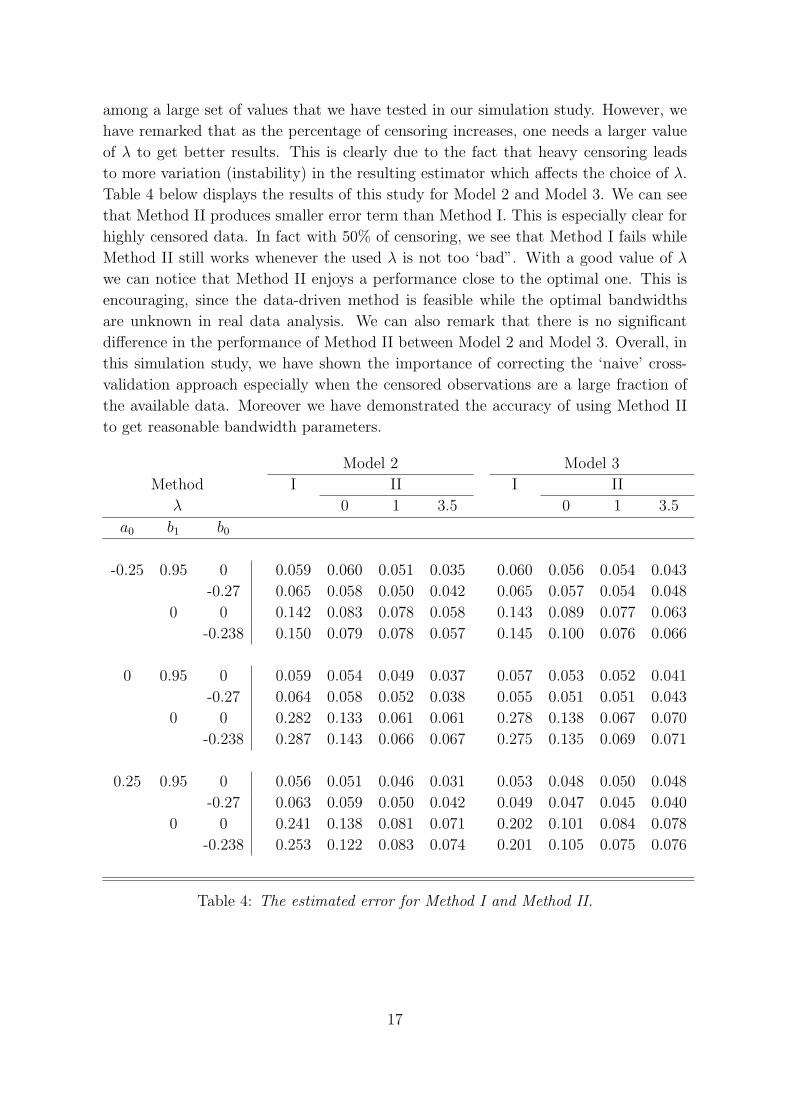
among a large set of values that we have tested in our simulation study. However, we
have remarked that as the percentage of censoring increases, one needs a larger value
of λ to get better results. This is clearly due to the fact that heavy censoring leads
to more variation (instability) in the resulting estimator which affects the choice of λ.
Table 4 below displays the results of this study for Model 2 and Model 3. We can see
that Method II produces smaller error term than Method I. This is especially clear for
highly censored data. In fact with 50% of censoring, we see that Method I fails while
Method II still works whenever the used λ is not too ‘bad”. With a good value of λ
we can notice that Method II enjoys a performance close to the optimal one. This is
encouraging, since the data-driven method is feasible while the optimal bandwidths
are unknown in real data analysis. We can also remark that there is no significant
difference in the performance of Method II between Model 2 and Model 3. Overall, in
this simulation study, we have shown the importance of correcting the ‘naive’ cross-
validation approach especially when the censored observations are a large fraction of
the available data. Moreover we have demonstrated the accuracy of using Method II
to get reasonable bandwidth parameters.
Model 2 Model 3
Method I II I II
λ 0 1 3.5 0 1 3.5
a0 b1 b0
-0.25 0.95 0 0.059 0.060 0.051 0.035 0.060 0.056 0.054 0.043
-0.27 0.065 0.058 0.050 0.042 0.065 0.057 0.054 0.048
0 0 0.142 0.083 0.078 0.058 0.143 0.089 0.077 0.063
-0.238 0.150 0.079 0.078 0.057 0.145 0.100 0.076 0.066
0 0.95 0 0.059 0.054 0.049 0.037 0.057 0.053 0.052 0.041
-0.27 0.064 0.058 0.052 0.038 0.055 0.051 0.051 0.043
0 0 0.282 0.133 0.061 0.061 0.278 0.138 0.067 0.070
-0.238 0.287 0.143 0.066 0.067 0.275 0.135 0.069 0.071
0.25 0.95 0 0.056 0.051 0.046 0.031 0.053 0.048 0.050 0.048
-0.27 0.063 0.059 0.050 0.042 0.049 0.047 0.045 0.040
0 0 0.241 0.138 0.081 0.071 0.202 0.101 0.084 0.078
-0.238 0.253 0.122 0.083 0.074 0.201 0.105 0.075 0.076
Table 4: The estimated error for Method I and Method II.
17

7 Appendix
We start this section by listing all the extra assumptions needed to prove the asymptotic
results given in Section 3. Define H0x(t) = P (Z ≤ t, δ = 0|X = x) =
∫ t
0Fx(s)dGx(s),
the sub-CDF of censored observations.
Assumptions :
(A1) π is such that Qπ(x0) < Tx0.
(A2) (a) f0(x) and Qπ(x) are continuous at x = x0.
(b) Gx(t) and fx(t) are continuous at (x, t) = (x0, β0).
(A3) There exists a neighborhood J of x0 such that :
(a) f′
0 exists and is Lipschitz on J .
(b) x → Hx(t) and x → H0x(t) exist and are Lipschitz on J uniformly in t ≥ 0.
(c) supj≥j∗supu,v∈J fj(u, v) ≤ M∗, for some j∗ ≥ 1 and 0 < M∗ < ∞, where
fj(u, v), j = 1, 2, . . ., denotes the density of (X1, Xj+1).
(A4) K0 is a symmetric density that has a bounded support, say [−1, 1], with a first
derivative K ′0 satisfying |K ′
0(x)| ≤ Λ|x|κ for some κ ≥ 0 and Λ > 0.
(A5) ζπ(x, t) is continuous at (x, t) = (x0, β0).
Proof of Theorem 1. Let
β =
(
β0
β1
)
, Hn =
(
1 0
0 h1
)
and Zt = Zt − β0 − β1(Xt − x0). Put θ = a−1n Hn(β − β), or equivalently θ =
arg minθ Ln(θ), with
Ln(θ) =n∑
t=1
[Zt − anθT Xht][π − δt
¯GXt
(Zt)I(Zt < anθ
T Xht)]K1(Xht).
The ‘quasi-”gradient of −Ln(θ) is given by
Vn(θ) = an
n∑
t=1
[π − δt
¯GXt
(Zt)I(Zt < anθ
T Xht)]XhtK1(Xht).
We also define Vn(θ) to be the same as Vn(θ) but with Gx instead of Gx. To prove
the asymptotic (Bahadur) representation given in Theorem 1, we need the following
lemma whose proof is similar to the proof of Lemma A.4 given in Koenker and Zhao
(1996).
Lemma 1 Let Wn(θ) be a function such that, for any 0 < M < ∞,
(1) −θT Wn(λθ) ≥ −θT Wn(θ), ∀λ ≥ 1
18

(2) sup||θ||≤M ||Wn(θ) + Dθ − An|| = Op(vn),
where ||An|| = Op(1), D is a positive definite matrix, and 0 < vn = O(1). If θn is such
that ||Wn(θn)|| = op(vn), then ||θn|| = Op(1) and θn = D−1An + Op(vn) + op(1).
We will start by showing the following :
(L1) ||[Vn(θ) − Vn(0)] − E[Vn(θ) − Vn(0)]|| = op(1), uniformly in θ over AM := θ :
||θ|| ≤ M.
(L2) ||E[Vn(θ)−Vn(0)]+Dθ|| = o(1), uniformly in θ over AM , where D = f(x0, β0)Λu.
(L3) ||Vn(0)|| = Op(1).
(L4) −θT Vn(λθ) ≥ −θT Vn(θ), ∀λ ≥ 1.
(L5) ||Vn(θ)|| = Op(an).
(L6) sup||θ||≤M ||Vn(θ) − Vn(θ)|| = Op(a−1n h2
0).
From now on, C will denote a generic positive constant independent of n and θ and
whose value may change from line to line. Put a1x = β0 + β1(x − x0), a2
x(θ) = an(θ0 +
θ1(x − x0)/h1).
Proof of (L1)
For any θ and θ such that, ||θ|| ≤ M and ||θ − θ|| ≤ ι, for some M and ι > 0, define
∆in(θ, θ) = an
∑
t
δt
GXt(Zt)
Z∗t (θ, θ)X i
htK1(Xht), i = 0, 1,
with Z∗t (θ, θ) := I(Zt < a1
Xt+ a2
Xt(θ)) − I(Zt < a1
Xt+ a2
Xt(θ)). When no confusion is
possible, we will omit θ and θ in all our notations. Clearly Vn(θ)− Vn(θ) = (∆0n, ∆
1n)T ,
and, by stationarity,
Var[∆0n] = a2
nnVar[δt
GXt(Zt)
Z∗t K1(Xht)] + 2n
n∑
j=1
(1 − j/n)Cj(θ, θ)
≤ a2nnVar[
δt
GXt(Zt)
Z∗t K1(Xht)] + 2n
n∑
j=1
|Cj| (7.1)
where Cj = Cov(
Z∗1 [δ1/GX1
(Z1)]K1(Xh1), Z∗j+1[δj+1/GXj+1
(Zj+1)]K1(Xh(j+1)))
.
Using the fact that |I(y < b)− I(y < a)| ≤ I(b− |a− b| ≤ y ≤ b + |a− b|), we can see
that
|Z∗t (θ, θ)| ≤ I(a1
Xt+ a2
Xt(θ) − Cιan ≤ Zt ≤ a1
Xt+ a2
Xt(θ) + Cιan) := Z∗
t (θ), (7.2)
for some C > 0 and for any t such that |Xt − x0| ≤ h1.
19
By assumptions (A1) and (A2.b), since a1x + a2
x(θ) −−−→x→x0
β0, we can see that, for
n sufficiently large and for any t ∈ t : |Xt − x0| ≤ h1, Zt ≤ a1Xt
+ a2Xt
+ Cιan,GXt
(Zt) ≤ Gx0(β0) + ǫ < 1, for some ǫ > 0. So, as n → ∞,
Var[δt
GXt(Zt)
Z∗t K1(Xht)]
≤ CE[δt
GXt(Zt)
Z∗t K
21(Xht)]
= CE[FXt(a1
Xt+ a2
Xt+ Cιan) − FXt
(a1Xt
+ a2Xt
− Cιan)]K21(Xht)
≤ Cιanh1, (7.3)
where in the last inequality we have used the fact that E(K21(Xht)) = O(h1), and the
fact that, by Taylor development, Fx(a1x+a2
x(θ)+Cιan)−Fx(a1x+a2
x(θ)−Cιan) ≤ Cιan.
Using Cauchy-Schwartz inequality, (7.3) implies that
|Cj| ≤ Var[Z∗j [δj/GXj
(Zj)]K1(Xhj)] = o(h1). (7.4a)
Remark also that, by Assumption (A3.c), we have, for any j ≥ j∗
|Cj| ≤ E|Z∗1Z
∗j+1[δ1/GX1
(Z1)][δj+1/GXj+1(Zj+1)]K1(Xh1)K1(Xh(j+1))|
+ [E|Z∗j [δj/GXj
(Zj)]K1(Xhj)|]2
≤ CE[K1(Xh1)K1(Xh(j+1))] + C[E|K1(Xh1)|]2
≤ Cu20M∗h
21 + C[E(K1(Xht))]
2
= O(h21). (7.4b)
By applying Billingsley’s inequality, see e.g. Corollary 1.1 in Bosq (1998), as n → ∞,
|Cj| ≤ Cj−ν . (7.4c)
Let 0 < kn → ∞. From (7.4) it follows that,∑n
j=1 |Cj| ≤∑j∗
j=1 |Cj| +∑kn
j=j∗+1 |Cj| +∑
j≥kn+1 |Cj| = o(h1) + O(knh21) + O(k1−ν
n ). This together with (7.1) and (7.3) leads
to Var[∆0n] = o(1) + O(knh1) + O(h−1
1 k1−νn ), which converges to 0 whenever kn = h−s
1 ,
with (ν − 1)−1 < s < 1. We deduce that ∆0n −E[∆0
n] = op(1). The same procedure can
also be applied to show that ∆1n − E[∆1
n] = op(1), hence, we conclude that
||[Vn(θ) − Vn(θ)] − E[Vn(θ) − Vn(θ)]|| = op(1). (7.5a)
On the other hand, using (7.2), as n → ∞,
||E[Vn(θ) − Vn(θ)]|| ≤ CanE[n∑
t=1
δt
GXt(Zt)
Z∗t (θ)K1(Xht)] (7.5b)
||Vn(θ) − Vn(θ)|| ≤ Can
n∑
t=1
δt
GXt(Zt)
Z∗t (θ)K1(Xht). (7.5c)
20

Note that the right part of those inequalities does not depend on θ. Moreover, following
the same treatment as we have done above, see (7.3),
E[an
∑
t
δt
GXt(Zt)
Z∗t K1(Xht)] ≤ Cι
Therefore, by letting ι → 0, we get
||E[Vn(θ) − Vn(θ)]|| = op(1) ||Vn(θ) − Vn(θ)|| = op(1). (7.5d)
The desired uniform consistency given in (L1) follows from (7.5) by using a chaining
argument as in Hallin et al. (2005).
Proof of (L2)
First note that, by definition of Vn(θ),
E[Vn(θ) − Vn(0)] = nanE[b(θ,Xt)XhtK1(Xht)],
where b(θ, x) = Fx(a1x) − Fx(a
1x + a2
x(θ)).
By Taylor development, we have that, for some 0 < η < 1, b(θ, x) = −a2x(θ)fx(a
1x +
ηa2x(θ)). This implies that,
E[Vn(θ) − Vn(0)] = −h−11 E[XhtX
ThtfXt
(a1Xt
+ ηa2Xt
(θ))K1(Xht)]θ.
To complete the proof observe that, by Assumption (A2.a) and (A2.b),
sup||θ||≤M,|x−x0|≤h1
|fx(a1x + ηa2
x(θ)) − fx0(β0)| → 0, and
1
h1
∫(
x − x0
h1
)i
K1
(
x − x0
h1
)
f0(x)dx → f0(x0)ui, i = 0, 1, 2.
Proof of (L3)
Remark that Vn(0) = (V 0n (0), V 1
n (0))T , with
V in(0) = an
∑
t
[π − I(Zt < a1Xt
)δt/GXt(Zt)]X
ihtK1(Xht), i = 0, 1.
We have that
E[V 0n (0)] = nan
∫
(π − Fx(a1x))K1(
x − x0
h1
)f0(x)dx.
By first and second order Taylor development of t → Fx(t) and x → Qπ(x), respectively,
we can see that, for some 0 < η1, η2 < 1,
π − Fx(a1x) = Fx(Qπ(x)) − Fx(a
1x)
= [Qπ(x) − a1x]fx(a
1x + η1(Qπ(x) − a1
x))
= 2−1(x − x0)2Qπ(x + η2(x − x0))fx(a
1x + η1(Qπ(x) − a1
x)).
21

By assumption (A2.a) and (A2.b) and the fact that nh51 = O(1) (see assumption (i) in
the statement of the theorem), we deduce that E[V 0n (0)] = nanh
31(u2/2)Qπ(x0)f(x0, β0)+
o(1) = O(nanh31) + o(1) = O(1). Now, we need to show that V(V 0
n (0)) = O(1).
This can be done by first noticing that Var[π − I(Zt < a1Xt
)δt/GXt(Zt)]K1(Xht) ≤
CE[K21(Xht)] = O(h1) and then by following a similar treatment as we have done above
for Var(∆0n) in the proof of (L1). So, this shows that V 0
n (0) = Op(1). Similarly one
can also verify that V 1n (0) = Op(1). From this we conclude that Vn(0) = Op(1).
Proof of (L4)
Using the fact that δt/¯GXt
(Zt) and K1(Xht) are nonnegative quantities, it is easy to
check that , for a given θ, λ → −θVn(λθ) is a nondecreasing function which implies the
desired result.
Proof of (L5)
(L5) is a direct application of the following result :
Lemma 2 For any random vectors Xt ∈ Rp and (At, Bt, Ct)
T ∈ R3, t = 1 . . . , n, let
θn = arg minθ∈Rp
∑
t[At − θTXt][π − BtI(At < θTXt)]Ct. If Bt and Ct ≥ 0, Xt is
continuous and ||θn|| < ∞ then, with probability one
||∑
t
Xt[π − BtI(At < θTn Xt)]Ct|| ≤ p max
t||BtCtXt||
The proof of this lemma follows along the same lines as in the proof of Lemma A.2
in Ruppert and Carroll (1980).
Proof of (L6)
Since K1 is nonnegative,
an||Vn(θ) − Vn(θ)|| ≤ [1
nh1
n∑
i=1
K1
(
Xi − x0
h1
)
] supt∈An(θ)
|GXt(Zt) − GXt
(Zt)|¯GXt
(Zt)GXt(Zt)
,
where An(θ) = t : |Xt − x0| ≤ h1 and Zt < β0 + β1(Xt − x0) + anθT Xht.For n sufficiently large and for any θ such that ||θ|| ≤ M , using the fact that K1
has a compact support, assumption (A1) and (A2.b), one can find a neighborhood
J ⊂ J of x0 and an ǫ > 0 such that, if t ∈ An(θ) then Xt ∈ J , Zt ≤ β0 + ǫ < Tx0and
GXt(Zt) ≤ Gx0
(β0) + ǫ < 1. On the other hand, by Theorem 3.1(II) in El Ghouch and
Van Keilegom (2006), we have that
supx∈J
sups∈[0,β0+ǫ]
|Gx(s) − Gx(s)| = Op(h20),
whenever Assumptions (A3) and (A4) and Assumptions (ii) and (iv) given in the
statement of the theorem, are fulfilled. To conclude the proof, one can easily check
22
that, by Assumptions (A2.a) and (A3.c),
1
nh1
n∑
i=1
K1
(
Xi − x0
h1
)
= Op(1).
Now that we have shown (L1)-(L6), we continue with the proof of Theorem 1. (L1),
(L2) and (L6) imply that
||Vn(θ) + Dθ − Vn(0)|| ≤ ||Vn(θ) − Vn(θ)|| + ||(Vn(θ) − Vn(0)) − E(Vn(θ) − Vn(0))||+ ||E(Vn(θ) − Vn(0)) + Dθ||
= op(1) + Op(a−1n h2
0), (7.6)
uniformly over θ : ||θ|| ≤ M. This together with (L3), (L4), (L5), (iii) (see statement
of the theorem) and Lemma 1, implies that ||θ|| = Op(1), which, by (7.6), leads to
θ = D−1Vn(0) + Op(a−1n h2
0) + op(1)
= Λ−1u /f(x0, β0)[an
∑
t
etXhtK1(Xht) + Bn] + Op(a−1n h2
0) + op(1),
where et is defined in the theorem and Bn = (B0n, B
1n)T , with
Bin = an
n∑
i=1
[I(Zt < Qπ(Xt)) − I(Zt < a1Xt
)]δt
GXt(Zt)
X ihtK1(Xht), for i = 0, 1.
To get exactly the asymptotic expression given in Theorem 1, and so to conclude the
proof, we still have to show that Bn = (a−1n h2
1/2)(u2, u3)T Qπ(x0)f(x0, β0)+op(a
−1n h2
1)+
op(1). This can be done by checking that, for i = 0, 1,
E(Bin) = nanE[FXt
(Qπ(Xt)) − FXt(a1
Xt)]X i
htK1(Xht)= a−1
n h21/2[Qπ(x0)f(x0, β0)ui+2 + o(1)], (7.7a)
andVar(Bi
n) = o(1). (7.7b)
(7.7a) and (7.7b) can be proved by following the same treatment as we have done above
for E[V in(0)], see the proof of (L3), and for Var[∆i
n], see the proof of (L1), respectively.
Proof of Theorem 2. In order to establish the asymptotic normality, it suffices, by
Theorem 1, to show that
An := an
n∑
t=1
etXhtK1(Xht)L−→ N (0, f0(x0)ζ(x0, β0)Ωv) .
23

By the Cramer-Wold device, this is equivalent to showing that for any linear combina-
tion cT AnL−→ N
(
0, f0(x0)ζ(x0, β0)cT Ωvc
)
. First note that E(et|Xt) = π−FXt(Qπ(Xt)) =
0, and
E(e2t |Xt) = E[
δt
G2Xt
(Zt)I(Zt < Qπ(Xt))|Xt] − π2 = ζπ(Xt, Qπ(Xt)).
On the other hand, by assumption (A2.a) and (A5), we have that
1
h1
∫
ζπ(x,Qπ(x))
(
x − x0
h1
)i
K1
(
x − x0
h1
)
f0(x)dx → ζπ(x0, β0)f0(x0)vi, i = 0, 1, 2.
This implies that Var[etcT XhtK1(Xht)] = h1[f0(x0)ζπ(x0, β0)c
T Ωvc + o(1)]. Now, by
stationarity, Var[cT An] = 1/(nh1)
nVar[etcT XhtK1(Xht)] + 2n
∑n
j=1(1 − j/n)C+j
,
where C+j = Cov(e1c
T Xh1K1(Xh1), ej+1cT Xh(j+1)K1(Xh(j+1))). Using Assumption (A3.c)
(with j∗ = 1), we can easily see that C+j ≤ CE[K1(Xh1)K1(Xh(j+1))] = O(h2
1), for any
j ≥ 1. So, by an appropriate choice of kn → 0 and using Billingsley’s inequality,∑n
j=1 |C+j | ≤
∑kn
j=1 |Cj| +∑
j≥kn+1 |C+j | = O(knh2
1) + O(k1−νn ) = o(h1). Thus, we have
shown that E[cT An] = 0, and Var[cT An] → f0(x0)ζ(x0, β0)cT Ωvc.
It remains to prove that cT An is asymptotically normal. This can be done by
using the well known small-blocks and large-blocks technique and then by verifying
the standard Lindeberg-Feller conditions exactly as it was done, for example, in Masry
and Fan (1997). Details are omitted.
Corresponding address :
Universite catholique de Louvain
Institute of Statistics
20, Voie du Roman Pays
B-1348 Louvain-la-Neuve
Belgium
Email: [email protected]
References
Alavi, A. and A. Thavaneswaran (2002). Nonparametric estimators for censored cor-
related data. Comm. Statist. Theory Methods 31, 977–985.
Bang, H. and A. A. Tsiatis (2002). Median regression with censored cost data. Bio-
metrics 58, 643–649.
Beran, R. (1981). Nonparametric regression with randomly censored survival data.
Technical report, Dept. Statist., Univ. California, Berkeley.
24

Bosq, D. (1998). Nonparametric Statistics for Stochastic Processes. New York:
Springer.
Bradley, R. (1986). Basic properties of strong mixing conditions. In Dependence in
Probability and Statistics: A Survey of Recent Results, pp. 165–192. Birkhauser,
Boston (eds. E. Eberlein and M. S. Taqqu).
Cai, Z. (2002). Regression quantiles for time series data. Econometric Theory 18,
169–192.
Chernozhukov, V. and H. Hong (2002). Three-step censored quantile regression and
extramarital affairs. J. Amer. Statist. Assoc. 97, 872–882.
Dabrowska, D. M. (1992). Nonparametric quantile regression with censored data.
Sankhya Ser. A 54, 252–259.
Doukhan, P. (1994). Mixing: Properties and Examples. Lecture Notes in Statistics.
Springer.
Eastoe, E. F., C. J. Halsall, J. E. Heffernan, and H. Hung (2006). A statistical compari-
son of survival and replacement analyses for the use of censored data in a contaminant
air database: A case study from the canadian arctic. Atmospheric Environment 40,
6528–6540.
El Ghouch, A. and I. Van Keilegom (2006). Nonparametric regression with dependent
censored data. Discussion paper DP0620, Institute of Statistics, Universite catholique
de Louvain. http://www.stat.ucl.ac.be/ISpub/ISdp.html (under revision for Scand.
J. Statist.).
Fan, J. and I. Gijbels (1996). Local Polynomial Modelling and its Applications, Vol-
ume 66 of Monographs on Statistics and Applied Probability. London: Chapman &
Hall.
Fan, J., T. C. Hu, and Y. K. Truong (1994). Robust non-parametric function estima-
tion. Scand. J. Statist. 21, 433–446.
Fitzenberger, B. (1997). A guide to censored quantile regressions. In Robust inference,
Volume 15 of Handbook of Statistics, pp. 405–437. Amsterdam: North-Holland.
Gannoun, A., J. Saracco, and K. Yu (2003). Nonparametric prediction by conditional
median and quantiles. J. Statist. Plann. Inference 117, 207–223.
Gannoun, A., J. Saracco, A. Yuan, and G. E. Bonney (2005). Non-parametric quantile
regression with censored data. Scand. J. Statist. 32, 527–550.
Hallin, M., Z. Lu, and K. Yu (2005). Local linear spatial quantile regression.
Technical report TR0552, Interuniversity Attraction Pole-Network in Statistics.
http://www.stat.ucl.ac.be/IAP/publication tr.html.
25

Honda, T. (2000). Nonparametric estimation of a conditional quantile for α-mixing
processes. Ann. Inst. Statist. Math. 52, 459–470.
Honore, B., S. Khan, and J. L. Powell (2002). Quantile regression under random
censoring. J. Econometrics 109, 67–105.
Hunter, D. R. and K. Lange (2000). Quantile regression via an MM algorithm. J.
Comput. Graph. Statist. 9, 60–77.
Koenker, R. (2005). Quantile Regression, Volume 38 of Econometric Society Mono-
graphs. Cambridge: Cambridge University Press.
Koenker, R. and G. Bassett, Jr. (1978). Regression quantiles. Econometrica 46, 33–50.
Koenker, R. and Y. Bilias (2001). Quantile regression for duration data: A reappraisal
of the Pennsylvania reemployment bonus experiments. Empirical Economics 26,
199–220.
Koenker, R. and O. Geling (2001). Reappraising medfly longevity: a quantile regression
survival analysis. J. Amer. Statist. Assoc. 96, 458–468.
Koenker, R. and Q. Zhao (1996). Conditional quantile estimation and inference for
ARCH models. Econometric Theory 12, 793–813.
Leconte, E., S. Poiraud-Casanova, and C. Thomas-Agnan (2002). Smooth conditional
distribution function and quantiles under random censorship. Lifetime Data Anal. 8,
229–246.
Leung, D. H.-Y. (2005). Cross-validation in nonparametric regression with outliers.
Ann. Statist. 33, 2291–2310.
Lipsitz, S. R. and J. G. Ibrahim (2000). Estimation with correlated censored survival
data with missing covariates. Biostatistics 1, 315–327.
Masry, E. and J. Fan (1997). Local polynomial estimation of regression functions for
mixing processes. Scand. J. Statist. 24, 165–179.
Portnoy, S. (2003). Censored regression quantiles. J. Amer. Statist. Assoc. 98, 1001–
1012.
Powell, J. L. (1986). Censored regression quantiles. J. Econometrics 32, 143–155.
Ruppert, D. and R. J. Carroll (1980). Trimmed least squares estimation in the linear
model. J. Amer. Statist. Assoc. 75, 828–838.
Stute, W. (2005). Consistent estimation under random censorship when covariates are
present. Scand. J. Statist. 32, 527–550.
26

Van Keilegom, I. and N. Veraverbeke (1998). Bootstrapping quantiles in a fixed design
regression model with censored data. J. Statist. Plann. Inference 69, 115–131.
Yin, G. and J. Cai (2005). Quantile regression models with multivariate failure time
data. Biometrics 61, 151–161.
Yu, K. and M. C. Jones (1998). Local linear quantile regression. J. Amer. Statist.
Assoc. 93, 228–237.
Yu, K., Z. Lu, and J. Stander (2003). Quantile regression: applications and current
research areas. The Statistician 52, 331–350.
Zhao, Y. and H. C. Frey (2004). Quantification of variability and uncertainty for
censored data sets and application to air toxic emission factors. Risk Analysis 24,
1019–1034.
Zheng, Z. G. and Y. Yang (1998). Cross-validation and median criterion. Statist.
Sinica 8, 907–921.
27