Zeiss LSM 510 Meta inverted confocal manual *adapted from the Duke University Light Microscopy Core Facility manual

Power Up

1. Turn on the mercury lamp (if required) and sign in the log book, recording lamp hours. 2. Turn on the PC and log in using your network username and password (you will enter this

twice). 3. If using the multiphoton laser, turn the key from “Standby” to “on”. 4. Switch remote to “on”.

Open the Software

1. Double-click the 510 icon on the desktop. The LSM switchboard appears.

Make sure Scan New Images is activated.

Figure 1) 510 AIM Switchboard

"Use Existing Images" is an off-line mode used for image analysis only. In this mode, the hardware can't be controlled by the software. If imaging is attempted in this mode, the laser scan is emulated.

2. Click on Start Expert in the Switchboard.

Finding Your Specimen in the Eyepieces

The objectives and fluorescent filters on the Axiovert 200M stand are motorized and can be controlled in the software via the Acquire>Micro submenu. You may want to find and view your specimen under transmitted light (plain white light) or fluorescence (reflected light), or both.

• To be able to see through the eyepieces using transmitted light, “Vis” must be selected in the Acquire menu, the transmitted light button must be depressed, and the reflector must be set to “none.”

• To see fluorescence, the “Vis” button must be depressed, the reflected light button must be depressed, and the reflector must be set to your desired color.

When you've located something you'd like to confocal, click the LSM button on the software panel.

Acquiring Images

Turn On the Lasers

Select Acquire>Laser submenu will open the "Laser Control" window with a list of available lasers.

Laser Lines (nm) Colour of fluorophores

Examples of fluorophores

Chameleon 720-950 Blue, Green DAPI, Alexa 350, GFP Argon 458 477 488

514 Green (Cyan and

Yellow) GFP, Alexa 488, FITC,

543 HeNe 594 Red Alexa 594, texas red, mCherry

633 HeNe 633 Far-red Alexa 633, CY5

Turn on only the laser(s) you need to excite the fluorophores in your sample.

Argon laser: click standby to warm it up. After the initial warm-up period, the on button will appear allowing the laser to be fully activated. Move the power output slider to about 50%. To turn on any of the other lasers, simply click the appropriate "On" buttons - no warm-up is required for ignition.

We try to minimize the number of times a laser is turned on or off - if somebody will use the laser within 2 hours leave it on (Argon laser in standby). Check the reservation schedule to see the laser usage scheduled before and after your session. Turn off any lasers you don't need that may have been left on for you by the previous user, as long as anyone scheduled after you won't use them within 2 hours of your imaging session.

Choose a configuration

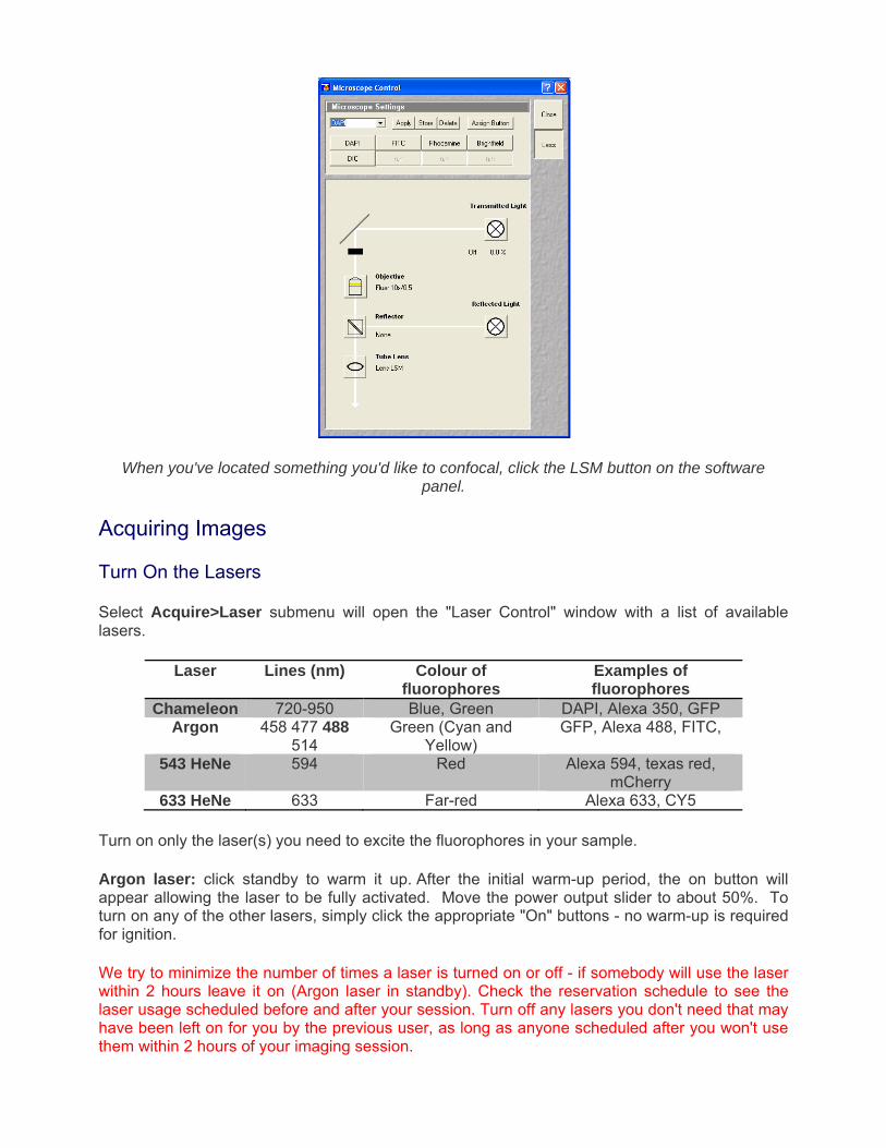
1. A filter configuration for the particular fluorophores you are using can be loaded via the "Configuration Control" window. Open it by selecting the Acquire>Config submenu. Refer to Fig 2.

2. Single Track mode is for single channel imaging or simultaneous excitation of multiple channels; in Multi Track mode the laser scans multiple channels sequentially, which can be useful when bleedthrough is a problem. Select whichever is appropriate for your imaging needs.

3. The saved configuration button on the right side of the "Configuration Control" window opens the "Track Configurations" window. Here, the dropdown menu has a list of typical color configurations for general use. Choose whichever one is appropriate for your specimen.

4. Click Apply to load the laser & filter settings for that configuration.

Figure 2) Selecting Your Imaging Configuration

Scan control

Acquire>Scan opens the "Scan Control" window - the main dialog box for acquiring images.

Adjustments under the mode tab . . .

• Objective Lens & Image Size: choose a field size using the buttons provided (512x512 pixels is the default). But it is also possible to enter different values for X and Y if preferred.

• Speed: Reducing the scan speed can improve a noisy image; faster scan speeds are used to find regions of interest (like during the Fast XY function). ***Remember: the slower the scan speed, the more chance of bleaching your specimen, especially if it’s a sensitive fluorophore.

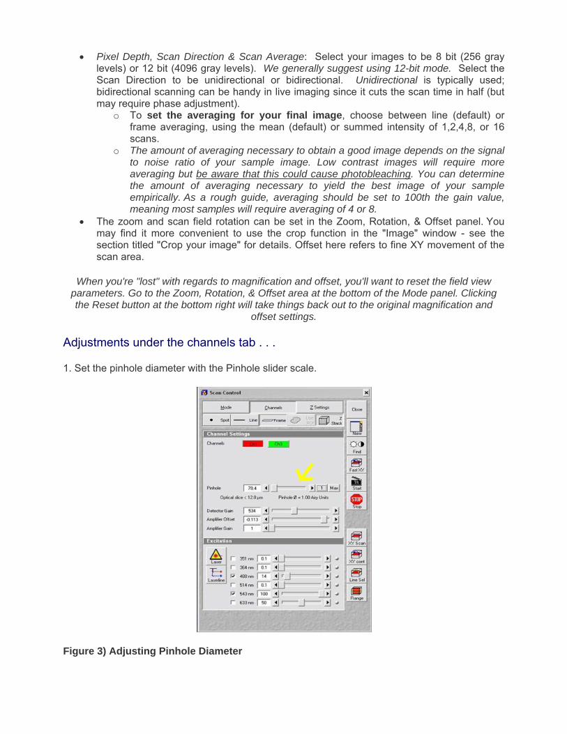
• Pixel Depth, Scan Direction & Scan Average: Select your images to be 8 bit (256 gray levels) or 12 bit (4096 gray levels). We generally suggest using 12-bit mode. Select the Scan Direction to be unidirectional or bidirectional. Unidirectional is typically used; bidirectional scanning can be handy in live imaging since it cuts the scan time in half (but may require phase adjustment).

o To set the averaging for your final image, choose between line (default) or frame averaging, using the mean (default) or summed intensity of 1,2,4,8, or 16 scans.

o The amount of averaging necessary to obtain a good image depends on the signal to noise ratio of your sample image. Low contrast images will require more averaging but be aware that this could cause photobleaching. You can determine the amount of averaging necessary to yield the best image of your sample empirically. As a rough guide, averaging should be set to 100th the gain value, meaning most samples will require averaging of 4 or 8.

• The zoom and scan field rotation can be set in the Zoom, Rotation, & Offset panel. You may find it more convenient to use the crop function in the "Image" window - see the section titled "Crop your image" for details. Offset here refers to fine XY movement of the scan area.

When you're "lost" with regards to magnification and offset, you'll want to reset the field view parameters. Go to the Zoom, Rotation, & Offset area at the bottom of the Mode panel. Clicking the Reset button at the bottom right will take things back out to the original magnification and

offset settings.

Adjustments under the channels tab . . .

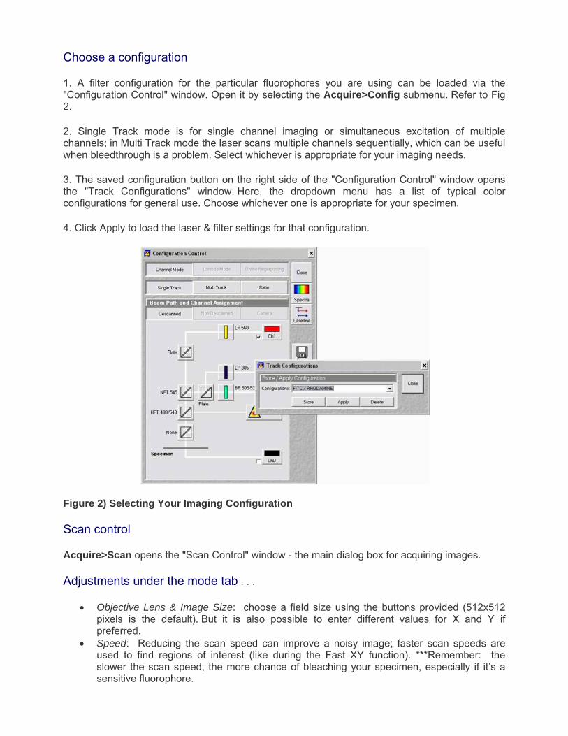
1. Set the pinhole diameter with the Pinhole slider scale.

Figure 3) Adjusting Pinhole Diameter

If you are using the Chameleon laser (ex: DAPI) set it’s pinhole to Max. For the other lasers, the smaller the pinhole, the thinner the optical slice will be and the less light will be collected. A pinhole set to 1 Airy unit (click the 1 button) will have optimal resolution. However, you will

probably need to adjust this according to your sample's fluorescence, using larger Airy values for dim samples.

For multi-fluorophore imaging, it is usually advisable to set the pinholes for each channel to produce equivalently thick optical slices.

2. Adjust % laser transmission(s) in the Excitation Of Track panel at the bottom of the window. Doing so sets the % laser power let through by the AOTF.

3. Press "Find" to acquire a preliminary image using automatic setting of gain and offset. An image display window will open and the output of the find scan will be displayed.

4. Click the Fast XY button to the right in the "Scan Control" window. While the laser is scanning, use the XY Stage Controller to search for an interesting area or frame up a good image. Adjust the fine focus on the microscope body. Clicking "Stop" in the Scan Control window will turn off the Fast XY continuous scanning.

Optimize your image

The preliminary image, whether too dim or too bright, usually needs to be optimized. The PMTs need to be adjusted according to the fluorescence intensity of the sample.

1. Under the Channel Settings panel in "Scan Control", colored buttons represent each channel you're scanning. Select each channel separately by clicking on the corresponding button - contrast & brightness adjustments can be made to individual channels only when activated in this way.

2. Select Palette in the image window's Select toolbar. From the Color Palette List, select Range Indicator. In this palette, pixels with intensity of 0 are blue and pixels with intensity of 255 (for 8 bit images) are displayed red.

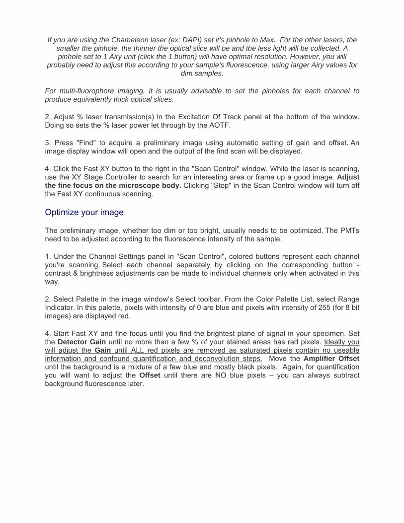
4. Start Fast XY and fine focus until you find the brightest plane of signal in your specimen. Set the Detector Gain until no more than a few % of your stained areas has red pixels. Ideally you will adjust the Gain until ALL red pixels are removed as saturated pixels contain no useable information and confound quantification and deconvolution steps. Move the Amplifier Offset until the background is a mixture of a few blue and mostly black pixels. Again, for quantification you will want to adjust the Offset until there are NO blue pixels – you can always subtract background fluorescence later.

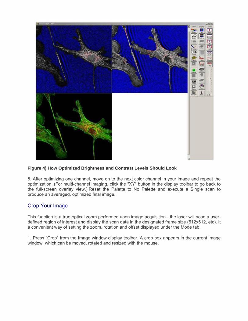
Figure 4) How Optimized Brightness and Contrast Levels Should Look

5. After optimizing one channel, move on to the next color channel in your image and repeat the optimization. (For multi-channel imaging, click the "XY" button in the display toolbar to go back to the full-screen overlay view.) Reset the Palette to No Palette and execute a Single scan to produce an averaged, optimized final image.

Crop Your Image

This function is a true optical zoom performed upon image acquisition - the laser will scan a user-defined region of interest and display the scan data in the designated frame size (512x512, etc). It a convenient way of setting the zoom, rotation and offset displayed under the Mode tab.

1. Press "Crop" from the Image window display toolbar. A crop box appears in the current image window, which can be moved, rotated and resized with the mouse.

Figure 5) The Crop Box Overlaid On a Loaded Image

2. To set the offset, position the mouse inside the crop box. The cursor will change to an icon of perpendicular arrows indicating direction in the X and Y dimensions. Use the left mouse button to drag and drop the crop box to the desired offset position.

3. To set the zoom of the scan, position the mouse over a corner of the crop box. The cursor will change to an icon indicating zoom in/out relative to a centerpoint. Left-click and drag until the desired zoom has been achieved.

4. To rotate the scan, left-click on an end of the crosshairs and drag to set your desired rotation. The cursor will change to a circular icon indicating rotation around a centerpoint. The blue side of the crop box indicates the top of the new cropped scan that will be acquired.

5. To make your image frame rectangular, left-click on any of the intersections between the crosshair and sides of the square. The cursor will change to up/down or side-to-side arrowheads, depending on the dimension you want to change. That side can then be dragged and dropped to the desired frame size.

Pressing "single" will rescan with the modified zoom etc settings

Save your image

Create a New Database

1. Select the File>New submenu. This will open the "Create New Database" window.

2. Select the server location where you want the database stored using the drop down list of folders in the Create in field. You should save your images to your directory your shared directory on the network.

3. Enter a name for the new database in the File name field. 4. Click Create. Databases created on the LSM510 will be in a proprietary *.mdb format.

Files in these databases are in a proprietary .lsm format, but they can be exported to standard formats for use in other programs.

Saving each individual image or stack

1. Select Save in the bottom right hand corner of the display window toolbar. Data is overwritten by the next image unless saved.

2. In the "Save Image and Parameter As" window that appears, select the database to which you want the image stored by selecting its name in the Database (MDB) field. (you can also create a new database here).

Users should generally save their images either to their own user folder on the fileserver or directly to a USB memory drive. Any images saved on the hard-drives are unsafe and are subject

to deletion WITHOUT WARNING.

Advanced Imaging Functions

Z-sectioning

To collect a series of images at different points along the z-axis the settings can be inputted in two ways: Z Sectioning or Mark First/Last.

• Z-sectioning - takes x slices at a particular z interval • Mark first/last - set the top and bottom of your sample and select either the interval or

number of slices (the other is calculated for you)

Both of the methods described here assume that the user has optimized and set all imaging parameters, including pinhole size, detector gain/offset, scan time and averaging described above.

Z Sectioning Method

1. This method assumes the user has prior knowledge of the specimen's thickness and/or is willing to guesstimate thickness. Select Z Stack at the top in the "Scan Control" window - doing this will activate the Z Settings panel.

2. Click on the Z Sectioning tab and select Keep Interval. This will keep the z slice size constant, even if you later decide to change the Num Slices or the upper and lower limits in your stack.

3. Type in the desired interval for your z stack in the Interval (um) field of the Z Sectioning tab. If necessary, look up the optimal z interval thickness by clicking Z Slice at the top of the Z Settings box. This will open the "Optimal Slice" window. Assuming you have already adjusted your pinholes as described in "Acquire Menu: Collect An XY Section", your optimal z interval thickness for the objective currently in use will be displayed in this window. Clicking Optimal Interval in the

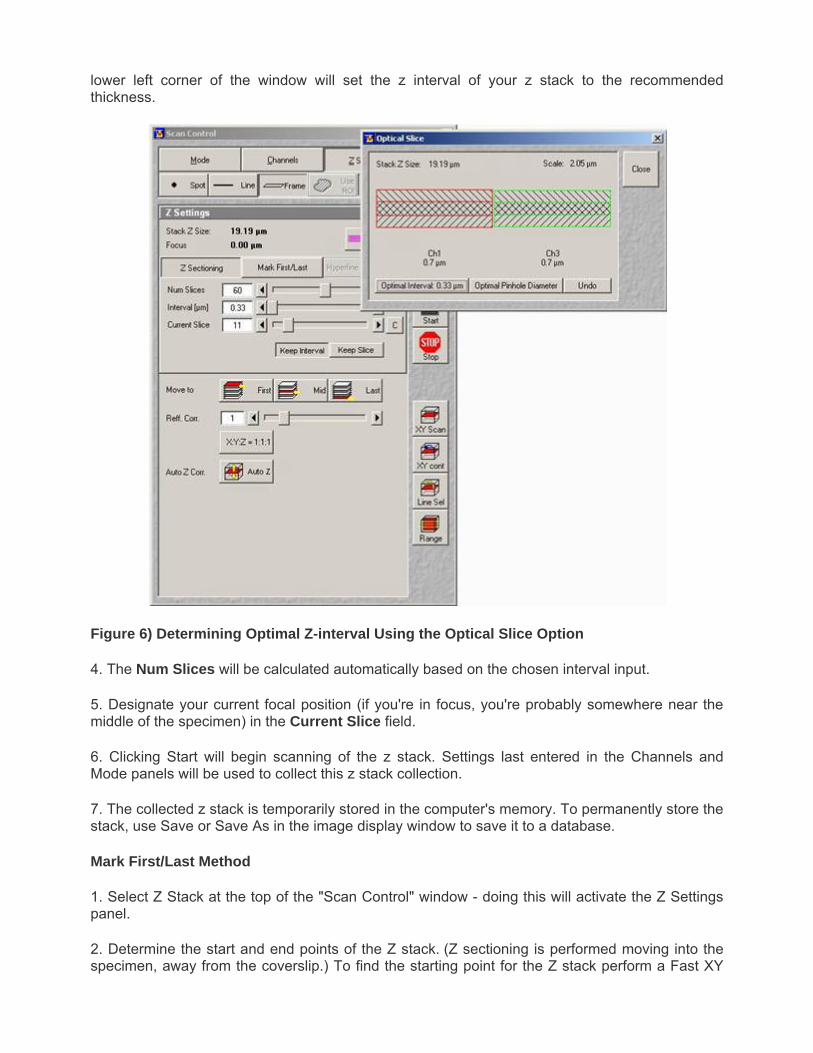
lower left corner of the window will set the z interval of your z stack to the recommended thickness.

Figure 6) Determining Optimal Z-interval Using the Optical Slice Option

4. The Num Slices will be calculated automatically based on the chosen interval input.

5. Designate your current focal position (if you're in focus, you're probably somewhere near the middle of the specimen) in the Current Slice field.

6. Clicking Start will begin scanning of the z stack. Settings last entered in the Channels and Mode panels will be used to collect this z stack collection.

7. The collected z stack is temporarily stored in the computer's memory. To permanently store the stack, use Save or Save As in the image display window to save it to a database.

Mark First/Last Method

1. Select Z Stack at the top of the "Scan Control" window - doing this will activate the Z Settings panel.

2. Determine the start and end points of the Z stack. (Z sectioning is performed moving into the specimen, away from the coverslip.) To find the starting point for the Z stack perform a Fast XY

scan and focus toward the coverslip (rotate fine focus knob toward you) until you reach the point at which you'd like to begin the Z stack. Stop the Fast XY scanning.

3. Click Mark First in the Mark First/Last tab in the Z Settings panel.

4. Start another Fast XY scan and turn the fine focus knob away from you focusing down through your specimen until you reach the point at which you'd like to end the Z stack. Stop the Fast XY scanning.

5. Click Mark Last to set the end point of the stack.

6. Assuming you have already adjusted your pinholes as described in "Acquire Menu: Collect An XY Section", look up the optimal z interval thickness by clicking Z Slice at the top of the Z Settings box. This will open the "Optimal Slice" window.

7. Optimal z interval thickness for the objective currently in use will be displayed in this window. Clicking Optimal Interval in the lower left corner of the window will set the z interval of your z stack to the recommended thickness.

8. Start will begin scanning of the z stack. Settings last entered in the Channels and Mode panels will be applied to this z stack collection.

9. The collected z stack is temporarily stored in the computer's memory. To permanently store the stack, use Save or Save As in the image display window to save it to a database.

Time series

The Time Series is a versatile software function that is useful in a variety of situations - from collecting single confocal images or entire z stacks over time to more sophisticated applications such as FRAP. If desired, a delay between the beginning of one scan process to the beginning of the next can be set. It is important to note that Time Series works at only one location on the slide. To apply the Time Series function to multiple stage locations, you will have to use the Multitime macro.

The following instructions are for applying a basic Time Series. It is assumed that the user has optimized and set all imaging parameters beforehand (pinhole size, detector gain/offset, scan time, averaging, and if desired, z stack). Refer to previous sections for more details on adjusting these settings.

1. Select the Acquire>Time Series submenu.

2. In the Start Series panel, choose between a Manual start or a timed start via Time. Most users want a manual start. If a timed start is desired, enter a start time in the Time (h:m:s) field. The time series will start when the set time is reached according to the computer's clock.

3. In the End Series panel, enter the number of time points desired in the Number field if a Manual end is selected. For a timed end point, depress Time and enter the end time in the Time (h:m:s) field.

In determining an experiment's length and the number of time points needed it is important to consider the scan time and averaging settings (see the Speed section of the Mode panel in "Scan

Control"). Both parameters influence how long it takes the laser to clear the scan field and thereby define the minimum time between time points.

4. The next panel you encounter will be either Time Interval or Time Delay, depending on the settings of your Time Series register (see Options--> Settings). Time Delay is defined as the end of one scan process to the beginning of the next, while Time Interval is the time between the beginning of one scan process to the beginning of the next. Either panel, Time Interval or Time Delay, permits time series scan parameters to be activated or changed from experiment to experiment.

You may load & Apply previously saved time series settings using the pulldown menu in either of these panels. Or you may choose to manually enter scan parameters into the Time and Unit fields. If you foresee performing other experiments with identical time scan settings, you should Store your manually entered settings to the dropdown list for easy reference in the future.

5. Click Start T in the right-hand side of the "Time Series" window to start your time series.

6. The collected time series is temporarily stored in the computer's memory. To permanently store the series, use Save or Save As in the image display window to save it to a database.

Ending your session

Remove your sample from the stage and clean any oil objectives you used. Please let us know of any problems.

Check the reservation schedule to see if/when the next reservation is scheduled:

If someone else is scheduled to use the microscope within 2 hours...

• Put the Argon laser into standby and turn off any lasers that won't be used by the next person, leaving on the ones indicated on the booking calendar

• Exit the software • Select the "Log Off" command from the Start menu of the desktop and leave the system

on. • Sign the logbook

If you are the last scheduled session of the day or for more than 2 hours...

• Turn off all the lasers in the Acquire>laser box (You must wait for the Argon laser to cool if it is on) and exit the software

• Select "Shut down computer" command in the Start menu of the desktop. The computer and monitors will power down automatically.

• Turn off the Remote switch • Turn of the key • Turn of the arc lamp • Sign the logbook and record the lamp hours.

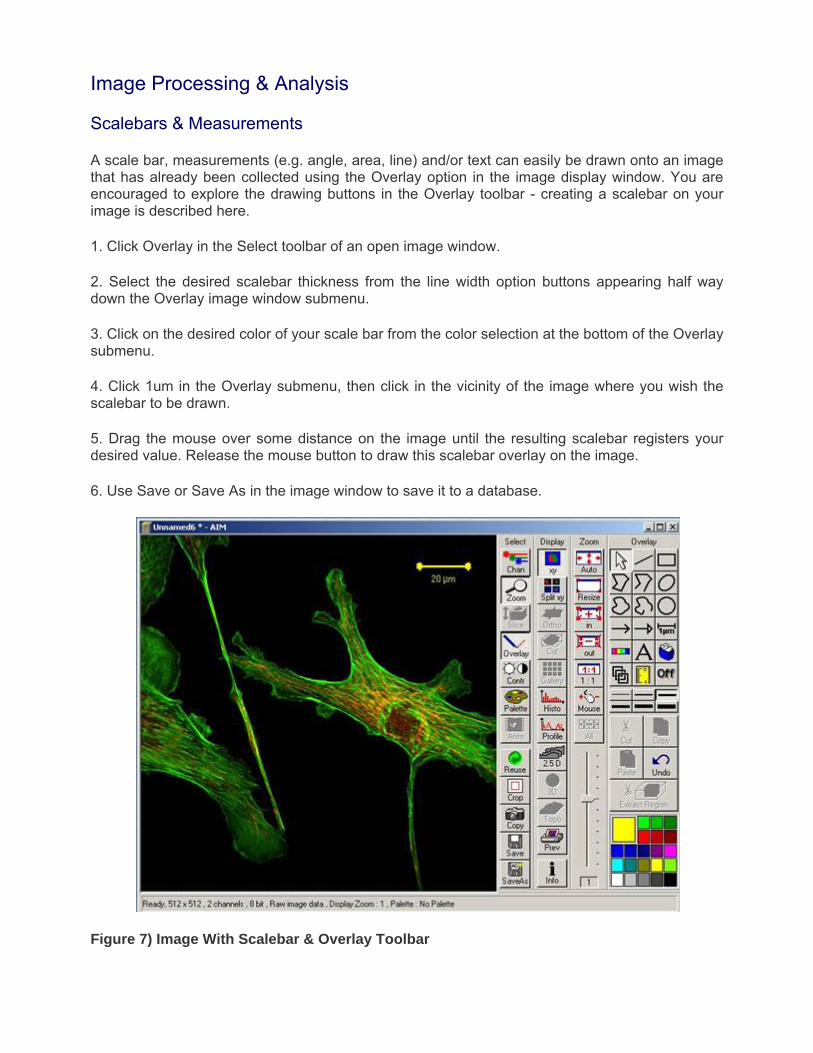
Image Processing & Analysis

Scalebars & Measurements

A scale bar, measurements (e.g. angle, area, line) and/or text can easily be drawn onto an image that has already been collected using the Overlay option in the image display window. You are encouraged to explore the drawing buttons in the Overlay toolbar - creating a scalebar on your image is described here.

1. Click Overlay in the Select toolbar of an open image window.

2. Select the desired scalebar thickness from the line width option buttons appearing half way down the Overlay image window submenu.

3. Click on the desired color of your scale bar from the color selection at the bottom of the Overlay submenu.

4. Click 1um in the Overlay submenu, then click in the vicinity of the image where you wish the scalebar to be drawn.

5. Drag the mouse over some distance on the image until the resulting scalebar registers your desired value. Release the mouse button to draw this scalebar overlay on the image.

6. Use Save or Save As in the image window to save it to a database.

Figure 7) Image With Scalebar & Overlay Toolbar

3-D stack display options

Animate

Some users will find it helpful to assess their time or z-stack data by animating it.

1. Select Anim from the Select toolbar of a stack's "Image" window. The "Animate" window will open and the stack will immediately be animated.

2. Speed 1 and Speed 2 in the bottom section of the "Animate" window allow the user to control the speed of the animation.

3. To further control the animation, use the function buttons in the top section of this window to animate forward and/or in reverse, stop, fast forward, and fast back through a stack. + and - will animate the stack in forward or reverse by whatever increment you choose in the Increment slider in the bottom section of this window.

4. The Increment slider reduces the number of slices included in the animation to every nth slice as selected.

Gallery

Stack slices are organized in rows and presented in the order in which they were generated inside the image window. A 2-dimensional gallery of z-stacks over time can also be generated. Each slice's z-data (um) and/or temporal interval can easily be displayed in every tile of the gallery. Z- or t-galleries can be saved as an image in a database for quick future reference. Additionally, a subset of images within a stack can be selected and stored for later use (e.g. to create a 3-D projection).

1. Click Gallery in the Display toolbar of the image window. A gallery of the entire stack is automatically generated and the Gallery toolbar becomes available in the image window. Click Save if you want to save the gallery to your database for quick future reference. Otherwise, a gallery view can always be generated from the stack at a later time.

2. For z-stacks taken over a time series, refer to the Gallery menu to select the format in which you'd like the gallery be displayed - Z , Time , or entire z-stacks over time, Z + Time .

3. To have the stack data (z distance or time interval) displayed in every tile of the gallery, click Data in the Gallery toolbar. Use the color selection button (located below Data ) to ascribe a color of your choice to the gallery data display.

4. To separate a subset of images from the full image gallery, select Subset in the Gallery toolbar. Here, define new start and end points of the series using the Start Slice and End Slice sliders/data fields, or enter a value in the Every n-th Slice field if you would rather create a subset of every n-th slice of your choosing.

3-D Projection

The Projection function can render a single projection or a series of calculated projections at set angle increments around the X, Y, or Z axis. The user can choose between manipulating aspects of the projection's transparency or creating a projection that has maximum intensity.

The "Transparent" projection method decreases the brightness of each file in the projected stack to reveal structure in subsequent layers that would otherwise be hidden. The "Maximum" projection method takes the intensity values of individual pixels in all sections and collapses them into one single illuminated image. The "Maximum" method is chosen when the maximum pixel intensity is desired to be represented in the projection.

Creating a maximum projection is described here. These instructions assume that an image stack is open and therefore available for projection.

1. Select 3D View → Projection from the main menu. The Projection window will open.

2. Select the stack to be projected in the Source panel of this window.

Only stacks and images that are currently open are available for selection in the Source pulldown list.

3. To create an en face (straight-on) projection of all slices in the z-axis, select the Y radiobutton in the Projection panel. Leave the First Angle set to 0 degrees, enter 1 in the Number Projections field, and set the Difference Angle field to 0 degrees.

4. In the Transparency tab, select the Maximum radiobutton.

5. Generate the projection by clicking Apply located in the upper right corner of the Projection window.

The projection calculation can be monitored via the progress toolbar at the bottom of the image window.

6. If a sequence of projections at set angles has been created, it may be animated or viewed in a gallery via the Select and Display toolbars of the image window.

Exporting Files to .tif Format

Files can be exported in a couple of different ways - via the batch export macro, which allows the simultaneous export of multiple database items or the Export of Images function, which allows the export of individual database items - be they single confocal sections or a stack. The Export of Images method is described here.

1. Open your database and load (open) the file you would like to export.

2. Select File >Export from the main menu. The "Export Images and Data" window will open.

3. In the Save In field, designate to which drive or directory the exported data should be saved.

4. Enter a name for the exported image or series of images in the File name field.

5. In the Save as type field, select the image format into which the file should be exported.

When selecting an image format, pay heed to whether you are exporting a single confocal image or a series (stack) of confocal images. Various image formats are supported (e.g. .bmp, .jpg), we recommend TIF (.tif) format as it is lossless and widely usable.

For multi-channel images, you have the option of exporting individual color channels of data in monochrome (grayscale) if Raw data single or Raw data series image type is chosen.

6. Click Save.

When a z- or time stack file is exported, each stack slice is stored as an individual TIF image with a 3-digit numbered suffix appended to the designated file name.

Assigning Macros To Buttons In Macro Control

1. Open the software and click Macro main menu item.

2. Select Macro that now appears in the bottom right corner of the main menu toolbar. This opens the Macro Control window.

3. Click on the Assign Macro to Button panel.

4. Indicate which button you want the new macro assigned (Button1, Button2, Button3, etc) from the drop down menu in the Button field.

5. Name the new button in the Text field.

6. Click the ... button beside the Project field to link a macro of your choice to the newly created button. An Open window appears. All macro programs can be found in the C:AIM\Macros folder.

7. Find the macro file that you want to load. Select this file and click on Ok in the Open window.

8. Select the macro name from the drop down menu of the Macros field.

9. Hit Apply and the macro you selected should be assigned to the button you designated in step 4. In a moment, the specified button will appear in the Macro toolbar.

Deleting A Macro From A Button In Macro Control

1. Working under the Macro main menu item, select Macro that appears in the bottom right corner of the main menu toolbar. This opens the Macro Control window.

2. Click on the Assign Macro to Button panel.

3. Choose which button you want to disassociate from its macro in the drop down menu in the Button field.

4. Press Delete to delete the linking of the macro program to the button. The specified button should then ghost out to a blank n.n format.

Initializing User Software Settings - Running Registry Files

1. Logon to the system using your ASADMIN user name and password.

2. Run all the registry files in the folder on the desktop:

Double-click each of the files, after each file, you should see a dialog box confirming the registry has been successfully updated. Click "OK" to these messages. You will need to rerun LSM-Macros.reg whenever you want to use a newly installed macro (e.g. newer version of multitime).

3. Start the LSM510 software as normal - "Scan New Image" & "Start Expert Mode"

4. In the Options menu, click the Settings submenu. Make the following settings in the different tabbed sections of this submenu.

Program Start:

- Select FITC (Cy2) from the pull down list or whatever configuration you wish the software to load by default every time you log on. - Un-select "don't show logo"

Save:

- Select the third radio button - at "Create Database" automatically create a subdirectory with the same name as specified database and create dataset image files in that subdirectory.

Temporary Files:

"Use RAM" is fine unless you're doing time lapse, then you may want to set a temporary location, e.g. to your server directory:

Import/Export:

Set location of files; click "User Default Path" to use your default directory defined by your user profile

Record/Reuse:

Check all but objective