arX

iv:m

ath.

DG

/040

6111

v1

7 J

un 2

004

On geodesic equivalence of Riemannian metrics and

sub-Riemannian metrics on distributions of corank 1

Igor Zelenko∗

Abstract

The present paper is devoted to the problem of (local) geodesic equivalence of Riemannianmetrics and sub-Riemannian metrics on generic corank 1 distributions. Using PontryaginMaximum Principle, we treat Riemannian and sub-Riemannian cases in an unified way andobtain some algebraic necessary conditions for the geodesic equivalence of (sub-)Riemannianmetrics. In this way first we obtain a new elementary proof of classical Levi-Civita’s The-orem about the classification of all Riemannian geodesically equivalent metrics in a neigh-borhood of so-called regular (stable) point w.r.t. these metrics. Secondly we prove thatsub-Riemannian metrics on contact distributions are geodesically equivalent iff they are con-stantly proportional. Then we describe all geodesically equivalent sub-Riemannian metricson quasi-contact distributions. Finally we make the classification of all pairs of geodesicallyequivalent Riemannian metrics on a surface, which proportional in an isolated point. Thisis the simplest case, which was not covered by Levi-Civita’s Theorem.

1 Introduction

Let us recall that two Riemannian metrics on a manifold M are called geodesically (or projec-tive) equivalent at a point q0 ∈M , if in some neighborhood of q0 all their geodesics, consideredas unparametrized curves, coincide. The notion of geodesic equivalence can be generalized di-rectly to sub-Riemannian metrics by replacing Riemannian geodesics by normal sub-Riemanniangeodesics:

Let D be a bracket-generating (completely nonholonomic) distribution on M . A Lipschitziancurve ξ(t) is called admissible for the distribution D, if it is tangent to D almost everywhere,i.e., ξ(t) ∈ D

(

ξ(t))

a.e.. A sub-Riemannian metric G on D is given by choosing an inner product

Gq(·, ·) on each subspaces D(q) for any q ∈ M smoothly w.r.t. q. Let || · ||q =√

Gq(·, ·) bethe corresponding Euclidean norm on D(q). For any admissible curve ξ : [0, T ] 7→M its length

w.r.t. the sub-Riemannian metric G is equal to∫ T0 ||ξ(t)||ξ(t) dt. Given two points q1 and q2 one

can look for the curve of minimal length among all admissible curves connecting q1 with q2. Thisproblem can be obviously reformulated as a time-minimal control problem (for this one takesinto the consideration only admissible curves parametrized by the length). The sub-Riemannianextremal trajectory w.r.t. the metric G is the projection to M of a Pontryagin extremal of thisproblem (which lives in the cotangent bundle T ∗M).

In general, Pontryagin extremals can be normal or abnormal: the extremal is called ab-normal, if the Lagrange multiplier of the functional is equal to zero, and normal otherwise.The projection of normal (abnormal) Pontryagin extremal is called a normal (abnormal) sub-Riemannian extremal trajectory. Any abnormal sub-Riemannian extremal trajectory, considered

∗S.I.S.S.A., Via Beirut 2-4, 34014, Trieste, Italy; email: zelenko@sissa.it

1

as unparametrized curves, is characterized by distribution D only, but not by the metric on it.Normal sub-Riemannian extremals surely depend on the metric. They can be described in thefollowing simple way: Let h : T ∗M 7→ R satisfies

h(p, q) =1

2

(

maxp(v) : ||v||q = 1, v ∈ D(q))2

q ∈M, p ∈ T ∗q M. (1.1)

Then the normal sub-Riemannian extremal trajectories are exactly the projections on M of thetrajectories of the Hamiltonian system λ = ~h(λ), lying on the 1

2 -level set of h, i.e., on the setλ ∈ T ∗M : h(λ) = 1

2.

Remark 1 The norm || · ||q on Dq induces the norm on the dual space, which will be denotedalso by || · ||q. Therefore taking the restriction p|D(q) of some covector p ∈ T ∗

q M one can rewrite(1.1) in the following form

h(p, q) =1

2||p|D(q)||2q q ∈M, p ∈ T ∗

q M. (1.2)

Note that a Riemannian metric is actually the sub-Riemannian metric with D = TM andclassical Riemannian geodesics are exactly normal extremal trajectories in this situation (hereabnormal extremals do not exist). Note also that, as in Riemannian case, sufficiently small piecesof normal sub-Riemannian extremal trajectories are length minimizers (see, for example, [5],Appendix C there). Therefore we will call them in the sequel normal sub-Riemannian geodesics.The following definition is a natural extension of the notion of the geodesic equivalence fromRiemannian to the general sub-Riemannian case:

Definition 1 Two sub-Riemannian metrics given on a distribution D of a manifold M arecalled geodesically (or projective) equivalent at a point q0 ∈M , if in some neighborhood of q0 alltheir normal geodesics, considered as unparametrized curves, coincide.

It is clear that if sub-Riemannian metrics G1 and G2 are constantly proportional, i.e., thereexists a positive constant C such that G2q = CG2q for any q, then they are geodesically equiv-alent. The first appearing question is whether there exist constantly non-proportional geodesi-cally equivalent sub-Riemannian metrics? The simplest example of constantly non-proportionalRiemannian metrics on a surface can be described as follows: Let P and S be a plane and ahemisphere in R

3 such that equator of the hemisphere is parallel to the plane. Let G1 and G2

be the metrics on P and S respectively, induced from the Euclidean metric on R3. Denote by

F : S 7→ P the stereographic projection from the center O of the hemisphere (namely, if q ∈ Sthen F (q) is the only point on P lying on the straight line, which connects O and q). Thenthe mapping F sends geodesics of G2 (arcs of big circles on S) to geodesics of G1 (straightlines on P ). Therefore G1 is geodesically equivalent to G2 = (F−1)∗G2, the pull-back of G2 byF−1, but this metric are not constantly proportional. Moreover, as E. Beltrami showed in [1],a Riemannian metric on a surface is geodesically equivalent to the flat one iff it has a constantcurvature.

Let us introduced some notions, which are important for the considered problem. For a givenordered pair of sub-Riemannian metrics G1, G2 and a point q one can define the following linearoperator Sq : D(q) 7→ D(q):

G2q(v1, v2) = G1q(Sqv1, v2), v1, v2 ∈ D(q).

Obviously, Sq is self-adjoint w.r.t. the Euclidean structure given by G1.

2

Definition 2 The operator Sq will be called the transition operator from the metric G1 tothe metric G2 at the point q.

Let N(q) be the number of distinct eigenvalues of the operator Sq.

Definition 3 The point q0 is called regular w.r.t. the pair of sub-Riemannian metrics G1

and G2, if the function N(q) is constant in some neighborhood of q0.

Note that the regularity of the point q0 is equivalent to the fact that the set of multiplicitiesof eigenvalues of the transition operator Sq is the same for all points q from some neighborhoodof q0 (in [7] regular points were called stable). By standard arguments one can show that thefunction N(q) is lower semicontinuous. This together with the fact that it is integer-valuedimplies the following

Proposition 1 The set of regular points w.r.t. the pair of sub-Riemannian metrics is openand dense in M .

For Riemannian metrics on an n-dimensional manifold all possible pairs of geodesically equiv-alent metrics in a neighborhood of a regular point w.r.t. these metrics were described already byLevi-Civita in [4] (see Theorem 1 below and also [7]), who had extended the earlier result of Dinifor surfaces (see [2],[3], or [6]) to an arbitrary n. From this result it follows that Riemannianmetrics, for which there exists at least one non-proportional geodesically equivalent Riemannianmetric, are of the very special form.

The classification of geodesically equivalent Riemannian metrics at non-regular points (i.e.,points, where eigenvalues of transition operator bifurcate) even on a surface was not done,while the geodesic equivalence of proper sub-Riemannian metrics (i.e, when D 6= TM and D isbracket-generating) was not studied before. In the present paper we treat both these problems.

In the sequel for shortness (m,n)-distribution means an m-dimensional subbundle of thetangent bundle of an n-dimensional manifold. Our study of the geodesic equivalence of propersub-Riemannian metrics will be mainly concentrated on the following two cases:

1. D is the contact distribution. Namely, D is a corank 1 distribution on an odd dimensionalmanifold such that if ω is a differential 1-form, which annihilates D, D(q) = v ∈ TqM :ωq(v) = 0, then the restriction dω|D of the differential dω on D is a nondegenerated2-form at any q. In this case there are no abnormal Pontryagin extremals.

2. D is the quasi-contact distribution. Namely, D is a corank 1 distribution on an evendimensional manifold such that if ω is a differential 1-form, which annihilates D, thenthe restriction dω|D of the differential dω on D has 1-dimensional kernel at any q. Thekernels of dω|D form line distribution. We will call it the abnormal line distribution ofthe quasi-contact distribution D. Abnormal extremal trajectories of the sub-Riemannianmetric G on D are exactly the leaves of this distribution, parametrized by the length.

Clearly in both cases the germs of distribution D are generic germs of corank 1 distributions.Note also that in both cases there exists only one, up to a diffeomorphism, distribution satisfyingthe prescribed properties (a particular case of Darboux’s Theorem). Actually, our methodworks for sub-Riemannian metrics defined on much more general distributions, for example,on so-called step 1 bracket-generating distributions: an (m,n)-distribution D is called step 1bracket-generating if dimDl+1 = dimDl + 1 for any 1 ≤ l ≤ n −m (here the lth power Dl ofthe distribution D is defined by induction Dl = Dl−1 + [D,Dl−1]). The study of the problem

3

of the geodesic equivalence for sub-Riemannian metrics on general step 1 bracket-generatingdistributions will be done in our future publications.

The paper is organized as follows. In section 2 we show that the problem of geodesic equiv-alence of sub-Riemannian metrics can be reduced to the question of the existence of an orbitaldiffeomorphism between the corresponding flows of extremals. This reduction is obvious in theRiemannian case, but in the proper sub-Riemannian case it has some additional difficulties,especially in the presence of abnormal extremals. After this reduction we express the conditionfor the existence of the orbital diffeomorphism in terms of the special frame adapted to thepair of sub-Riemannian metrics. Further for step 1 bracket-generating distributions we obtaina necessary condition for the geodesic equivalence in terms of divisibility of some polynomials(on the fibers of the cotangent bundle of the ambient manifold) associated with these metrics.We call it the first divisibility condition. It imposes rather strong restrictions on the pair of themetrics.

In section 3 we give the coordinate-free formulation of Levi-Civita’s Theorem (Theorem 1)and prove it in a new, rather elementary way, using the conditions for the existence of theorbital diffeomorphism and the first divisibility condition. In section 4 for a sub-Riemannianmetric on corank 1 distribution we obtain an additional necessary condition for the geodesicequivalence in terms of divisibility of some polynomials associated with these metrics. Wecall it the second divisibility condition. Using the conditions for the existence of the orbitaldiffeomorphism and the second divisibility condition we prove that sub-Riemannian metrics oncontact distributions are geodesically equivalent iff they are constantly proportional (Theorem2) and we give the classification of all geodesically equivalent sub-Riemannian metrics on quasi-contact distributions (Theorem 3). This classification is given in coordinate-free way and hasapparent similarities with our interpretation of Levi-Civita’s Theorem. This gives a hope forthe existence of a general classification theorem about geodesic equivalence of sub-Riemannianmetrics defined on very general class of distribution, which will contain as particular cases thecases considered in the present paper.

Finally in section 5 for the Riemannian metrics on a surface we obtain the classification ofgeodesically equivalent pairs at a non-regular point (the point of bifurcation of the eigenvaluesof the transition operator). Note that for generic pair of Riemannian metrics on a surfacethe set of points of their proportionality consists of isolated points. Therefore it is natural toconsider the case when two Riemannian metrics on a surface are proportional in an isolatedpoint. Some results of the global topological nature (namely, about the number of the points ofproportionality for a pair of globally geodesically equivalent Riemannian metrics on a sphere)were obtained in [6], but the local classification surprisingly was not done before. The canonicalconformal structure on a surface, associated with a Riemannian metric, plays the crucial role inthis classification. Using this conformal structure and Dini’s Theorem (Levi-Civita’s Theorem inthe case of a surface), one can associate any pair of geodesically equivalent metrics on a surface,which are proportional in an isolated point q0, with some (multiple-valued) analytic functionin a neighborhood of q0 with a singularity at q0. The analysis of this singularity gives us therequired classification (Theorems 5 and 6).

2 Geodesic equivalence and orbital diffeomorphism of the ex-

tremal flows

2.1 Existence of the orbital diffeomorphism Let G1 and G2 be two sub-Riemannianmetrics on a distribution D of a manifold M , || · ||1q and || · ||2q be the corresponding Euclidean

4

norms on D(q), h1 and h2 be the Hamiltonians, defined by (1.1), where || · ||q is replaced by|| · ||iq, i = 1, 2. Also let H1 and H2 be the 1

2 -level sets of h1 and h2 respectively, i.e.

Hi = λ ∈ T ∗M : hi(λ) =1

2. (2.1)

Besides, for given distribution D and metric G on it denote by Jk(D,G) the space of k-jets ofall Ck curves admissible to D and parametrized by length w.r.t. the metrics G. By definitionthe 1-jet J1(D,G) satisfies

J1(D,G) = (q, v) : q ∈M,v ∈ D(q), ||v||q = 1.

For given curve γ we will denote by j(k)t0 γ the k-jet of the curve γ at the point t0.

Proposition 2 If for some neighborhood U of q0 in M there exist a fiberwise diffeomorphismΦ : H1 ∩ T ∗U 7→ H2 ∩ T ∗U and a function a : H1 7→ R such that

Φ∗~h1(λ) = a(λ)~h2

(

Φ(λ))

, (2.2)

then the metrics G1 and G2 are geodesically equivalent at q0.

Proof. Indeed, Φ maps any trajectory of the system λ = ~h1(λ), lying in H1 ∩ T ∗U , tothe curve, which coincides, up to reparametrization, with a trajectory of the system λ = ~h2(λ).Therefore in U any normal sub-Riemannian geodesics of G1 is, up to reparametrization, a normalsub-Riemannian geodesics of G2.

In the case of Riemannian metrics the relation (2.2) is also necessary for the geodesic equiv-alence of metrics G1 and G2. Indeed, in this case there is only one geodesic passing through the

given point in the given direction, and the map P(1)i : Hi 7→ J1(TM,Gi) defined by

Pi(λ)def= j10π(et

~hi) =(

π(λ), π∗(

~hi(λ))

)

, i = 1, 2, (2.3)

is a diffeomorphism (here we denote by π : T ∗M 7→M the canonical projection and by et~hi the

flow generated by vector field ~hi, i = 1, 2). So, directly by definition, if the metrics G1 and G2

are geodesically equivalent at q0, then there is a neighborhood U of q0 such that the followingdiffeomorphism

Φ(λ) =(

P 12

)−1

(

1

||P 11 (λ)||2q

P 11 (λ)

)

, q = π(λ), (2.4)

is fiberwise, maps H1 ∩ T ∗U to H2 ∩ T ∗U and satisfies (2.2) on H1 ∩ T ∗U .

Definition 4 A fiberwise diffeomorphism Φ defined on a nonempty open set B of H1 suchthat Φ(B) ⊂ H2 is called the orbital diffeomorphism of the extremal flows of the sub-Riemannianmetrics G1 and G2 on B, if it satisfies (2.2) for any λ ∈ B.

Let us study the question, whether the existence of the orbital diffeomorphism is necessaryfor the geodesic equivalence of sub-Riemannian metrics. In the case of a proper sub-Riemannianmetric (i.e., D 6= TM , D is bracket-generating) an entire family of normal sub-Riemanniangeodesics passes in general through the given point in the given direction. So, in order todistinguish different normal geodesics, passing through a point, we need jets of higher order.Besides, the presence of the abnormal extremal trajectories causes to addition difficulties, as

5

shown below. By analogy with (2.3) let us define the following mapping P(k)i : Hi 7→ Jk(D,Gi),

i = 1, 2:

P(k)i (λ)

def= jk0π(et

~h) (2.5)

Then one can check without difficulties that:a) if D is contact then the mapping P

(2)i establishes the diffeomorphism between Hi and its

image;b) if D is quasi-contact, C is the abnormal line distribution of D, and the set Si ⊂ Hi is

defined bySi = λ ∈ Hi : P 1

i (λ) ∈ C, (2.6)

then the restriction of the mapping P(2)i on Hiq\Si establishes the diffeomorphism between

Hiq\Si and its image, while the restriction of P(2)i on Si is constant on each fiber.

Now denote by Ωq(D,Gi) the set of all C∞ admissible curves, starting at q and parametrizedby length w.r.t. the metric Gi and let Jk

q (D,Gi) be the space of k-jet of these curves at 0.Consider the mapping Iq : Ωq(D,G1) 7→ Ωq(D,G2) which sends a curve γ to its reparametriza-

tion (w.r.t. the length of G2). Obviously , this mapping induces the diffeomorphisms I(k)q :

Jkq (D,G1) 7→ Jk

q (D,G2). Collecting all such diffeomorphisms for any q we obtain a diffeomor-

phism I(k) : Jk(D,G1) 7→ Jk(D,G2). Then similarly to (2.4) we obtain that if the distributionD is one of the two listed in Introduction, and the sub-Riemannian metrics G1 and G2, definedon D, are geodesically equivalent at q0, then there exist a neighborhood U of q0 such that thefollowing mapping

Φ(λ) =(

P(2)2

)−1 I(2) P (2)1 (λ), (2.7)

is well defined on the set B, where B = H1 ∩ T ∗U in contact case and B = (H1 ∩ T ∗U)\S1 inquasi-contact (here S1 is as in (2.6)). Moreover, such Φ is the orbital diffeomorphism on the setB w.r.t. the metrics G1 and G2. We have proved the following

Proposition 3 If G1 and G2 are Riemannian metric or sub-Riemannian metrics definedon contact or quasi-contact distributions and if they are geodesically equivalent at some pointq0, then for some neighborhood U of q0 there exists the orbital diffeomorphism of the extremalflows of the metrics G1 and G2 on some nonempty open set B in H1 ∩ T ∗U , π(B) = U . In theRiemannian and contact case one can take B = H1 ∩ T ∗U , while in quasi-contact case one cantake B = (H1 ∩ T ∗U)\S1, where S1 is as in (2.6).

Actually, there is an analogue of the previous proposition for sub-Riemannian metrics definedon much more wide class of distributions. To formulate it let us introduce some notations.Denote by Aq0

(D) the set of all points q ∈ M which can be connected with q0 by abnormalextremal trajectory of the distribution D. For example, in Riemannian and contact case Aq0

(D)is empty; in quasi-contact case Aq0

(D) is the set Lq0\q0, where Lq0

is the leaf of the abnormalline distribution, passing through q0.

Proposition 4 Suppose that the sub-Riemannian metrics G1 and G2, defined on the bracket-generating distribution D, are geodesically equivalent at the point q0 and for any neighborhoodV of q0 the set V \Aq0

(D) has positive Lebesgue measure. Then for some neighborhood U of q0there exists the orbital diffeomorphism of the extremal flows of the metrics G1 and G2 on someopen set B in H1 ∩ T ∗U , π(B) = U .

Remark 2 Actually in the previous proposition one can replace the set Aq0(D) by the set of

all points q ∈M which can be connected by abnormal extremal trajectory, having minimal lengthw.r.t. the metric G1 (or G2) among all admissible trajectories with endpoints q0 and q.

6

Since in the present paper we solve completely the problem of geodesic equivalence only inthe cases, considered in Proposition 3, we postpone the proof of Proposition 4 and the statementin Remark 2 to the future paper.

2.2 The orbital diffeomorphism in terms of the adapted frame to the pair ofmetrics. Suppose that D is an (m,n)-distribution on a manifold M . Let q0 be a regular pointw.r.t. the metric G1 and G2 (see Definition 3). It is simple to show that the regularity ofthe point q0 is equivalent to the fact that the set of the multiplicities of the eigenvalues of thetransition operator Sq is the same for all points q from some neighborhood of q0. Thereforein some neighborhood U of q0 one can choose the basis (X1, . . . ,Xm) of the distribution Dorthonormal w.r.t. the metric G1 such that each Xi(q) is eigenvector of the transition operatorSq, q ∈ V . Such basis of D will be called the adapted basis to the ordered pair of metrics(G1, G2) on a set U . A frame (X1, . . . ,Xn) will be called the adapted frame to the ordered pairof sub-Riemannian metrics (G1, G2) on a set U , if the tuple

(

X1, . . . ,Xm) is the adapted basisof D w.r.t. (G1, G2) on U .

Let us express the relation (2.2) for the orbital diffeomorphism in terms of some adaptedframe (X1, . . . ,Xn) . Let ui : T ∗M 7→ R be the ”quasi-impulse” of the vector field Xi,

ui(p, q) = p(

Xi(q))

, q ∈ U, p ∈ T ∗U. (2.8)

For given diffeomorphism Φ defined on an open set of T ∗M denote by

Φi = ui Φ, 1 ≤ i ≤ n. (2.9)

Suppose also that for any i, 1 ≤ i ≤ m, the eigenvalue of the transition operator Sq, correspond-ing to the eigenvector Xi(q), is equal to α2

i (q).

Lemma 1 If Φ is the orbital diffeomorphism of the extremal flows of the metrics G1 andG2 on an open set B ⊂ H1 ∩ T ∗U , then the functions Φi with 1 ≤ i ≤ m satisfy

Φi =α2

i ui√

∑mk=1 α

2ku

2k

, 1 ≤ i ≤ m. (2.10)

Proof. Since by construction the tuple (X1, . . . ,Xm) constitute an orthonormal basis of thedistribution D w.r.t. the metric G1, the Hamiltonian h1 satisfies h1 = 1

2

∑mi=1 u

2i , and

~h1 =

m∑

i=1

ui~ui, π∗~h1 =

m∑

i=1

uiXi, H1 =

λ ∈ T ∗U :

m∑

i=1

u2i = 1

(2.11)

(here π : T ∗M 7→M is the canonical projection). Let Xi be

Xi =1

αiXi, 1 ≤ i ≤ m, (2.12)

and ui(p, q) = p(

Xi(q))

be the corresponding quasi-impulses. Then

ui =ui

αi, 1 ≤ i ≤ m, (2.13)

Note that by construction (X1, . . . , Xn) is the orthonormal basis of D w.r.t. the metric G2.Hence, similarly to (2.11), we have ~h2 =

∑mi=1 ui~ui, which together with (2.12) and (2.13)

implies that

π∗~h2 =

m∑

i=1

ui

α2i

Xi, H2 =

λ ∈ T ∗U :

m∑

i=1

u2i = 1

=

λ ∈ T ∗U :

m∑

i=1

u2i

α2i

= 1

(2.14)

7

Suppose that Φ is the orbital diffeomorphism on some set B, satisfying (2.2) for some functiona. Then by definition Φ(λ) ∈ H2 for any λ ∈ B. This together with (2.9) and (2.14) impliesthat

m∑

i=1

Φ2i

α2i

= 1. (2.15)

Further from the fact that Φ is fiberwise and (2.11) it follows that

(π∗ Φ∗)~h1(λ) = π∗~h1(λ) =

m∑

i=1

uiXi.

On the other hand, (2.9) and (2.14) imply

π∗~h2

(

Φ(λ))

=m∑

i=1

Φi

α2i

Xi.

From the last two relations and (2.2) it follows that

aΦi = α2i ui, 1 ≤ i ≤ m

From this and (2.15) it follows easily that

a =

√

√

√

√

m∑

k=1

α2ku

2k, (2.16)

which implies (2.10).

Now we will find the relation for the remaining components Φi, m + 1 ≤ i ≤ n, of Φ. Letckji be the structural functions of the adapted frame (X1, . . . ,Xn), i.e., the function, satisfying

[Xi,Xj ] =∑

ckjiXk. Let the vector fields Xi, 1 ≤ i ≤ m, satisfy (2.12) and set

Xi = Xi, m+ 1 ≤ i ≤ n. (2.17)

Note that by construction (X1, . . . , Xn) is the adapted frame w.r.t. the ordered pair (G2, G1).Let ckji be the structural functions of the frame (X1, . . . , Xn). The following functions will bevery useful in the sequel together with function a, defined by (2.16):

Rjdef=

1

2~h1(α

2j )uj + α2

j~h1(uj) −

1

2α2

juj

~h1(a2)

a2−

∑

1≤i,k≤m

ckjiαiαjαkuiuk, (2.18)

Qjkdef=

m∑

i=1

ckjiαiui (2.19)

Lemma 2 A map Φ is the orbital diffeomorphism on a set B of the extremal flows of themetrics G1 and G2 iff on B the functions Φk with m+ 1 ≤ k ≤ n satisfy the following relations:

∀1 ≤ j ≤ m : αj

n∑

k=m+1

QjkΦk =Rj

a(2.20)

∀m+ 1 ≤ s ≤ n : ~h1(Φs) −n∑

k=m+1

QskΦk =1

a

m∑

k=1

Qskαkuk. (2.21)

8

Proof. In the sequel we set

∀m+ 1 ≤ n : αi ≡ 1. (2.22)

Denote by Yi the vector field on H1, which is the lift of the vector field Xi (i.e., π∗Yi = Xi),and duj(Yi) = 0 ∀1 ≤ j ≤ n (i.e., Yj is horizontal field of the connection on T ∗M defined bydistribution, satisfying du1 = . . . = dun = 0). Similarly, let Yi be the vector field on H2, which isthe lift of Xi and duj(Yi) = 0 for all 1 ≤ j ≤ n. Note also that the tuple (u1, . . . , un) defines thecoordinates on each fiber T ∗

q M of T ∗M . So, one can define the vector fields ∂ui, 1 ≤ i ≤ n, as

follows: ∂uiis vertical (i.e., tangent to the fibers of T ∗M) and duj(∂ui) = δij for all j = 1, . . . n,

where δij is the Kronecker symbol. In the same way one can define the fields ∂ui. With this

notations, using (2.12) and (2.13), ∀1 ≤ i ≤ n one can easily obtain the following relation :

∂ui= αi∂ui

, Yi =1

αi

Yi +

m∑

j=1

Xj(αi)

αiuj∂uj

(2.23)

Besides, by standard calculations, we have

~h1 =m∑

i=1

ui~ui =m∑

i=1

uiYi +m∑

i=1

n∑

j,k=1

ckjiuiuk∂uj, (2.24)

~h2 =m∑

i=1

ui~ui =m∑

i=1

uiYi +m∑

i=1

m∑

j,k=n

ckjiuiuk∂uj. (2.25)

Substituting (2.13) and (2.23) into (2.25), we obtain

~h2 =

m∑

i=1

ui

α2i

Yi +

m∑

i,j=1

Xi(αj)

α2iαj

uiuj∂uj+

m∑

i=1

n∑

j,k=1

ckjiαj

αiαkuiuk∂uj

. (2.26)

This together with (2.10) implies easily that

~h2

(

Φ(λ))

= a−1m∑

i=1

uiYi + a−2m∑

j=1

(1

2~h1(α

2j )uj +

m∑

i,k=1

ckjiαiαjαkuiuk

)

∂uj+

a−1m∑

j=1

n∑

k=m+1

m∑

i=1

ckjiαiαjuiΦk∂uj+

n∑

s=m+1

m∑

i=1

(

a−2m∑

k=1

cksiαiαkuiuk+ (2.27)

a−1n∑

k=m+1

cksiαiuiΦk

)

∂us , (2.28)

where a is as in (2.16). On the other hand, from the fact that Φ is fiberwise and relation (2.10)it follows that

Φ∗~h1(λ) =

m∑

i=1

uiYi +

m∑

j=1

~h

α2juj

√

∑ml=1 α

2l u

2l

∂uj+

n∑

j=m+1

~h(Φj)∂uj. (2.29)

Using relations (2.27) and (2.29), it is not hard to check by direct calculations that (2.2) holdsiff both (2.20) and (2.21) hold, which concludes the proof of the Lemma.

9

2.3 The first divisibility condition. Let I1 : D(q)∗ 7→ D(q) be the canonical isomorphismw.r.t. the inner product G1q(·, ·), namely, ℓ(·) = G1q(I1(ℓ), ·) ∀ℓ ∈ D(q)∗. Define the followingfunction P : T ∗M 7→ R:

P(p, q) =(

||I1(p|D(q))||2q

)2, q ∈M,p ∈ T ∗

q M (2.30)

(here || · ||2q is the Euclidean norm on D(q) corresponding to the inner product G2q(·, ·), p|D(q)

is the restriction of covector p ∈ T ∗q M on the subspace D(q)). Obviously, the restriction of P on

each fiber T ∗q M is a degree 2 homogeneous polynomial, while the restriction of ~h1(P) on each

fiber T ∗q M is a degree 3 polynomial. Besides, in a neighborhood of the regular point

P = a2 =

m∑

i=1

α2i u

2i , (2.31)

where (u1, . . . , um) are quasi-impulses of the vectors of the adapted basis (X1, . . . Xm) to theorder pair (G1, G2) and α2

i are eigenvalues of the transition operator Sq, corresponding to theeigenvectors Xi.

Definition 5 We will say that the ordered pair (G1, G2) of sub-Riemannian metrics on thedistribution D satisfies the first divisibility condition on a set U , if the polynomial ~h1(P)|T ∗

q M isdivided by the polynomial P|T ∗

q M for any q ∈ U .

Proposition 5 Let D be an (m,n)-distribution on a manifold M such that

∀1 ≤ s ≤ n−m+ 1, dimDs = m+ s− 1. (2.32)

Suppose also that for given two sub-Riemannian metrics G1 and G2 on D and for some openset U of M there exists an orbital diffeomorphism of the extremal flows of these metrics in someopen set B in H1∩T ∗U , π(B) = U . Then the pair (G1, G2) satisfies the first divisibility conditionon U .

Proof. Since the set of regular points is dense ( Proposition 1) it is sufficient to prove thefirst divisibility condition for a regular point q0 w.r.t. the pair (G1, G2). Therefore in order toobtain the first divisibility condition we can use Lemmas 1 and 2. Note also that by (2.18) thefunction Rj has the following form on each fiber:

Rj = −1

2α2

juj

~h1(P)

P + polynomial (2.33)

First suppose that D = TM (in this case the assumption (2.32) holds automatically). Thenthe identity (2.20) is equivalent to the identity Rj ≡ 0, 1 ≤ j ≤ n, which holds on open set Bin H1 ∩ T ∗U with π(B) = U and therefore on the whole T ∗U . Hence from (2.33) it follows that

ujh1(P)P

, has to be a polynomial, which implies easily that the polynomial P has to divide the

polynomial ~h1(P), i.e., the first divisibility condition holds.

Now consider the case D 6= TM . By assumption (2.32), we can complete the adapted basis(X1, . . . ,Xm) to the adapted frame such that

∀m+ 1 ≤ s ≤ n Xs ∈ Ds−m+1 (2.34)

10

Then D2 = span(X1, . . . Xm+1), which implies that there exist indices i, j, 1 ≤ i, j ≤ m, suchthat cm+1

j i(q0) 6= 0, while ckij = 0 for all 1 ≤ i, j ≤ m and k > m+ 1. In other words,

∀k, j : k > m+ 1, 1 ≤ j ≤ m Qjk ≡ 0 (2.35)

∃j : 1 ≤ j ≤ m, Qjm+1 6≡ 0 (2.36)

(see (2.19) for the definition of the functions Qjk). Then from (2.20) it follows that

Φm+1 =Rj

αjQjm+1

√P. (2.37)

Using (2.33), we obtain

Φm+1 = −1

2αjuj

~h1(P)

Qjm+1P3/2+

1

αjQjm+1

√P

polynomial (2.38)

on each set B ∩ T ∗q M , q ∈ U .

Further, from assumption (2.32) it follows that ck+1si = 0 for any k, s, i such that m < s < k

and 1 ≤ i ≤ m. On the other hand, there exist i, 1 ≤ i ≤ m, such that cs+1si

6= 0. In other words,

∀k, s : m < s < k Qs k+1 ≡ 0 (2.39)

∀s : m < s < n− 1 Qs s+1 6≡ 0. (2.40)

Hence by (2.21), applied for s = m+ l − 1 with 2 ≤ l ≤ n−m, one has

Φm+l = Q−1m+l−1 m+l

(

~h1(Φm+l−1) −m+l−1∑

k=m+1

Qm+l−1kΦk − P−1/2m∑

k=1

Qm+l−1,kαkuk

)

. (2.41)

Then by induction from (2.38) and (2.41) it is not difficult to get the following relation for any2 ≤ l ≤ m− n

Φm+l =(−1)l(2l − 1)!!αjuj

(

~h1(P))l

2lQj m+1P l+1/2∏l−1

i=1Qm+i m+i+1

+polynomial

Qlj m+1

P l−1/2∏l−1

i=1Ql−im+i m+i+1

(2.42)

on each B ∩ T ∗q M , q ∈ U . Substituting the expression for Φm+l from (2.42) to identity (2.21)

with s = n one can obtain without difficulties that

uj

(

~h1(P))n−m+1

Qj m+1Pn−m+3/2∏n−m−1

i=1 Qm+i m+i+1

=polynomial

Qn−m+1j m+1

Pn−m+1/2∏n−m−1

i=1 Qn−m−i+1m+i m+i+1

(2.43)

or, equivalently

ujQn−mj m+1

(∏n−m−1

i=1 Qn−m−im+i m+i+1

)(

~h1(P))n−m+1

P = polynomial. (2.44)

on each set B ∩ T ∗q M , q ∈ U . Note that the left-hand side of (2.44) is rational function. Hence

from (2.44) it has to be polynomial. Note also that P is positive definite quadratic form (see(2.31)), while the functions Qjk are linear (with real coefficients) on each fiber. Therefore from

(2.44) it follows easily that the polynomial P has to divide the polynomial ~h1(P), i.e., the firstdivisibility condition holds. The proof of the proposition is concluded. .

Note that if D is contact, quasi-contact, or D = TM , then the assumption (2.32) of theprevious proposition holds. So, as a direct consequence of Proposition 3 and the previousproposition, we have the following

11

Corollary 1 Suppose that two metrics G1 and G2 defined on the distribution D are geodesi-cally equivalent at the point q0. Assume also that the distribution D satisfies one of the twofollowing conditions:

1. D = TM (the Riemannian case);

2. D is corank 1 contact or quasi-contact distribution;

Then the pair (G1, G2) satisfies the first divisibility condition on U .

So, in the cases under consideration the first divisibility condition is necessary for the geodesicequivalence. In the next proposition we collect all information from the first divisibility condition,which will be used in the sequel. It shows that the first divisibility condition imposes ratherstrong restrictions on the pair of the metrics.

Proposition 6 Suppose that the metrics G1 and G2, defined on the distribution D, satisfythe first divisibility condition on some set U . If (X1, . . . Xm) is a basis of D adapted to the orderpair (G1, G2), and the transition operator Sq has the form Sq = diag (α2

1(q), . . . , α2m(q)) in this

basis (αi > 0), then the following relations hold

[Xi,Xj ](q) /∈ D(q) ⇒ αi(q) = αj(q); (2.45)

Xi

(

α2j

α2i

)

= 2cjji

(

1 −α2

j

α2i

)

; (2.46)

Xi

(

α2j

αi

)

= 0, αi 6= αj (2.47)

Xi

(

αj

αk

)

= 0, αj 6= αi, αk 6= αi; (2.48)

(α2j − α2

i )ckji + (α2

j − α2k)c

ijk + (α2

i − α2k)c

jik = 0, i, j, k are pairwise distinct. (2.49)

(in all relations above 1 ≤ i, j, k ≤ m).

Proof. As before let us complete the adapted basis (X1, . . . Xm) of D somehow to the localframe. From (2.24) and (2.31) by direct calculation one has

~h1(P) =m∑

i,j=1

Xi(α2j )uiu

2j + 2

m∑

i,j=1

n∑

k=1

ckjiα2juiujuk (2.50)

On the other hand by the first divisibility condition there exist functions pi(q), 1 ≤ i ≤ n, suchthat

~h1(P) =(

n∑

i=1

piui

)(

m∑

j=1

α2ju

2j

)

. (2.51)

Relation (2.49) follows immediately from comparing the coefficients of uiujuk in the right-hand sides of (2.50) and (2.51), where i, j, k are pairwise distinct and 1 ≤ i, j, k ≤ m.

Further, comparing the coefficient of uiujuk in the right-hand side of (2.50)and (2.51), where1 ≤ i ≤ j ≤ m and k > m, we have

ckji(α2i − α2

j ) = 0 (2.52)

12

Therefore, if [Xi,Xj ](q) /∈ D(q), then there exists k > m such that ckji(q) 6= 0, which impliesthat αi(q) = αj(q). Relation (2.45) is proved.

Further, comparing coefficients of u3i in the right-hand sides of (2.50) and (2.51) we obtain

that

pi =Xi(α

2i )

α2i

, (2.53)

while comparing coefficients of uiu2j with i 6= j and using (2.53) one obtains easily that

α2iXi(α

2j ) − α2

jXi(α2i ) = 2cjji(α

2i − α2

j )α2i . (2.54)

The last equation implies (2.46).In order to prove (2.47) note that we can obtain one more relation in addition to (2.46),

starting with the metric G2 as the original one and using transition from the metric G2 to themetric G1. Namely, if Xi is as in (2.12) then by analogy with (2.54) we have

α2i Xi(α

2j ) − α2

j Xi(α2i ) = 2cjji(α

2i − α2

j )α2i . (2.55)

Obviously, αi = 1αi

. Also, by (2.12) one get easily that

cjji =cjjiαi

− Xi(αj)

αiαj. (2.56)

Substituting the last two relations and (2.12) into (2.55) it is not difficult to get the following

α2iXi(α

2j ) − α2

jXi(α2i ) = 2αj

(

(αjcjji −Xi(αj)

)

(α2i − α2

j ) (2.57)

Then combining (2.54) with (2.57) and using the fact that αi 6= αj one get

cjji =1

2

Xi(α2j )

α2j − α2

i

(2.58)

Substituting the last relation again in (2.54) we have

2α2iXi(α

2j ) − α2

jXi(α2i ) = 0,

which is equivalent to (2.47). Relation (2.48) follows immediately from (2.47).

Corollary 2 If D is a bracket-generating (2, n)-distribution, n > 2, and the metrics G1

and G2, defined on D, satisfy the first divisibility condition, then they are proportional, namelyG2q = α(q)G1q .

Proof. Since D is bracket-generating, the set V1 of points q with

dimD2(q) = 3 (2.59)

is open and dense. By Proposition 1 the intersection V2 of this set with the set of all regularpoints w.r.t. the metrics G1 and G2 is also open dense. Therefore it is sufficient to proof thecorollary for the points of V2. From regularity it follows the existence of the adapted frame(X1,X2). So, we can apply the previous proposition. By (2.59), [X1,X2] 6∈ D. Hence from(2.45) it follows that α1 ≡ α2, which completes the proof of the corollary.

Suppose that D is a step 1 bracket-generating (2, n)-distribution (dimDl+1 = dimDl +1 forany 1 ≤ l ≤ n −m). It can be shown easily that D satisfy the assumptions of Proposition 4.Therefore by Propositions 4, 5, and Corollary 2 we have the following

13

Proposition 7 Suppose that two sub-Riemannian metrics G1 and G2 are defined on a step1 bracket-generating (2, n)-distribution, where n > 2. If they are geodesically equivalent at somepoint q0, then they are proportional, namely G2q = α(q)G1q in some neighborhood of q0.

Our conjecture is that the factor α(q) in the previous propoposition has to be constant, butwe can prove it still only in the case n = 3 (see Corollary 5 below). We finish this section withthe following useful lemma

Lemma 3 Suppose that the metrics G1 and G2, defined on an (m,n)-distribution D, satisfythe first divisibility condition at some neighborhood U of a regular point q0. If (X1, . . . Xm) isa basis of D adapted to the order pair (G1, G2), and the transition operator Sq has the formSq = diag (α2

1(q), . . . , α2m(q)) in this basis (αi > 0), then the functions Rj , 1 ≤ j ≤ m, defined

by (2.18), can be written in the following form

Rj =m∑

i=1

(1 − δji)(

(α2j − α2

i )ciji −

Xj(α2i )

2

)

u2i +

m∑

i=1

(1 − δji)α2

i

2α2j

Xi

(α4j

α2i

)

uiuj +

m∑

i=1

m∑

k=1

(1 − δik)(α2j − α2

k)ckjiuiuk + α2

j

m∑

i=1

n∑

k=m+1

ckjiuiuk. (2.60)

(here δij is the Kronecker symbol).

The relation can be obtain without difficulties by substitution of (2.53), (2.56) and the followingobvious identity

cki,j = cki,jαk

αiαji, j, k are pairwise distinct (2.61)

into (2.18).

3 The case of Riemannian metrics near regular point

In the present section, using the technique developed above, we give a new proof of classicalLevi-Civita’s Theorem about the classification of all Riemannian geodesically equivalent metricsin a neighborhood of the regular points w.r.t. these metrics (see [4], [7]). This proof is ratherelementary and transparent from the geometrical point of view. Some crucial ideas of this proofwill be used in the next section for obtaining the corresponding classification for sub-Riemanniangeodesically equivalent metrics on quasi-contact distributions.

Here we prefer the coordinate-free formulation of Levi-Civita’s Theorem, which in our opin-ion clarifies the statement of it. But before let us introduce some notations and prove somepreparatory lemmas.

Let G1 and G2 be Riemannian metrics on an n-dimensional manifold M . Let q0 be a regularpoint w.r.t. these metrics. Suppose that (X1, . . . Xn) is a frame adapted to the order pair(G1, G2) in some neighborhood of q0, and the transition operator Sq from the metric G1 to themetric G2 has the form Sq = diag (α2

1(q), . . . , α2n(q)) in this basis (αi > 0).

Let Rj , 1 ≤ j ≤ n, be as in (2.18). Propositions 2, 3 and Lemma 2 imply the following

Lemma 4 Two Riemannian metrics G1 and G2 are geodesically equivalent at a regular pointq0 if and only if there exist some neighborhood U of q0 such that the following identities hold onT ∗U

∀j : 1 ≤ j ≤ n Rj ≡ 0. (3.1)

14

Further, let λ1, . . . , λN be the set of all distinct eigenvalues of Sq, λs > 0 (from theregularity the number of these eigenvalues is constant for all q from some neighborhood of q0).Denote by

Is = i : α2i = λs 1 ≤ s ≤ N (3.2)

Denote also by Ds the following rank |Is|-distribution

Ds = spanXii∈Is , 1 ≤ s ≤ N (3.3)

Lemma 5 If two Riemannian metrics G1 and G2 are geodesically equivalent at a regularpoint q0, then the distribution Ds is integrable in a neighborhood of q0.

Proof. By Lemma 4 identities (3.1) hold. Taking the coefficient of uiuk from (2.60), by(3.1) one has

(α2j − α2

k)ckji + (α2

j − α2i )c

ijk = 0, i, j, k are pairwise distinct. (3.4)

If αi = αj and αi 6= αk, then from the last relation (α2j −α2

k)ckji = 0, which implies that ckji = 0.

In other words, if i, j ∈ Is, then [Xi,Xj ] ∈ Ds. So, Ds is an integrable distribution.

Lemma 6 If two Riemannian metrics G1 and G2 are geodesically equivalent at a regularpoint q0, then the distribution

Ds,ldef= span

(

Ds,Dl

)

= span

Xi

i∈(Is∪Il),

is integrable in a neighborhood of q0 for all s, l , 1 ≤ s 6= l ≤ N .

Proof. By the previous lemma it is sufficient to prove that for any three indices i, j, k withpairwise distinct αi, αj , and αk we have ckji 6= 0. Making the corresponding permutation ofindices in (3.4), we obtain one more relation

−(α2j − α2

k)ckji + (α2

i − α2j )c

jik = 0, i, j, k are pairwise distinct. (3.5)

Combining (3.4), (3.5), and (2.49), we obtain the system of three linear equations w.r.t. ckji, cijk,

and cjik with the determinant equal to 2(α2i −α2

j)(α2i −α2

k)(α2k −α2

j ), which implies that ckji = 0.

From the previous lemma by standard arguments one has the following

Corollary 3 If two Riemannian metrics G1 and G2 are geodesically equivalent at a regularpoint q0, then in some neighborhood U of the point q0 there exist coordinates (x1, . . . xn) suchthat

∀s : 1 ≤ s ≤ p Ds = dxi = 0i6∈Is. (3.6)

In other words, in this coordinates the leaves of the integrable distribution Ds are |Is|-dimensionallinear subspaces, parallel to the coordinate xii∈Is-subspace.

For any s, 1 ≤ s ≤ N , denote by Fs the foliation of the integral manifolds of the distributionDs. Let Fs(q0) be the leaf of Fs, passing through the point q0. Also, let U be the neighborhoodof q0 from Corollary 3. Then for any s, 1 ≤ s ≤ N , one can define a special map prs : U 7→ Fs(q0)in the following way: the point prs(q) is the point of intersection of Fs(q0) with the integralmanifold of the distribution spanDl : 1 ≤ l ≤ N, l 6= s, passing through q. In the coordinatesof Corollary 3 with q0 = (0, . . . , 0) the map prs is the projection on the coordinate xii∈Is-subspace (which preserves all coordinates xi, i ∈ Is). Now we are ready to formulate Levi-Civita’s Theorem:

15

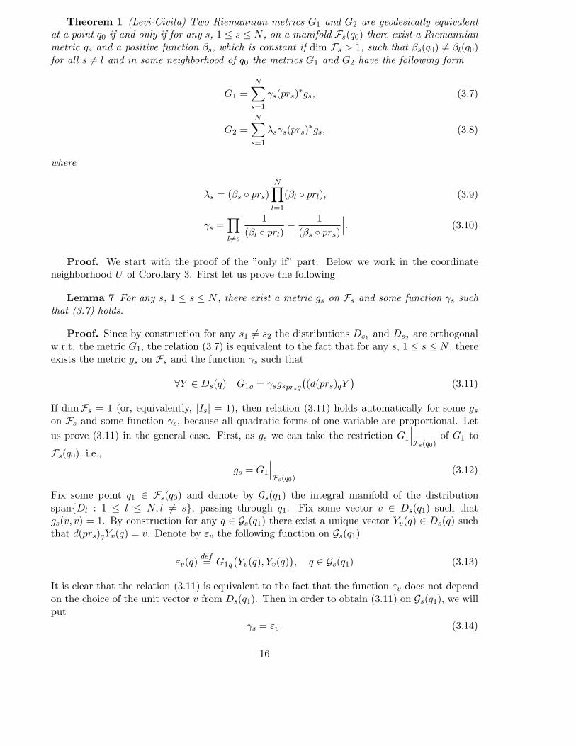
Theorem 1 (Levi-Civita) Two Riemannian metrics G1 and G2 are geodesically equivalentat a point q0 if and only if for any s, 1 ≤ s ≤ N , on a manifold Fs(q0) there exist a Riemannianmetric gs and a positive function βs, which is constant if dim Fs > 1, such that βs(q0) 6= βl(q0)for all s 6= l and in some neighborhood of q0 the metrics G1 and G2 have the following form

G1 =N∑

s=1

γs(prs)∗gs, (3.7)

G2 =

N∑

s=1

λsγs(prs)∗gs, (3.8)

where

λs = (βs prs)N∏

l=1

(βl prl), (3.9)

γs =∏

l 6=s

∣

∣

∣

1

(βl prl)− 1

(βs prs)∣

∣

∣. (3.10)

Proof. We start with the proof of the ”only if” part. Below we work in the coordinateneighborhood U of Corollary 3. First let us prove the following

Lemma 7 For any s, 1 ≤ s ≤ N , there exist a metric gs on Fs and some function γs suchthat (3.7) holds.

Proof. Since by construction for any s1 6= s2 the distributions Ds1and Ds2

are orthogonalw.r.t. the metric G1, the relation (3.7) is equivalent to the fact that for any s, 1 ≤ s ≤ N , thereexists the metric gs on Fs and the function γs such that

∀Y ∈ Ds(q) G1q = γsgsprsq

(

(d(prs)qY)

(3.11)

If dimFs = 1 (or, equivalently, |Is| = 1), then relation (3.11) holds automatically for some gs

on Fs and some function γs, because all quadratic forms of one variable are proportional. Let

us prove (3.11) in the general case. First, as gs we can take the restriction G1

∣

∣

∣

Fs(q0)of G1 to

Fs(q0), i.e.,

gs = G1

∣

∣

∣

Fs(q0)(3.12)

Fix some point q1 ∈ Fs(q0) and denote by Gs(q1) the integral manifold of the distributionspanDl : 1 ≤ l ≤ N, l 6= s, passing through q1. Fix some vector v ∈ Ds(q1) such thatgs(v, v) = 1. By construction for any q ∈ Gs(q1) there exist a unique vector Yv(q) ∈ Ds(q) suchthat d(prs)qYv(q) = v. Denote by εv the following function on Gs(q1)

εv(q)def= G1q

(

Yv(q), Yv(q))

, q ∈ Gs(q1) (3.13)

It is clear that the relation (3.11) is equivalent to the fact that the function εv does not dependon the choice of the unit vector v from Ds(q1). Then in order to obtain (3.11) on Gs(q1), we willput

γs = εv. (3.14)

16

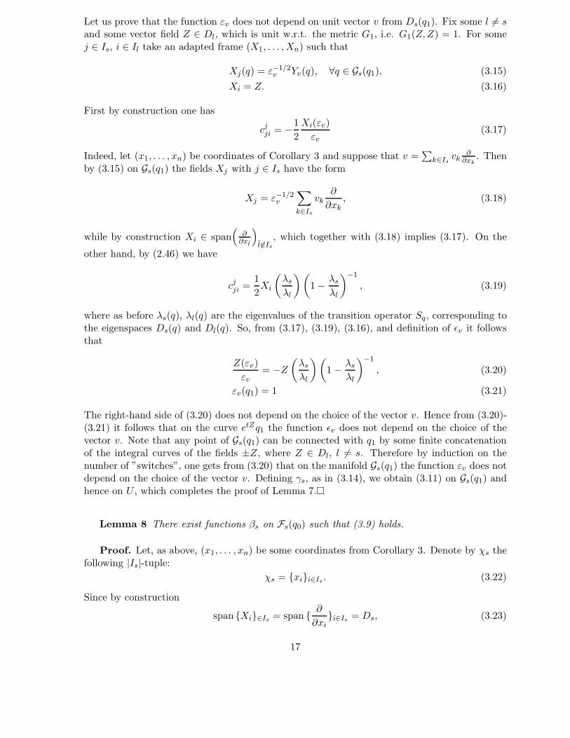
Let us prove that the function εv does not depend on unit vector v from Ds(q1). Fix some l 6= sand some vector field Z ∈ Dl, which is unit w.r.t. the metric G1, i.e. G1(Z,Z) = 1. For somej ∈ Is, i ∈ Il take an adapted frame (X1, . . . ,Xn) such that

Xj(q) = ε−1/2v Yv(q), ∀q ∈ Gs(q1), (3.15)

Xi = Z. (3.16)

First by construction one has

cjji = −1

2

Xi(εv)

εv(3.17)

Indeed, let (x1, . . . , xn) be coordinates of Corollary 3 and suppose that v =∑

k∈Isvk

∂∂xk

. Thenby (3.15) on Gs(q1) the fields Xj with j ∈ Is have the form

Xj = ε−1/2v

∑

k∈Is

vk∂

∂xk, (3.18)

while by construction Xi ∈ span(

∂∂xl

)

l 6∈Is

, which together with (3.18) implies (3.17). On the

other hand, by (2.46) we have

cjji =1

2Xi

(

λs

λl

)(

1 − λs

λl

)−1

, (3.19)

where as before λs(q), λl(q) are the eigenvalues of the transition operator Sq, corresponding tothe eigenspaces Ds(q) and Dl(q). So, from (3.17), (3.19), (3.16), and definition of ǫv it followsthat

Z(εv)

εv= −Z

(

λs

λl

)(

1 − λs

λl

)−1

, (3.20)

εv(q1) = 1 (3.21)

The right-hand side of (3.20) does not depend on the choice of the vector v. Hence from (3.20)-(3.21) it follows that on the curve etZq1 the function ǫv does not depend on the choice of thevector v. Note that any point of Gs(q1) can be connected with q1 by some finite concatenationof the integral curves of the fields ±Z, where Z ∈ Dl, l 6= s. Therefore by induction on thenumber of ”switches”, one gets from (3.20) that on the manifold Gs(q1) the function εv does notdepend on the choice of the vector v. Defining γs, as in (3.14), we obtain (3.11) on Gs(q1) andhence on U , which completes the proof of Lemma 7.

Lemma 8 There exist functions βs on Fs(q0) such that (3.9) holds.

Proof. Let, as above, (x1, . . . , xn) be some coordinates from Corollary 3. Denote by χs thefollowing |Is|-tuple:

χs = xii∈Is . (3.22)

Since by construction

span Xi∈Is = span ∂

∂xii∈Is = Ds, (3.23)

17

relations (2.47) and (2.48) are equivalent to the following relations respectively

∀1 ≤ s 6= l ≤ N, i ∈ Is :∂

∂xi

(

λ2l

λs

)

= 0, (3.24)

∀1 ≤ s, l, r ≤ N, l 6= s, r 6= s, i ∈ Is :∂

∂xi

(

λl

λr

)

= 0. (3.25)

First suppose that N = 2. Then from (3.24) there exist functions βs(χs), s = 1, 3 such that

λ22

λ1= β2(χ2),

λ21

λ2= β1(χ1), (3.26)

which easily implies (3.9), if we take β1 = β1/31 , β2 = β

1/32 . For N > 2 a standard analysis of

conditions (3.25) implies that there exist functions βs(χs) such that

λs(q)

λl(q)=βs(χs)

βl(χl)(3.27)

Substituting the last relation in (2.47) one can obtain easily that

∂

∂xj

(

λs(q)

βl(χl)

)

= 0, j ∈ Il, l 6= s (3.28)

Using standard arguments of ”separation of variables” for the last equations, one can easilyconclude that there exist a function σ(χs) such that

λs = σ(χs)∏

l 6=s

βl(χl). (3.29)

Substituting the last equation to (3.27) we obtain that

σs(χs)

σl(χl)=β2

s (χs)

β2l (χl)

,

which in turn implies that σi = Cβ2i for some constant C > 0. Replacing functions βi by kβi

for some constant k > 0 one can make C = 1. So,

λs = βs(χs)

N∏

l=1

βl(χl), (3.30)

which is equivalent to (3.9).

Lemma 9 If dimFs > 1, then λs is constant on each leaf of the foliation Fs

Proof. Taking the coefficients of u2i , i 6= j , from (2.60) and using (3.1), we obtain the

following relationXj(α

2i ) = 2ciji(α

2j − α2

i ) i 6= j. (3.31)

Note that identity (3.31) is stronger than identity (2.58): in the first identity we assume that thecorresponding indices are different, while in the second one we assume that the correspondingeigenvalues are different. Take any pair of indices i, j ∈ Is such that i 6= j (by assumption |Is| > 1

it is possible). Applying (3.31) and using the fact that αi = αj = λ1/2s , we get Xj(λs) = 0 for

any j ∈ Is, which implies the statement of the lemma.

18

Remark 3 The functions βs from relation (3.9) have the intrinsic meaning, because theycan be expressed by the eigenvalues of the transition operator Sq in the following way

βs prs = λN−1N+1

s

(

∏

l 6=s

λl

)− 2

N+1

(3.32)

From the previous lemma and (3.9) it follows immediately the following

Corollary 4 If dimFs > 1, then the function βs is constant.

To complete the ”only if” part it remains to prove relation (3.10). For this, combining (3.14),(3.17), and (3.19), then taking into account (3.23) and (3.27), one obtains without difficulties

∀1 ≤ s 6= l ≤ N, i ∈ Il :∂

∂xiln γs =

∂

∂xiln

∣

∣

∣

∣

βs(χs)

βl(χl)− 1

∣

∣

∣

∣

. (3.33)

Again using standard ”separation of variables” arguments we get from the last relations thatthere exist one-valuable functions ωs(χs) such that

γs = ωs(χs)∏

l 6=s

∣

∣

∣

∣

1

βl(χl)− 1

βs(χs)

∣

∣

∣

∣

. (3.34)

Finally note that by a change of coordinates of the type χs 7→ Fs(χs) we can make ωs ≡ 1 forany 1 ≤ s ≤ N , which together with (3.34) implies (3.10). This completes the proof of the ”onlyif” part.

Note that in the proof of the ”only if” part we actually have used all information, which canbe obtained from relations (3.1) (the only group of coefficients in (2.60) that we did not exploitare coefficients of uiuj with i 6= j, but the identities that they produce from (3.1) are equivalentto identities (3.31), which was obtained by exploiting another group of coefficients). Thereforeby Lemma 4 the conditions of the theorem are not only necessary, but also sufficient. The proofof the theorem is completed.

For metrics on surfaces Levi-Civita’s theorem is called also Dini’s Theorem, because Diniobtained it first in [2].

4 The case of corank one distributions

In the present section we investigate the problem of geodesic equivalence of sub-Riemannianmetrics on a distribution D of corank 1, especially, if D is contact or quasi-contact. From thebeginning we work in the neighborhood of regular point q0, extending then the results to thenon-regular points by the limiting process, when it is possible.

Let the functions Rj and Qjk be as in (2.18) and (2.19) respectively. All these functions arepolynomials on the fibers. In general, these functions depend on the choice of the adapted frameto the pair of the metrics (G1, G2).

Definition 6 We will say that the ordered pair (G1, G2) of sub-Riemannian metrics on thedistribution D satisfies the second divisibility condition on an open set U , if there exist an adaptedframe to the pair (G1, G2) in U such that for any q ∈ U on the fiber T ∗

q U the polynomial Rj isdivided by the polynomial Qjm+1 for any index j such that Qjm+1 6≡ 0 on T ∗

q U , 1 ≤ j ≤ m.

19

Note that cm+1ji = 1

αiαjcm+1ji for any i, j such that 1 ≤ i ≤ j. Therefore

Qjm+1 =1

αj

m∑

i=1

cm+1ji ui. (4.1)

Proposition 8 Suppose that for given two sub-Riemannian metrics G1 and G2 on corank 1distribution D and for some open set U of regular point q0 there exists an orbital diffeomorphismof the extremal flows of these metrics in some open set B in H1 ∩ T ∗U , π(B) = U . Then thepair (G1, G2) satisfies the second divisibility condition on U .

Proof. Fix some index j, 1 ≤ j ≤ m, such that

Qjm+1 6≡ 0. (4.2)

Substituting (2.37) into (2.21) we obtain

−~h1(Qjm+1)Rj

αjQ2jm+1P1/2

=polynomial

Qjm+1P3/2

or, equivalently,

P~h1(Qjm+1)Rj

Qjm+1= polynomial. (4.3)

Positive definite quadratic form P cannot be divided by Qjm+1, which is linear function with

real coefficients. Let us prove that Qjm+1 does not divide ~h1(Qjm+1). Assuming the converse,

one can conclude that the coefficients of ujum+1 in the quadratic polynomial ~h1(Qjm+1) has tobe equal to zero (because Qjm+1 does not depend both on uj and on um+1). On the other hand,from (2.24) and (4.1) it is not hard to get that this coefficient is equal to

− 1

αj

m∑

i=1

(

cm+1ji

)2.

Hence cm+1ji = 0 for all 1 ≤ i ≤ m, which contradicts the assumption (4.2). So, relation (4.3)

yields that Rj has to be divided by Qjm+1, i.e., the second divisibility condition holds.

Proposition 9 Suppose that for given two sub-Riemannian metrics G1 and G2 on some(m,m+ 1)-distribution D and for some open set U there exists an orbital diffeomorphism of theextremal flows of these metrics in some open set B in H1 ∩ T ∗U , π(B) = U . Suppose also thatthere exists the basis (X1, . . . ,Xm) of D adapted to the ordered pair (G1, G2), and the transitionoperator Sq has the form Sq = diag (α2

1(q), . . . , α2m(q)) in this basis (αi > 0). Then the following

two statements hold

1. If

Idef=

j ∈ 1, . . . ,m : [Xj ,D](q) 6⊂ D(q) ∀q ∈ U

, (4.4)

then αi = αj in U for all i, j ∈ I;

2. If αdef= αj , j ∈ I, and I =

j ∈ 1, . . . ,m : αj = α

, then

∀j ∈ I : Xj(α) = 0 (4.5)

20

Proof. By Proposition 8 for any j ∈ I the polynomial Rj is divided by αjQjm+1. But by

(2.37) the polynomialRj

αjQjm+1does not depend on j ∈ I (because it is equal to

√PΦm+1). In

other word,

Rj =(

m+1∑

i=1

riui

)

αjQjm+1, (4.6)

where coefficients ri do not depend on j ∈ I. As a consequence of the last identity and (2.37)one has

Φm+1 =

∑m+1i=1 riui√

P. (4.7)

Using (2.60) and (4.1), one can compare the coefficients of uium+1, 1 ≤ i ≤ m in both sides of(4.6) to get

α2jc

m+1ji = rm+1c

m+1ji .

Since by definition for any j ∈ I there exist 1 ≤ i ≤ m such that cm+1ji 6= 0, then

∀j ∈ I : α2j = rm+1 (4.8)

In other words, αj does not depend on j ∈ I, which concludes the proof of the first statementof the proposition.

Let us prove the second statement. From (2.60) and the fact that αj = αi = α for all i ∈ Iit follows that

∀i ∈ I :(

the coefficient of u2i in Rj

)

= −1

2Xj(α

2). (4.9)

If j ∈ I\I, then Qjm+1 = 0 and by identity (2.20) we have Rj = 0, which together with (4.9)implies that Xj(α

2) = 0.If j ∈ I, then comparing the coefficients of u2

i , i ∈ I, i 6= j in both sides of (4.6) and usingrelations (4.9), (4.1), we obtain

1

2Xj(α

2) = ricm+1ij . (4.10)

Substituting identity (4.7) into identity (2.21) with s = m + 1, then using (2.53), and finallymultiplying both sides on

√P, we get

~h1

(

m+1∑

i=1

riui

)

− 1

2

(

m∑

j=1

Xj(α2j )

α2j

uj

)

m+1∑

i=1

riui −Qm+1 m+1

m+1∑

i=1

riui =

m∑

k=1

Qm+1 kαkuk (4.11)

Comparing the coefficients of ujum+1, j ∈ I in both sides of (4.11) one can obtain withoutdifficulties that

m∑

i=1

ricm+1ij +

1

2Xj(α

2) = 0,

which together with (4.10) implies thatnj+1

2 Xj(α2) = 0, where nj is the number of indices i,

1 ≤ i ≤ m such that cm+1ij 6= 0. Therefore Xj(α

2) = 0 for all j ∈ I. The proof of the secondstatement is also completed.

As a direct consequence of Proposition 3 and the previous proposition we obtain the following

Theorem 2 If two sub-Riemannian metrics G1 and G2, defined on a contact distributionD, are geodesically equivalent at some point q0, then they are constantly proportional in someneighborhood of q0.

21

Proof. First note that it is sufficient to prove this theorem for regular q0: using the densityof the set of regular points (Proposition 1), one can extend the theorem to the non-regularpoints by passing to the limit. If q0 is regular, then there exists the basis (X1, . . . ,Xm) of Dadapted to the ordered pair (G1, G2). Let, as before, the transition operator Sq has the formSq = diag (α2

1(q), . . . , α2m(q)) in this basis (αi > 0). In the case of the contact distribution the

set I, defined by (4.4), coincides with 1, . . . ,m. Therefore, by consecutive use of Propositions3 and 9 we obtain that there exists the function α such that αi = α and Xi(α) = 0 for any i,1 ≤ i ≤ m. This together with the fact that contact distribution is bracket generating impliesthat αi = α = const for any i, 1 ≤ i ≤ m, which concludes the proof of the theorem.

For (2, 3)-distributions we can extend the last result from contact to all bracket-generatingdistributions, because the set of points, where bracket-generating (2, 3)- distributions are contact,is open and dense. Namely, we have the following

Corollary 5 If two sub-Riemannian metrics G1 and G2, defined on a bracket-generating(2, 3)-distribution D, are geodesically equivalent at some point q0, then they are constantly pro-portional in some neighborhood of q0.

Now consider the case of the quasi-contact distribution D. The following theorem gives theclassification of all geodesically equivalent sub-Riemannian metrics, defined on such distribution:

Theorem 3 Suppose that G1 and G2 are two sub-Riemannian metrics on the quasi-contactdistribution D such that G2 6≡ constG1. Assume also that the vector field X is tangent to theabnormal line distribution of D and unit w.r.t. the metric G1 (i.e., G1q(X,X) = 1). Then themetrics G1 and G2 are geodesically equivalent at the point q0 if and only if in some neighborhoodU of q0 the following four conditions hold simultaneously:

1. IfDi(q) = v ∈ D(q) : Giq(v,X) = 0, i = 1, 2, (4.12)

then D1(q) = D2(q) and the distribution D21 is codimension 1 integrable distribution (here

D21 = D1 + [D1,D1]);

2. If F is the foliation of the integral hypersurfaces of the distribution D21, then the flow etX

generated by the vector field X preserves the foliation F , i.e., it maps any leaf of F to aleaf of F ;

3. There exists the one-variable function β(t), β(0) = 1, such that if F0 is the leaf of the

foliation F passing through q0 and G1

∣

∣

∣

etxF0

is the restriction of the metric G1 to the leaf

etXF0, then

G1

∣

∣

∣

etXF0

= β(t)(

(e−tX )∗G1

)∣

∣

∣

etXF0

; (4.13)

4. There exist two constants C1 > 0 and C2 > −1, C2 6= 0, such that if F0 is as before and

G2

∣

∣

∣

etxF0

is the restriction of the metric G2 to the leaf etXF0, then

G2

∣

∣

∣

etXF0

=C1

1 + C2β(t)G1

∣

∣

∣

etXF0

, (4.14)

∀q ∈ etXF0 : G2q

(

X(q),X(q))

=C1

(

1 +C2β(t))2 . (4.15)

22

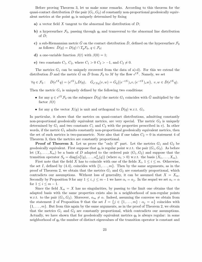
Before proving Theorem 3, let us make some remarks. According to this theorem for thequasi-contact distributionD the pair (G1, G2) of constantly non-proportional geodesically equiv-alent metrics at the point q0 is uniquely determined by fixing

a) a vector field X tangent to the abnormal line distribution of D;

b) a hypersurface F0, passing through q0 and transversal to the abnormal line distributionof D;

c) a sub-Riemannian metric G on the contact distribution D, defined on the hypersurface F0

as follows: D(q) = D(q) ∩ TqF0, q ∈ F0;

d) a one-variable function β(t) with β(0) = 1;

e) two constants C1, C2, where C1 > 0 C2 > −1, and C2 6= 0.

The metrics G1 can be uniquely recovered from the data of a)-d). For this we extend thedistribution D and the metric G on D from F0 to M by the flow etX . Namely, we set

∀q ∈ F0 : D(etXq) = (etX)∗D(q), GetXq(v,w) = Gq

(

(e−tX )∗v, (e−tX )∗w

)

, v, w ∈ D(etXq).

Then the metric G1 is uniquely defined by the following two conditions:

• for any q ∈ etXF0 on the subspace D(q) the metric G1 coincides with G multiplied by thefactor β(t)

• for any q the vector X(q) is unit and orthogonal to D(q) w.r.t. G1.

In particular, it shows that the metrics on quasi-contact distributions, admitting constantlynon-proportional geodesically equivalent metrics, are very special. The metric G2 is uniquelydetermined by G1 and two constants C1 and C2 with the properties prescribed in e). In otherwords, if the metric G1 admits constantly non-proportional geodesically equivalent metrics, thenthe set of such metrics is two-parametric. Note also that if one takes C2 = 0 in statement 4 ofTheorem 3, then the metrics are constantly proportional.

Proof of Theorem 3. Let us prove the ”only if” part. Let the metrics G1 and G2 begeodesically equivalent. First suppose that q0 is regular point w.r.t. the pair (G1, G2). As beforelet (X1, . . . ,Xm) be a basis of D adapted to the ordered pair (G1, G2) and suppose that thetransition operator Sq = diag

(

α21(q), . . . , α

2m(q)

)

(where αi > 0) w.r.t. the basis (X1, . . . ,Xm).First note that the field X has to coincide with one of the fields Xi, 1 ≤ i ≤ m. Otherwise,

the set I, defined by (4.4), coincides with 1, . . . ,m. Then by the same arguments, as in theproof of Theorem 2, we obtain that the metrics G1 and G2 are constantly proportional, whichcontradicts our assumptions. Without loss of generality, it can be assumed that X = Xm.Secondly by Proposition 9 for any 1 ≤ i, j ≤ m−1 we have αi = αj . In the sequel we set αi = αfor 1 ≤ i ≤ m− 1.

Since the field Xm = X has no singularities, by passing to the limit one obtains that theadapted basis with the same properties exists also in a neighborhood of non-regular pointsw.r.t. to the pair (G1, G2). Moreover, αm 6= α. Indeed, assuming the converse we obtain fromthe statement 2 of Proposition 9 that the set I =

j ∈ 1, . . . ,m : αj = α

coincides with1, . . . ,m. But from this again by the same arguments, as in the proof of Theorem 2, we obtainthat the metrics G1 and G2 are constantly proportional, which contradicts our assumptions.Actually, we have shown that for geodesically equivalent metrics q0 is always regular: in someneighborhood of q0 the number of distinct eigenvalues of the transition operator is constant and

23

equal either to 1 (in this case the metrics are constantly proportional) or to 2. Besides, if D1

and D2 are as in (4.12), then

D1 = D2 = span(X1, . . . ,Xm−1).

From (2.47) it follows that Xi

(

α2m

α

)

= 0 for all 1 ≤ i ≤ m − 1, which together with (4.5)

implies∀1 ≤ i ≤ m− 1 : Xi(αm) = 0. (4.16)

Replacing the (4.5) and (4.16) in (2.46), we obtain also that

∀1 ≤ i ≤ m− 1 : cmmi = 0. (4.17)

Let us complete the adapted basis (X1, . . . ,Xm) somehow to the frame (X1, . . . ,Xm+1).

Lemma 10 The distribution D21 = D1 + [D1,D1] is integrable.

Proof. Using (2.60) and (4.1), let us compare the coefficients of uium, 1 ≤ i ≤ m− 1 in bothsides of (4.6), where 1 ≤ j ≤ m− 1. As a result, we get easily

∀1 ≤ i 6= j ≤ m− 1 : (α2 − α2m)cmji = rmc

m+1ji + ric

m+1jm .

But by construction m 6∈ I, i.e., cm+1jm = 0 for all 1 ≤ j ≤ m − 1. Therefore the last relation is

equivalent to the following identity:

∀1 ≤ i 6= j ≤ m− 1 : cmji =rm

α2 − α2m

cm+1ji . (4.18)

Hence [Xi,Xj ] ∈ span(

X1, . . . ,Xm−1,rm

α2−α2mXm +Xm+1

)

for all 1 ≤ i, j ≤ m − 1 or , equiva-

lently,

D21 = span

(

D1,rm

α2 − α2m

Xm +Xm+1

)

. (4.19)

To prove the lemma it is sufficient to prove that

∀1 ≤ i ≤ m− 1 :[

Xi,rm

α2 − α2m

Xm +Xm+1

]

∈ span(

D1,rm

α2 − α2m

Xm +Xm+1

)

. (4.20)

Using (4.5) and (4.16), it is easy to show that (4.20) is equivalent to the following identity

Xi(rm) + rmcmmi + cmm+1i(α

2 − α2m) − rmc

m+1m+1 i = 0 (4.21)

Let us prove identity (4.21). First note that from (4.5) and (4.10) it follows easily that ri = 0for 1 ≤ i ≤ m − 1 (here we use also the fact that for given i, 1 ≤ i ≤ m − 1, there exist j,1 ≤ j ≤ m− 1, such that cm+1

ij 6= 0). From this and (4.5) it follows that the identity (4.11) canbe rewritten in the following form:

~h1

(

m+1∑

i=m

riui

)

− 1

2

Xm(α2m)

α2m

um

m+1∑

i=m

riui −Qm+1 m+1

m+1∑

i=m

riui =

m∑

k=1

Qm+1 kαkuk (4.22)

Comparing the coefficients of uium, 1 ≤ i ≤ m − 1 in both sides of (4.22) by use of (2.24) and(2.19) it is not difficult to obtain

Xi(rm) + rmcmmi + rm+1(c

mm+1i + cim+1m) − rmc

m+1m+1 iα = (cim+1m + cmm+1i)ααm (4.23)

From (2.61) and (2.22) it follows that cm+1m+1 i = 1

αcm+1m+1 i, c

im+1m = α

αmcim+1m, and cmm+1i =

αm

α cmm+1i, while by (4.8) we have rm+1 = α2. Substituting all this to (4.23) we get (4.21), whichcompletes the proof of the lemma.

24

Lemma 11 If F is the foliation of the integral hypersurfaces of the distribution D21, then

the flow etX generated by the vector field X preserves the foliation F .

Proof. From the previous lemma it follows that in some neighborhood U of q0 there ex-ist coordinates (x1, . . . , xm+1) such that the leaves of F are xm = const and Xm = ν ∂

∂xm

for some function ν. By construction, all vector fields Xi with 1 ≤ i ≤ m − 1 belong tospan

(

∂∂x1

, . . . , ∂∂xm−1

, ∂∂xm+1

)

. Therefore cmmi = Xi(ν)ν for all 1 ≤ i ≤ m− 1, which together with

(4.17) implies that Xi(ν) = 0 for all 1 ≤ i ≤ m− 1. Then ν is constant on each leaf of F , whichequivalent to the statement of the lemma.

Lemma 12 Relation (4.13) holds for some one-variable function β(t).

Proof. Actually the proof of this lemma is very similar to the proof of Lemma 7. Since thevector field X = Xm satisfies [X,D] ⊂ D, the flow etX preserves the distribution D. This andthe previous lemma implies that etX preserves also the distributionD1 (note that by the previouslemma D1(q) = D(q) ∩ TqF(q), where F(q) is the leaf of the foliation F , passing through thepoint q).

Fix some point q1 ∈ F0. Denote by Lq1the abnormal extremal trajectory passing through

q1. Fix some vector v ∈ Ds(q1) such that G1q1(v, v) = 1. By construction for any point q ∈ Lq1

such that q = etXq1 there exist a unique vector Yv(q) ∈ D1(q) such that d(e−tX )qYv(q) = v.Denote by εv the following function on the curve Lq1

.

εv(q)def= G1q

(

Yv(q), Yv(q))

, q ∈ Lq1(4.24)

By the same arguments as in the proof of Lemma 7, we obtain that the function εv does notdepend on the choice of the unit vector v from D1(q1). It implies that for any q in someneighborhood U of q0 (here any coordinate neighborhood from the proof of the previous lemmacan be taken as U) there is β(q) such that if q = etXq1, where q1 ∈ F0, then

G1

∣

∣

∣

etXF0

= β(

(e−tX )∗G1

)∣

∣

∣

etXF0

(4.25)

Besides, similarly to (3.20)-(3.21), we have

X(β)

β= −X

(

α2

α2m

)(

1 − α2

α2m

)−1

, (4.26)

β∣

∣

∣

F0

= 1. (4.27)

Finally by (4.5) and (4.16) the functions α and αm are constant on each leaf of the foliationF . Therefore (4.26)-(4.27) implies that the function β is constant on each leaf of the foliationF too. This fact together with (4.25) implies (4.13).

In order to complete the proof of the ”only if” part it remains to prove identities (4.14) and(4.15). By (2.12) and statement 1 of Proposition 9

∀q ∈ etXF0 : G2q = α2(q)G1q (4.28)

∀q ∈ etXF0 : G2q

(

X(q),X(q))

= α2m(q). (4.29)

25

So, it remains to find the functions α and αm. As was mentioned in the proof of the previouslemma, the functions α and αm are constant on each leaf of the foliation F . Besides, by (2.47)

we have Xm( α2

αm) = 0. So,

α2

αm≡ C, (4.30)

where C is constant. Then from (2.46) it follows that for any j, 1 ≤ j ≤ m− 1

Xm

(

C

αm

)

= 2cjjm

(

1 − C

αm

)

(4.31)

By Lemmas 10-12 we can choose the coordinates (y1, . . . , ym, t) in a neighborhood of q0 suchthat q0 = (0, . . . , 0) and

Xm =∂

∂t; (4.32)

Xj = β(t)−1/2m∑

k=1

νjk∂

∂yk, 1 ≤ j ≤ m− 1. (4.33)

As in (3.17) this yields that

cjjm = −1

2

d

dtlnβ(t).

Substituting the last formula in (4.31), one can obtain without difficulties that

αm =C

1 + C2β(t)(4.34)

for some constant C2, C2 > −1, C2 6= 0. Then by (4.30)

α2 = Cαm =C2

1 + C2β(t)(4.35)

Setting C1 = C2 and substituting (4.35) and (4.34) into (4.28) and (4.29), we get (4.14) and(4.15). The proof of the ”only if” part of the theorem is completed.

Note that in the proof of the ”only if ” part we actually have used all information, containedin (4.6), which is equivalent to (2.20). Also, it can be shown by direct check that if all conditions1-4 of Theorem 3 hold then the identity (4.22) holds too (but this identity is equivalent to (2.21)).From this, Lemma 2, and Proposition 2 it follows that conditions 1-4 of the theorem are alsosufficient for the geodesic equivalence of our metrics at q0.

5 The case of Riemannian metrics on a surface near non-regular

isolated point

In the present section for the Riemannian metrics on a surface we obtain the classificationof geodesically equivalent pairs at non-regular point (the point of bifurcation of the eigenvaluesof the transition operator). Namely, we consider the case when two Riemannian metrics on asurface are proportional in an isolated point. Since the set of all 2× 2 symmetric matrices withthe equal eigenvalues has codimension 2 in the set of all 2× 2 symmetric matrices, we have thatfor generic pair of Riemannian metrics on a surface the set of points of their proportionalityconsists of isolated points. Therefore its is natural to consider the case when two Riemannian

26

metrics on a surface are proportional in an isolated point. It turns out that Dini’s Theorem(i.e., Levi-Civita’s theorem in the case of a surface) can be naturally extended to this case.

First let us formulate Dini’s Theorem in the case of non-proportional metrics and analyzeits additional features.

Theorem 4 (Dini’s Theorem) Suppose that two Riemannian metrics G1 and G2 on a sur-face are non-proportional at some point q0. Then they are geodesically equivalent at q0 if and onlyif in some neighborhood of q0, there exist coordinates (x1, x2), q0 = (x0

1, x02), and one-variable

functions β1(x1) and β2(x2) (β1(x01) < β2(x

02)) such that in this coordinates

|| · ||21 =

(

1

β1(x1)− 1

β2(x2)

)

(dx21 + dx2

2), (5.1)

|| · ||22 = β1(x1)β2(x2)

(

1

β1(x1)− 1

β2(x2)

)

(

β1(x1)dx21 + β2(x2)dx

22

)

, (5.2)

where ||v||2i = Gi(v, v), i = 1, 2.

The coordinates, appearing in Theorem 4, will be called Dini’s coordinates of the orderedpair of Riemannian metrics (G1, G2). The following lemma will be useful in the sequel

Lemma 13 If (x1, x2) and (x1, x2) are two Dini’s coordinates of the ordered pair of Rie-mannian metrics (G1, G2) on the same neighborhood U , then xi = ±xi + ci some constants ci,i = 1, 2.

Proof. From Corollary 3 and the fact that in Theorem 1 we assume that β1(x01) < β2(x

02)

it follows that the coordinate net of all Dini’s coordinates on U coincide: D1 = dx2 = 0 =dx2 = 0 is the line distribution of the eigenvectors of the transition operator, correspondingto its smallest eigenvalue, while D2 = dx1 = 0 = dx1 = 0 is the line distribution ofthe eigenvectors of the transition operator, corresponding to its biggest eigenvalue. Hence thetransition function between the coordinates has a form xi = ψi(xi), i = 1, . . . n. Then the firstmetric is written in the coordinates (x1, . . . , xn) as follows:

|| · ||21 =

(

1

β1

(

ψ(x1)) − 1

β22

(

ψ(x2))

)

2∑

j=1

(ψ′i(xj))

2(d xj)2.

By Remark 3 the coefficients of dx2j in (5.1) do not depend on the choice of the Dini coordinates.

Therefore (ψ′i(xj))

2 ≡ 1, which implies the statement of the Lemma.

Recall that a Riemannian metric on a surface defines the canonical conformal structure: Ina neighborhood of any point there is a coordinate system in which the Riemannian metric hasthe form

|| · ||2 = µ(x, y)(dx2 + d y2). (5.3)

Such coordinates are called isothermal (see, for example, [8] or [3]). The transition functionfrom one isothermal coordinates to some other is conformal mapping, up to the orientation, sothe set of all charts with isothermal coordinates defines the conformal structure. Note that by(5.1) all Dini’s coordinates are isothermal w.r.t. the first metric G1.

Now suppose that the Riemannian metrics G1 and G2 are proportional at some isolatedpoint q0 and geodesic equivalent in a neighborhood of this point. Choose in a neighborhood Bof q0 some isothermal coordinates (x, y) w.r.t. the first metric G1. Also, we can assume that the

27

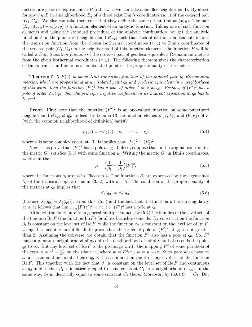
metrics are geodesic equivalent in B (otherwise we can take a smaller neighborhood). By abovefor any q ∈ B in a neighborhood Bq of q there exist Dini’s coordinates (u, v) of the ordered pair(G1, G2). We also can take them such that they define the same orientation as (x, y). The pair(Bq, u(x, y) + iv(x, y) is a function element of an analytic function. Taking one of such functionelements and using the standard procedure of the analytic continuation, we get the analyticfunction F in the punctured neighborhood B\q0 such that each of its function elements definesthe transition function from the chosen isothermal coordinates (x, y) to Dini’s coordinates ofthe ordered pair (G1, G2) in the neighborhood of this function element. The function F will becalled a Dini transition function of the ordered pair of geodesic equivalent Riemannian metricsfrom the given isothermal coordinates (x, y). The following theorem gives the characterizationof Dini’s transition functions at an isolated point of the proportionality of the metrics:

Theorem 5 If F (z) is some Dini transition function of the ordered pair of Riemannianmetrics, which are proportional at an isolated point q0 and geodesic equivalent in a neighborhoodof this point, then the function (F ′)2 has a pole of order 1 or 2 at q0. Besides, if (F ′)2 has apole of order 2 at q0, then the principle negative coefficient in its Laurent expansion at q0 has tobe real.

Proof. First note that the function (F ′)2 is an one-valued function on some puncturedneighborhood B\q0 of q0. Indeed, by Lemma 13 the function elements (V, F1) and (V, F2) of F(with the common neighborhood of definition) satisfy

F1(z) ≡ ±F2(z) + c, z = x+ iy, (5.4)

where c is some complex constant. This implies that (F ′1)

2 ≡ (F ′2)

2.

Now let us prove that (F ′)2 has a pole at q0. Indeed, suppose that in the original coordinatesthe metric G1 satisfies (5.3) with some function µ. Writing the metric G1 in Dini’s coordinates,we obtain that

µ =( 1

β1− 1

β2

)

|F ′|2, (5.5)

where the functions βi are as in Theorem 4. The functions βi are expressed by the eigenvaluesλj of the transition operator as in (3.32) with n = 2. The condition of the proportionality ofthe metrics at q0 implies that

β1(q0) = β2(q0) (5.6)

(because λ1(q0) = λ2(q0)). From this, (5.5) and the fact that the function µ has no singularityat q0 it follows that limz→q0

|F ′(z)|2 = ∞, i.e. (F ′)2 has a pole at q0.

Although the function F is in general multiple-valued, by (5.4) the families of the level sets ofthe function ReF (the function ImF ) for all its branches coincide. By construction the functionβ1 is constant on the level set of ReF , while the function β2 is constant on the level set of ImF .Using this fact it is not difficult to prove that the order of pole of (F ′)2 at q0 is not greaterthan 2. Assuming the converse, we obtain that the function F 2 also has a pole at q0. So, F 2

maps a puncture neighborhood of q0 onto the neighborhood of infinity and also sends the pointq0 to ∞. But any level set of ReF is the preimage w.r.t. the mapping F 2 of some parabola ofthe type u = c2 − v2

4c2 on the plane w, where w = F 2(z), w = u + iv. Such parabolas have ∞as an accumulation point. Hence q0 is the accumulation point of any level set of the functionReF . This together with the fact that β1 is constant on the level set of ReF and continuousat q0 implies that β1 is identically equal to some constant C1 in a neighborhood of q0. In thesame way, β2 is identically equal to some constant C2 there. Moreover, by (5.6) C1 = C2. But

28

it means that our metrics are proportional in the neighborhood of q0, which contradicts ourassumptions. So, the order of pole of (F ′)2 at q0 is not greater than 2.

To complete the proof of the theorem it remains to show that if (F ′)2 has a pole of order 2 atq0, then the principle negative coefficient in its Laurent expansion at q0 is real. Indeed, if (F ′)2

has a pole of order 2 with the principle negative coefficient a in its Laurent expansion at q0,then F has the logarithmic singularity at q0 with coefficient

√a near the logarithm. In this case

after the appropriate change of independent variable z in a neighborhood of q0 (i.e., conformalchange of coordinates in a neighborhood of q0) one can get F (z) =

√a log z, q0 = 0. But if a is

not real, then√a is neither real nor pure imaginary. In this case all level sets of both ReF and

ImF are spirals having q0, as an accumulation point. As above, it implies that functions β1 andβ2 are equal to the same constant, which is impossible. The proof of the theorem is completed.

According to the previous theorem only the following two situation are possible at an isolatedpoint of proportionality of two metrics:

1) (F ′)2 has a simple pole at q0 ⇔ F (z) =√

G(z) for some analytic function G(z), havingat q0 zero of order 1 (i.e., F has the ”square root” singularity at q0). In this case after theappropriate change of independent variable z in a neighborhood of q0 one can get F (z) =

√z,

q0 = 0;2) F ′ has a simple pole at q0 with real or pure imaginary residue at q0 ⇔ F (z) has the

logarithmic singularity at q0 with real or pure imaginary coefficient b near logarithm. In thiscase after the appropriate change of independent variable z in a neighborhood of q0 one can getF (z) = b log z, q0 = 0, where b is real or pure imaginary constant. If b is real then the levelsets of ImF (z) are the rays, starting at 0. Hence by the same argument as in the proof of theprevious theorem we can conclude that the function β2 is constant. Besides, the function β1 inthis case depends only on |z| (here βi as in Theorem 1). In the same way, if b is pure imaginary,then β1 is constant and β2 depends only on |z|.

Using 1), 2) and Theorem 1, we obtain without difficulties the following analog of Dini’sTheorem:

Theorem 6 (Generalization of Dini’s Theorem to the case of an isolated non-regular point)Two Riemannian metrics G1 and G2 on a surface M , which are proportional in an isolated pointq0, are geodesic equivalent in a neighborhood of this point if and only if one of the following twoconditions holds:

1. In a neighborhood of q0, there exist coordinates (x, y), q0 = (0, 0) and two one-variablesmooth functions U and V , satisfying 0 < U(u) < V (0) = U(0) < V (v) for all positive uand v, U ′(0) = −V ′(0), and V ′(0) > 0, such that in the punctured neighborhood of q0 themetrics G1 and G2 satisfy

|| · ||21 =

1

U(

r cos2 θ2

) − 1

V(

r sin2 θ2

)

1

4r(dr2 + r2dθ2), (5.7)

|| · ||22 =S

8r

(

(A− S cos θ)dr2 − 2Sr sin θdrdθ + (A+ S cos θ)r2dθ2)

, (5.8)

where

A = U(

r cos2θ

2

)

+ V(

r sin2 θ

2

)

, S = V(

r sin2 θ

2

)

− U(

r cos2 θ

2

)

,

and (r, θ) are the corresponding polar coordinates;

29

2. In a neighborhood of q0, there exist coordinates (x, y), q0 = (0, 0), positive constants a, C,and an one-variable smooth functions R(r), satisfying R(r) 6= R(0) for r > 0, R(0) = C,R′(0) = 0, and R′′(0) 6= 0, such that in the punctured neighborhood of q0 the metrics G1

and G2 satisfy

|| · ||21 =

∣

∣

∣

∣

1

C− 1

R(r)

∣

∣

∣

∣

a

r2(dr2 + r2dθ2), (5.9)

|| · ||22 =aCR(r)

r2

∣

∣

∣

∣

1

C− 1

R(r)

∣

∣

∣

∣

(

R(r)dr2 + Cr2dθ2)

, (5.10)

where (r, θ) are the corresponding polar coordinates.

Remark 4 The conditions on the functions U and V in the case 1 and on R in the case 2follows easily from the fact that the metrics are positive definite and nonsingular at q0.

Remark 5 Using the standard arguments of Complex Analysis, one can show that for thepair of geodesically equivalent metrics the set of non-regular points cannot be a rectifiable curveΓ: in this case one can construct an one-valued Dini transition conformal function out of Γwhich goes to infinity, when one tends to Γ. Then by Morera Theorem the function 1/F isanalytic and equal to zero on Γ and so everywhere, which is impossible.

Acknowledgments. I would like to thank professor A. Agrachev for proposing me to work onthis problem and for his constant attention to this work.

References

[1] E. Beltrami, Teoria fondamentale degli spazii di curvatura costante, Annali di matem.,ser.3, vol. 2, 1869, pp 269-287.

[2] U. Dini, Sopra un problema che si presenta nella teoria generale delle rappresentazionegeografiche di una superficie su di un’ altra, Annali di matem., ser 2, vol 3, 1870, 269-287.

[3] L.P. Eisenhart, An Introduction to Differential Geometry, Princeton University Press, 1947,304 p.

[4] T. Levi-Civita, Sulle trasformazioni delle equazioni dinamiche, Ann. Mat. Ser. 2a,24(1896),255-300.

[5] W.S. Liu, H. J. Sussmann, Shortest paths for sub-Riemannian metrics of rank two distri-butions, Memoirs AMS 118, no. 564, 1995.

[6] V.S. Matveev, P.I. Topalov, Geodesic Equivalence of Metrics of Surfaces and Their Inte-grability, Doklady Mathematics, Vol. 60, No. 1, 1999, 112-114; translated from DokladyAkademii Nauk, Vol 367, No.6, 1999, 736-738.

[7] V.S Matveev, P. Topalov, Geodesic equivalence via Integrability, Geometriae Dedicata 96,2003, 91-115.

[8] G. Springer, Introduction to Riemann Surfaces, Chelsey Publishing Company, New York,1981, 309 pages.

30