ZERO-MOMENT POINT WALKING CONTROLLER FOR HUMANOID

WALKING USING DARWIN-OP

Abstract

by

Joseph Rudy

The design and implementation of gait generation for stable steady-state hu-

manoid walking is a complex problem due to the high dimensional control space as

well as the inherently unstable motion. Moreover, humanoids must have a fast walk-

ing gait that models a human gait. This thesis aims to implement a stable walking

controller using the computed Zero-Moment Point (ZMP) method with a simplified

mass model of a humanoid robot, namely a cart-table model. From this simpli-

fied model, a center of mass (CoM) trajectory can be obtained and tracked using

the stance foot to achieve the desired ZMP. A swing leg trajectory can be obtained

through walking parameters such as stride length, stride width, and ground clear-

ance. Using this controller, a more human-like gait can be achieved in a humanoid

for faster steady-state walking.

CONTENTS

FIGURES . . . . . . . . . . . . . . . . . . . . . . . . . . . . . . . . . . . . . . iv

TABLES . . . . . . . . . . . . . . . . . . . . . . . . . . . . . . . . . . . . . . v

SYMBOLS . . . . . . . . . . . . . . . . . . . . . . . . . . . . . . . . . . . . . vi

ACKNOWLEDGMENTS . . . . . . . . . . . . . . . . . . . . . . . . . . . . . viii

CHAPTER 1: INTRODUCTION . . . . . . . . . . . . . . . . . . . . . . . . . 11.1 ZMP FOR BIPEDAL ROBOTS . . . . . . . . . . . . . . . . . . . . . 21.2 COMPUTED ZMP . . . . . . . . . . . . . . . . . . . . . . . . . . . . 31.3 THE HUMAN GAIT AND A SIMPLIFIED MODEL . . . . . . . . . 51.4 DARWIN-OP . . . . . . . . . . . . . . . . . . . . . . . . . . . . . . . 7

CHAPTER 2: METHODS . . . . . . . . . . . . . . . . . . . . . . . . . . . . . 102.1 CONTROLLER AND TRAJECTORY GENERATION SCHEME . . 10

2.1.1 DEFINING ANGLES . . . . . . . . . . . . . . . . . . . . . . 122.2 CENTER OF MASS TRAJECTORY . . . . . . . . . . . . . . . . . . 12

2.2.1 PREVIEW CONTROLLER . . . . . . . . . . . . . . . . . . . 162.3 SWING FOOT TRAJECTORY . . . . . . . . . . . . . . . . . . . . . 19

2.3.1 INITIAL SWING . . . . . . . . . . . . . . . . . . . . . . . . . 212.3.2 MIDSWING . . . . . . . . . . . . . . . . . . . . . . . . . . . . 232.3.3 TERMINAL SWING . . . . . . . . . . . . . . . . . . . . . . . 23

CHAPTER 3: IMPLEMENTATION . . . . . . . . . . . . . . . . . . . . . . . 263.1 REFERENCE GENERATION . . . . . . . . . . . . . . . . . . . . . 263.2 INVERSE KINEMATICS . . . . . . . . . . . . . . . . . . . . . . . . 29

3.2.1 STANCE LEG . . . . . . . . . . . . . . . . . . . . . . . . . . 293.2.1.1 PARALLEL BODY CONSTRAINT . . . . . . . . . 34

3.2.2 SWING LEG . . . . . . . . . . . . . . . . . . . . . . . . . . . 353.2.2.1 PARALLEL FOOT CONSTRAINT . . . . . . . . . 37

3.3 CONTROLLER ADDITIONS . . . . . . . . . . . . . . . . . . . . . . 383.4 PROGRAMMING SYNOPSIS . . . . . . . . . . . . . . . . . . . . . . 41

ii

CHAPTER 4: RESULTS AND DISCUSSION . . . . . . . . . . . . . . . . . . 454.1 TRIALS . . . . . . . . . . . . . . . . . . . . . . . . . . . . . . . . . . 454.2 DISCUSSION . . . . . . . . . . . . . . . . . . . . . . . . . . . . . . . 474.3 FUTURE WORK . . . . . . . . . . . . . . . . . . . . . . . . . . . . . 484.4 CONCLUSION . . . . . . . . . . . . . . . . . . . . . . . . . . . . . . 49

APPENDIX A: ZERO-MOMENT POINT . . . . . . . . . . . . . . . . . . . . 50A.1 TORQUE ABOUT ZMP . . . . . . . . . . . . . . . . . . . . . . . . . 50A.2 ZMP IN 3D DYNAMICS . . . . . . . . . . . . . . . . . . . . . . . . . 51A.3 3D LINEARIZED CART-TABLE MODEL . . . . . . . . . . . . . . . 53

APPENDIX B: OPTIMAL CONTROL DESIGN FOR A PREVIEW CON-TROLLER . . . . . . . . . . . . . . . . . . . . . . . . . . . . . . . . . . . 57

APPENDIX C: INVERSE KINEMATICS . . . . . . . . . . . . . . . . . . . . 60

BIBLIOGRAPHY . . . . . . . . . . . . . . . . . . . . . . . . . . . . . . . . . 64

iii

FIGURES

1.1 Definition of Zero-Moment Point [7] . . . . . . . . . . . . . . . . . . . 2

1.2 Cart-Table Model . . . . . . . . . . . . . . . . . . . . . . . . . . . . . 4

1.3 Human Gait Cycle [2] . . . . . . . . . . . . . . . . . . . . . . . . . . 5

1.4 DARwIn-OP with Coordinate Systems . . . . . . . . . . . . . . . . . 8

2.1 Control Scheme for the ZMP Walking Controller . . . . . . . . . . . . 11

2.2 3D Cart-Table Model . . . . . . . . . . . . . . . . . . . . . . . . . . . 13

2.3 Response of the Cart-Table Model Using No Preview Controller . . . 15

2.4 Block Diagram of Preview Controller . . . . . . . . . . . . . . . . . . 17

2.5 Preview Gains Using the Optimal Controller Design . . . . . . . . . . 19

2.6 Response of the Cart-Table Model Using the Preview Controller . . . 19

2.7 Humanoid Feet with the F Frame and N Frame . . . . . . . . . . . . 21

2.8 Possible Swing Foot Trajectory, pswing . . . . . . . . . . . . . . . . . 22

3.1 Vectors used to Identify the Location of the Foot and ZMP at Each Step 28

3.2 Local Coordinate Systems for DARwIn-OP . . . . . . . . . . . . . . . 30

3.3 Stance Leg Pitch Angles Forming the Height of the Pendulum . . . . 31

3.4 Graphs for the f , c, and cN/F as Functions of Time for a Possible Gait 32

3.5 Global Knee Angles without (left) and with (right) Knee Flexion Con-troller . . . . . . . . . . . . . . . . . . . . . . . . . . . . . . . . . . . 40

3.6 Flow Chart for the Implementation of the Controller . . . . . . . . . 42

3.7 Representation for the Queue of Steps in the Step Manager . . . . . . 43

A.1 Example of a Multi-Body System in 3 Dimensions . . . . . . . . . . . 51

A.2 3D Cart-Table Model . . . . . . . . . . . . . . . . . . . . . . . . . . . 54

iv

TABLES

2.1 Local and Global Angle Definitions . . . . . . . . . . . . . . . . . . . 12

4.1 Tests on Surface 1 . . . . . . . . . . . . . . . . . . . . . . . . . . . . . 464.2 Tests on Surface 2 . . . . . . . . . . . . . . . . . . . . . . . . . . . . . 46

v

SYMBOLS

α fraction of time spent in initial and terminal swing

b conversion constant from time to stride length

c center of mass

Cj i describes rotation from outer body, i, to inner body,j

cN/F center of mass relative to the F frame

cg ground clearance in [m]

d absolute value of difference between p and f

δ ZMP reference offset

∆p p5 swing − p5 hip

η ratio of stride width to stride length

f location of the F frame relative to the N frame

F local foot reference frame

fl foot length, 0.104 m

fw foot width, 0.066 m

f ref foot reference locating the location of previous swing foot

GI integral gain for cart-table controller

Gp preview gains for cart-table controller

Gx state feedback gains for cart-table controller

hp height of 3D pendulum in CoM tracking

Ip p× p identity matrix

vi

Kbp proportional gain for body pitch controller

Kkf proportional gain for knee flexion controller

N global inertial reference frame

ν CoM offset

p location of ZMP

phip location of swing hip relative to F frame

pref ZMP reference for the desired ZMP

pswing vector pointing from stance to swing foot

s foot path vector

sw stance width, 0.074 m

S stride vector

T step period

Ts sampling time, 8 ms

TDS period of double support

TSS period of single support

zc constant height of the cart off the ground in cart-table model

vii

ACKNOWLEDGMENTS

I would like to thank my advisor, Professor Jim Schmiedeler, for all his support

and guidance throughout my three years of research. I would like also to thank Pro-

fessors Bill Goodwine and Michael Stanisic for participating in my defense committee.

viii

CHAPTER 1

INTRODUCTION

The design and implementation of gait generation for stable steady-state humanoid

walking is a complex problem due to the high dimensional control space as well as

the inherently unstable motion. Moreover, humanoids must have a fast walking gait

and a gait that models the human gait. Many humanoid walking controllers use the

center of mass (CoM) to ensure static stability throughout the gait. Static stability

implies that the projection of the CoM onto the support surface is inside the support

polygon of the stance foot or feet throughout the gait. These CoM walking controllers

have a very long time period between steps, or a slow cadence, and do not model

human walking very well. However, a walking controller which can provide dynamic

stability allows for a faster cadence and a more human-like gait. Dynamic stability

implies that a point, called the Zero-Moment Point (ZMP), is inside the support

polygon throughout the gait.

In order to achieve this dynamic stability, approaches have been developed based

on either forward dynamics or the ZMP. This thesis explores the use of the ZMP

method for a walking controller. Most of these types of walking controllers use sim-

plified models to control the ZMP to achieve a known reference value. The intent of

this thesis is to implement a ZMP walking controller in the humanoid robot DARwIn-

OP (Dynamic Anthropomorphic Robot with Intelligence - Open Platform) using a

simplified cart-table model and a preview controller to control the ZMP and achieve

a stable walking gait.

1

1.1 ZMP FOR BIPEDAL ROBOTS

The Zero-Moment Point, or ZMP, is the point on the surface of the foot where a

resultant force R can replace the force distribution shown in Fig. 1.1 [8]. Mathemat-

ically, the ZMP can be calculated from a group of contact points pi for i = 1, . . . , N

with each force vector fi associated with the contact point,

ZMP =

∑Ni=1 pifiz∑Ni=1 fiz

=

∑Ni=1 pifizfz

. (1.1)

Figure 1.1. Definition of Zero-Moment Point [7]

In this definition, the ZMP can never leave the support polygon. If the floor is

assumed horizontal, the torque reduces to

τx = τy = 0 (1.2)

at the ZMP. Further derivations for the torque at the ZMP can be found in Appendix

A.1. This definition is useful when pressure sensors are attached to the feet. With

2

these sensors, the center of pressure can be calculated on the feet, and the ZMP can

be directly measured. The humanoid robot DARwIn-OP has pressure sensor foot

attachments that can be bought separately. However, these sensors were not used,

so a model-based method was employed to calculate the ZMP.

1.2 COMPUTED ZMP

Instead of calculating the resultant force from the force distribution, the position

of the ZMP can be calculated from the dynamics of the system using Newton’s Second

Law when the mass properties and motion of the robot are known [7]. To illustrate

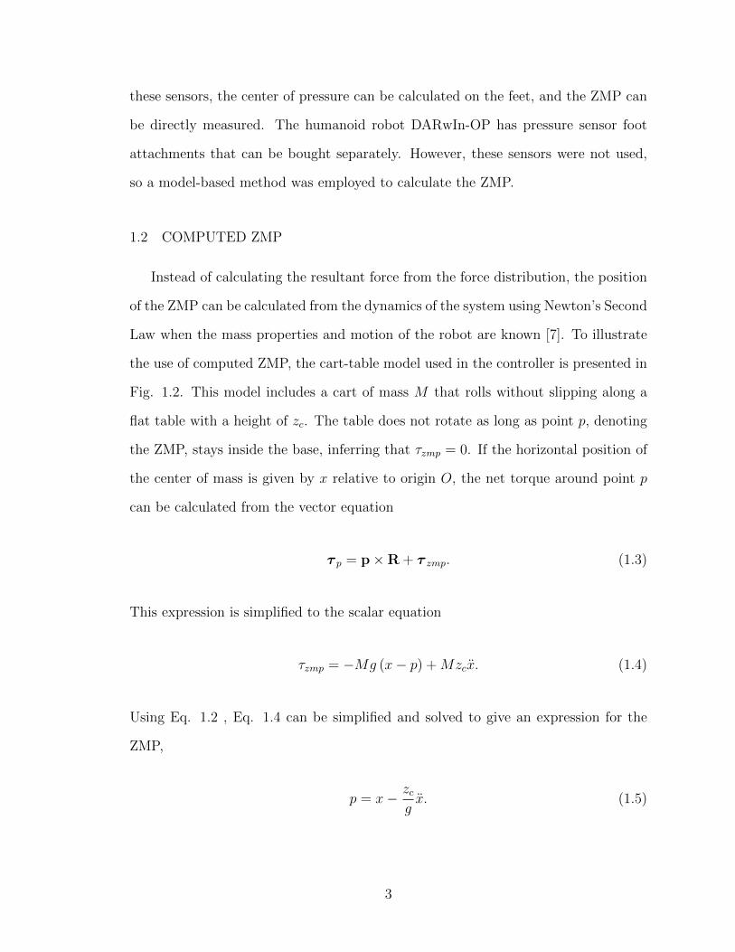
the use of computed ZMP, the cart-table model used in the controller is presented in

Fig. 1.2. This model includes a cart of mass M that rolls without slipping along a

flat table with a height of zc. The table does not rotate as long as point p, denoting

the ZMP, stays inside the base, inferring that τzmp = 0. If the horizontal position of

the center of mass is given by x relative to origin O, the net torque around point p

can be calculated from the vector equation

τ p = p×R + τ zmp. (1.3)

This expression is simplified to the scalar equation

τzmp = −Mg (x− p) +Mzcx. (1.4)

Using Eq. 1.2 , Eq. 1.4 can be simplified and solved to give an expression for the

ZMP,

p = x− zcgx. (1.5)

3

Figure 1.2. Cart-Table Model

Looking closer at Eq. 1.5 , two interesting observations emerge about the computed

ZMP from this definition.

1. The ZMP becomes the CoM when there is no acceleration.

2. The ZMP can be located outside the support polygon.

If the ZMP leaves the support polygon during the gait, the motion is determined to

be unstable because it can cause the robot to tip over about an edge of the support

polygon. This, however, does not necessarily mean that the robot will fall. For

example, if a bipedal robot has feet glued to the ground, the ZMP could be outside

the support polygon without the robot falling. The cohesive forces of the glue adds

an extra force to balance the torque around the ZMP so that the robot does not fall

until the glue fails. If falling, the robot can recover stable walking either through its

motion (compensating body movement) or increasing its support polygon (placing

the other foot on the ground).

The ZMP can also be calculated for the 3D case using Newton’s and Euler’s laws

for the change in linear and angular momentum. More general expressions, similar

to Eq. 1.5, were presented in [7] and summarized in Appendix A.2. This was used in

modeling the full 3D dynamics of DARwIn-OP to calculate the ZMP. However, this

4

3D model was never formally used in the controller, but was developed using Kane’s

method.

1.3 THE HUMAN GAIT AND A SIMPLIFIED MODEL

One of the goals of implementing this humanoid walking controller is to achieve

a walking gait that is more human-like. In order to achieve this, the human gait is

presented and then simplified to match the needs of the controller. During walking,

at least one foot remains in contact with the ground at all times. Each step consists

of two main phases, stance and swing, consisting of about 62% and 38% of the gait

cycle, respectively. Each of these phases can be subdivided into 8 more categories [4]:

initial contact, loading response, midstance, terminal stance, preswing, initial swing,

midswing, and terminal swing as shown in Fig. 1.3.

Figure 1.3. Human Gait Cycle [2]

When the leading foot touches the ground, initial contact begins, starting the

5

stance phase. Usually, this involves a simple heel strike to the ground. The main

implusive force from ground contact is experienced in the next phase, the loading

response. In this phase, the leading foot flattens, coming in full contact with the

ground. The leading foot then absorbs the contact force from the ground. After

this, the first single support phase, called midstance, begins when the trailing foot

leaves the ground and ends when the body weight is aligned over the front of the

current stance foot. During midstance, the body has a maximum potential energy

as the body’s center of gravity reaches its maximum height, rising over the stance

leg. The terminal stance phase begins as soon as the body’s weight shifts past the

current stance foot. Heel off occurs during this phase when the stance foot’s heel

leaves the ground. The final stance phase is preswing, in which the previous stance

foot prepares to lift off, but is still in contact with the ground. This is called toe off

as the previous stance foot’s toe leaves the ground and can no longer provide active

forward propulsion.

Now, the previous stance leg during single support becomes the swing foot for

the next three phases. Initial swing begins immediately after the swing foot leaves

the ground and lasts until maximum knee flexion, where midswing starts. During

midswing, the swing foot is brought past the stance foot, making sure that the foot

has enough ground clearance. The phase ends when the tibia is perpendicular to

the ground. The final phase, terminal swing, prepares the body for contact with the

ground and fully extends the knee. This completes one gait cycle [4].

In order to simplify the human gait cycle, the proposed controller is broken into

four distinct phases: right leg double support, right leg single support, left leg double

support, and left leg single support. Relating these to the aforementioned phases,

right leg double support tries to capture initial contact to midstance. Right leg single

support refers to the period of time during which the left leg is swinging through the

air, namely midstance and most of terminal stance. As soon as the left swing leg

6

touches the ground, left leg double support begins, which includes the last part of

terminal stance and preswing. The final part of the gait, left leg single support,

includes the entire swing phase from initial swing to terminal swing. The controller

develops schemes to handle these four phases throughout the walking gait cycle.

1.4 DARWIN-OP

For testing purposes, the controller was implemented on DARwIn-OP, a humanoid

developed at the Robotics and Mechanisms Laboratory (RoMeLa) at Virginia Tech

[3]. DARwIn-OP stands for dynamic anthropomorphic robot with intelligence - open

platform and is used for research and educational purposes. DARwIn-OP is a twenty-

degree-of-freedom mechanism with twenty MX-28 Dynamixel servo motors [1]. Each

of these servos has a 12 bit encoder with a resolution of 0.088◦, or values ranging from

0-4095 for 360◦ which are position controlled. Each of the legs contains six motors,

and each of the arms has three motors. The remaining two motors actuate the pitch

and yaw motions for the head.

Each of these twenty motors has a single axis of rotation, so coordinate systems

must be defined to describe the relative orientation between links. In Figure 1.4, the

axes of rotations for the joints are shown as red arrows. These directions were chosen

based on the positive rotational directions in hardware to ease the transformation

from model to implementation. A front view of DARwIn-OP is shown on the left, and

a side view is shown on the right. The global inertial coordinate frame is named the

N frame and is also shown in the diagram. When referring to a direction for walking

throughout this paper, the N frame is the coordinate system being referenced unless

otherwise stated. For example, walking forward is walking in the positive x direction.

Also, the N frame is located on the ground, directly between the feet in the y direction,

and in the middle of the feet in the x direction. The N frame location is denoted by

a � for each view in Fig. 1.4. The position of the N frame is important in defining

7

Figure 1.4. DARwIn-OP with Coordinate Systems

8

the reference trajectories for the CoM and the swing foot. This is the zero position

for DARwIn-OP so all of the joint coordinate systems are aligned with the N frame

except the shoulder roll is rotated 45◦ and the elbow is rotated -90◦. Arm swing was

not included in the controller, so this is not critical, but the zero position was used

for every joint that was uncontrolled. Therefore, all coordinate systems besides the

ones previously mentioned are aligned with the N frame and joint rotations can be

described in terms of roll (x-axis), pitch (y-axis), and yaw (z-axis) rotations. For

example, the right ankle has a joint with pitch in the negative y direction and a joint

with roll in the positive x direction.

Currently, DARwIn-OP has a walking controller programmed to locomote while

playing soccer. This walking controller creates a sinusoid for lateral body motion as

well as a step period to constantly be moving forward in time. Step parameters such

as stride length and stride width are used to achieve a desired goal location for the

swing foot. The swing foot also uses a sinusoid for ground clearance during the single

support phase. With this current controller, DARwIn-OP appears to take short,

choppy steps with a stride length usually less than DARwIn-OP’s foot length (104

mm). Going above this stride length usually leads to instability, or falling over. Using

the ZMP method, longer stride lengths are able to be obtained in a more predictable

manner that can be adjusted based on the step length, width, and period.

9

CHAPTER 2

METHODS

This chapter presents the scheme for the controller in order to accomplish a walk-

ing gait. A control law is developed using preview terms in order to track a reference

value. Trajectory generation for the main body’s CoM is accomplished through

a simple cart-table model, and the swing foot trajectory is determined through

parametrized equations.

2.1 CONTROLLER AND TRAJECTORY GENERATION SCHEME

In order to produce one gait cycle, the controller must account for the four different

phases: right leg double support, right leg single support, left leg double support, and

left leg single support. The double support and single support phases for each leg are

treated similarly due to the body symmetry in the xz plane. The two main parts of

the controller consist of tracking a CoM trajectory with the stance leg and following

a swing trajectory with the swing leg. From these two trajectories and additional

constraints, inverse kinematics can be used to calculate the desired angles. All of

these constraints are holonomic and enforced through geometry in all phases.

1. The stance leg and body behave like an inverted pendulum with varying length.

2. The body link is aligned with the N frame, or parallel to the ground.

3. The swing foot is also aligned with the N frame, or parallel to the ground.

10

Figure 2.1 shows a flow diagram for the individual components of the controller.

There are also knee flexion and body pitch controllers to directly control the stance

knee pitch and the body pitch, respectively. These controllers are crucial when tran-

sitioning between steps to maintain a cyclic pattern. Neglecting the body pitch

Figure 2.1. Control Scheme for the ZMP Walking Controller

and knee flexion controllers, the CoM trajectory and constraints 1 and 2 define all of

the stance angles for both the double support and single support phases. With these

angles, the swing foot trajectory, and constraint 3, the swing leg angles can now be

fully defined using inverse kinematics. This includes the assumption that ten of the

twelve leg joints were used in the controller, neglecting the two hip yaw joints. The

next sections define the details for each part of the controller.

11

2.1.1 DEFINING ANGLES

Before developing more details, there are two sets of angles that must be defined

to simplify the calculations for the inverse kinematics. One set is the local angles and

the other the global angles, both referencing the same axes of rotations for the joints

in Fig. 1.4. The local angles are defined by the stance and swing leg which switch as

the stance and swing legs change. A local angle is denoted simply by θ. However, the

global angles do not change and they identify a specific joint. These global angles are

simply denoted by θ′. Table 2.1 shows all the definitions for local and global angles.

For implementation, local angles are calculated and then transformed to global angles

depending on the phase.

TABLE 2.1: Local and Global Angle Definitions

θ Definition θ′ Definition

θ1 Stance Ankle Roll θ′1 Right Ankle Roll

θ2 Stance Ankle Pitch θ′2 Right Ankle Pitch

θ3 Stance Knee Pitch θ′3 Right Knee Pitch

θ4 Stance Hip Pitch θ′4 Right Hip Pitch

θ5 Stance Hip Roll θ′5 Right Hip Roll

θ6 Support Hip Roll θ′6 Left Hip Roll

θ7 Support Hip Pitch θ′7 Left Hip Pitch

θ8 Support Knee Pitch θ′8 Left Knee Pitch

θ9 Support Ankle Pitch θ′9 Left Ankle Roll

θ10 Support Ankle Roll θ′10 Left Ankle Pitch

2.2 CENTER OF MASS TRAJECTORY

Expanding the cart-table model to a 3D system, a CoM trajectory can be cal-

culated in the xy plane using the linearized system. The linearization of the 3D

12

cart-table model can be found in Appendix A.3, and the result shown in Fig. 2.2 is

a cart that can move along a flat table at a set height zc. Let the location of the

center of mass be c =

[x y z

]Tand the position of the ZMP be p =

[px py

]T.

The z-component of the position of the ZMP is zero because it is assumed to be on

the ground.

Figure 2.2. 3D Cart-Table Model

This system can be put into state-space form with the position of the ZMP in

the xy plane as the outputs. In order to control the ZMP, the jerk of the CoM was

chosen as the input because the acceleration terms must appear as a state to define

13

the position of the ZMP. With these inputs and outputs, the state space system is

d

dt

x

x

x

y

y

y

=

0 1 0 0 0 0

0 0 1 0 0 0

0 0 0 0 0 0

0 0 0 0 1 0

0 0 0 0 0 1

0 0 0 0 0 0

x

x

x

y

y

y

+

0 0

0 0

1 0

0 0

0 0

0 1

uxuy

(2.1)

pxpy

=

1 0 − zcg

0 0 0

0 0 0 1 0 − zcg

[x x x y y y

]T. (2.2)

The dynamics in the two dimensions are completely decoupled from each other and

identical, so that means the same control law can be developed for ux and uy. The

goal of this controller is to force the ZMP to follow an input reference value which

directly relates to the stance foot’s position. Without having some feedforward term

in the control law that accounts for future reference values, the actual ZMP does not

reach the reference value fast enough. In terms of walking, the robot is already on

the next step before its body can catch up.

Illustrating this point, consider a type 1 servo system described by Ogata [6] with

a control law

u = KIe−Kx, (2.3)

where ux = u for x =

[x x x

]Tand e = ex, and uy = u for x =

[y y y

]Tand

e = ey. The gain matrix K is a 1x3 matrix multiplying the states. The error in the

actual ZMP relative to the reference ZMP value is defined as

e = pref − p. (2.4)

14

Gains of KI = 40 and Kx =

[1 50 4

]Twere chosen by trial and error in simulation

and reference values prefx and prefy were generated. Section 3.1 goes into further detail

about how to generate the reference values. Simulation results using the cart-table

model and the controller in Eq. 2.3 are shown in Figure 2.3. In the simulation, the

ZMP value tries to track the reference value with the integral gain and state feedback,

but it cannot react fast enough to the changing reference. For the y direction, the

actual ZMP reaches the reference as soon as the reference changes. Therefore, this

is not a sufficient controller to force the ZMP to folllow a certain reference due to

this phase delay. The control law must have some terms that include future reference

values.

0 2 4 6 8−1

0

1

t

x

0 1 2 3 4 5 6

−0.05

0

0.05

t

y

ZMPCoMReference ZMP

ZMPCoMReference ZMP

Figure 2.3. Response of the Cart-Table Model Using No Preview Controller

15

2.2.1 PREVIEW CONTROLLER

A preview controller has a control law whose input is a function of future reference

values. Using these preview terms is similar to looking down the road while driving.

A reference value farther down the road, and not the car’s current position, is used

to steer the car. In considering a preview controller, the system in 2.1 must be

discretized because the preview terms need to use discrete reference values. Using a

sampling time of Ts, the system is discretized as

x (k + 1) = Ax (k) +Bu (k) , (2.5)

p (k) = Cx (k) , (2.6)

where

x (k) =

[x (kTs) x (kTs) x (kTs) y (kTs) y (kTs) y (kTs)

]T, (2.7)

u (k) =

[ux (kTs) uy (kTs)

]T, (2.8)

p (k) =

[px (kTs) py (kTs)

]T, (2.9)

A =

1 Ts T 2s /2 0 0 0

0 1 Ts 0 0 0

0 0 1 0 0 0

0 0 0 1 Ts T 2s /2

0 0 0 0 1 Ts

0 0 0 0 0 1

, B =

T 3s /6 0

T 2s /2 0

Ts 0

0 T 3s /6

0 T 2s /2

0 Ts

(2.10)

C =

1 0 zcg

1 0 zcg

. (2.11)

16

Assume that the actual ZMP needs to track the reference ZMP, pref . By preview-

ing NL time steps into the future, the discrete control law proposed by Katayama [5]

can be used.

u (k) = −GIe (k)−Gxx (x)−NL∑j=1

Gp (j) pref (k + j) , (2.12)

where e (k) = p (k) − pref (k). Now, the actual ZMP in the cart-table model can

sufficiently track the reference with this extra feedforward term. The simple block

diagram in Fig. 2.4 broadly illustrates the control signals for the preview control.

The gains GI ,Gx, and Gd are associated with the integral, state feedback, and preview

Figure 2.4. Block Diagram of Preview Controller

terms, respectively. These gains must be chosen to achieve proper tracking of the

ZMP without much phase delay. Katayama [5] describes a method for designing an

optimal preview controller for a discrete-time system, and the method is summarized

in Appendix B. Given a system of n states, m outputs, and r inputs, this method

17

tries to minimize the performance index

J =∞∑i=k

[eT (i)Qee (i) + ∆xT (i)Qx∆x (i) + ∆uT (i)R∆u (i)

](2.13)

at each time k, where Qe and R are m × m and r × r symmetric positive definite

matrices. The matrix Qx is an n× n symmetric non-negative definite matrix associ-

ated with the incremental state vector. Decoupling the system into separate x and y

components, the following values were chosen for the controller,

Qe = 0.1 , Qx =

0 0 0

0 0 0

0 0 0

, R = 1× 10−6, (2.14)

with a sampling time of Ts = 8 ms. Using the discrete-time system in Eqs. 2.7 to

2.11, the gains could be calculated using the linear quadratic regulator design for

discrete time systems described in Appendix B. Using the values in Eq. 2.14, the

gains were calculated to be GI = 257.7, Gx =

[10285.4 1683.3 1683.3

]T, and the

preview gains are shown in Fig. 2.5. The preview gains become negligible towards

the end of the previewing period. With these gains, the cart-table model can be

simulated, and Fig. 2.6 shows that the actual ZMP tracks the reference ZMP much

better without much phase delay.

In conclusion, the cart-table model is a simplified way to model the humanoid

as one large body mass accelerating in a plane at a constant height. The ZMP can

be controlled to follow a reference trajectory, and a CoM trajectory can be obtained

through simulation. The CoM trajectory is used in implementation with inverse

kinematics to calculate the stance leg angles.

18

0 0.5 1 1.5 20

100

200

300

400

t

Gp

Figure 2.5. Preview Gains Using the Optimal Controller Design

0 1 2 3 4−0.1

0

0.1

t

p y

0 1 2 3 4−0.2

0

0.2

0.4

t

p x

ZMPCoMReference ZMP

ZMPCoMReference ZMP

Figure 2.6. Response of the Cart-Table Model Using the Preview Controller

2.3 SWING FOOT TRAJECTORY

The stance leg uses the CoM trajectory and other constraints to define joint an-

gles, but the swing leg needs to establish a trajectory to define its angles. This

19

trajectory pswing tracks the location of the swing foot in the local foot frame F . The

F frame is aligned with the N frame, but it is located at the ankle joints of the

stance foot as shown in Fig. 2.7. The subscripts L and R denote the left and right

foot frames, respectively. The F frame switches between FL and FR depending on

the stance leg. Under the conditions that the humanoid is not tipping and the foot

is not slipping, the F frame is an inertial reference frame.

The swing foot trajectory pswing is defined relative to the current F frame. Con-

stantly updating the location of the F frame after each step requires the definition

of two more vectors. The stride vector for ith step, Si, locates the swing foot from

its position right before initial swing to right after terminal swing. The x and y com-

ponents of Si are the stride length and stride width, respectively. The foot reference

vector for the ith step, f refi , locates the swing foot before the initial swing phase.

Intermediate points along the swing foot trajectory are needed, so the following def-

inition is given.

pswing = si, (2.15)

where si is called the foot path vector which takes some path that starts at f refi and

ends at f refi + Si. A foot path function must be defined that calculates the value for

si at different times. The foot reference value is just a translational shift so the foot

path function has a similar shape to the plot in Fig. 2.8.

The swing leg trajectory needs to accomplish two distinct tasks:

1. Remain on the ground during the double support phase before swinging.

2. Establish a trajectory for the swing foot that reaches a specified stride length

Sx and width Sy within a certain single support period TSS.

With these tasks, the swing leg trajectory is split into the double support and single

support phases. The double support phase imposes that the swing foot remain on

20

Figure 2.7. Humanoid Feet with the F Frame and N Frame

the ground where it had landed, implying that pswing = f refi . The single support

phase is divided further into 3 different parts: initial swing, midswing, and terminal

swing. The time spent in initial swing and terminal swing is a percentage of the step

period, αTSS, and the rest of the time is spent in midswing. The final constraint on

the swing foot trajectory is that the swing foot must reach a certain height above

the ground called ground clearance cg. This prevents toe drag so that the toe does

not get too close to the ground. One possible swing foot trajectory is shown in Fig.

2.8 to illustrate the desired shape of the curve. The upper graph shows a side view,

while the lower graph shows a top view of the swing foot trajectory during the single

support phase given a stride vector S =

[0.104 0.01

]T.

2.3.1 INITIAL SWING

Initial swing occurs immediately after the double support phase ends and lasts for

αTSS seconds. The foot path function for the initial swing is marked by a parametriza-

tion to create an ellipse-type shape. Given a parametrized variable xt, the following

21

−0.1 −0.05 0 0.05 0.1−0.08

−0.07

−0.06

−0.05

x

y

−0.1 −0.05 0 0.05 0.10

0.02

0.04

0.06

0.08

Initial Swing Midswing Terminal Swing

t = 0

t = αTSS t = (1− α)TSS

t = TSS

x

z

Figure 2.8. Possible Swing Foot Trajectory, pswing

foot path function can be generated.

sx (xt) = −r cos (xt) + f refi,x (2.16)

sy (sx) = η(sx − f refi,x

)+ f refi,y (2.17)

sz (xt) = cg sin (xt), (2.18)

where 0 ≤ xt <π2

and

r = αSi,x. (2.19)

The r value is the length of one of the axes of the ellipse. This creates an ellipse

that is shifted by the foot reference value in the xz plane and linearly approaches the

stride width in the xy plane. The value for η can be calculated by a simple slope

formula,

η =Si,ySi,x

. (2.20)

22

Using time as the parametrized variable gives an easier result to implement in the xz

plane,

sx (t) = −r cos

(π

2αTSSt

)+ f refi,x (2.21)

sy (sx) = η(sx − f refi,x

)+ f refi,y (2.22)

sz (t) = cg sin

(π

2αTSSt

), (2.23)

where 0 ≤ t < αTSS. This defines the initial swing phase which lifts the foot off the

ground until it reaches the ground clearance cg.

2.3.2 MIDSWING

The next swing period, midswing, starts after initial swing and lasts until (1− α)TSS

seconds. During this phase, the foot stays at the constant ground clearance height

while moving forward in time. Laterally, the step width is accounted for in the same

manner through linear interpolation. To clearly show the relationship between the

time t and the current step length sx, a conversion constant is defined as b =Si,x

TSS.

For midswing, the foot path function is defined as

sx (t) = bt+ f refi,x (2.24)

sy (sx) = η(sx − f refi,x

)+ f refi,y (2.25)

sz (t) = cg, (2.26)

where αTSS ≤ t < (1− α)TSS.

2.3.3 TERMINAL SWING

The final swing phase is terminal swing, which occurs after midswing and prepares

the foot for ground contact. This has a very similar shape to initial swing except

23

that the function starts with the foot near ground clearance and brings the foot to

the ground. Again, the desired curve shape in the xz plane is an ellipse. One key

difference is the starting point for the step length sx must be shifted by a constant

since the terminal swing starts at sx (0) = f refi,x + (1− α)Si,x. Starting with the same

parametrized variable xt, the foot path function for terminal swing is

sx (xt) = r sin (xt) + f refi,x + (1− α)Si,x (2.27)

sy (sx) = η(sx − f refi,x

)+ f refi,y (2.28)

sz (xt) = cg cos (xt), (2.29)

where 0 ≤ xt <π2

and r = α(Si,x − f refi,x

). At the end of the period xt = π

2, the foot

path function must return final values of

sx = Si,x + f refi,x (2.30)

sy = Si,y + f refi,y (2.31)

sz = 0. (2.32)

Looking back at the previous equations describing the foot path function during

terminal swing, these all give the appropriate final values. Again, converting to time

gives

sx (t) = r sin( π

2αT(t− φ)

)+ f refi,x + (1− α) bTSS (2.33)

sy (sx) = η(sx − f refi,x

)+ f refi,y (2.34)

sz (t) = cg cos( π

2αT(t− φ)

), (2.35)

where φ = (1− α)TSS and φ ≤ t < TSS. With the foot path functions from initial

swing, midswing, and terminal swing, the swing foot trajectory is now defined and can

24

be used to calculate the swing leg angles. For implementation, the inverse kinematics

must be developed to actually calculate these angles.

25

CHAPTER 3

IMPLEMENTATION

This chapter develops an easy method to generate reference values for f ref and

pref . From the previously calculated trajectories, equations for the inverse kinematics

of the humanoid are used to calculate the joint angles. Constraints are used to define

all of the angles, and the body pitch and knee controllers are presented. Lastly, an

overview of the program used to implement the walking controller is explained.

3.1 REFERENCE GENERATION

To generate the two trajectories in the previous section, there were two references

that needed to be known. The foot reference f ref and the ZMP reference pref are

similar, but have subtle differences to provide more flexibility with the controller.

First, the foot reference defines the locations of the ankle joints and the F frame.

The support polygon can be determined from the foot reference. The ZMP reference

is just the desired location of the ZMP. The ZMP reference does not determine the

support polygon other than that the ZMP reference should be generated with the

understanding that the ZMP needs to be inside the support polygon.

Define a set of m steps S = [S0, S1, . . . , Sm−1, Sm], where S0 is an initialization

period, S1 is the first step, and Sm is the last step. S0 is a double support phase

that shifts the body mass toward the first stance foot, chosen to be the left foot, and

S0 =

[0 0 0

]T. Also, a ZMP reference offset δ is going to be added to the ZMP

reference equation in order to be able to shift the ZMP reference towards the outer

side of the foot or inside the foot. Adding this offset to the ZMP reference requires

26

knowledge of the stance foot, so a function that takes a step as an input and returns

a -1 or 1 based on the stance foot must be defined. For the ith step, this stance foot

function is

stance (Si) =

−1, if stance == RIGHT

1, if stance == LEFT.(3.1)

Figure 3.1 shows a visual of the reference vectors to more clearly formulate a

mathematical method to update these reference values. Looking at Fig. 3.1 and

using simple vector addition, the following update formulas can be used to define the

reference values after the initialization period.

f refi = −(f refi−1 + Srefi−1

)(3.2)

prefi = prefi−1 − f refi (3.3)

if i > 1. Then, the initial values must be set for the references. These are f ref1 =[0 −sw 0

]Tand pref0 =

[0 −1

2sw 0

]T, where the stance width sw is 0.074 m. It

is important to note that these are not the reference values during the initialization

period and are only used to update the values. Including the reference values for the

initialization terms and adding the offset to the ZMP reference, the two reference

trajectories become

f ref =

f ref1 , i = 0

f refi , i > 0.(3.4)

pref =

0, i = 0

prefi + (stance (Si) δ) j, i > 0. (3.5)

These initial values have a logical basis to them. Because the initialization period

27

Figure 3.1. Vectors used to Identify the Location of the Foot and ZMP atEach Step

does not have a single support phase, the foot reference is the same as the foot

reference of the first step. In other words, the stance foot has not changed. For

the ZMP reference, the updating equation in Eq. 3.3 allows for an easy method to

alternate between the left and right stance leg, but the ZMP needs to start in the

middle of the two feet if the robot is standing up straight with both feet on the

ground. Since the N frame is defined as the middle of the two feet initially, the ZMP

reference is the origin during the initialization period.

With only a set of steps and a predefined initialization period, foot and ZMP

reference values can be calculated from Eqs. 3.4 and 3.5. These reference values are

used with the formulations in the previous sections to calculate a CoM trajectory

and swing foot trajectory. With these trajectories, the inverse kinematics can be

developed in the local foot frame F to determine the angles.

28

3.2 INVERSE KINEMATICS

The following section develops angles for the local angle set defined in Table 2.1.

The relative angle of rotation is defined as the angle of rotation from the outer link

to the inner link of a joint. For global angles, the initial link is the body, but for the

local angles, the initial link is either foot depending on the stance leg. This means

that local swing angles are equivalent to their global angle counterparts, but local

stance angles are the negatives of their global angle counterparts. Global angles are

only used in implementing the software, and only local angles are discussed in future

sections.

The following assumptions are made while trying to track the CoM trajectory

and the swing leg trajectory.

1. All of the mass is located in the body along the stance hip pitch axis with

M = 2.93 kg.

2. The robot is symmetrical around the xz plane of the N frame.

3. The stance leg and body mass act like an inverted pendulum that can vary in

length.

These assumptions are used throughout the inverse kinematics formulation to simplify

some of calculations and the dimensions shown in Fig. 3.2. Another vector phip is

defined to locate the swing hip relative to the F frame. With these assumptions, the

leg lengths are the same, with a = 0.093 m, and l = 0.037 m, which is half of the

stance width. These dimensions are used frequently to locate the CoM and the swing

foot trajectories.

3.2.1 STANCE LEG

The strategy for the stance leg is to use the CoM trajectory to determine the

two ankle joint angles, the knee to determine the height of the body, and the two

29

Figure 3.2. Local Coordinate Systems for DARwIn-OP

hip joint angles to orient the body. First, the assumption about the behavior of the

stance leg and body as an inverted pendulum must be fully developed. The knee

angle determines the height of the inverted pendulum through the law of cosines.

Looking at the stance leg in Fig. 3.3, the bent knee forms a triangle with a height hp

being the height of the pendulum. This can be calculated using the law of cosines,

hp =√

2a2 (1− cos (π − θ3)). (3.6)

The angle constraints to maintain this inverted pendulum requires that

θ2 =1

2θ3 + more terms (3.7)

θ4 =1

2θ3 + more terms. (3.8)

Without more terms, the body would bend down, adjusting the height of the pendu-

lum based on the knee bend. More terms are included in θ2 to track the CoM, while

more terms are included in θ4 to orient the body using the body pitch controller.

30

Figure 3.3. Stance Leg Pitch Angles Forming the Height of the Pendulum

With this pendulum height, inverse kinematics for a 3D pendulum with a roll then

pitch joint at the base can be used to calculate the angles. However, the location of

the body mass must be identified relative to the F frame, and currently, the CoM

trajectory is relative to the N frame. This transformation is simply a translation

because the two coordinate systems are aligned. This translation f is the location of

the F frame relative to the N frame. For the ith step Si, this vector can be calculated

(see Fig. 3.1),

fi = pref0 −i∑

j=1

f refj . (3.9)

where pref0 =

[0 −1

2sw 0

]T. Now, the local CoM trajectory cN/F can be calculated

from the CoM trajectory c,

cN/F = c− f . (3.10)

Figure 3.4 shows the location of the foot, CoM trajectory, and local CoM trajectory

for the given gait of S0 =

[0 0 0

]T, S1 =

[12fl 0 0

]T, and S2 = S3 = S4 = S5 =

31

S6 = S7 =

[fl 0 0

]Twith an initialization period of T0 = 0.8 seconds and step

periods of T = 0.536 seconds. The local CoM cN/F has a very repeatable pattern,

but is discontinuous in time when the reference F frame changes. Returning to

0 50

0.2

0.4

f x

0 5−0.05

0

0.05

f y

0 50

0.2

0.4

c x

0 5−0.1

0

0.1

c y

0 5−0.05

0

0.05

t

c N/F,x

0 5−0.05

0

0.05

t

c N/F,y

Figure 3.4. Graphs for the f , c, and cN/F as Functions of Time for aPossible Gait

Fig. 3.3, the inverse kinematics for the 3D pendulum are slightly different based on

a left foot or right foot stance leg, so these are treated separately. If F = FR, the

location of the center of the mass relative to the F frame is

cN/F = CN 2(lj + hpk

), (3.11)

32

with the rotation matrices

CN 1 =

1 0 0

0 cθ1 −sθ10 sθ1 cθ1

, C1 2 =

cθ2p 0 sθ2p

0 1 0

−sθ2p 0 cθ2p

(3.12)

and CN 2 = CN 1 C1 2. The subscript p denotes an angle that is not the entire stance

ankle angle, but only the angle from the inverse kinematics of the 3D pendulum.

Separating these equations into their components yields

cN/F ,x = −hpsθ2p (3.13)

cN/F ,y = lcθ1 − hpcθ2psθ1 (3.14)

cN/F ,z = lsθ1 + hpcθ2pcθ1 . (3.15)

Solving 3.13 for θ2p gives

θ2p = sin−1(−cN/F ,x

hp

). (3.16)

From 3.14 and 3.15, θ1 can be calculated as

θ1 = sin−1

(lcN/F ,z − cN/F ,yhpcθ2p

l2 + h2pc2θ2p

)where (3.17)

cN/F ,z =√h2p + l2 − c2N/F ,x − c2N/F ,y. (3.18)

Equation 3.18 is derived from equating the lengths of the pendulum calculated using

the center of mass coordinates cN/F and the link lengths hp and l. When F = FL

33

and l < 0, these angles are

θ2p = sin−1(cN/F ,xhp

)(3.19)

θ1 = sin−1

(lcN/F ,z − cN/F ,yhpcθ2p

l2 + h2pc2θ2p

). (3.20)

A more complete derivation for these angles can be found in Appendix C. The only

difference between the left and right stance legs is in θ2p because the axis of rotation

of the ankle pitch is reversed for the left stance leg. Combining this result with Eq.

3.7 gives the stance ankle pitch angle

θ2 =1

2θ3 + θ2p . (3.21)

3.2.1.1 PARALLEL BODY CONSTRAINT

The only stance leg angles that need to be calculated in order to stand the body

upright are the stance hip roll and stance hip pitch. This relationship can be calcu-

lated geometrically through interior angles of the triangle formed by the knee bend.

The total roll rotation and total pitch rotation must be zero. Looking at Fig. 3.3

and accounting for the direction of rotation in Fig. 3.2, the relationship to keep the

body parallel to the ground for the pitch direction is

π

2= −θ4 +

π

2− θ3 + θ2, (3.22)

θ4 = θ2 − θ3. (3.23)

The constraint for the body roll is straightforward,

θ5 = θ1, (3.24)

34

although this does add error for the ankle joints that are attempting to track the

CoM because the stance leg is no longer perpendicular to the body, causing Eq. 3.11

to be slightly incorrect. This error is neglected due to the fact that the stance hip

and ankle joints should have very small rotations, and therefore, this error is very

small. The extra rotation for the stance hip pitch does not add any error to this

model because of the assumption that the CoM lies along the axis of rotation of the

stance hip pitch. Now, all the stance leg joint angles have been defined and can track

a CoM trajectory.

3.2.2 SWING LEG

The swing leg joint angles have a similar strategy. The inward joints angles for

the swing hip roll (θ6), swing hip pitch (θ7), and the swing knee pitch (θ8) are used

to track the swing foot trajectory pswing, while the two ankle joint angles attempt

to keep the foot parallel with the ground. Again, the formulations must be treated

differently for a left swing leg compared to a right swing leg, but for the concepts are

the same.

The first part in calculating the vector from F to the swing hip phip is exactly

the same for each swing leg under the assumption that l < 0 when F = FL. Using

forward kinematics, the vector loop equation is

CN 2

0

0

a

+ CN 3

0

0

a

+ CN 5

0

2l

0

+ CN 7

0

0

−a

+ CN 8

0

0

−a

= pN swing. (3.25)

35

Converting Eq. 3.25 to the stance hip roll frame (frame 5), the equation becomes

C5 2

0

0

a

+ C5 3

0

0

a

+

0

2l

0

+ C5 7

0

0

−a

+ C5 8

0

0

−a

= p5 swing, (3.26)

with the terms in parentheses equal to p5 hip. Substituting this value into Eq. 3.26

and rerranging gives

C5 7

0

0

−a

+ C5 8

0

0

−a

= p5 swing − p5 hip = ∆p5 . (3.27)

This is where the analysis must split into two different formulations depending on the

stance leg because the rotation matrices are not the same in Eq. 3.27. For notational

clarity, assume that ∆p = ∆p5 . If F = FR, the angles for the swing hip and knee

are

θ6 = ATAN2(−∆p2y,−∆p2z

)(3.28)

θ8 = −cos−1(

∆p2x + ∆p2y + ∆p2z − 2a2

2a2

)(3.29)

θ7 = ATAN2

(∆p2x (1 + cθ8) cθ6 + ∆p2zsθ8

2acθ6 (1 + cθ8),∆p2xsθ8cθ6 −∆p2z (1 + cθ8)

2acθ6 (1 + cθ8)

). (3.30)

A more complete derivation for these angles can be found in Appendix C. When

F = FL, ∆p must be slightly adjusted by changing ∆px,FL= −∆px,FR

. The swing

angles become very similar to those for the right leg as the swing leg except for a

36

sign change in the hip roll joint angle,

θ6 = ATAN2(−∆p2y,−∆p2z

)(3.31)

θ8 = cos−1(

∆p2x + ∆p2y + ∆p2z − 2a2

2a2

)(3.32)

θ7 = ATAN2

(∆p2x (1 + cθ8) cθ6 + ∆p2zsθ8

2acθ6 (1 + cθ8),∆p2xsθ8cθ6 −∆p2z (1 + cθ8)

2acθ6 (1 + cθ8)

). (3.33)

3.2.2.1 PARALLEL FOOT CONSTRAINT

The parallel foot constraint is similar to the parallel body constraint, except it is

not intuitive to establish the relationship geometrically. With the foot parallel to the

ground at all times, the humanoid can land flat during terminal swing and smoothly

transition into double support phase. With the foot being flat on the ground, the end

of the double support phase causes problems for the swing knee. In order to keep the

foot flat on the ground, the swing knee has to extend, and with large stride lengths,

the knee may not be able to satisfy this constraint.

The method for calculating the swing ankle angles uses rotational matrices,

CN 10 = I3×3 (3.34)

C8 N CN 10 = C8 N (3.35)

C8 10 = C8 N , (3.36)

because C8 N can be calculated from the previous joint angles. Therefore, looking at

C8 10 for F = FR,

C8 10 =

cθ9 0 −sθ9

sθ10sθ9 cθ10 cθ9sθ10

cθ10sθ9 −sθ10 cθ9cθ10

, (3.37)

37

the swing ankle joint angles are

θ9 = ATAN2 (−m13,m11) (3.38)

θ10 = ATAN2 (−m32,m22) , (3.39)

where mij represents the element in the ith row and jth column of the matrix C8 N .

When F = FL, these swing ankle joint angles become

θ9 = ATAN2 (m13,m11) (3.40)

θ10 = ATAN2 (−m32,m22) . (3.41)

Finally, all of the trajectories and constraints for this controller have been satisfied.

The stance leg behaves like an inverted pendulum trying to track the CoM trajectory.

The stance leg also has the constraint that the body must be parallel to the ground,

defining the stance hip joint angles. The swing leg defines the swing hip and knee

joint angles by tracking the swing foot trajectory, and the constraint of a flat foot

defines the swing ankle joint angles.

3.3 CONTROLLER ADDITIONS

The controller is not complete yet though. There are a few additional parts

to add in order to easily adjust the control and provide a stable walking pattern.

Most of these were added after experimentation with the idea of compensating for

the simplified model. The first of these controllers is a body pitch controller, which

allows the main body to maintain a desired goal pitch instead of being parallel to the

ground. All that is needed to achieve this desired body pitch is an additional term

38

in Eq. 3.23 for the desired body pitch,

θ4 = θ2 − θ3 + θbp, (3.42)

where θbp is the pitch of the main body. Since the body pitch may be different when

the stance leg changes, a controller is necessary to force the body pitch to remain

at the desired body pitch angle θbpd . This controller uses a proportional control law

which acts like a servo system,

θbp = θbp +Kbp (θbpd − θbp) . (3.43)

This forces the body pitch angle to approach the desired value because the term

with the proportional gain on the right-hand side of the equation will be zero near

the desired value. The value for Kbp used during simulation and testing was 0.05.

During implementation, this body pitch angle must be recalculated by rearranging

Eq. 3.42 for θbp whenever the stance leg changes. This body controller compensates

for forward and backward tipping.

The next controller addition was a knee flexion controller. This knee flexion

controller is important to a stable, smooth, and repeatable walking gait. After the

stance leg changes, there is no guarantee that the knee flexion is still at the same

constant angle, and in fact, it is not going to be unless the stride length happens

to be exactly the proper length. Therefore, a similar proportional controller can be

used to control the knee flexion to a desired value,

θ3 = θ3 +Kkf (θkf − θ3) , (3.44)

where θkf is the desired knee flexion. The value for Kkf used during simulation and

testing was 0.10. The graphs in Fig. 3.5 clearly show the effect of the knee flexion

39

0 5

0.7

0.8

0.9

1

1.1

1.2

1.3

1.4

t

θ′ 3

0 5−1.3

−1.2

−1.1

−1

−0.9

−0.8

−0.7

−0.6

t

θ′ 8

0 5

0.7

0.8

0.9

1

1.1

1.2

1.3

t

θ′ 3

0 5−1.3

−1.2

−1.1

−1

−0.9

−0.8

−0.7

−0.6

t

θ′ 8

Figure 3.5. Global Knee Angles without (left) and with (right) KneeFlexion Controller

controller. Without the knee flexion controller, the knee angles stay constant during

double support phase, and the knee bends more and more with each double support

phase. The knee flexion controller forces the knee flexion to maintain a cyclic and

sustainable pattern during walking.

The final addition to the walking controller seems unjustified and random at first

glance. This part of the controller adds a constant value to offset the CoM trajectory

in the y direction so that

c′ = c + ν j, (3.45)

where c′ is the adjusted CoM trajectory with this offset, which is used as the actual

CoM trajectory. The reason this was added to the controller is to compensate for the

error in the assumption of symmetry in the xz plane. According to the multibody

mass model, this is not true, and the CoM is in fact shifted toward the right foot

by about 3 mm. This approach had a noticeable effect in experiments when setting

ν = 0.005, or 5 mm. When the actual CoM is toward the right leg, ν > 0 to properly

40

shift the CoM. All of these additional controllers try to compensate for errors in the

model and provide easy methods for controlling crucial angles such as the body pitch

and knee flexion.

3.4 PROGRAMMING SYNOPSIS

A brief summary of the program algorithm is provided for a full understanding

and example of the implementation of the controller. The algorithm is divided into

3 different sections: a ZMP walking controller, a step manager, and the cart-table

dynamics. Each of these divisions includes important tasks that were previously

described. The algorithm for the controller is shown in the flow chart shown in Fig.

3.6.

The ZMP walking controller’s main task is to complete the current step move-

ment. The main data associated with a step are its stride length and width, the CoM

trajectory, the swing foot trajectory, and its step period (double support and single

support period). These steps are held in a data structure that acts like a queue. The

ZMP walking controller executes the current step by computing the angles through

inverse kinematics until the step has finished. When the step is complete, the ZMP

walking controller requests the next step from the step manager.

The step manager facilitates the transfer of data between the ZMP walking con-

troller and the cart-table dynamics. This is where all the step data is stored and

where the queue of steps is implemented. It is important to note that DARwIn-OP

could not allocate more than 500 bytes of data dynamically, which means that only

data for 6 steps could be stored at once, with a maximum step period of T = 800ms.

This is the maximum because the data is stored as one big chunk at the beginning

to avoid dynamically storing data. The reason to avoid dynamic memory allocation

is for one time step of ∆t = 8ms, just storing the CoM trajectory and swing foot

trajectory is 48 bytes. Therefore, the maximum chunk of dynamic memory that can

41

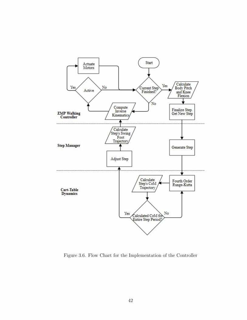
Figure 3.6. Flow Chart for the Implementation of the Controller

42

be allocated at once (500 bytes) can only store 80ms of CoM and swing foot positions.

After the current step is complete, the step manager creates a new step through

a set of step parameters, such as stride length or step period. This step gets added

onto the end of the queue, but the CoM trajectory cannot be calculated for this step

because there are no steps ahead of it to preview. The queue has three pointers that

point to a set of data for one step, pictured as a row in Fig. 3.7. The first pointer,

called ‘current’, stores a pointer to the current step data. The second pointer, ‘cal-

culated’, stores a pointer to the next step that needs the CoM trajectory calculated.

The final pointer,‘last’, points to the last step in the queue. These are all incremented

at the appropriate times to achieve the queue data structure. The cart-table

Figure 3.7. Representation for the Queue of Steps in the Step Manager

dynamics division of the controller calculates the CoM trajectory given the next step

to be calculated. This uses fourth order Runge-Kutta as a numerical integrator and

previews into the next steps for 1.6 seconds. After this is calculated, the step period

must be adjusted by the step manager to determine how to divide the step period

into a double support phase period TDS and a single support phase period TSS. The

idea is that when the ZMP enters the support foot polygon, the humanoid can leave

43

the double support phase, and when the ZMP leaves the support foot polygon, the

double support phase begins and single support phase ends. This way, the difference

between the locations of the F frame and the ZMP can be used to determine where

the ZMP is relative to the support foot polygon,

d = |f − p|. (3.46)

The location of the inner front corner of the foot is 0.022 m in the y direction and

0.052 m in the x direction. Starting at the beginning of the step in double support,

the end of the double support phase is found when the ZMP crosses into the support

foot’s polygon. Mathematically, this relationship is

dx < 0.052 && dy < 0.022 (3.47)

due to the absolute value in Eq. 3.46 and the assumption that the ZMP always

enters the support foot’s polygon through the interior side or bottom edge and leaves

through the interior side or front edge. The end of single support can then be found

by starting at the end of the step and backstepping until Eq. 3.47 holds. Finally, all

the tools have been presented to implement this walking controller in DARwIn-OP.

44

CHAPTER 4

RESULTS AND DISCUSSION

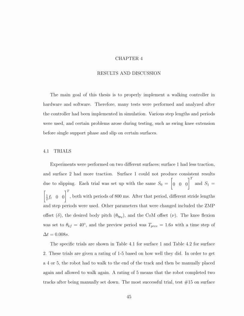
The main goal of this thesis is to properly implement a walking controller in

hardware and software. Therefore, many tests were performed and analyzed after

the controller had been implemented in simulation. Various step lengths and periods

were used, and certain problems arose during testing, such as swing knee extension

before single support phase and slip on certain surfaces.

4.1 TRIALS

Experiments were performed on two different surfaces; surface 1 had less traction,

and surface 2 had more traction. Surface 1 could not produce consistent results

due to slipping. Each trial was set up with the same S0 =

[0 0 0

]Tand S1 =[

12fl 0 0

]T, both with periods of 800 ms. After that period, different stride lengths

and step periods were used. Other parameters that were changed included the ZMP

offset (δ), the desired body pitch (θbpd), and the CoM offset (ν). The knee flexion

was set to θkf = 40◦, and the preview period was Tprev = 1.6s with a time step of

∆t = 0.008s.

The specific trials are shown in Table 4.1 for surface 1 and Table 4.2 for surface

2. These trials are given a rating of 1-5 based on how well they did. In order to get

a 4 or 5, the robot had to walk to the end of the track and then be manually placed

again and allowed to walk again. A rating of 5 means that the robot completed two

tracks after being manually set down. The most successful trial, test #15 on surface

45

2, had a step period of T = 0.536 seconds with a step length of the foot length fl.

TABLE 4.1: Tests on Surface 1

Test # S [m] T [s] δ [m] θbpd [◦] ν [m] Rating

0 fl 0.8 0.011 - - 1

1 fl 0.8 0.011 5 - 3

2 fl 0.8 0.011 10 - 2

3 fl 0.6 0.011 10 - 4

4 fl 0.8 0.011 10 - 2

TABLE 4.2: Tests on Surface 2

Test # S [m] T [s] δ [m] θbpd [◦] ν [m] Rating

0 fl 0.8 0.011 15 - 2

1 fl 0.8 0.011 15 - 4

2 fl 0.8 0.011 15 - 4

3 fl 0.6 0.015 15 - 2

4 fl 0.6 0.020 15 - 2

5 fl 0.6 0.025 15 - 1

6 fl 0.536 0.011 10 - 2

7 fl 0.536 0.02 10 0.003 2

8 fl 0.536 0.011 10 0.005 3

9 fl 0.536 0.011 10 0.005 5

10 fl 0.536 0.011 10 0.005 5

11 54fl 0.536 0.011 10 0.005 5

12 32fl 0.536 0.011 10 0.005 2

13 fl 0.8 0.011 15 0.005 2

14 fl 0.536 0.011 10 0.005 4

15 fl 0.536 0.011 10 0.005 5

46

4.2 DISCUSSION

Most of the tests were successful in starting off stable after the initialization period

when the body pitch controller as well as the CoM offset were added to the controller.

Some of the main problems causing instability included slipping of the support foot

and swing foot interference with the stance foot. Slipping occurred frequently during

the double support phase before initial swing, while the knee has a quick extension

period. This quick extension is caused by the constraint to keep the stance foot on

the ground as the body moves forward quickly to shift the ZMP into the stance foot’s

support polygon. This knee extension problem was exaggerated with larger stride

lengths in test #13 for surface 2. This problem could be alleviated by implementing

toe off to allow the heel of the stance foot to lift off the ground during double support

phase.

Interference of the swing foot and the stance foot occurred occassionally. The

result was the swing foot never reached its proper goal and did not land completely

with a flat foot. This interference was not caused by an improper swing foot trajec-

tory. In fact, the robot’s own weight was causing the swing leg to move closer to the

stance foot and slightly hit the stance foot. This was tested by lifting the robot off

the ground to check for interference, and no interference was observed. This problem

can be alleviated with toe off as well because the higher CoM from less knee flexion

can cause less ankle roll.

These tests, especially the first few, demonstrated the need for the body pitch

controller as well as the CoM offset. In test # 0 on surface 1, the robot kept falling

backwards after the first step. By supporting its back, the robot was able to walk

and was laterally stable. The body pitch controller stabilized this backwards falling

motion by pitching the body forward. The need for the CoM offset became evident

after a few trials with the robot. These trials showed that after one or two gait cycles,

the robot was repeatedly falling over the inner part of the left stance foot. By shifting

47

the modeled CoM trajectory to the left (+y direction) due to the fact that the actual

CoM was shifted toward the right in the model, the walking gait no longer fell over

the inner part of the left stance foot.

The knee flexion controller was critical to maintaining the assumptions made and

a cyclic walking pattern. If the stance knee joint angle kept decreasing throughout

time, the robot got closer and closer to the ground, which is not a realistic gait.

The knee flexion controller and body pitch controller isolated key parameters to ad-

just during different trials. When different stride lengths or step periods were used,

adjusting the body pitch stabilized the walking gait in many trials. A body roll

controller should be considered in order to control the full orientation of the body.

4.3 FUTURE WORK

Possible future work includes improving some of the missing parts in modeling

human walking. More phases of the human walking gait could be modeled instead of

the four currently implemented. The most important improvment would be to add

toe off to the controller during the double support phase. This toe off would allow

the knee flexion to decrease and simulate human walking more closely. Toe off could

also be used to push the swing foot forward to begin the initial swing phase.

Another addition to the controller is a better estimate of the error in the ZMP

from the cart to the real system. This can be accomplished by using the multibody

3D model to calculate the ZMP. An error can be found between the 3D model and

the cart-table model. This error could be used to adjust the CoM trajectory in some

manner to create a better estimate of the actual ZMP.

DARwIn-OP has an accelerometer and gyroscope, which has the ability to provide

some sensor feedback. This sensor feedback can be added to the walking controller

in a variety of different ways. For example, the inputs from the gyroscope and

accelerometer could be used to approximate the ZMP and then adjust the CoM

48

trajectory based on the values that are being sensed.

4.4 CONCLUSION

This thesis establishes a simple and elegant walking controller that achieves a

stable and adjustable walking gait in DARwIn-OP. Although simplified, using the

cart-table model produced a steady and sufficient CoM trajectory to track using

the stance leg. This walking controller produced a steady gait for a range of step

periods, 0.536s < T < 0.8s, and step lengths 0.104m < Sx < 0.130m. The body

pitch and knee flexion controllers greatly assisted in stabilizing the gait, and the

stride length can be increased by adding toe off to the controller. Further work must

be accomplished to improve the controller in order to have feedback while walking

and improve the walking gait pattern itself to better model a human gait.

49

APPENDIX A

ZERO-MOMENT POINT

A.1 TORQUE ABOUT ZMP

The derivation for the torque around the ZMP is given in chapter 16 of the

Springer Handbook for Robotics [7]. Recall that

p =

∑Ni=1 pifiz∑Ni=1 fiz

. (A.1)

Given a set of contacting points pi for i = 1, . . . , N with force vectors fi fixed in the

ground with a line of action through pi, the net torque about the ZMP is

τ =N∑i=1

(pi − p)× fi. (A.2)

Writing this vector equation in its different components yields

τx =N∑i=1

(piy − py) fiz −N∑i=1

(piz − pz) fiy (A.3)

τy =N∑i=1

(piz − pz) fix −N∑i=1

(pix − px) fiz (A.4)

τz =N∑i=1

(pix − px) fiy −N∑i=1

(piy − py) fix. (A.5)

50

Mathematically, a horizontal floor means that piz = pz because the ZMP must remain

on the floor. Substituting Eq. A.1 into Eqs. A.3 and A.4 simplifies the equations to

τx = τy = 0 (A.6)

at the Zero-Moment Point. This is how the Zero-Moment Point gets its name.

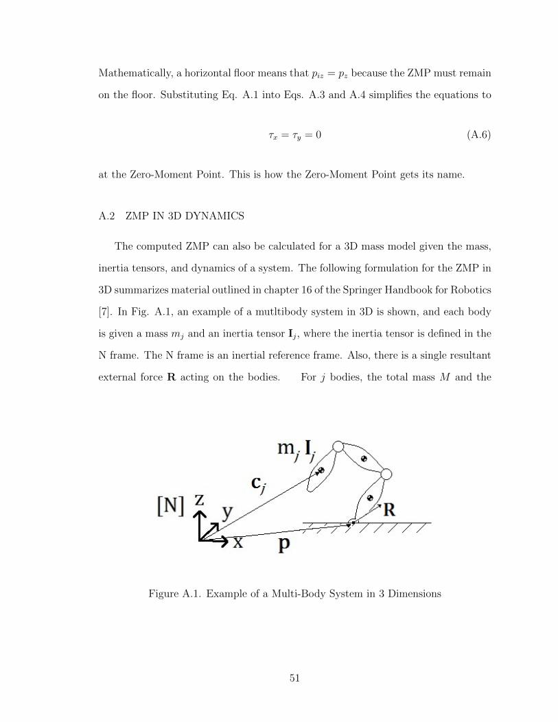
A.2 ZMP IN 3D DYNAMICS

The computed ZMP can also be calculated for a 3D mass model given the mass,

inertia tensors, and dynamics of a system. The following formulation for the ZMP in

3D summarizes material outlined in chapter 16 of the Springer Handbook for Robotics

[7]. In Fig. A.1, an example of a mutltibody system in 3D is shown, and each body

is given a mass mj and an inertia tensor Ij, where the inertia tensor is defined in the

N frame. The N frame is an inertial reference frame. Also, there is a single resultant

external force R acting on the bodies. For j bodies, the total mass M and the

Figure A.1. Example of a Multi-Body System in 3 Dimensions

51

center of mass c of all the bodies are

M =N∑j=1

mj (A.7)

c =1

M

N∑j=1

mjcj. (A.8)

The total linear momentum P and total angular momentum L with respect to the N

frame can be defined from the time derivatives of the centers of mass of the bodies

as

P =N∑j=1

mj cj (A.9)

L =N∑j=1

[cj × (mj cj) + Ijωj] , (A.10)

where ωj is the angular velocity of the jth body. Calculating the external torque

about the origin gives

τ = p×R + τ zmp, (A.11)

where τ zmp is the moment at p whose x and y components are zero according to

Eq. A.6. Defining g as the gravitational acceleration vector,

[0 0 −g

]T, and

substituting Newton’s and Euler’s laws,

R = P −Mg (A.12)

τ = L − c×Mg, (A.13)

52

into Eq. A.11 yields

τ zmp = L − c×Mg +(P −Mg

)× p. (A.14)

Dividing the vector equation into its individual components, the equations in the x

and y direction are

τzmp,x = Lx +Mgy + Pypz −(Pz +Mg

)py (A.15)

τzmp,y = Ly −Mgx− Pxpz +(Pz +Mg

)px. (A.16)

Using the definition of the ZMP in Eq. A.6 and solving for the ZMP position vector,

Eqs. A.15 and A.16 become

px =Mgx+ pzPx − Ly

mg + Pz(A.17)

py =Mgy + pzPy − Lx

mg + Pz. (A.18)

These equations can then be used to calculated the location of the ZMP with any

multibody 3D system.

A.3 3D LINEARIZED CART-TABLE MODEL

Given the 3D cart-table model in Fig. A.2, the cart on top of the table can move

along the top of the table in any direction without slipping. The cart always remains

in contact with the top of the table as well, and there is no friction force between the

base of the cart and the ground. The position of the cart is given by c =

[x y z

]T,

and the cart has a mass of M . Calculating the the linear momentum P and its

53

Figure A.2. 3D Cart-Table Model

time derivative gives,

P = M(xi + yj + zk

)(A.19)

P = M(xi + yj + zk

). (A.20)

Calculating the angular momentum L about the origin of the N frame and calculating

its time derivative yields

L = c×M c = M[(yz − zy) i + (zx− xz) j + (xy − yx) k

](A.21)

L = M[(yz − zy) i + (zx− xz) j + (xy − yx) k

]. (A.22)

Now substituting values into Eqs. A.17 and A.18 gives

px (x, z, x, z) =gx− zx+ xz

g + z(A.23)

py (y, z, y, z) =gy + yz − zy

g + z. (A.24)

54

Now, both of these equations must be linearized about the point x = y = 0, x = y =

z = 0, and z = zc. The linearized system takes the form of

pxpy = J

{x x x y y y z z z

}T, where (A.25)

J =

∂px∂x ∂px∂x

∂px∂x

∂px∂y

∂px∂y

∂px∂y

∂px∂z

∂px∂z

∂px∂z

∂py∂x

∂py∂x

∂py∂x

∂py∂y

∂py∂y

∂py∂y

∂py∂z

∂py∂z

∂py∂z

(A.26)

and J is the Jacobian matrix. Taking the partial derivatives with respect to each

variable for Eqs. A.23 and A.24 yields

∂px∂x

= 1 (A.27)

∂px∂z

= − x

g + z(A.28)

∂px∂x

= − z

g + z(A.29)

∂px∂z

=xz

(g + z)2(A.30)

∂py∂y

= 1 (A.31)

∂py∂z

= − y

g + z(A.32)

∂py∂y

= − z

g + z(A.33)

∂py∂z

=yz

(g + z)2. (A.34)

Substituting these into the Jacobian and evaluating at the linearization point gives

the linearized system

pxpy =

1 0 −zcg

0 0 0 0 0 0

0 0 0 1 0 −zcg

0 0 0

{x x x y y y z z z

}T.

(A.35)

55

Notice that the linearized system is no longer a function of z and its time deriva-

tives, so this state can be removed from the system. Essentially this removes the

translational joint on the table so that the cart cannot move up or down.

56

APPENDIX B

OPTIMAL CONTROL DESIGN FOR A PREVIEW CONTROLLER

This appendix provides a short description of how to implement the preview con-

troller described by Katayama [5]. Consider a time-invariant linear discrete system,

x (k + 1) = Ax (k) +Bu (k) + Ew (k) (B.1)

y (k) = Cx (k) , (B.2)

where x (k) is the n × 1 state vector, u (k) is the r × 1 control vector, y (k) is the

m × 1 output vector to be cotnrolled, and w (k) is the q × 1 inaccessible constant

disturbance. The incremental state vector is

∆x (i+ 1) = A∆x (i) +B∆u (i) , i = k, k + 1, . . . , (B.3)

removing the disturbance w (k) because it is a step function. The tracking error is

e (i+ 1) = e (i) + CA∆x (i) + CB∆u (i)−∆yd (i+ 1) , i = k, k + 1, . . . , (B.4)

where ∆yd (i+ 1) is the difference between the output from the next time step and

the current time step. With NL future demands yd (i) , i = k+1, . . . , k+NL available

at time k, the incremental demand can be placed in a pNL × 1 vector

xd (k) =

[∆yTd (k + 1) , . . . ,∆yTd (k +NL)

]T(B.5)

57

which satisfies

xd (i+ 1) = Adxd (i) i = k, k + 1, . . . , (B.6)

where

Ad =

0 Ip 0

0. . .

. . . Ip

0 0

. (B.7)

The incremental state vector, the tracking error, and the incremental demand vector

can create an augmented state vector,

x (i) =

[eT (i) ∆xT (i) xtd (i)

]T. (B.8)

Then, Eqs. B.3, B.4, and B.6 can be combined into

x (i+ 1) =

Ip CA −Ip 0 . . . 0

0 A 0 0 . . . 0

0 0 Ad

x (i) +

CB

B

0

∆u (i) , i = k, k + 1, . . .

(B.9)

Now, Qe, Qx, and R must be chosen, which are m×m, r× r, and n×n, respectively.

For example, the 1D cart-table system would have a Qe with dimensions 1× 1, a Qx

with dimensions 3 × 3, and an R with dimensions of 1 × 1. The ‘dlqr’ command in

MATLAB can be used with the augmented A and B matrices found in Eq. B.9 and

58

the Q and R matrices, where

Q =

Qe 0 0

0 Qx 0

0 0 0

. (B.10)

59

APPENDIX C

INVERSE KINEMATICS

In this section, the inverse kinematics for the CoM tracking and the swing foot

tracking are fully developed. First, the specific rotational matrices must be defined

for both the FL frame and FR frame. For the FR frame, the rotations based on local

angles are

CN 1 =

1 0 0

0 cθ1 −sθ10 sθ1 cθ1

C1 2 =

cθ2 0 −sθ20 1 0

sθ2 0 cθ2

C2 3 =

cθ3 0 sθ3

0 1 0

−sθ3 0 cθ3

C3 4 =

cθ4 0 sθ4

0 1 0

−sθ4 0 cθ4

C4 5 =

1 0 0

0 cθ5 sθ5

0 −sθ5 cθ5

C5 6 =

1 0 0

0 cθ6 sθ6

0 −sθ6 cθ6

C6 7 =

cθ7 0 −sθ70 1 0

sθ7 0 cθ7

C7 8 =

cθ8 0 −sθ80 1 0

sθ8 0 cθ8

C8 9 =

cθ9 0 sθ9

0 1 0

−sθ9 0 cθ9

C9 10 =

1 0 0

0 cθ10 −sθ100 sθ10 cθ10

.

For the FL frame, the stance leg and swing leg switch, so θ6 switches with θ5, θ7

switches with θ4, and so on. For notational simplicity, let cN/F = xi + yj + zk.

60

Calculating the forward kinematics for the CoM trajectory and referencing Fig 3.2,

cN/F = CN 2(lj + hpk

), (C.1)

and separating Eq. C.1 into separate components yields

x = −hpsθ2 (C.2)

y = lcθ1 − hpcθ2sθ1 (C.3)

z = lsθ1 + hpcθ2cθ1 . (C.4)

θ2 can be directly solved from Eq. C.2,

θ2 = sin−1(x

hp

). (C.5)

Solving Eq. C.4 for cθ1 ,

cθ1 =z − lsθ1hpcθ2

, (C.6)

and substituting the result into Eq. C.3

yhcθ2 = lz − l2sθ1 − h2pc2θ2sθ1 (C.7)

sθ1(l2 + h2pc

2θ2

)= zl − yhpcθ2 (C.8)

θ1 = sin−1(lz − yhpcθ2l2 + h2pcθ1

). (C.9)

However, z is not explicitly formulated in the CoM trajectory. Therefore, z must be

calculated by calculating the length of the pendulum with two different methods and

equating them. The first way uses the link lengths hp and l, and the second method

61

uses the distance formula for the center of mass, cN/F . This equation is

h2p + l2 = x2 + y2 + z2, (C.10)

and solving for z gives

z =√h2p + l2 − x2 − y2. (C.11)

Also note that when F = FR, l = 0.037, but when F = FL, l = -0.037.

Expanding the forward kinematics for the swing leg in Eq. 3.27 into individual

components yields

∆px = a (sθ7+θ8 + sθ7) (C.12)

∆py = −asθ6 (cθ7+θ8 + cθ7) (C.13)

∆pz = −acθ6 (cθ7+θ8 + cθ7) . (C.14)

By squaring and adding all three of these equations together, the result is

∆p2x + ∆p2y + ∆p2z = a2[(sθ7+θ8 + sθ7)

2 + (cθ7+θ8 + cθ7)2]

= 2a2 (sθ7+θ8sθ7 + cθ7+θ8cθ7 + 1)

= 2a2 (1 + cθ8) (C.15)

θ8 = −cos−1(

∆p2x + ∆p2y + ∆p2z − 2a2

2a2

). (C.16)

62

This negative sign is added to Eq. C.16 because θ8 > 0 is not within the joint limits

of the left knee pitch joint angle. Using Eqs. C.13 and C.14, θ6 can be determined.

sθ6 =−a∆py

cθ7+θ8 + cθ7(C.17)

cθ6 =−a∆pz

cθ7+θ8 + cθ7(C.18)

θ6 = ATAN2 (−∆py,−∆pz) . (C.19)

Solving for the knee pitch θ7 is more difficult. This requires Eq. C.12 to be solved

twice, once for sθ7 and once for cθ7 , after expanding the equation through trigono-

metric identities.

sθ7 =∆pzsθ8 + ∆pxcθ6 (1 + cθ8)

2acθ6 (1 + cθ8)(C.20)

cθ7 =∆pxsθ8cθ6 −∆pz (1 + cθ8)

2acθ6 (1 + cθ8)(C.21)

θ7 = ATAN2 (sθ7 , cθ7) . (C.22)

The forward kinematics can be calculated when F = FL, and the equations are very

similar to the previous forward kinematic equations,

∆px = −a (sθ7+θ8 + sθ7) (C.23)

∆py = −asθ6 (cθ7+θ8 + cθ7) (C.24)

∆pz = −acθ6 (cθ7+θ8 + cθ7) , (C.25)

except Eq. C.23 is multiplied by -1. If ∆px is multiplied by -1, the same Eqs. C.19,

C.22, and C.16, can be used to solve for θ6, θ7, and θ8, respectively when F = FL.

63

BIBLIOGRAPHY

1. Mx-28. Website, 2010. http://support.robotis.com/en/product/dynamixel/rx_series/mx-28.htm.

2. History of the study of locomotion. Website. http://www.

clinicalgaitanalysis.com/history/modern.html.

3. Darwin op: Open platform humanoid robot for research and education. Website,2011. http://www.romela.org/main/DARwIn_OP:_Open_Platform_Humanoid_

Robot_for_Research_and_Education.

4. E. Ayyappa. Normal human locomotion, part 1: Basic concepts and terminology.Journal of Prosthetics & Orthotics, 9(1):10–17, 1997.

5. T. Katayama. Design of an optimal controller for a discrete-time system subject topreviewable demand. International Journal of Control, Automation and Systems,41(3):677–699, 1985.

6. K. Ogata. Modern Control Engineering. Prentice Hall, Indianapolis, fifth edition,2010.

7. B. Siciliano and O. Khatib. Springer Handbook of Robotics. Springer, New York,illustrated edition, 2008.

8. M. Vukobratovic and J. Stepanenko. On the stability of anthropomorphic systems,mathematical biosciences. 15:1–37, 1972.

This document was prepared & typeset with pdfLATEX, and formatted withnddiss2ε classfile (v3.2013[2013/04/16]) provided by Sameer Vijay and updated

by Megan Patnott.

64